A Hidden Challenge of Link Prediction:
Which Pairs to Check?

Abstract

The traditional setup of link prediction in networks assumes that a test set of node pairs, which is usually balanced, is available over which to predict the presence of links. However, in practice, there is no test set: the ground-truth is not known, so the number of possible pairs to predict over is quadratic in the number of nodes in the graph. Moreover, because graphs are sparse, most of these possible pairs will not be links. Thus, link prediction methods, which often rely on proximity-preserving embeddings or heuristic notions of node similarity, face a vast search space, with many pairs that are in close proximity, but that should not be linked. To mitigate this issue, we introduce LinkWaldo, a framework for choosing from this quadratic, massively-skewed search space of node pairs, a concise set of candidate pairs that, in addition to being in close proximity, also structurally resemble the observed edges. This allows it to ignore some high-proximity but low-resemblance pairs, and also identify high-resemblance, lower-proximity pairs. Our framework is built on a model that theoretically combines Stochastic Block Models (SBMs) with node proximity models. The block structure of the SBM maps out where in the search space new links are expected to fall, and the proximity identifies the most plausible links within these blocks, using locality sensitive hashing to avoid expensive exhaustive search. LinkWaldo can use any node representation learning or heuristic definition of proximity, and can generate candidate pairs for any link prediction method, allowing the representation power of current and future methods to be realized for link prediction in practice. We evaluate LinkWaldo on 13 networks across multiple domains, and show that on average it returns candidate sets containing 7-33% more missing and future links than both embedding-based and heuristic baselines’ sets.

I Introduction

Link prediction is a long-studied problem that attempts to predict either missing links in an incomplete graph, or links that are likely to form in the future. This has applications in discovering unknown protein interactions to speed up the discovery of new drugs, friend recommendation in social networks, knowledge graph completion, and more [1, 15, 16, 25]. Techniques range from heuristics, such as predicting links based on the number of common neighbors between a pair of nodes, to machine learning techniques, which formulate the link prediction problem as a binary classification problem over node pairs [7, 29].

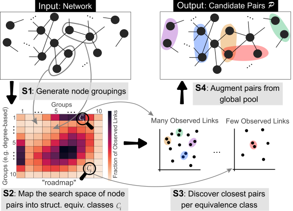
Figure 1: Our proposed framework LinkWaldo chooses candidate pairs from the quadratic, highly-skewed search space of possible links by first constructing a roadmap, which partitions the search space into structural equivalence classes of node pairs to capture how much pairs in each location resemble the observed links. This roadmap tells LinkWaldo how closely to look in each section of the search space. LinkWaldo follows the roadmap, selecting from each equivalence class the node pairs in closest proximity.

Link prediction is often evaluated via a ranking, where pairs of nodes that are not currently linked are sorted based on the “likelihood” score given by the method being evaluated [16]. To construct the ranking, a “ground-truth” test set of node pairs is constructed by either (1) removing a certain percentage of links from a graph at random or (2) removing the newest links that formed in the graph, if edges have timestamps. These removed edges form the test positives, and the same number of unlinked pairs are generated at random as test negatives. The methods are then evaluated on how well they are able to rank the test positives higher than the test negatives.

However, when link prediction is applied in practice, these ground truth labels are not known, since that is the very question that link prediction is attempting to answer. Instead, any pair of nodes that are not currently linked could link in the future. Thus, to identify likely missing or future links, a link prediction method would need to consider $O(n^{2})$ node pairs for a graph with $n$ nodes; most of which in sparse, real-world networks would turn out to not link. Proximity, on its own, is only a weak signal, sufficient to rank pairs in a balanced test set, but likely to turn up many false positives in an asymptotically skewed space, leaving discovering the relatively small number of missing or future links a challenging problem.

Proximity-based link prediction heuristics [15], such as Common Neighbors, could ignore some of the search space, such as nodes that are farther than two hops from each other, but this would not extend to other notions of proximity, like proximity-preserving embeddings. Duan et al. studied the problem of pruning the search space [5], but formulated it as top-$k$ link prediction, which attempts to predict a small number of links, but misses a large number of missing links in the process, suffering from low recall.

The goal of this work is to develop a principled approach to choose, from the quadratic and skewed space of possible links, a set of candidate pairs for a link prediction method to make decisions about. We envision that this will allow current and future developments to be realized for link prediction in practice, where no ground-truth set is available.

Problem 1.

Given a graph and a proximity function between nodes, we seek to return a candidate set of node pairs for a link predictor to make decisions about, such that the set is significantly smaller than the quadratic search space, but contains many of the missing and future links.

Our insight to handle the vast number of negatives is to consider not just the proximity of nodes, but also their structural resemblance to observed links. We measure resemblance as the fraction of observed links that fall in inferred, graph-structural equivalence classes of node pairs. For example, Fig. 1 shows one possible grouping of nodes based on their degrees, where the resulting structural equivalence classes (the cells in the “roadmap”) capture what fraction of observed links form between nodes of different degrees. Based on the roadmap, equivalence classes with a high fraction of observed edges are expected to contain more unlinked pairs than those with lower resemblance. We then employ node proximity within equivalence classes, rather than globally, which decreases false positives that are in close proximity, but do not resemble observed links, and decreases false negatives that are farther away in the graph, but resemble many observed edges. Moreover, to avoid computing proximities for all pairs of nodes within each equivalence class, we extend self-tuning locality sensitive hashing (LSH). Our main contributions are:

• Formulation & Theoretical Connections. Going beyond the heuristic of proximity between nodes, we model the plausibility of a node pair being linked as both their proximity and their structural resemblance to observed links. Based on this insight, we propose Future Link Location Models (FLLM), which combine Proximity Models and Stochastic Block Models; and we prove that Proximity Models are a naive special case. § III

• Scalable Method. We develop a scalable method, LinkWaldo (Fig. 1), which implements FLLM, and uses locality sensitive hashing to implicitly ignore unimportant pairs. § IV

• Empirical Analysis. We evaluate LinkWaldo on 13 diverse datasets from different domains, where it returns on average 22-33% more missing links than embedding-based models and 7-30% more than strong heuristics. § V

Our code is at https://github.com/GemsLab/LinkWaldo.

II Related work

In this paper, we focus on the understudied problem of choosing candidate pairs from the quadratic space of possible links, for link prediction methods to make predictions about. Link prediction techniques range from heuristic definitions of similarity, such as Common Neighbors [15], Jaccard Similarity [15], and Adamic-Adar [1], to machine learning approaches, such as latent methods, which learn low-dimensional node representations that preserve graph-structural proximity in latent space [7], and GNN methods, which learn heuristics specific to each graph [29] or attempt to re-construct the observed adjacency matrix [10]. For detailed discussion of link prediction techniques, we refer readers to [15] and [16].

Selecting Candidate Pairs. The closest problem to ours is top-$k$ link prediction [5], which attempts to take a particular link prediction method and prune its search space to directly return the $k$ highest score pairs. One method [5] samples multiple subgraphs to form a bagging ensemble, and performs NMF on each subgraph, returning the nodes with the largest latent factor products from each, while leveraging early-stopping. The authors view their method’s output as predictions rather than candidates, and thus focus on high precision at small values of $k$ relative to our setting. Another approach, Approximate Resistance Distance Link Predictor [21] generates spectral node embeddings by constructing a low-rank approximation of the graph’s effective resistance matrix, and applies a $k$-closest pairs algorithm on the embeddings, predicting these as links. However, this approach does not scale to moderate embedding dimensions (e.g., the dimensionality of 128 often-used used in embedding methods), and is often outperformed by the simple common neighbors heuristic.

A related problem is link-recommendation, which seeks to identify the $k$ most relevant nodes to a query node. It has been studied in social networks for friend recommendation [26], and in knowledge graphs [9] to pick subgraphs that are likely to contain links to a given query entity. In contrast, we focus on candidate pairs globally, not specific to a query node.

III Theory

Table I: Description of major symbols.

Notation	Description
$\mathcal{G}=(\mathcal{V},\mathcal{E}),\mathbf{A}$	Graph, nodes, edges, adjacency matrix
$|\mathcal{V}|=n,|\mathcal{E}|=m$	Number of nodes resp. edges in $\mathcal{G}$
$\mathcal{E}_{\text{new}}$	Unobserved future or missing links
$\Gamma$, $\Pi$	Grouping of $\mathcal{V}$, Partition of $\mathcal{V}\times\mathcal{V}$
$\mathbf{x}_{v}\in\mathbf{X},\bm{\mu}_{v}$	Node embedding and membership vector
$\mathcal{C}_{i}$	Equivalence class $i$
$\mathcal{P}$, $\tilde{\mathcal{P}}_{G}$	Pairs selected by LinkWaldo, global pool
$k,\kappa$	Budget for $|\mathcal{P}|$, target for an equiv. class

Let $\mathcal{G}=(\mathcal{V},\mathcal{E})$ be a graph or network with $|\mathcal{V}|=n$ nodes and $|\mathcal{E}|=m$ edges, where $\mathcal{E}\subseteq\mathcal{V}\times\mathcal{V}$. The adjacency matrix $\mathbf{A}$ of $\mathcal{G}$ is an $n\times n$ binary matrix with element $a_{ij}=1$ if nodes $i$ and $j$ are linked, and 0 otherwise. The set of node $v$’s neighbors is $\mathcal{N}(v)=\{u:(u,v)\in\mathcal{E}\}$. We summarize the key symbols used in this paper and their descriptions in Table I.

We now formalize the problem that we seek to solve:

Problem 2.

Given a graph $\mathcal{G}=(\mathcal{V},\mathcal{E})$, a proximity function $sim:\mathcal{V}\times\mathcal{V}\rightarrow\mathbb{R}^{+}$ between nodes, and a budget $k<<n^{2}$, return a set of plausible candidate node pairs $\mathcal{P}\subset\mathcal{V}\times\mathcal{V}$ of size $|\mathcal{P}|=k$ for a link predictor to make decisions about.

We describe next how to define resemblance in a principled way inspired by Stochastic Block Models, introduce a unified model for link prediction methods that use the proximity of nodes to rank pairs, and describe our model, which combines resemblance and proximity to solve Problem 2.

III-A Stochastic Block Models

Stochastic Block Models (SBMs) are generative models of networks. They model the connectivity of graphs as emerging from the community or group membership of nodes [20].

Node Grouping. A node grouping $\Gamma$ is a set of groups or subsets $\mathcal{V}_{i}$ of the nodes that satisfies $\bigcup_{\mathcal{V}_{i}\in\Gamma}\mathcal{V}_{i}=\mathcal{V}$. It is called a partition if it satisfies $\mathcal{V}_{i}\cap\mathcal{V}_{j}=\emptyset\;\;\forall\mathcal{V}_{i}\neq\mathcal{V}_{j}\in\Gamma$. Each node $v\in\mathcal{V}$ has a $|\Gamma|$-dimensional binary membership vector $\bm{\mu}_{v}$, with element $\mu_{vi}=1$ if $v$ belongs to group $\mathcal{V}_{i}$.

A node grouping can capture community structure, but it can also capture other graph-structural properties, like the degrees of nodes, in which case the SBM captures the compatibility of nodes w.r.t degree—viz. degree assortativity.

Membership Indices. The membership indices $I_{u,v}$ of nodes $u,v$ are the set of group ids $(i,j)$ s.t. $u\in\mathcal{V}_{i}$ and $v\in\mathcal{V}_{j}$: $I_{u,v}\triangleq\{i:\mu_{u,i}=1\}\times\{j:\mu_{v,j}=1\}$,   $i,j\in\{1,2,\dots,|\Gamma|\}$.

Membership equivalence relation & classes. The membership indices form the equivalence relation $\sim_{I}$: $(u,v)\sim_{I}(u^{\prime},v^{\prime})\iff I_{u,v}=I_{u^{\prime},v^{\prime}}$. This induces a partition $\Pi=\{\mathcal{C}_{1},\allowbreak\mathcal{C}_{2},\dots,\allowbreak\mathcal{C}_{|\Pi|}\}$ over all pairs of nodes $\mathcal{V}\times\mathcal{V}$ (both linked and unlinked), where the equivalence class $\mathcal{C}_{i}$ contains all node pairs $(u,v)$ with the same membership indices, i.e., $\bm{\mu}_{u}=\bm{\mu}$ and $\bm{\mu}_{v}=\bm{\mu}^{\prime}$ for some $\bm{\mu},\bm{\mu}^{\prime}\in\{0,1\}^{|\Gamma|}$. We denote the equivalence class of pair $(u,v)$ as $[(u,v)]_{\sim_{I}}$.

Example 1.

If nodes are grouped by their degrees to form $\Gamma$, then the membership indices $I_{u,v}$ of node pair $(u,v)$ are determined by $u$ and $v$’s respective degrees. For example, in Fig. 1, the upper circled node pair has degrees $3$ and $5$ respectively, which determines their equivalence class—in this case, the cell $(3,5)$ in the roadmap. Each cell of the roadmap corresponds to an equivalence class $\mathcal{C}_{i}\in\Pi$.

We can now formally define an SBM:

Definition 1 (Stochastic Block Model - SBM).

Given a node grouping $\Gamma$ and a $|\Gamma|\times|\Gamma|$ weight matrix $\mathbf{W}$ specifying the propensity for links to form across groups, the probability that two nodes link given their group memberships is $\text{Pr}(a_{uv}=1|\bm{\mu}_{u},\bm{\mu}_{v})=\sigma(\bm{\mu}_{u}^{T}\mathbf{W}\bm{\mu}_{v})$, where function $\sigma(\cdot)$ converts the dot product to a probability (e.g., sigmoid) [18].

The vanilla SBM [20] assigns each node to one group (i.e., the grouping is a partition and membership vectors $\bm{\mu}$ are one-hot), in which case $\bm{\mu}_{u}^{T}\mathbf{W}\bm{\mu}_{v}=w_{I_{u,v}}$. The overlapping SBM [18, 12] is a generalization that allows nodes to belong to multiple groups, in which case membership vectors may have multiple elements set to 1, and $\bm{\mu}_{u}^{T}\mathbf{W}\bm{\mu}_{v}=\sum_{i,j\in I_{u,v}}w_{ij}$.

Resemblance. Given an SBM with grouping $\Gamma$, we define the resemblance of node pair $(u,v)\in\mathcal{V}\times\mathcal{V}$ under the SBM as the percentage of the observed (training) edges that have the same group membership as $(u,v)$:

$${\rho}(u,v)\triangleq\frac{|\{(v_{1},v_{2})\in\mathcal{E}:(v_{1},v_{2})\sim_{I}(u,v)\}|}{m}.$$ (1)

Example 2.

In Figure 1, the resemblance ${\rho}(u,v)$ of node pair $(u,v)$ corresponds to the density of the cell that it maps to. The high density in the border cells indicates that many low-degree nodes connect to high-degree nodes. The dense central cells indicate that mid-degree nodes connect to each other.

III-B Proximity Models

Proximity-based link prediction models (PM) model the connectivity of graphs based on the proximity of nodes. Some methods define the proximity of nodes with a heuristic, such as Common Neighbors (CN), Jaccard Similarity (JS), and Adamic/Adar (AA). More recent approaches learn latent similarities between nodes, capturing the proximity in latent embeddings such that nodes that are in close proximity in the graph have similar latent embeddings (e.g., dot product) [7].

Node Embedding. A node embedding, $\mathbf{x}_{v}\in\mathbb{R}^{d}$, is a real-valued, $d$-dimensional vector representation of a node $v\in\mathcal{V}$. We denote all the node embeddings as matrix $\mathbf{X}\in\mathbb{R}^{n\times d}$.

Definition 2 (Proximity Model - PM).

Given a similarity or proximity function $sim:\mathcal{V}\times\mathcal{V}\rightarrow\mathbb{R}^{+}$ between nodes, the probability that nodes $u$ and $v$ link is an increasing function of their proximity: $\text{Pr}(a_{uv}=1|sim(\cdot,\cdot))=f(sim(u,v))$.

Instances of the PM include the Latent Proximity Model:

$$sim_{\text{LaPM}}(u,v)\triangleq\mathbf{x}_{u}^{T}\mathbf{x}_{v},$$ (2)

where $\mathbf{x}_{u},\mathbf{x}_{v}$ are the nodes’ latent embeddings; and the Common Neighbors, Jaccard Similarity, and Adamic/Adar models:

$$sim_{\textsc{CN}}(u,v)\triangleq|\mathcal{N}(u)\cap\mathcal{N}(v)|,$$ (3)

$$sim_{\textsc{JS}}(u,v)\triangleq\frac{|\mathcal{N}(u)\cap\mathcal{N}(v)|}{|\mathcal{N}(u)\cup\mathcal{N}(v)|},\text{ and}$$ (4)

$$sim_{\textsc{AA}}(u,v)\triangleq\sum_{v^{\prime}\in\mathcal{N}(u)\cap\mathcal{N}(v)}\frac{1}{\log|\mathcal{N}(v^{\prime})|}.$$ (5)

III-C Proposed: Future Link Location Model

Unlike SBM and PM, our model, which we call the Future Link Location Model (FLLM), is not just modeling the probability of links, but rather where in the search space future links are likely to fall. To do so, FLLM uses a partition of the search space, and corresponding SBM, as a roadmap that gives the number of new edges expected to fall in each equivalence class. To formalize this idea, we first define two distributions:

New and Observed Distributions. The new link distribution $p_{\text{n}}(\mathcal{C}_{i})\triangleq\text{Pr}(\mathcal{C}_{i}|\mathcal{E}_{\text{new}})$ and the observed link distribution $p_{\text{o}}(\mathcal{C}_{i})\triangleq\text{Pr}(\mathcal{C}_{i}|\mathcal{E})$ capture the fraction of new and observed edges that fall in equivalence class $\mathcal{C}_{i}$, respectively.

Definition 3 (Future Link Location Model - FLLM).

Given an overlapping SBM with grouping $\Gamma$, the expected number of new links in equivalence class $\mathcal{C}_{i}$ is proportional to the number of observed links in $\mathcal{C}_{i}$, and the probability of node pair $(u,v)$ linking is equal to the pair’s resemblance times their proximity relative to other nodes in $[(u,v)]_{\sim_{I}}$: $\text{Pr}(a_{uv}=1|\bm{\mu}_{u},\bm{\mu}_{v},sim(\cdot,\cdot))={\rho}(u,v)\cdot\frac{sim(u,v)}{\sum_{(u^{\prime},v^{\prime})\in[(u,v)]_{\sim_{I}}}sim(u^{\prime},v^{\prime})}$ .

FLLM employs the following theorem, which states that if $q\%$ of the observed links fall in equivalence class $\mathcal{C}_{i}$, then in expectation, $q\%$ of the unobserved links will fall in equivalence class $\mathcal{C}_{i}$. We initially assume that the unobserved future links follow the same distribution as the observed links—as generally assumed in machine learning—i.e., the relative fraction of links in each equivalence class will be the same for future links as observed links: $p_{\text{n}}=p_{\text{o}}$. In the next subsection, we show that for a fixed $k$, the error in this assumption is determined by the total variation distance between $p_{\text{n}}$ and $p_{\text{o}}$, and hence is upper-bounded by a constant.

Theorem 1.

Given an overlapping SBM with grouping $\Gamma$ inducing the partition $\Pi$ of $\mathcal{V}\times\mathcal{V}$ for a graph $\mathcal{G}=(\mathcal{V},\mathcal{E})$, out of $k$ new (unobserved) links $\mathcal{E}_{\text{new}}$, the expected number that will fall in equivalence class $\mathcal{C}_{i}$ and its variance are:

$$\mathbb{E}[|\mathcal{C}_{i}\cap\mathcal{E}_{new}|]=\frac{k|\mathcal{C}_{i}\cap\mathcal{E}|}{m}$$ (6)

$$Var(|\mathcal{C}_{i}\cap\mathcal{E}_{\text{new}}|)=\frac{k|\mathcal{C}_{i}\cap\mathcal{E}||\mathcal{E}\setminus\mathcal{C}_{i}|}{m^{2}}.$$ (7)

Proof.

Observe that the number of the $k$ new edges that fall in equivalence class $\mathcal{C}_{i}$, i.e., $|\mathcal{C}_{i}\cap\mathcal{E}_{\text{new}}|$, is a binomial random variable over $k$ trials, with success probability $\text{Pr}(\mathcal{C}_{i}|\mathcal{E}_{\text{new}})$. Thus, the random variable’s expected value is

$$\mathbb{E}[|\mathcal{C}_{i}\cap\mathcal{E}_{\text{new}}|]=k\text{Pr}(\mathcal{C}_{i}|\mathcal{E}_{\text{new}}),$$ (8)

and its variance is

$$Var(|\mathcal{C}_{i}\cap\mathcal{E}_{\text{new}}|)=k\text{Pr}(\mathcal{C}_{i}|\mathcal{E}_{\text{new}})(1-\text{Pr}(\mathcal{C}_{i}|\mathcal{E}_{\text{new}})).$$ (9)

We can derive $\text{Pr}(\mathcal{C}_{i}|\mathcal{E}_{\text{new}})$ via $\text{Pr}(\mathcal{C}_{i}|\mathcal{E})$ and Bayes’ rule:

$$\text{Pr}(\mathcal{C}_{i}|\mathcal{E})=\frac{\text{Pr}(\mathcal{E}|\mathcal{C}_{i})\text{Pr}(\mathcal{C}_{i})}{\text{Pr}(\mathcal{E})}=\frac{\frac{|\mathcal{C}_{i}\cap\mathcal{E}|}{|\mathcal{C}_{i}|}\frac{|\mathcal{C}_{i}|}{|\mathcal{V}\times\mathcal{V}|}}{m/|\mathcal{V}\times\mathcal{V}|}=\frac{|\mathcal{C}_{i}\cap\mathcal{E}|}{m}.$$

Combining the last equation with Eq. (8) results directly in Eq. (6), and by substituting into Eq. (9) we obtain:

$$Var(|\mathcal{C}_{i}\cap\mathcal{E}_{\text{new}}|)=\frac{k|\mathcal{C}_{i}\cap\mathcal{E}|}{m}(1-\frac{|\mathcal{C}_{i}\cap\mathcal{E}|}{m})=\frac{k|\mathcal{C}_{i}\cap\mathcal{E}||\mathcal{E}\setminus\mathcal{C}_{i}|}{m^{2}},$$

where we used the fact that $|\mathcal{E}\setminus\mathcal{C}_{i}|=|\mathcal{E}|-|\mathcal{C}_{i}\cap\mathcal{E}|$. ∎

III-D Guarantees on Error

While this derivation assumed that the future link distribution is the same as the observed link distribution, we now show that for a fixed $k$, the amount of error incurred when this assumption does not hold is entirely dependent on the total variation distance, and hence is upper-bounded by $2k$.

Total Variation Distance. The total variation distance [27] between $p_{\text{n}}$ and $p_{\text{o}}$, which is a metric, is defined as

$$d_{TV}(p_{\text{n}},p_{\text{o}})\triangleq\sup_{\mathcal{A}\subset\Pi}|p_{\text{n}}(\mathcal{A})-p_{\text{o}}(\mathcal{A})|.$$ (10)

Total Error. The total error made in the approximation of $\mathbb{E}[|\mathcal{C}_{i}\cap\mathcal{E}_{\text{new}}|]$ using Eq. (6) is defined as

$$\xi \triangleq\sum_{\mathcal{C}_{i}\in\Pi}|\hat{\mathbb{E}}[|\mathcal{C}_{i}\cap\mathcal{E}_{\text{new}}|]-\mathbb{E}[|\mathcal{C}_{i}\cap\mathcal{E}_{\text{new}}|]|$$

$$=\sum_{\mathcal{C}_{i}\in\Pi}|kp_{\text{o}}(\mathcal{C}_{i})-kp_{\text{n}}(\mathcal{C}_{i})|,$$ (11)

where $\hat{\mathbb{E}}[|\mathcal{C}_{i}\cap\mathcal{E}_{\text{new}}|]$ is the true expected value regardless of whether or not $p_{\text{n}}=p_{\text{o}}$ holds.

Theorem 2.

The total error incurred over $\Pi$ in the computation of the expected number of new edges that fall in each $\mathcal{C}_{i}\in\Pi$ is an increasing function of the the number of new pairs $k$ and the total variation distance between $p_{\text{n}}$ and $p_{\text{o}}$. Furthermore, it has the following upper-bound:

$$\xi=2k\,d_{TV}(p_{\text{n}},p_{\text{o}})\leq\min(2k,2k\sqrt{1/2D_{\text{KL}}(p_{\text{n}}||p_{\text{o}})}).$$ (12)

Proof.

From the definition of total error in Eq. (11), the first equality holds from [14]. The inequality holds based on the fact that $d_{TV}(\cdot,\cdot)$ ranges in $[0,1]$, and Pinsker’s inequality [27], which upper-bounds $d_{TV}(\cdot,\cdot)$ via KL-divergence. ∎

III-E Proximity Model as a Special Case of FLLM

The PM, defined in § III-B, is a special case of FLLM, where FLLM’s grouping contains just one group $\Gamma=\{\mathcal{V}\}$. That is, if the nodes are not grouped, then the models give the same result. Thus, FLLM’s improvement over LaPM is a result of using structurally-meaningful groupings over the graph. The following theorem states this result formally.

Theorem 3.

For a single node grouping $\Gamma=\{\mathcal{V}\}$, both PM and FLLM give the same ranking of pairs $(u,v)\in\mathcal{V}\times\mathcal{V}$:

$$\text{Pr}_{\text{PM}}(a_{uv}=1|sim(\cdot,\cdot)) >\text{Pr}_{\text{PM}}(a_{u^{\prime}v^{\prime}}=1|sim(\cdot,\cdot))\iff$$

$$\text{Pr}_{\text{FLLM}}(a_{uv}=1|\bm{\mu}_{u},\bm{\mu}_{v},sim(\cdot,\cdot)) >\text{Pr}_{\text{FLLM}}(a_{u^{\prime}v^{\prime}}=1|\bm{\mu}_{u^{\prime}},\bm{\mu}_{v^{\prime}},sim(\cdot,\cdot)).$$

Proof.

Since $\Gamma=\{\mathcal{V}\}$, $\Pi=\{\mathcal{V}\times\mathcal{V}\}$, and since $\mathcal{E}\subseteq\mathcal{V}\times\mathcal{V}$, all observed edges fall in the lone equivalence class $\mathcal{C}=\mathcal{V}\times\mathcal{V}$. Thus ${\rho}(u,v)=1\ \forall(u,v)\in\mathcal{V}\times\mathcal{V}$. Since there is only one equivalence class, the denominator in Dfn. 3 is equal to a constant $c\triangleq\sum_{(u^{\prime},v^{\prime})\in[(u,v)]_{\sim_{I}}}sim(u^{\prime},v^{\prime})=\sum_{(u^{\prime},v^{\prime})\in\mathcal{V}\times\mathcal{V}}sim(u^{\prime},v^{\prime})\ \forall(u,v)\in\mathcal{V}\times\mathcal{V}$. Therefore, $\text{Pr}_{\text{FLLM}}(a_{uv}=1|\bm{\mu}_{u},\bm{\mu}_{v},sim(\cdot,\cdot))=\frac{1}{c}sim(u,v)$, and both models are increasing functions of $sim(\cdot,\cdot)$. ∎

IV Method

We solve Problem 2 by using our FLLM model in a new method, LinkWaldo, shown in Fig. 1, which has four steps:

• S1: Generate node groupings and equivalence classes.

• S2: Map the search space, deciding how many candidate pairs to return from each equivalence class.

• S3: Search each equivalence class, returning directly the highest-proximity pairs, and stashing some slightly lower-proximity pairs in a global pool.

• S4: Choose the best pairs from the global pool to augment those returned from each equivalence class.

We discuss these steps next, give pseudocode in Alg. 1, and discuss time complexity in the appendix.

IV-A Generating Node Groupings (S1)

In theory, we would like to infer the groupings that directly maximize the likelihood of the observed adjacency matrix. However, the techniques for inferring these groupings (and the corresponding node membership vectors) are computationally intensive, relying on Markov chain Monte Carlo (MCMC) methods [17]. Indeed, these methods are generally applied in networks with only up to a few hundred nodes [18]. In cases where $n$ is large enough that considering all $O(n^{2})$ node pairs would be computationally infeasible, so would be MCMC. Instead LinkWaldo uses a fixed grouping, though it is agnostic to how the nodes are grouped. We discuss a number of sensible groupings below, and discuss how to set the number of groups in § V-D. Any other grouping can be readily used within our framework, but should be carefully chosen to lead to strong results.

$\bullet$ Log-binned Node Degree (DG). This grouping captures degree assortativity [19], i.e., the extent to which low degree nodes link with other low degree nodes vs. high degree nodes, by creating uniform bins in log-space (e.g., Fig. 1; linear bins).

$\bullet$ Structural Embedding Clusters (SG). This grouping extends DG by clustering latent node embeddings that capture structural roles of nodes [24].

$\bullet$ Communities (CG). This grouping captures community structure by clustering proximity preserving latent embeddings or using community detection methods.

$\bullet$ Multiple Groupings (MG). Any subset of these groupings or any other groupings can be combined into a new grouping, by setting $\bm{\mu}_{v}$ element(s) to 1 for $v$’s membership in each grouping, since nodes can have overlapping group memberships.

Algorithm 1 LinkWaldo($\mathcal{G}$, $sim(\cdot,\cdot)$, $k,\tau$)

1:/* S1: Generating Node Groupings */

2:Generate node grouping $\Gamma$ inducing partition $\Pi$ $\triangleright$ § IV-A

3:$\mathcal{P},\tilde{\mathcal{P}}_{G}\leftarrow\emptyset,\emptyset$ $\triangleright$ Initialize pairs to return and global pool

4:for $\mathcal{C}_{i}\in\Pi$ do $\triangleright$ Search each equivalence class § IV-C

5:   /* S2: Mapping the Search Space */

6:   $\bar{\mu}\leftarrow\mathbb{E}[|\mathcal{C}_{i}\cap\mathcal{E}_{\text{new}}|]$ $\triangleright$ Eq. (6)

7:   $\sigma\leftarrow\sqrt{Var(|\mathcal{C}_{i}\cap\mathcal{E}_{\text{new}}|)}$ $\triangleright$ Eq. (7)

8:   /* S3: Discovering Closest Pairs per Equivalence Class */

9:   if $|\mathcal{C}_{i}|<\tau$ then

10:     $\textsc{SelectPairsExact}(\mathcal{P},\tilde{\mathcal{P}}_{G},\mathcal{C}_{i},\bar{\mu},\sigma)$

11:   else

12:     $\textsc{SelectPairsApprox}(\mathcal{P},\tilde{\mathcal{P}}_{G},\mathcal{C}_{i},\bar{\mu},\sigma)$    

13:/* S4: Augmenting Pairs from Global Pool */

14:$\mathcal{P}\leftarrow$   $\mathcal{P}\cup\{\text{top }k-|\mathcal{P}|\text{ pairs from }\tilde{\mathcal{P}}_{G}\}$

15:return $\mathcal{P}$

16:procedure SelectPairsExact($\mathcal{P}$, $\tilde{\mathcal{P}}_{G}$, $\mathcal{C}_{i}$, $\bar{\mu}$, $\sigma$)

17:   Sort pairs $(u,v)\in\mathcal{C}_{i}$ in descending order on $sim(u,v)$

18:   $\mathcal{P}\leftarrow$ $\mathcal{P}\cup$ {top $\bar{\mu}-\sigma$ pairs}

19:   $\tilde{\mathcal{P}}_{G}\leftarrow\tilde{\mathcal{P}}_{G}\cup$ {next $2\sigma$ pairs}

20:procedure SelectPairsApprox($\mathcal{P}$, $\tilde{\mathcal{P}}_{G}$, $\mathcal{C}_{i}$, $\bar{\mu}$, $\sigma$)

21:   for $i=1,2,\dots,r$ do $\triangleright$ Create $r$ trees

22:     $\mathcal{B}\leftarrow\{(\mathcal{V}_{u},\mathcal{V}_{v})\}$ $\triangleright$ buckets start off as the root

23:     while $\text{Vol}(\mathcal{B})>\kappa$ do $\triangleright$ cf. Prob. 3 for $\kappa$ definition

24:       Choose $h(\cdot)$ at random from $\mathcal{H}_{\text{rh}}$

25:       $\mathcal{B}^{\prime}\leftarrow\emptyset$ $\triangleright$ Create new buckets

26:       for $\beta\in\mathcal{B}$ do $\triangleright$ Branch each leaf (bucket)

27:         $\beta_{\text{left}}^{\prime}\leftarrow$

$(\{u\in\mathcal{V}_{u}^{(\beta)}:h(\mathbf{x}_{u})<0\},\{v\in\mathcal{V}_{v}^{(\beta)}:h(\mathbf{x}_{v})<0\})$

28:         $\beta_{\text{right}}^{\prime}\leftarrow$

$(\{u\in\mathcal{V}_{u}^{(\beta)}:h(\mathbf{x}_{u})\geq 0\},\{v\in\mathcal{V}_{v}^{(\beta)}:h(\mathbf{x}_{v})\geq 0\})$

29:         $\mathcal{B}^{\prime}\leftarrow\mathcal{B}^{\prime}\cup\{\beta_{\text{left}},\beta_{\text{right}}\}$        

30:       if $\text{Vol}(\mathcal{B})\leq\kappa$ then $\mathcal{B}\leftarrow\mathcal{B}^{\prime}$                

31:   $\mathcal{P}\leftarrow$ $\mathcal{P}\cup$ {top $\bar{\mu}-\sigma$ pairs}

32:   $\tilde{\mathcal{P}}_{G}\leftarrow\tilde{\mathcal{P}}_{G}\cup$ {next $2\sigma$ pairs}

IV-B Mapping the Search Space (S2)

LinkWaldo’s approach to mapping the search space (i.e., identifying how many pairs to return per class $\mathcal{C}_{i}$) follows directly from Thm. 1. LinkWaldo computes the expected number of pairs in each equivalence class based on Eq. (6) and its variance based on Eq. (7), as a measure of the uncertainty. When LinkWaldo searches each equivalence class $\mathcal{C}_{i}$, it returns the expected number of pairs minus a standard deviation directly, and adds more pairs, up to a standard deviation past the mean, to a global pool $\tilde{\mathcal{P}}_{G}$. Thus, LinkWaldo adds into $\mathcal{P}$ the $\mathbb{E}[|\mathcal{C}_{i}\cap\mathcal{E}_{new}|]-\sqrt{Var(|\mathcal{C}_{i}\cap\mathcal{E}_{\text{new}}|)}$ pairs in closest proximity in equivalence class $\mathcal{C}_{i}$, and the next $2\sqrt{Var(|\mathcal{C}_{i}\cap\mathcal{E}_{\text{new}}|)}$ closest pairs into the global pool $\tilde{\mathcal{P}}_{G}$ (both expressions are rounded to the nearest integer). Node pairs that are already linked are skipped.

IV-C Discovering Closest Pairs per Equivalence Class (S3)

We now discuss how LinkWaldo discovers the $\kappa$ closest unlinked pairs within each equivalence class (Fig. 1), where $\kappa$ is determined in step S2 based on the expected number of pairs in the equivalence class, and variance (uncertainty).

Problem 3.

Given an equivalence class $\mathcal{C}_{i}$, return the top-$\kappa$ unlinked pairs in $\mathcal{C}_{i}$ in closest proximity $sim(\cdot,\cdot)$, where $\kappa=\mathbb{E}[|\mathcal{C}_{i}\cap\mathcal{E}_{new}|]+\sqrt{Var(|\mathcal{C}_{i}\cap\mathcal{E}_{\text{new}}|)}$ (based on S2).

For equivalence classes smaller than some tolerance $\tau$, it is feasible to search all pairs of nodes exhaustively. However, for $|\mathcal{C}_{i}|>\tau$, this should be avoided, to make the search practical. We first discuss this case when using the dot product similarity $sim_{\text{LaPM}}(\cdot,\cdot)$ in Eq. (2), and then discuss it for other similarity models (CN, JS, and AA) given by Eqs. (3)-(5). Finally, we introduce a refinement that improves the robustness of LinkWaldo against errors in proximity.

IV-C1 Avoiding Exhaustive Search for Dot Product

In the case of dot product, we use Locality Sensitive Hashing (LSH) [28] to avoid searching all $|\mathcal{C}_{i}|$ pairs. LSH functions have the property that the probability of two items colliding is a function of their similarity. We use the following fact:

Fact 1.

The equivalence class $\mathcal{C}_{i}$ can be decomposed into the Cartesian product of two sets $\mathcal{C}_{i}=\mathcal{V}_{u}\times\mathcal{V}_{v}$, where $\mathcal{V}_{u}\triangleq\{u:\bm{\mu}_{u}=\bm{\mu}\}$ and $\mathcal{V}_{v}=\{v:\bm{\mu}_{v}=\bm{\mu}^{\prime}\}$.

At a high level, to solve Prob. 3, we hash each node embedding of the nodes in $\mathcal{V}_{u}$ and $\mathcal{V}_{v}$ using a locality sensitive hash function. We design the hash function, described next, such that the number of pairs that map to the same bucket is greater than $\kappa$, but as small as possible, to maximally prune pairs. Once the embeddings are hashed, we search the pairs in each hash bucket for the $\kappa$ closest. We normalize the embeddings so that dot product is equivalent to cosine similarity, and use the Random Hyperplane LSH family [4].

Definition 4 (Random Hyperplane Hash Family).

The random hyperplane hash family $\mathcal{H}_{\text{rh}}$ is the set of hash functions $\mathcal{H}_{\text{rh}}\triangleq\{h:\mathbb{R}^{d}\rightarrow\{0,1\}\}$, where $\mathbf{r}_{h}$ is a random $d$-dimensional Gaussian unit vector and $h(\mathbf{x})\triangleq\begin{cases}1&\text{if }\mathbf{r}_{h}^{T}\mathbf{x}\geq 0\\ 0&\text{if }\mathbf{r}_{h}^{T}\mathbf{x}<0\end{cases}$.

This hash family is well-known to provide the property that the probability of two vectors colliding is a function of the degree of the angle between them [2]:

$$\small\text{Pr}(h(\mathbf{x}_{u})=h(\mathbf{x}_{v}))=1-\frac{\theta(\mathbf{x}_{u},\mathbf{x}_{v})}{\pi}=1-\frac{\arccos(\mathbf{x}_{u}^{T}\mathbf{x}_{v})}{\pi},$$

where the last equality holds due to normalized embeddings.

To lower the false positive rate, it is conventional to form a new hash function by sampling $b$ hash functions from $\mathcal{H}_{\text{rh}}$ and concatenating the hash codes: $g(\cdot)=(h_{1}(\cdot),h_{2}(\cdot),\dots,h_{b}(\cdot))$. The new hash function is from another LSH family:

Definition 5 ($b$-AND-Random Hyperplane Hash Family).

The $b$-AND-Random hyperplane hash family is the set of hash functions $\mathcal{H}_{\text{and}}^{b}\triangleq\{g:\mathbb{R}^{d}\rightarrow\{0,1\}^{b}\}$, where $g(\mathbf{x})=(h_{1}(\mathbf{x}),h_{2}(\mathbf{x}),\dots,h_{b}(\mathbf{x}))$ is formed by concatenating $b$ randomly sampled hash functions $h(\cdot)\in\mathcal{H}_{\text{rh}}$ for some $b\in\mathbb{N}$.

Since the hash functions are sampled randomly from $\mathcal{H}_{\text{rh}}$,

$$\small\text{Pr}(g(\mathbf{x}_{u})=g(\mathbf{x}_{v}))=\left(1-\frac{\arccos(\mathbf{x}_{u}^{T}\mathbf{x}_{v})}{\pi}\right)^{b}.$$

Only vectors that are not split by all $b$ random hyperplanes end up with the same hash codes, so this process lowers the false positive rate. However, it also increases the false negative rate for the same reason. The conventional LSH-scheme then repeats the process $r$ times, computing the dot product exactly over all pairs that match in at least one $b$-dim hash code, in order to lower the false negative rate. The challenge of this approach is determining how to set $b$. To do so, we first define the hash buckets of a hash function, and their volume.

Definition 6 (Hash Buckets and Volume).

Given an equivalence class $\mathcal{C}_{i}=\mathcal{V}_{u}\times\mathcal{V}_{v}$ and a hash function $g(\cdot):\mathbb{R}^{d}\rightarrow\{0,1\}^{b}$, after applying $g(\cdot)$ to all $v\in\mathcal{V}_{u}\cup\mathcal{V}_{v}$, a hash bucket

$$\beta=\{u\in\mathcal{V}_{u},v\in\mathcal{V}_{v}:g(u)=g(v)=\beta_{\text{hashcode}}\}$$

consists of subsets $\mathcal{V}_{u}^{(\beta)}\subseteq\mathcal{V}_{u},\mathcal{V}_{v}^{(\beta)}\subseteq\mathcal{V}_{v}$ of nodes that mapped to hashcode $\beta_{\text{hashcode}}\in\{0,1\}^{b}$. The set of hash buckets $\mathcal{B}_{g}=\{\beta:|\beta|>0\}$ consists of all non-empty buckets. We define the volume of the buckets as the number of pairs $(u,v)$ where $u$ and $v$ landed in the same bucket:

$$\small\text{Vol}(\mathcal{B}_{g})\triangleq|\{(u,v):g(\mathbf{x}_{u})=g(\mathbf{x}_{v})\}|=\textstyle\sum_{\beta\in\mathcal{B}_{g}}|\mathcal{V}_{u}^{(\beta)}\times\mathcal{V}_{v}^{(\beta)}|.$$

Since we are after the $\kappa$ closest pairs, we want to find a hash function $g(\cdot)$ such that $\text{Vol}(\mathcal{B}_{g})\geq\kappa$. But since we want to search as few pairs as possible, we seek the value of $b$ that minimizes $\text{Vol}(\mathcal{B}_{g})$ for some $g(\cdot)\in\mathcal{H}_{\text{and}}^{b}$ subject to the constraint that $\text{Vol}(\mathcal{B}_{g})\geq\kappa$.

Any hash function $g\in\mathcal{H}_{\text{and}}^{b}$ corresponds to a binary prefix tree, like Fig. 2. Each level of the tree corresponds to one

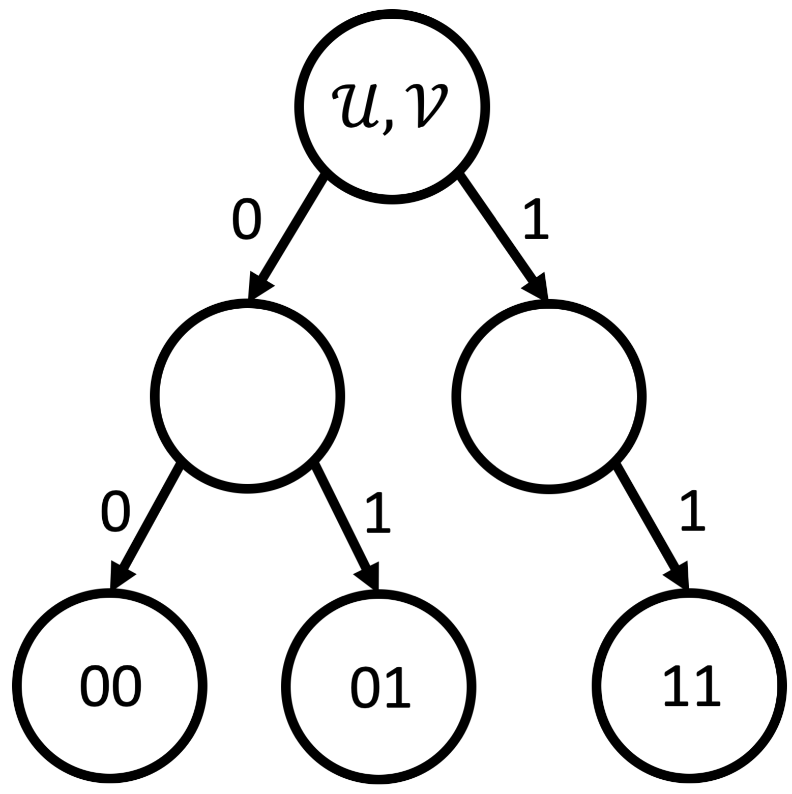
Figure 2: LSH Tree

$h\in\mathcal{H}_{\text{rh}}$, and the leaves correspond to the buckets $\mathcal{B}_{g}$. Thus, to automatically identify the best value of $b$, we can recursively grow the tree, branching each leaf with a new random hyperplane hash function $h\in\mathcal{H}_{\text{rh}}$, until $\text{Vol}(\mathcal{B}_{g})<\kappa$, then undo the last branch. At that point, the depth of the tree equals $b$, and is the largest value such that $\text{Vol}(\mathcal{B}_{g})\geq\kappa$. To prevent this process from repeating indefinitely in edge cases, we halt the branching at a maximum depth $b_{\max}$. This approach is closely related to LSH Forests [2], but with some key differences, which we discuss below.

Theorem 4.

Given a hash function $g\in\mathcal{H}_{\text{and}}^{b}$, the $\kappa$ closest pairs in $\mathcal{C}_{i}$ are the $\kappa$ most likely pairs to be in the same bucket: $\text{Pr}(g(\mathbf{x}_{u})=g(\mathbf{x}_{v}))>\text{Pr}(g(\mathbf{x}_{u^{\prime}})=g(\mathbf{x}_{v^{\prime}}))\iff\mathbf{x}_{u}^{T}\mathbf{x}_{v}>\mathbf{x}_{u^{\prime}}^{T}\mathbf{x}_{v^{\prime}}$ .

Proof.

Since $\arccos(x)$ is a decreasing function of $x$, Eq. (IV-C1) shows that $\text{Pr}(g(\mathbf{x}_{u})=g(\mathbf{x}_{v}))$ is an increasing function of $\mathbf{x}_{u}^{T}\mathbf{x}_{v}$. The result follows from this. ∎

While $\mathbf{x}_{u}^{T}\mathbf{x}_{v}>\mathbf{x}_{u^{\prime}}^{T}\mathbf{x}_{v^{\prime}}$ implies that $(u,v)$ are more likely than $(u^{\prime},v^{\prime})$ to be in the same bucket, it does not guarantee that this outcome will always happen. Thus, we repeat the process $r$ times, creating $r$ binary prefix trees and, searching the pairs that fall in the same bucket in any tree for the top $\kappa$. Setting the $r$ parameter is considered of minor importance, as long as it is sufficiently large (e.g., 10) [2].

Differences from LSH Forests [2]. LSH Forests are designed for $KNN$-search, which seeks to return the nearest neighbors to a query vector. In contrast, our approach is designed for $\kappa$-closest-pairs search, which seeks to return the $\kappa$ closest pairs in a set $\mathcal{C}_{i}$. LSH Forests grow each tree until each vector is in its own leaf. We grow each tree until we reach the target bucket volume $\kappa$. LSH Forests allow variable length hash codes, since the nearest neighbors of different query vectors may be at different relative distances. All our leaves are at the same depth so that the probability of $(u,v)$ surviving together to the leaf is an increasing function of their dot product.

IV-C2 Avoiding Exhaustive Search for Heuristics

For the heuristic definitions of proximity in Eqs.(3)-(5), there are two approaches to solving Prob. 3. The first is to construct embeddings from the CN and AA scores (this does not apply to JS). For CN, if we let the node embeddings be their corresponding rows in the adjacency matrix, i.e, $\mathbf{X}_{\textsc{CN}}=\mathbf{A}$, then $sim_{\textsc{CN}}(u,v)=\mathbf{x}_{u}^{T}\mathbf{x}_{v}$. Similarly, $\mathbf{X}_{\textsc{AA}}=\mathbf{A}\cdot 1/\sqrt{\log(\mathbf{D})}$, yields $sim_{\textsc{AA}}(u,v)=\mathbf{x}_{u}^{T}\mathbf{x}_{v}$, where $\mathbf{D}$ is a diagonal matrix recording the degree of each node. Thus, the LSH solution just described can be applied. The second approach uses the fact that all three heuristics are defined over the 1-hop neighborhoods of nodes $(u,v)$. Thus, to have nonzero proximity, $(u,v)$ must be within 2-hops of each other, and any pairs not within 2-hops can implicitly be ignored.

IV-C3 Bail Out Refinement

To this point we have assumed that the proximity model used in LinkWaldo is highly informative and accurate. However, in reality, heuristics may not be informative for all equivalence classes, and even learned, latent proximity models, can fail to encode adequate information. For instance, it is challenging to learn high-quality representations for low-degree nodes. Thus, we introduce a refinement to LinkWaldo that automatically identifies when a proximity model is uninformative in an equivalence class, and allows it to bail out of searching that equivalence class.

Proximity Model Error. The error that a proximity model makes is the probability $\text{Pr}(sim(u,v)<sim(u^{\prime},v^{\prime}))$ that it gives a higher proximity for some unlinked pair $(u^{\prime},v^{\prime})\notin\mathcal{E}$ than for some linked pair $(u,v)\in\mathcal{E}$.

By this definition of error, we expect strong proximity models to mostly assign higher proximity between observed edges than future or missing edges: $\text{Pr}(sim(u,v)>sim(u^{\prime},v^{\prime}))\approx 1$ for some $(u,v)\in\mathcal{E}$ and $(u^{\prime},v^{\prime})\in\mathcal{E}_{\text{new}}$. Thus, on our way to finding the top-$\kappa$ most similar (unlinked) pairs in an equivalence class (Problem 3), we expect to encounter a majority of the observed edges (linked pairs) $|\mathcal{E}\cap\mathcal{C}_{i}|$ that fall in that class. For a user-specified error tolerance $\zeta$, LinkWaldo will bail out and return no pairs from any equivalence class where less than $\zeta$ fraction of its observed edges are encountered on the way to finding the $\kappa$ most similar unlinked pairs. LinkWaldo keeps track of how many pairs were skipped by bailing out, and replaces them (after step S4) by adding to $\mathcal{P}$ the top-ranked pairs of a heuristic (e.g., AA).

IV-D Augmenting Pairs from Global Pool (S4)

Since LinkWaldo returns a standard deviation below the expected number of new pairs in each equivalence class, it chooses the remaining pairs up to $k$ from $\tilde{\mathcal{P}}_{G}$. To do so, it considers pairs in descending order on the input similarity function $sim(\cdot,\cdot)$, and greedily adds to $\mathcal{P}$ until $|\mathcal{P}|=k$.

V Evaluation

We evaluate LinkWaldo on three research questions: (RQ1) Does the set $\mathcal{P}$ returned by LinkWaldo have high recall and precision? (RQ2) Is LinkWaldo scalable? (RQ3) How do parameters affect performance?

Table II: Datasets statistics: if the graph is temporal or static, density, degree assortativity [19], and number of nodes and edges.

Graph	Time	Density	Assortativity	$n$	$m$
Yeast	-	0.41%	0.4539	2,375	11,693
DBLP	-	0.06%	-0.0458	12,595	49,638
Facebook1	-	1.08%	0.0636	4,041	88,235
MovieLens	✓	2.90%	-0.2268	2,627	100,000
HS-Protein	-	0.74%	0.2483	6,329	147,548
arXiv	-	0.11%	0.2051	18,772	198,110
MathOverflow	✓	0.06%	-0.1979	24,820	199,974
Enron	✓	0.01%	-0.1667	87,275	299,221
Reddit	✓	0.01%	-0.1278	67,180	309,667
Epinions	-	0.01%	-0.0406	75,881	405,741
Facebook2	✓	0.04%	0.1770	63,733	817,063
Digg	✓	$<0.01\%$	-0.0557	279,376	1,546,541
Protein-Soy	-	1.64%	-0.0192	45,116	16,691,679

V-A Data & Setup

We evaluate LinkWaldo on a large, diverse set of networks: metabolic, social, communication, and information networks. Moreover, we include datasets to evaluate in both LP scenarios: (1) returning possible missing links in static graphs and (2) returning possible future links in temporal graphs. We treat all graphs as undirected.

Metabolic. Yeast [29], HS-Protein [11], and Protein-Soy [13] are metabolic protein networks, where edges denote known associations between proteins in different species. Yeast contains proteins in a species of yeast, HS-Protein in human beings, and Protein-Soy in Glycine max (soybeans).

Social. Facebook1 [13] and Facebook2 [11] capture friendships on Facebook, Reddit [13] encodes links between subreddits (topical discussion boards), edges in Epinions [11] connect users who trust each other’s opinions, MathOverflow [13] captures comments and answers on math-related questions and comments (e.g., user $u$ answered user $v$’s question), Digg [23] captures friendships among users.

Communication. Enron [11] is an email network, capturing emails sent during the collapse of the Enron energy company.

Information. DBLP [11] is a citation network, and arXiv [13] is a co-authorship network of Astrophysicists. MovieLens [11] is bipartite graph of users rating movies for the research project MovieLens. Edges encode users and the movies that they rated.

Training Graph and Ground Truth. While using LinkWaldo in practice does not require a test set, in order to know how effective it is, we must evaluate it on ground truth missing links. As ground truth, we remove 20% of the edges. In the static graphs, we remove 20% at random. In the temporal graphs, we remove the 20% of edges with the most recent timestamps. If either of the nodes in the removed edge is not present in the training graph, we discard the edge from the ground-truth. The graph with these edges removed is the training graph, which LinkWaldo and the baselines observe when choosing the set of unlinked pairs to return.

Setup. We discuss in § V-D how we choose which groupings to use, and how many groups in each. Whenever used, we implement SG and CG by clustering embeddings with KMeans: xNetMF [8] and NetMF [22] (window size 1), respectively. In LSH, we set the maximum tree depth dynamically based on the size of an equivalence class: $b_{\max}=12$ if $|\mathcal{C}_{i}|<1B$, $b_{\max}=15$ if $|\mathcal{C}_{i}|<10B$, $b_{\max}=20$ $|\mathcal{C}_{i}|<25B$, $b_{\max}=30$ otherwise. We set the number of trees $r$ based on the fraction of $|\mathcal{C}_{i}|$ that we seek to return: $r=5$ if $\kappa/|\mathcal{C}_{i}|<0.0001$, $r=10$ if $\kappa/|\mathcal{C}_{i}|<0.001$ and $r=25$ otherwise.

V-B Recall and Precision (RQ1)

Task Setup. We evaluate how effectively LinkWaldo returns in $\mathcal{P}$ the ground-truth missing links, at values of $k$ much smaller than $n^{2}$. We report $k$, chosen based on dataset size, in Tab. III, and discuss effects of the choice in the appendix. We compare the set LinkWaldo returns to those of five baselines, and evaluate both LinkWaldo-D, which uses grouping DG, and LinkWaldo-M, which uses DG, SG, and CG together. In both LinkWaldo variants, we consider the following proximities (cf. III-B) as input, and report the results that are best: LaPM using NetMF [22] embeddings (window sizes 1 and 2), and AA, the best heuristic proximity. For the bipartite MovieLens, we use BiNE [6], an embedding method designed for bipartite graphs. We report the input proximity model for each dataset in Tab. V in the appendix. We set the exact-search and bailout tolerances to $\tau=25M$ and $\zeta=0.5$, which we determined via a parameter study in § V-D. Results are averages over five random seeds (§ V-A): for static graphs, the randomly-removed edges are different for each seed; for temporal graphs, the latest edges are always removed, so the LSH hash functions are the main source of randomness.

Metrics. We use Recall (R@$k$), the fraction of known missing/future links that are in the size-$k$ set returned by the method, and Precision (P@$k$), the fraction of the $k$ pairs that are known to be missing/future links. Recall is a more important metric, since (1) the returned set of pairs $\mathcal{P}$ does not contain final predictions, but rather pairs for a LP method to make final decisions about, and (2) our real-world graphs are inherently incomplete, and thus pairs returned that are not known to be missing links, could nonetheless be missing in the original dataset prior to ground-truth removal (i.e., the open-world assumption [25]). We report both in Table III.

Baselines. We use five baselines. NMF+Bag [5] uses non-negative matrix factorization (NMF) and a bagging ensemble to return $k$ pairs while pruning the search space. We use their reported strongest version: the Biased Edge Bagging version with Node Uptake and Edge Filter optimizations (Biased(NMF+)). We use the authors’ recommended parameters when possible: $\epsilon=1$, $\mu=0.1$, $f=0.1$, $\rho=0.75$, number of latent factors $d=50$, and ensemble size $\mu/f^{2}$. In some cases, these suggested parameters led to fewer than $k$ pairs being returned, in which case we tweaked the values of $\epsilon,\mu$, and $f$ until $k$ were returned. We report these deviations in Tab. V in the appendix. We use our own implementation.

We also use four proximity models, which we showed to be special cases of FLLM in § III-E: LaPM ranks pairs globally based on the dot product of their embeddings, and returns the top $k$. To avoid searching all-pairs, we use the same LSH scheme that we introduce in § IV-C for LinkWaldo. We set $r=25$, and like LinkWaldo, use NetMF with a window size of 1 or 2, except for MovieLens, where we use BiNE.

JS, CN, and AA are defined in III-B. We exploit the property described in IV-C2—i.e., all these scores are zero for nodes beyond two hops. We compute the scores for all nodes within two hops, and return the top $k$ unlinked pairs.

Table III: On each dataset, we highlight the cell of the top-performing method with bold text and a gray background, and the second best with bold text only. An “*” denotes statistical significance at a 0.05 $p$-value in a paired t-test. The “**” means that the difference between the better performing variant of LinkWaldo was also significantly better than the other variant at the same $p$-value. Under each dataset, we give the percentage of the quadratic search space that the value of $k$ corresponds to (usually $<1\%$). On average, LinkWaldo-M is the best-performing method, and LinkWaldo-D the second best.

Dataset	Metric	NMF+Bag [5]	LaPM	JS	CN	AA	LinkWaldo-D	LinkWaldo-M
Yeast	R@10K	0.4078 $\pm$ 0.01	0.4400 $\pm$ 0.01	0.4766 $\pm$ 0.01	0.6142 $\pm$ 0.01	0.6590 $\pm$ 0.01	0.6762 $\pm$ 0.01	0.6926** $\pm$ 0.01
0.39%	P@10K	0.0898 $\pm$ 0.00	0.0969 $\pm$ 0.00	0.1049 $\pm$ 0.00	0.1352 $\pm$ 0.00	0.1451 $\pm$ 0.00	0.1489 $\pm$ 0.00	0.1525** $\pm$ 0.00
DBLP	R@100K	0.2319 $\pm$ 0.00	0.0927 $\pm$ 0.00	0.0389 $\pm$ 0.00	0.3379 $\pm$ 0.00	0.3775 $\pm$ 0.00	0.4270 $\pm$ 0.00	0.4271* $\pm$ 0.00
0.15%	P@100K	0.0204 $\pm$ 0.00	0.0082 $\pm$ 0.00	0.0034 $\pm$ 0.00	0.0298 $\pm$ 0.00	0.0332 $\pm$ 0.00	0.0376* $\pm$ 0.00	0.0376* $\pm$ 0.00
Facebook1	R@100K	0.4036 $\pm$ 0.02	0.8005 $\pm$ 0.00	0.8244 $\pm$ 0.00	0.8547 $\pm$ 0.00	0.8863 $\pm$ 0.00	0.8975 $\pm$ 0.00	0.9059** $\pm$ 0.00
1.34%	P@100K	0.0711 $\pm$ 0.00	0.1410 $\pm$ 0.00	0.1453 $\pm$ 0.00	0.1506 $\pm$ 0.00	0.1562 $\pm$ 0.00	0.1581 $\pm$ 0.00	0.1596** $\pm$ 0.00
MovieLens	R@100K	0.1221 $\pm$ 0.02	0.2096 $\pm$ 0.01	0.0000 $\pm$ 0.00	0.0000 $\pm$ 0.00	0.0000 $\pm$ 0.00	0.1667 $\pm$ 0.01	0.3662** $\pm$ 0.01
3.57%	P@100K	0.0035 $\pm$ 0.00	0.0060 $\pm$ 0.00	0.0000 $\pm$ 0.00	0.0000 $\pm$ 0.00	0.0000 $\pm$ 0.00	0.0048 $\pm$ 0.00	0.0105** $\pm$ 0.00
HS-Protein	R@100K	0.5127 $\pm$ 0.02	0.4033 $\pm$ 0.01	0.4768 $\pm$ 0.00	0.7998 $\pm$ 0.00	0.8429 $\pm$ 0.00	0.8878 $\pm$ 0.00	0.9038** $\pm$ 0.00
0.52%	P@100K	0.1506 $\pm$ 0.00	0.1185 $\pm$ 0.00	0.1400 $\pm$ 0.00	0.2349 $\pm$ 0.00	0.2476 $\pm$ 0.00	0.2608 $\pm$ 0.00	0.2655** $\pm$ 0.00
arXiv	R@100K	0.2877 $\pm$ 0.00	0.2584 $\pm$ 0.00	0.5149 $\pm$ 0.00	0.5576 $\pm$ 0.00	0.6539 $\pm$ 0.00	0.7004 $\pm$ 0.00	0.7032** $\pm$ 0.00
0.06%	P@100K	0.2017 $\pm$ 0.00	0.1812 $\pm$ 0.00	0.3610 $\pm$ 0.00	0.3909 $\pm$ 0.00	0.4585 $\pm$ 0.00	0.4911 $\pm$ 0.00	0.4930** $\pm$ 0.00
MathOverflow	R@1M	0.3901 $\pm$ 0.00	0.0279 $\pm$ 0.00	0.0084 $\pm$ 0.00	0.4201 $\pm$ 0.00	0.4333* $\pm$ 0.00	0.4227 $\pm$ 0.00	0.4233 $\pm$ 0.00
0.55%	P@1M	0.0070 $\pm$ 0.00	0.0005 $\pm$ 0.00	0.0001 $\pm$ 0.00	0.0075 $\pm$ 0.00	0.0078* $\pm$ 0.00	0.0076 $\pm$ 0.00	0.0076 $\pm$ 0.00
Enron	R@1M	0.2551 $\pm$ 0.00	0.0008 $\pm$ 0.00	0.0004 $\pm$ 0.00	0.3071 $\pm$ 0.00	0.3209* $\pm$ 0.00	0.3166 $\pm$ 0.00	0.3080 $\pm$ 0.00
0.04%	P@1M	0.0089 $\pm$ 0.00	0.0000 $\pm$ 0.00	0.0000 $\pm$ 0.00	0.0107 $\pm$ 0.00	0.0112* $\pm$ 0.00	0.0111 $\pm$ 0.00	0.0108 $\pm$ 0.00
Reddit	R@1M	0.3165 $\pm$ 0.00	0.0015 $\pm$ 0.00	0.0006 $\pm$ 0.00	0.3796 $\pm$ 0.00	0.4038 $\pm$ 0.00	0.4096 $\pm$ 0.00	0.4186** $\pm$ 0.00
0.06%	P@1M	0.0130 $\pm$ 0.00	0.0001 $\pm$ 0.00	0.0000 $\pm$ 0.00	0.0156 $\pm$ 0.00	0.0166 $\pm$ 0.00	0.0168 $\pm$ 0.00	0.0172** $\pm$ 0.00
Epinions	R@1M	0.3312 $\pm$ 0.00	0.0371 $\pm$ 0.00	0.0383 $\pm$ 0.00	0.3871 $\pm$ 0.00	0.4291 $\pm$ 0.00	0.4292 $\pm$ 0.00	0.4323** $\pm$ 0.00
0.04%	P@1M	0.0242 $\pm$ 0.00	0.0027 $\pm$ 0.00	0.0028 $\pm$ 0.00	0.0283 $\pm$ 0.00	0.0313 $\pm$ 0.00	0.0313 $\pm$ 0.00	0.0316** $\pm$ 0.00
Facebook2	R@1M	0.0948 $\pm$ 0.00	0.1947 $\pm$ 0.00	0.3605 $\pm$ 0.00	0.2439 $\pm$ 0.00	0.2832 $\pm$ 0.00	0.3796** $\pm$ 0.00	0.3776 $\pm$ 0.00
0.06%	P@1M	0.0145 $\pm$ 0.00	0.0298 $\pm$ 0.00	0.0551 $\pm$ 0.00	0.0373 $\pm$ 0.00	0.0433 $\pm$ 0.00	0.0580** $\pm$ 0.00	0.0577 $\pm$ 0.00
Digg	R@10M	0.2459 $\pm$ 0.00	0.0035 $\pm$ 0.00	0.0015 $\pm$ 0.00	0.2952 $\pm$ 0.00	0.3066* $\pm$ 0.00	0.3053 $\pm$ 0.00	0.3052 $\pm$ 0.00
0.04%	P@10M	0.0032 $\pm$ 0.00	0.0000 $\pm$ 0.00	0.0000 $\pm$ 0.00	0.0038 $\pm$ 0.00	0.0040* $\pm$ 0.00	0.0040* $\pm$ 0.00	0.0040* $\pm$ 0.00
Protein-Soy	R@10M	0.3624 $\pm$ 0.02	0.1225 $\pm$ 0.00	0.2792 $\pm$ 0.00	0.3573 $\pm$ 0.00	0.3636 $\pm$ 0.00	0.5781 $\pm$ 0.00	0.6016* $\pm$ 0.03
0.99%	P@10M	0.2178 $\pm$ 0.01	0.0736 $\pm$ 0.00	0.1678 $\pm$ 0.00	0.2147 $\pm$ 0.00	0.2185 $\pm$ 0.00	0.3473 $\pm$ 0.00	0.3615* $\pm$ 0.02
	Avg R	0.3048	0.1994	0.2323	0.4273	0.4585	0.5074	0.5281
	Avg P	0.0635	0.0506	0.0754	0.0969	0.1056	0.1213	0.1238

Results. Across the 13 datasets, LinkWaldo is the best performing method on 10, in both recall and precision. The LinkWaldo-M variant is slightly stronger than LinkWaldo-D, but the small gap between the two demonstrates that even simple node groupings can lead to strong improvements over baselines. LinkWaldo generalizes well across the diverse types of networks. In contrast, the heuristics perform well on social networks, but not as well on, e.g., metabolic networks (Yeast, HS-Protein, and Protein-Soy). Furthermore, the heuristic baselines cannot extend to bipartite graphs like MovieLens, because fundamentally, all links form between nodes more than one hop away. These observations demonstrate the value of learning from the observed links, which LinkWaldo does via resemblance. We also observe that heuristic definitions of similarity, such as AA, outperform latent embeddings (LaPM) that capture proximity. We conjecture that the embedding methods are more sensitive to the massive skew of the data, because even random vectors in high-dimensional space can end up with some level of proximity, due to the curse of dimensionality. This suggests that the standard approach of evaluating on a balanced test set may artificially inflate results.

In the three datasets where LinkWaldo does not outperform AA, it is only outperformed by a small margin. Furthermore, the four datasets with the largest total Variation distances between $p_{\text{n}}$ and $p_{\text{o}}$ are MovieLens, MathOverflow, Enron, and Digg. Theorem 2 suggests that LinkWaldo may incur the most error in these datasets. Indeed, these are the only three datasets where LinkWaldo fails to outperform all other methods (with MovieLens being bipartite, as discussed above). While the performance on temporal networks is strong, the higher total Variation distance suggests that the assumption that $p_{\text{o}}=p_{\text{n}}$ may sometimes be violated due to concept drift [3]. Thus, a promising future research direction is to use the timestamps of observed edges to predict roadmap drift over time, in order to more accurately estimate the future roadmap.

V-C Scalability (RQ2)

Task Setup. We evaluate how LinkWaldo scales with the number of edges, and the number of nodes in a graph by running LinkWaldo with fixed parameters on all datasets. We set $k=1M$, use NetMF (window-size of 1) as $sim(\cdot,\cdot)$, and do not perform bailout ($\zeta=0$). All other parameters are identical to RQ1. We use our Python implementation on an Intel(R) Xeon(R) CPU E5-2697 v3, 2.60GHz with 1TB RAM.

Results. The results in Fig. 3 demonstrate that in practice, LinkWaldo scales linearly on the number of edges, and sub-quadratically on the number of nodes.

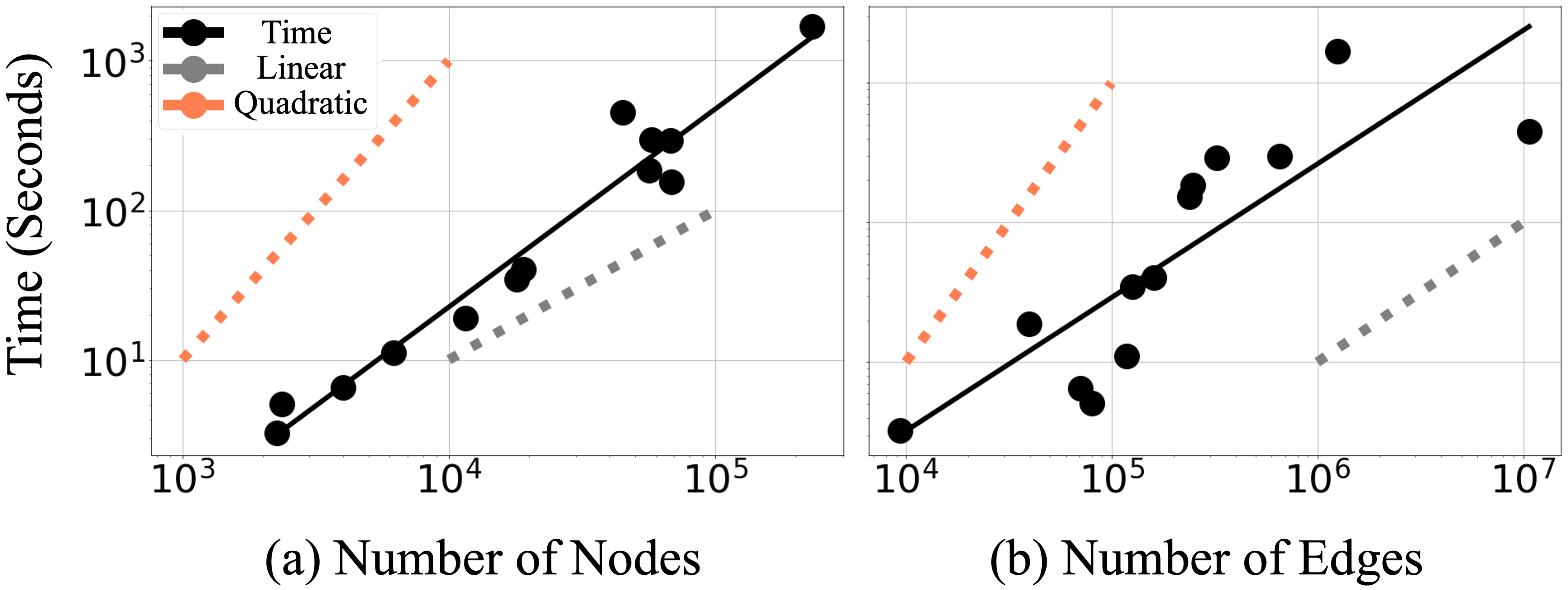
Figure 3: LinkWaldo is sub-quadratic on the number of nodes (a) and linear on the number of edges (b).

V-D Parameters (RQ3)

Setup. We evaluate the quality of different groupings (§ IV-A), and how the number of groups in each affects performance. On four graphs, Yeast, arXiv, Reddit, and Epinions, we run LinkWaldo with groupings DG, SG, and CG, varying the number of groups $|\Gamma|\in\{5,10,25,50,75,100\}$. We also investigate pairs of groupings, and the combination of all three groupings, via grid search of the number of groupings in each. We also evaluated $\tau\in\{1M,10M,25M,50M\}$, the tolerance for searching equivalence classes exactly vs. approximately with LSH, and $\zeta\in\{0,0.1,0.25,1/3,0.5,2/3\}$, the fraction of training pairs we allow the proximity function to miss before we bailout of an equivalence class.

Results. The results for the individual groupings are shown in Fig. 4. Grouping by log-binning nodes based on their degree, (i.e., DG) is in general the strongest grouping. Across all three groupings, we find that $|\Gamma|=25$ is a good number of groups. We found that using all three groupings was the best combination, with 25 log-bins, 5 structural clusters, and 5 communities (we omit the figures for brevity). For individual groupings, we observe diminishing returns, and in multiple groupings, slightly diminished performance when the number of groups in each grows large. We omit the figures for $\tau$ and $\zeta$, but found that $\tau=25M$ and $\zeta=0.5$ were the best parameters.

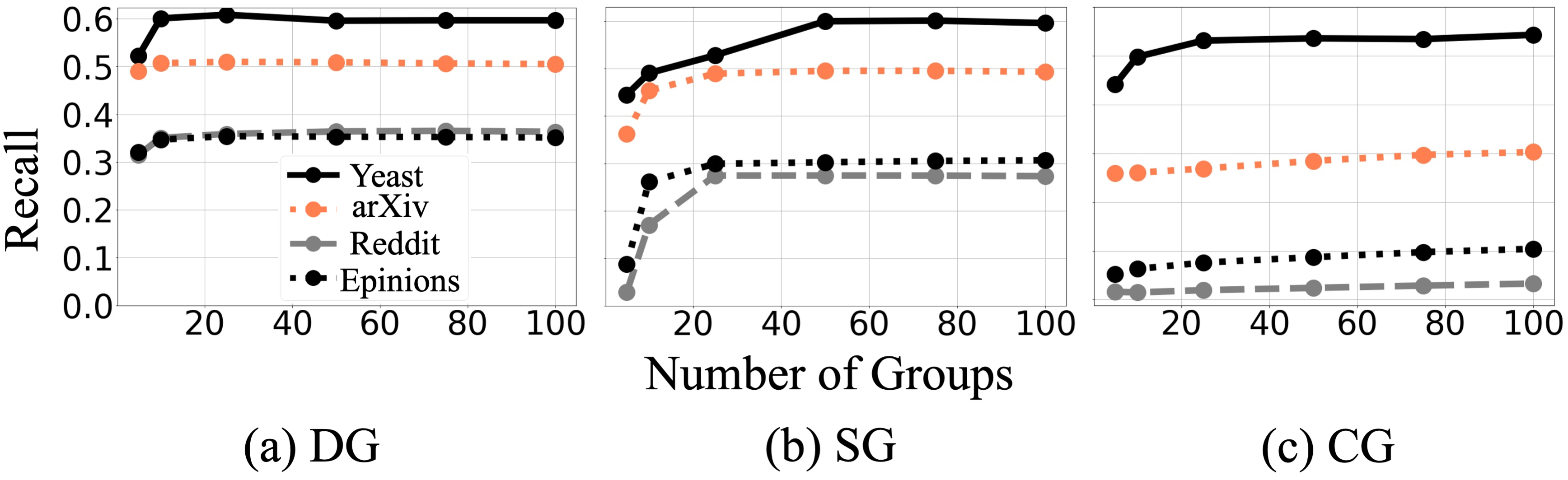
Figure 4: Number of groups for groupings DG, SG, and CG

VI Conclusion

In this paper, we focus on the under-studied and challenging problem of identifying a moderately-sized set of node pairs for a link prediction method to make decisions about. We mitigate the vastness of the search-space, filled with mostly non-links, by considering not just proximity, but also how much a pair of nodes resembles observed links. We formalize this idea in the Future Link Location Model, show its theoretical connections to stochastic block models and proximity models, and introduce an algorithm, LinkWaldo, that leverages it to return high-recall candidate sets, with only a tiny fraction of all pairs. Via our resemblance insight, LinkWaldo’s strong performance generalizes from social networks to protein networks. Future directions include investigating the directionality of links, since the roadmap can incorporate this information, and extending to heterogeneous graphs with many edge and node types, like knowledge graphs.

-A Effect of $k$

Table IV gives results (avgs over 3 seeds) for multiple values of $k$. For reasonable values of $k$—roughly up to an order of magnitude greater than $m$—results are mostly stable. The main exception is for small $k$, where NMF+Bag performs well in some cases. This is consistent with its design: to return a small, accurate set of top-$k$ predictions, rather than a candidate set.

Table IV: We report “$<k$” if fewer than $k$ pairs are returned. Black cells indicate values of $k$ outside the scale of the dataset.

	HS-Protein			Facebook2
Metric	NMF+Bag	AA	LinkWaldo-M	NMF+Bag	AA	LinkWaldo-M
R@10K	0.2629	0.1909	0.2251	0.0093	0.0103	0.0172
R@100K	$<k$	0.8443	0.9035	0.0422	0.0672	0.1106
R@1M	$<k$	0.9747	0.9847	0.0970	0.2832	0.3781
R@5M	N/A	N/A	N/A	$<k$	0.5561	0.5762

Table V: Input Proximity Model for LaPM and LinkWaldo, and parameter deviations from default for NMF+Bag.

Graph	LaPM	LinkWaldo-D	LinkWaldo-M	NMF+Bag
Yeast	NetMF-2	NetMF-2	NetMF-2	$\epsilon=0.5$
DBLP	NetMF-2	NetMF-2	NetMF-2	Default
Facebook1	NetMF-1	AA	AA	$\epsilon=0.1$
MovieLens	BiNE	BiNE	BiNE	$\epsilon=0.05$
HS-Protein	NetMF-2	NetMF-2	NetMF-2	$\epsilon=0.75$
arXiv	NetMF-2	AA	AA	Default
MathOverflow	NetMF-2	NetMF-1	NetMF-1	$\epsilon,\mu,f=0.5,0.3,0.3$
Enron	NetMF-2	NetMF-1	AA	Default
Reddit	NetMF-2	AA	AA	Default
Epinions	NetMF-1	AA	AA	Default
Facebook2	NetMF-2	AA	AA	Default
Digg	NetMF-2	NetMF-1	NetMF-1	Default
Protein-Soy	NetMF-1	NetMF-2	NetMF-2	Default

-B Complexity Analysis

Let $\gamma$ be the time complexity of the node grouping (S1). Computing the expected number of new edges in each cell (and variance), directly from the observed links, (S2) is $O(m)$. The complexity of searching equivalence classes (S3) comes from hashing each node in the decomposition $O(b_{\max})$ times, and finding the $\kappa_{i}$ closest pairs in the $O(\kappa_{i})$ pairs that land in the same bucket: $\sum_{\mathcal{C}_{i}\in\Pi}O(|\mathcal{V}_{u}\cup\mathcal{V}_{v}|b_{\max}+\kappa_{i})=O(nb_{\max}+k)$. This assumes that we do not encounter unrealistic scenarios, e.g., the embeddings being equivalent and hence inseparable, and that $b_{\max}$ is set large enough that the volume of tree leaves is not asymptotically larger than $O(\kappa_{i})$. Adding from the global pool (S4) takes $O(k)$ time, since $|\tilde{\mathcal{P}}_{G}|=O(k)$ and can be maintained in sorted order (similar to the merge in merge sort). Thus, the total time complexity is $O(\gamma+m+nb_{\max}+k)$.

References

- [1] Lada A Adamic and Eytan Adar. Friends and neighbors on the web. Social networks, 25(3):211–230, 2003.
- [2] Mayank Bawa, Tyson Condie, and Prasanna Ganesan. Lsh forest: self-tuning indexes for similarity search. In WWW, pages 651–660, 2005.
- [3] Caleb Belth, Xinyi Zheng, and Danai Koutra. Mining persistent activity in continually evolving networks. In KDD, 2020.
- [4] Moses S Charikar. Similarity estimation techniques from rounding algorithms. In STOC, 2002.
- [5] Liang Duan, Shuai Ma, Charu Aggarwal, Tiejun Ma, and Jinpeng Huai. An ensemble approach to link prediction. IEEE TKDE, 29(11), 2017.
- [6] Ming Gao, Leihui Chen, Xiangnan He, and Aoying Zhou. Bine: Bipartite network embedding. In SIGIR, 2018.
- [7] William L. Hamilton, Rex Ying, and Jure Leskovec. Representation learning on graphs: Methods and applications. IEEE Data Eng. Bull., 40(3):52–74, 2017.
- [8] Mark Heimann, Haoming Shen, Tara Safavi, and Danai Koutra. REGAL: Representation learning-based graph alignment. In CIKM, 2018.
- [9] Unmesh Joshi and Jacopo Urbani. Searching for embeddings in a haystack: Link prediction on knowledge graphs with subgraph pruning. In WebConf, 2020.
- [10] Thomas N Kipf and Max Welling. Variational graph auto-encoders. In NIPS Workshop on Bayesian Deep Learning, 2016.
- [11] Jérôme Kunegis. Konect: the koblenz network collection. In WWW, 2013.
- [12] Pierre Latouche, Etienne Birmelé, Christophe Ambroise, et al. Overlapping stochastic block models with application to the french political blogosphere. Annals App. Stat., 5(1):309–336, 2011.
- [13] Jure Leskovec and Andrej Krevl. SNAP Datasets: Stanford large network dataset collection. http://snap.stanford.edu/data, June 2014.
- [14] David A Levin and Yuval Peres. Markov chains and mixing times, volume 107. American Mathematical Soc., 2017.
- [15] David Liben-Nowell and Jon Kleinberg. The link-prediction problem for social networks. ASIS&T, 58(7):1019–1031, 2007.
- [16] Víctor Martínez, Fernando Berzal, and Juan-Carlos Cubero. A survey of link prediction in complex networks. CSUR, 49(4):1–33, 2016.
- [17] Nikhil Mehta, Lawrence Carin, and Piyush Rai. Stochastic blockmodels meet graph neural networks. In ICML, 2019.
- [18] Kurt Miller, Michael I Jordan, and Thomas L Griffiths. Nonparametric latent feature models for link prediction. In NeurIPS, 2009.
- [19] Mark EJ Newman. Mixing patterns in networks. Phys. Rev. E, 67(2), 2003.
- [20] Krzysztof Nowicki and Tom A B Snijders. Estimation and prediction for stochastic blockstructures. ASIS&T, 96(455):1077–1087, 2001.
- [21] Benjamin Pachev and Benjamin Webb. Fast link prediction for large networks using spectral embedding. J. Complex Netw., 6(1):79–94, 2018.
- [22] Jiezhong Qiu, Yuxiao Dong, Hao Ma, Jian Li, Kuansan Wang, and Jie Tang. Network embedding as matrix factorization: Unifying deepwalk, line, pte, and node2vec. In WSDM, pages 459–467, 2018.
- [23] Ryan Rossi and Nesreen Ahmed. The network data repository with interactive graph analytics and visualization. In AAAI, 2015.
- [24] Ryan A. Rossi, Di Jin, Sungchul Kim, Nesreen Ahmed, Danai Koutra, and John Boaz Lee. On proximity and structural role-based embeddings in networks: Misconceptions, techniques, and applications. TKDD, 2020.
- [25] Tara Safavi, Danai Koutra, and Edgar Meij. Evaluating the calibration of knowledge graph embeddings for trustworthy link prediction. In EMNLP, 2020.
- [26] Dongjin Song, David A Meyer, and Dacheng Tao. Top-k link recommendation in social networks. In ICDM, pages 389–398. IEEE, 2015.
- [27] Alexandre B Tsybakov. Introduction to nonparametric estimation. Springer Science & Business Media, 2008.
- [28] Jingdong Wang, Heng Tao Shen, Jingkuan Song, and Jianqiu Ji. Hashing for similarity search: A survey. arXiv preprint arXiv:1408.2927, 2014.
- [29] Muhan Zhang and Yixin Chen. Link prediction based on graph neural networks. In NeurIPS, pages 5165–5175, 2018.