Approximating viscosity solutions of the Euler system

Abstract

Applying the concept of S-convergence, based on averaging in the spirit of Strong Law of Large Numbers, the vanishing viscosity solutions of the Euler system are studied. We show how to efficiently compute a viscosity solution of the Euler system as the S-limit of numerical solutions obtained by the Viscosity Finite Volume method. Theoretical results are illustrated by numerical simulations of the Kelvin–Helmholtz instability problem.

^∗ Institute of Mathematics of the Czech Academy of Sciences

Žitná 25, CZ-115 67 Praha 1, Czech Republic

feireisl@math.cas.cz, she@math.cas.cz

^♣ Institute of Mathematics, TU Berlin

Strasse des 17. Juni, Berlin, Germany

^♠ Institute of Mathematics, Johannes Gutenberg-University Mainz

Staudingerweg 9, 55 128 Mainz, Germany

lukacova@uni-mainz.de, sschne15@uni-mainz.de

Keywords: barotropic Navier–Stokes system, isentropic Euler system, vanishing viscosity limit, viscosity finite volume method, oscillatory solution, Kolmogorov hypothesis

1 Introduction

The method of convex integration, adapted to problems in fluid mechanics by Buckmaster, De Lellis, Isett, Székelyhidi or Vicol [6, 12, 35] to name only a few, produced a large piece of evidence that the Euler system in fluid mechanics is ill posed, see also the survey paper [7] and the references cited therein. Another argument supporting ill–posedness of the incompressible Euler system was presented recently by Bressan and Murray [5]. Although one may still hope that the incompressible Euler system is well posed in the class of strong solutions, see however Elgindi and Jeong [18], this is definitely not the case if compressibility of the fluid is taken into account. Indeed Chiodaroli, De Lellis, and Kreml [10] provided an example of Lipschitz initial data for which the isentropic Euler system possesses infinitely many admissible weak solutions on a sufficiently long time lap. More recently, Chiodaroli et al. [11] identified even smooth ($C^{\infty}$) initial data yielding similar results.

As suggested by the numerical experiments of Elling [21], the “wild” solutions obtained through the abstract approach of convex integration may be physically relevant. The carbuncle solutions described in [21] departing for the initial data given by an admissible stationary state but being non–stationary may well represent a branch of energy dissipating “wild” solutions of the compressible Euler system predicted by convex integration.

In view of these facts, the Euler system being a model of perfect (ideal) fluid should be viewed in a broader context as an asymptotic limit of more complex systems describing real fluids including the effect of viscosity. Following the original idea of DiPerna and Majda [13, 14, 15] we identify a viscosity solution of the Euler system with a parametrized family of probability measures $\{\mathcal{V}_{t,x}\}_{t\in[0,T],x\in\Omega}$ generated by solutions of the Navier–Stokes system in the vanishing viscosity limit. Here $t$ is the time and $x$ the spatial coordinate in the domain $\Omega\subset\mathds{R}^{d}$ occupied by the fluid.

This process involves eventually approximation of the initial data for the Euler system. Here we should keep in mind that the vanishing viscosity limit may sensitively depend on the relation between the rate of convergence of the viscosity coefficients and the choice of the initial data approximation. As the Navier–Stokes system admits global in time weak solutions for any finite energy initial data relevant for the limit Euler system, this issue can be avoided by considering the same initial data for both systems. Another possibility is to focus on smooth initial data, for which the convergence is unconditional even for data perturbations at least on a short time interval. Both alternatives will be discussed below.

To separate the properties of $\mathcal{V}_{t,x}$ inherited from the generating sequence from those intrinsic to the limit Euler system, we identify a family of observables – functions of the state variables having the same expectation at any set of the physical space $(0,T)\times\Omega$ for all dissipative (viscosity) solutions $\mathcal{V}_{t,x}$, generated by the vanishing viscosity limit. There are several plausible scenarios of the vanishing viscosity limit:

• Oscillatory (weak) limit. The generating sequence of solutions of the viscous problem is merely bounded and converges weakly (in the sense of integral averages). The oscillations of the generating sequence can be described by a Young measure. In this case, the limit is not expected to be a weak solution of the Euler system, cf. [24].

• Statistical (strong) limit. There is a hidden regularizing effect acting in the vanishing viscosity limit so that the generating sequence is precompact in the strong $L^{p}-$topology. This phenomenon is intimately related to the celebrated Kolmogorov hypothesis advocated by Chen and Glimm [9] discussed in Section 6. The generating sequence is precompact but still may admit a non–trivial set of accumulation points. The convergence is understood in a statistical sense and may be described by a suitable measure sitting on the set of weak solutions of the Euler system.

• Unconditional (strong) limit. The generating sequence converges strongly to a single limit. In particular, this is the case when the limit Euler system admits a (unique) strong solution.

Of course, the vanishing viscosity limit may exhibit a mixture of the first and second alternative as the case may be. Our main goal is to propose a method how to approximate/compute efficiently the viscosity solutions, in particular the observable quantities in the case of oscillatory and/or statistical limit, that would be compatibly with the strong limit scenario as soon as it takes place. Note that, by virtue of the convergence result of Chen and Perepelitsa [8], the oscillatory scenario is excluded for problems in the spatial dimension $d=1$. On the other hand, oscillatory/statistical solutions are observed in numerical approximations of problems with unstable initial data, notably as perturbations of shock wave solutions, cf. Elling [19, 20] or emerging from the shear flow of the Kelvin–Helmholtz instability, cf. [28] or Fjordholm et al. [31, 32].

While a viscosity solution of the Euler system can be identified with a Young measure generated by a sequence of solutions of the Navier–Stokes system, its numerical approximation is calculated via the method of S–convergence proposed in [23]. Given a sequence of approximate (vanishing viscosity or numerical) solutions $\{{\bm{U}}_{n}\}_{n=1}^{\infty}$, we consider a family of probability measures

$$\mathcal{V}_{N}=\frac{1}{N}\sum_{n=1}^{N}\delta_{{\bm{U}}_{n}},\ \delta_{{\bm{U}}_{n}}-\mbox{the Dirac mass at}\ {\bm{U}}_{n},$$ (1.1)

or, alternatively, the associated family of parametrized probability measures

$$\left\{\mathcal{V}_{N}\right\}_{(t,x)\in(0,T)\times\Omega}=\frac{1}{N}\sum_{n=1}^{N}\delta_{{\bm{U}}_{n}(t,x)}.$$ (1.2)

Note carefully the subtle difference between (1.1) and (1.2). The measure $\mathcal{V}_{N}$ is a probability measure on the infinite dimensional space of trajectories – solutions of the approximate problem. The family $\left\{\mathcal{V}_{N}\right\}_{(t,x)\in(0,T)\times\Omega}$ consists of probability measures on the finite dimensional phase space – the range of the approximate solutions. In both cases, the limit for $N\to\infty$ fits in the framework of S–convergence developed in [23]. If suitable uniform bounds are available for $\{{\bm{U}}_{n}\}_{n=1}^{\infty}$, then the sequence $\{\mathcal{V}_{N}\}_{N=1}^{\infty}$ is tight and converges narrowly modulo a suitable subsequence to a limit $\mathcal{V}$ called S–limit. Here again, there is a conceptual difference between (1.1) and (1.2). The converging subsequence in (1.1) is obtained in terms of $N$ leaving the original sequence $\{{\bm{U}}_{n}\}_{n=1}^{\infty}$ unchanged, while in (1.2), the subsequence is selected from $\{{\bm{U}}_{n}\}_{n=1}^{\infty}$ in the spirit of Banach–Saks theorem.

The bulk of this paper is to study the asymptotic behavior of the parametrized measures (1.2). We consider a more general version,

$$\left\{\mathcal{V}_{N}\right\}_{(t,x)\in(0,T)\times\Omega}=\frac{1}{N}\sum_{n=1}^{N}s_{n,N}\delta_{{\bm{U}}_{n}(t,x)},$$ (1.3)

where $\{s_{n,N}\}$ is a suitable summation method. In contrast with the conventional Young measure obtained directly as a weak limit of the generating sequence, the S–limit in (1.2) is strong (a.a.) with respect to the independent variables $(t,x)$. This makes the limit object “visible” in numerical experiments. A similar construction based on the Cesàro averages ($s_{n,N}\equiv 1$) was used by Balder [1] to approximate conventional Young measures.

Our goal is to visualize – compute effectively the limit measure in (1.3). To this end, we propose a numerical method called viscosity finite volume (VFV) method of hybrid type that is not purely Euler oriented but involves the ghost effect of physical viscosity inherited from the sequence generating the viscosity solution. The original VFV method was introduced in [25, 29] and can be seen as a discretization (with vanishing viscosity) of the model proposed in a series of papers by Brenner [2, 3, 4], see also Guermond and Popov [33]. For the case of barotropic Euler system the method involves three vanishing, mutually interrelated parameters: the numerical step $h$, the shear viscosity coefficient $\mu$, and the bulk viscosity coefficient $\lambda$. We show that if $\mu=\mu(h)$, $\lambda=\lambda(h)$ are chosen such that

$$0<h<<\mu(h),\ \mu(h)\to 0,\lambda(h)\to 0\ \mbox{as}\ h\to 0,$$

then the VFV method produces a sequence of approximate solutions that admits an S–limit $\mathcal{V}$ that coincides with a viscosity solution of the Euler system. The latter will be precisely described in Definition 2.4. The corresponding limiting processes are depicted in the flow chart below. In particular, the observables are uniformly approximated in the strong topology of the Lebesgue space $L^{1}((0,T)\times\Omega)$.

The following are the main topics discussed in the present paper:

• In Section 2, we recall certain properties of the compressible (barotropic) Navier–Stokes system, in particular in the vanishing viscosity regime. Then we introduce the concept of viscosity solution to the Euler system.

• In Section 3, we revisit the theory of S–convergence introduced in [23] and discuss its relation to strong and weak convergence. We also show the subsequence principle claiming that any bounded sequence admits an S–convergent subsequence.

• In Section 4, we apply the abstract results to the barotropic Euler system. We identify the viscosity solutions with a Young measure generated in the vanishing viscosity limit of the Navier–Stokes problem. We also introduce the concept of generating sequence for a viscosity solution to be approximated later by a numerical scheme.

• In Section 5, we introduce the VFV method, discuss its structure preserving properties and show convergence to a viscosity solution of the Euler system. Theoretical results are illustrated by numerical experiments at the end of Section 5.

• Finally, the impact of Kolmogorov hypothesis is discussed in Section 6.

2 Euler and Navier–Stokes systems, viscosity solution

Consider a bounded regular domain $\Omega\subset\mathds{R}^{d}$, $d=2,3$ occupied by a fluid of a mass density $\varrho=\varrho(t,x)$ moving with the velocity ${\bm{u}}={\bm{u}}(t,x)$, where $x\in\Omega$ and $t\in[0,T]$ is the time. We suppose that the fluid is perfect and ignore thermal effects. Accordingly, the time evolution of the system is governed by the barotropic Euler system:

$$\begin{split}\partial_{t}\varrho+{\rm div}_{x}{\bm{m}}&=0,\ {\bm{m}}\equiv\varrho{\bm{u}},\\ \partial_{t}{\bm{m}}+{\rm div}_{x}\left(\frac{{\bm{m}}\otimes{\bm{m}}}{\varrho}\right)+\nabla_{x}p(\varrho)&=0,\end{split}$$ (2.1)

that may be supplemented with the impermeability boundary condition

$${\bm{m}}\cdot{\bm{n}}|_{\partial\Omega}=0,\ {\bm{n}}-\mbox{the outer normal vector.}$$ (2.2)

For the sake of simplicity, we focus on the isentropic pressure–density equation of state, $p(\varrho)\equiv a\varrho^{\gamma},\ a>0,\ \gamma>1$.

Real fluids are viscous, and, in accordance with the Second law of thermodynamics, they dissipate mechanical energy. Supposing the simplest linear (Newtonian) relation between the viscous stress and the symmetric velocity gradient, we consider the Navier–Stokes (NS) system:

$$\begin{split}\partial_{t}\varrho+{\rm div}_{x}(\varrho{\bm{u}})&=0,\\ \partial_{t}(\varrho{\bm{u}})+{\rm div}_{x}\left(\varrho{\bm{u}}\otimes{\bm{u}}\right)+\nabla_{x}p(\varrho)&={\rm div}_{x}\mathbb{S}(\nabla_{x}{\bm{u}}),\\ \mathbb{S}(\nabla_{x}{\bm{u}})&=\mu\left(\nabla_{x}{\bm{u}}+\nabla_{x}{\bm{u}}^{t}-\frac{2}{d}{\rm div}_{x}{\bm{u}}\mathbb{I}\right)+\lambda{\rm div}_{x}{\bm{u}}\mathbb{I},\ \mu>0,\ \lambda\geq 0.\end{split}$$ (2.3)

As mentioned above, our approach is based on identifying suitable solutions of the Euler system (2.1) as limits of (2.3) in the regime of vanishing viscosity coefficients $\mu$ and $\lambda$. As is well known, see e.g. the survey by E [16], this involves the problem of a boundary layer that may be created depending on the choice of the boundary conditions for the Navier–Stokes system, notably in the popular case of no–slip

$${\bm{u}}|_{\partial\Omega}=0.$$

To avoid this difficulty, the complete slip conditions

$${\bm{u}}\cdot{\bm{n}}|_{\partial\Omega}=0,\ [\mathbb{S}(\nabla_{x}{\bm{u}})\cdot{\bm{n}}]\times{\bm{n}}|_{\partial\Omega}=0$$ (2.4)

can be imposed. In view of future numerical implementation, we simplify even more by considering the space periodic boundary conditions for both the Euler and the Navier–Stokes system. In other words, we identify the spatial domain $\Omega$ with the flat torus,

$$\Omega\equiv{\mathcal{T}^{d}}=\left([0,1]|_{\{0,1\}}\right)^{d},\ d=2,3.$$ (2.5)

Note that the slip condition (2.4) can be equivalently reformulated in the periodic setting as soon as $\Omega$ is a cuboid, see Ebin [17].

2.1 Weak solutions to the Navier–Stokes system

The existence theory for the Navier–Stokes system (2.3) has been developed by Lions [37] and extended in [22] to accommodate a larger range of the adiabatic coefficient $\gamma>\frac{d}{2}$. The limit case $\gamma=1$, $d=2$ has been finally settled by Plotnikov and Weigant [39].

Definition 2.1 (Finite energy weak solution to NS system).

The functions $[\varrho,{\bm{u}}]$ are termed finite energy weak solution to the Navier–Stokes system (2.3) in $(0,T)\times{\mathcal{T}^{d}}$ with the initial conditions

$$\varrho(0,\cdot)=\varrho_{0},\ \varrho{\bm{u}}(0,\cdot)={\bm{m}}_{0}$$

if the following holds:

• Integrability

  $$\begin{split}\varrho&\in C_{\rm weak}([0,T];L^{\gamma}({\mathcal{T}^{d}})),\ \varrho\geq 0,\\ {\bm{u}}&\in L^{2}(0,T;W^{1,2}({\mathcal{T}^{d}};\mathds{R}^{d})),\ {\bm{m}}=\varrho{\bm{u}}\in C_{\rm weak}([0,T];L^{\frac{2\gamma}{\gamma+1}}({\mathcal{T}^{d}};\mathds{R}^{d})).\end{split}$$

• Equation of continuity

  $$\int_{0}^{T}\int_{{\mathcal{T}^{d}}}\Big{[}\varrho\partial_{t}\varphi+\varrho{\bm{u}}\cdot\nabla_{x}\varphi\Big{]}\ \,{\rm d}{x}\,{\rm d}t=-\int_{{\mathcal{T}^{d}}}\varrho_{0}\varphi\ \,{\rm d}{x}$$

  for any $\varphi\in C^{1}_{c}([0,T)\times{\mathcal{T}^{d}})$.

• Momentum equation

  $$\begin{split}\int_{0}^{T}\int_{{\mathcal{T}^{d}}}\Big{[}\varrho{\bm{u}}\cdot\partial_{t}\bm{\varphi}+\varrho{\bm{u}}\otimes{\bm{u}}:\nabla_{x}\bm{\varphi}+p(\varrho){\rm div}_{x}\bm{\varphi}\Big{]}\ \,{\rm d}{x}\,{\rm d}t&=\int_{0}^{T}\int_{{\mathcal{T}^{d}}}\mathbb{S}(\nabla_{x}{\bm{u}}):\nabla_{x}\bm{\varphi}\ \,{\rm d}{x}\,{\rm d}t\\ &-\int_{{\mathcal{T}^{d}}}{\bm{m}}_{0}\cdot\bm{\varphi}(0,\cdot)\ \,{\rm d}{x}\end{split}$$

  for any $\bm{\varphi}\in C^{1}_{c}([0,T)\times{\mathcal{T}^{d}};\mathds{R}^{d})$.

• Energy inequality

  $$\begin{split}\int_{{\mathcal{T}^{d}}}\Big{[}\frac{1}{2}\frac{|{\bm{m}}|^{2}}{\varrho}+\frac{a}{\gamma-1}\varrho^{\gamma}\Big{]}(\tau,\cdot)\ \,{\rm d}{x}&+\int_{0}^{\tau}\int_{{\mathcal{T}^{d}}}\mathbb{S}(\nabla_{x}{\bm{u}}):\nabla_{x}{\bm{u}}\ \,{\rm d}{x}\,{\rm d}t\\ &\leq\int_{{\mathcal{T}^{d}}}\Big{[}\frac{1}{2}\frac{|{\bm{m}}_{0}|^{2}}{\varrho_{0}}+\frac{a}{\gamma-1}\varrho_{0}^{\gamma}\Big{]}\ \,{\rm d}{x}\end{split}$$

  for any $0\leq\tau\leq T$.

The following result was proven in [22, Theorem 7.1].

Theorem 2.2 (Global existence for (NS) system).

Let $\gamma>\frac{d}{2}$ and let

$$\varrho_{0}\in L^{\gamma}({\mathcal{T}^{d}}),\ \varrho_{0}\geq 0,\ \int_{{\mathcal{T}^{d}}}\frac{|{\bm{m}}_{0}|^{2}}{\varrho_{0}}\ \,{\rm d}{x}<\infty.$$

Then the Navier–Stokes system admits a finite energy weak solution $[\varrho,{\bm{u}}]$ in $(0,T)\times{\mathcal{T}^{d}}$ in the sense of Definition 2.1 for any $T\leq\infty$.

2.2 Viscosity solutions to the Euler system

We are ready to introduce the concept of viscosity solution to the Euler system. We consider finite energy measurable initial data $[\varrho_{0},{\bm{m}}_{0}]$,

$$\varrho_{0}\geq 0,\ \int_{{\mathcal{T}^{d}}}\left[\frac{1}{2}\frac{|{\bm{m}}_{0}|^{2}}{\varrho_{0}}+\frac{a}{\gamma-1}\varrho_{0}^{\gamma}\right]\ \,{\rm d}{x}<\infty.$$

Definition 2.3 (Regular data approximation).

Let $[\varrho_{0},{\bm{m}}_{0}]$ be finite energy data. We say that a sequence $[\varrho_{0,n},{\bm{m}}_{0,n}]$ is a regular approximation of the data $[\varrho_{0},{\bm{m}}_{0}]$ if

$$\begin{split}\varrho_{0,n}\in W^{k,2}({\mathcal{T}^{d}}),\ {\bm{m}}_{0,n}&\in W^{k,2}({\mathcal{T}^{d}};\mathds{R}^{d})\ \mbox{for some}\ k\geq 3,\ \inf_{{\mathcal{T}^{d}}}\varrho_{0,n}>0,\\ \varrho_{0,n}&\to\varrho_{0}\ \mbox{weakly in}\ L^{1}({\mathcal{T}^{d}}),\ {\bm{m}}_{0,n}\to{\bm{m}}_{0}\ \mbox{weakly in}\ L^{1}({\mathcal{T}^{d}};\mathds{R}^{d}),\\ \int_{{\mathcal{T}^{d}}}\Big{[}\frac{1}{2}\frac{|{\bm{m}}_{0,n}|^{2}}{\varrho_{0,n}}+\frac{a}{\gamma-1}\varrho_{0,n}^{\gamma}\Big{]}\ \,{\rm d}{x}&\to\int_{{\mathcal{T}^{d}}}\Big{[}\frac{1}{2}\frac{|{\bm{m}}_{0}|^{2}}{\varrho_{0}}+\frac{a}{\gamma-1}\varrho_{0}^{\gamma}\Big{]}\ \,{\rm d}{x}.\end{split}$$

As is well–known, cf. e.g. Matsumura and Nishida [38] or Valli and Zajaczkowski [42], the Navier–Stokes system (2.3) admits a local in time classical solution for any initial data $[\varrho_{0,n},{\bm{m}}_{0,n}]$ in the regularity class specified in Definition 2.3.

Definition 2.4 (Viscosity solution of Euler system).

A parametrized family of probability measures

$$\mathcal{V}_{t,x}:(t,x)\in(0,T)\times{\mathcal{T}^{d}}\mapsto\mathfrak{P}({\mathds{R}}^{d+1}),\ \mathcal{V}\ \mbox{weakly measurable,}$$

where $\mathfrak{P}$ denotes the set of probability measures, is called viscosity solution of the Euler system (2.1) with the initial data $[\varrho_{0},{\bm{m}}_{0}]$ if there exists a regular approximation of the initial data $[\varrho_{0,n},{\bm{m}}_{0,n}]$, sequences of viscosity coefficients

$$\mu_{n}\searrow 0,\ \lambda_{n}\to 0,$$

and a sequence of finite energy weak solutions $[\varrho_{n},{\bm{m}}_{n}\equiv\varrho_{n}{\bm{u}}_{n}]_{n=1}^{\infty}$ of the Navier–Stokes system (2.3) starting from the initial data $[\varrho_{0,n},{\bm{m}}_{0,n}]$ such that

$$b(\varrho_{n},{\bm{m}}_{n})\to\overline{b(\varrho,{\bm{m}})}\ \mbox{weakly-(*) in}\ L^{\infty}((0,T)\times{\mathcal{T}^{d}})\ \mbox{for any}\ b\in C_{c}({\mathds{R}}^{d+1}),$$

where

$$\overline{b(\varrho,{\bm{m}})}(t,x)=\left<\mathcal{V}_{t,x};b(\tilde{\varrho},\tilde{{\bm{m}}})\right>\ \mbox{for a.a.}\ (t,x)\in(0,T)\times{\mathcal{T}^{d}}.$$

Thus a viscosity solution of the Euler system is simply a Young measure generated by a sequence of solutions of the Navier–Stokes system in the vanishing viscosity limit. The fact that the Navier–Stokes system admits a classical local in time solution for any regular approximation $[\varrho_{0,n},{\bm{m}}_{0,n}]$ of the initial data does not imply, of course, the existence of a “smooth” viscosity solution not even on a short time interval, as the life span of a potential generating sequence may shrink to zero for $n\to\infty$. However, in view of the existence result for the Navier–Stokes system stated in Theorem 2.2, a viscosity solution of the Euler system always exists at least if $\gamma>\frac{d}{2}$.

A viscosity solution may depend on the choice of (i) regular approximation of the initial data $[\varrho_{0,n},{\bm{m}}_{0,n}]_{n=1}^{\infty}$, (ii) the sequence of shear viscosity coefficients $\mu_{n}\searrow 0$, (iii) the sequence of bulk viscosity coefficients $\lambda_{n}\to 0$. To minimize the number of independent parameters we may omit the approximation of the initial data and consider directly $[\varrho_{0,n},{\bm{m}}_{0,n}]=[\varrho_{0},{\bm{m}}_{0}]$ as the Navier–Stokes admits global in time weak solutions for any finite energy data. Moreover, one can fix $\lambda$ as a function of $\mu$, in particular we may set $\lambda_{n}=0$, see Section 4.

As the vanishing viscosity limit is a consistent approximation of the Euler system in the sense of [25] (see [24]), any viscosity solution specified in Definition 2.4 is a dissipative measure valued (DMV) solution of the Euler system in the sense of [25].

Definition 2.5 (DMV solution of Euler system).

A parametrized family of probability measures

$$\mathcal{V}_{t,x}:(t,x)\in(0,T)\times{\mathcal{T}^{d}}\mapsto\mathfrak{P}({\mathds{R}}^{d+1}),\ \mathcal{V}\ \mbox{weakly measurable,}$$

is called dissipative measure valued (DMV) solution of the Euler system (2.1) with the initial conditions $[\varrho_{0},{\bm{m}}_{0}]$ if the following hold:

• Integrability

  $$\left<\mathcal{V};\tilde{\varrho}\right>\in C_{\rm weak}([0,T];L^{\gamma}({\mathcal{T}^{d}})),$$

  $$\left<\mathcal{V};\tilde{{\bm{m}}}\right>\in C_{\rm weak}([0,T];L^{\frac{2\gamma}{\gamma+1}}({\mathcal{T}^{d}};\mathds{R}^{d})).$$

• Equation of continuity

  $$\int_{0}^{T}\int_{{\mathcal{T}^{d}}}\Big{[}\left<\mathcal{V};\tilde{\varrho}\right>\partial_{t}\varphi+\left<\mathcal{V};\tilde{{\bm{m}}}\right>\cdot\nabla_{x}\varphi\Big{]}\ \,{\rm d}{x}\,{\rm d}t=-\int_{{\mathcal{T}^{d}}}\varrho_{0}\varphi(0,\cdot)\ \,{\rm d}{x}$$

  for any $\varphi\in C_{c}^{1}([0,T)\times{\mathcal{T}^{d}})$.

• Momentum equation

  $$\begin{split}&\int_{0}^{T}\int_{{\mathcal{T}^{d}}}\left[\left<\mathcal{V};\tilde{{\bm{m}}}\right>\cdot\partial_{t}\bm{\varphi}+\left<\mathcal{V};1_{\tilde{\varrho}>0}\frac{\tilde{{\bm{m}}}\otimes\tilde{{\bm{m}}}}{\tilde{\varrho}}\right>:\nabla_{x}\bm{\varphi}+\left<\mathcal{V};p(\tilde{\varrho})\right>{\rm div}_{x}\bm{\varphi}\right]\ \,{\rm d}{x}\,{\rm d}t\\ &=-\int_{{\mathcal{T}^{d}}}{\bm{m}}_{0}\cdot\bm{\varphi}\ \,{\rm d}{x}-\int_{0}^{T}\int_{{\mathcal{T}^{d}}}\nabla_{x}\bm{\varphi}:{\rm d}\mathfrak{R}(t)\,{\rm d}t\end{split}$$

  for any $\bm{\varphi}\in C^{1}_{c}([0,T)\times{\mathcal{T}^{d}};\mathds{R}^{d})$, with the Reynolds defect $\mathfrak{R}\in L^{\infty}(0,T;\mathcal{M}^{+}({\mathcal{T}^{d}};\mathds{R}^{d\times d}_{\rm{sym}}))$, where ${\mathcal{M}^{+}({\mathcal{T}^{d}};\mathds{R}^{d\times d}_{\rm{sym}})}$ denotes the space of positive semi-definite, symmetric matrix-valued measures.

• Energy inequality

  $$\int_{{\mathcal{T}^{d}}}\left<\mathcal{V}_{\tau,x};\frac{1}{2}\frac{|\tilde{{\bm{m}}}|^{2}}{\tilde{\varrho}}+P(\tilde{\varrho})\right>\ \,{\rm d}{x}+\int_{{\mathcal{T}^{d}}}{\rm d}\mathfrak{E}(\tau)\leq\int_{{\mathcal{T}^{d}}}\left[\frac{1}{2}\frac{|{\bm{m}}_{0}|^{2}}{\varrho_{0}}+P(\varrho_{0})\right]\ \,{\rm d}{x}$$

  holds for a.a. $0\leq\tau<T$, with the energy defect

  $$\mathfrak{E}\in L^{\infty}(0,T;\mathcal{M}^{+}({\mathcal{T}^{d}})).$$

• Defect compatibility

  $$\underline{d}\ \mathfrak{E}\leq{\rm tr}[\mathfrak{R}]\leq\overline{d}\ \mathfrak{E}\ \mbox{for some constants}\ 0<\underline{d}\leq\overline{d}.$$

DMV solutions represent the largest class of objects that can be identified as limits of consistent approximations of the Euler system. It is straightforward to show that any convex combination of DMV solutions is a DMV solution. In addition, the class of DMV solutions enjoys several remarkable properties, see [25], among which:

• Weak–strong uniqueness Suppose that the Euler system admits a Lipschitz solution $[\varrho,{\bm{m}}]$. Then

  $$\mathcal{V}_{t,x}=\delta_{\varrho(t,x),{\bm{m}}(t,x)}\ \mbox{for a.a.}\ (t,x)\in(0,T)\times{\mathcal{T}^{d}},\ \mathfrak{R}=\mathfrak{E}=0$$

  for any DMV solution emanating from the same initial data.

• Compatibility If

  $$(t,x)\mapsto\left<\mathcal{V}_{t,x};(\tilde{\varrho},\tilde{{\bm{m}}})\right>\in C^{1}([0,T]\times{\mathcal{T}^{d}};\mathds{R}^{d+1}),$$

  then

  $$\mathcal{V}_{t,x}=\delta_{\varrho(t,x),{\bm{m}}(t,x)}\ \mbox{for a.a.}\ (t,x)\in(0,T)\times{\mathcal{T}^{d}}$$

  where $[\varrho,{\bm{m}}]$ is a classical solution of the Euler system.

Being aware of the fact that the viscosity solution $\mathcal{V}$ may inherit certain features that depend on its generating sequence, we introduce the set of observables.

Definition 2.6 (Observables).

Let the initial data $[\varrho_{0},{\bm{m}}_{0}]$ be given. We say that a function $B\in C(\mathds{R}^{d+1})$ is observable for the Euler system if

$$\left<\mathcal{V}^{1}_{t,x};B(\widetilde{\varrho},\widetilde{{\bm{m}}})\right>=\left<\mathcal{V}^{2}_{t,x};B(\widetilde{\varrho},\widetilde{{\bm{m}}})\right>\ \mbox{a.a. in}\ (0,T)\times{\mathcal{T}^{d}}$$

whenever $\mathcal{V}^{1}$, $\mathcal{V}^{2}$ are viscosity solutions with the initial data $[\varrho_{0},{\bm{m}}_{0}]$.

Remark 2.7.

In general, the set of observables may also depend on the time $T$. In text below, we omit to mention explicitly this fact as $T$ is kept fixed.

Clearly, the set of all observables

$$\mathcal{O}[\varrho_{0},{\bm{m}}_{0}]=\left\{B\in C(\mathds{R}^{d})\ \Big{|}\ B\ \mbox{is observable for the Euler system with the data}\ [\varrho_{0},{\bm{m}}_{0}]\right\}$$

is a closed linear subspace of $C(\mathds{R}^{d})$ containing at least all constant functions. Moreover,

$$\mathcal{V}^{1}_{t,x}=\mathcal{V}^{2}_{t,x}\ \mbox{a.a. in}\ (0,T)\times{\mathcal{T}^{d}}\text{ for all viscosity solutions }\mathcal{V}^{1},\ \mathcal{V}^{2}\ \Leftrightarrow\ C_{c}(\mathds{R}^{d+1})\subset\mathcal{O}[\varrho_{0},{\bm{m}}_{0}].$$

The observables are quantities that are independent of the generating sequence and as such represent an intrinsic property shared by all viscosity solutions starting from the same initial data $[\varrho_{0},{\bm{m}}_{0}]$. In particular, the viscosity solution is unique if and only if all functions in $C_{c}(\mathds{R}^{d+1})$ are observables.

It is not excluded that the set of observables may depend on the initial data $[\varrho_{0},{\bm{m}}_{0}]$. Indeed, if the Euler system admits a $C^{1}$ solution, then $\mathcal{O}[\varrho_{0},{\bm{m}}_{0}]=C(\mathds{R}^{d+1})$, while it may not be the case if the barycenter of $\mathcal{V}$ is not smooth. It would be desirable though if at least the coordinates of the barycenter

$$\varrho=\left<\mathcal{V};\tilde{\varrho}\right>,\ {\bm{m}}=\left<\mathcal{V};\tilde{{\bm{m}}}\right>$$

were observables. In fact,

$${\bm{m}}=\left<\mathcal{V};\tilde{{\bm{m}}}\right>\ \mbox{observable}\ \Rightarrow\ \varrho=\left<\mathcal{V};\tilde{\varrho}\right>\ \mbox{observable},$$

which can be deduced from the fact that both quantities satisfy the continuity equation

$$\partial_{t}\left<\mathcal{V};\tilde{\varrho}\right>+{\rm div}_{x}\left<\mathcal{V};\tilde{{\bm{m}}}\right>=0$$

in the sense of distributions, with given initial data $\varrho_{0}$.

Our main goal in this paper is to show that a viscosity solution and, in particular, the observables can be effectively computed by means of a suitable numerical method.

2.3 Uniqueness of viscosity solutions

Given a sequence of solutions $[\varrho_{n},{\bm{m}}_{n}]_{n=1}^{\infty}$ to the Navier–Stokes system with the viscosity coefficients $\mu_{n}\searrow 0$, $\lambda_{n}\to 0$, emanating from a regularized approximation of the initial data $[\varrho_{0,n},{\bm{m}}_{0,n}]_{n=1}^{\infty}$, we may need a subsequence to generate a Young measure that represents a viscosity solution of the Euler system in the sense of Definition 2.4. If this is the case, the viscosity solution is obviously not unique. Although the numerical experiments performed and discussed in a series of papers by Elling [19, 20, 21] suggest this may be indeed possible, these results are based on approximating unstable initial data. In other words, the limit is sensitive to the choice of the approximate sequence $[\varrho_{0,n},{\bm{m}}_{0,n}]_{n=1}^{\infty}$. In view of these arguments, a more robust approximation of a viscosity solution will be introduced based on the concept of S–convergence discussed in the next section.

3 S–convergence and approximate solutions

The concept of S–convergence was introduced in [23]. The definition used in this paper is slightly different imposing more restrictions on the generating sequence.

3.1 S–convergence

An infinite matrix

$$\{s_{n,N}\}_{n=1,N=1}^{\infty}$$

is called regular summation method if the following properties are satisfied:

$$\begin{aligned} &\bullet\ \ 0\leq s_{n,N}\leq\overline{s}\ \mbox{for any}\ n,N,\mbox{ where }\overline{s}=\mbox{const.}\mbox{ independent of }n\mbox{ and }N,\\[5.69054pt] &\bullet\ \ s_{n,N}=0\ \mbox{whenever}\ n>N,\\ &\bullet\ \ \sum_{n=1}^{N}s_{n,N}=N\ \mbox{for any}\ N=1,2,\dots\end{aligned}$$ (3.1)

Remark 3.1.

Note that the first condition is usually replaced by a weaker stipulation

$$\sup_{n\leq N}\frac{s_{n,N}}{N}\to 0\ \mbox{as}\ N\to\infty$$

in the literature.

Definition 3.2 (S–convergence).

(i) Let

$${\bm{U}}_{n}:Q\subset\mathds{R}^{D}\to\mathds{R}^{m},D\mbox{ is an integer,}\ n=1,2,\dots$$

be a sequence of measurable (vector valued) functions. We say that $\{{\bm{U}}_{n}\}_{n=1}^{\infty}$ is S–convergent to a parameterized family of probability measures $\{\mathcal{V}_{y}\}_{y\in Q}$, $\mathcal{V}_{y}\in\mathfrak{P}(\mathds{R}^{m})$ for a.a. $y\in Q$,

$${\bm{U}}_{n}\stackrel{{\scriptstyle(S)}}{{\longrightarrow}}\mathcal{V}\ \mbox{with respect to a summation method}\ \{s_{n,N}\}$$

if

$$\int_{Q}w\left[\frac{1}{N}\sum_{n=1}^{N}s_{n,N}\delta_{{\bm{U}}_{n}(y)};\mathcal{V}_{y}\right]\ {\rm d}y\to 0\ \ \mbox{as}\ N\to\infty$$ (3.2)

where $w$ denotes the $1-$Wasserstein distance in $\mathfrak{P}(\mathds{R}^{m})$, cf. Villani [43].

(ii) We say that ${\bm{U}}_{n}$ is completely S–convergent to $\{\mathcal{V}_{y}\}_{y\in Q}$,

$${\bm{U}}_{n}\stackrel{{\scriptstyle(S)}}{{\Longrightarrow}}\mathcal{V},$$

if (3.2) holds for any regular summation method and any subsequence $\{{\bm{U}}_{n_{j}}\}_{j=1}^{\infty}$ of the original sequence.

Remark 3.3.

Note that convergence in (3.2) requires a uniform $L^{1}$-bound on the first moments of the family

$$\frac{1}{N}\sum_{n=1}^{N}s_{n,N}\delta_{{\bm{U}}_{n}(y)}.$$

In particular, the barycenter

$$\left<\mathcal{V};\widetilde{{\bm{U}}}\right>=\lim_{N\to\infty}\frac{1}{N}\sum_{n=1}^{N}s_{n,N}{\bm{U}}_{n}$$

is well–defined for a.a. $y\in Q$.

We proceed by stating a sufficient condition for a sequence of measurable vector valued functions to be S–convergent.

Lemma 3.4.

Let

$${\bm{U}}_{n}:Q\subset\mathds{R}^{D}\to\mathds{R}^{m},\ n=1,2,\dots$$

be a sequence of measurable (vector valued) functions defined on a bounded domain $Q\subset\mathds{R}^{D}$ that enjoys the following properties:

• $\{|{\bm{U}}_{n}|\}_{n=1}^{\infty}$ is equi–integrable in $Q$;

• For any $b\in C_{c}(\mathds{R}^{m})$ and a regular summation method ${\{s_{n,N}\}_{n=1,N=1}^{\infty}}$

  $$\frac{1}{N}\sum_{n=1}^{N}s_{n,N}b({\bm{U}}_{n})\to\overline{b({\bm{U}})}\ \mbox{in measure in}\ Q\ \mbox{as}\ N\to\infty.$$ (3.3)

  Then $\{{\bm{U}}_{n}\}_{n=1}^{\infty}$ is S–convergent with respect to ${\{s_{n,N}\}_{n=1,N=1}^{\infty}}$, and

  $${\bm{U}}_{n}\stackrel{{\scriptstyle(S)}}{{\longrightarrow}}\mathcal{V},\ \mbox{where}\ \left<\mathcal{V}_{y};b(\widetilde{{\bm{U}}})\right>=\overline{b({\bm{U}})}(y)\ \mbox{for a.a.}\ y\in Q.$$

Proof.

As $\{|{\bm{U}}_{n}|\}_{n=1}^{\infty}$ is equi–integrable we can by consider a sequence $b_{k}\in C_{c}(\mathds{R}^{m})$ with $b_{k}({\bm{U}})=b({\bm{U}})$ for $|{\bm{U}}|<k$ and $|b_{k}|<|b|$ to see that validity of (3.3) can be extended to any function

$$b\in C(\mathds{R}^{m}),\ |b({\bm{U}})|\lesssim 1+|{\bm{U}}|.$$

Next, we introduce a parametrized measure $\mathcal{V}$ as

$$\left<\mathcal{V}_{y},b(\widetilde{{\bm{U}}})\right>=\overline{b({\bm{U}})}(y)\ \mbox{for a.a.}\ y\in Q.$$

The convergence in (3.3) is equivalent to

$$d_{W^{*}}\left[\frac{1}{N}\sum_{n=1}^{N}s_{n,N}\delta_{{\bm{U}}_{n}(y)};\mathcal{V}_{y}\right]\to 0\ \mbox{in measure for}\ y\in Q,$$ (3.4)

where $d_{W^{*}}$ is the dual metric,

$$\begin{split}d_{W^{*}}[{\mathcal{V}_{1},\mathcal{V}_{2}}]&=\sum_{k=1}^{\infty}\frac{1}{2^{k}}\left|\left<{\mathcal{V}_{1}};b_{k}(\tilde{U})\right>-\left<{\mathcal{V}_{2}};b_{k}(\tilde{U})\right>\right|,\\ \{b_{k}\}_{k=1}^{\infty}&\subset C_{c}(\mathds{R}^{m})\ \mbox{a dense set in the unit ball in}\ C_{0}(\mathds{R}^{m}).\end{split}$$

Moreover, we also have convergence of the first moments,

$$\frac{1}{N}\sum_{n=1}^{N}s_{n,N}|{\bm{U}}_{n}(y)|\to\left<\mathcal{V}_{y};\widetilde{|{\bm{U}}|}\right>\ \mbox{in measure for}\ y\in Q.$$ (3.5)

As the sequence $\{{\bm{U}}_{n}\}_{n=1}^{\infty}$ is equi–integrable, the function

$$y\mapsto w\left[\frac{1}{N}\sum_{n=1}^{N}s_{n,N}\delta_{{\bm{U}}_{n}(y)};\mathcal{V}_{y}\right]$$

is equi–integrable as well. Consequently, to deduce the desired conclusion (3.2), it is enough to observe that

$$y\mapsto w\left[\frac{1}{N}\sum_{n=1}^{N}s_{n,N}\delta_{{\bm{U}}_{n}(y)};\mathcal{V}_{y}\right]\to 0\ \mbox{in measure for}\ y\in Q.$$

Assuming the contrary, we get $\varepsilon,\delta>0$ and a subsequence $N_{k}\to\infty$ such that

$$\left|y\in Q\ \Big{|}\ w\left[\frac{1}{N_{k}}\sum_{n=1}^{N_{k}}s_{n,N_{k}}\delta_{{\bm{U}}_{n}(y)};\mathcal{V}_{y}\right]>\varepsilon\right|>\delta\ \ \mbox{for }\ k\to\infty.$$ (3.6)

On the other hand, in accordance with (3.4), (3.5) and Villani [43, Theorem 6.9] , $\{N_{k}\}_{k=1}^{\infty}$ contains a subsequence (not relabeled) such that

$$w\left[\frac{1}{N_{k}}\sum_{n=1}^{N_{k}}s_{n,N_{k}}\delta_{{\bm{U}}_{n}(y)};\mathcal{V}_{y}\right]\to 0\ \mbox{as}\ k\to\infty\ \mbox{for a.a.}\ y\in Q$$

in contrast with (3.6).

∎

Next we focus on sufficient conditions that would guarantee (3.3). As the composition $b({\bm{U}}_{n})$ is bounded, it is enough to consider uniformly bounded sequences of measurable functions. We say that a set $\mathcal{S}\subset\mathds{N}\times\mathds{N}$ is statistically significant if

$$\frac{\#\{(n,m)\in\mathcal{S}\ \Big{|}\ n,m\leq N\}}{N^{2}}\to 1\ \ \mbox{as}\ N\to\infty.$$

Lemma 3.5.

Let $Q\subset\mathds{R}^{D}$ be a bounded domain and let

$${V}_{n}:Q\to\mathds{R},\ \|{V}_{n}\|_{L^{\infty}(Q)}\lesssim 1\ \mbox{uniformly for}\ n=1,2,\dots$$

be a bounded sequence of measurable functions. Suppose there exists $V\in L^{\infty}(Q)$ such that the set

$$\mathcal{S}(\varepsilon)=\left\{(n,m)\ \Big{|}\ s_{n,M}s_{m,M}\left|\int_{Q}(V_{n}-V)(V_{m}-V)\ {\rm d}y\right|<\varepsilon\;\mbox{ for all }M\in\mathds{N}\right\}$$

is statistically significant for any $\varepsilon>0$.

Then

$$\frac{1}{N}\sum_{n=1}^{N}s_{n,N}{V}_{n}\to V\ \mbox{in}\ L^{q}(Q)\ \mbox{as}\ N\to\infty,\ 1\leq q<\infty.$$ (3.7)

Proof.

As $\{V_{n}\}_{n=1}^{\infty}$ is uniformly bounded, it is enough to show

$$\frac{1}{N}\sum_{n=1}^{N}s_{n,N}{V}_{n}\to V\ \mbox{in}\ L^{2}(Q)$$

in other words

$$\int_{Q}\left|\frac{1}{N}\sum_{n=1}^{N}s_{n,N}(V_{n}-V)\right|^{2}\ {\rm d}y\to 0.$$

Denote

$$K_{N}(\varepsilon)=\left\{n,m\leq N\Big{|}\ s_{n,N}s_{m,N}\left|\int_{Q}(V_{n}-{V})(V_{m}-{V})\ {\rm d}y\right|\geq\varepsilon\right\}.$$

We have

$$\begin{split}&\int_{Q}\left|\frac{1}{N}\sum_{n=1}^{N}s_{n,N}(V_{n}-V)\right|^{2}\ {\rm d}y\leq\frac{1}{N^{2}}\sum_{n,m=1}^{N}s_{n,N}s_{m,N}\left|\int_{Q}(V_{n}-V)(V_{m}-V)\ {\rm d}y\right|\\ \\ &\leq\frac{1}{N^{2}}\sum_{n,m=1,(n,m)\in K_{N}(\varepsilon)}^{N}\overline{s}^{2}\left|\int_{Q}({V}_{n}-{V})({V}_{m}-{V})\ {\rm d}y\right|+\varepsilon\\ &\leq 4\overline{s}^{2}{|Q|\max\left\{\|V\|_{L^{\infty}(Q)},\ \sup_{n\geq 1}\|V_{n}\|_{L^{\infty}(Q)}\right\}^{2}}\frac{\#K_{N}(\varepsilon)}{N^{2}}+\varepsilon,\end{split}$$

where, in accordance with our hypothesis,

$$\frac{\#K_{N}(\varepsilon)}{N^{2}}\to 0\ \mbox{as}\ N\to\infty.$$

As $\varepsilon>0$ was arbitrary, the desired result follows. ∎

Corollary 3.6.

Let $Q\subset\mathds{R}^{D}$ be a bounded domain and let

$${V}_{n}:Q\to\mathds{R},\ \|{V}_{n}\|_{L^{\infty}(Q)}\lesssim 1\ \mbox{uniformly for}\ n=1,2,\dots$$

be a bounded sequence of measurable functions. Suppose there exists $V\in L^{\infty}(Q)$ such that the set

$$\mathcal{S}_{\varepsilon}=\left\{(n,m)\ \Big{|}\ \left|\int_{Q}(V_{n}-V)(V_{m}-V)\ {\rm d}y\right|<\varepsilon\right\}$$

is statistically significant for any $\varepsilon>0$.

Then

$$\frac{1}{N}\sum_{n=1}^{N}s_{n,N}{V}_{n}\to V\ \mbox{in}\ L^{q}(Q)\ \mbox{as}\ N\to\infty,\ 1\leq q<\infty.$$

for any regular summation method ${\{s_{n,N}\}_{n=1,N=1}^{\infty}}$.

3.2 Asymptotic stationarity

The disadvantage of Lemma 3.5 is that the sufficient condition for convergence depends on the a priori unknown limit $V$. To remove the problem we revisit the concept of asymptotic stationarity introduced in [23].

Proposition 3.7.

Let $Q\subset\mathds{R}^{D}$ be a bounded domain and let $\{V_{n}\}_{n=1}^{\infty}$ be a bounded sequence of measurable functions,

$$V_{n}\to V\ \mbox{weakly-(*) in}\ L^{\infty}(Q).$$

In addition, suppose that for any $\varepsilon>0$, $K\geq 1$, there exists $k=k(\varepsilon,K)\geq K$ such that

$$\begin{split}&\left\{(n,m)\Big{|}\ \left|\int_{Q}\Big{[}V_{n}V_{m}-V_{k+|n-m|}V_{k}\Big{]}\ {\rm d}y\right|<\varepsilon\right\}\\ &\mbox{is statistically significant.}\end{split}$$ (3.8)

Then

$$\frac{1}{N}\sum_{n=1}^{N}s_{n,N}{V}_{n}\to V\ \mbox{in}\ L^{q}(Q)\ \mbox{as}\ N\to\infty,\ 1\leq q<\infty$$

for any regular summation method $\{s_{n,N}\}_{n,N=1}^{\infty}$.

Proof.

First observe that it is enough to assume ${V}=0$. Indeed replacing ${V_{n}}\approx(V_{n}-V)$ we compute

$$\int_{Q}\Big{[}(V_{n}-V)(V_{m}-V)-(V_{k+|n-m|}-V)(V_{k}-V)\Big{]}\ {\rm d}y=\int_{Q}\Big{[}V_{n}V_{m}-V_{k+|n-m|}V_{k}\Big{]}\ {\rm d}y$$

$$+\int_{Q}V\Big{(}V_{k}+V_{k+|n-m|}-V_{m}-V_{n})\Big{)}\ {\rm d}y.$$ (3.9)

Next, by the weak-(*) convergence of $V_{n}$, we have the following property. For any $\varepsilon>0$ there exists $K=K(\varepsilon)\geq 1$, such that

$$\left|\int_{Q}V{\Big{(}V_{k}+V_{k+|n-m|}-V_{m}-V_{n}\Big{)}}\ {\rm d}y\right|<\frac{\varepsilon}{2}$$ (3.10)

whenever $m,n,k\geq K$. Now, hypothesis (3.8), together with (3.9), (3.10), imply that the set

$$\left\{(n,m)\Big{|}\ n,m\geq K,\left|\int_{Q}\Big{[}(V_{n}-V)(V_{m}-V)-(V_{k+|n-m|}-V)(V_{k}-V)\Big{]}\ {\rm d}y\right|<\frac{\varepsilon}{2}\right\}$$

is still statistically significant for $k=k\left(\frac{\varepsilon}{2},K\right)$; whence we may suppose $V\equiv 0$.

Now, fix $\varepsilon>0$ with the associated $k(\frac{\varepsilon}{2})$. It follows from hypothesis (3.8) that

$$\left\{(n,m)\Big{|}\ |n-m|\geq L,\left|\int_{Q}\Big{[}V_{n}V_{m}-V_{k+|n-m|}V_{k}\Big{]}\ {\rm d}y\right|<\frac{\varepsilon}{2}\right\}$$ (3.11)

is statistically significant for any $L\geq 1$. As $V_{n}\to 0$ weakly-(*) in $L^{\infty}(Q)$, we can fix $L$ so that

$$\left|\int_{Q}V_{k}V_{k+|n-m|}\ {\rm d}y\right|<\frac{\varepsilon}{2}\ \mbox{whenever}\ |n-m|\geq L.$$

Keep in mind that $k=k(\frac{\varepsilon}{2})$ is fixed at this stage.

Finally, it follows from (3.11) that

$$\left\{(n,m)\Big{|}\ \left|\int_{Q}V_{n}V_{m}\ {\rm d}y\right|<\varepsilon\right\}$$

is statistically significant for any $\varepsilon>0$ which, in view of Corollary 3.6, yields the desired conclusion.

∎

3.3 S–convergence vs. strong convergence

If

$${\bm{U}}_{n}\to{\bm{U}}\ \mbox{in}\ L^{1}(Q;\mathds{R}^{D}),$$

then it is easy to see, cf. [23, Corollary 3.4], that

$${\bm{U}}_{n}\stackrel{{\scriptstyle(S)}}{{\longrightarrow}}\delta_{{\bm{U}}}\ \mbox{for any regular summation method.}$$

Moreover, as the (strong) limit is unique, we get

$${\bm{U}}_{n}\stackrel{{\scriptstyle(S)}}{{\Longrightarrow}}\delta_{{\bm{U}}}.$$

A converse statement reads:

Lemma 3.8.

Let

$${\bm{U}}_{n}\to{\bm{U}}\ \mbox{weakly in}\ L^{1}(Q;\mathds{R}^{D}),$$

and

$$\frac{1}{N}\sum_{n=1}^{N}s_{n,N}b({\bm{U}}_{n})\to b({\bm{U}})\ \mbox{weakly-(*) in}\ L^{\infty}(Q)$$

for any $b\in C_{c}(\mathds{R}^{D})$ and some regular summation method $\{s_{n,N}\}$.

Then there is a subsequence $\{{\bm{U}}_{n_{j}}\}_{j=1}^{\infty}$ such that

$${\bm{U}}_{n_{j}}\to{\bm{U}}\ \mbox{in}\ L^{1}(Q;\mathds{R}^{D}).$$

Proof.

Given $b\in C_{c}(\mathds{R}^{D})$, we have

$$\frac{1}{N}\sum_{n=1}^{N}s_{n,N}b({\bm{U}}_{n})\to b({\bm{U}}),\ \frac{1}{N}\sum_{n=1}^{N}s_{n,N}{|b({\bm{U}}_{n})|^{2}}\to|b({\bm{U}})|^{2}\ \mbox{weakly-(*) in}\ L^{\infty}(Q),$$

in particular

$$\frac{1}{N}\sum_{n=1}^{N}s_{n,N}\int_{Q}|b({\bm{U}}_{n})-b({\bm{U}})|^{2}\ {\rm d}y\to 0\ \mbox{as}\ N\to\infty.$$

Consequently, there is a subsequence $n_{k}\to\infty$ such that

$$b({\bm{U}}_{n_{k}})\to b({\bm{U}})\ \mbox{in}\ L^{2}(Q).$$

Repeating the same argument for a family $\{b_{m}\}_{m=1}^{\infty}$ of functions $b$ dense in ${C_{c}(\mathds{R}^{D})}$ we obtain a subsequence $n_{j}$ such that

$$b({\bm{U}}_{n_{j}})\to b({\bm{U}})\ \mbox{in}\ L^{2}(Q)\ \mbox{for any}\ b\in C_{c}(\mathds{R}^{D}).$$

Due to the Dunford-Pettis theorem the sequence $\{{\bm{U}}_{n}\}_{n=1}^{\infty}$ is equi–integrable, which yields the desired conclusion.

∎

3.4 S–convergent subsequence principle

The following result was essentially proven by Balder [1] in the case of the Cesàro summation method $s_{n,N}=1$ for $n\leq N$. In contrast with [1], our approach is based on the Banach-Saks theorem, while [1] uses the Komlós theorem not available for arbitrary summation method.

Proposition 3.9 (Subsequence principle).

Let

$${\bm{U}}_{n}:Q\subset\mathds{R}^{D}\mapsto\mathds{R}^{m},\ Q\subset\mathds{R}^{D}\ \mbox{a bounded domain}$$

be an equi–integrable sequence of $L^{1}$ functions.

Then there are a subsequence $\{{\bm{U}}_{n_{j}}\}_{j=1}^{\infty}$ and a parametrized family of probability measures $\{\mathcal{V}_{y}\}_{y\in Q}\ \subset\mathfrak{P}(\mathds{R}^{m})$ such that

$${\bm{U}}_{n_{j}}\stackrel{{\scriptstyle(S)}}{{\Longrightarrow}}\mathcal{V}.$$

Proof.

Repeating the nowadays standard procedure leading to the construction of a Young measure we may extract a suitable subsequence (not relabeled) such that

$$b({\bm{U}}_{n})\to\overline{b({\bm{U}})}\ \mbox{weakly-(*) in}\ L^{\infty}(Q)\ \mbox{as}\ n\to\infty$$

for any $b\in C_{c}(\mathds{R}^{m})$. We set

$$\left<\mathcal{V}_{y},b(\tilde{U})\right>=\overline{b({\bm{U}})}(y)\ \mbox{for a.a.}\ y\in Q.$$

In accordance with Lemma 3.4, we have to show (3.3) for any regular method of summation. As $b$ is bounded, convergence in (3.3) is equivalent to

$$\frac{1}{N}\sum_{n=1}^{N}s_{n,N}b({\bm{U}}_{n})\to\overline{b({\bm{U}})}\ \mbox{in}\ L^{2}(Q)\ \mbox{as}\ N\to\infty$$ (3.12)

for any $b\in C_{c}(\mathds{R}^{m})$. The Hilbert space $L^{2}(Q)$ enjoys the Banach–Saks property. Specifically, any bounded sequence $\{v_{n}\}_{n=1}^{\infty}$ in $L^{2}(Q)$ contains a subsequence $\{v_{n_{j}}\}_{j=1}^{\infty}$ such that

$$\frac{1}{N}\sum_{j=1}^{N}v_{n_{j}}\to v\ \mbox{in}\ L^{2}(Q).$$

Thus, given $b\in C_{c}(\mathds{R}^{m})$, we may apply the alternative shown by Rosenthal [40] to conclude that there is a subsequence of indexes $\{n_{j}\}_{j=1}^{\infty}$ such that for any of its subsequences $\{n_{l}\}_{l=1}^{\infty}\subset\{n_{j}\}_{j=1}^{\infty}$ there holds

$$\frac{1}{N}\sum_{l=1}^{N}s_{{l},N}b({\bm{U}}_{n_{l}})\to\overline{b({\bm{U}})}\ \mbox{in}\ L^{2}(Q)$$

for any regular summation method $\{s_{n,N}\}$.

Repeating this argument successively for a family of functions $\{b_{m}\}_{m=1}^{\infty}$ dense in $C_{0}(\mathds{R}^{m})$ we obtain (3.12) for a suitable subsequence.

∎

4 Applications to the Euler system

We apply the abstract results obtained in Section 3 to the Euler system. We start by introducing the concept of generating sequence.

Definition 4.1 (Generating sequence).

Let $\mathcal{V}$ be a viscosity solution of the Euler system with the initial data $[\varrho_{0},{\bm{m}}_{0}]$.

We say that a sequence $[\varrho_{n},{\bm{m}}_{n}]_{n=1}^{\infty}$ of (weak) solutions to the Navier–Stokes system with $\mu_{n}\searrow 0$, $\lambda_{n}\to 0$ starting from regular approximation $[\varrho_{0,n},{\bm{m}}_{0,n}]_{n=1}^{\infty}$ is a generating sequence for $\mathcal{V}$ if

$$[\varrho_{n},{\bm{m}}_{n}]\stackrel{{\scriptstyle(S)}}{{\Longrightarrow}}\mathcal{V}.$$

4.1 Existence of viscosity solutions

The following result is a direct consequence of Theorem 2.2 on global existence for the Navier–Stokes system and the subsequence principle stated in Proposition 3.9.

Theorem 4.2 (Existence of viscosity solution).

Let $\gamma>\frac{d}{2}$ and let $[\varrho_{0},{\bm{m}}_{0}]$ be given finite energy initial data,

$$\varrho_{0}\geq 0,\ \int_{{\mathcal{T}^{d}}}\left[\frac{1}{2}\frac{|{\bm{m}_{0}}|^{2}}{\varrho_{0}}+\frac{a}{\gamma-1}\right]\ \,{\rm d}{x}<\infty.$$

Then

(i) the Euler system admits a viscosity solution $\{\mathcal{V}_{t,x}\}_{(t,x)\in(0,T)\times\Omega}$ in the sense of Definition 2.4;

(ii) there exists a regular approximation $[\varrho_{0,n},{\bm{m}}_{0,n}]$ of $[\varrho_{0},{\bm{m}}_{0}]$, and $\mu_{n}\searrow 0$, $\lambda_{n}\to 0$, such that the associated sequence of weak solutions $[\varrho_{n},{\bm{m}}_{n}]_{n=1}^{\infty}$ generates $\mathcal{V}$, specifically

$$[\varrho_{n},{\bm{m}}_{n}]\stackrel{{\scriptstyle(S)}}{{\Longrightarrow}}\mathcal{V}.$$

Proof.

It is a routine matter to construct a regular approximation $[\varrho_{0,n},{\bm{m}}_{0,n}]$ of the initial data $[\varrho_{0},{\bm{m}}_{0}]$ specified in Definition 2.3. Let $\mu_{n}\searrow 0$, $\lambda_{n}\to 0$ be a sequence of viscosity coefficients. Let $[\varrho_{n},{\bm{m}}_{n}=\varrho_{n}{\bm{u}}_{n}]_{n=1}^{\infty}$ be a sequence of finite energy weak solutions to the Navier–Stokes system with the initial data $[\varrho_{0,n},{\bm{m}}_{0,n}]$, the existence of which is guaranteed by Theorem 2.2.

As the energy

$$\int_{{\mathcal{T}^{d}}}\left[\frac{1}{2}\frac{|{\bm{m}}_{n}|^{2}}{\varrho_{n}}+\frac{a}{\gamma-1}\varrho_{n}^{\gamma}\right]\ \,{\rm d}{x}\ \mbox{is uniformly bounded for}\ t\in[0,T],$$

we deduce

$$\sup_{t\in[0,T]}\|\varrho_{n}(t,\cdot)\|_{L^{\gamma}({\mathcal{T}^{d}})}+\sup_{t\in[0,T]}\|{\bm{m}}_{n}(t,\cdot)\|_{L^{\frac{2\gamma}{\gamma+1}}({\mathcal{T}^{d}};\mathds{R}^{d}))}\leq c,$$

in particular $[\varrho_{n},{\bm{m}}_{n}]_{n=1}^{\infty}$ is equi–integrable in $(0,T)\times{\mathcal{T}^{d}}$. Consequently, by virtue of Proposition 3.9, there is a subsequence $[\varrho_{n_{j}},{\bm{m}}_{n_{j}}]_{j=1}^{\infty}$ generating the viscosity solution $\mathcal{V}$ in the sense of Definition 4.1.

∎

Of course, the existence result remains valid as long as the Navier–Stokes system admits a global–in–time finite energy weak solution for the given initial data. Due to the result of Plotnikov and Weigant [39], the existence still holds if $d=2$ and $\gamma\geq 1$. Similar extensions to a larger class of pressure–density state equations can be obtained via the existence theory developed in [22, Chapter 7].

4.2 Observables

We show that the observables - invariants of the class of viscosity solutions - can be identified with weak limits of solutions of the Navier–Stokes system.

Proposition 4.3 (Convergence of observables).

Let $B\in C(\mathds{R}^{d+1})$ satisfy

$$|B(\varrho,{\bm{m}})|\lesssim(1+\varrho+|{\bm{m}}|).$$

Then the following is equivalent:

• $B$ is observable in the sense of Definition 2.6 for the initial data $[\varrho_{0},{\bm{m}}_{0}]$;

• for any sequence of finite energy weak solutions $[\varrho_{n},{\bm{m}}_{n}]_{n=1}^{\infty}$ of the Navier–Stokes system with viscosity coefficients $\mu_{n}\searrow 0$, $\lambda_{n}\to 0$, starting from regular approximation $[\varrho_{0,n},{\bm{m}}_{0,n}]_{n=1}^{\infty}$ of the initial data $[\varrho_{0},{\bm{m}}_{0}]$, there holds

  $$B(\varrho_{n},{\bm{m}}_{n})\to\overline{B(\varrho,{\bm{m}})}\ \mbox{weakly in}\ {L^{r}((0,T)\times{\mathcal{T}^{d}})},\ r=\frac{2\gamma}{\gamma+1}.$$ (4.1)

Proof.

Suppose that $B\in\mathcal{O}[\varrho_{0},{\bm{m}}_{0}]$. As the energy of $[\varrho_{n},{\bm{m}}_{n}]_{n=1}^{\infty}$ is bounded, there is a subsequence such that

$$B(\varrho_{n_{j}},{\bm{m}}_{n_{j}})\to\mathcal{B}\ \mbox{weakly in}\ L^{r}((0,T)\times{\mathcal{T}^{d}}),\ r=\frac{2\gamma}{\gamma+1}\leq\gamma.$$ (4.2)

By virtue of the subsequence principle stated in Proposition 3.9, there is yet another subsequence $\{n_{l}\}_{l=1}^{\infty}\subset\{n_{j}\}_{j=1}^{\infty}$ such that

$$[\varrho_{n_{l}},{\bm{m}}_{n_{l}}]{\stackrel{{\scriptstyle(S)}}{{\Longrightarrow}}}\mathcal{V},$$

where $\mathcal{V}$ is a viscosity solution of the Euler system with the initial data $[\varrho_{0},{\bm{m}}_{0}]$. Since $B$ is observable, convergence in (3.2) yields

$$\mathcal{B}=\left<\mathcal{V};B(\tilde{\varrho},\tilde{{\bm{m}}})\right>\equiv\overline{B(\varrho,{\bm{m}})}.$$

As the same argument can be applied to any subsequence satisfying (4.2) we get unconditional convergence claimed (4.1).

The opposite implication can be shown by the same argument yielding a unique value

$$\left<\mathcal{V};B(\tilde{\varrho},\tilde{{\bm{m}}})\right>=\overline{B(\varrho,{\bm{m}})}$$

for any viscosity solution $\mathcal{V}$, meaning $B\in\mathcal{O}[\varrho_{0},{\bm{m}}_{0}]$.

∎

Thus the value of observables is uniquely determined as the weak limit of their composition with arbitrary generating sequence. In particular, any such sequence generates a (unique) Young measure $\mathcal{V}$ if $C_{c}(R^{d+1})\subset\mathcal{O}[\varrho_{0},{\bm{m}}_{0}]$. If this is the case, the measure $\mathcal{V}$ is the unique viscosity solution of the Euler system.

5 Numerical method – approximate solutions

As shown in the preceding section, observables are independent of the particular choice of the vanishing viscosity coefficients $\mu_{n}$, $\lambda_{n}$ and the approximation of the initial data $(\varrho_{0,n},{\bm{m}}_{0,n})$ and as such reflect intrinsic properties of the limit Euler system. Our principal objective is to show how to compute the observables by means of a suitable numerical scheme. We distinguish three basic parameters characterizing the approximation process: the numerical step $h$, typically a mesh size, the artificial viscosity coefficients $\mu$ and $\lambda$. In view of various restrictions imposed in particular by the consistency estimates, we focus on parameters $(h,\mu,\lambda)$ ranging in a set $\mathcal{R}$,

$$[h,\mu,\lambda]\in\mathcal{R}\subset(0,1]\times(0,1]\times[0,1],\ (0,0,0)\in\overline{\mathcal{R}}.$$

Typically,

$$\mathcal{R}=\left\{[h,\mu,\lambda]\ \Big{|}\ 0<h^{\alpha}<c\mu;\mbox{ either }\lambda=0\mbox{ or }0<h^{\alpha}\leq c\lambda\right\}\ \mbox{for some}\ \alpha>0.$$ (5.1)

The region $\mathcal{R}$ is determined by the range of parameters for which a particular numerical method converges, cf. Theorem 5.2 below. In general, we consider the situation where the numerical step $h$ is largely dominated by the (artificial) viscosity, $h<<\min(\mu,\lambda)$ if $\mu,\lambda>0$. This is in line with our philosophy that the problem should be close to the generating sequence of the Navier–Stokes solutions with low viscosity.

In what follows we introduce a particular numerical method, the so-called vanishing viscosity finite volume method. It is based on the model proposed in [3, 4] by H. Brenner as an alternative to the conventional Navier–Stokes system, see also [29].

5.1 Viscosity Finite Volume (VFV) method

We start by introducing a discretization of the computational domain and the discrete differential operators. The physical domain $\Omega\equiv\mathcal{T}^{d}$, $d=2,3$, is decomposed into compact elements,

$$\mathcal{T}^{d}=\bigcup_{K\in\mathcal{T}_{h}}K.$$

The elements $K$ are chosen to be rectangular/cuboid. The mesh $\mathcal{T}_{h}$ satisfies standard regularity properties. The set of all faces $\sigma\in\partial K,$ $K\in\mathcal{T}_{h}$ is denoted by $\Sigma.$ We suppose $|K|\approx h^{d},\ |\sigma|\approx h^{d-1}\ \mbox{ for any }\ K\in\mathcal{T}_{h},\mbox{ and }\sigma\in\Sigma,$ where the parameter $h\in(0,1)$ denotes the size of the mesh $\mathcal{T}_{h}.$

We denote ${Q}_{h}$ the space of functions that are constant on each element $K\in\mathcal{T}_{h}$, with the associated projection:

$$\Pi_{h}:L^{1}(\mathcal{T}^{d})\to{Q}_{h},\ \Pi_{h}v=\sum_{K\in\mathcal{T}_{h}}1_{K}\frac{1}{|K|}\int_{K}v\,{\rm d}{x}.$$

For the average and jump of $v\in Q_{h}$ on a face $\sigma\in\Sigma$ we have the following discrete operators, respectively,

$$\left\{\!\!\left\{v\right\}\!\!\right\}(x)=\frac{v^{\rm in}(x)+v^{\rm out}(x)}{2},\ \ \ \left[\!\left[v\right]\!\right]=v^{\rm out}(x)-v^{\rm in}(x).$$

Here $v^{\rm out},v^{\rm in}$ are respectively the outward, inward limits with respect to a given normal ${\bm{n}}$ belonging to $\sigma\in\Sigma.$ We define the following discrete differential operators for piecewise constant functions $r_{h}\in Q_{h},$ $\bm{v}_{h}\in{\bm{Q}}_{h}\equiv Q_{h}^{d}$:

$$\nabla_{h}r_{h}=\sum_{K\in\mathcal{T}_{h}}(\nabla_{h}r_{h})_{K}1_{K},\quad(\nabla_{h}r_{h})_{K}=\sum_{\sigma\in\partial K}\frac{|\sigma|}{|K|}\left\{\!\!\left\{r_{h}\right\}\!\!\right\}{\bm{n}},$$

$$\Delta_{h}r_{h}=\sum_{K\in\mathcal{T}_{h}}(\Delta_{h}r_{h})_{K}1_{K},\quad(\Delta_{h}r_{h})_{K}=\sum_{\sigma\in\partial K}\frac{|\sigma|}{|K|}\frac{\left[\!\left[r_{h}\right]\!\right]}{h},$$

$$\nabla_{\mathcal{D}}r_{h}=\sum_{\sigma\in\partial K}\left(\nabla_{\mathcal{D}}r_{h}\right)_{\sigma}1_{\sigma},\quad\left(\nabla_{\mathcal{D}}r_{h}\right)_{\sigma}=\frac{\left[\!\left[r_{h}\right]\!\right]}{h}{\bm{n}}$$

$${\rm div}_{h}\bm{v}_{h}=\sum_{K\in\mathcal{T}_{h}}({\rm div}_{h}\bm{v}_{h})_{K}1_{K},\quad({\rm div}_{h}\bm{v}_{h})_{K}=\sum_{\sigma\in\partial K}\frac{|\sigma|}{|K|}\left\{\!\!\left\{\bm{v}_{h}\right\}\!\!\right\}\cdot{\bm{n}}$$

$${\rm div}_{h}^{{\rm up}}(r_{h},\bm{v}_{h})=\sum_{K\in\mathcal{T}_{h}}1_{K}{\rm div}_{h}^{{\rm up}}(r_{h},\bm{v}_{h})_{K},\quad{\rm div}_{h}^{{\rm up}}(r_{h},\bm{v}_{h})_{K}=\sum_{\sigma\in\partial K}\frac{|\sigma|}{|K|}F_{h}(r_{h},\bm{v}_{h}).$$

Here $F_{h}$ denotes the classical upwind flux ${\mbox{\sl{Up}}}[r_{h},\bm{v}_{h}]$ with an additional numerical diffusion, specifically

$$\mbox{\sl{Up}}[r_{h},{\bm{v}}_{h}] = \left\{\!\!\left\{r_{h}\right\}\!\!\right\}\ \left\{\!\!\left\{{\bm{v}}_{h}\right\}\!\!\right\}\cdot{\bm{n}}-\frac{1}{2}|\left\{\!\!\left\{{\bm{v}}_{h}\right\}\!\!\right\}\cdot{\bm{n}}|\left[\!\left[r_{h}\right]\!\right]$$

$$F_{h}(r_{h},\bm{v}_{h}) = {\mbox{\sl{Up}}}[r_{h},\bm{v}_{h}]-h^{\varepsilon}\left[\!\left[r_{h}\right]\!\right]=\left\{\!\!\left\{r_{h}\right\}\!\!\right\}\ \left\{\!\!\left\{{\bm{v}}_{h}\right\}\!\!\right\}\cdot{\bm{n}}-\left(h^{\varepsilon}+\frac{1}{2}|\left\{\!\!\left\{{\bm{v}}_{h}\right\}\!\!\right\}\cdot{\bm{n}}|\right)\left[\!\left[r_{h}\right]\!\right],\ -1<\varepsilon.$$

Moreover, we denote ${\bf F}_{h}({\bf r}_{h},\bm{v}_{h})=(F_{h}(r_{1,h},\bm{v}_{h}),\cdots,F_{h}(r_{d,h},\bm{v}_{h}))^{T}$ for ${\bf r}_{h}=(r_{1,h},\cdots,r_{d,h})^{T}$.

In order to discretize the time evolution in $[0,T]$ we introduce a time step $\Delta t>0,$ $\Delta t\approx h,$ and denote

$$t_{k}=k\Delta t,\ k=1,2,\dots,N_{T}.$$

Furthermore,

$$v^{k}(x)=v(t^{k},x)\ \mbox{ for all }\ x\in\Omega,\ t^{k}=k\,\Delta t\ \mbox{ for }k=0,1,\ldots,N_{T}.$$

The time derivative $\frac{\partial{v}}{\partial t}$ is approximated by the backward Euler finite difference

$$\frac{\partial{v}}{\partial t}\Big{|}_{t^{k}}\approx D_{t}{v}^{k}\equiv\frac{{v}^{k}-{v}^{k-1}}{\Delta t}.$$

Finally, we introduce a piecewise constant interpolation in time of the discrete values $v^{k}$,

$$v_{h}(t,\cdot)=v_{0}\mbox{ for }t<\Delta t,\ v_{h}(t,\cdot)=v^{k}\mbox{ for }t\in[k\Delta t,(k+1)\Delta t),\ k=1,2,\ldots,N_{T}.$$ (5.2)

Let $(\varrho_{h}^{0},{\bm{u}}_{h}^{0})=(\Pi_{h}\varrho_{0},\Pi_{h}{\bm{u}}_{0})\in Q_{h}\times{\bm{Q}}_{h},$ ${\bm{m}}_{h}^{0}\equiv\varrho_{h}^{0}{\bm{u}}_{h}^{0}$ be the discrete initial data.

Definition 5.1 (VFV numerical scheme).

A pair $(\varrho_{h},{\bm{m}}_{h}\equiv\varrho_{h}{\bm{u}}_{h})$ of piecewise constant functions (in space and time) is a numerical approximation of the Euler system (2.1) by viscosity finite volume (VFV) method if the following system of discrete equations holds:

$$D_{t}\varrho_{h}+{\rm div}_{h}^{{\rm up}}(\varrho_{h},{\bm{u}}_{h}) = 0,$$

$$D_{t}(\varrho_{h}{\bm{u}}_{h})+{\rm div}_{h}^{{\rm up}}(\varrho_{h}{\bm{u}}_{h},{\bm{u}}_{h})+\nabla_{h}p_{h} = \mu(h)\Delta_{h}{\bm{u}}_{h}+\nu(h)\nabla_{h}{\rm div}_{h}{\bm{u}}_{h},$$ (5.3)

where $\nu(h)=\frac{1}{3}\mu(h)+\lambda(h)$ and the discrete pressure is $p_{h}=a\varrho_{h}^{\gamma}.$

It is convenient to rewrite (5.3) in the weak form

$$\int_{{\mathcal{T}^{d}}}D_{t}\varrho_{h}\varphi_{h}\ \,{\rm d}{x}-\sum_{\sigma\in\mathcal{E}}\int_{\sigma}F_{h}(\varrho_{h},{\bm{u}}_{h})\left[\!\left[\varphi_{h}\right]\!\right]\,\mathrm{d}S_{x}=0\quad\mbox{for all }\varphi_{h}\in{Q}_{h},$$ (5.4a)

$$\int_{{\mathcal{T}^{d}}}D_{t}(\varrho_{h}{\bm{u}}_{h})\cdot\bm{\varphi}_{h}\ \,{\rm d}{x}-\sum_{\sigma\in\mathcal{E}}\int_{\sigma}{\bf F}_{h}(\varrho_{h}{\bm{u}}_{h},{\bm{u}}_{h})\cdot\left[\!\left[\bm{\varphi}_{h}\right]\!\right]\,\mathrm{d}S_{x}-\sum_{\sigma\in\mathcal{E}}\int_{\sigma}\left\{\!\!\left\{p(\varrho_{h})\right\}\!\!\right\}{\bm{n}}\cdot\left[\!\left[\bm{\varphi}_{h}\right]\!\right]\,\mathrm{d}S_{x}$$

$$=-\mu(h)\frac{1}{h}\sum_{\sigma\in\mathcal{E}}\int_{\sigma}\left[\!\left[{\bm{u}}_{h}\right]\!\right]\cdot\left[\!\left[\bm{\varphi}_{h}\right]\!\right]\,\mathrm{d}S_{x}-\nu(h)\int_{{\mathcal{T}^{d}}}{\rm div}_{h}{\bm{u}}_{h}{\rm div}_{h}\bm{\varphi}_{h}\ \,{\rm d}{x},\quad\mbox{for all }\bm{\varphi}_{h}\in{\bm{Q}}_{h}.$$ (5.4b)

Note that the VFV method (5.3) or (5.4) mimics the physical process of vanishing viscosity limit in the Navier–Stokes system discussed in Section 4. In particular, we expect to recover the observables as limits of the numerical solutions as long as the numerical step $h$ is largely dominated by the (vanishing) viscosity coefficients.

5.2 Structure preserving properties and convergence of VFV method

We recall some fundamental properties of the VFV method shown in [27, 29].

• Conservation of discrete mass
  

  $$\int_{{\mathcal{T}^{d}}}\varrho_{h}(t,\cdot)\ \,{\rm d}{x}=\int_{{\mathcal{T}^{d}}}\varrho_{0,h}\ \,{\rm d}{x}=M_{0}>0,\,\ t\geq 0.$$

• Positivity of the discrete density
  

  $$\varrho_{h}(t)>0\ \mbox{ for any }t>0\mbox{ provided }\varrho_{h}(0)>0.$$

• Discrete total energy dissipation
  

  $$D_{t}\int_{{\mathcal{T}^{d}}}\left(\frac{1}{2}\varrho_{h}|{\bm{u}}_{h}|^{2}+\frac{(\varrho_{h})^{\gamma}}{\gamma-1}\right)\,\,{\rm d}{x}+\mu(h)\left\lVert\nabla_{\mathcal{D}}{\bm{u}}_{h}\right\rVert_{L^{2}}^{2}+\nu(h)\left\lVert{\rm div}_{h}{\bm{u}}_{h}\right\rVert_{L^{2}}^{2}\leq 0.$$

In [25, 29], we have established the following convergence result for the VFV method, see also [26] for further details.

Theorem 5.2 (Weak convergence of VFV method/Euler limit).

Let $\{\varrho_{h},{\bm{m}}_{h}\}_{h\searrow 0}$ be a family of solutions generated by the VFV method (5.3) with $\Delta t\approx h$. Let the initial data satisfy

$$\varrho_{0}\in L^{\infty}(\Omega),\ {\bm{m}}_{0}\in L^{\infty}(\Omega),\qquad\varrho_{0}>0.$$

Further, we suppose that $\mu(h)\geq h^{\alpha},$ $\nu(h)\geq h^{\alpha}$, and $\mu(h)\to 0$, $\nu(h)\to 0,$ cf. (5.1),

$$\begin{split}&-1<\varepsilon\mbox{ and }\ 0<\alpha<2-\frac{d/3+1+\varepsilon}{\gamma}\quad\mbox{ for }\gamma\in(1,2),\\ \mbox{or}\quad&-1<\varepsilon\ \mbox{ and }\ 0<\alpha<2-\frac{d}{\gamma}\quad\mbox{ for }\gamma\geq 2.\\ \end{split}$$ (5.5)

Then at least for a subsequence the numerical solutions $\{\varrho_{h},{\bm{m}}_{h}\}_{h\searrow 0}$ of the VFV method (5.3) give rise to a Young measure $\{{\mathcal{V}_{t,x}}\}_{(t,x)\in(0,T)\times\Omega}$ that represents a dissipative measure valued solution of the Euler system (2.1) in the sense of Definition 2.5.

As suggested by Elling [21] the viscosity solution may depend on the relation between the viscosity coefficients $\mu,\,\lambda$. To avoid this ambiguity we consider the specific case $\lambda=0,$ meaning $\nu=\frac{1}{3}\mu.$ Note that this corresponds to the Stokes hypothesis for gases.

The VFV method is of hybrid type. On the one hand, it yields a solution to the Euler system provided the viscosity coefficients go to zero along with the numerical step as in (5.5). On the other hand, it is a converging numerical approximation of the Navier–Stokes system (2.1) as long as we set the viscosity coefficients $\mu(h)=\rm{const.},$ $\nu(h)=\rm{const.}$ Indeed, as shown in [27],

$$\begin{split}\varrho_{h}&\rightarrow\varrho\mbox{ (strongly) in }L^{1}(0,T)\times{\mathcal{T}^{d}}),\\ {\bm{u}}_{h}&\rightarrow{\bm{u}}\mbox{ (strongly) in }L^{1}((0,T)\times{\mathcal{T}^{d}};\mathds{R}^{d}),\end{split}$$ (5.6)

as soon as the Navier–Stokes system admits a strong solution $(\varrho,{\bm{u}})$ on $(0,T)\times{\mathcal{T}^{d}}.$

In particular, there exists $\overline{\varrho}$ such that

$$\left|\left\{\varrho_{h}\geq\overline{\varrho}\right\}\right|\to 0\qquad h\searrow 0,$$

where $|\cdot|$ denotes the Lebesque measure on $(0,T)\times{\mathcal{T}^{d}}.$ As $\varrho_{h}$ is constant on each element, this is equivalent to

$$\#\left\{K\times[t_{i},t_{i+1});K\in\mathcal{T}_{h},i=1\dots N_{T}\Big{|}\varrho_{h}\geq\overline{\varrho}\right\}h^{d+1}\to 0\mbox{ for }h\searrow 0.$$

Interestingly, this condition is also sufficient for the convergence claimed in (5.6).

Theorem 5.3 (Strong convergence of VFV method/Navier–Stokes limit).

Suppose $\mu(h)={\rm{const.}}$, $\lambda(h)=\nu(h)-\frac{1}{3}\mu(h)=0.$ Let the initial data belong to the class

$$\varrho_{0}\in W^{3,2}({\mathcal{T}^{d}}),\ \varrho_{0}>0,\ {\bm{m}}_{0}=\varrho_{0}{\bm{u}}_{0},\ {\bm{u}}_{0}\in W^{3,2}({\mathcal{T}^{d}};\mathds{R}^{d}).$$ (5.7)

Let $\{\varrho_{h},{\bm{u}}_{h}\}_{h\searrow 0}$ be a family of solutions of the VFV method (5.3).

Then the following is equivalent:

• $$\varrho_{h} \rightarrow\varrho\mbox{ (strongly) in }L^{1}((0,T)\times{\mathcal{T}^{d}}),$$

  $${\bm{u}}_{h} \rightarrow{\bm{u}}\mbox{ (strongly) in }L^{1}((0,T)\times{\mathcal{T}^{d}};\mathds{R}^{d})\mbox{ for }h\searrow 0,$$ (5.8)

  where $[\varrho,{\bm{u}}]$ is the classical solution to the Navier–Stokes system (2.3) with the initial data $[\varrho_{0},{\bm{u}}_{0}]$.

• There exists $h_{n}\searrow 0$ such that the limits

  $$\varrho_{h_{n}} \rightarrow\varrho\mbox{ weakly-(*)}\mbox{ in }L^{\infty}(0,T;L^{\gamma}({\mathcal{T}^{d}})),$$ (5.9)

  $${\bm{u}}_{h_{n}} \rightarrow{\bm{u}}\mbox{ weakly-(*)}\mbox{ in }L^{\infty}(0,T;L^{\frac{2\gamma}{\gamma+1}}({\mathcal{T}^{d}});\mathds{R}^{d})\mbox{ for }n\to\infty$$ (5.10)

  are $C^{1}$ functions.

• There exists $\overline{\varrho}>0$ and a subsequence $h_{n}\searrow 0$ such that

  $$\#\left\{K\times[t_{i},t_{i+1});K\in\mathcal{T}_{h},i=1,\dots,N_{T}\Big{|}\varrho_{h_{n}}\geq\overline{\varrho}\right\}h_{n}^{d+1}\to 0\mbox{ for }n\to\infty.$$ (5.11)

Proof.

The equivalence of i) and ii) follows from [26, Theorem 5.8]. We proceed by showing the equivalence of i) and $\textbf{iii)}.$ In view of the previous discussion it is enough to show that (5.11) implies strong convergence to a classical solution (i)). By virtue of the standard results on the local existence, see, e.g., [42], the Navier–Stokes system admits a classical solution defined on an interval $[0,T_{max}),$ $T_{max}>0.$ Due to [27, Theorem 5.3], we get (i)) on $[0,\tau]$ for any $\tau<T_{max}.$ Moreover,

$$\varrho_{h_{n}}\to\varrho\mbox{ weakly-(*)}\mbox{ in }{L_{\mathrm{weak}-(*)}^{\infty}(0,T;L^{\gamma}({\mathcal{T}^{d}}))}.$$

We claim that (5.11) implies that $0<\varrho\leq\overline{\varrho}.$ It follows from (5.11) and Hölder’s inequality that

$$\int\int_{\varrho_{h_{n}}\geq\overline{\varrho}}\varrho_{h_{n}}\,{\rm d}{x}\mbox{d}t\leq|\varrho_{h_{n}}\geq\overline{\varrho}|^{\frac{1}{\gamma^{\prime}}}\|\varrho_{h_{n}}\|_{L^{\gamma}((0,T)\times{\mathcal{T}^{d}})}\to 0\qquad n\to\infty.$$

Rewriting $\varrho_{h_{n}}$ in the following way

$$\varrho_{h_{n}}=T_{R}(\varrho_{h_{n}})+\left(\varrho_{h_{n}}-T_{R}(\varrho_{h_{n}})\right),$$

$T_{R}(r)\equiv\min\{r,R\},$ $R\geq\overline{\varrho}$ we have

$$\|\varrho_{h_{n}}-T_{R}(\varrho_{h_{n}})\|_{L^{1}((0,T)\times{\mathcal{T}^{d}})}=\int_{0}^{T}\int_{{\mathcal{T}^{d}}}\varrho_{h_{n}}-T_{R}(\varrho_{h_{n}})\,{\rm d}{x}\,{\rm d}t,$$

$$\int\int_{\varrho_{h_{n}}\geq R}\varrho_{h_{n}}\,{\rm d}{x}\,{\rm d}t\leq\int\int_{\varrho_{h_{n}}\geq\overline{\varrho}}\varrho_{h_{n}}\,{\rm d}{x}\,{\rm d}t\to 0.$$ (5.12)

Consequently,

$$T_{R}(\varrho_{h_{n}})\to\varrho\mbox{ weakly-(*)}\mbox{ in }{L_{\mathrm{weak}-(*)}^{\infty}(0,T;L^{\gamma}({\mathcal{T}^{d}}))}$$

for any $R\geq\overline{\varrho},$ which yields that $\varrho\leq\overline{\varrho}.$ Due to the conditional regularity criterion of Sun, Wang, Zhang [41] $T_{max}>T$ which concludes the proof. ∎

We proceed by applying the previous convergence results to deduce S–convergence of the numerical solutions obtained by the VFV method. In particular, we show that the numerical solutions $\{\varrho_{h},{\bm{m}}_{h}\}_{h\searrow 0}$ converge to a viscosity solution of the Euler system (2.3) in the sense of Definition 4.2. Similarly to Theorem 5.3 we assume here and hereafter that $\lambda(h)=0.$

We denote $[\varrho_{h,\mu_{n}},\ {\bm{m}}_{h,\mu_{n}}]$ the numerical solution obtained from the VFV method starting from a regular approximation $[\varrho_{0,n},{\bm{m}}_{0,n}]$ of the initial data $[\varrho_{0},{\bm{m}}_{0}]$, with artificial viscosity $\mu_{n}$, and the numerical step $h>0$. Our principal hypothesis is that possible density concentrations may arise only on a small set. Specifically, we assume that condition (5.11) , i.e.

$$\#\left\{K\times[t_{i},t_{i+1});K\in\mathcal{T}_{h},i=1,\dots,N_{T}\Big{|}\varrho_{h_{k}}\geq\overline{\varrho}\right\}h_{k}^{d+1}\to 0\mbox{ for }k\to\infty.$$

holds for any fixed $\mu_{n}>0,$ $[h_{k},\mu_{n},0]\in\overline{\mathcal{R}}.$ Note that this holds if numerical densities $\varrho_{h}$ are uniformly bounded, an assumption quite common in the literature.

Our first result addresses the problem of convergence to a given viscosity solution.

Theorem 5.4 (Convergence of VFV method).

Let $\{\mathcal{V}_{t,x}\}_{(t,x)\in(0,T)\times{\mathcal{T}^{d}}}$ be a viscosity solution of the Euler system with the initial data $[\varrho_{0},{\bm{m}}_{0}].$ Assume that $\mathcal{V}$ admits a generating sequence of solutions of the Navier–Stokes system starting from a regular data approximation $[\varrho_{0,n},{\bm{m}}_{0,n}]$ and with viscosity coefficients $\mu_{n}\searrow 0$ in the sense of Definition 4.1. Let $[\varrho_{h,\mu_{n}},\ {\bm{m}}_{h,\mu_{n}}]$ denote the numerical solution obtained from the VFV scheme with the initial data $[\varrho_{0,n},{\bm{m}}_{0,n}]$, the artificial viscosities $\mu_{n}$, and the numerical step $h>0$, $[h,\mu_{n},0]\in\overline{\mathcal{R}}$. Finally, suppose that the condition (5.11) holds for any fixed $\mu_{n}$.

Then there exists $H_{n}\searrow 0$ such that

$$[\varrho_{h_{n},\mu_{n}}\,{\bm{m}}_{h_{n},\mu_{n}}]\stackrel{{\scriptstyle(S)}}{{\Longrightarrow}}\mathcal{V}\ \mbox{ as }n\to\infty\mbox{ whenever }\ 0<h_{n}\leq H_{n}.$$ (5.13)

Remark 5.5.

Although we know that $H_{n}<\mu_{n},$ an explicit formula relating $H_{n}$ to $\mu_{n}$ is not available.

In addition, in view of Theorem 5.3, hypothesis (5.11) is equivalent to the fact that the viscosity solution of the Euler system is generated by a sequence of classical solutions of the Navier–Stokes system. The situation is unclear for the viscosity solution generated by a sequence of weak solutions.

Proof.

In view of hypothesis (5.11) we can apply Theorem 5.3 for any fixed $n>0$ to conclude that

$$\left\|\varrho_{h,\mu_{n}}-\varrho_{n}\right\|_{L^{1}((0,T)\times{\mathcal{T}^{d}})}+\left\|{\bm{m}}_{h,\mu_{n}}-{\bm{m}}_{n}\right\|_{L^{1}((0,T)\times{\mathcal{T}^{d}};\mathds{R}^{d})}\to 0\ \mbox{as}\ h\to 0$$ (5.14)

where $\{\varrho_{n},{\bm{m}}_{n}\}_{n=1}^{\infty}$ is the generating sequence.

In view of (5.14), for any $\delta_{n}\searrow 0$ there is $H_{n}>0$ such that

$$\left\|\varrho_{h,\mu_{n}}-\varrho_{n}\right\|_{L^{1}((0,T)\times{\mathcal{T}^{d}})}+\left\|{\bm{m}}_{h,\mu_{n}}-{\bm{m}}_{n}\right\|_{L^{1}((0,T)\times{\mathcal{T}^{d}};\mathds{R}^{d})}\leq\delta_{n}$$ (5.15)

as soon as $0<h<H_{n}$. Consequently, if $0<h_{n}<H_{n}$, the sequences $[\varrho_{h_{n},\mu_{n}},{\bm{m}}_{h_{n},\mu_{n}}]$ and $[\varrho_{n},{\bm{m}}_{n}]$ are statistically equivalent in the sense of [23, Section 3, Definition 3.1]. In particular, they generate the same (S)–limit, in other words

$$[\varrho_{h_{n},\mu_{n}},{\bm{m}}_{h_{n},\mu_{n}}]\stackrel{{\scriptstyle(S)}}{{\longrightarrow}}\mathcal{V},$$

see [23, Theorem 3.2, Remark 3.3]. Moreover, since (5.15) holds for any $n$, we can strengthen the above convergence to

$$[\varrho_{h_{n},\mu_{n}},{\bm{m}}_{h_{n},\mu_{n}}]\stackrel{{\scriptstyle(S)}}{{\Longrightarrow}}\mathcal{V}.$$

∎

The above result can be reformulated in terms of observables as follows.

Theorem 5.6 (Approximation of observables).

Let $B\in C({\mathds{R}}^{d+1})$,

$$|B(\varrho,{\bm{m}})|\lesssim(1+\varrho+|{\bm{m}}|)$$

be observable, $B\in\mathcal{O}[\varrho_{0},{\bm{m}}_{0}]$. Let $[\varrho_{0,n},{\bm{m}}_{0,n}]_{n=1}^{\infty}$ be a regular approximation of the initial data $[\varrho_{0},{\bm{m}}_{0}]$ in the sense of Definition 2.3. Denote $[\varrho_{h,\mu_{n}},\ {\bm{m}}_{h,\mu_{n}}]$ the numerical solution obtained from the VFV method with the initial data $[\varrho_{0,n},{\bm{m}}_{0,n}]$, and

$$[h,\mu_{n},0]\in\overline{\mathcal{R}},\mu_{n}\searrow 0.$$

Finally, suppose that the condition (5.11) holds for each fixed $\mu_{n}$.

Then there exists $H_{n}\searrow 0$ such that

$$\begin{split}B(\varrho_{h_{n}},{\bm{m}}_{h_{n}})&\to\overline{B(\varrho,{\bm{m}})}\ \mbox{weakly in}\ L^{1}((0,T)\times\Omega)\\ \mbox{whenever}\ 0&<h_{n}\leq H_{n}.\end{split}$$ (5.16)

In particular, if

$$\frac{1}{N}\sum_{n=1}^{N}s_{n,N}B(\varrho_{h_{n},\mu_{n}},{\bm{m}}_{h_{n},\mu_{n}})\to\mathcal{B}\ \mbox{in}\ L^{1}((0,T)\times{\mathcal{T}^{d}}),\ 0<h_{n}<H_{n}$$ (5.17)

for some regular summation method, then $\mathcal{B}=\overline{B(\varrho,{\bm{m}})}$.

Remark 5.7.

Note that (5.17) holds if the sequence of numerical solutions $[\varrho_{h_{n},\mu_{n}},{\bm{m}}_{h_{n},\mu_{n}}]_{n=1}^{\infty}$ is S–convergent with respect to a regular summation method $\{s_{n,N}\}_{n=1}^{\infty}$. We point out that $[\varrho_{h_{n},\mu_{n}},{\bm{m}}_{h_{n},\mu_{n}}]_{n=1}^{\infty}$ need not to generate a Young measure.

Proof.

The proof basically copies the steps of the proof of Theorem 5.4. Thus, keeping $n>0$ fixed, we let $h\searrow 0$ in the sequence of numerical solutions

$$[\varrho_{h,\mu_{n}},{\bm{m}}_{h,\mu_{n}}].$$

We obtain a sequence of classical solutions $[\varrho_{n},{\bm{m}}_{n}]$ of the Navier–Stokes system with the viscosity coefficients $\mu_{n}$, $\lambda_{n}=0$ such that for any $\delta_{n}>0$

$$\left\|\varrho_{h,\mu_{n}}-\varrho_{n}\right\|_{L^{q}((0,T)\times{\mathcal{T}^{d}})}+\left\|{\bm{m}}_{h,\mu_{n}}-{\bm{m}}_{n}\right\|_{L^{q}((0,T)\times{\mathcal{T}^{d}};\mathds{R}^{d})}\leq\delta_{n},\ 1\leq q<\infty,$$ (5.18)

whenever $0<h<H_{n}$.

In view of Proposition 4.3,

$$B(\varrho_{n},{\bm{m}}_{n})\to\overline{B(\varrho,{\bm{m}})}\ \mbox{weakly in}\ L^{1}((0,T)\times{\mathcal{T}^{d}});$$

whence (5.16) follows from (5.18).

Convergence (5.17) follows directly from (5.16).

∎

Note the subtle difference between Theorem 5.4 and Theorem 5.6. In Theorem 5.4, the approximate sequence of numerical solutions starts with the same initial data as the generating S–convergent sequence of solutions of the Navier–Stokes system. The S–convergence is then inherited by the numerical solutions if the step $h_{n}$ is small enough. In Theorem 5.6, the viscosity coefficients as well as the initial data are arbitrary. The limit value $\overline{B(\varrho,{\bm{m}})}$ of an observable $B$ can be recovered as a strong limit of weighted averages as long as the latter exists. In particular, this is the case as soon as the family of numerical solutions is S–convergent. In both cases, the VFV scheme effectively computes the viscosity solution of the Euler system.

5.3 Numerical experiments

In order to illustrate our theoretical results we have to consider a problem that is known to produce oscillatory solutions to the Euler system. A prominent example is the celebrated Kelvin–Helmholtz problem [34, 36], however typically studied for the complete Euler system. As observed, for example in [30], similar effects can be produced also for the barotropic Euler system driven by a potential volume force producing strong stratification. Motivated by the prevailing amount of existing literature, we focus directly on the full Euler system, cf. [28, 29] for the VFV method.

We choose the following initial data

$$(\varrho,u_{1},u_{2},p)(x)=\left\{\begin{array}[]{ll}(2,-0.5,0,2.5),&\text{if}\ I_{1}<x_{2}<I_{2}\\ (1,0.5,0,2.5),&\text{otherwise.}\end{array}\right.$$

Here the interface profiles

$$I_{j}=I_{j}(x):=J_{j}+\epsilon Y_{j}(x),\quad j=1,2,$$

are chosen to be small perturbations around the lower $J_{1}=0.25$ and the upper $J_{2}=0.75$ interface, respectively. Further,

$$Y_{j}(x)=\sum_{n=1}^{m}a_{j}^{n}\cos(b_{j}^{n}+2n\pi x_{1}),\quad j=1,2,$$

where $a_{j}^{n}\in[0,1]$ and $b_{j}^{n}\in[-\pi,\pi]$, $i=1,2$, $n=1,\ldots,m$ are arbitrary but fixed numbers. The coefficients $a_{j}^{n}$ have been normalized such that $\sum_{n=1}^{m}a_{j}^{n}=1$ to guarantee that $|I_{j}(x)-J_{j}|\leq\epsilon$ for $j=1,2$. We have set $m=10$ and $\epsilon=0.01.$

In what follows we present the numerical simulations obtained by the VFV method with $\alpha=0.9,$ $\varepsilon={0.5}$ at the final time $T=2.$ It is the time when small-scales vortex sheets have been already formed at the interfaces. Table 1 documents a representative part of our extensive numerically simulations and presents experimental convergence study for different regular summation methods corresponding to the following choices of the weight function $\omega$:

$$\omega_{\text{equal}}(t)=1,\;\omega_{\text{quad}}(t)=t(1-t),\;\omega_{\text{sin2}}(t)=\sin^{2}(\pi t),\;\omega_{\text{exp}}(t)=\exp\left(\frac{-1}{t(1-t)}\right)\mathbf{1}_{(0,1)}\ \mbox{ for }t\in[0,1].$$

Recall that for every non-negative $\omega\in C[0,1]$ the infinite matrix $\{s_{n,N}\}_{n=1,N=1}^{\infty}$

$$s_{n,N}=\begin{cases}1,&\text{for }1\leq n\leq N,\text{ if }\sum\limits_{m=1}^{N}\omega(\frac{m}{N})=0,\\[8.53581pt] {N\omega(\frac{n}{N})}{\Big{/}}\left({\sum\limits_{m=1}^{N}\omega(\frac{m}{N})}\right),&\text{for }1\leq n\leq N,\text{ if }\sum\limits_{m=1}^{N}\omega(\frac{m}{N})>0,\\[8.53581pt] 0,&\text{otherwise,}\end{cases}$$

is a regular summation method.

We choose uniform meshes having $k\times k$ mesh cells and the mesh parameter $h=1/k$. Here $k$ is taken from the set $\{32\ell\,{|}\,\ell\in\mathds{N},\,1\leq\ell\leq 64\}.$

Table 1 presents the experimental order of convergence of weighted averages of the density computed on $k\times k$ meshes for all considered summation methods using $\omega_{\text{equal}},\ \omega_{\text{quad}},\ \omega_{\text{sin2}},\ \omega_{\text{exp}}$. The error is computed in the $L^{1}$-norm and the reference solution is chosen as the average over all computed solutions with the weight function $\omega$ of the respective column. We present only the errors for averages with $k$ up to $1024$, since otherwise the set of simulations used to compute the averages is already very close to the reference solution.

When considering different subsequences and reference solutions, the errors of all summation methods are typically within the same order of magnitude, though the convergence rate may differ. Analogous convergence results using the Cesàro average, i.e. $\omega=\omega_{\text{equal}}$, as the reference solution for all summation methods are presented in Tables 3, 4, cf. Appendix.

Table 1: Convergence study in the $L^{1}$-norm for averages of the density at time $T=2$ using different weight functions.

$k$	$\omega_{\text{equal}}$		$\omega_{\text{quad}}$		$\omega_{\text{sin2}}$		$\omega_{\text{exp}}$
(up to)	error	order	error	order	error	order	error	order
64	1.46e-01	-	2.03e-01	-	2.06e-01	-	2.08e-01	-
96	1.18e-01	0.53	1.54e-01	0.67	1.58e-01	0.66	1.60e-01	0.65
128	9.86e-02	0.61	1.24e-01	0.76	1.25e-01	0.82	1.22e-01	0.94
160	8.48e-02	0.67	1.03e-01	0.82	1.02e-01	0.90	9.85e-02	0.96
192	7.44e-02	0.72	8.80e-02	0.88	8.61e-02	0.93	8.37e-02	0.89
224	6.62e-02	0.76	7.64e-02	0.92	7.47e-02	0.92	7.29e-02	0.90
256	5.96e-02	0.79	6.75e-02	0.93	6.59e-02	0.93	6.45e-02	0.92
288	5.42e-02	0.80	6.04e-02	0.94	5.90e-02	0.95	5.77e-02	0.94
320	4.97e-02	0.81	5.47e-02	0.95	5.32e-02	0.97	5.21e-02	0.96
352	4.60e-02	0.82	4.99e-02	0.97	4.85e-02	0.98	4.75e-02	0.98
384	4.28e-02	0.82	4.58e-02	0.98	4.45e-02	0.99	4.36e-02	0.99
416	4.01e-02	0.82	4.23e-02	0.98	4.11e-02	1.00	4.02e-02	1.00
448	3.78e-02	0.82	3.94e-02	0.99	3.81e-02	1.01	3.73e-02	1.00
480	3.57e-02	0.82	3.68e-02	0.99	3.55e-02	1.01	3.48e-02	1.01
512	3.38e-02	0.82	3.45e-02	0.99	3.33e-02	1.02	3.26e-02	1.01
544	3.22e-02	0.82	3.25e-02	0.99	3.13e-02	1.02	3.07e-02	1.00
576	3.07e-02	0.82	3.07e-02	0.99	2.95e-02	1.02	2.90e-02	1.00
608	2.94e-02	0.82	2.91e-02	0.99	2.79e-02	1.02	2.75e-02	1.00
640	2.82e-02	0.82	2.77e-02	0.99	2.65e-02	1.01	2.61e-02	0.99
672	2.71e-02	0.82	2.64e-02	0.99	2.52e-02	1.01	2.49e-02	0.99
704	2.61e-02	0.82	2.52e-02	0.99	2.41e-02	1.01	2.38e-02	0.99
736	2.51e-02	0.83	2.41e-02	0.99	2.30e-02	1.00	2.27e-02	0.99
768	2.42e-02	0.84	2.31e-02	0.99	2.21e-02	1.00	2.18e-02	0.99
800	2.34e-02	0.87	2.22e-02	0.99	2.12e-02	1.00	2.09e-02	0.99
832	2.26e-02	0.88	2.13e-02	1.00	2.04e-02	1.00	2.01e-02	0.99
864	2.19e-02	0.90	2.05e-02	1.01	1.96e-02	1.01	1.94e-02	1.00
896	2.11e-02	0.92	1.98e-02	1.03	1.89e-02	1.02	1.87e-02	1.01
928	2.04e-02	0.94	1.91e-02	1.05	1.82e-02	1.03	1.80e-02	1.01
960	1.98e-02	0.98	1.84e-02	1.07	1.76e-02	1.05	1.74e-02	1.03
992	1.91e-02	1.02	1.77e-02	1.09	1.70e-02	1.07	1.68e-02	1.05
1024	1.85e-02	1.05	1.71e-02	1.13	1.64e-02	1.10	1.63e-02	1.07

In Figure 1 we compare the Cesàro averages of different subsequences of numerical solutions. Specifically, we calculate the following errors

sequence 1: $$\left\|\sum_{\ell=1}^{K}\left(\frac{1}{3\ell}\sum_{m=1}^{3\ell}\varrho_{32m}-\frac{1}{\ell}\sum_{m=1}^{\ell}\varrho_{32(3m-2)}\right)\right\|_{L^{1}((0,T)\times{\mathcal{T}^{d}})}$$

sequence 2: $$\left\|\sum_{\ell=1}^{K}\left(\frac{1}{3\ell}\sum_{m=1}^{3\ell}\varrho_{32m}-\frac{1}{\ell}\sum_{m=1}^{\ell}\varrho_{32(3m-1)}\right)\right\|_{L^{1}((0,T)\times{\mathcal{T}^{d}})}$$

sequence 3: $$\left\|\sum_{\ell=1}^{K}\left(\frac{1}{3\ell}\sum_{m=1}^{3\ell}\varrho_{32m}-\frac{1}{\ell}\sum_{m=1}^{\ell}\varrho_{32(3m)}\right)\right\|_{L^{1}((0,T)\times{\mathcal{T}^{d}})}$$

for $\ell=1,\,2,\,3,\,\dots,\,21$. Figure 1 illustrates that the observed convergence does not depend on a chosen subsequence of numerical solutions. Together with Table 1 it indicates that the sequence of numerical solutions obtained by the VFV method is S-convergent for all regular summation methods and the limit does not depend on the specific sequence of numerical solutions.

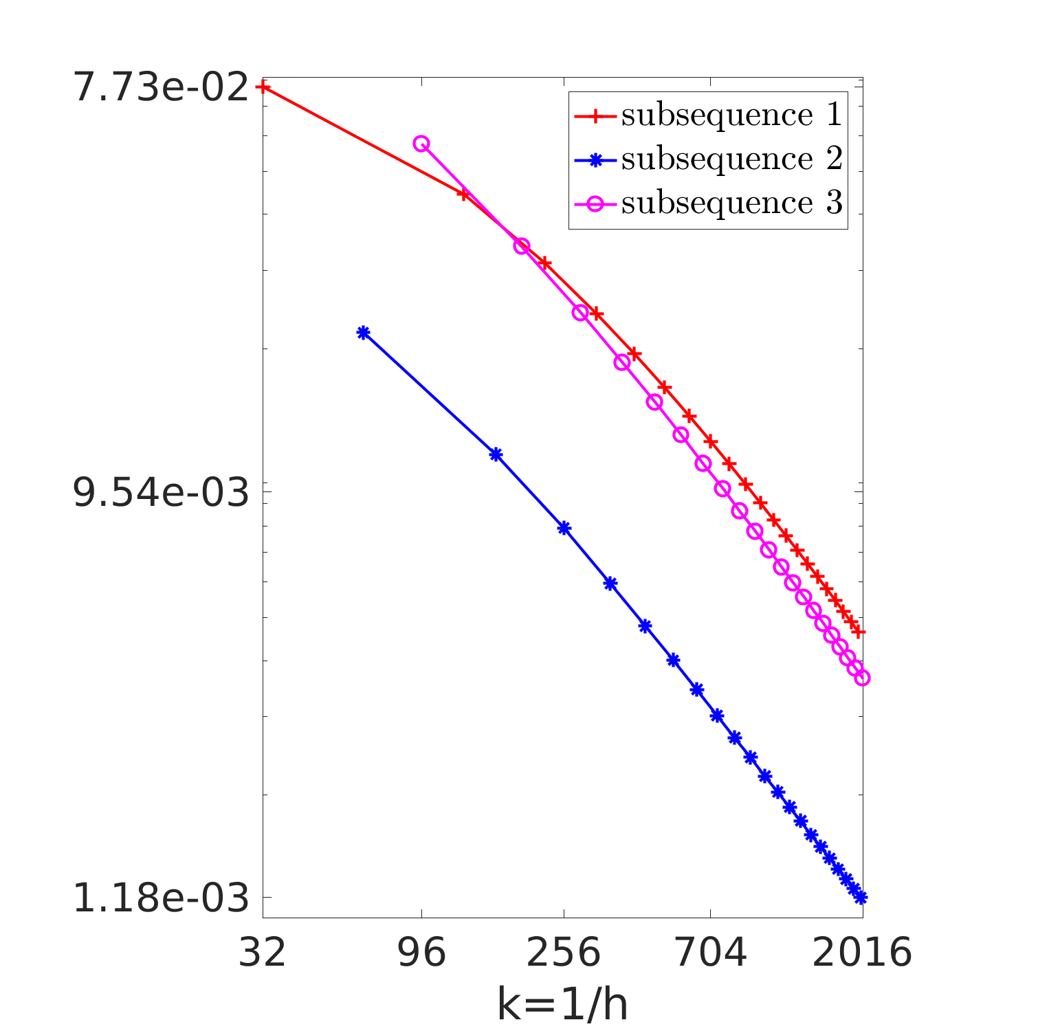
Figure 1: Convergence of different subsequences of Cesàro averages.

Figures 2, 3 present numerical densities computed by the VFV method on $k\times k$ meshes. Figure 4 shows the Cesàro averages of the density for various meshes. Analogous pictures, not presented here, have been obtained also for other summation methods with the weight functions $\omega_{\text{quad}},\ \omega_{\text{sin2}},\ \omega_{\text{exp}}$. The first variance, that is another observable function, is presented for different meshes in Figure 5. More precisely, for the summation method with $\omega_{\text{equal}}$ the first variance is computed as $\frac{1}{k}\sum_{n=1}^{k}\left|{\varrho_{n}}-\frac{1}{k}\sum_{{m}=1}^{k}{\varrho_{m}}\right|.$ In contrast to Figure 2 where no convergence of single numerical solutions is observed, Figures 4, 5 indicate the convergence for observables average and variance.

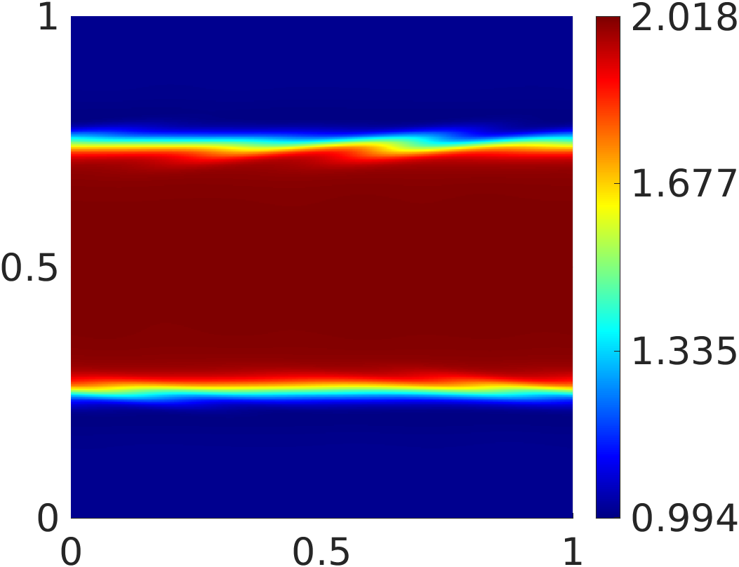
(a) $k=512$

(b) $k=1024$

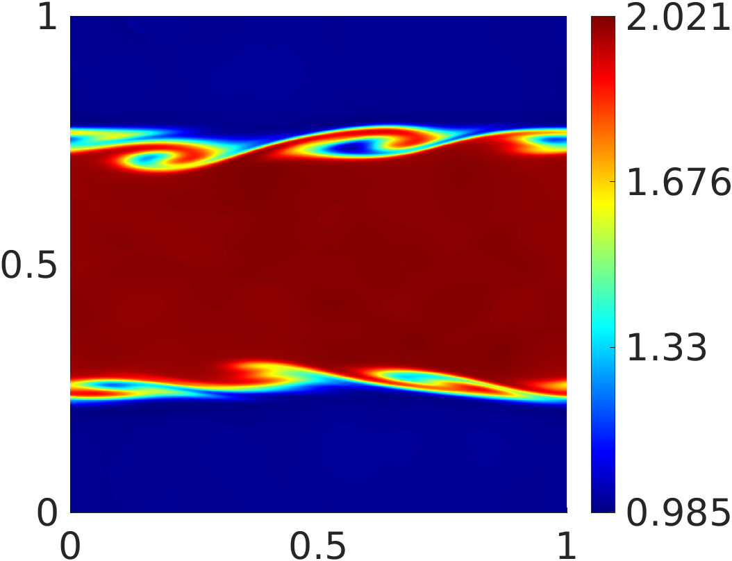
(c) $k=1536$

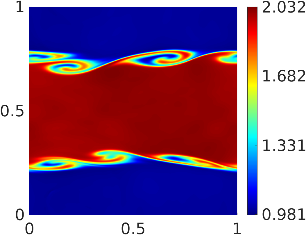
(d) $k=2048$

Figure 2: Density computed by the VFV scheme at $T=2$ for the Kelvin-Helmholtz problem on a mesh with $k\times k$ cells.

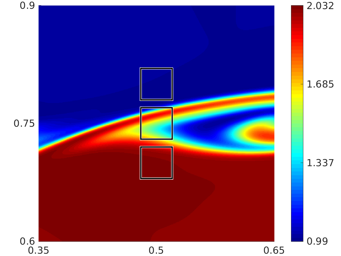
(a) $k=2048$, zoomed in

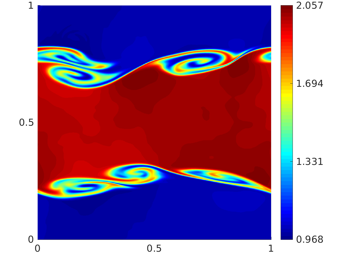
(b) $k=3072$

Figure 3: Density computed by the VFV scheme at $T=2$ for the Kelvin-Helmholtz problem on a mesh with $k\times k$ cells.

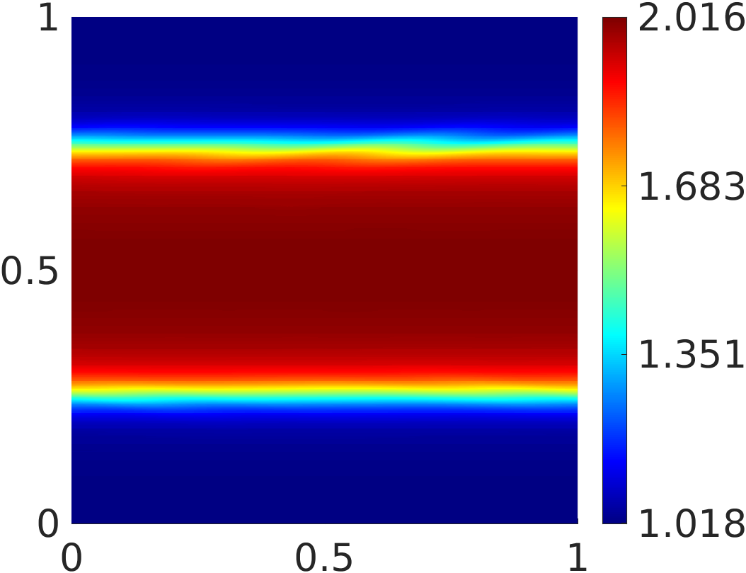
(a) up to $k=512$

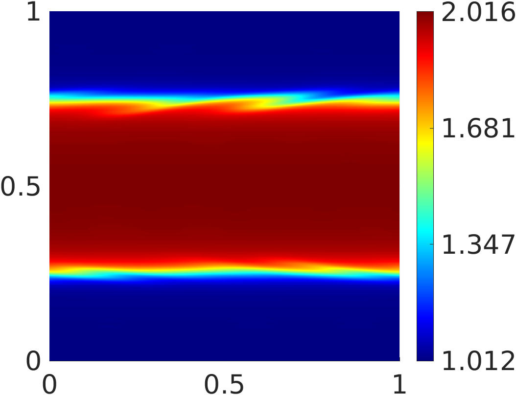
(b) up to $k=1024$

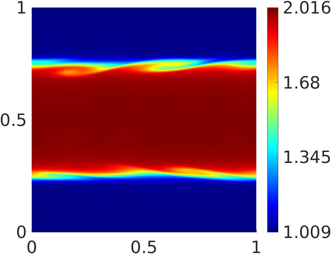
(c) up to $k=1536$

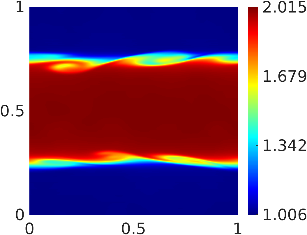
(d) up to $k=2048$

Figure 4: Cesàro averages of the density computed by the VFV method on meshes with $j\times j$ cells, $j=32,\;64,\;96,\dots,\;k$, for the Kelvin-Helmholtz problem.

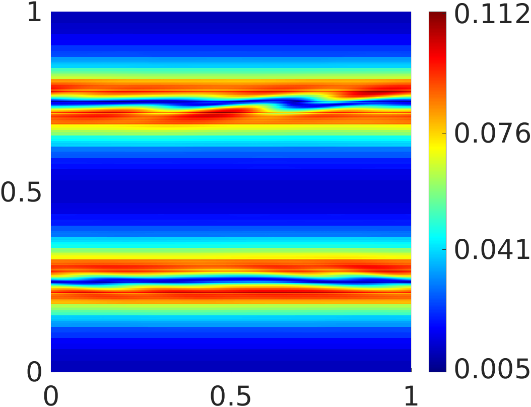
(a) up to $k=512$

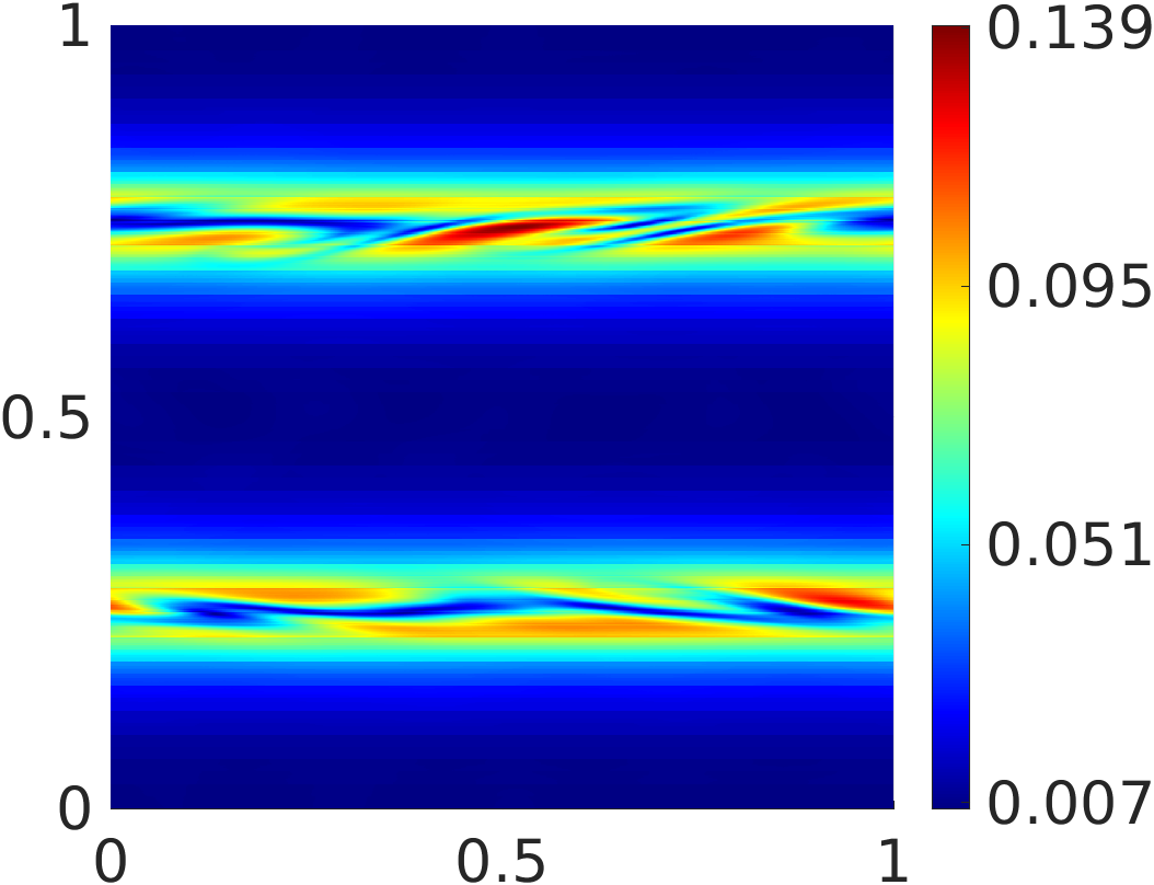
(b) up to $k=1024$

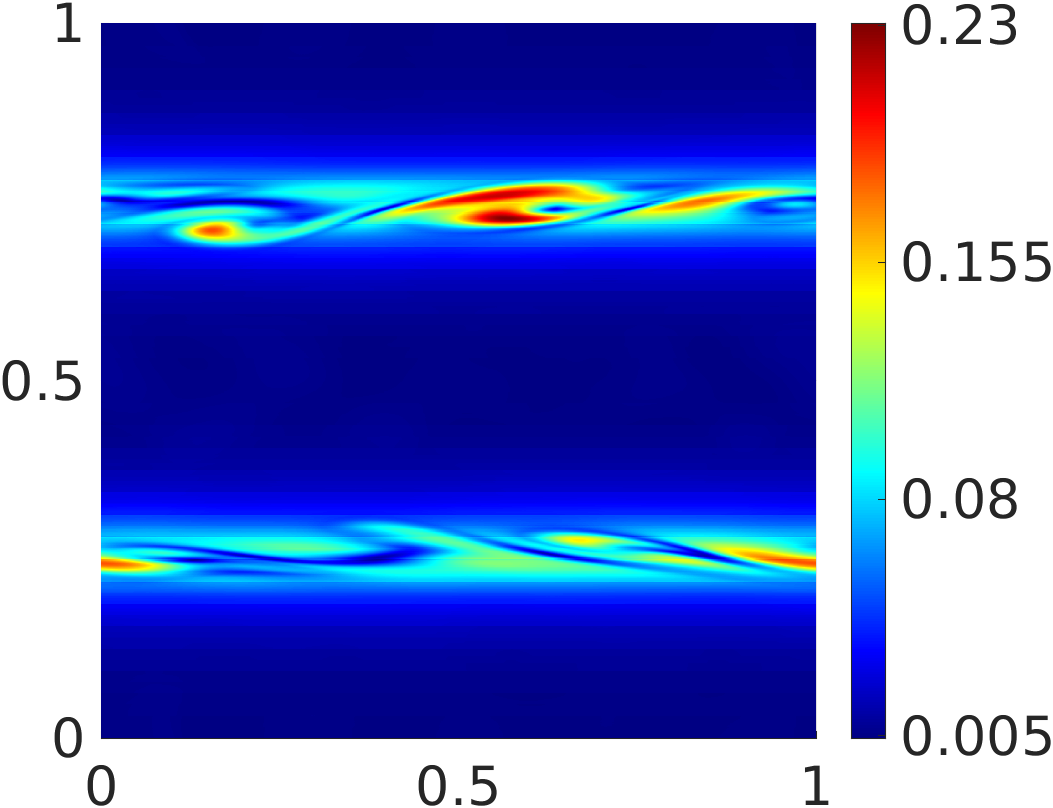
(c) up to $k=1536$

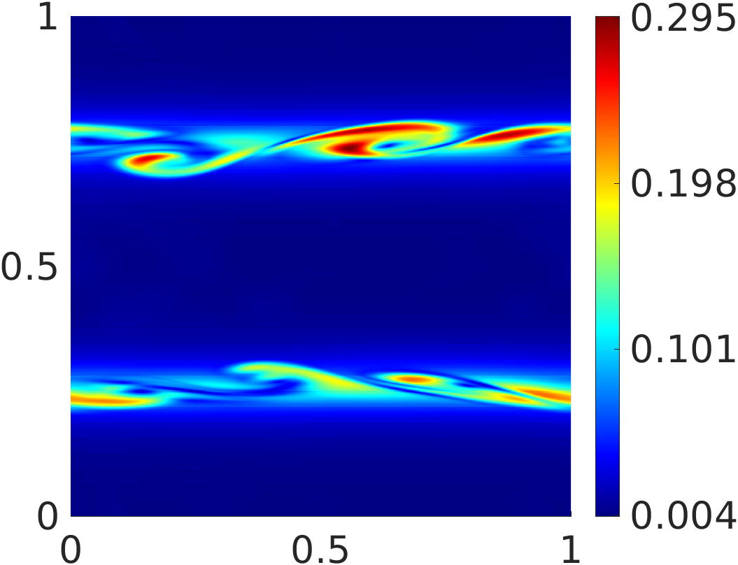
(d) up to $k=2048$

Figure 5: First variance of the density computed by the VFV method on meshes with $j\times j$ cells, $j=32,\;64,\;96,\dots,\;k$, for the Kelvin-Helmholtz problem.

Table 2: Convergence study for different summation methods in the $L^{1}$-norm in space and the Wasserstein distance for measures $\sum_{n=1}^{N}\omega(n/N)\delta_{\varrho_{n}(T,x)}/\sum_{m=1}^{N}\omega(m/N)$ at time $T=2.$

$k$	$\omega_{\text{equal}}$		$\omega_{\text{quad}}$		$\omega_{\text{sin2}}$		$\omega_{\text{exp}}$
(up to)	error	order	error	order	error	order	error	order
48	1.27e-01	-	1.79e-01	-	1.61e-01	-	1.75e-01	-
64	1.05e-01	0.66	1.54e-01	0.52	1.22e-01	0.96	1.50e-01	0.54
96	8.49e-02	0.52	1.35e-01	0.32	9.51e-02	0.61	1.30e-01	0.35
128	6.90e-02	0.72	1.18e-01	0.47	7.51e-02	0.82	1.16e-01	0.40
192	5.49e-02	0.56	1.03e-01	0.34	6.12e-02	0.50	1.03e-01	0.29
256	4.33e-02	0.83	8.92e-02	0.50	5.02e-02	0.69	9.23e-02	0.38
384	3.31e-02	0.66	7.65e-02	0.38	4.11e-02	0.49	8.16e-02	0.30
512	2.47e-02	1.02	6.46e-02	0.59	3.23e-02	0.84	7.07e-02	0.50
768	1.77e-02	0.82	5.34e-02	0.47	2.37e-02	0.76	5.61e-02	0.57
1024	1.24e-02	1.24	4.37e-02	0.70	1.51e-02	1.57	3.32e-02	1.82

To illustrate the probabilistic nature of the limiting solution we present in Figures 6, 7 and 8 the approximations of the probability density at time $T=2$ of the Cesàro averages computed on meshes with $j\times j$ cells, $j\in\{32m\Big{|}\;m\in\mathds{N},\;1\leq m\leq k\}$, averaged in space on the domains $(0.48,0.52)\times(0.68,0.72)$, $(0.48,0.52)\times(0.73,0.77)$ and $(0.48,0.52)\times(0.78,0.82)$, respectively. These three regions are depicted in Figure 3(a). Note that these regions are chosen in such a way that they are either completely below, right on or completely above of the initial upper interface $J_{2}$. These figures yields further evidence of S-convergence as documented in Table 2. The latter presents S-convergence with respect to various summation methods using the weighted functions $\omega_{\text{equal}},\ \omega_{\text{quad}}$, $\omega_{\text{sin2}}$ and $\omega_{\text{exp}}$. In particular, we compute the experimental convergence of the weighted averages $\sum_{n=1}^{N}\omega(n/N)\delta_{\varrho_{n}(T,x)}/\sum_{m=1}^{N}\omega(m/N)$ in the Wasserstein distance. The corresponding reference solutions were obtained using meshes with $k=32,48,64,96,128,192,256,384,512,768,1024,1536,3072$ and the respective weight functions $\omega.$

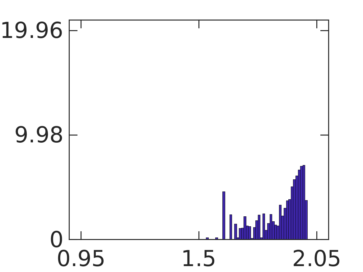
(a) up to $k=512$

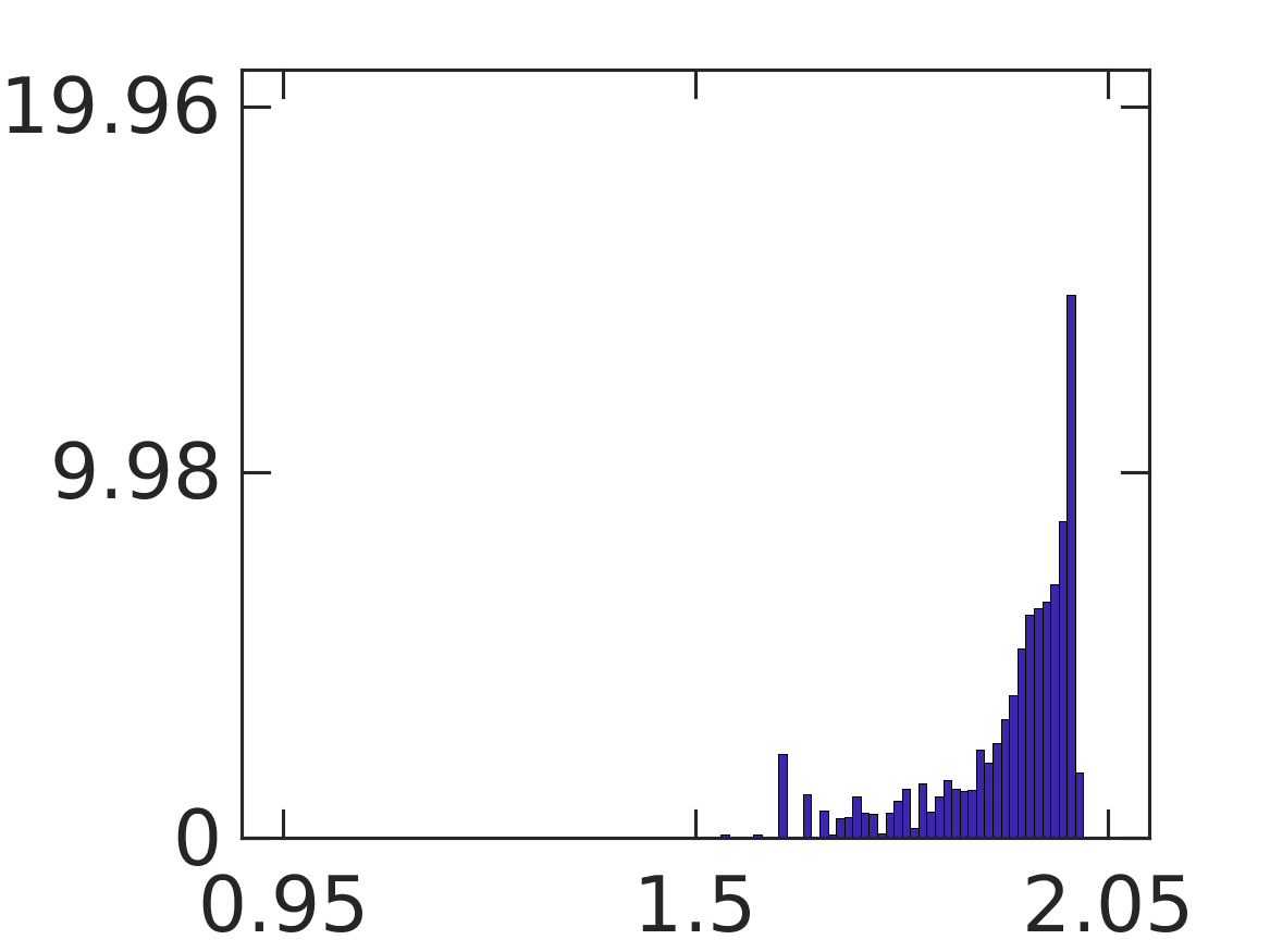
(b) up to $k=1024$

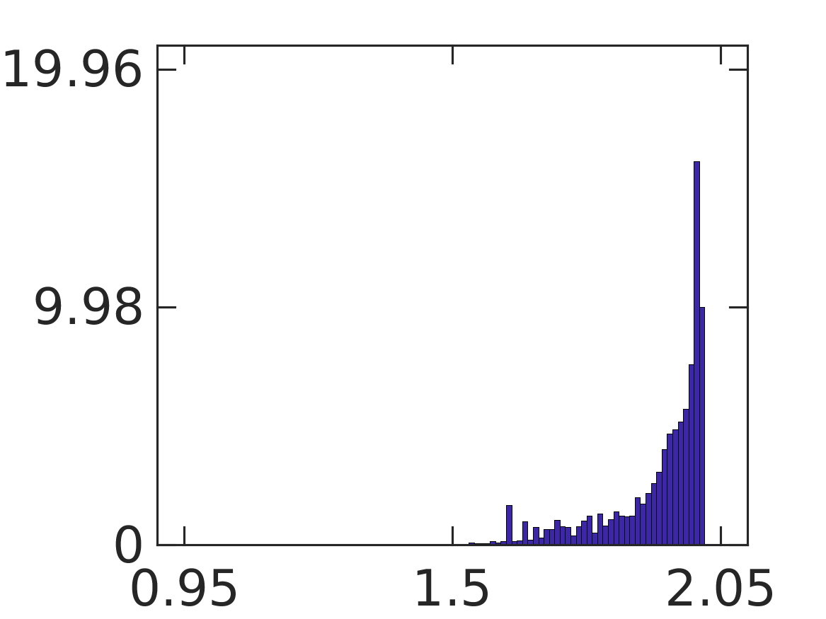
(c) up to $k=1536$

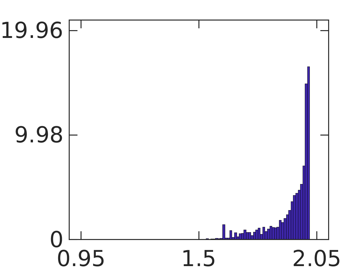
(d) up to $k=1792$

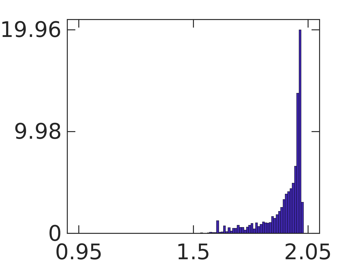
(e) up to $k=2048$

Figure 6: Probability density computed by the VFV method on meshes with $j\times j$ cells, $j=32,\;64,\;96,\dots,\;k$, for the Kelvin-Helmholtz problem on the domain $(0.48,0.52)\times(0.68,0.72)$.

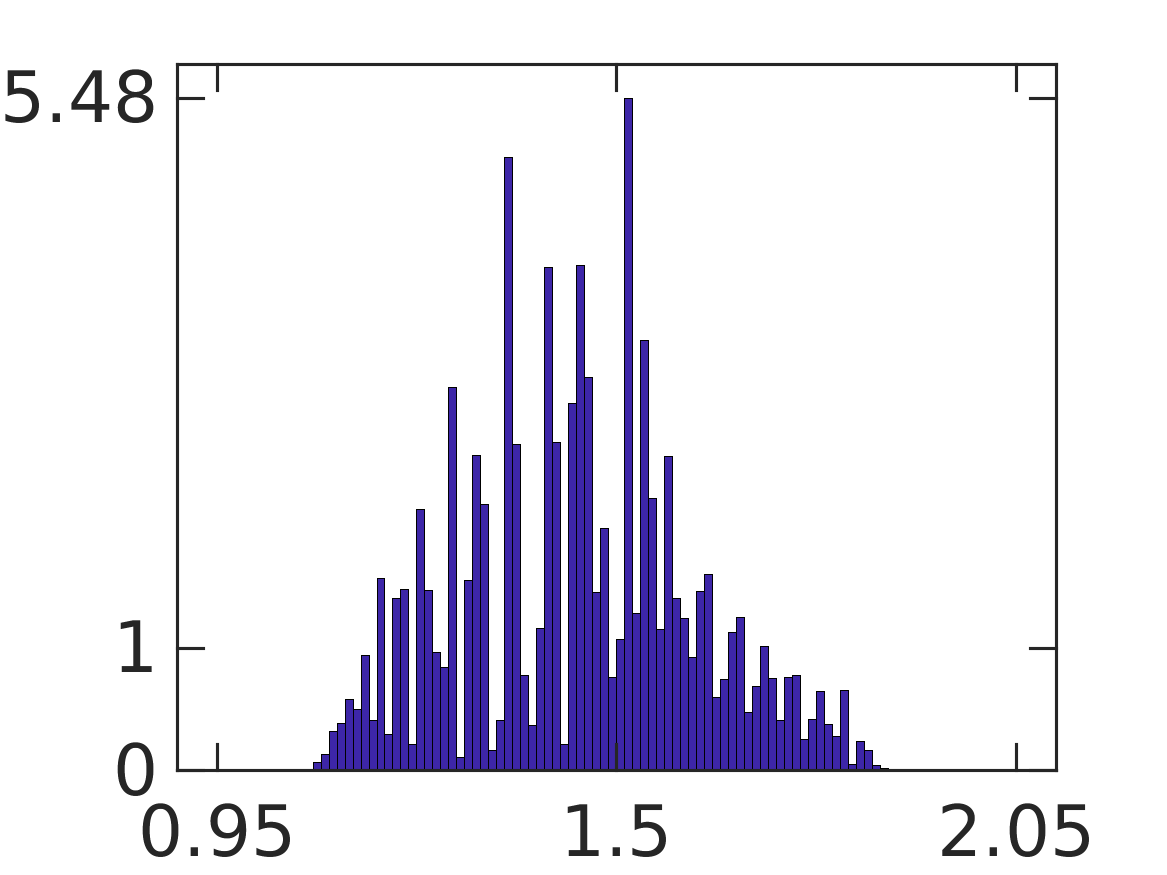
(a) up to $k=512$

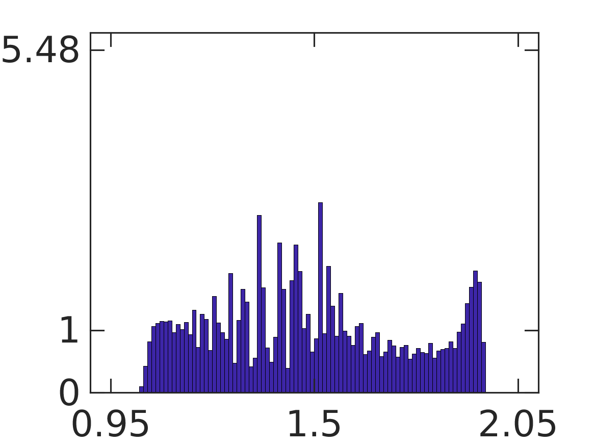
(b) up to $k=1024$

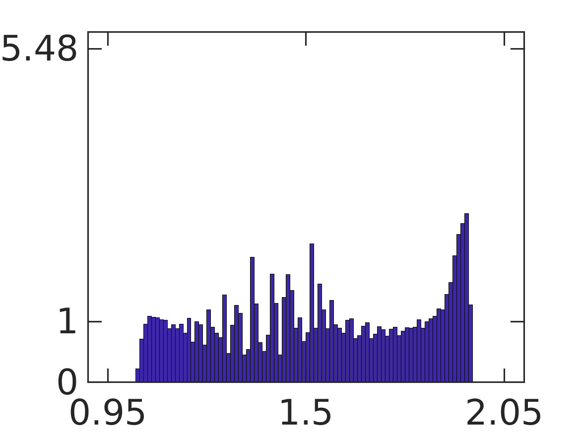
(c) up to $k=1536$

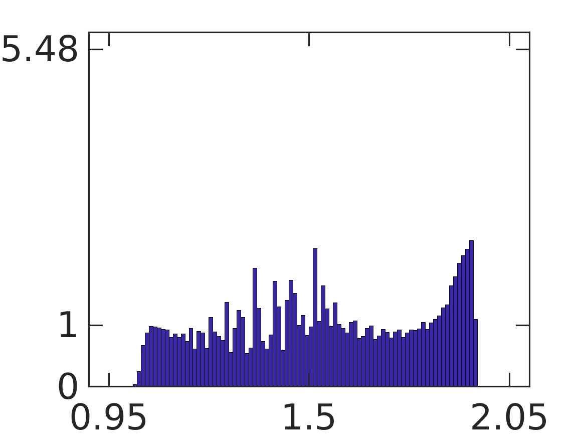
(d) up to $k=1792$

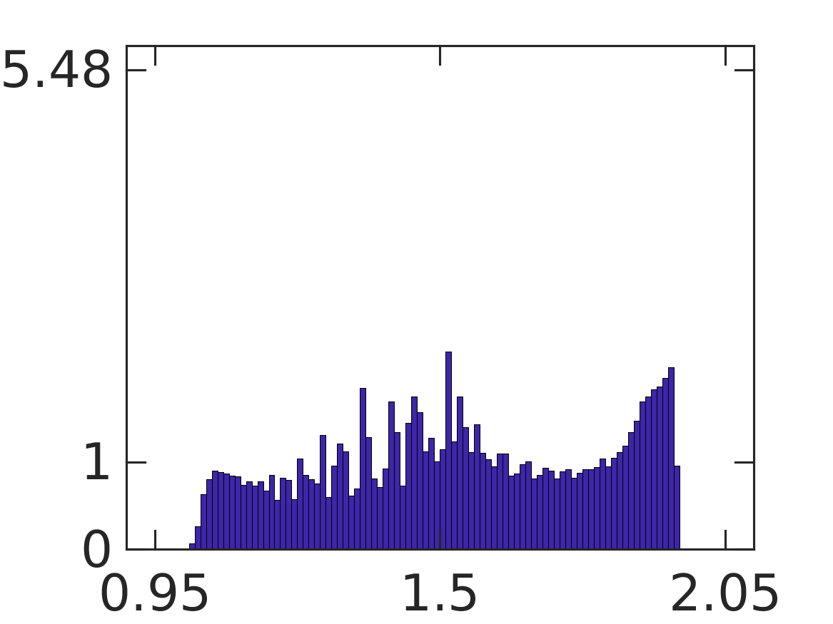
(e) up to $k=2048$

Figure 7: Probability density computed by the VFV method on meshes with $j\times j$ cells, $j=32,\;64,\;96,\dots,\;k$, for the Kelvin-Helmholtz problem on the domain $(0.48,0.52)\times(0.73,{0.77})$.

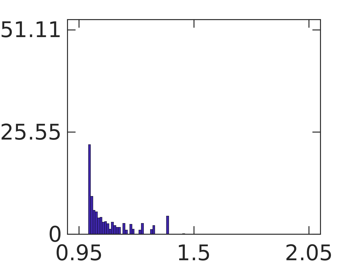
(a) up to $k=512$

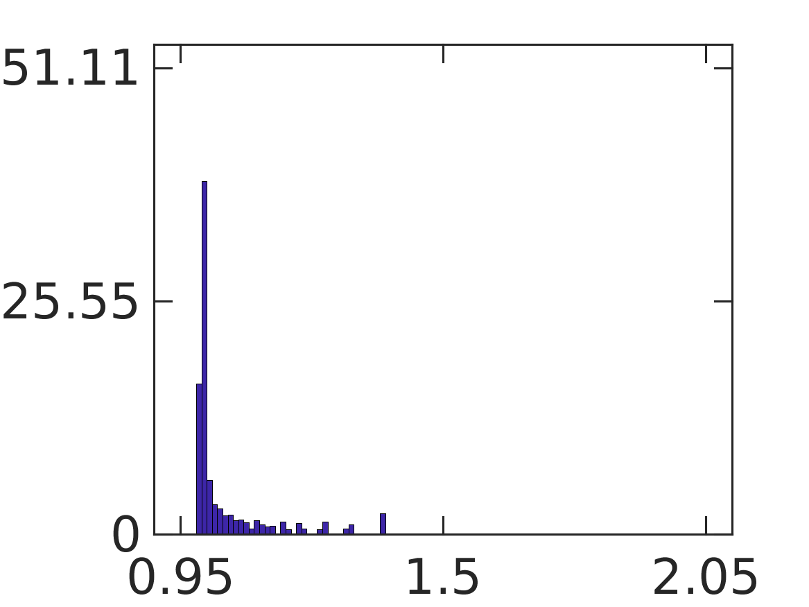
(b) up to $k=1024$

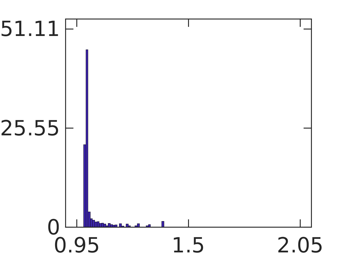
(c) up to $k=1536$

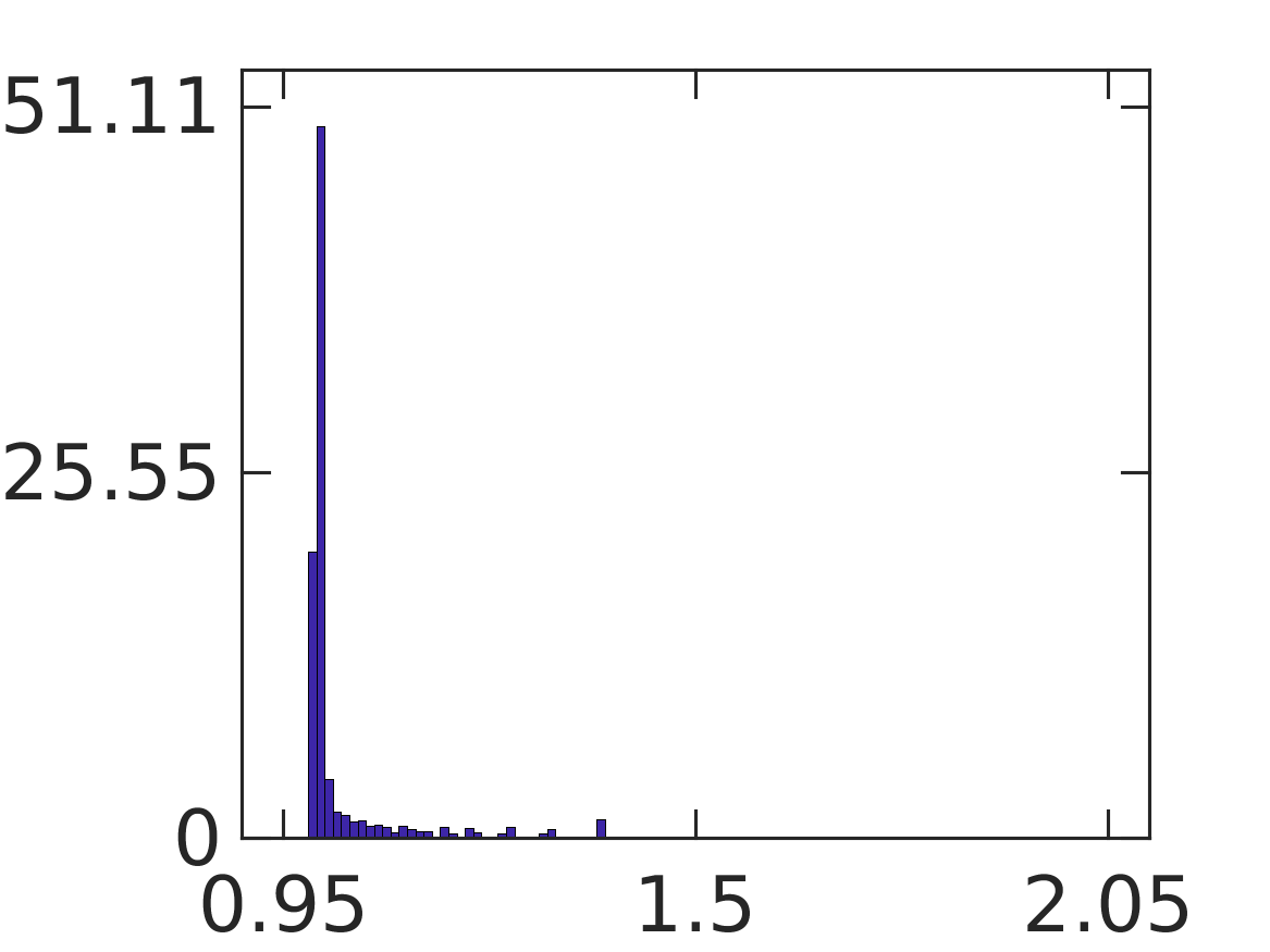
(d) up to $k=1792$

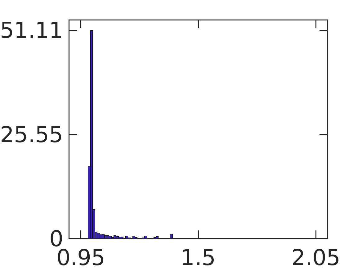
(e) up to $k=2048$

Figure 8: Probability density computed by the VFV method on meshes with $j\times j$ cells, $j=32,\;64,\;96,\dots,\;k$, for the Kelvin-Helmholtz problem on the domain $(0.48,0.52)\times(0.78,0.82)$.

6 Kolmogorov K41 hypothesis

The celebrated Kolmogorov K41 hypothesis for incompressible flow has been extrapolated to the compressible setting by Chen and Glimm [9]. In particular, it yields compactness of any family of (weak) solutions $[\varrho_{n},{\bm{m}}_{n}]_{n=1}^{\infty}$ of the Navier–Stokes system in the zero viscosity regime $\mu_{n}\searrow 0$, $\lambda_{n}\to 0$. This yields strong convergence

$$\varrho_{n_{k}}\to\varrho\ \mbox{in}\ L^{1}((0,T)\times{\mathcal{T}^{d}}),\ {\bm{m}}_{n_{k}}\to{\bm{m}}\ \mbox{in}\ L^{1}((0,T)\times{\mathcal{T}^{d}};\mathds{R}^{d})$$

at least for a suitable subsequence. Thus if $[\varrho,{\bm{m}}]$, or at least ${\bm{m}}$, are observables in the sense of Definition 2.6, the limit is the same for any subsequence. In other words, there is no need of subsequence and the convergence is strong unconditionally. We call this hypothesis (KH). It is easy to check that (KH) yields uniqueness of the viscosity solution,

$${\rm(KH)}\ \Rightarrow\ \mathcal{V}(t,x)=\delta_{[\varrho,{\bm{m}}](t,x)}.$$

We remark that although the convergence of the vanishing viscosity solutions is strong, the limit $[\varrho,{\bm{m}}]$ is not necessarily a weak solution of the Euler system due to possible concentrations.

Now, an easy adaptation of Theorem 5.4 yields:

Theorem 6.1.

Under the hypothesis (KH) let $[\varrho_{h,\mu_{n}},\ {\bm{m}}_{h,\mu_{n}}]$ denote the numerical solution obtained from the VFV method with the initial data $[\varrho_{0,n},{\bm{m}}_{0,n}]$ a regular approximation of $[\varrho_{0},{\bm{m}}_{0}]$, the artificial viscosity $\mu_{n}\searrow 0$, and the numerical step $h$, where $[h,\mu_{n},0]\in\overline{\mathcal{R}}$. Finally, suppose that the condition (5.11) holds for any fixed $\mu_{n}.$

Then there exists $H_{n}\searrow 0$ such that

$$[\varrho_{h_{n},\mu_{n}},{\bm{m}}_{h_{n},\mu_{n}}]\to[\varrho,{\bm{m}}]\ \mbox{in}\ L^{1}((0,T)\times{\mathcal{T}^{d}};\mathds{R}^{d+1})\ \mbox{whenever}\ 0<h_{n}\leq H_{n},$$ (6.1)

where $\delta_{[\varrho,{\bm{m}}]}$ is the unique viscosity solution of the Euler system.

The proof is a combination of Theorem 5.4 for $\mathcal{V}=\delta_{[\varrho,{\bm{m}}]}$ with Lemma 3.8. As a matter of fact, Lemma 3.8 yields (6.1) only for a suitable subsequence, however, the convergence here is unconditional as the limit is unique.

Remark 6.2.

We point out that uniqueness of the limit and its independence of the choice of the sequence of the vanishing viscosity coefficients are imposed in Theorem 6.1 through the (KH) hypothesis.

Remark 6.3.

Note that convergence is unconditional, meaning (5.11) is not required and (6.1) holds for any $H_{n}\to 0$ as soon as the limit $[\varrho,{\bm{m}}]\in C^{1}.$ This follows from Theorem 5.2 and [26, Theorem 5.9].

Unfortunately, the strong convergence to a unique solution is not always observed/expected for compressible fluid flows in the zero viscosity (turbulent) regime. The appearance of the so–called carbuncles observed by Elling [19] or the turbulent wake areas in the obstacle problem are examples of numerous phenomena when, apparently, the convergence to a possible limit is not strong. Such a scenario is compatible with Kolmogorov K41 hypothesis only if the viscosity approximation admits a non–trivial set of accumulation points. In particular, there are different limits for different sequences $\mu_{n}\searrow 0$. Note that this is in sharp contrast with the situation anticipated in Section 2.2, namely the existence of a unique limit of the approximate sequence in the weak topology. The possibility of several limits would obviously invalidate the results of any numerical simulation as the latter sensitively depends on the choice of artificial viscosity and the associated numerical step. Even if S–convergence is applied, the sums

$$\frac{1}{N}\sum_{n=1}^{N}\delta_{(\varrho_{n},{\bm{m}}_{n})(t,x)}$$

may depend on the choice of the approximate sequence.

The only piece of information that could be retained and computed is therefore a statistical limit of the viscous approximation proposed in (1.1). In contrast with the Young measure, the statistical limit is interpreted as a probability measure on the space of solution trajectories, here

$$X=\left\{\varrho,{\bm{m}}\Big{|}\varrho\in C_{\rm weak}([0,T];L^{\gamma}(\Omega)),\ {\bm{m}}\in C_{\rm weak}([0,T];L^{\frac{2\gamma}{\gamma+1}}(\Omega;\mathds{R}^{d}))\right\}.$$

The “statistical” convergence then can be stated as

$$\frac{1}{N}\sum_{n=1}^{N}\delta_{(\varrho_{n},{\bm{m}}_{n})}\to\mathcal{V}\ \mbox{narrowly in}\ \mathfrak{P}[X],$$

which is formally identical with the S–convergence. The standard tools of probability theory, notably the Prokhorov theorem, will provide an analogue of the Subsequence principle stated for S–convergence in Proposition 3.9, namely

$$\frac{1}{N_{k}}\sum_{n=1}^{N_{k}}\delta_{(\varrho_{n},{\bm{m}}_{n})}\to\mathcal{V}\ \mbox{for a suitable subsequence}\ N_{k}\to\infty.$$

Note carefully that here, in contrast with Proposition 3.9, the whole sequence $\{\varrho_{n},{\bm{m}}_{n}\}_{n=1}^{\infty}$ is relevant for the asymptotic limit.

As the statistical limit is associated with a specific choice of the approximate sequence of viscosities and/or initial data, its approximation by the VFV method is possible under the hypotheses of Theorem 5.4. Specifically, we would have to fix the relevant sequence of the data $[\varrho_{0,n},{\bm{m}}_{0,n}]$ together with the viscosities $\mu_{n}\searrow 0$ and to adjust the numerical step $h$ so that $[h,\mu,0]\in\overline{\mathcal{R}}$. This can be CPU demanding since calculation and averaging of large amount of numerical approximations must be realized to obtain a statistically reliable picture.

7 Conclusion

Anticipating the vanishing viscosity limit of the Navier–Stokes system as a physically relevant solution of the Euler system we have identified a viscosity solution of the Euler system with a parametrized family of probability measures generated by solutions of the Navier–Stokes system in the vanishing viscosity limit. We have introduced the observables as the quantities that are independent of a specific approximate sequence and proposed a numerical scheme to compute efficiently the values of observables by means of a summation method. Here efficiently means that the approximate sequence converges strongly (in the $L^{1}$–topology).

Numerical solutions were obtained by the Viscosity Finite Volume method that is based on the standard finite volume method supplemented with vanishing numerical viscosity in the spirit of the model proposed by H. Brenner [2, 3, 4]. We have shown that VFV method identifies the viscosity solution and/or the observables at least if:

• the numerical step $h$ is tuned, in fact considerably smaller than the artificial viscosity $\mu$;

• the VFV method provides a sequence of approximate solutions that admits S–limit if both the numerical step $h$ and the artificial viscosity $\mu$ approach zero.

In future our aim is to study S–convergence for the full Euler system of gas dynamics. A challenging question is to investigate a connection of S–convergence and compressible turbulence.

Appendix

Tables 3 and 4 present the convergence of weighted averages of the density computed on $k\times k$ meshes, with $k=32,\dots,N$, $N\in\{64,\,96,\,128,\,\dots,\,2048\}.$ The reference solution is the same for all summation methods and computed as the Cesàro average of the solutions computed on $k\times k$ meshes with $k\in\{32\ell\,{|}\,\ell\in\mathds{N},\,1\leq\ell\leq 64\}\cup\{2304,2560,2816,3072\}.$

Table 4 presents the convergence results for all weights $\omega$, except $\omega=\omega_{\text{equal}}$, since the computed Cesàro averages are already very close to the reference solution and formally computed experimental order of convergence is not representative.

Table 3: Convergence study in the $L^{1}$-norm for averages of the density at time $T=2$ using different weight functions and the Cesàro average as a reference solution.

$k$	$\omega_{\text{equal}}$		$\omega_{\text{quad}}$		$\omega_{\text{sin2}}$		$\omega_{\text{exp}}$
(up to)	error	order	error	order	error	order	error	order
64	1.44e-01	-	1.92e-01	-	1.92e-01	-	1.92e-01	-
96	1.16e-01	0.54	1.44e-01	0.71	1.44e-01	0.71	1.44e-01	0.71
128	9.72e-02	0.62	1.14e-01	0.81	1.11e-01	0.91	1.07e-01	1.05
160	8.35e-02	0.68	9.34e-02	0.90	8.87e-02	1.01	8.33e-02	1.10
192	7.31e-02	0.73	7.83e-02	0.97	7.33e-02	1.05	6.89e-02	1.04
224	6.50e-02	0.76	6.70e-02	1.01	6.23e-02	1.05	5.85e-02	1.05
256	5.86e-02	0.78	5.85e-02	1.02	5.41e-02	1.06	5.07e-02	1.08
288	5.33e-02	0.80	5.19e-02	1.02	4.77e-02	1.07	4.46e-02	1.09
320	4.90e-02	0.81	4.66e-02	1.02	4.25e-02	1.08	3.98e-02	1.08
352	4.53e-02	0.81	4.23e-02	1.03	3.84e-02	1.07	3.60e-02	1.04
384	4.22e-02	0.81	3.87e-02	1.02	3.50e-02	1.06	3.30e-02	0.98
416	3.96e-02	0.80	3.56e-02	1.02	3.22e-02	1.03	3.07e-02	0.92
448	3.73e-02	0.80	3.31e-02	1.01	3.00e-02	0.99	2.88e-02	0.86
480	3.53e-02	0.80	3.09e-02	0.99	2.81e-02	0.94	2.73e-02	0.79
512	3.35e-02	0.79	2.90e-02	0.97	2.66e-02	0.87	2.60e-02	0.71
544	3.20e-02	0.79	2.74e-02	0.94	2.53e-02	0.80	2.51e-02	0.62
576	3.06e-02	0.78	2.60e-02	0.92	2.43e-02	0.71	2.43e-02	0.53
608	2.93e-02	0.78	2.48e-02	0.88	2.35e-02	0.62	2.37e-02	0.46
640	2.82e-02	0.78	2.38e-02	0.83	2.28e-02	0.54	2.33e-02	0.40
672	2.71e-02	0.77	2.29e-02	0.78	2.23e-02	0.47	2.29e-02	0.35
704	2.62e-02	0.76	2.21e-02	0.73	2.19e-02	0.41	2.26e-02	0.30
736	2.53e-02	0.76	2.15e-02	0.68	2.16e-02	0.36	2.23e-02	0.25
768	2.45e-02	0.77	2.09e-02	0.63	2.13e-02	0.32	2.21e-02	0.22
800	2.37e-02	0.79	2.04e-02	0.58	2.10e-02	0.28	2.19e-02	0.19
832	2.30e-02	0.78	2.00e-02	0.54	2.08e-02	0.25	2.18e-02	0.16
864	2.23e-02	0.80	1.96e-02	0.51	2.06e-02	0.22	2.17e-02	0.13
896	2.17e-02	0.80	1.93e-02	0.47	2.05e-02	0.20	2.16e-02	0.10
928	2.11e-02	0.82	1.90e-02	0.44	2.04e-02	0.18	2.16e-02	0.07
960	2.05e-02	0.84	1.87e-02	0.41	2.03e-02	0.16	2.15e-02	0.05
992	1.99e-02	0.87	1.85e-02	0.39	2.02e-02	0.15	2.15e-02	0.04
1024	1.94e-02	0.89	1.83e-02	0.38	2.01e-02	0.14	2.15e-02	0.03
1056	1.88e-02	0.90	1.81e-02	0.37	2.00e-02	0.13	2.15e-02	0.02

Table 4: Continuation: Convergence study in the $L^{1}$-norm for averages of the density at time $T=2$ using different weight functions and the Cesàro average as a reference solution.

$k$	$\omega_{\text{quad}}$		$\omega_{\text{sin2}}$		$\omega_{\text{exp}}$
(up to)	error	order	error	order	error	order
1088	1.79e-02	0.36	1.99e-02	0.13	2.14e-02	0.02
1120	1.77e-02	0.36	1.98e-02	0.12	2.14e-02	0.03
1152	1.75e-02	0.36	1.98e-02	0.12	2.14e-02	0.03
1184	1.73e-02	0.37	1.97e-02	0.12	2.14e-02	0.04
1216	1.71e-02	0.37	1.96e-02	0.13	2.13e-02	0.06
1248	1.70e-02	0.38	1.96e-02	0.14	2.13e-02	0.07
1280	1.68e-02	0.39	1.95e-02	0.15	2.13e-02	0.09
1312	1.66e-02	0.40	1.94e-02	0.17	2.12e-02	0.11
1344	1.65e-02	0.41	1.93e-02	0.19	2.11e-02	0.13
1376	1.63e-02	0.43	1.92e-02	0.21	2.11e-02	0.15
1408	1.61e-02	0.45	1.91e-02	0.24	2.10e-02	0.17
1440	1.60e-02	0.48	1.90e-02	0.27	2.09e-02	0.19
1472	1.58e-02	0.50	1.89e-02	0.30	2.08e-02	0.21
1504	1.56e-02	0.53	1.87e-02	0.33	2.07e-02	0.24
1536	1.54e-02	0.57	1.86e-02	0.37	2.06e-02	0.26
1568	1.52e-02	0.61	1.84e-02	0.40	2.05e-02	0.30
1600	1.50e-02	0.66	1.83e-02	0.44	2.03e-02	0.33
1632	1.48e-02	0.71	1.81e-02	0.49	2.02e-02	0.36
1664	1.46e-02	0.76	1.79e-02	0.53	2.00e-02	0.40
1696	1.44e-02	0.81	1.77e-02	0.57	1.98e-02	0.44
1728	1.42e-02	0.87	1.75e-02	0.62	1.97e-02	0.47
1760	1.39e-02	0.93	1.73e-02	0.66	1.95e-02	0.51
1792	1.37e-02	0.99	1.71e-02	0.71	1.93e-02	0.55
1824	1.34e-02	1.05	1.69e-02	0.75	1.91e-02	0.59
1856	1.32e-02	1.11	1.66e-02	0.80	1.89e-02	0.62
1888	1.29e-02	1.18	1.64e-02	0.85	1.87e-02	0.66
1920	1.26e-02	1.25	1.61e-02	0.90	1.85e-02	0.70
1952	1.24e-02	1.32	1.59e-02	0.94	1.82e-02	0.73
1984	1.21e-02	1.39	1.56e-02	0.99	1.80e-02	0.77
2016	1.18e-02	1.46	1.54e-02	1.04	1.78e-02	0.80
2048	1.15e-02	1.52	1.51e-02	1.08	1.76e-02	0.83

References

• [1] E. J. Balder. Lectures on Young measure theory and its applications in economics. Rend. Istit. Mat. Univ. Trieste, 31(suppl. 1):1–69, 2000. Workshop on Measure Theory and Real Analysis (Italian) (Grado, 1997).
• [2] H. Brenner. Kinematics of volume transport. Phys. A 349:11–59, 2005.
• [3] H. Brenner. Navier-Stokes revisited. Phys. A 349(1-2):60–132, 2005.
• [4] H. Brenner. Fluid mechanics revisited. Phys. A 349:190–224, 2006.
• [5] A. Bressan and R. Murray. On self-similar solutions to the incompressible Euler equations. J. Differ. Equ. 269(6):5142–5203, 2020.
• [6] T. Buckmaster, C. De Lellis, L. Székelyhidy, and V. Vicol. Onsager’s conjecture for admissible weak solutions. Comm. Pure Appl. Math. 72(2):229-274, 2019.
• [7] T. Buckmaster and V. Vicol. Convex integration and phenomenologies in turbulence. EMS Surv. Math. Sci. 6(1):173–263, 2019.
• [8] G.-Q. Chen and M. Perepelitsa. Vanishing viscosity limit of the Navier-Stokes equations to the Euler equations for compressible fluid flow. Comm. Pure Appl. Math. 63(11):1469–1504, 2010.
• [9] G.-Q. G. Chen and J. Glimm. Kolmogorov-type theory of compressible turbulence and inviscid limit of the Navier-Stokes equations in $\mathbb{R}^{3}$. Phys. D 400:132138, 10, 2019.
• [10] E. Chiodaroli, C. De Lellis, and O. Kreml. Global ill-posedness of the isentropic system of gas dynamics. Comm. Pure Appl. Math. 68(7):1157–1190, 2015.
• [11] E. Chiodaroli, O. Kreml, V. Mácha, and S. Schwarzacher. Non–uniqueness of admissible weak solutions to the compressible Euler equations with smooth initial data. Trans. Amer. Math. Soc. 374:2269–2295, 2021.
• [12] C. De Lellis and L. Székelyhidi, Jr. Dissipative continuous Euler flows. Invent. Math. 193(2):377–407, 2013.
• [13] R. J. DiPerna and A. J. Majda. Concentrations in regularizations for 2-d incompressible flow. Comm. Pure and Appl. Math., 40(3):301–345, 1987.
• [14] R. J. DiPerna and A. J. Majda. Oscillations and concentrations in weak solutions of the incompressible fluid equations. Comm. Math. Phys. 108(4):667–689, 1987.
• [15] R.J. DiPerna and A. Majda. Reduced Hausdorff dimension and concentration cancellation for two-dimensional incompressible flow. J. Amer. Math. Soc. 1:59–95, 1988.
• [16] W. E. Boundary layer theory and the zero-viscosity limit of the Navier-Stokes equation. Acta Math. Sin. (Engl. Ser.) 16(2):207–218, 2000.
• [17] D. B. Ebin. Viscous fluids in a domain with frictionless boundary. Global Analysis - Analysis on Manifolds, H. Kurke, J. Mecke, H. Triebel, R. Thiele Editors, Teubner-Texte zur Mathematik 57, Teubner, Leipzig, 93–110, 1983.
• [18] T. M. Elgindi and I.-J. Jeong. Finite-time singularity formation for strong solutions to the axi-symmetric $3D$ Euler equations. Ann. PDE 5(2): 16, 51, 2019.
• [19] V. Elling. Nonuniqueness of entropy solutions and the carbuncle phenomenon. In Hyperbolic problems: theory, numerics and applications. I, p. 375–382. Yokohama Publ., Yokohama, 2006.
• [20] V. Elling. A possible counterexample to well posedness of entropy solutions and to Godunov scheme convergence. Math. Comp., 75(256):1721–1733, 2006.
• [21] V. Elling. The carbuncle phenomenon is incurable. Acta Math. Sci. Ser. B (Engl. Ed.) 29(6):1647–1656, 2009.
• [22] E. Feireisl. Dynamics of Viscous Compressible Fluids. Oxford University Press, Oxford, 2004.
• [23] E. Feireisl. (S)-convergence and approximation of oscillatory solutions in fluid dynamics. Nonlinearity 34:2327, 2021.
• [24] E. Feireisl and M. Hofmanová. On convergence of approximate solutions to the compressible Euler system. Ann. PDE 6(2):11, 2020.
• [25] E. Feireisl, M. Lukáčová-Medvid’ová, and H. Mizerová. $\mathcal{K}-$convergence as a new tool in numerical analysis. IMA J. Numer. Anal. 40(4): 2227–2255, 2020.
• [26] E. Feireisl, M. Lukáčová-Medvid’ová, H. Mizerová, and B. She. Numerical Analysis of Compressible Fluid Flows. MS&A 20, Springer, 2021.
• [27] E. Feireisl, M. Lukáčová-Medvid’ová, H. Mizerová, and B. She. Convergence of a finite volume scheme for the compressible Navier–Stokes system. ESAIM Math. Model. Numer. Anal. 53(6):1957–1979, 2019.
• [28] E. Feireisl, M. Lukáčová-Medvid’ová, B. She, and Y. Wang. Computing oscillatory solutions to the Euler system via $\mathcal{K}$-convergence. Math. Models Methods Appl. Sci. 31(3):537–576, 2021.
• [29] E. Feireisl, M. Lukáčová-Medvid’ová, and H. Mizerová. A finite volume scheme for the Euler system inspired by the two velocities approach. Numer. Math. 144(1):89–132, 2020.
• [30] H. J. S. Fernando. Turbulent mixing in stratified fluids. Ann. Rev. Fluid Mech. 23: 455-–493, 1991.
• [31] U. K. Fjordholm, R. Käppeli, S. Mishra, and E. Tadmor. Construction of approximate entropy measure valued solutions for hyperbolic systems of conservation laws. Found. Comput. Math. 17(3):763–827, 2017.
• [32] U. S. Fjordholm, S. Mishra, and E. Tadmor. On the computation of measure-valued solutions. Acta Numer. 25:567–679, 2016.
• [33] J.-L. Guermond and B. Popov. Viscous regularization of the Euler equations and entropy principles. SIAM J. Appl. Math. 74(2):284–305, 2014.
• [34] H. von Helmhotz. On the discontinuous movements of fluids. Monatsberichte der Königlichen Preussische Akademie der Wissenschaften zu Berlin 23: 215–278, 1868.
• [35] P. Isett. A proof of Onsager’s conjecture. Ann. of Math. (2) 188(3):871–963, 2018.
• [36] W.T. Kelvin. Hydrokinetic solutions and observations. Philosophical Magazine 42: 362–377, 1871.
• [37] P.-L. Lions. Mathematical Topics in Fluid Dynamics, Vol.2, Compressible models. Oxford Science Publication, Oxford, 1998.
• [38] A. Matsumura and T. Nishida. The initial value problem for the equations of motion of compressible and heat conductive fluids. Comm. Math. Phys. 89:445–464, 1983.
• [39] P. I. Plotnikov and W. Weigant. Isothermal Navier-Stokes equations and Radon transform. SIAM J. Math. Anal. 47(1):626–653, 2015.
• [40] H. P. Rosenthal. Weakly independent sequences and the Banach–Saks property. In Proceedings of the Durham Symposium on the relations between infinite dimensional and finite dimensional convexity, p. 26. Durham, 1975.
• [41] Y. Sun, C. Wang, and Z. Zhang. A Beale-Kato-Majda criterion for three dimensional compressible viscous heat-conductive flows. Arch. Ration. Mech. Anal. 201(2):727–742, 2011.
• [42] A. Valli and M. Zajaczkowski. Navier-Stokes equations for compressible fluids: Global existence and qualitative properties of the solutions in the general case. Commun. Math. Phys. 103:259–296, 1986.
• [43] C. Villani. Optimal Transport, Old and New., volume 338 of Grundlehren der Mathematischen Wissenschaften [Fundamental Principles of Mathematical Sciences]. Springer-Verlag, Berlin, 2009.