Multi-valued inverse design: multiple surface geometries from one flat sheet

Abstract

Designing flat sheets that can be made to deform into 3D shapes is an area of intense research with applications in micromachines, soft robotics, and medical implants. Thus far, such sheets were designed to adopt a single target shape. Here, we show that through anisotropic deformation applied inhomogenously throughout a sheet, it is possible to design a single sheet that can deform into multiple surface geometries upon different actuations. The key to our approach is development of an analytical method for solving this multi-valued inverse problem. Such sheets open the door to fabricating machines that can perform complex tasks through cyclic transitions between multiple shapes. As a proof of concept we design a simple swimmer capable of moving through a fluid at low Reynolds numbers.

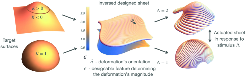
Figure 1: Inverse design of pluripotent sheets. Left: Target surfaces with defined Gaussian curvatures $K$. Center: Inverse designed sheet. $\hat{\mathbf{n}}$ specifies the deformation’s orientation. $\epsilon$ is an experimentally accessible system feature controlling the deformation’s magnitude which is designed with $\hat{\mathbf{n}}$ such that the sheet deforms into the target surfaces. Right: Actuated sheet deforming into multiple target surfaces in response to different values of the stimulus $\Lambda$.

Designing shape shifting sheets is of enormous interest in fields including micromachines Miskin et al. (2020), soft robotics Reyssat and Mahadevan (2009); Wallin et al. (2018), and medical implants Teo et al. (2016) where fabrication and production constraints often require an initial flat configuration. Programming a single shape transformation in such sheets already enables designs for switches, deployable structures Hartl and Lagoudas (2007), and actuators Guin et al. (2018). Designing sheets that can adopt multiple target geometries would open the door to more sophisticated machines that can cycle through multiple states, perform work on their surroundings, and locomote through viscous fluids Palagi and Fischer (2018); Levin et al. (2020).

In origami it is possible to program more than one shape into a single sheet Demaine and Tachi (2017); Na et al. (2015); Liu et al. (2021a). However, the shapes are almost always incompatible, which means that the sheet must return to the flat configuration before it is folded into another shape. Elastic sheets can fold from one shape to another directly Manna et al. (2020). Here, we show how to inverse design a sheet so that it can transform into a series of shapes in an arbitrary sequence in response to actuation signals. By transforming from one shape to another directly, without returning to its original flat configuration, such sheets are able to perform complex tasks and do work on their environment. The challenge in designing such pluripotent sheets, however, is that one must simultaneously control multiple independent degrees of freedom, such as the deformation magnitude and orientation, to obtain multiple independent shapes (Fig. 1).

Most shape shifting sheets have been designed to deform into a single target geometry via one of two deformation modalities where only one deformation degree of freedom is varied Modes and Warner (2016): $(\mathrm{i})$ inhomogeneous isotropic deformations Korn (1914); Lichtenstein (1916), where the deformation magnitude varies throughout the sheet Kim et al. (2012a); Pikul et al. (2017); Kim et al. (2012b); Klein et al. (2007); and $(\mathrm{ii})$ homogeneous anisotropic deformations Griniasty et al. (2019), where the deformation principal axis varies throughout the sheet Fahn and Zohary (1955); Armon et al. (2011); Reyssat and Mahadevan (2009); Aharoni et al. (2012, 2014); Mostajeran (2015); Sydney Gladman et al. (2016); Ware et al. (2015); Mostajeran et al. (2016); Aharoni et al. (2018); Warner and Mostajeran (2018); Kowalski et al. (2018); Siéfert and Warner (2020); Duffy and Biggins (2020); Feng et al. (2020). Both modalities can be used to alter a sheet’s local Gaussian curvature and determine its geometry. Importantly, the technology to simultaneously implement both modalities to achieve multiple shapes already exists Pikul et al. (2017); Siéfert et al. (2019). Missing, however, is a mathematical framework to generate designs that implement both degrees of freedom to obtain the desired surfaces.

Naive combinations of the inverse design methods of homogeneous and anisotropic systems Korn (1914); Lichtenstein (1916); Griniasty et al. (2019) generally fail at this task. The naive approach fails because the local Gaussian curvature of an actuated sheet is nonlinearly dependent on both degrees of freedom. The curvature is, however, linear in the highest order derivatives of the deformation degrees of freedom. Therefore, it may be possible to rephrase the inverse design problem as a system of PDEs in the deformation degrees of freedom, where the actuated sheet’s curvatures equal those of the target surfaces, and use linearity to simultaneously solve the equations.

Implementing this strategy requires formulating a common description of the initial and target surfaces in terms of a shared coordinate system. A sheet’s deformation is characterized by its principal axis with respect to the initial sheet, denoted by a director $\hat{\mathbf{n}}$, and the deformation magnitudes along and across the director $\lambda_{1}$ and $\lambda_{2}$ respectively. Generally $\lambda_{1},\lambda_{2}$, and $\hat{\mathbf{n}}$ can all depend on external time dependent actuation stimuli ${\bm{\Lambda}}(t)$ that drive the deformation. Most known anisotropically deforming systems, however, are uniaxial: their deformation’s principal axis $\hat{\mathbf{n}}$ is independent of the actuation ${\bm{\Lambda}}$ Fahn and Zohary (1955); Armon et al. (2011); Reyssat and Mahadevan (2009); Aharoni et al. (2012, 2014); Mostajeran (2015); Sydney Gladman et al. (2016); Ware et al. (2015); Mostajeran et al. (2016); Aharoni et al. (2018); Warner and Mostajeran (2018); Kowalski et al. (2018); Siéfert and Warner (2020); Duffy and Biggins (2020); Feng et al. (2020); Giudici and Biggins (2021). In such materials the integral curves of the principal axis $\hat{\mathbf{n}}$ and its perpendicular $\hat{\mathbf{n}}_{\perp}$ form a ‘material’ coordinate system $(u,v)$ on the sheet throughout the deformation such that

$${\partial_{u}{\mathbf{r}_{{\bm{\Lambda}}}}=\alpha\lambda_{1}{\hat{\mathbf{n}}_{\bm{\Lambda}}},\quad\partial_{v}{\mathbf{r}_{\bm{\Lambda}}}=\beta\lambda_{2}\hat{\mathbf{n}}_{{\bm{\Lambda}}\perp}}$$ (1)

where $\mathbf{r}_{\bm{\Lambda}}$ are the coordinates of the sheet for an actuation ${\bm{\Lambda}}$, $\alpha$ and $\beta$ are the arc lengths of $u$ and $v$ parametric curves on the initial sheet, and ${\hat{\mathbf{n}}}_{\bm{\Lambda}}$ are the images of the director $\hat{\mathbf{n}}$ on the deformed surfaces (Fig. 2). The deformation magnitudes are also functions of designable features $\bm{\epsilon}(u,v)$ specified on the undeformed sheet. Thus the sheets’ geometries throughout the deformation are given by the metrics

$$ds^{2}(\mathbf{\Lambda})=\lambda_{1}^{2}(\mathbf{\Lambda},\bm{\epsilon})\alpha^{2}du^{2}+\lambda_{2}^{2}(\bm{\Lambda},\bm{\epsilon})\beta^{2}dv^{2}.$$ (2)

This shared coordinate system can then be used to define the Gaussian curvatures of multiple actuated surfaces simultaneously.

An actuated sheet’s Gaussian curvature is a function of the deformation degrees of freedom expressed in the metric, Eq. (2), and its derivatives. For a surface with orthogonal coordinates defined by Eq. (1) the Gaussian curvature is given by Niv and Efrati (2018):

$${K=\hat{\mathbf{n}}_{\perp}\cdot\nabla\kappa_{gu}-\hat{\mathbf{n}}\cdot\nabla\kappa_{gv}-\kappa_{gu}^{2}-\kappa_{gv}^{2}}.$$

where $\kappa_{gu}$ and $\kappa_{gv}$ are geodesic curvatures of $u$ and $v$ parametric curves, which are themselves PDEs in the designable director:

$$\kappa_{gu}\hat{\mathbf{n}}_{\perp}=\hat{\mathbf{n}}\cdot\nabla\hat{\mathbf{n}},\quad\quad\kappa_{gv}\hat{\mathbf{n}}_{\perp}=\hat{\mathbf{n}}_{\perp}\cdot\nabla\hat{\mathbf{n}}.$$ (3)

Keeping in mind that we would eventually like to design the sheet properties, we express the geodesic curvatures, $\kappa_{gu}$ and $\kappa_{gv}$, as functions of the designable elastic features $\bm{\epsilon}$, as well as $\alpha$ and $\beta$ which uniquely determine the designable director $\hat{\mathbf{n}}$ Niv and Efrati (2018) (see supplemental material (SM) for derivation SM ):

$$\kappa_{gu}=\frac{b}{\lambda_{2}}-\frac{\partial\lambda_{1}}{\lambda_{1}\partial\bm{\epsilon}}\frac{\mathbf{q}}{\lambda_{2}},\quad\kappa_{gv}=\frac{s}{\lambda_{1}}+\frac{\partial\lambda_{2}}{\lambda_{2}\partial\bm{\epsilon}}\frac{\mathbf{p}}{\lambda_{1}},$$ (4)

$$b=-\frac{\partial_{v}\alpha}{\alpha\beta},\quad s=\frac{\partial_{u}\beta}{\alpha\beta},\quad\mathbf{p}=\frac{\partial_{u}\bm{\epsilon}}{\alpha}\text{ and }\mathbf{q}=\frac{\partial_{v}\bm{\epsilon}}{\beta}.$$

Derivatives along and across the director are expressed with respect to $u$ and $v$: $\hat{\mathbf{n}}\cdot\nabla=\frac{1}{\lambda_{1}\alpha}\partial_{u}$ and $\hat{\mathbf{n}}_{\perp}\cdot\nabla=\frac{1}{\lambda_{2}\beta}\partial_{v}$. Using Eq. (4), we can thus express the Gaussian curvature as a quasi-linear first order equation in $b,s,\mathbf{p}$ and $\mathbf{q}$,

$$K=-\left(\frac{s}{\lambda_{1}}+\frac{\partial\lambda_{2}}{\lambda_{2}\partial\bm{\epsilon}}\frac{\mathbf{p}}{\lambda_{1}}\right)^{2}-\left(\frac{b}{\lambda_{2}}-\frac{\partial\lambda_{1}}{\lambda_{1}\partial\bm{\epsilon}}\frac{\mathbf{q}}{\lambda_{2}}\right)^{2}+$$ (5)

$$\frac{1}{\lambda_{2}\beta}\frac{\partial}{\partial v}\left(\frac{b}{\lambda_{2}}-\frac{\partial\lambda_{1}}{\lambda_{1}\partial\bm{\epsilon}}\frac{\mathbf{q}}{\lambda_{2}}\right)-\frac{1}{\lambda_{1}\alpha}\frac{\partial}{\partial u}\left(\frac{s}{\lambda_{1}}+\frac{\partial\lambda_{2}}{\lambda_{2}\partial\bm{\epsilon}}\frac{\mathbf{p}}{\lambda_{1}}\right).$$

The quantities $b,s,{\mathbf{p}}$ and ${\mathbf{q}}$, and by extension the Gaussian curvature, are thus determined by $\bm{\epsilon}$, $\alpha$ and $\beta$.

Since $\bm{\epsilon}$, $\alpha$ and $\beta$ are independent, the relations in Eq. 4 allow for the simultaneous satisfaction of Eq. (5) for multiple surface geometries. To obtain solutions, this system of PDEs must be diagonalized, and shown to be integrable. We illustrate this procedure for a flat sheet that deforms into two different target shapes, and show how it naturally extends for an arbitrary number of target shapes.

Inverse design of two target surfaces: Consider a uniaxial sheet with a single scalar designable feature $\epsilon$ affecting the deformation such that, without loss of generality , $\partial_{\epsilon}\lambda_{1}\neq 0$. The curvatures of the initial sheet and two target surface geometries $\mathbf{K}=(K_{0}(\mathbf{r}_{\Lambda_{0}}),K_{1}(\mathbf{r}_{\Lambda_{1}}),K_{2}(\mathbf{r}_{\Lambda_{2}}))$ define 3 PDEs in $\epsilon,\alpha$ and $\beta$. The equations are linear in $\partial_{v}b,\partial_{u}s,\partial_{u}p$ and $\partial_{v}q$. The variations of $\epsilon$, $\partial_{u}p$ and $\partial_{v}q$, however, are not independent, and as shown in the SM SM $\partial_{v}q$ determines $\partial_{u}p$ given a Cauchy problem Hadamard (1923). Recasting Eq. (5) in terms of the unknown highest order terms

$$\bar{\mathbf{K}} =\mathbf{K}-\mathbf{M}\cdot\mathbf{d},$$ (6)

$$M_{i}(\Lambda_{i}) =\begin{pmatrix}\frac{1}{\lambda_{2}^{2}}&-\frac{1}{\lambda_{1}^{2}}&-\frac{\partial\log\lambda_{1}}{\lambda_{2}^{2}\partial\epsilon}\end{pmatrix},\quad i\in\{1,2,3\},$$

$$\mathbf{d} =\begin{pmatrix}\frac{1}{\beta}\partial_{v}b&\frac{1}{\alpha}\partial_{u}s&\frac{1}{\beta}\partial_{v}q\end{pmatrix},$$

it is possible to determine $\partial_{v}b,\partial_{u}s$ and $\partial_{v}q$ in terms of $\bar{\mathbf{K}}$ which are functions of $(\alpha,\beta,\epsilon,p,q,b,s$ and $\partial_{u}p)$ and the prescribed target curvatures $\mathbf{K}$:

$$\mathbf{d}=\mathbf{M}^{-1}\cdot(\mathbf{K}-\bar{\mathbf{K}}).$$ (7)

Equations (1,3,4) and (7) form a system of PDEs, whose solution is a uniaxial sheet that deforms into the two desired target surfaces upon actuations $\Lambda_{1}$ and $\Lambda_{2}$ (see Fig. 1). Supplemented by analytical initial conditions, this system is complete and integrable Evans (2010); SM . Furthermore, if one of the deformation magnitudes is insensitive to $\epsilon$, which is the case for existing implementations of uniaxial sheets Pikul et al. (2017); Siéfert et al. (2019), the system of equations is hyperbolic, and a solution can be integrated from initial conditions for a substantial domain Press et al. (2007).

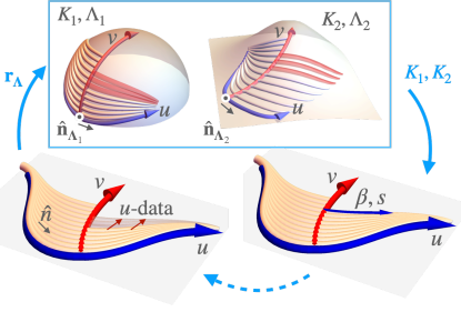
Figure 2: Inverse design scheme of a flat uniaxial sheet with a designable elastic response, $\lambda_{1}(\epsilon)\neq\mathrm{const},$ for two target surfaces with Gaussian curvatures $K_{1}$ and $K_{2}$ in response to stimuli $\Lambda_{1}$ and $\Lambda_{2}$. The $(u,v)$ coordinates given by the integral curves of the deformation’s anisotorpy axis $\hat{\mathbf{n}}$ or $\hat{\mathbf{n}}_{\perp}$, are shared by all surfaces and and allow the derivation of a system of equations describing the inverse problem. A numerical integration of this inverse problem is given by iteration of the following integration steps. Bottom left: Given complete data on a director integral curve, $u\text{-data}=(\mathbf{r}_{\Lambda},\hat{\mathbf{n}}_{\Lambda},\alpha,b,\epsilon,q)$ is propagated a step $dv$ along the director perpendicular, forming a new director integral curve. Top: The curvature of the target surfaces along the new director integral curve is obtained. Bottom right: Initial data for $\beta$ and $s$, given on the initial director-perpendicular curve, is integrated along the new director integral curve to complete the data on it.

It is illuminating to find solutions of the inverse problem, $\bm{\epsilon}(\mathbf{r})$ and $\hat{\mathbf{n}}(\mathbf{r})$, by integrating a Goursat-like problem Goursat (1923) as depicted in Fig. 2. Initial data consists of a position and director on each target surface, accompanied by $u$ and $v$ curves on the initial surface, where data propagating across each curve is given on it. That is, data for $(\alpha,b,\epsilon,q)$ is given on the $u$-curve, and data for $(\beta,s)$ is given on the $v$-curve. A solution is then found by iteratively propagating the data along $u$ and $v$. The variables $u\text{-data}\equiv\left(\alpha,\epsilon,b,p,\partial_{v}p,q,\{\mathbf{r}_{{\bm{\Lambda}}_{i}},\hat{\mathbf{n}}_{{\bm{\Lambda}}_{i}}\}_{i=0}^{2}\right)$ are propagated a step $dv$, forming a new $u$-curve. Next, the curvatures of the target surfaces $(K_{1}(\mathbf{r}_{\Lambda_{1}}),K_{2}(\mathbf{r}_{\Lambda_{2}}))$ are obtained along the new curve. With these curvatures we obtain the values of $\partial_{u}s$ through Eq. (7), which we integrate to obtain $s$ and $\beta$ along the new $u$-curve, completing the data on it. The integration steps are iterated until a global solution of the inverse problem, $\epsilon(\mathbf{r}),\hat{\mathbf{n}}(\mathbf{r})$ is found, or until a singularity forms: $\alpha=0$, $\beta=0$, or for all applied stimuli $\lambda_{1}=\lambda_{2}$.

Singularities: The first two singularities where $\alpha$ or $\beta$ vanish are defects in the nematic texture discussed in Griniasty et al. (2019). The third, $\lambda_{1}=\lambda_{2}$ for all applied stimuli, is an isotropic point. At such a point variations of the director no longer affect the deformation, and the sheet cannot be designed to obtain all target curvatures simultaneously. The appearance of singularities may be delayed by varying the initial conditions, such that greater coverage of the target surfaces is achieved Griniasty et al. (2019).

Inverse design of multiple surfaces: In general, if there are $N$ designable features, $\bm{\epsilon}$, independently affecting a uniaxial sheet’s deformation, then the sheet may be designed to morph into $N+1$ independent surfaces. Here, the inverse design procedure is nearly identical to that of a sheet morphing into two shapes. The key difference is that because there are multiple designable features, we can no longer assume that they all affect the deformations along the director. For example, if $\epsilon_{1}$ affects only the deformation along the director, $\lambda_{1}$, while $\epsilon_{2}$, affects only the deformation across it, $\lambda_{2}$, then the variations of $\epsilon_{1}$ across the director, and $\epsilon_{2}$ along it, $\partial_{v}q_{1}$ and $\partial_{u}p_{2}$, are relevant to their inverse design, while $\partial_{u}p_{1}$ and $\partial_{v}q_{2}$ are not. Equation (6) then needs to be modified to account for the relevant highest order terms, ${\mathbf{d}}$, which now include $\partial_{v}b,\partial_{u}s$ and a mix of $\partial_{u}p_{i}$ and $\partial_{v}q_{j}$. The coefficients matrix ${\mathbf{M}}$ is then appropriately redefined, such that after subtracting ${\mathbf{M}}\cdot{\mathbf{d}}$ from the curvature ${\mathbf{K}}$, the remainder $\bar{{\mathbf{K}}}$ is no longer a function of the relevant highest order derivatives. The accordingly modified Eq.(7), together with Eqns. (1,3) and (4) then compose a complete, integrable system of equations whose solutions are sheets deforming into $N+1$ target surfaces. The detailed derivation of the equations and an integration scheme are given in the SM SM .

Multiple independent stimuli: The formulation of the inverse problem and the above integration scheme also hold when the deformation occurs in response to multiple independent stimuli, such as light, pressure or heat, ${\bm{\Lambda}}=(\Lambda^{1},\ldots,\Lambda^{k})$. An example of a solution to such a multi-target inverse problem is presented in Fig. 3. The sheet depicted has two designable features separately affecting its deformation magnitudes in response to independent stimuli: $\lambda_{1}(\Lambda^{1},\epsilon_{1})$ and $\lambda_{2}(\Lambda^{2},\epsilon_{2})$. Such a sheet can morph into highly distinct surfaces. In response to $\Lambda^{1}$ the sheet extends along $\hat{\mathbf{n}}$ and morphs first into a sphere of constant curvature, and then into a face with a complex curvature profile. In response to $\Lambda^{2}$ the sheet morphs across $\hat{\mathbf{n}}$ into a surface oscillating along two orthogonal coordinates with two different periods. The sheet can then transform into the face, without going through the sphere, by simultaneously changing both stimuli, extending along $\hat{\mathbf{n}}$ while contracting across it. This example illustrates a general feature: the path in shape space of a sheet morphing between target geometries in response to multiple independent stimuli can be manipulated in a non-trivial manner.

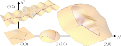
Figure 3: Inverse design of multiple shapes. A flat uniaxial sheet with two designable system features, $\lambda_{i}=\exp(\epsilon_{i}\Lambda^{i}),\,i\in\{1,2\}$, is designed to deform into 3 target shapes in response to two stimuli $\Lambda^{1}$ and $\Lambda^{2}$. A sphere and face-like mask in response to $\Lambda^{1}$ and a wavy sheet in response to $\Lambda^{2}$. The maximal strains are below 300% and are within experimental reach Finkelmann et al. (2001).

Locomotion and work: Cycling between multiple shapes is a standard method of doing work and performing complex tasks. It is of particular importance in microscopic machines, such as swimmers, that, due to their size, operate in settings where viscous forces dominate inertial forces resulting in instantaneous flows that have ‘no memory’. As a consequence only nonreciprocal motions give rise to a net propulsion Purcell (1977). We provide a simple design for a composite sheet that is capable of locomotion in such environments (Fig. 4). The composite sheet consists of two homogeneous layers with independently controllable, orthogonal, director patterns, whose actuated Gaussian curvatures are opposite (Fig. 4a). When the sheets are sequentially actuated and then simultaneously relaxed, they execute a simple non-reciprocal work cycle (Fig. 4b) Mostajeran (2015) that results in an overall translation along the axis of symmetry (Fig. 4c).

This locomotion is powered by the work that the sheet does on its environment. For any actuation, this work is bounded by the frustrated elastic energy Efrati et al. (2009) that would build up if it were constrained to stay in its initial configuration. Because we have defined a common coordinate system we can integrate the energy density along the target surfaces to obtain this bound,

$$\underset{\text{Target Surface}}{E=h\iint\mathcal{E}\left(\lambda_{1},\lambda_{2}\right)}dA,$$ (8)

where $h$ is the sheet’s (unactivated) thickness and the energy density $\mathcal{E}$ on a target surface is derived in the SM SM . Finally, while we have used all the deformation degrees of freedom to obtain the target surfaces, we can still vary the initial conditions to control the sheet’s capacity to do work along a prescribed curve on the target surface. Such control may find applications in the design of lifters Guin et al. (2018b) for instance, where a greater concentration of elastic energy at points of contact may be advantageous. Collectively, the ability to use this inverse design approach to design a sheet that can morph into multiple surfaces capable of executing locomotion and even concentrating elastic energy at specific locations is quite remarkable.

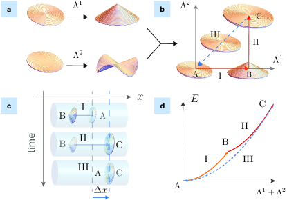
Figure 4: (a) A bilayered uniaxial sheet composed of a top layer with an azimuthal director pattern and a bottom layer with the orthogonal radial director pattern. The top and bottom layers deform into cones and anticones upon actuation, respectively Modes et al. (2010). (b) A nonreciprocal cycle of shape transformations between multiple flat and conical shapes in the bilayered design through the use of two independently controllable stimuli $\Lambda^{1}$ and $\Lambda^{2}$ and the corresponding cycle in parameter space. (c) Locomotion of a swimmer at low Reynolds number with a net displacement $\Delta x$ achieved during each cycle. (d) Bounds on the work, $E$ Eq.(8), that the system can perform on its surroundings at each stage of the cycle.

Discussion. By systematically utilizing multiple degrees of freedom to program a single sheet of material so that it can transform into multiple target geometries, we have provided a vital theoretical foundation for the design of printable sheets capable of executing complex behaviors. The inverse design of a specific system using this approach is straightforward. One needs to: i) specify the set of designable features and how they affect the deformation magnitudes in response to stimuli; ii) select a compatible number of target surfaces to be obtained at specified actuation values; and iii) choose initial conditions for the integration procedure. Using these inputs the code Griniasty (2021) produces designs for the director $\hat{\mathbf{n}}$ and designable features $\bm{\epsilon}$.

Candidate systems for the implementation of this design modality include: (i) Liquid crystal elastomers, where the deformation’s orientation and magnitude can be controlled by varying the nematic director’s in-plane and out-of-plane orientation Ware et al. (2015); Auguste et al. (2018), or the extent of deformation in response to the nematic phase transition Kuenstler et al. (2020). (ii) 4D printed hydrogels, anisotropically deforming along aligned cellulose fibrils, whose orientation in and out of the plane similarly control the deformation’s orientation and magnitude. (iii) Micro robotic kirigami metamaterial sheets where the deformation’s orientation and magnitude can be controlled by varying the local bending of chemical or electrochemical actuators Liu et al. (2021b); Miskin et al. (2020, 2018); Bircan et al. (2020). In each of these examples, the deformations are typically applied globally. As fabrication techniques improve, it may be possible to control the actuation at each point along the surface independently. In this scenario we can use the inverse design framework developed here to obtain the desired target shape by treating the actuation as a designable feature. Such designable local actuations would allow a single sheet to update its target curvatures on the fly and morph into almost any desired surface geometry in real time.

Acknowledgments We thank James Sethna for insightful discussions. This work was supported by the Army Research Office (ARO W911NF-18-1-0032), the National Science Foundation (EFMA-1935252) the Cornell Center for Materials Research (DMR-1719875). I.G. also received partial support from the Cornell Laboratory of Atomic and Solid State Physics. C.M. was supported by Fitzwilliam College and a Henslow Research Fellowship from the Cambridge Philosophical Society.

I Integrating the Inverse design of a uniaxial sheet deforming into $N\geq 2$ surfaces

Let us collect the evolution equations derived in the body of the text with respect to the material coordinates $(u,v)$. The position $\mathbf{r}_{{\bm{\Lambda}}}$ on the different surfaces evolves with the material coordinates according to

$$\partial_{u}\mathbf{r}_{{\bm{\Lambda}}_{i}} =\alpha\lambda_{1}{\hat{\mathbf{n}}_{{\bm{\Lambda}}_{i}}},\quad\partial_{v}\mathbf{r}_{{\bm{\Lambda}}_{i}}=\beta\lambda_{2}\hat{\mathbf{n}}_{{\bm{\Lambda}}_{i}\perp}$$ (S1)

The images of the director on the different surfaces evolves with the material coordinates according to $\kappa_{gu}\hat{\mathbf{n}}_{\perp}=\hat{\mathbf{n}}\cdot\nabla\hat{\mathbf{n}},\,\kappa_{gv}\hat{\mathbf{n}}_{\perp}=\hat{\mathbf{n}}_{\perp}\cdot\nabla\hat{\mathbf{n}}$. Recalling $\nabla_{j{\bm{\Lambda}}}n^{i}_{\bm{\Lambda}}=\partial_{j}n^{i}_{\bm{\Lambda}}+\Gamma^{i}_{{\bm{\Lambda}}jk}n^{k}_{\bm{\Lambda}}$, with $\Gamma_{{\bm{\Lambda}}\,jk}^{i}$ the Levi-Civita connection of the relevant surface, we can write

$$\partial_{u}\hat{\mathbf{n}}_{{\bm{\Lambda}}} ={\alpha\lambda_{1}({\bm{\Lambda}})}\left(\kappa_{gu}({\bm{\Lambda}})\hat{\mathbf{n}}_{{\bm{\Lambda}}\perp}-\hat{\mathbf{n}}_{{\bm{\Lambda}}}\cdot\Gamma_{{\bm{\Lambda}}}\cdot\hat{\mathbf{n}}_{{\bm{\Lambda}}}\right)$$ (S2)

$$\partial_{v}\hat{\mathbf{n}}_{{\bm{\Lambda}}} ={\beta\lambda_{2}({\bm{\Lambda}})}\left(\kappa_{gv}({\bm{\Lambda}})\hat{\mathbf{n}}_{{\bm{\Lambda}}\perp}-\hat{\mathbf{n}}_{{\bm{\Lambda}}\perp}\cdot\Gamma_{{\bm{\Lambda}}}\cdot\hat{\mathbf{n}}_{{\bm{\Lambda}}}\right)$$

The geodesic curvatures of $u$ and $v$ curves are given by

$$\kappa_{gu}=\frac{-\partial_{v}\log(\alpha\lambda_{1})}{\beta\lambda_{2}}=\frac{b}{\lambda_{2}}-\frac{\partial\lambda_{1}}{\lambda_{1}\partial\epsilon}\frac{q}{\lambda_{2}},$$ (S3)

$$\kappa_{gv}=\frac{-\partial_{u}\log(\beta\lambda_{2})}{\alpha\lambda_{1}}=\frac{s}{\lambda_{1}}+\frac{\partial\lambda_{2}}{\lambda_{2}\partial\epsilon}\frac{p}{\lambda_{1}},$$

where

$$b=-\frac{\partial_{v}\alpha}{\alpha\beta},\quad s=\frac{\partial_{u}\beta}{\alpha\beta},\quad\mathbf{p}=\frac{\partial_{u}\bm{\epsilon}}{\alpha}\text{ and }\mathbf{q}=\frac{\partial_{v}\bm{\epsilon}}{\beta}.$$

We reinterpret $b,s,\mathbf{p}$ and $\mathbf{q}$ as propagations of the designable system properties:

$$\partial_{v}\alpha =-\alpha\beta b,$$ (S4)

$$\partial_{u}\beta =\alpha\beta s,$$

$${\partial_{u}\bm{\epsilon}} ={\alpha}\mathbf{p}\text{ and }$$

$${\partial_{v}\bm{\epsilon}} =\beta\mathbf{q}.$$

Finally, to find propagation equations for $b,s,\mathbf{p}$ or $\mathbf{q}$ we cast the Gaussian curvatures as a function of their derivatives:

$$K =\frac{1}{\lambda_{2}^{2}\beta}\partial_{v}b-\frac{1}{\lambda_{1}^{2}\alpha}\frac{\partial\log\lambda_{2}}{\partial\epsilon_{i}}\partial_{u}p_{i}-\frac{1}{\lambda_{2}^{2}\beta}\frac{\partial\log\lambda_{1}}{\partial\epsilon_{i}}\partial_{v}q_{i}-\frac{1}{\lambda_{1}^{2}\alpha}\partial_{u}s$$ (S5)

$$-\frac{b^{2}}{\lambda_{2}^{2}}-\frac{s^{2}}{\lambda_{1}^{2}}-\frac{1}{\lambda_{2}\lambda_{1}}\frac{\partial}{\partial\epsilon_{i}}\left(\frac{1}{\lambda_{1}}\frac{\partial\lambda_{2}}{\partial\epsilon_{j}}\right)p_{i}p_{j}-\frac{1}{\lambda_{2}\lambda_{1}}\frac{\partial}{\partial\epsilon_{i}}\left(\frac{1}{\lambda_{2}}\frac{\partial\lambda_{1}}{\partial\epsilon_{j}}\right)q_{i}q_{j}+\frac{\partial\log(\lambda_{1}^{2}/\lambda_{2})}{\lambda_{2}^{2}\partial\epsilon_{i}}bq_{i}+\frac{\partial\log(\lambda_{1}/\lambda_{2}^{2})}{\lambda_{1}^{2}\partial\epsilon_{i}}sp_{i},$$

where we have assumed Einstein’s summation convention. Extracting the relevant highest order terms

$$\mathbf{d} =\begin{pmatrix}\frac{1}{\beta}\partial_{v}b&\frac{1}{\alpha}\partial_{u}s&dw_{1}&\ldots&dw_{N}\end{pmatrix},$$

$$dw_{i} =\begin{cases}\frac{1}{\alpha}\partial_{u}p_{i}&\text{ if }\exists j\text{ s.t }\partial\lambda_{2}({\bm{\Lambda}}_{j})/\partial\epsilon_{i}\neq 0\\ \frac{1}{\beta}\partial_{v}q_{i}&\text{ else }\end{cases},$$

we define the coefficients matrix

$$M_{i}({\bm{\Lambda}}_{i}) =\begin{pmatrix}\frac{1}{\lambda_{2}^{2}},&-\frac{1}{\lambda_{1}^{2}},&-\frac{1}{\lambda_{1}\lambda_{2}}\frac{\partial\lambda}{\bar{\lambda}\partial\epsilon_{1}},&\ldots,&\frac{1}{\lambda_{1}\lambda_{2}}\frac{\partial\lambda}{\bar{\lambda}\partial\epsilon_{N}}\end{pmatrix},\quad i\in\{1,\ldots,N+2\}$$ (S6)

$$\frac{\partial\lambda}{\bar{\lambda}\partial\epsilon_{i}} =\begin{cases}\frac{\partial\lambda_{2}}{\lambda_{1}\partial\epsilon_{i}}&\text{ if }\exists j\text{ s.t }\partial\lambda_{2}({\bm{\Lambda}}_{j})/\partial\epsilon_{i}\neq 0\\ \frac{\partial\lambda_{1}}{\lambda_{2}\partial\epsilon_{i}}&\text{ else }\end{cases}$$

such that $\bar{\mathbf{K}}=\mathbf{K}-\mathbf{M}\cdot\mathbf{d}$ is independent of ${\mathbf{d}}$, and the inverse design equations of $b,s$ and ${\mathbf{p}}$ or ${\mathbf{q}}$ are given by

$${\mathbf{d}}={\mathbf{M}}^{-1}\cdot({\mathbf{K}}-\bar{\mathbf{K}}).$$ (S7)

I.1 Integrability

The system of equations includes equations along both coordinates $u$ and $v$ for $\mathbf{r},\hat{\mathbf{n}}$ and $\bm{\epsilon}$. The equations are commensurate, $\partial_{u}\partial_{v}\mathbf{r}=\partial_{v}\partial_{u}\mathbf{r}$, and $\partial_{u}\partial_{v}\hat{\mathbf{n}}=\partial_{v}\partial_{u}\hat{\mathbf{n}}$, as has been shown in Griniasty et al. (2019). To show the integrability of the variations of $\bm{\epsilon}$ given in Eq. (S3), consider

$$\partial_{u}\partial_{v}\bm{\epsilon} =\partial_{u}(\beta{\mathbf{q}})=\alpha\beta s{\mathbf{q}}+\beta\partial_{u}{\mathbf{q}},$$

$$\partial_{v}\partial_{u}\bm{\epsilon} =\partial_{v}(\alpha{\mathbf{p}})=-\alpha\beta b{\mathbf{p}}+\alpha\partial_{v}{\mathbf{p}},$$

from which we derive an equation on the initial condition that is preserved through the propagation along $u$ or $v$:

$$\frac{1}{\alpha}\partial_{u}{\mathbf{q}}-\frac{1}{\beta}\partial_{v}{\mathbf{p}}=b{\mathbf{p}}+s{\mathbf{q}}.$$ (S8)

We can then reduce the set of equations by looking at the difference in the propagation of $\mathbf{r},\hat{\mathbf{n}}$ and $\bm{\epsilon}$ along $u$ and along $v$. Changing coordinates to $x_{0}=u-v$, and $x_{1}=u+v$, the system of equations, and analytical initial conditions given along a curve, satisfy the conditions of the Cauchy-Kovalevskaya theorem Kov . Thus, the system is integrable and a solution may be found within a local environment of the initial curve.

Let us complete this section by noting that finding $\partial_{v}{\mathbf{q}}$ of $\partial_{u}{\mathbf{p}}$ (or the inverse) is compatible with a Cauchy problem. A Cauchy initial condition includes $\bm{\epsilon}$ on a non-characteristic curve $\mathbf{r}(l)$ and its derivative across the curve $\partial_{l_{\perp}}\bm{\epsilon}$, as well as the arc-lengths $\alpha$ and $\beta$. The equations $\partial_{l}\partial_{l_{\perp}}\bm{\epsilon}=a_{1}(l)$ and $\partial_{l}\partial_{l}\bm{\epsilon}=a_{2}(l)$ are two linear equations in $\partial_{u}{\mathbf{p}},\,\partial_{v}{\mathbf{p}},\partial_{u}{\mathbf{q}}$ and $\partial_{v}{\mathbf{q}}$, which together with Eq. (S8) can be used to find an equation for $\partial_{v}{\mathbf{q}}(\partial_{u}{\mathbf{p}})$.

I.2 Integrating the system of PDEs

Initial conditions: We show here how to integrate a Goursat-like problem, where the initial conditions are the same as those specified in the main text except for the assignment of initial values of $\bm{\epsilon}$ and their derivatives.

The initial conditions consist of: initial positions and directors on both initial and target surfaces, two perpendicular twice differentiable curves on the initial surface emanating from the initial position, assigned respectively as the initial $u$ and $v$ curves. On the $u$-curve we give $\alpha(u,0)$, and on the $v$-curve $\beta(0,v)$. Finally, for designable features denoted $\epsilon_{i}^{(v)}$, where $dw_{i}=\frac{1}{\alpha}\partial_{u}p$, the initial values $\epsilon_{i}^{(v)}$ and $p_{i}^{(v)}$ are assigned along the initial $v$-curve, while for designable features denoted $\epsilon_{i}^{(u)}$, where $dw_{i}=\frac{1}{\beta}\partial_{v}q$, initial values for $\epsilon_{i}^{(u)}$ and $q_{i}^{(u)}$ are assigned along the initial $u$-curve.

Initialization: The initial data does not explicitly specify the values of all the defined variables appearing in the system of equations that describe the inverse problem. These are $\mathbf{r}_{\bm{\Lambda}},\hat{\mathbf{n}}_{\bm{\Lambda}},\alpha,\beta,\bm{\epsilon},b,s,{\mathbf{p}},{\mathbf{q}}$. To complete the data we need to find $b,s$ and the ${\mathbf{p}},{\mathbf{q}}$ when not prescribed.

For designable features $\epsilon_{i}$ given on the initial $u$-curve ($v$-curve), their variation, and the value of $\alpha$ ($\beta$) along the curve complete the missing data for $p_{i}$ ($q_{i}$). The bend and splay are respectively the geodesic curvatures of the initial $u$ and $v$ curves given by Eq. (S3). Thus, there is complete data at $(u,v)=(0,0)$.

Data propagation: It is convenient to propagate the data along diagonals in the $(u,v)$-plane, as such propagation preserves the $u$-$v$ symmetry of the equations. We implement this approach in the following integration scheme.

The data is divided into sets propagating along $u$ and $v$. $u$-data$=\{\alpha,b,{\mathbf{q}}^{(u)}\}$ propagate along $v$, $v$-data$=\{\beta,s,{\mathbf{p}}^{(v)}\}$ propagate along $u$, $\mathbf{r}_{\bm{\Lambda}},\hat{\mathbf{n}}_{\bm{\Lambda}}$ and $\epsilon$ propagate along both. Given complete data along a diagonal (such as the origin), $u$-data is propagated a step $dv$, $v$-data is propagated a step $du$, and $\mathbf{r}_{\bm{\Lambda}},\hat{\mathbf{n}}_{\bm{\Lambda}}$ and $\epsilon$ are propagated along either. The intersections of the diagonal with the $u$ and $v$ curves contain the missing $u$ and $v$ data. Finally, we complete the data on the new diagonal by propagating $\bm{\epsilon}$ onto the next diagonal to derive ${\mathbf{p}}^{(u)}$ and ${\mathbf{q}}^{(v)}$.

This integration scheme is implemented to inverse design the sheet presented in Fig. S1 which is the same as Figure 3 of the main text. Fig. S1 illustrates the diagonal boundaries in $(u,v)$ whose image we see in the top view of the actuated sheet. Singularities in the integration lead to defects which propagate along the diagonals.

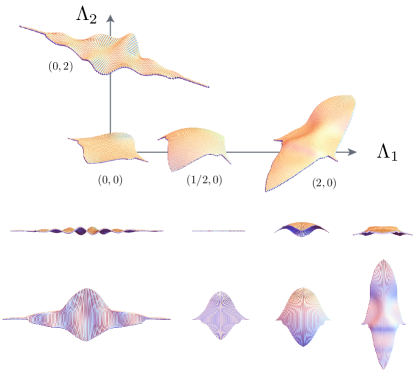
Figure S1: Inverse design of multiple shapes. A flat uniaxial sheet with two designable system features, $\lambda_{i}=\exp(\epsilon_{i}\Lambda^{i}),\,i\in\{1,2\}$, is designed to deform into 3 target shapes in response to two stimuli $\Lambda^{1}$ and $\Lambda^{2}$. A sphere and face-like mask in response to $\Lambda^{1}$ and a wavy sheet in response to $\Lambda^{2}$. Top: Perspective view of the actuated sheet, shown along the stimuli axes. Middle: Front view, demonstrating the variations of the geometries along the $z$ axis. Bottom: Top view, demonstrating the mapping of the boundaries, and their underlying diagonal structure in the $u,v$ coordinates.

I.3 A word of caution on the choice of actuation sets

The four-surface inverse problem is set up by attributing a pair of values to the actuation parameters $\{(\Lambda_{1}^{(i)},\Lambda_{2}^{(i)})\}_{i=0}^{3}$ for each of the surfaces. Surprisingly, some sets of actuation pairs systematically do not lead to an integrable set of PDEs for $\{\alpha,\beta,\epsilon_{1},\epsilon_{2}\}$. This is captured by $\mathrm{det}({\mathbf{M}})=0$, that is, a linear dependence of the target curvatures via $\bar{\mathbf{K}}$ on the highest order derivatives ${\mathbf{d}}$. One such example is $(\lambda_{1},\lambda_{2},K)\in\{(0,0,K_{0}),(\Omega_{1},0,K_{1}),\,(\Omega_{1},\Omega_{2},K_{2}),\,(0,\Omega_{2},K_{3})\}$. The induced system of equations are 3 independent PDEs of second order in $\alpha,\beta,\epsilon_{1}$ and $\epsilon_{2}$ given the curvatures $\{K_{0},K_{1},K_{2}\}$ and a first order PDE given all four curvatures, composing a system of PDEs with a constraint whose solution is beyond the scope of this paper. We note that the manifold of actuation pairs with vanishing determinants is of co-dimension $1$, and so, rare.

Elastic energy calculations in frustrated uniaxial systems

The total elastic energy in the reduced 2D model of non-Euclidean elasticity theory Efrati et al. (2009) takes the form

$$E=hE_{S}+h^{3}E_{B},$$ (S9)

where $h$ is the thickness of the sheet and

$$E_{S}=\int w_{S}\sqrt{|\bar{g}|}dx^{1}dx^{2},\quad\quad\quad E_{B}=\int w_{B}\sqrt{|\bar{g}|}dx^{1}dx^{2}$$ (S10)

are the stretching and bending contents of the energy determined by

$$w_{S} =\frac{Y}{8(1+\nu_{e})}\left(\frac{\nu_{e}}{1-\nu_{e}}\bar{g}^{ij}\bar{g}^{kl}+\bar{g}^{ik}\bar{g}^{jl}\right)(g_{ij}-\bar{g}_{ij})(g_{kl}-\bar{g}_{kl})$$ (S11)

$$w_{B} =\frac{Y}{24(1+\nu_{e})}\left(\frac{\nu_{e}}{1-\nu_{e}}\bar{g}^{ij}\bar{g}^{kl}+\bar{g}^{ik}\bar{g}^{jl}\right)b_{ij}b_{kl}.$$ (S12)

Here $\bar{g}$ denotes the 2D reference metric (i.e. the metric of the target surface) and $g$ the actual metric. Integration in Eq. (S10) is with respect to the reference metric and the indices run over $1$ and $2$ using Einstein notation. $b$ denotes the second fundamental form of the realized surface. $Y$ denotes the Young’s modulus and $\nu_{e}$ the Poisson ratio of the material.

For thin sheets, the bending contribution of the energy is dominated by the stretching contribution as $h^{3}\approx 0$. In the thin sheet limit, the actual metric will match the reference metric of the target surface in the unconstrained problem so that the stretching contribution becomes zero and the final configuration is determined by an isometric embedding of the metric that minimizes the bending energy. On the other hand, if the system is constrained (i.e. stretching is blocked somehow), the stretching energy will quickly build up as the actual metric is prevented from matching the reference metric and the bending energy will be negligible in comparison. This stretching energy will then provide an upper bound on the amount of energy that can be extracted from the activation of such a surface to do work, e.g. as lifters Guin et al. (2018).

Considering only the stretching contribution to the elastic energy of a constrained activated surface, we can express the elastic energy as

$$E=\frac{hY}{8(1-\nu_{e}^{2})}\int\left[(1-\nu_{e})\operatorname{Tr}\left(\bar{g}^{-1}(g-\bar{g})\right)^{2}+\nu_{e}\operatorname{Tr}^{2}\left(\bar{g}^{-1}(g-\bar{g})\right)\right]\sqrt{|\bar{g}|}dx^{1}dx^{2},$$ (S13)

using the trace operator $\operatorname{Tr}$. Working in the $(u,v)$-coordinate system outlined in the paper, the pre-actuated metric takes the form $ds^{2}=\alpha^{2}du^{2}+\beta^{2}dv^{2}$ and the activated (reference) metric becomes $ds^{2}_{A}=\lambda_{1}({\bm{\Lambda}},\bm{\epsilon})^{2}\alpha^{2}du^{2}+\lambda_{2}({\bm{\Lambda}},\bm{\epsilon})^{2}\beta^{2}dv^{2}$, where $\lambda_{1}$ and $\lambda_{2}$ can in general depend on $(u,v)$ through the designable material features $\bm{\epsilon}=\bm{\epsilon}(u,v)$. If the activated sheet is blocked from deforming, we have

$$g=\begin{pmatrix}\alpha(u,v)^{2}&0\\ 0&\beta(u,v)^{2}\end{pmatrix},\quad\bar{g}=\begin{pmatrix}\lambda_{1}(u,v)^{2}\alpha(u,v)^{2}&0\\ 0&\lambda_{2}(u,v)^{2}\beta(u,v)^{2}\end{pmatrix}.$$ (S14)

Substituting into Eq. (S13), we obtain

$$E=h\underset{\text{Target Surface}}{\iint}\mathcal{E}(\lambda_{1},\lambda_{2})dA,$$ (S15)

where

$$\mathcal{E}(\lambda_{1},\lambda_{2})=\frac{Y}{8(1-\nu_{e}^{2})}\left[(1-\nu_{e})\left(\left(1-\frac{1}{\lambda_{1}^{2}}\right)^{2}+\left(1-\frac{1}{\lambda_{2}^{2}}\right)^{2}\right)+\nu_{e}\left(\frac{1}{\lambda_{1}^{2}}+\frac{1}{\lambda_{2}^{2}}-2\right)^{2}\right],$$ (S16)

and $dA=\lambda_{1}\lambda_{2}\alpha\beta dudv$ is the area measure on the target surface.

As an illustrative example, we consider the case of a baromorph with $\lambda_{1}=1$ and $\lambda_{2}=1+\Lambda\epsilon$, where $\Lambda$ denotes pressure and $\epsilon$ is a designable feature related to the channel thickness Siéfert et al. (2019). Substituting into Eq. (S15), we obtain

$$E=\frac{hY}{8(1-\nu_{e}^{2})}\int\frac{\epsilon^{2}\Lambda^{2}(2+\Lambda\epsilon)^{2}}{(1+\Lambda\epsilon)^{3}}\alpha\beta dudv.$$ (S17)

If the baromorph is homogeneous so that $\epsilon$ is constant, the elastic energy takes the simplified form

$$E=\frac{hA_{0}Y}{8(1-\nu_{e}^{2})}\frac{\epsilon^{2}\Lambda^{2}(2+\Lambda\epsilon)^{2}}{(1+\Lambda\epsilon)^{3}},$$ (S18)

where $A_{0}$ is the area of the unactuated sheet.

In the main text, we consider a system with two degrees of freedom in actuation whose metric is given by

$$ds^{2}=(1+\Lambda_{2}\epsilon)^{2}v^{2}du^{2}+(1+\Lambda_{1}\epsilon)^{2}dv^{2},$$ (S19)

where $\epsilon$ is taken to be a constant. As depicted in Figure 4 (d) of the main text, a 3-stage cycle is executed by taking $(\Lambda_{1},\Lambda_{2})=(0,0)\rightarrow(1,0)\rightarrow(1,1)\rightarrow(0,0)$ along straight lines in parameter space. The elastic energy in the frustrated system in stage I is simply Eq. (S18) with $\Lambda=\Lambda_{1}$. In stage II, the elastic energy can be calculated by taking the reference metric as $ds^{2}=(1+\Lambda_{2}\epsilon)^{2}v^{2}du^{2}+(1+\epsilon)^{2}dv^{2}$ and varying $\Lambda_{2}$ from 0 to 1. Finally, the elastic energy in stage III is found by taking the reference metric to be $ds^{2}=(1+\Lambda\epsilon)^{2}v^{2}du^{2}+(1+\Lambda\epsilon)^{2}dv^{2}$ where $\Lambda=\Lambda_{1}=\Lambda_{2}$, which yields

$$E=\frac{hA_{0}Y}{4(1-\nu_{e})}\frac{\epsilon^{2}\Lambda^{2}(2+\Lambda\epsilon)^{2}}{(1+\Lambda\epsilon)^{2}}.$$ (S20)

These energy calculations are combined to produce the plot in Figure 4 (d) of the main text, which further demonstrates the non-reciprocal nature of the cycle.

Finally, we note that while the non-Euclidean plate theory used above is valid for large displacements but small strains, it can be extended to systems involving large strains using suitable hyperelastic models, such as Mooney-Rivlin or neo-Hookean models. For instance, the corresponding stretching energy for a thin membrane of incompressible neo-Hookean elastomer takes the form

$$E=h\underset{\text{Target Surface}}{\iint}\frac{Y}{4(1+\nu_{e})}\left[\operatorname{Tr}\left(\bar{g}^{-1}g\right)+\frac{1}{\det\left(\bar{g}^{-1}g\right)}-3\right]\frac{dA}{\lambda_{1}\lambda_{2}}$$ (S21)

and can be used to describe elastomers experiencing large strain deformations Duffy and Biggins (2020). Repeating the earlier analysis with this stretch energy, $\mathcal{E}$ is replaced by

$$\mathcal{E}(\lambda_{1},\lambda_{2})=\frac{Y}{4(1+\nu_{e})}\left(\frac{1}{\lambda_{1}^{2}}+\frac{1}{\lambda_{2}^{2}}+\lambda_{1}^{2}\lambda_{2}^{2}-3\right)\frac{1}{\lambda_{1}\lambda_{2}},$$ (S22)

which agrees with Eq. (S16) for small strains to quadratic order.

References

- Miskin et al. (2020) M. Z. Miskin, A. J. Cortese, K. Dorsey, E. P. Esposito, M. F. Reynolds, Q. Liu, M. Cao, D. A. Muller, P. L. McEuen, and I. Cohen, Nature 584, 557 (2020).
- Reyssat and Mahadevan (2009) E. Reyssat and L. Mahadevan, Journal of the Royal Society, Interface 6, 951 (2009).
- Wallin et al. (2018) T. J. Wallin, J. Pikul, and R. F. Shepherd, Nature Reviews Materials 3, 84 (2018).
- Teo et al. (2016) A. J. T. Teo, A. Mishra, I. Park, Y.-J. Kim, W.-T. Park, and Y.-J. Yoon, ACS Biomaterials Science & Engineering, ACS Biomaterials Science & Engineering 2, 454 (2016).
- Hartl and Lagoudas (2007) D. J. Hartl and D. C. Lagoudas, Proceedings of the Institution of Mechanical Engineers, Part G: Journal of Aerospace Engineering 221, 535 (2007).
- Guin et al. (2018a) T. Guin, M. J. Settle, B. A. Kowalski, A. D. Auguste, R. V. Beblo, G. W. Reich, and T. J. White, Nature Communications 9, 2531 (2018a).
- Palagi and Fischer (2018) S. Palagi and P. Fischer, Nature Reviews Materials 3, 113 (2018).
- Levin et al. (2020) I. Levin, R. Deegan, and E. Sharon, Phys. Rev. Lett. 125, 178001 (2020).
- Demaine and Tachi (2017) E. D. Demaine and T. Tachi, in 33rd International Symposium on Computational Geometry (SoCG 2017) (Schloss Dagstuhl-Leibniz-Zentrum fuer Informatik, 2017).
- Na et al. (2015) J.-H. Na, A. A. Evans, J. Bae, M. C. Chiappelli, C. D. Santangelo, R. J. Lang, T. C. Hull, and R. C. Hayward, Advanced Materials 27, 79 (2015).
- Liu et al. (2021a) Q. Liu, W. Wang, M. F. Reynolds, M. C. Cao, M. Z. Miskin, T. A. Arias, D. A. Muller, P. L. McEuen, and I. Cohen, Science Robotics 6 (2021a).
- Manna et al. (2020) R. K. Manna, O. E. Shklyaev, H. A. Stone, and A. C. Balazs, Mater. Horiz. 7, 2314 (2020).
- Modes and Warner (2016) C. Modes and M. Warner, Physics today 69, 32 (2016).
- Korn (1914) A. Korn, “Zwei anwendungen der methode der sukzessiven annäherungen,” in Mathematische Abhandlungen Hermann Amandus Schwarz, edited by C. Carathéodory, G. Hessenberg, E. Landau, and L. Lichtenstein (Springer Berlin Heidelberg, Berlin, Heidelberg, 1914) pp. 215–229.
- Lichtenstein (1916) L. Lichtenstein, Zur theorie der konformen abbildung: Konforme abbildung nichtanalytischer, singularitätenfreier flächenstücke auf ebene gebiete (Verlag nicht ermittelbar, 1916).
- Kim et al. (2012a) J. Kim, J. A. Hanna, M. Byun, C. D. Santangelo, and R. C. Hayward, Science 335, 1201 (2012a).
- Pikul et al. (2017) J. H. Pikul, S. Li, H. Bai, R. T. Hanlon, I. Cohen, and R. F. Shepherd, Science 358, 210 (2017).
- Kim et al. (2012b) J. Kim, J. A. Hanna, R. C. Hayward, and C. D. Santangelo, Soft Matter 8, 2375 (2012b).
- Klein et al. (2007) Y. Klein, E. Efrati, and E. Sharon, Science 315, 1116 (2007).
- Griniasty et al. (2019) I. Griniasty, H. Aharoni, and E. Efrati, Phys. Rev. Lett. 123, 127801 (2019).
- Fahn and Zohary (1955) A. Fahn and M. Zohary, Phytomorph. 5, 99 (1955).
- Armon et al. (2011) S. Armon, E. Efrati, R. Kupferman, and E. Sharon, Science 333, 1726 (2011).
- Aharoni et al. (2012) H. Aharoni, Y. Abraham, R. Elbaum, E. Sharon, and R. Kupferman, Physical Review Letters 108, 238106 (2012).
- Aharoni et al. (2014) H. Aharoni, E. Sharon, and R. Kupferman, Phys. Rev. Lett. 113, 257801 (2014).
- Mostajeran (2015) C. Mostajeran, Physical Review E - Statistical, Nonlinear, and Soft Matter Physics 91 (2015).
- Sydney Gladman et al. (2016) A. Sydney Gladman, E. A. Matsumoto, R. G. Nuzzo, L. Mahadevan, and J. A. Lewis, Nature Materials 15, 413 EP (2016).
- Ware et al. (2015) T. H. Ware, M. E. McConney, J. J. Wie, V. P. Tondiglia, and T. J. White, Science 347, 982 (2015).
- Mostajeran et al. (2016) C. Mostajeran, M. Warner, T. H. Ware, and T. J. White, Proceedings of the Royal Society of London A: Mathematical, Physical and Engineering Sciences 472 (2016).
- Aharoni et al. (2018) H. Aharoni, Y. Xia, X. Zhang, R. D. Kamien, and S. Yang, Proc. Nat. Aca. Sci 115, 7206 (2018).
- Warner and Mostajeran (2018) M. Warner and C. Mostajeran, Proc. R. Soc. A 474, 20170566 (2018).
- Kowalski et al. (2018) B. A. Kowalski, C. Mostajeran, N. P. Godman, M. Warner, and T. J. White, Phys. Rev. E 97, 012504 (2018).
- Siéfert and Warner (2020) E. Siéfert and M. Warner, Proc. R. Soc. A. (2020).
- Duffy and Biggins (2020) D. Duffy and J. S. Biggins, Soft Matter 16, 10935 (2020).
- Feng et al. (2020) F. Feng, J. S. Biggins, and M. Warner, Phys. Rev. E 102, 013003 (2020).
- Siéfert et al. (2019) E. Siéfert, E. Reyssat, J. Bico, and B. Roman, Nature Materials 18, 24 (2019).
- Giudici and Biggins (2021) A. Giudici and J. S. Biggins, Journal of Applied Physics 129, 154701 (2021).
- Niv and Efrati (2018) I. Niv and E. Efrati, Soft Matter 14, 424 (2018).
- (38) See Supplemental Material for additional information on the integration scheme and the elastic energy density.
- Note (1) By definition, is a designable elastic feature so that either or . Without loss of generality we take . Otherwise, and by exchanging the director with , we rename as . Further, it is sufficient that only for one value of the actuation , .
- Hadamard (1923) J. Hadamard, Lectures on Cauchy’s problem in linear partial differential equations (Yale University press, 1923).
- Evans (2010) L. C. Evans, Partial Differential Equations (Graduate Studies in Mathematics, Vol. 19), 2nd ed. (American Mathematical Society, 2010).
- Press et al. (2007) W. H. Press, S. A. Teukolsky, W. T. Vettering, and B. P. Flannery, NUMERICAL RECIPES The Art of Scientific Computing Third Edition (2007).
- Goursat (1923) E. Goursat, Cours d’analyse mathématique, Vol. 3 (Gauthier-Villars, 1923).
- Finkelmann et al. (2001) H. Finkelmann, E. Nishikawa, G. G. Pereira, and M. Warner, Phys. Rev. Lett. 87, 015501 (2001).
- Purcell (1977) E. M. Purcell, American Journal of Physics 45, 3 (1977).
- Efrati et al. (2009) E. Efrati, E. Sharon, and R. Kupferman, Journal of the Mechanics and Physics of Solids 57, 762 (2009).
- Guin et al. (2018b) T. Guin, M. J. Settle, B. A. Kowalski, A. D. Auguste, R. V. Beblo, G. W. Reich, and T. J. White, Nature Communications 9, 2531 (2018b).
- Modes et al. (2010) C. D. Modes, K. Bhattacharya, and M. Warner, Proceedings of the Royal Society A: Mathematical, Physical and Engineering Sciences 467, 1121 (2010).
- Griniasty (2021) I. Griniasty, “Multi-surface inverse design: Calculating the designable properties of a uniaxial sheet,” (2021).
- Auguste et al. (2018) A. D. Auguste, J. W. Ward, J. O. Hardin, B. A. Kowalski, T. C. Guin, J. D. Berrigan, and T. J. White, Advanced Materials 30, 1802438 (2018).
- Kuenstler et al. (2020) A. S. Kuenstler, Y. Chen, P. Bui, H. Kim, A. DeSimone, L. Jin, and R. C. Hayward, Advanced Materials 32, 2000609 (2020).
- Liu et al. (2021b) Q. Liu, W. Wang, H. Sinhmar, A. Cortese, I. Griniasty, M. Reynolds, M. Taghavi, A. Apsel, H. Kress-Gazit, P. McEuen, et al., Bulletin of the American Physical Society (2021b).
- Miskin et al. (2018) M. Z. Miskin, K. J. Dorsey, B. Bircan, Y. Han, D. A. Muller, P. L. McEuen, and I. Cohen, Proceedings of the National Academy of Sciences 115, 466 (2018).
- Bircan et al. (2020) B. Bircan, M. Z. Miskin, R. J. Lang, M. C. Cao, K. J. Dorsey, M. G. Salim, W. Wang, D. A. Muller, P. L. McEuen, and I. Cohen, Nano Letters 20, 4850 (2020).
Supplemental material - Multi-valued inverse design: multiple surface geometries from one flat sheet

References

- Griniasty et al. (2019) I. Griniasty, H. Aharoni, and E. Efrati, Phys. Rev. Lett. 123, 127801 (2019).
- (2) Cauchy-Kovalevskaya theorem, Encyclopedia of Mathematics .
- Efrati et al. (2009) E. Efrati, E. Sharon, and R. Kupferman, Journal of the Mechanics and Physics of Solids 57, 762 (2009).
- Guin et al. (2018) T. Guin, M. J. Settle, B. A. Kowalski, A. D. Auguste, R. V. Beblo, G. W. Reich, and T. J. White, Nature Communications 9, 2531 (2018).
- Siéfert et al. (2019) E. Siéfert, E. Reyssat, J. Bico, and B. Roman, Nature Materials 18, 24 (2019).
- Duffy and Biggins (2020) D. Duffy and J. S. Biggins, Soft Matter 16, 10935 (2020).