A Comparison of Deep-Learning Methods for Analysing and Predicting Business Processes

Abstract

Deep-learning models such as Convolutional Neural Networks (CNN) and Long Short-Term Memory (LSTM) have been successfully used for process-mining tasks. They have achieved better performance for different predictive tasks than traditional approaches. We extend the existing body of research by testing four different variants of Graph Neural Networks (GNN) and a fully connected Multi-layer Perceptron (MLP) with dropout for the tasks of predicting the nature and timestamp of the next process activity. In contrast to existing studies, we evaluate our models’ performance at different stages of a process, determined by quartiles of the number of events and normalized quarters of the case duration. This provides new insights into the performance of a prediction model, as they behave differently at different stages of a business-process. Interestingly, our experiments show that the simple MLP often outperforms more sophisticated deep-learning models in both prediction tasks. We argue that care needs to be taken when applying automated process-prediction techniques at different stages of a process. We further argue that researchers should reflect their results with strong baselines methods like MLPs.

I Introduction

Most businesses thrive on the effective use of event logs and process records. The ability to predict the nature of an unseen event in a business-process can have very useful applications [4]. This can help in more efficient customer service, and facilitate in developing an improved work-plan for companies. The domain of process mining deals with combining a wide range of classical model-based predictive techniques along with traditional data-analysis techniques [27]. A process can be a representation of any set of activities that take place in a business enterprise; for example, the procedure for obtaining a financial document, the steps involved in a complaint-registering system, etc.

Business-process mining, in general, deals with the analysis of the sequence of events produced during the execution of such processes [6, 16, 18]. Even though the classical approach of depicting event logs is with the help of process graphs [1, 30], Pasquadibisceglie et al. [20], Tax et al. [23], Taymouri et al. [25], and others have recently applied deep-learning techniques like Convolutional Neural Networks (CNN), Long Short-Term Memory (LSTM) networks, and Generative Adversarial Nets (GANs) for the task of predictive process mining. The deep-learning based models obtained results that outperformed traditional models.

Inspired from these works and taking into consideration the graph nature of processes, we aim to model event logs as graph structures and apply different Graph Neural Network (GNN) models on such data structures. GNNs have shown superior results for the vertex-classification task  [14], link-prediction task [33], and recommender systems [32]. In this work, we use a new representation for the event-log data and investigated the performance of different variants of a Graph Convolutional Network (GCN) [14] as a successful example of GNNs. We compare the GCN model among others with the CNN and LSTM models along with a Multi-Layer Perceptron (MLP) and classical process-mining techniques [4, 28].

In contrast to the existing body of research [20, 9, 5, 23, 25, 15], we analyze how the performance of the models for business-process prediction depend on the stage of a process. The results show that the next activity type and timestamp prediction depend a lot on the model and also on whether an early, mid, or late stage of the process is considered. Furthermore, we observe from our experiments that MLP is a strong baseline and in many cases outperforms more advanced neural networks like LSTMs, GCNs, and CNNs. The MLP model achieves a maximum of 82% accuracy in predicting the next event type, and a minimum mean absolute error of 1.3229 days for predicting the timestamp of the next event.

Below, we discuss related works in business-process mining. Section III introduces our experimental apparatus, datasets and pre-processing, as well as our GCN-based models. Sections IV and  V highlights the major results from the experiments, followed by a discussion in Section VI, before we conclude.

II Related Works

Business-process mining deals with several prediction tasks like predicting the next activity type [2, 23, 20, 9, 4], the timestamp of the next event in the process [23, 28], the overall outcome of a given process [24], or the time remaining until the completion of a given process instance [21]. There is a huge body of algorithms for these process-mining tasks [4, 28]. In the context of this work, we focus on the first two aspects of the aforementioned list of predictive tasks, namely, the task of predicting the nature and timestamp of the next event in a given process. We reconsider the results from the classical methods and compare them with latest developments on business-process mining using deep learning.

There has been a recent shift towards deep-learning models for the task of predictive business-process monitoring. Tax et al. [23] proposed to use a Recurrent Neural Network (RNN) architecture with Long Short-Term Memory (LSTM) for the task of predicting the next activity and timestamp, the remaining cycle time, and the sequence of remaining events in a case. Their model was able to model the temporal properties of the data and improve on the results obtained from traditional process-mining techniques. The main motivation for using an LSTM model was to obtain results that were consistent for a range of tasks and datasets. The LSTM architecture of Tax et al. could also be extended to the task of predicting the case outcome. Camargo et al. [5] and Lin et al. [15] both use LSTM models, too. The first one to predict the next event including timestamp and the associated resource pool, the latter to predict the next event, including its attributes. Evermann et al. [9] also used RNN for the task of predicting the next event on two real-life datasets. Their system architecture involved two hidden RNN layers using basic LSTM cells.

Pasquadibisceglie et al. [20] used Convolutional Neural Networks (CNN) for the task of predictive process analytics. An image-like data engineering approach was used to model the event logs and obtain results from benchmark datasets. In order to adapt a CNN for process-mining tasks, a novel technique of transforming temporal data into a spatial structure similar to images was introduced. The CNN results improve over the accuracy scores obtained by Tax et al.’s LSTM [23] for the task of predicting the next event.

Scarselli et al. [22] introduced Graph Neural Networks (GNNs) as a new deep-learning technique that could efficiently perform feature extraction. Especially in the last year, GNNs have gained widespread attention and use in different domains. Wu et al. [31] provided a comprehensive survey of GNNs. They categorize the different GNN architectures into Graph Convolutional Networks (GCN, or also called: ConvGNN), Spatio-temporal Graph Neural Networks (STGNNs), Recurrent Graph Neural Networks (RecGNN), and Graph Autoencoders (GAEs). Esser et al. [8] discussed the advantages of using graph structures to model event logs. Performing process-mining tasks by modelling the relationships between events and case instances as process graphs has been a widely accepted approach [19, 29].

Recently, Taymouri et al. [25] have used Generative Adversarial Nets (GANs) for predicting the next activity and its timestamp. In a minmax game of discriminator and generator, both consisting of RNNs in a LSTM architecture and feedforward neural networks, a prediction is made of the next step, including event type and event-timestamp prediction. Taymouri et al. used different models each trained over a specific length of sub-sequences of processes, modeled by the parameter $k$. For example, a value of $k=20$ means that sub-sequences of length $20$ are used for training, and testing would be applied on process steps $21$, $22$, $23$, and following until the end of the process.

Other works used features from unstructured data like texts in deep-learning architectures to improve the process-prediction task. Ding et al. [7] demonstrate how a deep-learning model using events extracted from texts improves predictions in the stock markets domain. For business-process modelling, Teinemaa et al. [26] improve the performance of predictive business models by using text-mining techniques on the unstructured data present in event logs.

In this work, we aim to combine traditional process mining from event graphs along with deep-learning techniques like GCNs to achieve a better performance in predictive business-process monitoring. We evaluate each of the model variants at different stages of a process, determined by quartiles of the number of events in a case and normalized quarters computed over the case durations. This would provide a more detailed understanding of the models’ performance.

III Experimental Apparatus

We introduce the datasets used in this work and the methodology adopted for representing the feature vectors corresponding to each row in the dataset. Following this, a mathematical formulation of graphs and the specific case of process graphs is provided, which lays the foundation to understand a Graph Convolutional Network. We conclude with a description of the procedure and metrics adopted for this work.

III-A Datasets

We use two well-known benchmark event-log datasets, namely Helpdesk and BPI12 (W). These two representative datasets have been chosen as they are used by the models we want to compare with, namely the CNN by Pasquadibisceglie et al. [20], LSTMs from Camargo et al. [5] and Tax et al. [23], and the GAN from Taymouri et al. [25]. Thus, the datasets best possible serve the purpose to compare the different Deep-Learning architectures. All datasets are characterised by three columns: “Case ID” (the process-case identifier), “Activity ID” (the event-type identifier), and the “Complete Timestamp” denoting the time at which a particular event took place. Table I shows an overview of the datasets.

Table I: Overview of the datasets used

Attribute	Dataset
	Helpdesk	BPI12(W)
No. of events	13,710	72,413
No. of process cases	3,804	9,658
No. of activity types	9	6
Avg. case duration (sec.)	22,475	1,364
Avg. no. of events per case	3.604	7.498

Helpdesk dataset

This dataset presents event logs obtained at the helpdesk of an Italian software company. The events in the log correspond to the activities associated with different process instances of a ticket management scenario. It is a database of 13,710 events related to 3,804 different process instances. There are 9 activity types, i. e., classes in the dataset. Each process contains events from a list of nine unique activities involved in the process. A typical process instance spans events from inserting a new ticket, until it is closed or resolved. Table I shows the average case duration and the number of activities per case.

BPIC’12 (Sub-process W) dataset

The Business-Process Intelligence Challenge (BPIC’12) dataset contains event logs of a process consisting of three sub-processes, which in itself is a relatively large dataset. As described in [23] and [20], only completed events that are executed manually are taken into consideration for predictive analysis. This dataset, called BPI12 (W), includes 72,413 events from 9,658 process instances. Each event in a process is one among 6 activity types involved in a process instance, i. e., a process case. The activities denote the steps involved in the application procedure for financial needs, like personal loans and overdrafts.

III-B Graphs and Graph Convolutional Layer

A graph can be represented as $G=(V,E)$, where V is the set of vertices and E denotes the edges present between the vertices [31]. An edge between vertex i and vertex j is denoted as e_ij $\in$ E. A graph can be either directed or undirected, depending on the nature of interaction between the vertices. In addition, a graph may be characterized by vertex attributes or edge attributes, which in simple terms are feature vectors associated with that particular vertex or edge. The adjacency matrix of a graph is an $n\times n$ matrix with A_ij = 1 if e_ij $\in$ E and A_ij = 0 if e_ij $\notin$ E, where n is the number of vertices in the graph. A degree matrix is a diagonal matrix which stores the degree of each vertex, which numerically corresponds to the number of edges that the node is attached to.

A GCN layer operates by calculating a hidden embedding vector for each node of the graph. It calculates this hidden vector by combining each node’s feature-vector with the adjacency matrix for the graph, by the equation (Kipf and Welling [14]):

$$f(X,A,W)=\sigma(D^{-1}AXW),$$ (1)

where X is the input-feature matrix containing the feature vector for each of the vertices, A is the adjacency matrix of the graph, D is the degree matrix, W is a learnable weight matrix, and $\sigma$ is the activation function of that layer.

In (1), the product $D^{-1}A$ represents an attempt to normalize the adjacency matrix. However, as matrix multiplication is non-commutative, an alternative symmetric normalisation is preferred [14], changing the GCN layer’s operation to:

$$f(X,A,W)=\sigma(D^{-\frac{1}{2}}AD^{-\frac{1}{2}}XW)$$ (2)

Note, all the models used in this work, the GCN layer calculations are done as described in (2). For the model variants described in Section III-F involving the Laplacian matrix, the adjacency matrix ($A$) in (2) is replaced by the corresponding unnormalized Laplacian.

III-C Data Pre-processing

The timestamp corresponding to each event in the dataset can be used to derive a feature-vector representation for each row in the data. The approach introduced in [23] has been used to initially get a feature vector consisting of the following four elements: 1. The time since previous event in the case. 2. The time since the case started. 3. The time since midnight. 4. The day of the week for the event. All four values are treated as real-valued durations. This results in a 4-element feature vector for every row in the dataset. The drawback in this kind of a representation is that it treats each event in a case independently. In order to overcome this drawback, it was necessary for the feature vector of every event to have a history of other events that had already occurred for that particular Case ID. Hence, a new comprehensive feature vector representation was introduced.

In this work, each entry in a dataset is assigned a matrix representation (X) whose dimensions depend on the dataset which is considered. The number of rows in X can be obtained by identifying the unique entries in the ‘Activity ID’ column, i. e., the unique activity types as shown in Table I, or can be visually identified as the number of vertices in the process graphs for each of the datasets (Figure 1). Let us denote this value by ‘num$\_$of$\_$nodes’ for ease of representation. As it can be observed from Table I, num$\_$of$\_$nodes is 9 for the Helpdesk dataset and 6 for the BPI’12 (W) dataset. The number of columns in X corresponds to the length of the initial feature vector, i. e., 4. This would result in a matrix of size ‘$num\_of\_nodes\times 4$’ for each data entry.

The matrix X is first initialized with zeroes. Each row index of $X$ stores the 4-element long feature vector corresponding to the most-recent Activity ID denoted by that particular row index, for the current case ID. For example, the first row stores the 4-element long feature vector for the event with Activity ID equal to 1, and so on. One approximation that we have used in this step is that if an event corresponding to a particular Activity ID has occurred more than once in a case, we use the feature vector for only the most-recent occurrence of that event. In scenarios where events with a particular Activity ID have not occurred yet in a given case, the feature matrix will hence just store a vector with zeroes corresponding to that Activity ID. This method of representation gives each row of the Helpdesk dataset a $9\times 4$ matrix, and each row of the BPI’12 (W) dataset a $6\times 4$ matrix. The motivation behind choosing such a representation is to facilitate the computation involved in a Graph Convolutional Layer, as explained in Section III-B. For a given row, the Activity ID of the next event and the time since current event are taken as the target labels for the event-predictor and the time-predictor, respectively.

III-D Process Graphs as Input to GCNs

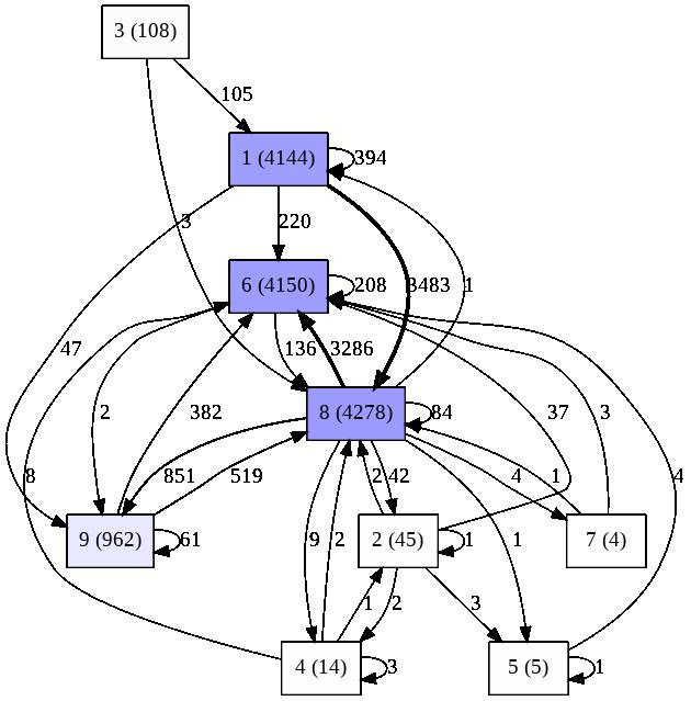
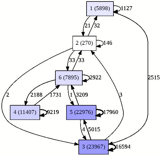
Figure 1: Directly-follows graphs generated for the Helpdesk dataset (left) and BPI’12 (W) dataset (right) using PM4Py. The vertices represent the unique Activity IDs (i. e., activity types) along with their frequencies denoted in brackets. The numbers on the directed edges denote the frequency of directly-follows relations.

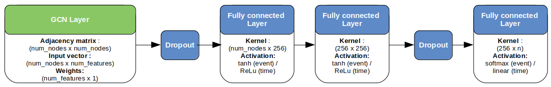
Figure 2: Graph Convolutional Network architecture for the event type and timestamp predictor. The value for n in the last layer denotes the number of classes for the event predictor and 1 for the time predictor.

Process discovery from event logs can be achieved using different traditional process-mining techniques. In this work, we have used an inductive mining approach with Directly-Follows Graphs (DFGs) to represent the processes extracted from each of the datasets. The choice is motivated by the simplicity and efficiency with which the entire data can be represented in the form of a graph.

A Directly-Follows Graph for an Event Log L is denoted as [27]: $G(L)=(A_{L},\mapsto_{L},A_{L}^{start},A_{L}^{end})$, where A_L is the set of activities in L with A${}_{L}^{start}$ and A${}_{L}^{end}$ denoting the set of start and end activities, respectively. $\mapsto_{L}$ denotes the directly-follows operation, which exists between two events if and only if there is a case instance in which the source event is followed by the other target event. The vertices in the graph represent the unique activities present in the event log, and the directed edges of the graph exist if there is a directly-follows relation between the vertices. The number of directly-follows relations that exist between two vertices is denoted by a weight for the corresponding edge.

Berti et al. [3] presented a process-mining tool for Python called PM4Py. The Directly-Follows Graphs for both the datasets (considering all the events/rows) were visualised using the PM4Py package as shown in Figure 1. Consider the following binary adjacency matrix for the process graph generated, as example, from the BPI’12 (W) dataset:

$$B_{BPI^{\prime}12(W)}=\begin{bmatrix}1&1&1&0&0&0\\ 1&1&1&0&0&1\\ 0&1&1&0&1&0\\ 0&0&0&1&0&1\\ 0&0&1&0&1&1\\ 0&1&0&1&1&1\\ \end{bmatrix}$$

This $6\times 6$ matrix needs to be normalized as per Equation (2) to be used in a GCN. The elements of the diagonal degree matrix can be numerically computed as a row-wise sum from the above matrix. The dimensions of the normalized matrix ($6\times 6$) and the dimension of X ($6\times 4$ for BPI’12 (W) dataset) makes it compatible for matrix multiplication in the GCN layer. In general, the normalized adjacency matrix will have dimensions $num\_of\_nodes\times num\_of\_nodes$ and X the dimensions $num\_of\_nodes\times 4$.

III-E Procedure

The network depicted in Figure 2 shows the architecture for the GCN model that learns the next Activity ID and the timestamp of the next activity. The overall structure that was constructed for this work mainly focuses on a Graph Convolutional Layer followed by a sequential layer consisting of three fully-connected layers with Dropout (present after the GCN layer and before the last fully-connected layer). The weight matrix (W) in the GCN layer is of size $4\times 1$. The Event Predictor Network has tanh activation for the first two fully connected layers and softmax activation at the last layer. Cross-entropy loss is used during training. The Timestamp Predictor Network on the other hand consists of ReLU activation for the first two layers and a linear activation function at the last layer. The training process uses the Mean Absolute Error as the loss function. An Adam optimizer [13] is used for the training processes for all variants. In line with the training procedure of prior studies [23, 20], each of the datasets is divided into train (2/3) and test sets (1/3). We use 20% of the training as validation set during the training process. The validation set is randomly sampled from the training set in each of the five experimental runs. Note, the chronological nature of the datasets have been preserved during the train-test splitting. One row is taken at a time during training resulting in a mini-batch size of 1. The final results after the evaluation on the test set are reported as an average measure of 5 runs.

Table II: Accuracy for next-event prediction at different stages of a process (indicated by quartiles based on the number of events and quarters based on normalising the case duration). Standard deviations (SD) have been omitted as they are very low ($<0.06$).

Dataset	Model	Accuracy for Event Prediction								Overall accuracy
		Quartiles based on Events				Quarters based on Duration
		1	2	3	4	1	2	3	4
Helpdesk	GCNW	0.7288	0.6888	0.7634	0.9419	0.7499	0.5508	0.5940	0.8951	0.7954
	GCNB	0.7266	0.6778	0.7475	0.8973	0.7418	0.5410	0.5590	0.8561	0.7731
	GCNLB	0.7270	0.6837	0.7729	0.9108	0.7523	0.5492	0.5819	0.8722	0.7863
	GCNLW	0.6681	0.6922	0.7665	0.9167	0.7389	0.5508	0.5723	0.8803	0.7830
	MLP	0.7297	0.7031	0.8110	0.9642	0.7677	0.6082	0.6446	0.9212	0.8201
BPI’12 (W)	GCNW	0.6964	0.7397	0.8011	0.4303	0.7247	0.8802	0.7869	0.4493	0.6484
	GCNB	0.7329	0.7487	0.8039	0.3936	0.7424	0.8819	0.7933	0.4251	0.6473
	GCNLB	0.7381	0.7587	0.8111	0.4077	0.7579	0.8961	0.7883	0.4329	0.6569
	GCNLW	0.7366	0.7542	0.8050	0.4028	0.7552	0.8827	0.7882	0.4279	0.6525
	MLP	0.6554	0.7369	0.8058	0.4792	0.7006	0.8818	0.8001	0.4888	0.6559

Table III: MAE values (in days) for predicting the timestamp of the next-event at different stages of a process (indicated by quartiles based on the number of events and quarters based on normalising the case duration). SDs omitted as they are very low ($<0.2$).

Dataset	Model	MAE (in days) for Time Prediction								Overall MAE (days)
		Quartiles based on Events				Quarters based on Duration
		1	2	3	4	1	2	3	4
Helpdesk	GCNW	2.2955	2.8397	4.1637	0.3340	3.6811	6.4332	3.6726	0.1806	2.3346
	GCNB	2.2993	2.8577	4.1483	0.3143	3.6958	6.3667	3.4909	0.1768	2.3298
	GCNLB	2.2973	2.8474	4.1085	0.3433	3.6744	6.2572	3.5081	0.2020	2.3250
	GCNLW	2.2950	2.8470	4.0661	0.3323	3.6651	6.1060	3.2253	0.2195	2.3095
	MLP	2.2948	2.9030	4.1969	0.3445	3.5724	5.688	5.0011	0.3572	2.3661
BPI’12 (W)	GCNW	1.0956	1.5503	1.6047	1.1491	1.7064	2.4116	1.7891	0.4943	1.3468
	GCNB	1.1134	1.6109	1.6877	1.1449	1.7666	2.5344	1.8986	0.4548	1.3837
	GCNLB	1.1114	1.6043	1.6775	1.1359	1.7530	2.5318	1.8997	0.4495	1.3765
	GCNLW	1.1069	1.5900	1.6632	1.1437	1.7528	2.4998	1.8530	0.4618	1.3710
	MLP	1.0966	1.5224	1.5587	1.1288	1.6529	2.3617	1.7134	0.5276	1.3229

III-F GCN Model Variants and MLP Baseline

We have introduced four GCN variants of this general architecture and an MLP-only variant for the experiments carried out in this work.

GCN_W (GCN with Weighted Adjacency Matrix)

The adjacency matrix of the process graph depicted in Figure 1 is computed. Rather than a traditional approach of using binary entries (as in $B_{BPI^{\prime}12(W)}$), we introduce a new method in this variant by having the adjacency matrix store the values corresponding to the weighted edges of the process graph. The normalization procedure given in Eq. (2) is then applied to this adjacency matrix in the GCN layer.

GCN_B (GCN with Binary Adjacency Matrix)

This variant uses the binary adjacency matrix shown in the previous section (see example: $B_{BPI^{\prime}12(W)}$). The degree matrix is computed, from which a symmetrically normalized adjacency matrix is obtained. The main motivation behind using the binary and weighted variants of the adjacency matrix is due to the fact that GCN_B is heavily influenced by outliers whereas GCN_W might be biased by frequency differences between common connections in the DFG.

GCN_LW (GCN with Laplacian Transform of Weighted Adjacency Matrix)

The Laplacian matrix [12] of a graph is $L=D-A$, where D is the Degree matrix and the A is the Adjacency matrix. In this variant, A corresponds to the weighted adjacency matrix. The Laplacian matrix is then used for all computations involved within the Graph Convolutional layer as follows: $f(X,A,W)=\sigma(D^{-\frac{1}{2}}(D-A)D^{-\frac{1}{2}}XW)$.

GCN_LB (GCN with Laplacian Transform of Binary Adjacency Matrix)

This variant is equivalent to the previous one, except for the fact that it uses the binary adjacency matrix instead of the weighted adjacency matrix to compute the Laplacian matrix.

MLP (Multi-Layer Perceptron)

: In order to understand if the GCN layer added any significant change to the performance, we used a variant which had only the three fully-connected layers (omitting the GCN layer). This model also serves as baselines for the other architectures compared. The feature matrix (X) was flattened and given as input to the fully-connected layers. As in the other variants, Dropout is used before the last layer. Hence, the dimensions for the input vector of the MLP was ($number\_of\_nodes\times number\_of\_features$).

III-G Measures

Each row is associated with two labels, the next activity type and the time (in seconds) after which the next event in that case takes place. As in [23], an additional label is added to denote the end of a case.

Next Activity and Timestamp

The quality of the next activity is measured in terms of the accuracy of predicting the correct label. In the case of timestamp prediction, we use Mean Absolute Error (MAE) calculated in days.

Quartiles based on Events

We have evaluated the performance of each variant at different quartiles. The quartiles for each case instance have been computed based on the number of events. For each case instance, its full list of events are split into four (approximately) equal quartiles, based on the order the events occurred in that case instance.

Quarters based on Unit Length Time

We normalize the full case duration to unit length time and divide it into four equidistant intervals, to make a comparison along the time axis between cases and datasets possible. Thus, each case instance’s full duration is divided by 4, and the case’s events are put into the four intervals based on their individual finishing timestamps. In contrast to the quartiles based on events above, these temporal quarters divide the true natural distribution of the process events based on time.

IV Results of Predicting Event Types and Time at Different Stages for GCNs and MLP

We describe per dataset the results for the GCN and MLP models based on the quartiles over event type and quarters of the unit length time. Subsequently, we compare the performance of the deep-learning architectures CNN, LSTM, GCN, and GAN with the MLP and classical approaches.

IV-A Helpdesk Dataset

Optimization

Each of the model variants was initially run with different learning rates for the Adam optimizer. The learning rate with the best performance was chosen for each variant. For all the GCN variants, the best performance for the timestamp predictor was obtained with a learning rate of 0.001. For the event predictor, GCN_LW gave the best performance at a learning rate of 0.001 and all other GCN variants performed best at 0.0001. For the MLP model, both the tasks gave best results at a learning rate of 0.0001. The model corresponding to the best validation loss is saved for all the model variants, and then evaluated on the same test set.

Results

The accuracy values corresponding to the event-prediction task achieved in this process is presented in Table II. The Mean Absolute Error (in days) achieved on a test set from models saved for the different variants is shown in Table III. It can be observed from Tables II and III that the MLP model outperforms all other variants for the event-prediction task, in all individual quartiles/quarters as well as for the overall performance. Among all model variants, a maximum overall accuracy of 82.01% is obtained for the event predictor by the MLP. The minimum overall MAE of 2.3095 days was achieved by the GCN_LW variant.

IV-B BPI’12 (W) Dataset

Optimization

The same optimization procedure as for the Helpdesk dataset has been used. The timestamp predictor for all variants gave the best results with a learning rate of 0.0001. It is also the preferred learning rate for the event predictor in all variants, except GCN_B and MLP (where it is 0.00001). The computation of quartiles over event types is also the same as before.

Results

The accuracy values and MAE values for the BPI’12 (W) dataset are presented in Tables II and III. The MLP model outperforms all other variants in the time-prediction task for most of the scenarios. An overall minimum MAE of 1.3229 days is achieved. We are able to observe slight variations when it comes to the results of the event predictor. The best performance at individual quartiles and quarters are shown by GCN_LB and MLP for different instances. The highest overall accuracy of 65.69% is achieved by GCN_LB.

Table IV: Comparison of the different models with other reported results on the same benchmark datasets

Model	Accuracy for Event Prediction		MAE (in days) for Time Prediction
	Helpdesk	BPI’12 (W)	Helpdesk	BPI’12 (W)
CNN [20]	0.7393	0.7817	N/A	N/A
LSTM (Evermann et al.) [9]	N/A	0.623	N/A	N/A
LSTM (Camargo et al.) [5]	0.789	0.778	N/A	N/A
LSTM (Tax et al.) [23]	0.7123	0.7600	3.75	1.56
GCNW	0.7954	0.6484	2.3346	1.3468
GCNB	0.7731	0.6473	2.3298	1.3837
GCNLB	0.7863	0.6569	2.3250	1.3765
GCNLW	0.7830	0.6525	2.3095	1.3710
MLP	0.8201	0.6559	2.3661	1.3229
Breuker et al. [4]	N/A	0.719	N/A	N/A
WMP Van der Aalst et al. [28]	N/A	N/A	5.67	1.91
GAN+LSTM [25] ($k=2$) a	0.8668	0.7535	1.6434	1.4004
GAN+LSTM [25] ($k=4$) a	0.8657	0.8009	1.1505	1.1611
GAN+LSTM [25] ($k=6$) a	0.8976	0.8298	0.8864	0.9390
GAN+LSTM [25] ($k=16$) a	N/A	0.9019	N/A	0.4274
GAN+LSTM [25] ($k=30$) a	N/A	0.9290	N/A	0.3399
LSTM (Lin et al.) [15] b	0.916	N/A	N/A	N/A

• a) Our reruns of the code adapted to fit the evaluation strategy of the CNN, LSTM, GCN, and MLP for fair comparison. Note, models are based on a specific $k$ value, i. e., they only predict cases of length $k+1$ or longer.

• b) Code was not available. Thus the number cannot be independently confirmed.

V Results of Comparing Deep-Learning Variants of CNN, LSTM, GCN, and GAN

We compare the performance of the different deep-learning variants of CNN, LSTM, GCN, and GAN with the MLP and classical approaches. As mentioned in Section II, the task of event prediction and the timestamp prediction has been explored in various other works as well, using other techniques. Table IV compiles the best results reported in other works and compares them with the results obtained from our GCNs as documented in Section IV.

The values for the GAN by Taymouri et al. [25] have been obtained after rerunning the original code with necessary changes to make it comparable with the other results. This was necessary since the original paper by Taymouri et al. [25] reported only weighted average measures over different case lengths (k values). Also, their train-test split ratio was 80:20 and changed to 66:33 as in the other and our models [23, 20]. The source code from the model introduced by Lin et al. [15] was not available online. Hence, their results have been included in Table IV as a separate block. For the classical process-mining model reported by Van der Aalst et al. [28], we have used the values obtained from the experiments conducted by Tax et al. [23] on the current datasets.

It can be observed from Table IV that all the model variants introduced in this work perform well in comparison to previous models for the time-prediction task. For the event-prediction task, we have mixed results. On the Helpdesk dataset, all the GCN model variants outperform two LSTM models [23, 5] and the CNN model [20], but fail to outperform the improved LSTM model introduced by Lin et al. [15]. Our models perform poorly on the BPI’12 (W) dataset for event prediction. Regarding the GAN+LSTM [25], the results show that it is generally a strong performer. But it has to be noted that the training procedure is fundamentally different from the other models due to the use of the parameter $k$. This parameter denotes that subsequences of the processes of length $k$ are used for training, and $k+1$, $k+2$ etc. are used for testing. Thus, the result for, e. g., $k=30$ on the BPI12 (W) dataset only considers few process cases of length 31 or more.

VI Discussion

Our experiments show that a simple MLP is able to outperform other sophisticated architectures such as the LSTMs and CNN. But it is also to be noted that MLP does not emerge as the best performer in all of the experiments. Some possible factors that might have resulted in this performance could be an improved feature vector representation or the fact that the number of classes in the event-prediction task is not that high (9+1 classes for Helpdesk dataset and 6+1 classes for the BPI’12 (W) dataset). Thus, the simple MLP models were able to effectively learn the correlations between input features and the target labels.

Regarding our analysis at different quartiles based on the number of events and quarters based on unit-length time show that automated process-prediction results vary at different stages of a business process. For example, with the Helpdesk dataset, the accuracy of event prediction continuously improves over the quartiles based on events. However, for the BPI’12 (W) dataset, it surprisingly improves only until the 3rd quartile, when it suddenly drops in the last quartile. A similar observation can be made for MAE over both quartiles based on events and quarters based on duration. Here, the scores continuously increase (MAE gets worse), until they drop in the last quartile. Quartiles over events and quarters over unit length time truly model two different things. Quarters better reflect the performance in a unit length progression over time, but can be negatively influenced by a skewed event distribution. At the same time, quartiles have an equal distribution. Future experiments would need to be conducted to explain this varying behaviour between datasets and measures.

A potential risk to the validity of these results can be from one of the assumptions we had used during the pre-processing stage. Where there were recurring events of the same type in a case, we only included that event type’s most-recent occurrence. Particularly in the BPI’12 (W) dataset, there are cases where the same event occurs many times. To understand how our assumption might have affected the results, the same experiments were performed on a different version of the BPI’12(W) dataset, which had reduced instances of an event following itself [23]. But the results obtained were very similar to the original dataset.

Comparing the different models has been in general very difficult, due to different train-test split ratios and different training procedures. Following [23, 20], we have used $2/3$rd of the data for training and $1/3$rd for testing, while preserving the chronological nature of the data. Other works like [4, 5] have also used a ratio that is comparable to ours, namely 70:30 for training and testing. Only the GAN model [25] had originally used a 80:20 split and the work carried out by Lin et al. [15] have split the data in a 7:2:1 ratio. Since the GAN code is available, we adapted it to the same train-test split and rerun it with $25$ epochs, as stated in the paper, for different values of $k$. The code for the LSTM by Lin et al. is not available, as also noted by Taymouri et al. [25], and thus cannot be independently confirmed. However, this study includes three other strong LSTM models, which are directly comparable.

A key difference of the GAN model is its training procedure, which involves windows of different case-lengths (the k values), whereas our training procedure does not differentiate between different case lengths. For example, the GAN model with $k=30$ is trained on subsequences of processes of a length of 30 in the BPI12 (W) dataset. For testing, only the remaining few process cases of length 31, 32 etc. are used. Thus, the GAN results  [25] cannot be compared directly to any of the other models, which are designed to make predictions on any lengths of cases, but are reported in Table IV for completeness.

The major impact of this work lies in the observation that there is no silver-bullet method when it comes to business-process prediction. It can be observed that MLP is a strong baseline and in many cases outperforms complex neural networks like the LSTM, GCN, and CNN. However, interestingly, there are cases where the MLP performs comparably poor, such as predicting the activity type in the BPI2 (W) dataset. There have been other works which report similar behaviour of an MLP baseline for classification tasks [11, 10, 17]. Thus, interesting future work is to understand why MLPs perform well on certain datasets, outperforming strong models, while their performance is low for other datasets. Also, it would be interesting to look into other variations in representing the feature vector.

VII Conclusions

Our experiments show that MLP is a strong baseline for the task of event prediction and time prediction in business processes. However, overall the MLP is not a clear best performing model. Furthermore, the detailed analyses at different quartiles based on the number of events and quarters based on unit length time show that automated process-prediction results vary at different stages of a business process. Hence, care must be taken while evaluating and applying business-process prediction models. The source code for this work is available at: https://github.com/ishwarvenugopal/GCN-ProcessPrediction

References

- [1] Rakesh Agrawal, Dimitrios Gunopulos and Frank Leymann “Mining process models from workflow logs” In Extending Database Technology, 1998 Springer
- [2] Jörg Becker, Dominic Breuker, Patrick Delfmann and Martin Matzner “Designing and implementing a framework for event-based predictive modelling of business processes” In Enterprise modelling and information systems architectures Gesellschaft für Informatik, 2014
- [3] Alessandro Berti, Sebastiaan J. Zelst and Wil M.. Aalst “Process Mining for Python (PM4Py): Bridging the Gap Between Process- and Data Science” In CoRR abs/1905.06169, 2019 arXiv:1905.06169
- [4] Dominic Breuker, Martin Matzner, Patrick Delfmann and Jörg Becker “Comprehensible Predictive Models for Business Processes.” In MIS Q. 40.4, 2016
- [5] Manuel Camargo, Marlon Dumas and Oscar González-Rojas “Learning accurate LSTM models of business processes” In Business Process Management, 2019 Springer
- [6] Malu Castellanos, Fabio Casati, Umeshwar Dayal and Ming-Chien Shan “A comprehensive and automated approach to intelligent business processes execution analysis” In Distributed and Parallel Databases 16.3 Springer, 2004
- [7] Xiao Ding, Yue Zhang, Ting Liu and Junwen Duan “Deep learning for event-driven stock prediction” In Twenty-fourth Int. joint Conf. on artificial intelligence AAAI Press, 2015
- [8] S. Esser and Dirk Fahland “Using graph data structures for event logs” Report of a Capita Selecta research project., 2019 DOI: 10.5281/zenodo.3333831
- [9] Joerg Evermann, Jana-Rebecca Rehse and Peter Fettke “A deep learning approach for predicting process behaviour at runtime” In Business Process Management, 2016 Springer
- [10] Lukas Galke, Benedikt Franke, Tobias Zielke and Ansgar Scherp “Lifelong Learning of Graph Neural Networks for Open-World Node Classification” In International Joint Conference on Neural Network IEEE, 2021
- [11] Lukas Galke, Florian Mai, Iacopo Vagliano and Ansgar Scherp “Multi-Modal Adversarial Autoencoders for Recommendations of Citations and Subject Labels” In Proceedings of the 26th Conf. on User Modeling, Adaptation and Personalization, UMAP 2018, Singapore, July 08-11, 2018 ACM, 2018
- [12] Chris Godsil and Gordon F Royle “Algebraic graph theory” Springer, 2013
- [13] Diederik P. Kingma and Jimmy Ba “Adam: A Method for Stochastic Optimization” In ICLR, 2015
- [14] Thomas N. Kipf and Max Welling “Semi-Supervised Classification with Graph Convolutional Networks” In ICLR OpenReview.net, 2017
- [15] Li Lin, Lijie Wen and Jianmin Wang “MM-PRED: A deep predictive model for multi-attribute event sequence” In Data Mining SIAM, 2019
- [16] Fabrizio Maria Maggi, Chiara Di Francescomarino, Marlon Dumas and Chiara Ghidini “Predictive monitoring of business processes” In Advanced information systems engineering, 2014 Springer
- [17] Florian Mai, Lukas Galke and Ansgar Scherp “Using Deep Learning for Title-Based Semantic Subject Indexing to Reach Competitive Performance to Full-Text” In JCDL ACM, 2018
- [18] Alfonso Eduardo Márquez-Chamorro, Manuel Resinas and Antonio Ruiz-Cortes “Predictive monitoring of business processes: a survey” In IEEE Transactions on Services Computing 11.6 IEEE, 2017
- [19] Laura Maruster, AJMM Ton Weijters, WMP Wil Van der Aalst and Antal Bosch “Process mining: Discovering direct successors in process logs” In Discovery Science, 2002 Springer
- [20] Vincenzo Pasquadibisceglie, Annalisa Appice, Giovanna Castellano and Donato Malerba “Using convolutional neural networks for predictive process analytics” In ICPM, 2019 IEEE
- [21] Andreas Rogge-Solti and Mathias Weske “Prediction of remaining service execution time using stochastic petri nets with arbitrary firing delays” In Service-oriented computing, 2013 Springer
- [22] Franco Scarselli et al. “The graph neural network model” In IEEE Transactions on Neural Networks 20.1 IEEE, 2008
- [23] Niek Tax, Ilya Verenich, Marcello La Rosa and Marlon Dumas “Predictive business process monitoring with LSTM neural networks” In Advanced Information Systems Engineering, 2017 Springer
- [24] Paul N Taylor “Customer Contact Journey Prediction” In Innovative Techniques and Applications of Artificial Intelligence, 2017 Springer
- [25] Farbod Taymouri et al. “Predictive Business Process Monitoring via Generative Adversarial Nets: The Case of Next Event Prediction” In BPM Springer, 2020
- [26] Irene Teinemaa, Marlon Dumas, Fabrizio Maria Maggi and Chiara Di Francescomarino “Predictive business process monitoring with structured and unstructured data” In Business Process Management, 2016 Springer
- [27] Wil Van Der Aalst “Data science in action” In Process mining Springer, 2016
- [28] Wil MP Van der Aalst, M Helen Schonenberg and Minseok Song “Time prediction based on process mining” In Information systems 36.2 Elsevier, 2011
- [29] Wil MP Van Der Aalst et al. “Business process mining: An industrial application” In Information Systems 32.5 Elsevier, 2007
- [30] Wil MP Van der Aalst et al. “Workflow mining: A survey of issues and approaches” In Data & knowledge engineering 47.2 Elsevier, 2003
- [31] Zonghan Wu et al. “A comprehensive survey on graph neural networks” In IEEE Transactions on Neural Networks and Learning Systems IEEE, 2020
- [32] Rex Ying et al. “Graph convolutional neural networks for web-scale recommender systems” In KDD ACM, 2018
- [33] Muhan Zhang and Yixin Chen “Link prediction based on graph neural networks” In Advances in Neural Information Processing Systems, 2018