Quasi-Monte Carlo Software

Abstract

Practitioners wishing to experience the efficiency gains from using low discrepancy sequences need correct, robust, well-written software. This article, based on our MCQMC 2020 tutorial, describes some of the better quasi-Monte Carlo (QMC) software available. We highlight the key software components required by QMC to approximate multivariate integrals or expectations of functions of vector random variables. We have combined these components in QMCPy, a Python open-source library, which we hope will draw the support of the QMC community. Here we introduce QMCPy.

1 Introduction

Quasi-Monte Carlo (QMC) methods promise great efficiency gains over independent and identically distributed (IID) Monte Carlo (MC) methods. In some cases, QMC achieves one hundredth of the error of IID MC in the same amount of time (see Figure 6). Often, these efficiency gains are obtained simply by replacing IID sampling with low discrepancy (LD) sampling, which is the heart of QMC.

Practitioners might wish to test whether QMC would speed up their computation. Access to the best QMC algorithms available would make that easier. Theoreticians or algorithm developers might want to demonstrate their ideas on various use cases to show their practical value.

This tutorial points to some of the best QMC software available. Then we describe QMCPy QMCPy2020a , which is crafted to be a community-owned Python library that combines the best QMC algorithms and interesting use cases from various authors under a common user interface.

The model problem for QMC is approximating a multivariate integral,

$$\mu:=\int_{\mathcal{T}}g(\boldsymbol{t})\,\lambda(\boldsymbol{t})\,\mathrm{d}\boldsymbol{t},$$ (1)

where $g$ is the integrand, and $\lambda$ is a non-negative weight. If $\lambda$ is a probability distribution (PDF) for the random variable $\boldsymbol{T}$, then $\mu$ is the mean of $g(\boldsymbol{T})$. Regardless, we perform a suitable variable transformation to interpret this integral as the mean of a function of a multivariate, standard uniform random variable:

$$\mu=\mathbb{E}[f(\boldsymbol{X})]=\int_{[0,1]^{d}}f(\boldsymbol{x})\,\mathrm{d}\boldsymbol{x},\qquad\boldsymbol{X}\sim\mathcal{U}[0,1]^{d}.$$ (2)

QMC approximates the population mean, $\mu$, by a sample mean,

$$\widehat{\mu}:=\frac{1}{n}\sum_{i=0}^{n-1}f(\boldsymbol{X}_{i}),\qquad\boldsymbol{X}_{0},\boldsymbol{X}_{1},\ldots\overset{\textup{M}}{\sim}\mathcal{U}[0,1]^{d}.$$ (3)

The choice of the sequence $\{\boldsymbol{X}_{i}\}_{i=0}^{\infty}$ and the choice of $n$ to satisfy the prescribed error requirement,

$$\lvert\mu-\widehat{\mu}\rvert\leq\varepsilon\qquad\text{absolutely or with high probability},$$ (4)

are important decisions, which QMC software helps the user make.

Here, the notation $\overset{\textup{M}}{\sim}$ means that the sequence mimics the specified, target distribution, but not necessarily in a probabilistic way. We use this notation in two forms: $\overset{\textup{IID}}{\sim}$ and $\overset{\textup{LD}}{\sim}$.

IID sequences must be random. The position of any point is not influenced by any other, so clusters and gaps occur. A randomly chosen subsequence of an IID sequence is also IID. When we say that $\boldsymbol{X}_{0},\boldsymbol{X}_{1},\ldots\overset{\textup{IID}}{\sim}F$ for some distribution $F$, we mean that for any positive integer $n$, the multivariate probability distribution of $\boldsymbol{X}_{0},\ldots,\boldsymbol{X}_{n-1}$ is the product of the marginals, specifically,

$$F_{n}(\boldsymbol{x}_{0},\ldots,\boldsymbol{x}_{n-1})=F(\boldsymbol{x}_{0})\cdots F(\boldsymbol{x}_{n-1}).$$

When IID points are used to approximate $\mu$ by the sample mean, the root mean squared error is $\mathcal{O}(n^{-1/2})$. Fig. 1 displays IID uniform points, $\boldsymbol{X}^{\textup{IID}}_{0},\boldsymbol{X}^{\textup{IID}}_{1},\ldots\overset{\textup{IID}}{\sim}\mathcal{U}[0,1]^{2}$, i.e., the target distribution is $F_{\textup{unif}}(\boldsymbol{x})=x_{1}x_{2}$.

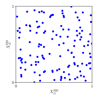
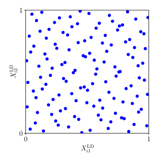
Figure 1: IID points (left) contrasted with LD points (right). The LD points cover the square more evenly.

LD sequences may be deterministic or random, but each point is carefully coordinated with the others so that they fill the domain well. Subsequences of LD sequences are generally not LD. When we say that $\boldsymbol{X}_{0},\boldsymbol{X}_{1},\ldots\overset{\textup{LD}}{\sim}\mathcal{U}[0,1]^{d}$, we mean that for any positive integer $n$, the empirical distribution of $\boldsymbol{X}_{0},\ldots,\boldsymbol{X}_{n-1}$, denoted $F_{\{\boldsymbol{X}_{i}\}_{i=0}^{n-1}}$, approximates the uniform distribution, $F_{\textup{unif}}$, well (relative to $n$). (The empirical distribution of a set assigns equal probability to each point.)

A measure of the difference between the empirical distribution of a set of points and the uniform distribution is called a discrepancy and is denoted $D(\{\boldsymbol{X}_{i}\}_{i=0}^{n-1})$ DicEtal14a ; Hic97a ; Hic99a ; Nie92 . This is the origin of the term “low discrepancy” points or sequences. LD points by definition have a smaller discrepancy than IID points. Fig. 1 contrasts IID uniform points with LD points, $\boldsymbol{X}^{\textup{LD}}_{0},\boldsymbol{X}^{\textup{LD}}_{1}\ldots\overset{\textup{LD}}{\sim}\mathcal{U}[0,1]^{2}$, in this case, linearly scrambled and digitally shifted Sobol’ points.

The error in using the sample mean to approximate the integral can be bounded according to the Koksma-Hlawka inequality and its extensions DicEtal14a ; Hic97a ; Hic99a ; Nie92 as the product of the discrepancy of the sampling sequence and the variation of the integrand, denoted $V(\cdot)$:

$$\lvert\mu-\widehat{\mu}\rvert=\biggl{\lvert}\int_{[0,1]^{d}}f(\boldsymbol{x})\,\mathrm{d}\bigl{(}F_{\textup{unif}}-F_{\{\boldsymbol{X}_{i}\}_{i=0}^{n-1}}\bigr{)}(\boldsymbol{x})\biggr{\rvert}\leq D\bigl{(}\{\boldsymbol{X}_{i}\}_{i=0}^{n-1}\bigr{)}V(f).$$ (5)

The variation is a (semi-) norm of the integrand in a suitable Banach space. The discrepancy corresponds to the norm of the error functional for that Banach space. For typical Banach spaces, the discrepancy of LD points is $\mathcal{O}(n^{-1+\epsilon})$, a higher convergence order than for IID points. For details, readers may refer to the references.

Here, we expect the reader to see in Fig. 1 that the LD points cover the integration domain more evenly than IID points. LD sampling can be thought of as a more even distribution of the sampling sites than IID. LD sampling is similar to stratified sampling. In the examples below, the reader will see the demonstrably smaller cubature errors arising from using LD points.

In the sections that follow, we first overview available QMC software. We next describe an architecture for good QMC software, i.e., what the key components are and how they should interact. We then describe how we have implemented this architecture in QMCPy. Finally, we summarize further directions that we hope QMCPy and other QMC software projects will take. Those interested in following or contributing to the development of QMCPy are urged to visit the GitHub repository at https://github.com/QMCSoftware/QMCSoftware.

We have endeavored to be as accurate as possible at the time of writing this article. We hope that progress in QMC software development will make this article happily obsolete in the coming years.

2 Available Software for QMC

QMC software spans LD sequence generators, cubatures, and applications. Here we review the better-known software, recognizing that some software overlaps multiple categories. Whenever applicable, we state each library’s accessibility in QMCPy, or contrast its functionalities with QMCPy’s — where we lag behind in QMCPy, we strive to catch up in the near future.

Software focusing on generating high-quality LD sequences and their generators includes the following, listed in alphabetical order:

BRODA

Commerical and non-commercial software developed jointly with I.M. Sobol’ in C++, MATLAB, and Excel BRODA20a . BRODA can generate Sobol’ sequences up to 65,536 dimensions. In comparison, QMCPy supports Sobol’ sequences up to 21,201 dimensions.

Burkhardt

Various QMC software for generating van der Corput, Faure, Halton, Hammersley, Niederreiter, or Sobol’ sequences in C, C++, Fortran, MATLAB, or Python Bur20a . In QMCPy, we have implemented digital net, lattice, and Halton generators.

LatNet Builder

The successor to Lattice Builder LEcMun14a , this is a C++ library with Python and Java interfaces (in SSJ below) for generating vectors or matrices for lattices and digital nets LatNet ; LEcEtal22a . QMCPy contains a module for parsing the resultant vectors or matrices from LatNet Builder for compatibility with our LD point generators.

MATLAB

Commercial software for scientific computing MAT9.10 , which contains Sobol’ and Halton sequences in the Statistics and Machine Learning Toolbox. Both generators can be applied jointly with the Parallel Computing Toolbox to accelerate their execution speed. The dimension of the Sobol’ sequences is restricted to 1,111, which is relatively small, yet sufficient for most applications.

MPS

Magic Point Shop contains lattices and Sobol’ sequences in C++, Python, and MATLAB Nuy17a . QMCPy started with MPS for developing LD generators.

Owen

Owen’s randomized Halton sequences with dimensions up to 1,000 Owe20a and scrambled Sobol’ sequences with dimensions up to 21,021 owen1998scrambling ; owen2021r in R. QMCPy supports Owen’s Halton randomization method, and we plan to implement Owen’s nested uniform scrambling for digital nets in the near future.

PyTorch

Open-source Python library for deep learning, with unscrambled or scrambled Sobol’ sequences NEURIPS2019_9015 ; PyTorch . PyTorch enables seamless utilization of Graphics Processing Units (GPUs) or Field Programmable Gate Arrays (FPGAs).

QMC.jl

LD Sequences in Julia Rob20a . Julia bezanson2012julia is an interpreted language similar to Python and R in terms of ease of use, but is designed to run much faster.

qrng

Randomized Sobol’, Halton, and Korobov sequences in R QRNG2020 . The default Halton randomization in QMCPy utilizes the methods from qrng.

SciPy

Scientific computing library in Python with Latin hypercube, Halton, and Sobol’ generators 2020SciPy-NMeth .

TF Quant Finance

Google’s Tensorflow deep-learning library tensorflow2015-whitepaper specialized for financial modeling tfqf21 . It contains lattice and Sobol’ generators alongside with algorithms sped up with GPUs, FGPAs, or Tensor Processing Units (TPUs).

Software focusing on QMC cubatures and applications includes the following:

GAIL

The Guaranteed Automatic Integration Library contains automatic (Q)MC stopping criteria in MATLAB ChoEtal21a ; HCJJ14 . These are iterative procedures for one- or high-dimensional integration that take a user’s input error tolerance(s) and determine the number of (Q)MC sampling points necessary to achieve user-desired accuracy (almost surely). Most of GAIL’s (Q)MC functions, some with enhancements, are implemented in Python in QMCPy.

ML(Q)MC

Multi-Level (Q)MC routines in C, C++, MATLAB, Python, and R GilesSoft . We have ported ML(Q)MC functions to QMCPy.

MultilevelEstimators.jl

ML(Q)MC methods in Julia Rob21 . The author, Pieterjan Robbe, has contributed cubature algorithms and use cases to QMCPy.

OpenTURNS

Open source initiative for the Treatment of Uncertainties, Risks’N Statistics OpenTURNS written in C++ and Python, leveraging R statistical packages, as well as LAPACK and BLAS for numerical linear algebra.

QMC4PDE

QMC for elliptic PDEs with random diffusion coefficients in Python KuoNuy16a .

SSJ

Stochastic Simulation with the hups package in Java SSJ .

UQLab

Framework for Uncertainty Quantification in MATLAB UQLab2014 . The core of UQLab is closed source, but a large portion of the library is open source. Recently, UQ[py]Lab, the beta release of UQLab with Python bindings, is available as Software as a Service (SaaS) via UQCloud lataniotis2021uncertainty .

The sections that follow describe QMCPy QMCPy2020a , which is our attempt to establish a framework for QMC software and to combine the best of the above software under a common user interface written in Python 3. The choice of language was determined by the desire to make QMC software accessible to a broad audience, especially the technology industry.

3 Components of QMC Software

QMC cubature can be summarized as follows. We want to approximate the expectation, $\mu$, well by the sample mean, $\widehat{\mu}$, where (1), (2), and (3) combine to give

$$\mu:=\int_{\mathcal{T}}g(\boldsymbol{t})\,\lambda(\boldsymbol{t})\,\mathrm{d}\boldsymbol{t}=\mathbb{E}[f(\boldsymbol{X})]=\int_{[0,1]^{d}}f(\boldsymbol{x})\,\mathrm{d}\boldsymbol{x}\approx\frac{1}{n}\sum_{i=0}^{n-1}f(\boldsymbol{X}_{i})=:\widehat{\mu},\\ \boldsymbol{X}\sim\mathcal{U}[0,1]^{d},\ \boldsymbol{X}_{0},\boldsymbol{X}_{1},\ldots\overset{\textup{M}}{\sim}\mathcal{U}[0,1]^{d}.$$ (6)

Moreover, we want to satisfy the error requirement in (4). This requires four components, which we implement as QMCPy classes.

Discrete Distribution

produces the sequence $\boldsymbol{X}_{0},\boldsymbol{X}_{1},\dots$ that mimics $\mathcal{U}[0,1]^{d}$;

True Measure

$\boldsymbol{t}\mapsto\lambda(\boldsymbol{t})\mathrm{d}\boldsymbol{t}$ defines the original measure, e.g., Gaussian or Lebesgue;

Integrand

$g$ defines the original integrand, and $f$ defines the transformed version to fit the DiscreteDistribution; and

Stopping Criterion

determines how large $n$ should be to ensure that $\lvert\mu-\widehat{\mu}\rvert\leq\varepsilon$ as in (4).

The software libraries referenced in Section 2 provide one or more of these components. QMCPy combines multiple examples of all these components under an object-oriented framework. Each example is implemented as a concrete class that realizes the properties and methods required by the abstract class for that component. The following sections detail descriptions and specific examples for each component.

Thorough documentation of all QMCPy classes is available in QMCPyDocs . Demonstrations of how QMCPy works are given in Google Colab notebooks QMCPyTutColab2020 ; QMCPyTutColab2020_paper . The project may be installed from PyPI into a Python 3 environment via the command pip install qmcpy. In the code snippets that follow, we assume QMCPy has been imported alongside NumPy numpy via the following commands in a Python Console:

⬇

cyan>>> blueimport qmcpy blueas qp

cyan>>> blueimport numpy blueas np

4 Discrete Distributions

LD sequences typically mimic $\mathcal{U}[0,1]^{d}$. Good sequences mimicking other distributions are obtained by transformations as described in the next section. We denote by DiscreteDistribution the abstract class containing LD sequence generators. In most cases that have been implemented, the points $\boldsymbol{X}_{0},\ldots,\boldsymbol{X}_{n-1}$ have an empirical (discrete) distribution that closely approximates the uniform distribution, say, in the sense of discrepancy. We also envision future possible DiscreteDistribution objects that assign unequal weights to the sampling points. In any case, the term “discrete” refers to the fact that these are sequences of points (and weights), not continuous distributions.

QMCPy implements extensible LD sequences, i.e., those that allow practitioners to obtain and use $\boldsymbol{X}_{n},\boldsymbol{X}_{n+1},\ldots$ without discarding $\boldsymbol{X}_{0},\ldots,\boldsymbol{X}_{n-1}$. Halton sequences do not have preferred sample sizes $n$, but extensible integration lattices and digital sequences in base $b$ prefer $n$ to be a power of $b$. For integration lattices and digital sequences, we have focused on base $b=2$ since this is a popular choice and for convenience in generating extensible sequences.

Integration lattices and digital sequences in base $2$ have an elegant group structure, which we summarize in Table 1. The addition operator is $\oplus$, and its inverse is $\ominus$. The unshifted sequence is $\boldsymbol{Z}_{0},\boldsymbol{Z}_{1},\ldots$ and the randomly shifted sequence is $\boldsymbol{X}_{0},\boldsymbol{X}_{1},\ldots$

Table 1: Properties of lattices and digital net sequences. Note that they share group properties but also have distinctives.

$$\begin{array}[]{c@{\qquad}c}\hline\cr\lx@intercol\hfil\text{Define \ldots}\hfil\lx@intercol\\ \lx@intercol\hfil\boldsymbol{Z}_{1},\boldsymbol{Z}_{2},\boldsymbol{Z}_{4},\ldots\in[0,1)^{d}\text{ chosen well}\hfil\lx@intercol\\ \lx@intercol\hfil\boldsymbol{Z}_{i}:=i_{0}\boldsymbol{Z}_{1}\oplus i_{1}\boldsymbol{Z}_{2}\oplus i_{2}\boldsymbol{Z}_{4}\oplus i_{3}\boldsymbol{Z}_{8}\oplus\cdots\quad\text{for }i=i_{0}+i_{1}2+i_{2}4+i_{3}8+\cdots,\;i_{\ell}\in\{0,1\}\hfil\lx@intercol\\ \lx@intercol\hfil\boldsymbol{X}_{i}:=\boldsymbol{Z}_{i}\oplus\boldsymbol{\Delta},\qquad\text{where }\boldsymbol{\Delta}\overset{\textup{IID}}{\sim}[0,1)^{d}\hfil\lx@intercol\\ \hline\cr\text{Rank-1 Integration Lattices}&\text{Digital Nets}\\ \boldsymbol{t}\oplus\boldsymbol{x}:=(\boldsymbol{t}+\boldsymbol{x})\bmod\boldsymbol{1}&\boldsymbol{t}\oplus\boldsymbol{x}:=\text{binary digitwise addition},\oplus_{\textup{dig}}\\ \text{require }\boldsymbol{Z}_{2^{m}}\oplus\boldsymbol{Z}_{2^{m}}=\boldsymbol{Z}_{\lfloor 2^{m-1}\rfloor}\quad\forall m\in\mathbb{N}_{0}\\[2.15277pt] \hline\cr\lx@intercol\hfil\text{Then it follows that \ldots}\hfil\lx@intercol\\ \lx@intercol\hfil\left.\begin{array}[]{r}\mathcal{P}_{m}:=\{\boldsymbol{Z}_{0},\ldots,\boldsymbol{Z}_{2^{m}-1}\},\quad\boldsymbol{Z}_{i}\oplus\boldsymbol{Z}_{j}\in\mathcal{P}_{m}\\ \mathcal{P}_{\boldsymbol{\Delta},m}:=\{\boldsymbol{X}_{0},\ldots,\boldsymbol{X}_{2^{m}-1}\},\quad\boldsymbol{X}_{i}\oplus\boldsymbol{X}_{j}\ominus\boldsymbol{X}_{k}\in\mathcal{P}_{\boldsymbol{\Delta},m}\end{array}\right\}\quad\begin{array}[]{l}\forall i,j,k\in\{0,\ldots,2^{m}-1\}\\ \forall m\in\mathbb{N}_{0}\end{array}\hfil\lx@intercol\\ \hline\cr\end{array}$$

We illustrate lattice and Sobol’ sequences using QMCPy. First, we create an instance of a $d=2$ dimensional Lattice object of the DiscreteDistribution abstract class. Then we generate the first eight (non-randomized) points in this lattice.

⬇

cyan>>> lattice = qp.Lattice(dimension=2, randomize=False)

cyan>>> lattice.gen_samples(n=8)

darkgreen"ParameterWarning:

Non-randomized lattice sequence includes the origin"

array([[0. , 0. ],

[0.5 , 0.5 ],

[0.25 , 0.75 ],

[0.75 , 0.25 ],

[0.125, 0.375],

[0.625, 0.875],

[0.375, 0.125],

[0.875, 0.625]])

The first three generators for this lattice are $\boldsymbol{Z}_{1}=(0.5,0.5)$, $\boldsymbol{Z}_{2}=(0.25,0.75)$, and $\boldsymbol{Z}_{4}=(0.125,0.375)$. One can check that $(\boldsymbol{Z}_{2}+\boldsymbol{Z}_{4})\bmod\boldsymbol{1}=(0.375,0.125)=\boldsymbol{Z}_{6}$, as Table 1 specifies.

The random shift has been turned off above to illuminate the group structure. We normally include the randomization to ensure that there are no points on the boundary of $[0,1]^{d}$. Then, when points are transformed to mimic distributions such as the Gaussian, no LD points will be transformed to infinity. Turning off the randomization generates a warning when the gen_samples method is called.

Now, we generate Sobol’ points using a similar process as we did for lattice points. Sobol’ sequences are one of the most popular example of digital sequences.

⬇

cyan>>> sobol = qp.Sobol(2, randomize=False)

cyan>>> sobol.gen_samples(8, warn=False)

array([[0. , 0. ],

[0.5 , 0.5 ],

[0.25 , 0.75 ],

[0.75 , 0.25 ],

[0.125, 0.625],

[0.625, 0.125],

[0.375, 0.375],

[0.875, 0.875]])

Here, $\boldsymbol{Z}_{4}$ differs from that for lattices, but more importantly, addition for digital sequences differs from that for lattices. Using digitwise addition for digital sequences, we can confirm that according to Table 1,

$$\boldsymbol{Z}_{2}\oplus_{\textup{dig}}\boldsymbol{Z}_{4}=(0.25,0.75)\oplus_{\textup{dig}}(0.125,0.625)$$

$$=({}_{2}0.010,{}_{2}0.110)\oplus_{\textup{dig}}({}_{2}0.001,{}_{2}0.101) =({}_{2}0.011,{}_{2}0.011)$$

$$=(0.375,0.375)=\boldsymbol{Z}_{6}.$$

By contrast, if we construct a digital sequence using the generators for the lattice above with $\boldsymbol{Z}_{2}=(0.25,0.75)$, and $\boldsymbol{Z}_{4}=(0.125,0.375)$, we would obtain

$$\boldsymbol{Z}_{6}=\boldsymbol{Z}_{2}\oplus_{\textup{dig}}\boldsymbol{Z}_{4}=({}_{2}0.010,{}_{2}0.110)\oplus_{\textup{dig}}({}_{2}0.001,{}_{2}0.011)\\ =({}_{2}0.011,{}_{2}0.101)=(0.375,0.625),$$

which differs from the $\boldsymbol{Z}_{6}=(0.375,0.125)$ constructed for lattices. To emphasize, lattices and digital sequences are different, even if they share the same generators, $\boldsymbol{Z}_{1},\boldsymbol{Z}_{2},\boldsymbol{Z}_{4},\ldots$.

The examples of qp.Lattice and qp.Sobol illustrate how QMCPy LD generators share a common user interface. The dimension is specified when the instance is constructed, and the number of points is specified when the gen_samples method is called. Following Python practice, parameters can be input without specifying their names if input in the prescribed order. QMCPy also includes Halton sequences and IID sequences, again deferring details to the QMCPy documentation QMCPyDocs .

A crucial difference between IID generators and LD generators is reflected in the behavior of generating $n$ points. For an IID generator, asking for $n$ points repeatedly gives different points each time because they are meant to be random and independent.

⬇

cyan>>> iid = qp.IIDStdUniform(2); iid.gen_samples(1)

array([[0.40538109, 0.12255759]])

cyan>>> iid.gen_samples(1)

array([[0.50913741, 0.11312201]])

Your output may look different depending on the seed used to generate these random numbers.

On the other hand, for an LD generator, asking for $n$ points repeatedly gives the same points each time because they are meant to be the first $n$ points of a specific LD sequence.

⬇

cyan>>> lattice = qp.Lattice(2); lattice.gen_samples(1)

array([[0.2827584 , 0.36731649]])

cyan>>> lattice.gen_samples(1)

array([[0.2827584 , 0.36731649]])

Here we allow the randomization so that the first point in the sequence is not the origin. To obtain the next $n$ points, one may specify the start and ending indices of the sequence.

⬇

cyan>>> lattice.gen_samples(2)

array([[0.2827584 , 0.36731649],

[0.7827584 , 0.86731649]])

cyan>>> lattice.gen_samples(n_min=1, n_max=2)

array([[0.7827584 , 0.86731649]])

Fig. 2 shows how increasing the number of lattice and Sobol’ LD points through powers of two fills in the gaps in an even way.

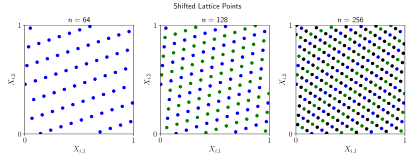
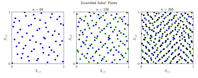
Figure 2: Randomized lattice and Sobol’ points mimicking a $\mathcal{U}[0,1]^{2}$ measure for $n=64,128,$ and 256. Note how increasing the number of points evenly fills in the gaps between the points.

5 True Measures

The LD sequences implemented as DiscreteDistribution objects mimic the $\mathcal{U}[0,1]^{d}$ distribution. However, we may need sequences to mimic other distributions. This is implemented via variable transformations, $\boldsymbol{\Psi}$. In general, if $\boldsymbol{X}\overset{\textup{M}}{\sim}\mathcal{U}[0,1]^{d}$, then

$$\boldsymbol{T}=\boldsymbol{\Psi}(\boldsymbol{X}):=\boldsymbol{a}+(\boldsymbol{b}-\boldsymbol{a})\odot\boldsymbol{X}\overset{\textup{M}}{\sim}\mathcal{U}[\boldsymbol{a},\boldsymbol{b}],$$ (7a)

$$\boldsymbol{T}=\boldsymbol{\Psi}(\boldsymbol{X}):=\boldsymbol{a}+\mathsf{A}\boldsymbol{\Phi}^{-1}(\boldsymbol{X})\overset{\textup{M}}{\sim}\mathcal{N}(\boldsymbol{a},\Sigma),$$ (7b)

$$\text{where }\boldsymbol{\Phi}^{-1}(\boldsymbol{X}):=\begin{pmatrix}\Phi^{-1}(X_{1})\\ \vdots\\ \Phi^{-1}(X_{d})\end{pmatrix},\qquad\Sigma=\mathsf{A}\mathsf{A}^{T},$$

and $\odot$ denotes term-by-term (Hadamard) multiplication. Here, $\boldsymbol{a}$ and $\boldsymbol{b}$ are assumed to be finite, and $\Phi$ is the standard Gaussian distribution function. Again we use $\overset{\textup{M}}{\sim}$ to denote mimicry, not necessarily in a probabilistic sense.

Fig. 3 displays LD sequences transformed as described above to mimic a uniform and a Gaussian distribution. The code to generate these points takes the following form for uniform points based on a Halton sequence:

⬇

cyan>>> u = qp.Uniform(

cyan... sampler = qp.Halton(2),

cyan... lower_bound = [-2, 0],

cyan... upper_bound = [2, 4])

cyan>>> u.gen_samples(4)

array([[ 1.80379772, 3.51293599],

[-0.19620228, 0.84626932],

[ 0.80379772, 2.17960265],

[-1.19620228, 3.95738043]])

whereas for Gaussian points based on a lattice sequence, we have:

⬇

cyan>>> g = qp.Gaussian(qp.Lattice(2),

cyan... mean = [3, 2],

cyan... covariance = [[9, 5],

cyan... [5, 4]])

cyan>>> g.gen_samples(4)

array([[-0.00920667, 0.29392389],

[ 5.02422481, 1.45408341],

[ 6.53688109, 5.14785917],

[ 2.58403124, 1.16941969]])

Here the covariance decomposition $\Sigma=\mathsf{A}\mathsf{A}^{T}$ is done using principal component analysis. The Cholesky decomposition is also available.

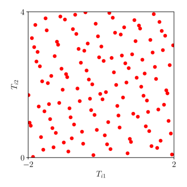
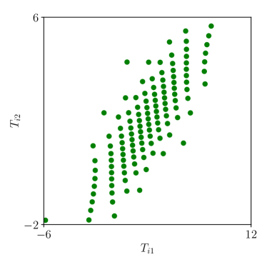
Figure 3: Halton samples transformed to mimic a uniform $\mathcal{U}\left(\begin{bmatrix}-2\\ 0\end{bmatrix},\begin{bmatrix}2\\ 4\end{bmatrix}\right)$ distribution (left) and lattice samples transformed to mimic a Gaussian $\mathcal{N}\left(\begin{bmatrix}3\\ 2\end{bmatrix},\begin{bmatrix}9&5\\ 5&4\end{bmatrix}\right)$ distribution (right).

The Brownian motion distribution arises often in financial risk applications. Here the $d$ components of the variable $\boldsymbol{T}$ correspond to the discretized Brownian motion at times $\tau/d,2\tau/d,\ldots,\tau$, where $\tau$ is the time horizon. The distribution is a special case of the Gaussian with covariance

$$\Sigma=(\tau/d)\bigl{(}\min(j,k)\bigr{)}_{j,k=1}^{d}$$ (8)

and mean $\boldsymbol{a}$, which is proportional to the times $(\tau/d)(1,2,\ldots,d)^{T}$. The code for generating a Brownian motion is

⬇

cyan>>> bm = qp.BrownianMotion(qp.Sobol(4), drift=2)

cyan>>> bm.gen_samples(2)

array([[-0.28902829, 0.48582198, 1.81113976, 2.2376372 ],

[ 1.41552651, 1.93926124, 1.27619672, 1.47496128]])

Fig. 4 displays a Brownian motion based on Sobol’ sequence with and without a drift.

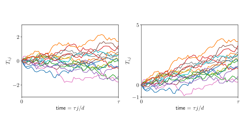
Figure 4: Sobol’ samples transformed to mimic a 52-dimensional Brownian Motion without drift (left) and with drift coefficient 2 (right).

6 Integrands

Let’s return to the integration problem in (1), which we must rewrite as (2). We choose a transformation of variables defined as $\boldsymbol{t}=\boldsymbol{\Psi}(\boldsymbol{x})$ where $\boldsymbol{\Psi}:[0,1]^{d}\to\mathcal{T}$. This leads to

$$\mu =\int_{\mathcal{T}}g(\boldsymbol{t})\,\lambda(\boldsymbol{t})\,\mathrm{d}\boldsymbol{t}=\int_{[0,1]^{d}}g\bigl{(}\boldsymbol{\Psi}(\boldsymbol{x})\bigr{)}\,\lambda\bigl{(}\boldsymbol{\Psi}(\boldsymbol{x})\bigr{)}\,\lvert\boldsymbol{\Psi}^{\prime}(\boldsymbol{x})\rvert\,\mathrm{d}\boldsymbol{x}=\int_{[0,1]^{d}}f(\boldsymbol{x})\,\mathrm{d}\boldsymbol{x},$$

$$\qquad\qquad\text{where }f(\boldsymbol{x})=g\bigl{(}\boldsymbol{\Psi}(\boldsymbol{x})\bigr{)}\,\lambda\bigl{(}\boldsymbol{\Psi}(\boldsymbol{x})\bigr{)}\,\lvert\boldsymbol{\Psi}^{\prime}(\boldsymbol{x})\rvert,$$ (9)

and $\lvert\boldsymbol{\Psi}^{\prime}(\boldsymbol{x})\rvert:=\lvert\partial\boldsymbol{\Psi}/\partial\boldsymbol{x}\rvert$ represents the Jacobian of the variable transformation. The abstract class Integrand provides $f$ based on the user’s input of $g$ and the TrueMeasure instance, which defines $\lambda$ and the transformation $\boldsymbol{\Psi}$. Different choices of $\boldsymbol{\Psi}$ lead to different $f$, which may give different rates of convergence of the cubature, $\widehat{\mu}$ to $\mu$.

We illustrate the Integrand class via an example of Keister Kei96 :

$$\mu=\int_{\mathbb{R}^{d}}\cos(\lVert\boldsymbol{t}\rVert)\exp(-\boldsymbol{t}^{T}\boldsymbol{t})\,\mathrm{d}\boldsymbol{t}\\ =\int_{\mathbb{R}^{d}}\underbrace{\pi^{d/2}\cos(\lVert\boldsymbol{t}\rVert)}_{g(\boldsymbol{t})}\,\underbrace{\pi^{-d/2}\exp(-\boldsymbol{t}^{T}\boldsymbol{t})}_{\lambda(\boldsymbol{t})}\,\mathrm{d}\boldsymbol{t}.$$ (10)

Since $\lambda$ is the density for $\mathcal{N}(\boldsymbol{0},\mathsf{I}/2)$, it is natural to choose $\boldsymbol{\Psi}$ according to (7b) with $\mathsf{A}=\sqrt{1/2}\,\mathsf{I}$, in which case $\lambda(\boldsymbol{\Psi}(\boldsymbol{x}))\lvert\boldsymbol{\Psi}^{\prime}(\boldsymbol{x})\rvert=1$, and so

$$\mu=\int_{[0,1]^{d}}\underbrace{\pi^{d/2}\cos(\lVert\boldsymbol{\Psi}(\boldsymbol{x})\rVert)}_{f(\boldsymbol{x})}\,\mathrm{d}\boldsymbol{x},\qquad\boldsymbol{\Psi}(\boldsymbol{x}):=\sqrt{1/2}\,\boldsymbol{\Phi}^{-1}(\boldsymbol{x}).$$

The code below sets up an Integrand instance using QMCPy’s CustomFun wrapper to tie a user-defined function $g$ into the QMCPy framework. Then we evaluate the sample mean of $n=1000$ $f$ values obtained by sampling at transformed Halton points. Notice how a two-dimensional Halton generator is used to construct a Gaussian true measure, which is applied alongside the my_Keister function to instantiate a customized, QMCPy-compatible integrand for this problem.

⬇

cyan>>> bluedef my_Keister(t):

cyan... d = t.shape[1] darkgreen# t is an (n x d) array

cyan... norm = np.sqrt((t**2).sum(1))

cyan... out = np.pi**(d/2)*np.cos(norm)

cyan... bluereturn out darkgreen# size n vector

cyan...

cyan>>> gauss = qp.Gaussian(qp.Halton(2), covariance=1/2)

cyan>>> keister = qp.CustomFun(true_measure=gauss, g=my_Keister)

cyan>>> x = keister.discrete_distrib.gen_samples(1000)

cyan>>> y = keister.f(x)

cyan>>> y.mean()

1.809055768468628

We have no indication yet of how accurate our approximation is. That topic is treated in the next section. Fig. 5 visualizes sampling on the original integrand, $g$, and sampling on the transformed integrand, $f$.

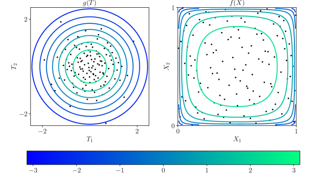
Figure 5: Right: Sampling the transformed Keister integrand $f$ at Halton points $\boldsymbol{X}_{i}\overset{\textup{LD}}{\sim}\mathcal{U}[0,1]^{2}$. Left: Sampling the original Keister integrand $g$ at $\boldsymbol{T}_{i}=\boldsymbol{\Psi}(\boldsymbol{X}_{i})\overset{\textup{M}}{\sim}\mathcal{N}(\boldsymbol{0},\mathsf{I}/2)$ where $\boldsymbol{\Psi}$ is defined in (7b).

Another way to approximate the Keister integral in (10) is to write it as an integral with respect to the Lebesgue measure:

$$\mu =\int_{\mathbb{R}^{d}}\underbrace{\cos(\lVert\boldsymbol{t}\rVert)\exp(-\boldsymbol{t}^{T}\boldsymbol{t})}_{g(\boldsymbol{t})}\,\underbrace{1}_{\lambda(\boldsymbol{t})}\,\mathrm{d}\boldsymbol{t}$$

$$=\int_{[0,1]^{d}}\underbrace{\cos(\lVert\boldsymbol{\Psi}(\boldsymbol{x})\rVert)\exp(-\boldsymbol{\Psi}^{T}\!\!(\boldsymbol{x})\boldsymbol{\Psi}(\boldsymbol{x}))\lvert\boldsymbol{\Psi}^{\prime}(\boldsymbol{x})\rvert}_{f(\boldsymbol{x})}\,\mathrm{d}\boldsymbol{x},$$

where $\boldsymbol{\Psi}$ is any transformation from $[0,1]^{d}$ to $\mathbb{R}^{d}$. Now $\lambda$ is not a PDF. QMCPy can perform the cubature this way as well.

⬇

cyan>>> bluedef my_L_Keister(t):

cyan... norm_sq = (t**2).sum(1)

cyan... out = np.cos(np.sqrt(norm_sq))*np.exp(-norm_sq)

cyan... bluereturn out

cyan...

cyan>>> lebesgue_gauss = qp.Lebesgue(qp.Gaussian(qp.Halton(2)))

cyan>>> keister = qp.CustomFun(lebesgue_gauss, my_L_Keister)

cyan>>> x = keister.discrete_distrib.gen_samples(1000)

cyan>>> y = keister.f(x)

cyan>>> y.mean()

1.8056340581961572

The $\boldsymbol{\Psi}$ chosen when transforming uniform sequences on the unit cube to fill $\mathbb{R}^{d}$ is given by (7b) with $\mathsf{A}=\mathsf{I}$.

In the examples above, one must input the correct $g$ into CustomFun along with the correct TrueMeasure $\lambda$ to define the integration problem. The Keister integrand included in the QMCPy library takes a more flexible approach to defining the integration problem $\mu$ in (10). Selecting a different sampler $\boldsymbol{\Psi}$ performs importance sampling, which leaves $\mu$ unchanged.

⬇

cyan>>> darkgreen# default transform

cyan>>> keister = qp.Keister(qp.Halton(2))

cyan>>> x = keister.discrete_distrib.gen_samples(1e4)

cyan>>> keister.f(x).mean()

1.8082377673556123

cyan>>> darkgreen# custom transform for importance sampling

>>> keister = qp.Keister(sampler=qp.Gaussian(qp.Halton(2)))

cyan>>> x = keister.discrete_distrib.gen_samples(1e4)

cyan>>> keister.f(x).mean()

1.8080555069060817

In the first case above, the $\lambda$ in (9) corresponds to the Gaussian density with mean zero and variance $1/2$ by default, and the corresponding variable transformation, $\boldsymbol{\Psi}$, is chosen to make $\lambda\bigl{(}\boldsymbol{\Psi}(\boldsymbol{x})\bigr{)}\lvert\boldsymbol{\Psi}^{\prime}(\boldsymbol{x})\rvert=1$ and $f(\boldsymbol{x})=g\left(\boldsymbol{\Psi}(\boldsymbol{x})\right)$. In the second case, we choose an importance sampling density $\lambda_{\textup{IS}}$, corresponding to standard Gaussian, and the variable transformation $\boldsymbol{\Psi}_{\textup{IS}}$ makes $\lambda_{\textup{IS}}\bigl{(}\boldsymbol{\Psi}_{\textup{IS}}(\boldsymbol{x})\bigr{)}\lvert\boldsymbol{\Psi}^{\prime}_{\textup{IS}}(\boldsymbol{x})\rvert=1$. Then

$$\mu =\int_{\mathcal{T}}g(\boldsymbol{t})\,\lambda(\boldsymbol{t})\,\mathrm{d}\boldsymbol{t}=\int_{\mathcal{T}}g(\boldsymbol{t})\,\frac{\lambda(\boldsymbol{t})}{\lambda_{\textup{IS}}(\boldsymbol{t})}\,\lambda_{\textup{IS}}(\boldsymbol{t})\mathrm{d}\boldsymbol{t}$$

$$=\int_{[0,1]^{d}}g\bigl{(}\boldsymbol{\Psi}_{\textup{IS}}(\boldsymbol{x})\bigr{)}\,\frac{\lambda\bigl{(}\boldsymbol{\Psi}_{\textup{IS}}(\boldsymbol{x})\bigr{)}}{\lambda_{\textup{IS}}\bigl{(}\boldsymbol{\Psi}_{\textup{IS}}(\boldsymbol{x})\bigr{)}}\lambda_{\textup{IS}}\bigl{(}\boldsymbol{\Psi}_{\textup{IS}}(\boldsymbol{x})\bigr{)}\,\lvert\boldsymbol{\Psi}^{\prime}_{\textup{IS}}(\boldsymbol{x})\rvert\,\mathrm{d}\boldsymbol{x}$$

$$=\int_{[0,1]^{d}}f_{\textup{IS}}(\boldsymbol{x})\,\mathrm{d}\boldsymbol{x}$$

$$\qquad\qquad\text{where }f_{\textup{IS}}(\boldsymbol{x})=g\bigl{(}\boldsymbol{\Psi}_{\textup{IS}}(\boldsymbol{x})\bigr{)}\,\frac{\lambda\bigl{(}\boldsymbol{\Psi}_{\textup{IS}}(\boldsymbol{x})\bigr{)}}{\lambda_{\textup{IS}}\bigl{(}\boldsymbol{\Psi}_{\textup{IS}}(\boldsymbol{x})\bigr{)}}.$$ (11)

Because LD samples mimic $\mathcal{U}[0,1]^{d}$, choosing a different sampler is equivalent to choosing a different variable transform.

7 Stopping Criteria

The StoppingCriterion object determines the number of samples $n$ that are required for the sample mean approximation $\widehat{\mu}$ to be within error tolerance $\varepsilon$ of the true mean $\mu$. Several QMC stopping criteria have been implemented in QMCPy, including replications, stopping criteria that track the decay of the Fourier complex exponential or Walsh coefficients of the integrand HicJim16a ; HicEtal17a ; JimHic16a , and stopping criteria based on Bayesian credible intervals RatHic19a ; JagHic22a .

The CubQMCSobolG stopping criterion used in the example below assumes the Walsh-Fourier coefficients of the integrand are absolutely convergent. The algorithm iteratively doubles the number of samples used in the integration and estimates the error using the decay of the Walsh coefficients HicJim16a . When the estimated error is below the user-specified tolerance, it finishes the computation and returns the estimated integral.

Let us return to the Keister example from the previous section. After setting up a default Keister instance via a Sobol’ DiscreteDistribution, we choose a StoppingCriterion object that matches the DiscreteDistribution and input our desired tolerance. Calling the integrate method returns the approximate integral plus some useful information about the computation.

⬇

cyan>>> keister = qp.Keister(qp.Sobol(2))

cyan>>> stopping = qp.CubQMCSobolG(keister, abs_tol=1e-3)

cyan>>> solution_qmc,data_qmc = stopping.integrate()

cyan>>> data_qmc darkgreen# equivalent to print(data_qmc)

LDTransformData (AccumulateData Object)

solution 1.808

error_bound 6.06e-04

n_total 2^(13)

time_integrate 0.008

CubQMCSobolG (StoppingCriterion Object)

abs_tol 0.001

rel_tol 0

n_init 2^(10)

n_max 2^(35)

Keister (Integrand Object)

Gaussian (TrueMeasure Object)

mean 0

covariance 2^(-1)

decomp_type PCA

Sobol (DiscreteDistribution Object)

d 2^(1)

dvec [0 1]

randomize LMS_DS

graycode 0

entropy 326942311248945520670220938885737472885

spawn_key ()

The second output of the stopping criterion provides helpful diagnostic information. This computation requires $n=2^{13}$ Sobol’ points and $0.008$ seconds to complete. The error bound is $0.000606$, which falls below the absolute tolerance.

QMC, which uses LD sequences, is touted as providing substantially greater computational efficiency compared to IID MC. Fig. 6 compares the time and sample sizes needed to compute the $5$-dimensional Keister integral (10) using IID sequences and LD lattice sequences. Consistent with what is stated in Section 1, the error of IID MC is $\mathcal{O}(n^{-1/2})$, which means that the time and sample size to obtain an absolute error tolerance of $\varepsilon$ is $\mathcal{O}(\varepsilon^{-2})$. By contrast, the error of QMC using LD sequences is $\mathcal{O}(n^{-1+\epsilon})$, which implies $\mathcal{O}(\varepsilon^{-1-\epsilon})$ times and sample sizes. We see that QMC methods often require orders of magnitude fewer samples than MC methods to achieve the same error tolerance.

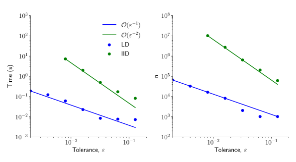
Figure 6: Comparison of run times and sample sizes for computing the $5$-dimensional Keister integral (10) using IID and LD lattice sequences for a variety of absolute error tolerances. The respective stopping criteria are qp.CubMCG HicEtal14a and qp.CubQMCLatticeG JimHic16a . The LD sequences provide the desired answer much more efficiently.

For another illustration of QMC cubature, we turn to pricing an Asian arithmetic mean call option. The (continuous-time) Asian option is defined in terms of the average of the stock price, which is written in terms of an integral. The payoff of this option is the positive difference between the strike price, $K$, averaged over the time horizon:

$$\text{payoff}(\boldsymbol{S})=\max\left(\frac{1}{2d}\sum_{j=1}^{d}(S_{j-1}+S_{j})-K,\;0\right),\quad\boldsymbol{S}=(S_{0},\ldots,S_{d}).$$

Here $S_{j}$ denotes the asset price at time $\tau j/d$, and a trapezoidal rule is used for discrete approximation of the integral in time that defines the average. The trapezoidal rule is a more accurate approximation to the integral than a rectangle rule. A basic model for asset prices is a geometric Brownian motion,

$$S_{j}(\boldsymbol{T})=S_{0}\exp((r-\sigma^{2}/2)\tau j/d+\sigma T_{j}),\;j=1,\ldots,d,\;\boldsymbol{T}=(T_{1},\ldots,T_{d})\sim\mathcal{N}(\boldsymbol{0},\Sigma),$$

where $\Sigma$ is defined in (8), $r$ is the interest rate, $\sigma$ is the volatility, and $S_{0}$ is the initial asset price. The fair price of the option is then the expected value of the discounted payoff, namely,

$$\text{price}=\mu=\mathbb{E}[g(\boldsymbol{T})],\quad\text{where }g(\boldsymbol{t})=\text{payoff}\bigl{(}\boldsymbol{S}(\boldsymbol{t})\bigr{)}\exp(-r\tau).$$

The following code utilizes QMCPy’s Asian option Integrand object to approximate the value of an Asian call option for a particular choice of the parameters.

⬇

cyan>>> payoff = qp.AsianOption(

cyan... qp.Sobol(52), darkgreen# weekly monitoring

cyan... start_price = 100,

cyan... strike_price = 120,

cyan... volatility = 0.5,

cyan... interest_rate = 0,

cyan... t_final = 1,

cyan... call_put = darkgreen"call")

cyan>>> qmc_stop_crit = qp.CubQMCSobolG(payoff, abs_tol=0.001)

cyan>>> price,data = qmc_stop_crit.integrate()

cyan>>> blueprint(darkgreen"Option price = $%.3f using %.3f seconds, %.2e samples"

cyan... %(price, data.time_integrate, data.n_total))

Option price = $5.194 using 0.587 seconds, 1.31e+05 samples

Because this Integrand object has the built-in Brownian motion TrueMeasure, one only need provide the LD sampler.

Out of the money option price calculations can be sped up by adding an upward drift to the Brownian motion. The upward drift produces more in the money paths and also reduces the variation or variance of the final integrand, $f$. This is a form of importance sampling. Using a Brownian motion without drift we get

⬇

cyan>>> payoff = qp.AsianOption(qp.Sobol(52),

cyan... start_price=100, strike_price=200)

cyan>>> qmc_stopper = qp.CubQMCSobolG(payoff, abs_tol=0.001)

cyan>>> price,data = qmc_stopper.integrate()

cyan>>> blueprint(darkgreen"Option price = $%.4f using %.3f seconds, n = %.2e"

cyan... %(price, data.time_integrate, data.n_total))

Option price = $0.1757 using 0.583 seconds, n = 1.31e+05

Adding the upward drift gives us the answer faster:

⬇

cyan>>> payoff = qp.AsianOption(

cyan... sampler = qp.BrownianMotion(qp.Sobol(52), drift=1),

cyan... start_price=100, strike_price=200)

cyan>>> qmc_stopper = qp.CubQMCSobolG(payoff, abs_tol=0.001)

cyan>>> price,data_drift = qmc_stopper.integrate()

cyan>>> blueprint(darkgreen"Option price = $%.4f using %.3f seconds, n = %.2e"

cyan... %(price, data_drift.time_integrate, data_drift.n_total))

Option price = $0.1754 using 0.085 seconds, n = 1.64e+04

cyan>>> blueprint(darkgreen"Using drift required %.0f%% the time, %.0f%% the n"

cyan... %(100*data_drift.time_integrate / data.time_integrate,

cyan... 100*data_drift.n_total / data.n_total))

Using drift required 15% the time, 12% the n

The choice of a good drift is an art.

The improvement in time is less than that in $n$ because the integrand is more expensive to compute when the drift is employed. Referring to (11), in the case of no drift, the $\lambda$ corresponds to the density for the discrete Brownian motion, and the variable transformation $\boldsymbol{\Psi}$ is chosen so that $f(\boldsymbol{x})=g\left(\boldsymbol{\Psi}(\boldsymbol{x})\right)$. However, in the case of a drift, the integrand becomes $f_{\textup{IS}}(\boldsymbol{x})=g\bigl{(}\boldsymbol{\Psi}_{\textup{IS}}(\boldsymbol{x})\bigr{)}\lambda\bigl{(}\boldsymbol{\Psi}_{\textup{IS}}(\boldsymbol{x})\bigr{)}/\lambda_{\textup{IS}}\bigl{(}\boldsymbol{\Psi}_{\textup{IS}}(\boldsymbol{x})\bigr{)}$, which requires more computation time per integrand value.

8 Under the Hood

In this section, we look at the inner workings of QMCPy and point out features we hope will benefit the community of QMC researchers and practitioners. We also highlight important nuances of QMC methods and how QMCPy addresses these challenges. For details, readers should refer to the QMCPy documentation QMCPyDocs .

8.1 LD Sequences

LD sequences are the backbone of QMC methods. QMCPy provides generators that combine research from across the QMC community to enable advanced features and customization options.

Two popular LD sequences are integration lattices and digital nets which we previously outlined in Table 1. These LD generators are comprised of two parts: the static generating vectors $\boldsymbol{Z}_{1},\boldsymbol{Z}_{2},\boldsymbol{Z}_{4},\ldots\in[0,1)^{d}$ and the callable generator function. By default, QMCPy provides a number of high-quality generating vectors for users to choose from. For instance, the default ordinary lattice vector was constructed by Cools, Kuo, and Nuyens doi:10.1137/06065074X using component-by-component search, is extensible, has order-2 weights, and supports up to 3600 dimensions and $2^{20}$ samples. However, users who require more samples but fewer dimensions may switch to a generating vector constructed using LatNet Builder LatNet ; LEcEtal22a to support 750 dimensions and $2^{24}$ samples. Moreover, the qp.Lattice and qp.DigitalNet objects allow users to input their own generating vectors to produce highly customized sequences. To find such vectors, we recommend using LatNet Builder’s construction routines as the results can be easily parsed into a QMCPy-compatible format.

Along with the selection of a generating vector, QMCPy’s low discrepancy sequence routines expose a number of other customization parameters. For instance, the lattice generator extends the Magic Point Shop Nuy17a to support either linear or natural ordering. Digital sequences permit either standard or Gray code ordering and may be randomized via a digital shift optionally combined with a linear scrambling Mat98 . Halton sequences may be randomized via the routines of either Owen Owe20a or Hofert and Lemieux QRNG2020 .

8.2 A Word of Caution When Using LD Sequences

Although QMCPy’s DiscreteDistributions have many of the same parameters and methods, users should be careful when swapping IID sequences with LD sequences. While IID node-sets have no preferred sample size, LD sequences often require special sampling ranges to ensure optimal discrepancy. As mentioned earlier, base-2 digital nets and extensible integration lattices show better evenness for sample sizes that are powers of 2. On the other hand, the preferred sample sizes for $d$-dimensional Halton sequences are $n=\prod_{j=1}^{d}p^{m_{j}}_{j}$ where $p_{j}$ is the $j^{\text{th}}$ prime number and $m_{j}\in\mathbb{N}_{0}$ for $j=1,\dots,d$. Due to the infrequency of such values, Halton sequences are often regarded as not having a preferred sample size.

Users may also run into trouble when trying to generate too many points. Since QMCPy’s generators construct sequences in 32-bit precision, generating greater than $2^{32}$ consecutive samples will cause the sequence to repeat. In the future, we plan to expand our generators to support optional 64-bit precision at the cost of greater computational overhead.

Another subtlety arises when transforming LD sequences to mimic different distributions. As mentioned earlier, unrandomized lattice and digital sequences include the origin, making transformations such as (7b) produce infinite values.

Some popular implementations of LD sequences drop the first point, which is the origin in the absence of randomization. The rationale is to avoid the transformation of the origin to infinity when mimicking a Gaussian or other distribution with an infinite sample space. Unfortunately, dropping the first point destroys some nice properties of the first $n=2^{m}$ points of LD sequences, which can degrade the order of convergence for QMC cubature. A careful discussion of this matter is given by owen2020dropping .

8.3 Transformations

The transformation $\boldsymbol{\Psi}$ connects a DiscreteDistribution and TrueMeasure. So far, we have assumed the DiscreteDistribution mimics a $\mathcal{U}[0,1]^{d}$ distribution with PDF $\varrho(\boldsymbol{x})=1$. However, it may be advantageous to utilize a DiscreteDistribution that mimics a different distribution.

Suppose we have a DiscreteDistribution mimicking density $\varrho$ supported on $\mathcal{X}$. Then using the variable transformation $\boldsymbol{\Psi}$,

$$\mu=\int_{\mathcal{T}}g(\boldsymbol{t})\,\lambda(\boldsymbol{t})\,\mathrm{d}\boldsymbol{t}=\int_{\mathcal{X}}f(\boldsymbol{x})\,\varrho(\boldsymbol{x})\mathrm{d}\boldsymbol{x}\quad\text{for }f(\boldsymbol{x})=g\bigl{(}\boldsymbol{\Psi}(\boldsymbol{x})\bigr{)}\,\frac{\lambda\bigl{(}\boldsymbol{\Psi}(\boldsymbol{x})\bigr{)}}{\varrho(\boldsymbol{x})}\,\lvert\boldsymbol{\Psi}^{\prime}(\boldsymbol{x})\rvert,$$

which generalizes (9). QMCPy also includes support for successive changes of measures so users may build complex variable transformations in an intuitive manner. Suppose that the variable transformation is a composition of several transformations: $\boldsymbol{\Psi}=\widehat{\boldsymbol{\Psi}}_{L}=\boldsymbol{\Psi}_{L}\circ\boldsymbol{\Psi}_{L-1}\circ\dots\circ\boldsymbol{\Psi}_{1}$ as in (11). Here, $\boldsymbol{\Psi}_{l}:\mathcal{X}_{l-1}\to\mathcal{X}_{l}$, $\mathcal{X}_{0}=\mathcal{X}$, and $\mathcal{X}_{L}=\mathcal{T}$ so that the transformations are compatible with the DiscreteDistribution and TrueMeasure. Let $\widehat{\boldsymbol{\Psi}}_{l}=\boldsymbol{\Psi}_{l}\circ\boldsymbol{\Psi}_{l-1}\circ\dots\circ\boldsymbol{\Psi}_{1}$ denote the composition of the first $l$ transforms and assume that $\widehat{\boldsymbol{\Psi}}_{0}(\boldsymbol{x})=\boldsymbol{x}$, the identity transform. Then we may write $\mu=\int_{\mathcal{X}}f(\boldsymbol{x})\,\varrho(\boldsymbol{x})\mathrm{d}\boldsymbol{x}$ for

$$f(\boldsymbol{x})=g\bigl{(}\widehat{\boldsymbol{\Psi}}_{L}(\boldsymbol{x})\bigr{)}\frac{\lambda\bigl{(}\widehat{\boldsymbol{\Psi}}_{L}(\boldsymbol{x})\bigr{)}}{\varrho(\boldsymbol{x})}\prod_{l=1}^{L}\bigl{\lvert}\boldsymbol{\Psi}_{l}^{\prime}\bigl{(}\widehat{\boldsymbol{\Psi}}_{l-1}(\boldsymbol{x})\bigr{)}\bigr{\rvert}.$$

It is often the case that $\boldsymbol{\Psi}_{l}$ is chosen such that $\boldsymbol{\Psi}_{l}(\boldsymbol{X})$ is stochastically equivalent to a random variable with density $\lambda_{l}$ on sample space $\mathcal{X}_{l}$ when $\boldsymbol{X}$ is a random variable with density $\varrho_{l}$ on sample space $\mathcal{X}_{l-1}$. This implies $\varrho_{l}(\boldsymbol{x})=\lambda_{l}(\boldsymbol{\Psi}_{l}(\boldsymbol{x}))\lvert\boldsymbol{\Psi}^{\prime}_{l}(\boldsymbol{x})\rvert$ so that

$$f(\boldsymbol{x})=g\bigl{(}\widehat{\boldsymbol{\Psi}}_{L}(\boldsymbol{x})\bigr{)}\frac{\lambda\bigl{(}\widehat{\boldsymbol{\Psi}}_{L}(\boldsymbol{x})\bigr{)}}{\varrho(\boldsymbol{x})}\prod_{l=1}^{L}\frac{\varrho_{l}(\widehat{\boldsymbol{\Psi}}_{l-1}(\boldsymbol{x}))}{\lambda_{l}(\widehat{\boldsymbol{\Psi}}_{l}(\boldsymbol{x}))}.$$

For an example, we return to the Keister integral (10). The following code constructs three Keister instances: one without importance sampling, one importance sampled by a Gaussian distribution, and one importance sampled by the composition of a Gaussian distribution with a Kumaraswamy distribution Kumaraswamy . All Integrands use a Sobol’ DiscreteDistribution, making $\varrho(\boldsymbol{x})=1$ and $\mathcal{X}=[0,1]^{d}$. The TrueMeasure is $\mathcal{N}(\boldsymbol{0},\mathsf{I}/2)$ making $\lambda(\boldsymbol{t})=\pi^{-d/2}\exp(-\boldsymbol{t}^{T}\boldsymbol{t})$ and $\mathcal{T}=\mathbb{R}^{d}$.

The table below displays the variable transformations and the measures for these three cases. In all cases $\varrho_{1}(\boldsymbol{x})=\cdots=\varrho_{L}(\boldsymbol{x})=1$ because the $\boldsymbol{\Psi}_{l}$ utilize inverse cumulative distributions.

$$\begin{array}[]{ccccccc}\texttt{Integrand}&L&\lambda_{1}&\boldsymbol{\Psi}_{1}&\lambda_{2}&\boldsymbol{\Psi}_{2}&f\cr\hline\cr\texttt{K}&1&\mathcal{N}(\boldsymbol{0},\mathsf{I}/2)&\eqref{eq:exampleVarTransGauss}&&&g(\boldsymbol{\Psi}_{1}(\cdot))\cr[1ex]\texttt{K\_gauss}&1&\mathcal{N}(\boldsymbol{0},3\mathsf{I}/4)&\eqref{eq:exampleVarTransGauss}&&&\displaystyle g(\boldsymbol{\Psi}_{1}(\cdot))\frac{\lambda(\boldsymbol{\Psi}_{1}(\cdot))}{\lambda_{1}(\boldsymbol{\Psi}_{1}(\cdot))}\cr[2.5ex]\texttt{K\_gauss\_kuma}&2&\textup{Kum}&\boldsymbol{F}^{-1}_{\textup{Kum}}&\mathcal{N}(\boldsymbol{0},\mathsf{I})&\eqref{eq:exampleVarTransGauss}&\displaystyle\frac{g(\boldsymbol{\Psi}_{2}(\boldsymbol{\Psi}_{1}(\cdot)))\lambda(\boldsymbol{\Psi}_{2}(\boldsymbol{\Psi}_{1}(\cdot)))}{\lambda_{1}(\boldsymbol{\Psi}_{1}(\cdot))\lambda_{2}(\boldsymbol{\Psi}_{2}(\boldsymbol{\Psi}_{1}(\cdot)))}\\ \hline\cr\end{array}$$

Here Kum denotes the multivariate Kumaraswamy distribution with independent marginals, and $\boldsymbol{F}^{-1}_{\textup{Kum}}$ denotes the element-wise inverse cumulative distribution function. The code below evaluates the Keister integral (10) for $d=1$ and error tolerance $\varepsilon=5\times 10^{-8}$. The timings for each of these different integrands are displayed.

⬇

cyan>>> sobol = qp.Sobol(1)

cyan>>> K = qp.Keister(sobol) darkgreen# keister 0

cyan>>> K_gauss = qp.Keister( darkgreen# keister 1

cyan... qp.Gaussian(sobol, covariance=.75))

cyan>>> K_gauss_kuma = qp.Keister( darkgreen# keister 2

cyan... qp.Gaussian(

cyan... qp.Kumaraswamy(sobol, a=.8, b=.8)))

cyan>>> bluefor i,keister bluein cyanenumerate([K, K_gauss, K_gauss_kuma]):

cyan... stopper = qp.CubQMCSobolG(keister, abs_tol=5e-8)

cyan... sol,data = stopper.integrate()

cyan... blueprint(darkgreen"keister %d integration time = %.3f seconds"

cyan... %(i, data.time_integrate))

keister 0 integration time = 0.815 seconds

keister 1 integration time = 0.338 seconds

keister 2 integration time = 0.040 seconds

Successful importance sampling makes the transformed integrand, $f$, more flat. The shorter cubature times correspond to flatter integrands, as illustrated in Fig. 7. The above example uses $d=1$ to facilitate the plot in Fig. 7; however, the same example works for arbitrary dimensions.

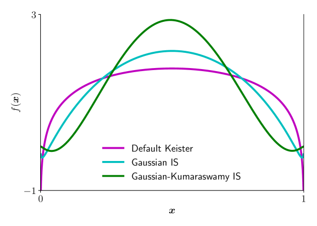
Figure 7: Keister functions with and without importance sampling (IS). Note that the Keister functions using importance sampling are generally less variable and therefore easier to integrate, as evidenced by the faster integration times.

9 Further Work

QMCPy is ripe for growth and development in several areas. We hope that the QMC community will join us in making this a reality.

Multi-level (quasi-)Monte Carlo (ML(Q)MC) methods make possible the computation of expectations of functionals of stochastic differential equations and partial differential equations with random coefficients. Such use cases appear in quantitative finance and geophysical applications. QMCPy’s ML(Q)MC’s capability is rudimentary, but under active development.

We hope to add a greater variety of use cases and are engaging collaborators to help. Sobol’ indices, partial differential equations with random coefficients, expected improvement measures for Bayesian optimization, and multivariate probabilities are some of those on our radar.

Recently, several QMC experts have focused on developing LD generators for Python. Well-established packages such as SciPy SCIPY and PyTorch PyTorch are have developed QMC modules that support numerous LD sequences and related functionalities. We plan to integrate the routines as optional backends for QMCPy’s LD generators. Creating ties to these other packages will allow users to call their preferred generators from within the QMCPy framework. Moreover, as features in QMCPy become more common and prove their value, we will try to incorporate them into SciPy and other popular, general-purpose packages.

We also plan to expand our library of digital net generating matrices. We wish to incorporate interlaced digital nets, polynomial lattices, and Niederreiter sequences, among others. By including high-quality defaults in QMCPy, we hope to make these sequences more readily available to the public.

Our DiscreteDistrution places equal weights on each support point, $\boldsymbol{X}_{i}$. In the future, we might generalize this to unequal weights.

QMCPy already includes importance sampling, but the choice of sampling distribution must be chosen a priori. We would like to see an automatic, adaptive choice following the developments of AsmGly2007a ; approx_zero_variance_simulation ; OweZho00a .

Control variates can be useful for QMC as well as for IID MC HicEtal03 . These should be incorporated into QMCPy in a seamless way.

We close with an invitation. Try QMCPy. If you find bugs or missing features, please submit an issue to https://github.com/QMCSoftware/QMCSoftware/issues. If you wish to add your great algorithm or use case, please submit a pull request to our GitHub repository at https://github.com/QMCSoftware/QMCSoftware/pulls. We hope that the community will embrace QMCPy.

- (1) Abadi, M., Agarwal, A., Barham, P., Brevdo, E., Chen, Z., Citro, C., Corrado, G.S., Davis, A., Dean, J., Devin, M., Ghemawat, S., Goodfellow, I., Harp, A., Irving, G., Isard, M., Jia, Y., Jozefowicz, R., Kaiser, L., Kudlur, M., Levenberg, J., Mané, D., Monga, R., Moore, S., Murray, D., Olah, C., Schuster, M., Shlens, J., Steiner, B., Sutskever, I., Talwar, K., Tucker, P., Vanhoucke, V., Vasudevan, V., Viégas, F., Vinyals, O., Warden, P., Wattenberg, M., Wicke, M., Yu, Y., Zheng, X.: TensorFlow: Large-scale machine learning on heterogeneous systems (2015). URL https://www.tensorflow.org/. Software available from tensorflow.org
- (2) Asmussen, S., Glynn, P.: Stochastic Simulation: Algorithms and Analysis, Stochastic Modelling and Applied Probability, vol. 57. Springer-Verlag, New York (2007). DOI 10.1007/978-0-387-69033-9
- (3) Bezanson, J., Karpinski, S., Shah, V.B., Edelman, A.: Julia: A fast dynamic language for technical computing. arXiv preprint arXiv:1209.5145 (2012)
- (4) Burkhardt, J.: Various software (2020). URL http://people.sc.fsu.edu/~jburkardt/
- (5) Choi, S.C.T., Ding, Y., Hickernell, F.J., Jiang, L., Jiménez Rugama, Ll.A., Li, D., Jagadeeswaran, R., Tong, X., Zhang, K., Zhang, Y., Zhou, X.: GAIL: Guaranteed Automatic Integration Library (versions 1.0–2.3.2). MATLAB software, http://gailgithub.github.io/GAIL\_Dev/ (2021). DOI 10.5281/zenodo.4018189
- (6) Choi, S.C.T., Hickernell, F.J., Jagadeeswaran, R., McCourt, M., Sorokin, A.: QMCPy: A quasi-Monte Carlo Python library (2020). DOI 10.5281/zenodo.3964489. URL https://qmcsoftware.github.io/QMCSoftware/
- (7) Choi, S.C.T., Hickernell, F.J., Jagadeeswaran, R., McCourt, M.J., Sorokin, A.: QMCPy documentation (2020). URL https://qmcpy.readthedocs.io/en/latest/
- (8) Cools, R., Kuo, F.Y., Nuyens, D.: Constructing embedded lattice rules for multivariate integration. SIAM Journal on Scientific Computing 28(6), 2162–2188 (2006). DOI 10.1137/06065074X
- (9) Darmon, Y., Godin, M., L’Ecuyer, P., Jemel, A., Marion, P., Munger, D.: LatNet builder (2018). URL https://github.com/umontreal-simul/latnetbuilder
- (10) Dick, J., Kuo, F., Sloan, I.H.: High dimensional integration — the Quasi-Monte Carlo way. Acta Numer. 22, 133–288 (2013). DOI 10.1017/S0962492913000044
- (11) Giles, M.: Multi-level (quasi-)Monte Carlo software (2020). URL https://people.maths.ox.ac.uk/gilesm/mlmc/
- (12) Google Inc.: TF Quant Finance: Tensorflow based Quant Finance Library (2021). URL https://github.com/google/tf-quant-finance
- (13) Harris, C.R., Millman, K.J., van der Walt, S.J., Gommers, R., Virtanen, P., Cournapeau, D., Wieser, E., Taylor, J., Berg, S., Smith, N.J., Kern, R., Picus, M., Hoyer, S., van Kerkwijk, M.H., Brett, M., Haldane, A., del Río, J.F., Wiebe, M., Peterson, P., Gérard-Marchant, P., Sheppard, K., Reddy, T., Weckesser, W., Abbasi, H., Gohlke, C., Oliphant, T.E.: Array programming with NumPy. Nature 585(7825), 357–362 (2020). DOI 10.1038/s41586-020-2649-2. URL https://doi.org/10.1038/s41586-020-2649-2
- (14) Hickernell, F.J., Choi, S.C.T., Jiang, L., Jiménez Rugama, L.A.: Monte Carlo simulation, automatic stopping criteria for. Wiley StatsRef: Statistics Reference Online pp. 1–7 (2014)
- (15) Hickernell, F.J., Sorokin, A.: Quasi-Monte Carlo (QMC) software in QMCPy Google Colaboratory notebook (2020). URL http://tinyurl.com/QMCPyTutorial
- (16) Hickernell, F.J., Sorokin, A.: Quasi-Monte Carlo (QMC) software in QMCPy Google Colaboratory notebook for MCQMC2020 article (2020). URL https://tinyurl.com/QMCPyArticle2021
- (17) Hickernell, F.J.: A generalized discrepancy and quadrature error bound. Math. Comp. 67, 299–322 (1998). DOI 10.1090/S0025-5718-98-00894-1
- (18) Hickernell, F.J.: Goodness-of-fit statistics, discrepancies and robust designs. Statist. Probab. Lett. 44, 73–78 (1999). DOI 10.1016/S0167-7152(98)00293-4
- (19) Hickernell, F.J., Jiang, L., Liu, Y., Owen, A.B.: Guaranteed conservative fixed width confidence intervals via Monte Carlo sampling. In: J. Dick, F.Y. Kuo, G.W. Peters, I.H. Sloan (eds.) Monte Carlo and Quasi-Monte Carlo Methods 2012, Springer Proceedings in Mathematics and Statistics, vol. 65, pp. 105–128. Springer-Verlag, Berlin (2013). DOI 10.1007/978-3-642-41095-6
- (20) Hickernell, F.J., Jiménez Rugama, Ll.A.: Reliable adaptive cubature using digital sequences. In: R. Cools, D. Nuyens (eds.) Monte Carlo and Quasi-Monte Carlo Methods: MCQMC, Leuven, Belgium, April 2014, Springer Proceedings in Mathematics and Statistics, vol. 163, pp. 367–383. Springer-Verlag, Berlin (2016). ArXiv:1410.8615 [math.NA]
- (21) Hickernell, F.J., Jiménez Rugama, Ll.A., Li, D.: Adaptive quasi-Monte Carlo methods for cubature. In: J. Dick, F.Y. Kuo, H. Woźniakowski (eds.) Contemporary Computational Mathematics — a celebration of the 80th birthday of Ian Sloan, pp. 597–619. Springer-Verlag (2018). DOI 10.1007/978-3-319-72456-0
- (22) Hickernell, F.J., Lemieux, C., Owen, A.B.: Control variates for quasi-Monte Carlo. Statist. Sci. 20, 1–31 (2005). DOI 10.1214/088342304000000468
- (23) Hofert, M., Lemieux, C.: qrng R package (2017). URL https://cran.r-project.org/web/packages/qrng/qrng.pdf
- (24) Jagadeeswaran, R., Hickernell, F.J.: Fast automatic Bayesian cubature using lattice sampling. Stat. Comput. 29, 1215–1229 (2019). DOI 10.1007/s11222-019-09895-9
- (25) Jagadeeswaran, R., Hickernell, F.J.: Fast automatic Bayesian cubature using Sobol’ sampling (2021+). In preparation for submission for publication
- (26) Jiménez Rugama, Ll.A., Hickernell, F.J.: Adaptive multidimensional integration based on rank-1 lattices. In: R. Cools, D. Nuyens (eds.) Monte Carlo and Quasi-Monte Carlo Methods: MCQMC, Leuven, Belgium, April 2014, Springer Proceedings in Mathematics and Statistics, vol. 163, pp. 407–422. Springer-Verlag, Berlin (2016). ArXiv:1411.1966
- (27) Keister, B.D.: Multidimensional quadrature algorithms. Computers in Physics 10, 119–122 (1996). DOI 10.1063/1.168565
- (28) Kucherenko, S.: BRODA (2020). URL https://www.broda.co.uk/index.html
- (29) Kumaraswamy, P.: A generalized probability density function for double-bounded random processes. Journal of Hydrology 46(1), 79–88 (1980). DOI 10.1016/0022-1694(80)90036-0
- (30) Kuo, F.Y., Nuyens, D.: Application of quasi-Monte Carlo methods to elliptic PDEs with random diffusion coefficients – a survey of analysis and implementation. Found. Comput. Math. 16, 1631–1696 (2016). URL https://people.cs.kuleuven.be/~dirk.nuyens/qmc4pde/
- (31) Lataniotis, C., Marelli, S., Sudret, B.: Uncertainty quantification in the cloud with UQCloud. In: 4th International Conference on Uncertainty Quantification in Computational Sciences and Engineering (UNCECOMP 2021), pp. 209–217 (2021)
- (32) L’Ecuyer, P.: SSJ: Stochastic Simulation in Java (2020). URL https://github.com/umontreal-simul/ssj
- (33) L’Ecuyer, P., Marion, P., Godin, M., Puchhammer, F.: A tool for custom construction of QMC and RQMC point sets. In: E. Arnaud, M. Giles, A. Keller (eds.) Monte Carlo and Quasi-Monte Carlo Methods: MCQMC, Oxford, 2020 (2021+)
- (34) L’Ecuyer, P., Munger, D.: Algorithm 958: Lattice Builder: A general software tool for constructing rank-1 latice rules. ACM Trans. Math. Software 42, 1–30 (2016)
- (35) L’Ecuyer, P., Tuffin, B.: Approximate zero-variance simulation. In: Proceedings of the 40th Conference on Winter Simulation, WSC ’08, p. 170–181. Winter Simulation Conference (2008)
- (36) Marelli, S., Sudret, B.: UQLab: A framework for uncertainty quantification in MATLAB. In: The 2nd International Conference on Vulnerability and Risk Analysis and Management (ICVRAM 2014), pp. 2554–2563. ASCE Library (2014). URL https://www.uqlab.com
- (37) Matoušek, J.: On the -discrepancy for anchored boxes. J. Complexity 14, 527–556 (1998)
- (38) Niederreiter, H.: Random Number Generation and Quasi-Monte Carlo Methods. CBMS-NSF Regional Conference Series in Applied Mathematics. SIAM, Philadelphia (1992)
- (39) Nuyens, D.: Magic point shop (2017). URL https://people.cs.kuleuven.be/~dirk.nuyens/qmc-generators/
- (40) OpenTURNS Developers: An open source initiative for the Treatment of Uncertainties, Risks ’N Statistics (2020). URL http://www.openturns.org
- (41) Owen, A.B.: Scrambling Sobol’ and Niederreiter–Xing points. Journal of Complexity 14(4), 466–489 (1998)
- (42) Owen, A.B.: On dropping the first Sobol’ point (2020). ArXiv:2008.08051 [math.NA]
- (43) Owen, A.B.: Randomized Halton sequences in R (2020). URL http://statweb.stanford.edu/~owen/code/
- (44) Owen, A.B.: About the R function: rsobol (2021). URL https://statweb.stanford.edu/~owen/reports/seis.pdf
- (45) Owen, A.B., Zhou, Y.: Safe and effective importance sampling. J. Amer. Statist. Assoc. 95, 135–143 (2000)
- (46) Paszke, A., Gross, S., Massa, F., Lerer, A., Bradbury, J., Chanan, G., Killeen, T., Lin, Z., Gimelshein, N., Antiga, L., Desmaison, A., Kopf, A., Yang, E., DeVito, Z., Raison, M., Tejani, A., Chilamkurthy, S., Steiner, B., Fang, L., Bai, J., Chintala, S.: PyTorch: An imperative style, high-performance deep learning library. In: H. Wallach, H. Larochelle, A. Beygelzimer, F. d'Alché-Buc, E. Fox, R. Garnett (eds.) Advances in Neural Information Processing Systems 32, pp. 8024–8035. Curran Associates, Inc. (2019). URL http://papers.neurips.cc/paper/9015-pytorch-an-imperative-style-high-performance-deep-learning-library.pdf
- (47) PyTorch Developers: PyTorch (2020). URL https://pytorch.org
- (48) Robbe, P.: Low discrepancy sequences in Julia (2020). URL https://github.com/PieterjanRobbe/QMC.jl
- (49) Robbe, P.: Multilevel Monte Carlo simulations in Julia (2021). URL https://github.com/PieterjanRobbe/MultilevelEstimators.jl
- (50) SciPy Developers: SciPy Ecosystem (2018). URL www.scipy.org
- (51) The MathWorks, Inc.: MATLAB R2021a. Natick, MA (2020)
- (52) Virtanen, P., Gommers, R., Oliphant, T.E., Haberland, M., Reddy, T., Cournapeau, D., Burovski, E., Peterson, P., Weckesser, W., Bright, J., van der Walt, S.J., Brett, M., Wilson, J., Millman, K.J., Mayorov, N., Nelson, A.R.J., Jones, E., Kern, R., Larson, E., Carey, C.J., Polat, İ., Feng, Y., Moore, E.W., VanderPlas, J., Laxalde, D., Perktold, J., Cimrman, R., Henriksen, I., Quintero, E.A., Harris, C.R., Archibald, A.M., Ribeiro, A.H., Pedregosa, F., van Mulbregt, P., SciPy 1.0 Contributors: SciPy 1.0: Fundamental Algorithms for Scientific Computing in Python. Nature Methods 17, 261–272 (2020). DOI 10.1038/s41592-019-0686-2