Experimental Tests of Invariant Set Theory

Abstract

We identify points of difference between Invariant Set Theory and standard quantum theory, and evaluate if these would lead to noticeable differences in predictions between the two theories. From this evaluation, we design a number of experiments, which, if undertaken, would allow us to investigate whether standard quantum theory or invariant set theory best describes reality.

I Introduction

For all the successes of modern physics over the last century-and-a-half, it has left us with three apparently incompatible branches - the nonlinear and deterministic General Relativity, the linear but indeterministic Quantum Theory, and the non-linear and deterministic, but uncomputable, Chaos Theory. For us to have a Theory of Everything, that describes all observed physical phenomena, we need a way to at least unite the first two, so we can describe physical phenomena at any scale. However, due to their differing takes on the determinacy of the universe, this has so far proved difficult.

Invariant Set Theory (IST) attempts to unify these three disparate branches by using insight from Chaos Theory to create a fully local and deterministic model of quantum phenomena [1, 2, 3, 4, 5, 6, 7, 8, 9, 10, 11, 12]. It does by assuming that the universe is a deterministic dynamical system evolving precisely on a fractal invariant set in state space. The natural metric to describe distances on a fractal set is the $p$-adic metric. This replaces the standard Euclidean metric of distance between states in state space. A consequence of this is that putative counterfactual states which lie in the fractal gaps of the invariant set are to be considered distant from states which do lie on the invariant set, even though from a Euclidean perspective such distances may appear small. Given the uncomputability of the possible states on any given fractal attractor, we cannot in advance distinguish states allowed and disallowed by this metric - hence, in IST, the appearance of randomness despite being deterministic.

$p$-adic numbers form a back-bone of modern number theory and as such provide a framework to describe quantum physics within a finite number-theoretic framework. An example is the notion of complementarity which underpins the uncertainty principle in quantum mechanics. In Invariant Set Theory complementarity is an emergent property of number theoretic properties of trigonometric functions such as $\cos{\phi}$, for example that $\cos\phi$ is not a rational number when $\exp{i\phi}$ is a primitive $p$th root of unity. The complex Hilbert Space of standard quantum mechanics arises is a singular limit of invariant set theory when $p$ is set equal to infinity.

However, despite showing how the vast majority of quantum phenomena can be described deterministically, the theory deviates from standard quantum physics in some of its predictions—mainly in ways which stem from the necessarily finiteness of the $p$-adic metric used. In this paper, we give these key points of deviation, and investigate the extent to which these could be used to experimentally test the theory.

II Entanglement Limits

In standard quantum theory, there is no limit to the number of quantum objects which can be maximally entangled - however, in IST, there is. Here, we codify this limit, and design experiments to test if it can be probed.

For this, we use the $M$-qubit W state [13, 14],

$$\left|W^{M}\right\rangle=\frac{1}{\sqrt{M}}\sum^{M-1}_{i=0}\left|0\right\rangle^{\otimes i}\left|1\right\rangle\left|0\right\rangle^{\otimes(M-1-i)}$$ (1)

(where $\left|\psi\right\rangle^{\otimes M}$ is the tensor product of $\left|\psi\right\rangle$ with itself $M$ times). For instance, the $M=3$ W state is

$$\left|W^{3}\right\rangle=\frac{\left|100\right\rangle+\left|010\right\rangle+\left|001\right\rangle}{\sqrt{3}}$$ (2)

The W state is a maximally entangled state of $M$ qubits—and in standard quantum theory, there is no limit to how high $M$ can be.

However, in IST, the large-but-finite dimension of the $p$-adic metric provides a limit - in this case to the number of qudits that can be maximally entangled. For multiple-qubit entanglement, this limit is codified in [11] as a maximum of $\log_{2}N$ qubits being able to be maximally entangled, in a $p$-adic system where the equatorial great circle of the Bloch sphere consists of $N$ equally-spaced discrete points.

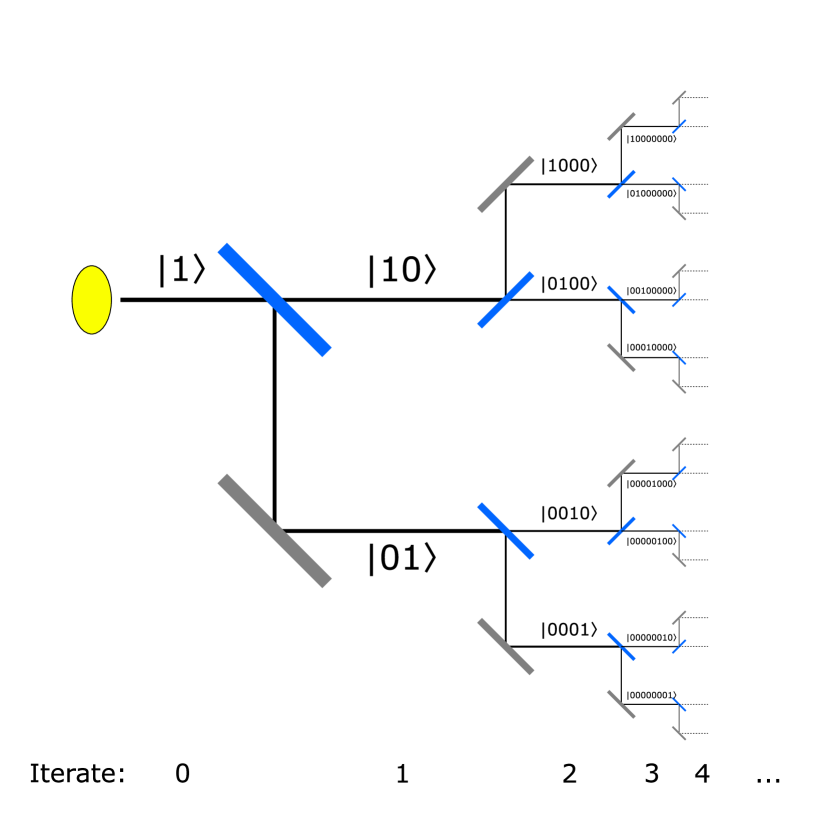
Figure 1: The first 4 iterates of a set-up to create the entangled state $\left|W^{M}\right\rangle$ (as given in Eq.1), where $M=2^{I}$ at the $I^{th}$ iterate. The diagonal blue lines are 50:50 beamsplitters, the diagonal grey lines mirrors, the yellow oval a single-photon source, and the black lines the possible paths of the photon. Given this maximally entangles $2^{I}$ qubits, IST predicts entanglement generated by an experiment like this should begin to fail after $I=\log_{2}\log_{2}N$ iterations, where the two spherical dimensions of the Bloch sphere are each $N$-discrete. We can test whether this entanglement holds or fails by putting mirrors at the ends of each path - if the photon returns with 100$\%$ probability to the input port, it was maximally entangled; if each beamsplitter splits it evenly, such that it only returns $2^{-I}$ of the time, the entanglement has decayed completely - return probabilities between show various levels of entanglement decay.

A system of maximally-entangled photon-vacuum qubits can be created using a single photon and a number of mirrors and 50:50 beamsplitters, as shown in Fig.1. This naturally forms a W state across $M$ qubits, and, by standard quantum theory, should potentially be able to be extended to $M\rightarrow\infty$. However, this disagrees with IST, which limits to a maximum of $M=\log_{2}N$ entangled qubits, where the two orthogonal spherical dimensions of the Bloch sphere ($\theta$ and $\phi$) are each discrete in $N$ divisions. While $p$ is expected to be very large, each qubit will only have been affected by $I=\log_{2}\log_{2}N$ beamsplitters, so, for realistic experimental beamsplitter loss of $0.1\%$, the chance of losing a given qubit to decoherence only reaches $1\%$ once the system has entangled over 1000 qubits, which is only possible by IST if $N\geq 10^{250}$. Further, an advantage of the W state is, even if decoherence effectively measures one of the qubits, so long as the result is 0 (the photon isn’t in that mode), this collapse leaves the remaining qubits still maximally entangled in the $(M-1)^{th}$ W state.

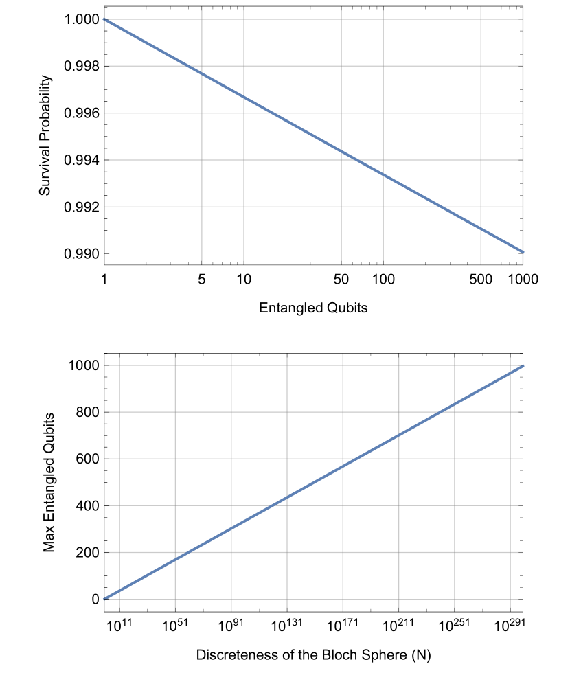
Figure 2: The survival probability of each qubit for a given set of entangled qubits created using the experiment in Fig.1, and the maximum number of entangled qubits that can be created in a version of IST where the $p$-adicity causes the Bloch sphere to be split into $N$ divisions in each angular direction. This shows how this beamsplitter experiment allows us to test this entanglement limit for very high-$p$ versions of IST, due to the comparative lack of loss-induced decoherence on the W state created.

Even if we obtain this state, we need to prove it is entangled. Gräfe et al [15] and Heilmann et al [16] have done this for 8 and 16 qubit W states respectively, confirming that they generated an entangled W state of that size (assuming they inputted a single photon), and Wang et al’s integrated silicon photonics chip could be used to do this for a 32-qubit W state [17]. It is an ongoing problem to specifically discern an entanglement-confirming optical layout for an arbitrarily-large W state, but Lougovski et al give the quantum-information-theoretical groundwork for doing so [18]. This involves using beamsplitters to shift the optical-path modes to instead each represent one possible permutation of phase combinations for the sub-components (ignoring the global phase of the state) - for instance, for the 4-qubit W state, combining beamsplitters after the state creation so as to have each final path act to project on one of the 4 states

$$\begin{split}\left|W_{1}^{4}\right\rangle=(\left|1000\right\rangle+\left|0100\right\rangle+\left|0010\right\rangle+\left|0001\right\rangle)/2\\ \left|W_{2}^{4}\right\rangle=(\left|1000\right\rangle-\left|0100\right\rangle-\left|0010\right\rangle+\left|0001\right\rangle)/2\\ \left|W_{3}^{4}\right\rangle=(\left|1000\right\rangle+\left|0100\right\rangle-\left|0010\right\rangle-\left|0001\right\rangle)/2\\ \left|W_{4}^{4}\right\rangle=(\left|1000\right\rangle-\left|0100\right\rangle+\left|0010\right\rangle-\left|0001\right\rangle)/2\end{split}$$ (3)

Doing this means a consistent detection on just one of the paths over meany runs (e.g. the one corresponding to just $\left|W_{1}^{4}\right\rangle$) indicates a pure entangled state is consistently being created (specifically here the state $\left|W_{1}^{4}\right\rangle$). Were the entanglement to break, the detections would begin to spread between the targeted state $\left|W_{1}^{4}\right\rangle$ and the other three states, until, for a maximally mixed state, each detector would click 25$\%$ of the time.

In the same way, for the $I^{th}$ iterate, consisting of $M=2^{I}$ qubits, there is a way (just using linear optical components) to project the eventual state into one of the $2^{I}$ phase permutations of $\left|W^{M}\right\rangle$, and so detect with certainty that a pure entangled state of $M$ qubits was created. Interestingly, preparing these states to certify entanglement requires each optical mode to again only interact with $I$ beamsplitters, to allow us to certify $M=2^{I}$-qubit entanglement, which simply squares the survival probability - meaning for 1000 qubits, it becomes $~{}98\%$ rather than $~{}99\%$. Again, given the resilience of the overall state to loss-induced decoherence, and the fact that Lougovski et al show this certification method also allows us to detect any entangled states of fewer than $M$ qubits, this loss probability poses very little issue to our test of IST - not to mention that, despite the loss, the total number of surviving (maximally-entangled) qubits tends to infinity as $I$ tends to infinity, rather than peaking at a certain value.

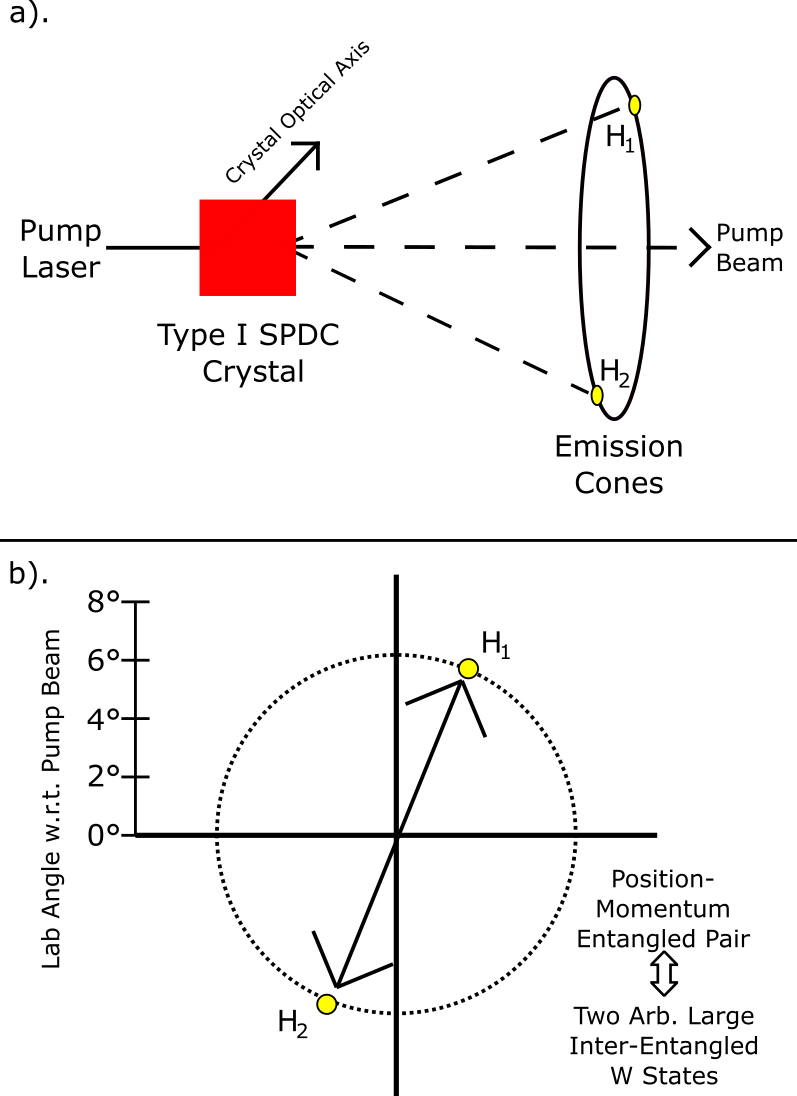
Figure 3: Type I spontaneous parametric downconversion source for the generation of pairs of position-and-momentum-entangled photons, as given by Rarity and Tapster [19]. The generated position of each photon on the cone can be viewed as a W state of arbitrary number of qubits $N$, and so the system of the two photons is a double-W state of $2N$ qubits. This arbitrary number of qubits $N$ can be lower-bounded as the resolution of a circular single-photon position detector array used to detect where on the circle each photon is emitted.

This W state-based experimental analysis of IST can be extended by looking at an experiment such as that given by Rarity and Tapster, where a pair of photons are generated in a cone of possible positions, with the angular position of one anti-correlated with the position of the other [19]. We show this in Fig.3. Considering just one photon in the cone, this is equivalent to a W state where $M$ is the number of sectors into which you subdivide the cone. Adding a second photon, position-entangled with the first, doubles the number of entangled qubits in the system.

Rarity and Tapster also give a way to prove these photons are entangled - by interfering them to violate a Bell inequality. However, as this is done assuming their position is a continuous variable, we need to adjust it to prove just how large it holds for as discrete variables.

This can be done by making a set of $2M$ apertures on the circumference of the cone, and splitting the ring into two half-circumferences. After this, similarly to what we do in Fig.1, we can iteratively combine adjacent apertures to get position-momentum entanglement between adjacent apertures, and, once this projects to equal superpositions across all $M$ apetures on each half-circle, record detected position for each half-circle’s photon. By comparing the final detected position between upper half-circumference and lower half-circumference, and seeing if they still correlate, we can confirm this double-W_M state.

While the phase between the upper photon and some other discrete division in the upper half will be random, it will be the same as the phase between the lower photon and some discrete division in the lower half. The correlation is always the same, but specific phases at different points on the circumference are not. This is why, using the two photons (and two split half-circles), we can prove the correlations still exist - a similar (though continuous) method was used by Rarity and Tapster to provably violate a Bell Inequality.

III No Continuous Variables

A second, related implication of IST is that it permits no continuous quantum variables. Due to the necessarily finite dimensions of the $p$-adic metric used in IST, the space of states allowed must also be finite. Given we can lower bound the number of states allowed as the dimension of the Hilbert space we use (to replicate classical information theory), we can say that, the existence of a qudit of dimension $d$ implies a state space of at least dimension $d$ (e.g. a qudit requires at least two distinct states: 0 and 1; a qutrit requires 3 states: 0, 1 and 2, etc…). Hardy extends this argument, saying that, to satisfy his axioms for quantum theory, between any two pure states in a system, there needs to be a continuous reversible transformation available on a system that goes from one to the other. To allow this, Hardy argues a qudit of dimension $d$ requires a state space of dimension $d^{2}$ [20].

This means for continuous variables to exist, given they have an infinite-dimensional Hilbert space [21], there must be an infinite number of states allowed - which is a violation of IST. Therefore, in IST, there can be no quantum continuous variables.

In standard quantum physics, a number of variables are held to be continuous - for instance, position, momentum, electric field strength, and time [22]. Therefore, for IST to hold true, all of these variables, currently thought continuous, would actually need to be discrete: of very high (but finite) dimension. While a number of theories/approaches hold one or another of these variables to be continuous (e.g. position in Loop Quantum Gravity, or time in certain toy models of the Universe), the idea that all previously-thought continuous variables are actually discrete would be controversial.

IV Gravity Is Inherently Decoherent

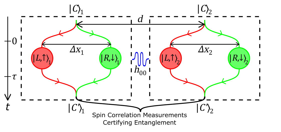
Figure 4: The experiment described by Bose et al [23], and separately by Marletto and Vedral [24], for testing the ability of gravity to entangle two masses. Two masses, $m_{i}$ for $i\in\{1,2\}$ are separated from each other by distance $d$. Both are initially in state $\left|C\right\rangle_{i}$, with embedded spin $(\left|\uparrow\right\rangle+\left|\downarrow\right\rangle)/\sqrt{2}$. They are then both admitted into Stern-Gerlach devices, which put them both into the spin-dependent superposition $(\left|L,\uparrow\right\rangle_{i}+\left|R,\downarrow\right\rangle_{i})/\sqrt{2}$, where $\left|L\right\rangle_{i}$ and $\left|R\right\rangle_{i}$ are separated from each other by distance $\Delta x_{i}$. They are left in these superpositions for time $\tau$, during which, if gravity is quantum-coherent, evolution under mutual gravitational attraction $h_{00}$ would entangle the two particles, adding relevant phases to both. After time $\tau$, an inverse Stern-Gerlach device is applied to each to return them both to their initial states (potentially modulo the phases applied by $h_{00}$). By applying this process, and measuring spin correlations between the two particles after each run, we can detect if relative phases have been applied to each, and so if gravity is coherent. For IST to hold, gravity must be decoherent, and so cannot entangle two masses, meaning no alteration of phases will be detected.

IST has been described as not so much a quantum theory of gravity (like String Theory and Loop Quantum Gravity), but a gravitational theory of the quantum [7]. Aside from its deterministic nature, nowhere is this more apparent than in how it views the regime where gravitational and quantum effects should both be present. In Invariant Set Theory, it is described as positing no gravitons and so no supersymmetry (spin-2 gravitons typically being seen as hinting at supersymmetry). Instead, it suggests that gravity is inherently decoherent, turning gravitationally-affected superpositions into maximally mixed states. IST also suggests that effects typically considered signs of dark matter/dark energy are instead due to the “smearing” of energy-momentum on space-times neighbouring $\mathcal{M}_{U}$ on $I_{U}$ influencing curvature of $\mathcal{M}_{U}$. This smearing avoids precise singularities in $\mathcal{M}_{U}$ - this avoidance being a key goal of many previous attempts to quantise General Relativity. However, Palmer admits in that paper that all of this still requires quantification. We attempt to begin this here.

Palmer suggests an alteration of the Einstein Field Equation (EFE) based on the presence and effects of possible universes $\mathcal{M}^{\prime}_{U}$ on our universe $\mathcal{M}_{U}$, leading to the equation instead being

$$\begin{split}G_{\mu\nu}&(\mathcal{M}_{U})=\\ &\frac{8\pi G}{c^{4}}\int_{\mathcal{N}(\mathcal{M}_{U})}T_{\mu\nu}(\mathcal{M}^{\prime}_{U})F(\mathcal{M}_{U},\mathcal{M}^{\prime}_{U})d\mu\end{split}$$ (4)

where $F(\mathcal{M}_{U},\mathcal{M}^{\prime}_{U})$ is some propagator to be determined and $d\mu$ is a suitably normalised Haar measure in some neighbourhood $\mathcal{N}(\mathcal{M}_{U})$ on $I_{U}$ [7]. Note this also sets the cosmological constant $\Lambda$ sometimes seen in the EFE to zero, given it separately resolves the issue of dark matter and the acceleration of the expansion of the universe.

This gravitational decoherence could be tested by experiments that involve putting heavy objects in spatial superpositions, allowing them to gravitationally interact, returning the spatial superposition components back to a single position, and seeing by the resulting interference pattern if there are any signs of entanglement between the objects (see Fig.4) [23, 24]. In this set-up, assuming gravity is coherent, the combined state of the two masses at different points in the experiment is

$$\begin{split}|\Psi&{}_{Init}\rangle_{12}=(\left|\uparrow\right\rangle_{1}+\left|\downarrow\right\rangle_{1})(\left|\uparrow\right\rangle_{2}+\left|\downarrow\right\rangle_{2})\left|C\right\rangle_{1}\left|C\right\rangle_{2}/2\\ |\Psi&(t=0)\rangle_{12}=(\left|L,\uparrow\right\rangle_{1}+\left|R,\downarrow\right\rangle_{1})(\left|L,\uparrow\right\rangle_{2}+\left|R,\downarrow\right\rangle_{2})/2\\ |\Psi&(t=\tau)\rangle_{12}=\frac{e^{i\phi}}{2}\Big{(}\left|L,\uparrow\right\rangle_{1}(\left|L,\uparrow\right\rangle_{2}+e^{i\Delta\phi_{LR}}\left|R,\downarrow\right\rangle_{2})\\ &+\left|R,\downarrow\right\rangle_{1}(e^{i\Delta\phi_{RL}}\left|L,\uparrow\right\rangle_{2}+\left|R,\downarrow\right\rangle_{2})\Big{)}\\ |\Psi&{}_{End}\rangle_{12}=\left|C^{\prime}\right\rangle_{1}\left|C^{\prime}\right\rangle_{2}=\Big{(}\left|\uparrow\right\rangle_{1}(\left|\uparrow\right\rangle_{2}+e^{i\Delta\phi_{LR}}\left|\downarrow\right\rangle_{2})\\ &+\left|\downarrow\right\rangle_{1}(e^{i\Delta\phi_{RL}}\left|\uparrow\right\rangle_{2}+\left|\downarrow\right\rangle_{2})\Big{)}\left|C\right\rangle_{1}\left|C\right\rangle_{2}/2\end{split}$$ (5)

where

$$\begin{split}&\Delta\phi_{LR}=\phi_{LR}-\phi,\;\Delta\phi_{RL}=\phi_{RL}-\phi\\ &\phi_{RL}\approx\frac{Gm_{1}m_{2}\tau}{\hbar(d-\Delta x)},\;\phi_{LR}\approx\frac{Gm_{1}m_{2}\tau}{\hbar(d+\Delta x)}\\ &\phi\approx\frac{Gm_{1}m_{2}\tau}{\hbar d}\end{split}$$ (6)

However, if gravity isn’t coherent, there are two possible final states: if gravity doesn’t also collapse the state, the final state will be equivalent to the initial one ($\left|\Psi_{Init}\right\rangle_{12}=\left|\Psi_{End}\right\rangle_{12}$); or, if gravity does collapse the superposition, each particle will be forced into the (spin) maximally mixed state

$$\left|\Psi_{MM}\right\rangle_{12}=\left|C\right\rangle\hskip-2.84526pt\left\langle C\right|_{i}(\left|\uparrow\right\rangle\hskip-2.84526pt\left\langle\uparrow\right|_{i}+\left|\downarrow\right\rangle\hskip-2.84526pt\left\langle\downarrow\right|_{i})/2$$ (7)

By measuring spin correlations to estimate the entanglement witness $\mathcal{W}=|\langle\sigma^{(1)}_{x}\otimes\sigma^{(2)}_{z}\rangle-\langle\sigma^{(1)}_{y}\otimes\sigma^{(2)}_{z}\rangle|$, we can distinguish the entangled state from the two other possible final states (if $\mathcal{W}>\mathbb{1}$, the state is entangled), and so see if gravity is coherent - for IST to hold, $\mathcal{W}$ needs to be less than or equal to $\mathbb{1}$.

V Conclusions

We have identified points of difference between Invariant Set Theory and standard quantum theory. While these are not fatal to IST, they provide potential avenues to experimentally test the theory, to see whether its deterministic, fractal-attractor-based structure is compatible with observed reality.