Quantum Monge–Kantorovich problem and transport distance between density matrices

Abstract

A quantum version of the Monge–Kantorovich optimal transport problem is analyzed. The transport cost is minimized over the set of all bipartite coupling states $\rho^{AB}$, such that both of its reduced density matrices $\rho^{A}$ and $\rho^{B}$ of dimension $N$ are fixed. We show that, selecting the quantum cost matrix to be proportional to the projector on the antisymmetric subspace, the minimal transport cost leads to a semidistance between $\rho^{A}$ and $\rho^{B}$, which is bounded from below by the rescaled Bures distance and from above by the root infidelity. In the single qubit case we provide a semi-analytic expression for the optimal transport cost between any two states and prove that its square root satisfies the triangle inequality and yields an analogue of the Wasserstein distance of order two on the set of density matrices. We introduce an associated measure of proximity of quantum states, called SWAP-fidelity, and discuss its properties and applications in quantum machine learning.

Introduction.—Remarkable progress in quantum technologies stimulates further research on foundations of quantum mechanics. In particular, one aims to improve our understanding of the structure of the set of quantum states BZ17 – the arena in which quantum information processing takes place. It is therefore important to analyze various distances in the space of quantum states and to describe their properties and diverse physical applications.

In the classical case one considers several distances in the space of probability distributions. A prominent role is played by the Monge distance, directly linked to the famous mass transport problem Mo1781 , in which one minimizes the work against friction required to move a pile of earth of shape $p^{A}$ into the final shape $p^{B}$. For continuous distributions the problem is solved analytically in any 1D case Sal43 and in several particular 2D cases RR98 , while effective numerical algorithms can be applied for any discrete probability distributions.

More general formulations of Kantorovich Kan42 ; Kan48 and Wasserstein Was69 , relying on joint probability distributions with marginals $p^{A}$ and $p^{B}$, are explicitly symmetric with respect to given probability distributions. Due to numerous applications of the mass transport problem in operations research and economics and its relation to the assignment problem, it remains a subject of intensive mathematical research Vi09 ; Ve13 . The transport problem was inspected from the perspective of free probability BV01 and applied in the study of causality EM17a ; EM17b ; EHMH20 .

An attempt to generalize the notion of the Monge distance for quantum theory was pursued for the setup of infinite ZS98 and finite dimensional ZS01 ; BZ17 Hilbert spaces. Such a distance between any two quantum states, defined by the Monge distance between the corresponding Husimi distributions, enjoys the semiclassical property: the distance between two coherent states, centered at points $x$ and $y$ in the classical phase space, is equal to the distance, $|x-y|$, between the points at which both coherent states are concentrated. This property, crucial for studies on quantum analogues of the Lyapunov exponent ZWS93 , is also shared by the distance recently proposed in WWW20 .

Any definition based on the notion of the Husimi function depends on the choice of the set of coherent states. It is therefore natural to look for a universal method to introduce the transport distance between quantum states directly by applying the Kantorovich–Wasserstein approach and performing optimization over the set of bipartite quantum states with fixed marginals AF17 ; GP18 ; CGT18 . In spite of recent vibrant activity in this field GMT16 ; CGNT17 ; BGJ19 ; FGZ19 ; CGGT17 ; Fri20 ; Du20b , this aim has not been fully achieved until now YZYY18 ; Reira18 ; Ikeda20 ; PMTL20 .

In parallel, the quantum optimal transport has found numerous applications in quantum physics, in particular in connection with the measures of proximity of quantum states DPT19 ; CM20 ; DR20 ; CGP20 . The latter play a key role in quantum metrology BC94 ; Sa17 ; LYLW20 , as well as in quantum machine learning QML ; LW18 ; Wu19 ; KdPMLL21 .

In this work we introduce a measure of proximity of quantum states, dubbed the “SWAP-fidelity”, as it is inspired by the quantum optimal transport with a specific quantum cost matrix. It shares many properties with the standard Uhlmann–Jozsa fidelity Uh76 ; Jo94 and agrees with the latter if at least one of the states is pure. We prove that the square root of the associated quantum optimal transport cost yields a new distance on the space of qubits which is a quantum analogue of the Wasserstein-2 distance. For larger dimensions we show analytically that this quantity gives a semidistance, bounded from above by the root infidelity and from below by the rescaled Bures distance. We further discuss the general form of a quantum cost matrix and study the quantum-to-classical transition of the transport problem. The latter shows that the quantum optimal transport is cheaper than the classical one, generalizing the results of CGP20 . Finally, we discuss an application of the new quantum metric in the context of quantum generative adversarial networks.

Classical transport problem.—To formulate the mass transport problem in the setup of Kantorovich for any probability distributions $p^{A}_{i}$ and $p^{B}_{j}$ one introduces the notion of a classical coupling – a joint probability distribution $P^{AB}_{ij}$ with two specified marginals, $p^{A}_{i}=\sum_{j}P^{AB}_{ij}$ and $p^{B}_{j}=\sum_{i}P^{AB}_{ij}$. In the case of two probability vectors of order $N$, $p^{A},p^{B}\in\Delta_{N}$, any joint distribution $P^{AB}\in\Delta_{N^{2}}$, which determines a transport plan, is represented by a single vector $P_{\mu}$, with $\mu=(i-1)N+j=1,\dots,N^{2}$. The set $\Gamma^{cl}(p^{A},p^{B})$ of all admissible couplings forms a convex subset of the simplex $\Delta_{N^{2}}$, with extreme points characterized in Pa07 .

Consider a set of $N$ points $X\vcentcolon=\{x_{i}\}_{i=1}^{N}$ equipped with a distance function $d$. With the latter we associate a symmetric $N\times N$ matrix $E_{ij}\vcentcolon=d(x_{i},x_{j})$. Assuming that the transport cost of a unit of mass from point $x_{i}$ to point $x_{j}$ is equal to the distance $E_{ij}$, one can formulate the classical transport problem RR98 ; Fri20 . In order to study its quantum analogue it will be convenient to reshape the square distance matrix $E_{ij}$ of dimension $N$ into a distance vector $D_{\mu}$ of length $N^{2}$.

To generate a Wasserstein distance between probability distributions $p^{A}$ and $p^{B}$ one can use a $N^{2}\times N^{2}$ classical cost matrix $C$ which is diagonal, $C_{\mu\nu}=D_{\mu}\delta_{\mu\nu}$ for $\mu,\nu=1,\dots,N^{2}$, and a diagonal density matrix $\rho^{AB}_{\mu\nu}=P_{\mu}\delta_{\mu\nu}$. For a given transport plan $P^{AB}$ and some parameter $p\geq 1$ the total transport cost is given by the scalar product, ${\hat{T}}_{C,p}(P)\vcentcolon=\sum_{\mu=1}^{N^{2}}(D_{\mu})^{p}P_{\mu}=\Tr\,C^{p}\rho^{AB}$. The minimal transport cost, $T_{C,p}^{cl}\vcentcolon=\min_{P}{\hat{T}}_{C,p}(P)$, optimized for a given value of the parameter $p$, leads to the family of Wasserstein distances,

$$\!\!W^{cl}_{C,p}(p^{A},p^{B})\vcentcolon=\Bigl{(}\min_{P^{AB}\in\Gamma^{cl}}(\Tr\,C^{p}\rho^{AB})\Bigr{)}^{\!1/p}\!=\big{(}T_{C,p}^{cl}\big{)}^{1/p}.$$ (1)

The minimum is taken over the set $\Gamma^{cl}(p^{A},p^{B})$ of classical couplings RR98 . If $d(x_{i},x_{j})=1-\delta_{ij}$, the space $X$ has the geometry of an $N$-point simplex $\Delta_{N}$. In this case, $C^{p}=C$ and $W^{cl}_{C,p}=(W^{cl}_{C,1})^{1/p}$ for any $p\geq 1$, so we shall abbreviate $T^{cl}\vcentcolon=T_{C,p}^{cl}$ and denote the classical cost matrix by $C^{cl}$.

Proximity of quantum states.—We now switch to the quantum setting and denote the set of $N\times N$ density matrices by $\Omega_{N}=\{\rho:\ \rho=\rho^{\dagger},\ \rho\geq 0,\ \Tr\rho=1\}$. To quantify the closeness of any two quantum states one uses various distances on $\Omega_{N}$ – see BZ17 . The trace distance, singled out by the Helstrom theorem on optimal distinguishability Helstrom , reads $D_{\rm Tr}(\rho^{A},\rho^{B})\vcentcolon=\frac{1}{2}{\rm{Tr}}|\rho^{A}-\rho^{B}|$, where $|X|:=\sqrt{XX^{\dagger}}$. Another way to characterise the proximity between two density matrices relies on Uhlmann–Jozsa fidelity Uh76 ; Jo94 , $F(\rho^{A},\rho^{B}):=\big{(}{\rm{Tr}}|\sqrt{\rho^{A}}\sqrt{\rho^{B}}|\big{)}^{2}$. It leads to the following distances: the root infidelity GLN05 , $I\vcentcolon=\sqrt{1-F}$, the Bures distance Uh76 ; Uh95 , $B\vcentcolon=\sqrt{2(1-\sqrt{F})}$, and the Bures angle, $A\vcentcolon=\tfrac{2}{\pi}\arccos\sqrt{F}$. Note that the Bures distance and other distances based on fidelity are closely related to statistical distinguishability and quantum Fisher information BC94 ; Sa17 , so they have a direct interpretation in quantum metrology LYLW20 .

We shall now introduce a quantity analogous to fidelity, which is directly related to the quantum optimal transport problem and its applications in machine learning Wu19 .

SWAP-fidelity.— Consider two arbitrary states $\rho^{A},\rho^{B}\in\Omega_{N}$. A composed (bipartite) density matrix $\rho^{AB}$ of order $N^{2}$ is called a coupling matrix Wi15 between $\rho^{A}$ and $\rho^{B}$ if both partial traces agree, $\Tr_{A}\rho^{AB}=\rho^{B}$ and $\Tr_{B}\rho^{AB}=\rho^{A}$. The set of all possible quantum couplings matrices will be denoted by $\Gamma^{Q}(\rho^{A},\rho^{B})\subset\Omega_{N^{2}}$ – see Fig.1c. The bipartite quantum states can be conveniently represented in the Fano form – see Supplemental Material (SM).

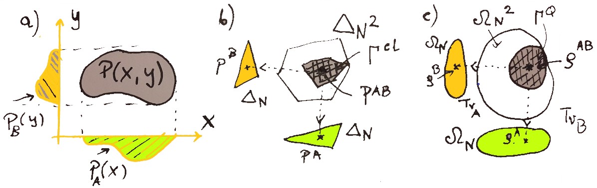
Figure 1: Couplings between probability distributions used for Kantorovich distance: a) continuous 1D probabilities $p_{A}(x)$ and $p_{B}(y)$ coupled by a joint distribution $P(x,y)$; b) two $N$-point classical states $p^{A},p^{B}\in\Delta_{N}$ coupled by a joint state $P^{AB}\in\Gamma^{cl}\subset\Delta_{N^{2}}$ with adjusted marginals; c) two quantum states $\rho^{A},\rho^{B}\in\Omega_{N}$ coupled by a bipartite state $\rho^{AB}\in\Gamma^{Q}\subset\Omega_{N^{2}}$ such that $\Tr_{A}\rho^{AB}=\rho^{B}$ and $\Tr_{B}\rho^{AB}=\rho^{A}$.

Let $S$ denote the SWAP operator, $S(|x\rangle\otimes|y\rangle):=|y\rangle\otimes|x\rangle$ for any vectors $|x\rangle$ and $|y\rangle$. For any $\rho^{A},\rho^{B}\in\Omega_{N}$ we introduce the SWAP-fidelity:

$$F_{S}(\rho^{A},\rho^{B})\vcentcolon=\max_{\rho^{AB}\in\Gamma^{Q}}\big{(}\Tr\,S\,\rho^{AB}\big{)},$$ (2)

where the maximum is taken over the set $\Gamma^{Q}$ of all admissible coupling matrices $\rho^{AB}$.

Proposition 1. For any dimension $N$, the SWAP-fidelity $F_{S}$ is a symmetric jointly concave function from $\Omega_{N}\times\Omega_{N}$ to the unit interval. Furthermore, $F_{S}(\rho^{A},\rho^{B})=1$ iff $\rho^{A}=\rho^{B}$, $F_{S}(\rho^{A},\rho^{B})=0$ iff  $\Tr\rho^{A}\rho^{B}=0$, and

$$F_{S}\bigl{(}\rho^{A},\rho^{B}\bigr{)}=F_{S}\bigl{(}U\rho^{A}U^{\dagger},U\rho^{B}U^{\dagger}\bigr{)},\text{ for }\,U\in\mathrm{U}(N),$$ (3)

$$F(\rho^{A},\rho^{B})\leq F_{S}(\rho^{A},\rho^{B})\leq\sqrt{F(\rho^{A},\rho^{B})},$$ (4)

$$F_{S}\bigl{(}\rho^{A}\otimes\sigma^{A},\rho^{B}\otimes\sigma^{B}\bigr{)}\geq F_{S}\bigl{(}\rho^{A},\rho^{B}\bigr{)}F_{S}\bigl{(}\sigma^{A},\sigma^{B}\bigr{)}.$$ (5)

The above result, proven in SM, shows that, in analogy to the fidelity $F$, the SWAP-fidelity $F_{S}$ equals unity iff both states coincide and vanishes iff they are orthogonal. Furthermore, it interpolates between fidelity and root fidelity – see Ineq. (4) – with the first inequality saturated if at least one of the states is pure. Notably, the SWAP-fidelity is super-multiplicative with respect to tensor product as it satisfies inequality (5) characteristic to superfidelity MPHUZ . Note also that $F_{S}$ is jointly concave, as is the root fidelity $\sqrt{F}$, while it has a probabilistic interpretation for pure states, $F_{S}(\phi,\psi)=F(\phi,\psi)=|\langle\phi,\psi\rangle|^{2}$ – see BZ17 . The SWAP-fidelity is shown below to be closely related to the quantum optimal transport and yields a novel metric on the Bloch ball.

Quantum cost matrix.— To study the transport problem between two quantum states of order $N$ we need to specify a quantum cost matrix $C^{Q}$ of size $N^{2}$. Let $\{{|i\rangle}\}_{i=1}^{N}$ be the computational basis of an $N$-level quantum system and denote the maximally entangled singlet states in the subspace spanned by $|i\rangle$ and $|j\rangle$ by $|\psi^{-}_{ij}\rangle=\frac{1}{\sqrt{2}}(|i,j\rangle-|j,i\rangle)$. In the case of the simplex geometry, $E_{ij}=1-\delta_{ij}$, the quantum optimal transport enjoys several desirable features if one chooses the cost matrix $C^{Q}$ to be the projector onto the antisymmetric subspace,

$$C^{Q}=\sum_{j>i=1}^{N}|\psi^{-}_{ij}\rangle\langle\psi^{-}_{ij}|=\tfrac{1}{2}({\mathbbm{1}}_{N^{2}}-S)=(C^{Q})^{2},$$ (6)

as advocated also in YZYY18 ; Reira18 ; Wu19 ; Du20b . In particular, for the simplest, one-qubit problem, $N=2$, the cost matrix reads

$$C^{Q}=\frac{1}{2}\left[\begin{array}[]{llll}0&\ 0&\ 0&0\\ 0&\ 1&\!\!\!-1&0\\ 0&\!\!\!-1&\ 1&0\\ 0&\ 0&\ 0&0\end{array}\right]=|\psi^{-}\rangle\langle\psi^{-}|$$ (7)

The above quantum cost matrix $C^{Q}$ of size $N^{2}$ forms a coherification KCPZ18 of a classical cost matrix $C^{cl}={\rm diag}(C^{Q})$ corresponding to the simplex geometry.

We are now going to look for the minimal quantum transport cost, which can be expressed using the SWAP-fidelity:

$$T^{Q}(\rho^{A},\rho^{B})\vcentcolon=\min_{\rho^{AB}\in\Gamma^{Q}}\big{(}\Tr\,C^{Q}\rho^{AB}\big{)}=\frac{1-F_{S}(\rho^{A},\rho^{B})}{2}.$$ (8)

Proposition 1 directly implies that for any two states $\rho^{A},\rho^{B}\in\Omega_{N}$ the optimal quantum transport cost, $T^{Q}$, is jointly convex, symmetric, non-negative and vanishes iff $\rho^{A}=\rho^{B}$. Furthermore, for $C^{Q}$ given by (6) one has

$$T^{Q}\bigl{(}\rho^{A},\rho^{B}\bigr{)}=T^{Q}\bigl{(}U\rho^{A}U^{\dagger},U\rho^{B}U^{\dagger}\bigr{)},$$ (9)

for any unitary operator $U$ on $\mathbb{C}^{N}$. Hence, $T^{Q}$ forms a semidistance on $\Omega_{N}$, as shown independently in Wu19 . In analogy with the classical definition (1), for any $p\geq 0$ we introduce a quantum analogue of the $p$-Wasserstein distance, $W_{p}\vcentcolon=(T^{Q})^{1/p}$. As shown below, $W_{2}$ plays a distinguished role, so we will denote it simply by $W\vcentcolon=W_{2}$.

As an immediate corollary of Ineq. (4), proven in SM with help of recent results by Yu et al. YZYY18 , we arrive at explicit bounds for the quantum transport cost and its square root $W$.

Corollary 2. For any two states $\rho^{A},\rho^{B}\in\Omega_{N}$ we have

$$\!\!\!\!\!\tfrac{1}{\sqrt{2}}B(\rho^{A},\rho^{B})\geq\tfrac{1}{\sqrt{2}}I(\rho^{A},\rho^{B})\geq W(\rho^{A},\rho^{B})\geq\tfrac{1}{2}B(\rho^{A},\rho^{B}).$$ (10)

Furthermore, the second inequality is saturated if either $\rho^{A}$ or $\rho^{B}$ is pure.

Single qubit transport.—In the simplest case of $N=2$ the quantum cost matrix is given by (7). As shown in SM the full solution of the quantum transport problem for the one-qubit case is equivalent to solving a polynomial equation of order six. The latter yields analytic expressions in several special cases.

For two diagonal matrices, $\rho^{cl}_{r}={\rm\operatorname{diag}}(r,1-r)$ and $\rho^{cl}_{s}={\rm\operatorname{diag}}(s,1-s)$, we have

$$W\big{(}\rho^{cl}_{r},\;\rho^{cl}_{s}\big{)}=\tfrac{1}{\sqrt{2}}\max\big{\{}\big{|}\sqrt{r}-\sqrt{s}\big{|},\big{|}\sqrt{1-r}-\sqrt{1-s}\big{|}\big{\}}.$$ (11)

Furthermore, if one of the states is totally mixed we obtain,

$$W\bigl{(}\tfrac{1}{2}{\mathbbm{1}},\rho\bigr{)}=\tfrac{1}{2}\max\big{\{}\big{|}1-\sqrt{2\lambda}\big{|},\big{|}1-\sqrt{2(1-\lambda)}\big{|}\big{\}},$$ (12)

where $\lambda$ and $1-\lambda$ denote the eigenvalues of $\rho$. A surprisingly simple formula is available for two isospectral states,

$$W\bigl{(}\rho,\;U\rho U^{\dagger}\bigr{)}=\sqrt{\tfrac{1}{\sqrt{2}}-\sqrt{\lambda(1-\lambda)}}\;\big{|}\sin(\theta/2)\big{|},$$ (13)

where $\{\lambda,1-\lambda\}$ is the common spectrum and $\theta$ is the $U$-dependent angle between Bloch vectors associated with the states – see SM. In the case of a single qubit we obtain one of the key results of this work, proved in SM.

Theorem 3. For $N=2$ the function $W_{p}$ satisfies the triangle inequality iff $p\geq 2$: for any states $\rho^{A},\rho^{B},\rho^{C}\in\Omega_{2}$ one has $W_{p}(\rho^{A},\rho^{B})+W_{p}(\rho^{B},\rho^{C})\geq W_{p}(\rho^{A},\rho^{C})$. Thus, $W_{p}$ generates a distance on the Bloch ball $\Omega_{2}$, analogous to the classical $p$-Wasserstein distance (1), provided that $p\geq 2$.

Numerical studies carried out for the simplex geometry with $N=3$ and $4$ allow us to conjecture that $W_{p}$ is actually a distance on $N$-level systems for any $N$ and $p\geq 2$. Whereas the quantum transport cost itself, $T^{Q}=W_{1}$, is not a distance on $\Omega_{2}$, its square root, $W_{2}$, is – see SM. Note that, similarly, while the infidelity $1-F$ does not satisfy the triangle inequality, its square root, $I=\sqrt{1-F}$, does GLN05 . An analogous property was recently proved for the quantum Jensen–Shannon divergence, the square root of which satifies the triangle inequality and leads to the transmission metric BH09 ; Vi19 .

Recall also that the Monge distance between quantum states defined by the Husimi distribution with respect to spin coherent states for $N=2$ leads to the Hilbert–Schmidt distance and the Euclidean geometry on the Bloch ball, while the discrete Monge distance, describing movements of the Majorana stars corresponding to pure states, gives geodesic distance on the Bloch sphere ZS01 . Whereas formula (10) implies that $W$ is strongly equivalent to the Bures metric $B$ and induces the same topology on the Bloch ball, the corresponding (curved) geometries are different. This is illustrated in Fig. 2 for a fixed mixed state $\rho^{A}$ and $\rho^{B}$ varying continuously from $\rho^{A}$ to the pure state ${|+\rangle}$. We witness the validity of the bound (10), with $W(\rho^{A},{|+\rangle})=I(\rho^{A},{|+\rangle})$. Observe also that initially the transport distance curve closely follows that of the Bures distance. Using the Pauli matrices, $\sigma_{i}$, and the Bloch representation, $\rho_{\pm}(\vec{\tau})\vcentcolon=\tfrac{1}{2}\left({\mathbbm{1}}\pm\vec{\tau}\cdot\vec{\sigma}\right)$ for $\|\vec{\tau}\|\in[0,1]$, we have

$$W\bigl{(}\rho_{+}(\vec{\tau}),\rho_{-}(\vec{\tau}\bigr{)}=\tfrac{1}{\sqrt{2}}B\bigl{(}\rho_{+}(\vec{\tau}),\rho_{-}(\vec{\tau})\bigr{)}.$$ (14)

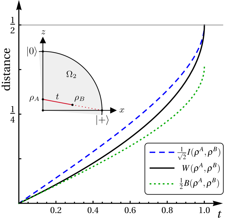
Figure 2: Bounds (10) illustrated in the Bloch ball $\Omega_{2}$. The distances between the state $\rho^{A}=\tfrac{9}{20}{\mathbbm{1}}+\tfrac{1}{10}{|0\rangle}{\langle 0|}$ and $\rho^{B}=(1-t)\rho^{A}+t({|+\rangle}{\langle+|})$ are shown as a function of $t\in[0,1]$ varying along the Euclidean line (red line in the inset).

Another insight into the geometry induced by the transport distance $W$ is gained by the study of geodesics – trajectories in the space of states – on which the triangle inequality is saturated for every triple of points. Such geodesics do not exist for either the root infidelity or for the Bures distance. On the other hand, the geodesics of the Bures angle metric $A$ exist and have a nice geometrical interpretation Uhlmann as great circles on the Uhlmann 3-hemisphere $\tfrac{1}{2}S^{3}$. When projected onto the equatorial plane they form ellipses within the real (i.e. $y=0$) slice of the Bloch ball. Interestingly, such geodesics also exist for the transport metric $W$, though their shape is more complex, as shown in Fig. 3.

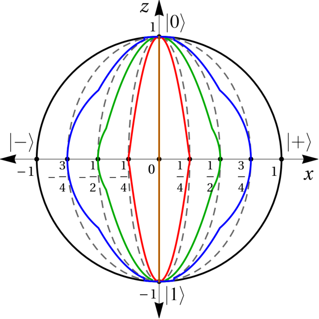
Figure 3: The $y=0$ section of the Bloch ball $\Omega_{2}$. Solid colored curves represent the geodesics of the transport metric $W$, while dashed lines are ellipses corresponding to the geodesics of the Bures angle $A$.

Quantization of an arbitrary classical cost matrix.—In a more general set-up consider an arbitrary distance function on the $N$-point set $X$, determined by the matrix $E_{ij}$. With any such classical geometry of $X$ we associate the following quantum cost matrix

$$C^{Q}_{E}=\sum_{j>i=1}^{N}E_{ij}|\psi^{-}_{ij}\rangle\langle\psi^{-}_{ij}|.$$ (15)

Accordingly, for any $p\geq 1$ we define

$$T^{Q}_{E,p}(\rho^{A},\rho^{B})\vcentcolon=\min_{\rho^{AB}\in\Gamma^{Q}}\big{(}\Tr\,(C^{Q}_{E})^{p}\rho^{AB}\big{)}, W_{E,p}\vcentcolon=\big{(}T^{Q}_{E,p}\big{)}^{1/p}$$

and prove the following result in SM.

Proposition 4. For any $N$, any $p\geq 1$, and any choice of classical geometry $E$, the $p$^th root of the corresponding optimal quantum transport cost, $W_{E,p}$, is a semidistance on $\Omega_{N}$.

The quantum-to-classical transition.—It is instructive to compare the quantum transport problem with its classical counterpart. To this end one embeds classical probability vectors in diagonal density matrices. The following result shows that the quantum transport cost between two classical states is always cheaper than the corresponding classical cost (see also CGP20 ).

Proposition 5. Let $\vec{r},\vec{s}$ be two $N$-dimensional probability vectors and let $\rho^{cl}_{\vec{r}},\rho^{cl}_{\vec{s}}\in\Omega_{N}$ be the corresponding quantum states defined as $(\rho^{cl}_{\vec{r}})_{ij}\vcentcolon=r_{i}\delta_{ij}$. Then,

$$T^{Q}\bigl{(}\rho^{cl}_{\vec{r}},\rho^{cl}_{\vec{s}}\bigr{)}\ \leq\ T^{cl}\bigl{(}\vec{r},\vec{s}\bigr{)}.$$

This follows from the fact that the quantum optimization is performed over a strictly larger set of admissible couplings, $\Gamma^{cl}(\vec{r},\vec{s})\subset\Gamma^{Q}(\rho^{cl}_{\vec{r}},\rho^{cl}_{\vec{s}})$.

The quantum-to-classical transition of the transport problem can be interpreted in terms of decoherence caused by the interaction of the information processing device with its environment. As a simple model (cf. Zurek03 ) one can assume that the quantum cost matrix is acted upon by a dephasing channel $\mathcal{E}_{\alpha}(C^{Q})=\alpha C^{Q}+(1-\alpha)\operatorname{diag}(C^{Q})$, with the parameter $\alpha\in[0,1]$ proportional to the $l_{1}$-coherence BCP14 . One can then study the function $T^{Q}_{\alpha}\vcentcolon=\min_{\rho^{AB}\in\Gamma^{Q}}\big{(}\Tr\,\mathcal{E}_{\alpha}(C^{Q})\rho^{AB}\big{)}$. In the single-qubit case it is easy to check (see SM) that $\sqrt{T^{Q}_{\alpha}}$ is a distance on the set of commuting density matrices of order 2. Moreover, it is a strictly decreasing function of $\alpha$, provided that the two input states are different and none of them is pure.

Applications.—The introduced SWAP-fidelity offers an original measure of proximity between quantum states and thus provides a new tool to quantify protocols of quantum information processing. Its most promising and straightforward application pertains to quantum generative adversarial networks (QGANs) LW18 ; DdK18 . This protocol of quantum machine learning QML consists of a generator, which produces “fake” data, and a discriminator, which aims at distinguishing between the real and fake input data. The adversarial training reaches a fixed point when the generator produces data with true statistics and the discriminator’s efficiency is 50%. Similar to with classical GANs, the choice of the distance between real and fake data is critical for the stability and performance of the training WGAN ; Wu19 ; LYLW20 . In LYLW20 it was argued that problems with efficiency of quantum learning algorithms PT11 ; MBSBN18 ; WFCSSCC20 ; CSVCC21 arise because the employed measure of proximity diminishes exponentially with the number of qubits. Although the introduced SWAP-fidelity suffers from the same drawback for pure states (as it equals to fidelity in this case), it might prove superior for mixed states because of its super-multiplicativity (5).

In fact, in Wu19 a QGAN based on the semidistance $T^{Q}$ was shown to exhibit improved performance over other QGANs. Furthermore, it is noise tolerant and can be successfully used to approximate complicated quantum circuits with a limited number of quantum gates. Our results suggest that the choice $W=\sqrt{T^{Q}}$ is superior to $T^{Q}$, as it forms a genuine distance.

Outlook and conclusions.— We studied the quantum transport problem for density matrices of dimension $N$ with a cost matrix $C^{Q}$ taken to be a projector onto the antisymmetric subspace. In the case of any two single-qubit states we presented a constructive procedure to compute the quantum transport cost. A more detailed mathematical study is presented in the companion paper CEFZ21 .

Inspired by the Wasserstein distance of order $2$, we proved that the square root of the optimal transport cost, $W_{2}=\sqrt{T^{Q}}$, yields a distance on the Bloch ball, bounded by the rescaled Bures distance and the root infidelity. In the general problem of $N$-level systems and arbitrary classical geometry $E$ we showed that an analog of the $p$-Wasserstein distance $W_{p}$ yields a semidistance on the full space of quantum states for any $p\geq 1$. Furthermore, numerical results allow us to conjecture that $\sqrt{W_{1}}$ enjoys the triangle inequality in full generality.

Given the multifarious applications of the classical Wasserstein distances, we expect its quantum analogue to play a pivotal role in diverse branches of quantum information processing. Furthermore, the SWAP-fidelity – a novel quantity introduced in this work – is likely to offer new advances in characterizing proximity between quantum states.

Acknowledgements.—It is a pleasure to thank W. Słomczyński for inspiring discussions and helpful remarks. Financial support by Simons collaboration grant for mathematicians, Narodowe Centrum Nauki under the Maestro grant number DEC-2015/18/A/ST2/00274 and by Foundation for Polish Science under the Team-Net project no. POIR.04.04.00-00-17C1/18-00 is gratefully acknowledged.

Appendix A Properties of the quantum optimal transport

In this section we provide some details about the general quantum optimal transport problem, along with the proof of Proposition 4 from this article. For a complete mathematically oriented presentation of the problem the reader is invited to consult the companion-article CEFZ21 .

Let $\mathcal{H}=\mathbb{C}^{N}\otimes\mathbb{C}^{N}$ for some $N\geq 2$. The SWAP operator $S$ is a linear operator on $\mathcal{H}$, which acts on product states as $S(|x\rangle\otimes|y\rangle)=|y\rangle\otimes|x\rangle=\vcentcolon{|y,x\rangle}$. Since $S^{2}=\mathbbm{1}_{N^{2}}$ and $S=S^{\dagger}$ its eigenvalues are $\pm 1$. The Hilbert space $\mathcal{H}$ thus admits an orthogonal decomposition $\mathcal{H}=\mathcal{H}_{S}\oplus\mathcal{H}_{A}$ into symmetric and antisymmetric subspaces $\mathcal{H}_{S}$ and $\mathcal{H}_{A}$, respectively. The former can be identified with the symmetric complex matrices of order $N^{2}$, while the latter with the skew-symmetric ones.

Definition A1. A $N^{2}\times N^{2}$ complex matrix $C$ is called a quantum cost matrix if it is positive semidefinite, and $C\,X=0$ if and only if the support of $X$ equals to $\mathcal{H}_{S}$.

Explicit examples of quantum cost matrices are provided by formula (15) in the main body of the article. Note also that if $C$ is a quantum cost matrix, then so is $C^{p}$ for any $p>0$.

Definition A2. Let $C$ be a quantum cost matrix of dimension $N^{2}$. The associated quantum transport cost is a map $T^{Q}_{C}:\Omega_{N}\times\Omega_{N}\to\mathbb{R}$ defined as

$$T^{Q}_{C}(\rho^{A},\rho^{B})\;\;\vcentcolon=\min_{\rho^{AB}\in\Gamma^{Q}(\rho^{A},\rho^{B})}\big{(}\Tr\,C\,\rho^{AB}\big{)},$$ (16)

with the set of quantum couplings

$$\Gamma^{Q}(\rho^{A},\rho^{B})=\{\rho^{AB}\in\Omega_{N^{2}}\;|\;\Tr_{A}\rho^{AB}=\rho^{B},\Tr_{B}\rho^{AB}=\rho^{A}\}.$$

Proposition A3. For any quantum cost matrix $C$, $T^{Q}_{C}$ is a convex function on $\Omega_{N}\times\Omega_{N}$.

Proof.

Let $\rho^{A},\rho^{B},\sigma^{A},\sigma^{B}\in\Omega_{N}$ and let $a\in[0,1]$. Assume that $\rho^{AB}\in\Gamma^{Q}(\rho^{A},\rho^{B})$ and $\sigma^{AB}\in\Gamma^{Q}(\sigma^{A},\sigma^{B})$ are the optimal quantum couplings, i.e.

$$T^{Q}_{C}(\rho^{A},\rho^{B})=\Tr\,C\,\rho^{AB}, T^{Q}_{C}(\sigma^{A},\sigma^{B})=\Tr\,C\,\sigma^{AB}.$$

Define, for any $a\in[0,1]$, $\tau^{AB}\vcentcolon=a\rho^{AB}+(1-a)\sigma^{AB}$. Then, $\tau^{AB}\in\Gamma^{Q}\big{(}a\rho^{A}+(1-a)\sigma^{A},a\rho^{B}+(1-a)\sigma^{B}\big{)}$ and

$$T^{Q}_{C}(a\rho^{A}+(1-a)\sigma^{A},a\rho^{B}+(1-a)\sigma^{B})\\ \leq\Tr\,C\,\tau^{AB}=aT^{Q}_{C}(\rho^{A},\rho^{B})+(1-a)T^{Q}_{C}(\sigma^{A},\sigma^{B}).$$ (17)

∎

The following central result implies Proposition 4 from the main text, because $C^{Q}_{E}$ are quantum cost matrices, and if $T^{Q}_{C}$ is a semidistance then so is $(T^{Q}_{C})^{1/p}$ for any $p\geq 0$.

Theorem A4. Let $C$ be a $N^{2}\times N^{2}$ quantum cost matrix. Then $T^{Q}_{C}$ is a semidistance on the space of $N$-level quantum systems $\Omega_{N}$.

Proof.

We need to show that, for any $\rho^{A},\rho^{B}\in\Omega_{N}$,

1. $T^{Q}_{C}(\rho^{A},\rho^{B})\geq 0$,

2. $T^{Q}_{C}(\rho^{A},\rho^{B})=0$ if and only iff $\rho^{B}=\rho^{A}$,

3. $T^{Q}_{C}(\rho^{A},\rho^{B})=T^{Q}_{C}(\rho^{B},\rho^{A})$.

(i) Note that because $C$ is positive semidefinite and any $\rho^{AB}\in\Gamma^{Q}$ is a state in $\Omega_{N^{2}}$, we have $\Tr\,C\,\rho^{AB}\geq 0$. Hence, $T_{C}^{Q}(\rho^{A},\rho^{B})\geq 0$ for any $\rho^{A},\rho^{B}\in\Omega_{N}$.

(ii) Suppose first that $\rho^{A}=\rho^{B}=\rho$. Given its spectral decomposition $\rho=\sum_{i=1}^{N}\sqrt{\lambda_{i}}{|i\rangle}{\langle i|}$ we take the purification of $\rho$:

$$\rho^{\text{pur}}\vcentcolon=\sum_{i,j=1}^{N}\sqrt{\lambda_{i}\lambda_{j}}{|i\rangle}{|i\rangle}{\langle j|}{\langle j|}.$$

Clearly, $\rho^{\text{pur}}\in\Gamma^{Q}(\rho,\rho)$. Since ${|i\rangle}{|i\rangle}\in\mathcal{H}_{S}$ we have, by definition of the quantum cost matrix, $C\big{(}{|i\rangle}{|i\rangle}\big{)}=0$. Consequently, $\Tr C\rho^{\text{pur}}=0$ and $T^{Q}_{C}(\rho,\rho)=0$.

Suppose now, conversely, that $T^{Q}_{C}(\rho^{A},\rho^{B})=0$. This implies that $\Tr C\rho^{AB}=0$ for some $\rho^{AB}\in\Gamma^{A}(\rho^{A},\rho^{B})$. Consider its spectral decomposition $\rho^{AB}=\sum_{i=1}^{N^{2}}\mu_{i}{|X_{i}\rangle}{\langle X_{i}|}$, where ${|X_{i}\rangle}$ are vectors in $\mathcal{H}$. We have ${\langle X_{i}|}C{|X_{i}\rangle}=0$ for any $i$, which means that ${|X_{i}\rangle}\in\mathcal{H}_{S}$. But this implies that $\Tr_{A}\rho^{AB}=\Tr_{B}\rho^{AB}$, and hence $\rho^{A}=\rho^{B}$.

(iii) A general state in $\Gamma^{Q}(\rho^{A},\rho^{B})\subset\Omega_{N^{2}}$ can be decomposed in an orthonormal basis as follows

$$\rho^{AB}=\sum_{i,j,k,\ell}c_{ijk\ell}{|i\rangle}{|j\rangle}{\langle k|}{\langle\ell|}.$$ (18)

Consequently, we have

$$\rho^{A} =\Tr_{B}\rho^{AB}=\sum_{i,j,k}c_{ijkj}{|i\rangle}{\langle k|},$$

$$\rho^{B} =\Tr_{A}\rho^{AB}=\sum_{j,k,\ell}c_{kjk\ell}{|j\rangle}{\langle\ell|}.$$

Now, the SWAP operator extends to the space $\Omega_{N^{2}}$ and acts on the basis vector as follows:

$$S\big{(}{|i\rangle}{|j\rangle}{\langle k|}{\langle\ell|}\big{)}=S\big{(}{|i\rangle}{|j\rangle}\big{)}{\langle k|}{\langle\ell|}={|j\rangle}{|i\rangle}{\langle k|}{\langle\ell|}.$$

Hence, we have

$$S\rho^{AB}S^{\dagger}=\sum_{i,j,k,\ell}c_{ijk\ell}{|j\rangle}{|i\rangle}{\langle\ell|}{\langle k|}.$$

Consequently,

$$\Tr_{B}S\rho^{AB}S^{\dagger} =\sum_{j,k,\ell}c_{kjk\ell}{|j\rangle}{\langle\ell|}=\rho^{B},$$

$$\Tr_{A}S\rho^{AB}S^{\dagger} =\sum_{i,j,k}c_{ijkj}{|i\rangle}{\langle k|}\,\,=\,\rho^{A}.$$

Hence, $S\rho^{AB}S^{\dagger}=\vcentcolon\rho^{BA}\in\Gamma^{Q}(\rho^{B},\rho^{A})=S\,\Gamma^{Q}(\rho^{A},\rho^{B})S^{\dagger}$. Recall that $\mathcal{H}_{S},\mathcal{H}_{A}$ are invariant subspaces of $S$ corresponding to the eigenvalues $1$ and $-1$, respectively. As $C\mathcal{H}_{S}=0$ and $C\mathcal{H}_{A}\subset\mathcal{H}_{A}$, it follows that $SC=CS=-C$, and thus $SCS^{\dagger}=C$. Finally, we have

$$T^{Q}_{C}(\rho^{A},\rho^{B}) =\min_{\rho^{AB}\in\Gamma^{Q}(\rho^{A},\rho^{B})}\big{(}\Tr\,C\,\rho^{AB}\big{)}$$

$$=\min_{\rho^{AB}\in\Gamma^{Q}(\rho^{A},\rho^{B})}\big{(}\Tr\,S\,C\,S^{\dagger}\,S\,\rho^{AB}S^{\dagger}\big{)}$$

$$=\min_{\rho^{BA}\in\Gamma^{Q}(\rho^{B},\rho^{A})}\big{(}\Tr\,C\,\rho^{BA}\big{)}=T^{Q}_{C}(\rho^{B},\rho^{A}). \Box$$

∎

Proposition A5. Let $U,V\in\mathrm{U}(N)$ be unitary transformations and let $C^{\prime}\vcentcolon=(U\otimes V)C(U^{\dagger}\otimes V^{\dagger})$. Then, for any $\rho^{A},\rho^{B}\in\Omega_{N}$,

$$T^{Q}_{C}\bigl{(}\rho^{A},\rho^{B}\bigr{)}=T^{Q}_{C^{\prime}}\bigl{(}U\rho^{A}U^{\dagger},V\rho^{B}V^{\dagger}\bigr{)}.$$ (19)

Proof.

Using the representation (18) of $\rho^{AB}$ we quickly deduce that

$$(U\otimes V)\rho^{AB}(U^{\dagger}\otimes V^{\dagger})\\ =\sum_{i,j,k,\ell}c_{ijk\ell}(U{|i\rangle})(V{|j\rangle})({\langle k|}U^{\dagger})({\langle\ell|}V^{\dagger}).$$

This implies that

$$\Tr_{A}\;(U\otimes V)\rho^{AB}(U^{\dagger}\otimes V^{\dagger})=V\rho^{B}V^{\dagger},$$

$$\Tr_{B}\;(U\otimes V)\rho^{AB}(U^{\dagger}\otimes V^{\dagger})=U\rho^{A}U^{\dagger},$$

which proves

$$(U\otimes V)\,\Gamma^{Q}(\rho^{A},\rho^{B})(U^{\dagger}\otimes V^{\dagger})\subset\Gamma^{Q}(U\rho^{A}U^{\dagger},V\rho^{B}V^{\dagger}).$$

Similarly, one shows

$$(U^{\dagger}\otimes V^{\dagger})\,\Gamma^{Q}(U\rho^{A}U^{\dagger},V\rho^{B}V^{\dagger})(U\otimes V)\subset\Gamma^{Q}(\rho^{A},\rho^{B}).$$

Hence,

$$(U\otimes V)\Gamma^{Q}(\rho^{A},\rho^{B})(U^{\dagger}\otimes V^{\dagger})=\Gamma^{Q}(U\rho^{A}U^{\dagger},V\rho^{B}V^{\dagger}).$$

Now, because

$$\Tr\,C\,\rho^{AB}=\Tr\,(U\otimes V)C(U^{\dagger}\otimes V^{\dagger})(U\otimes V)\rho^{AB}(U^{\dagger}\otimes V^{\dagger})$$

we obtain

$$T^{Q}_{C}(\rho^{A},\rho^{B}) =\min_{\rho^{AB}\in\Gamma^{Q}(\rho^{B},\rho^{A})}\big{(}\Tr\,C\,\rho^{AB}\big{)}$$

$$=\min_{\rho^{AB}\in\Gamma^{Q}(\rho^{A},\rho^{B})}\big{(}\Tr\,C^{\prime}\,(U\otimes V)\rho^{AB}(U^{\dagger}\otimes V^{\dagger})\big{)}$$

$$=\min_{\sigma^{AB}\in\Gamma^{Q}(U\rho^{A}U^{\dagger},V\rho^{B}V^{\dagger})}\big{(}\Tr\,C^{\prime}\,\sigma^{AB}\big{)}$$

$$=T^{Q}_{C^{\prime}}(U\rho^{A}U^{\dagger},V\rho^{B}V^{\dagger}). \Box$$

∎

Formula (9) announced in the article is a simple consequence of Proposition A4.

Corollary A6. The optimal quantum transport cost with the cost matrix $C^{Q}=\tfrac{1}{2}\big{(}\mathbbm{1}_{N^{2}}-S\big{)}$ is unitarily invariant:

$$T^{Q}\bigl{(}\rho^{A},\rho^{B}\bigr{)}=T^{Q}\bigl{(}U\rho^{A}U^{\dagger},U\rho^{B}U^{\dagger}\bigr{)},$$ (20)

for any $U\in\mathrm{U}(N)$.

Proof.

Observe that the cost matrix $C^{Q}$ is unitarily invariant, $(U\otimes U)C^{Q}(U^{\dagger}\otimes U^{\dagger})=C$. Hence the result follows from Proposition A4 with $V=U$. ∎

Appendix B Bounds for the optimal quantum cost

In this Section we prove the inequalities (10) in the main body of the article based on the results of YZYY18 .

Let $\rho^{A}$, $\rho^{B}$ be any two states in $\Omega_{N}$. Theorem 10 in YZYY18 yields

$$\tfrac{1+F(\rho^{A},\rho^{B})}{2}\leq\max_{\rho^{AB}\in\Gamma^{Q}}\Tr(\tfrac{1}{2}({\mathbbm{1}}_{N^{2}}+S)\rho^{AB})\leq\tfrac{1+\sqrt{F(\rho^{A},\rho^{B})}}{2},$$ (21)

where $S$ is the SWAP operator. Because $C^{Q}=\tfrac{1}{2}\big{(}\mathbbm{1}_{N^{2}}-S\big{)}$ we have

$$2T^{Q}(\rho^{A},\rho^{B})=2\!\!\min_{\rho^{AB}\in\Gamma^{Q}}\big{(}\Tr\,C^{Q}\rho^{AB}\big{)}=1-\max_{\rho^{AB}\in\Gamma^{Q}}\big{(}\Tr\,S\rho^{AB}\big{)}.$$

Hence, from formula (21) we deduce that

$$\frac{1-\sqrt{F(\rho^{A},\rho^{B})}}{2}\leq T^{Q}(\rho^{A},\rho^{B})\leq\frac{1-F(\rho^{A},\rho^{B})}{2}.$$

Furthermore,

$$1-F(\rho^{A},\rho^{B}) =\left(1-\sqrt{F(\rho^{A},\rho^{B})}\right)\left(1+\sqrt{F(\rho^{A},\rho^{B})}\right)$$

$$\leq 2\left(1-\sqrt{F(\rho^{A},\rho^{B})}\right).$$

After taking the square root of the above inequalities we obtain the desired bounds (10).

We now prove yet another inequality and the last statement of Corollary 2.

Proposition B1. For any two states $\rho^{A},\rho^{B}\in\Omega_{N}$ we have,

$$T^{Q}(\rho^{A},\rho^{B})\leq\tfrac{1}{2}\big{(}1-\Tr\rho^{A}\rho^{B}\big{)}.$$ (22)

Moreover, if either $\rho^{A}$ or $\rho^{B}$ is pure then

$$W(\rho^{A},\rho^{B})=\tfrac{1}{\sqrt{2}}I(\rho^{A},\rho^{B})=\tfrac{1}{\sqrt{2}}\sqrt{1-\Tr\rho^{A}\rho^{B}}.$$ (23)

Proof.

First observe that $\rho^{A}\otimes\rho^{B}\in\Gamma^{Q}(\rho^{A},\rho^{B})$, which implies $T^{Q}(\rho^{A},\rho^{B})\leq\Tr C^{Q}(\rho^{A}\otimes\rho^{B})$. Now, the well-known identity $\Tr S(\rho^{A}\otimes\rho^{B})=\Tr\rho^{A}\rho^{B}$ (see Wer89 ; MPHUZ ) yields

$$\Tr({\mathbbm{1}}_{N^{2}}-S)(\rho^{A}\otimes\rho^{B})=1-\Tr\rho^{A}\rho^{B},$$

and formula (22) follows.

To prove the second formula we use the fact that if one of the states $\rho^{A}$, $\rho^{B}$ is pure, then $\Gamma^{Q}(\rho^{A},\rho^{B})=\{\rho^{A}\otimes\rho^{B}\}$ (as explained in FGZ19 and CEFZ21 ). In such a case the inequality (22) is hence saturated.

The middle part of (23) follows from the known property of the fidelity, $F({|\psi\rangle}{\langle\psi|},\sigma)=\Tr{|\psi\rangle}{\langle\psi|}\sigma={\langle\psi|}\sigma{|\psi\rangle}$. ∎

For the sake of completeness, let us also recall the Fuchs–van de Graaf inequality FvG99 , which relates the quantum fidelity to the trace distance, $D$. For any $\rho^{A},\rho^{B}\in\Omega_{N}$,

$$1-\sqrt{F(\rho^{A},\rho^{B})}\leq D(\rho^{A},\rho^{B})\leq\sqrt{1-F(\rho^{A},\rho^{B})}.$$ (24)

This inequality, combined with Ineq. (10) from the main text, implies that, for any $\rho^{A},\rho^{B}\in\Omega_{N}$,

$$W(\rho^{A},\rho^{B})\leq\sqrt{D(\rho^{A},\rho^{B})}.$$

Appendix C SWAP-fidelity

In this section we provide the complete proof of Proposition 1, which is based on the general results included in Section A.

For any $N$ the SWAP-fidelity, $F_{S}$, is a function on $\Omega_{N}\times\Omega_{N}$ defined as follows:

$$F_{S}(\rho^{A},\rho^{B})\vcentcolon=\max_{\rho^{AB}\in\Gamma^{Q}(\rho^{A},\rho^{B})}\big{(}\Tr\,S\,\rho^{AB}\big{)}.$$

Proposition C1. For any two states $\rho^{A},\rho^{B}\in\Omega_{N}$ we have

$$a)\quad F_{S}(\rho^{A},\rho^{B})=F_{S}(\rho^{B},\rho^{A}),$$

$$b)\quad 0\leq\Tr\rho^{A}\rho^{B}\leq F_{S}(\rho^{A},\rho^{B})\leq 1,$$

$$c)\quad F_{S}(\rho^{A},\rho^{B})=1\text{ iff }\rho^{A}=\rho^{B},$$

$$d)\quad F_{S}(\rho^{A},\rho^{B})=0\text{ iff }\Tr\rho^{A}\rho^{B}=0,$$

$$e)\quad F_{S}\bigl{(}a\rho^{A}+(1-a)\sigma^{A},a\rho^{B}+(1-a)\sigma^{B}\bigr{)}\geq$$

$$\quad\geq\,aF_{S}\bigl{(}\rho^{A},\rho^{B}\bigr{)}+(1-a)F_{S}\bigl{(}\sigma^{A},\sigma^{B}\bigr{)},\,\text{ for }a\in[0,1],$$

$$f)\quad F_{S}\bigl{(}\rho^{A},\rho^{B}\bigr{)}=F_{S}\bigl{(}U\rho^{A}U^{\dagger},U\rho^{B}U^{\dagger}\bigr{)},\text{ for }\,U\in\mathrm{U}(N),$$

$$g)\quad F(\rho^{A},\rho^{B})\leq F_{S}(\rho^{A},\rho^{B})\leq\sqrt{F(\rho^{A},\rho^{B})},$$

$$h)\quad F_{S}\bigl{(}\rho^{A}\otimes\sigma^{A},\rho^{B}\otimes\sigma^{B}\bigr{)}\geq F_{S}\bigl{(}\rho^{A},\rho^{B}\bigr{)}F_{S}\bigl{(}\sigma^{A},\sigma^{B}\bigr{)}.$$

Proof.

By definition (16) we have, after setting $C=C^{Q}$, $F_{S}=1-2T^{Q}$. Consequently, points $a)$ and $c)$ follow from Theorem A4, points $(iii)$ and $(ii)$, respectively. Similarly, point $f)$ is an immediate consequence of Corollary A6, while $e)$ follows from Proposition A3, since if $T^{Q}$ is convex, then $2T^{Q}$ is convex and $F_{S}=1-2T^{Q}$ is concave. Point $b)$ follows from Theorem A4 point (i) and inequality (22). Now, point $g)$ is a straightforward implication of Ineqs. (21) proven in YZYY18 . Then, point $d)$ follows from an analogous property of the quantum fidelity Jo94 .

Finally, let us address point $h)$. As previously, we set $\rho^{AB}\in\Gamma^{Q}(\rho^{A},\rho^{B})$, $\sigma^{AB}\in\Gamma^{Q}(\sigma^{A},\sigma^{B})$ to be the optimal quantum couplings

$$F_{S}(\rho^{A},\rho^{B})=\Tr\,S\,\rho^{AB}, F_{S}(\sigma^{A},\sigma^{B})=\Tr\,S\,\sigma^{AB}.$$

Now, define the following bipartite state

$$\tau^{AB}=U(\rho^{AB}\otimes\sigma^{AB})U^{\dagger},$$

with $U:\mathcal{H}^{A}\otimes\mathcal{H}^{B}\otimes\mathcal{H}^{A}\otimes\mathcal{H}^{B}\to\mathcal{H}^{A}\otimes\mathcal{H}^{A}\otimes\mathcal{H}^{B}\otimes\mathcal{H}^{B}$ being a reshuffling operator, which acts as $U=\mathrm{id}\otimes S\otimes\mathrm{id}$. Having chosen an orthonormal basis of $\mathcal{H}^{A}\otimes\mathcal{H}^{B}$ we write

$$\rho^{AB} =\sum r_{abcd}\,{|a\rangle}{|b\rangle}{\langle c|}{\langle d|},$$

$$\sigma^{AB} =\sum s_{e\!f\!gh}\,{|e\rangle}{|f\rangle}{\langle g|}{\langle h|},$$

where the summation is over all relevant indices. Then,

$$\tau^{AB} =\sum r_{abcd}\,s_{e\!f\!gh}\,{|a\rangle}{|e\rangle}{|b\rangle}{|f\rangle}{\langle c|}{\langle g|}{\langle d|}{\langle h|}.$$

Tracing over the subsystem $A$ yields

$$\Tr_{A}\tau^{AB} =\sum r_{abcd}\,s_{e\!f\!gh}\,\delta_{ac}\,\delta_{eg}\,{|b\rangle}{|f\rangle}{\langle d|}{\langle h|}$$

$$=\sum r_{abad}\,s_{e\!f\!eh}\,{|b\rangle}{|f\rangle}{\langle d|}{\langle h|}=\rho^{B}\otimes\sigma^{B}.$$

Analogously, one shows that $\Tr_{B}\tau^{AB}=\rho^{A}\otimes\sigma^{A}$, hence $\tau^{AB}\in\Gamma^{Q}(\rho^{A}\otimes\sigma^{A},\rho^{B}\otimes\sigma^{B})$. For such a coupling we have

$$\Tr S\tau^{AB} =\Tr\,\sum r_{abcd}\,s_{e\!f\!gh}\,{|b\rangle}{|f\rangle}{|a\rangle}{|e\rangle}{\langle c|}{\langle g|}{\langle d|}{\langle h|}$$

$$=\sum r_{abba}\,s_{e\!f\!f\!e}=\big{(}\Tr S\rho^{AB}\big{)}\big{(}\Tr S\sigma^{AB}\big{)}$$

$$=F_{S}\bigl{(}\rho^{A},\rho^{B}\bigr{)}F_{S}\bigl{(}\sigma^{A},\sigma^{B}\bigr{)}.$$

Since $\Tr S\tau^{AB}\leq F_{S}\bigl{(}\rho^{A}\otimes\sigma^{A},\rho^{B}\otimes\sigma^{B}\bigr{)}$, point $h)$ follows. ∎

Appendix D Single-qubit transport problem: general case

The key result in the single-qubit transport problem with cost matrix $C^{Q}=\tfrac{1}{2}\big{(}{\mathbbm{1}}_{4}-S\big{)}$ is the following:

Theorem D1. For any $\rho^{A},\rho^{B}\in\Omega_{2}$ we have

$$T^{Q}(\rho^{A},\rho^{B})=\max_{U\in\mathrm{U}(2)}\;\frac{1}{2}\left(\sqrt{(U^{\dagger}\rho^{A}U)_{11}}-\sqrt{(U^{\dagger}\rho^{B}U)_{11}}\,\right)^{2},$$ (25)

where $\rho_{11}$ denotes the upper-left entry of a $2\times 2$ matrix $\rho$.

The complete proof presented in CEFZ21 relies on the fact that rank of an extreme point $\rho^{AB}\in\Gamma^{Q}(\rho^{A},\rho^{B})$ is always at most 2 for $\rho^{A},\rho^{B}\in\Omega_{2}$ and the equivalence of the original quantum transport problem to the so-called “dual problem” (see also Wu19 ):

Proposition D2. Let $\rho^{A},\rho^{B}\in\Omega_{N}$ and let $C$ be any quantum cost matrix. Then,

$$\!\!\!\!\!\!T_{C}^{Q}(\rho^{A},\rho^{B})=\sup\Big{\{}\Tr\big(\sigma^{A}\rho^{A}+\sigma^{B}\rho^{B}\big{missing})\;\Big{|}\;\sigma^{A},\sigma^{B}\in\mathrm{H}_{N},\\ C-\sigma^{A}\otimes\mathbbm{1}_{N}-\mathbbm{1}_{N}\otimes\sigma^{B}\geq 0\Big{\}},$$

where $\mathrm{H}_{N}$ denotes the set of Hermitian $N\times N$ matrices. If $\rho^{A}$ and $\rho^{B}$ are positive definite then the supremum is achieved.

We now introduce a convenient notation for qubits in the $y=0$ section of the Bloch ball. Let $O$ denote the rotation matrix

$$O(\theta)=\begin{bmatrix}\cos(\theta/2)&-\sin(\theta/2)\\ \sin(\theta/2)&\cos(\theta/2)\end{bmatrix},\quad\text{for }\theta\in[0,2\pi),$$

and using the Pauli matrices $\sigma_{i}$ define, for $r\in[0,1]$,

$$\rho(r,\theta) \vcentcolon=O(\theta)\begin{bmatrix}r&0\\ 0&1-r\end{bmatrix}O(\theta)^{\top}$$

$$\,=(2r-1)\big{(}\sin\theta\sigma_{1}+\cos\theta\sigma_{3}\big{)}.$$

Because of unitary invariance (20), the quantum transport problem between two arbitrary qubits $\rho^{A},\rho^{B}\in\Omega_{2}$ can be reduced to the case $\rho^{A}=\rho(s,0)$ and $\rho^{B}=\rho(r,\theta)$, with three parameters, $s,r\in[0,1]$ and $\theta\in[0,2\pi)$. The parameter $\theta$ is the angle between the Bloch vectors associated with $\rho^{A}$ and $\rho^{B}$. With such a parametrization we can further simplify the single-qubit transport problem.

Observe first that if $s\in\{0,1\}$ then $\rho^{A}$ is pure, and if $r\in\{0,1\}$ then $\rho^{B}$ is pure. In any such case an explicit solution of the qubit transport problem is given by formula (23).

Theorem D3. Let $\rho^{A}=\rho(s,0),\rho^{B}=\rho(r,\theta)$ and assume that $0<r,s<1$. Then

$$T^{Q}(\rho^{A},\rho^{B})=$$ (26)

$$\!\!\max_{\phi\in\Phi(s,r,\theta)}\tfrac{1}{4}\big{(}\sqrt{1+(2s-1)\cos\phi}-\sqrt{1+(2r-1)\cos(\theta+\phi)}\big{)}^{2},$$

where $\Phi(s,r,\theta)$ is the set of all $\phi$ satisfying the equation

$$\frac{(2s-1)^{2}\sin^{2}\phi}{1+(2s-1)\cos\phi}=\frac{(2r-1)^{2}\sin^{2}(\theta+\phi)}{1+(2r-1)\cos(\theta+\phi)}.$$ (27)

Furthermore, the set $\Phi(s,r,\theta)$ has at most 6 elements.

Proof.

A unitary $2\times 2$ matrix $U$ can be parametrized, up to a global phase, with three angles $\alpha,\beta,\phi\in[0,2\pi)$,

$$U=\begin{bmatrix}e^{i\alpha}&0\\ 0&e^{-i\alpha}\end{bmatrix}O(\phi)\begin{bmatrix}e^{i\beta}&0\\ 0&e^{-i\beta}\end{bmatrix}.$$

We thus have

$$\!\!(U^{\dagger}\rho(r,\theta)U)_{11}=\vcentcolon f(r,\theta;\alpha,\phi)=$$

$$\quad\tfrac{1}{2}\Big{(}1+(2r-1)\big{(}\cos(\theta)\cos(\phi)+\cos(2\alpha)\sin(\theta)\sin(\phi)\big{)}\Big{)}.$$

This quantity does not depend on the parameter $\beta$, so we can set $\beta=0$. Note also that $f(s,0;\alpha,\phi)$ does not depend on $\alpha$. With $\rho^{A}=\rho(s,0),\rho^{B}=\rho(r,\theta)$, Theorem D1 yields

$$T^{Q}(\rho^{A},\rho^{B})=\max_{\alpha,\phi\in[0,2\pi)}\Big{(}\sqrt{f(s,0;0,\phi)}-\sqrt{f(r,\theta;\alpha,\phi)}\Big{)}^{2}.$$

Now, note that the equation $\partial_{\alpha}f(r,\theta;\alpha,\phi)=0$ yields the extreme points $\alpha_{0}=k\pi/2$, with $k\in\mathbb{Z}$. Since $f(r,\theta;\alpha+\pi,\phi)=f(r,\theta;\alpha,\phi)$ we can take just $\alpha_{0}\in\{0,\pi/2\}$. Consequently,

$$T^{Q}(\rho^{A},\rho^{B})=\max_{\phi\in[0,2\pi)}\{g_{-}(s,r,\theta;\phi),g_{+}(s,r,\theta;\phi)\},$$

where we introduce the auxilliary functions

$$g_{\pm}(s,r,\theta;\phi)\vcentcolon=$$ (28)

$$\hskip 25.6073pt\tfrac{1}{4}\Big{(}\sqrt{1+(2s-1)\cos\phi}-\sqrt{1+(2r-1)\cos(\theta\pm\phi)}\Big{)}^{2}.$$

But since $g_{-}(s,r,\theta;2\pi-\phi)=g_{+}(s,r,\theta;\phi)$ we can actually drop the $\pm$ index in the above formula. In conclusion, we have shown that it is sufficient to take $U=O(\phi)$ for $\phi\in[0,2\pi)$ in formula (25).

Finally, it is straightforward to show that the equation $\partial_{\phi}g(s,r,\theta;\phi)=0$ is equivalent to (27). Hence, $\Phi(s,r,\theta)$ is the set of extreme points, and (26) follows.

It remains to show that the set $\Phi(s,r,\theta)$ can have at most 6 elements. To this end set $z=e^{i\phi},\zeta=e^{i\theta}$. Then (27) reads

$$(1-2r)^{2}\left[(2s-1)\left(z^{2}+1\right)+2z\right]\left(\zeta^{2}z^{2}-1\right)^{2}$$ (29)

$$\qquad-\zeta(1-2s)^{2}\left(z^{2}-1\right)^{2}\left[(2r-1)\left(\zeta^{2}z^{2}+1\right)+2\zeta z\right]=0.$$

This a 6th order polynomial equation in the variable $z$. Clearly, since we must have $|z|=1$, not every complex root of (29) will yield a real solution to the original (27). Nevertheless, it can be shown that there exist open sets in the parameter space $s,r\in(0,1)$, $\theta\in[0,2\pi)$ on which (27) does have 6 distinct solutions CEFZ21 . ∎

We have thus shown that the general solution of the quantum transport problem of a single qubit with cost matrix $C^{Q}=\tfrac{1}{2}\big{(}{\mathbbm{1}}_{4}-S\big{)}$ is equivalent to solving a 6th degree polynomial equation with certain parameters. For some specific values of these parameters an explicit analytic solution can be given. This is discussed in the next two sections of this Supplemental Material.

Appendix E Single-qubit transport problem:
commuting density matrices

A closed formula for the single-qubit optimal transport cost is available when both states are classical, i.e. represented by diagonal density matrices.

Proposition E1. Let $\rho^{cl}_{r}={\rm\operatorname{diag}}(r,1-r)$ and $\rho^{cl}_{s}={\rm\operatorname{diag}}(s,1-s)$, for $r,s\in[0,1]$. Then,

$$T^{Q}\big{(}\rho^{cl}_{r},\;\rho^{cl}_{s}\big{)}=\tfrac{1}{2}\,\max\left\{\big{(}\sqrt{r}-\sqrt{s}\big{)}^{2},\big{(}\sqrt{1-r}-\sqrt{1-s}\big{)}^{2}\right\}.$$

Proof.

Clearly, if $s=r$ then the states coincide and the transport cost vanishes. Assume then that $s\neq r$. (27) yields

$$\frac{(2s-1)^{2}\sin^{2}\phi}{1+(2s-1)\cos\phi}=\frac{(2r-1)^{2}\sin^{2}\phi}{1+(2r-1)\cos\phi}.$$ (30)

This shows that $0,\pi\in\Phi(r,s,0)$, and both are double roots of (30). Then (28) then immediately yields

$$g(r,s,0;0) =\tfrac{1}{2}\,\big{(}\sqrt{r}-\sqrt{s}\big{)}^{2},$$

$$g(r,s,0;\pi) =\tfrac{1}{2}\,\big{(}\sqrt{1-r}-\sqrt{1-s}\big{)}^{2}.$$

There is yet another solution to (30), which reads

$$\cos\phi_{0}=\frac{2(1-r-s)}{(2r-1)(2s-1)}.$$ (31)

Note, however, that the absolute value of the RHS of (31) can become larger than 1 when $s$ or $r$ is close to 1/2. In either case, one can quickly convince oneself that if $\phi_{0}\in[0,2\pi)$, then actually $g(r,s,0;\phi_{0})\leq g(r,s,0;0)$ and $g(r,s,0;\phi_{0})\leq g(r,s,0;\pi)$. ∎

An alternative proof based on the classical transport problem is provided in CEFZ21 .

Assume now that one of the states is maximally mixed, say $\rho^{A}=\tfrac{1}{2}\mathbbm{1}_{2}$, and let $U\in\mathrm{U}(2)$ be such that $U\rho^{B}U^{\dagger}=\operatorname{diag}(\lambda,1-\lambda)$. Then

$$T^{Q}(\rho^{A},\rho^{B}) =T^{Q}(\rho^{A},U\rho^{B}U^{\dagger})=T^{Q}(\rho^{cl}_{1/2},\rho^{cl}_{\lambda})$$

$$=\tfrac{1}{4}\max\big{\{}\big{(}1-\sqrt{2\lambda}\big{)}^{2},\big{(}1-\sqrt{2(1-\lambda)}\big{)}^{2}\big{\}}.$$

This fact implies Eq. (12) in the main body of the article.

Formula (14) presented in the article is a simple consequence of Proposition E1. For a vector $\vec{\tau}\in\mathbb{R}^{3}$ with $\|\vec{\tau}\|\in[0,1]$ define $\rho_{\pm}(\vec{\tau})\vcentcolon=\tfrac{1}{2}\left({\mathbbm{1}}\pm\vec{\tau}\cdot\vec{\sigma}\right)\in\Omega_{2}$, with the Pauli matrices $\sigma_{i}$.

Corollary E2. We have

$$W\bigl{(}\rho_{+}(\vec{\tau}),\rho_{-}(\vec{\tau}\bigr{)}=\tfrac{1}{\sqrt{2}}B\bigl{(}\rho_{+}(\vec{\tau}),\rho_{-}(\vec{\tau})\bigr{)}=\sqrt{1-\sqrt{1-\|\vec{\tau}\|^{2}}}.$$

Proof.

For any $\vec{\tau}$ the density matrices $\rho_{\pm}(\vec{\tau})$ commute and hence can be simultaneously diagonalized. Let us denote by $r\vcentcolon=\tfrac{1}{2}\big{(}1+\|\vec{\tau}\|\big{)}$. Then, by unitary invariance of $T^{Q}$, we have

$$T^{Q}\bigl{(}\rho_{+}(\vec{\tau}),\rho_{-}(\vec{\tau}\bigr{)}=T^{Q}\bigl{(}\rho^{cl}_{r},\rho^{cl}_{1-r}\bigr{)}.$$

Proposition E1 yields

$$T^{Q}\bigl{(}\rho^{cl}_{r},\rho^{cl}_{1-r}\bigr{)}=1-2\sqrt{r(1-r)}=1-\sqrt{1-\|\vec{\tau}\|^{2}}.$$

On the other hand, exploiting the fact that quantum fidelity is also unitary invariant, we obtain

$$F\bigl{(}\rho_{+}(\vec{\tau}),\rho_{-}(\vec{\tau}\bigr{)}=F\bigl{(}\rho^{cl}_{r},\rho^{cl}_{1-r}\bigr{)}=\sqrt{1-\|\vec{\tau}\|^{2}}.$$

Since $B(\rho^{A},\rho^{B})=\sqrt{2(1-\sqrt{F(\rho^{A},\rho^{B})}}$, the assertion follows. ∎

Appendix F Single-qubit transport problem:
two isospectral density matrices

In this section we prove, using Theorem D3, formula (13) announced in the main text. Assume that the spectra of $\rho^{A},\rho^{B}\in\Omega_{2}$ are equal. Because of unitary invariance (20) and using the parametrization introduced in Sec. D, without loss of generality we can set $\rho^{A}=\rho(s,0)$ and $\rho^{B}=\rho(s,\theta)$ for some $s\in[0,1]$ and $\theta\in[0,2\pi)$. Then the following result implies (13).

Theorem F1. For any $s\in[0,1]$ and $\theta\in[0,2\pi)$ we have

$$T^{Q}\big{(}\rho(s,0),\rho(s,\theta)\big{)}=\Big{(}\tfrac{1}{2}-\sqrt{s(1-s)}\Big{)}\sin^{2}(\theta/2).$$ (32)

Proof.

Note first that if the states $\rho^{A},\rho^{B}$ are pure, i.e. $s=0$ or $s=1$, formula (32) gives $T^{Q}\big{(}\rho(s,0),\rho(s,\theta)\big{)}=\tfrac{1}{2}\sin^{2}(\theta/2)$, which agrees with (23).

From now on we assume that that $\rho^{A},\rho^{B}$ are not pure. When $r=s$, (29) simplifies to the following:

$$(\zeta-1)(1-2s)^{2}\left(\zeta z^{2}-1\right)\times$$ (33)

$$\quad\times\left[4s(\zeta+1)\left(\zeta z^{2}+1\right)z+(2s-1)(z-1)^{2}(\zeta z-1)^{2}\right]=0.$$

Eq. (33) is satisfied when $z=\pm\zeta^{-1/2}$. This corresponds to $\phi_{0}=-\theta/2$ or $\phi_{0}^{\prime}=\pi-\theta/2$. Observe, however, that we have $g(s,s,\theta;\phi_{0})=g(s,s,\theta;\phi_{0}^{\prime})=0$, so we can safely ignore $\phi_{0},\phi_{0}^{\prime}\in\Phi(s,s,\theta)$ in the maximum in (26).

Hence, we are left with a 4th order equation

$$4s(\zeta+1)\left(\zeta z^{2}+1\right)z+(2s-1)(z-1)^{2}(\zeta z-1)^{2}=0,$$ (34)

which, converting back to the variables $\theta,\phi$, reads

$$(2s-1)\big{[}2+\cos(\theta+2\phi)+\cos(\theta)\big{]}+\\ \qquad+2\big{[}\cos(\theta+\phi)+\cos(\phi)\big{]}=0.$$ (35)

Now, observe that if $\phi$ satisfies (35), then so does $\phi^{\prime}=-\phi-\theta$. This translates to the fact that if $z$ satisfies (34), then so does $(z\zeta)^{-1}$. Furthermore, $g(s,s,\theta;\phi)=g(s,s,\theta;\phi^{\prime})$. Hence, in the isospectral case we are effectively taking the maximum over just two values of $\phi$.

Let us now seek an angle $\phi_{1}\in[0,2\pi)$ such that $g(s,s,\theta;\phi_{1})$ equals the RHS of (32). The latter equation reads

$$\Big{\{}(2s-1)\big{[}\cos\left(\theta+\phi_{1}\right)+\cos\left(\phi_{1}\right)\big{]}$$

$$\quad-\big{(}2\sqrt{s(1-s)}-1\big{)}\big{(}\cos(\theta)-1\big{)}+2\Big{\}}^{2}$$

$$\qquad\quad=4\big{[}(2s-1)\cos\left(\phi_{1}\right)+1\big{]}\big{[}(2s-1)\cos\left(\theta+\phi_{1}\right)+1\big{]}.$$

In terms of $z$ and $\zeta$, the above is equivalent to a 4th order polynomial equation in $z$, which can be recast in the following form:

$$\Big{[}\zeta(1-2s)z^{2}+(\zeta+1)\big{(}2\sqrt{s(1-s)}-1\big{)}z-2s+1\big{]}^{2}=0.$$ (36)

Hence, (36) has two double roots:

$$z_{1}^{\pm}=\big{[}2\zeta(1-2s)\big{]}^{-1}\bigg{\{}(\zeta+1)\big{(}1-2\sqrt{s(1-s)}\,\big{)}$$

$$\hskip 42.67912pt\pm\sqrt{(\zeta+1)^{2}\big{(}1-2\sqrt{s(1-s)}\,\big{)}^{2}-4\zeta(1-2s)^{2}}\bigg{\}}.$$

Furthermore, one can check that $z_{1}^{-}=(\zeta z_{1}^{+})^{-1}$. Now, it turns out that $z_{1}^{\pm}$ are also solutions to (34). We thus conclude that $\phi_{1},\phi_{1}^{\prime}\in\Phi(s,s,\theta)$.

We now divide the polynomial in (34) by $(z-z_{1}^{+})(z-z_{1}^{-})$. We are left with the following quadratic equation

$$\zeta\Big{[}(2s-1)\left(\zeta z^{2}+1\right)+(\zeta+1)\big{(}2\sqrt{(1-s)s}+1\big{)}z\Big{]}=0.$$

Its solutions are

$$z_{2}^{\pm}=\big{[}2\zeta(1-2s)\big{]}^{-1}\bigg{\{}(\zeta+1)\big{(}1+2\sqrt{s(1-s)}\,\big{)}$$

$$\hskip 42.67912pt\pm\sqrt{(\zeta+1)^{2}\big{(}1+2\sqrt{s(1-s)}\,\big{)}^{2}-4\zeta(1-2s)^{2}}\bigg{\}}.$$

Again, we have $z_{2}^{-}=(\zeta z_{2}^{+})^{-1}$, in agreement with the symmetry argument. Setting $z_{2}^{+}=\vcentcolon e^{i\phi_{2}}$ and $z_{2}^{-}=\vcentcolon e^{i\phi_{2}^{\prime}}$ we have $\phi_{2},\phi_{2}^{\prime}\in\Phi(s,s,\theta)$. Then we deduce

$$g(s,s,\theta;\phi_{2}) =g(s,s,\theta;\phi_{2}^{\prime})$$

$$=\tfrac{1}{4}\Big{[}(1-6\sqrt{(1-s)s}-\big{(}1+2\sqrt{(1-s)s}\,\big{)}\cos(\theta)\Big{]}.$$

Finally, we observe that

$$g(s,s,\theta;\phi_{1})-g(s,s,\theta;\phi_{2})=\sqrt{(1-s)s}\,\big{(}1+\cos(\theta)\big{)}\geq 0.$$

This shows that, for any $s\in(0,1)$, $\theta\in[0,2\pi)$,

$$T^{Q}\big{(}\rho(s,0),\rho(s,\theta)\big{)}=g(s,s,\theta;\phi_{1}),$$

and (32) follows. ∎

Note that $g(s,s,\theta;\phi_{2})$ can become negative for certain values of $s$ and $\theta$. This means that for such values $\Phi(s,s,\theta)=\{\phi_{0},\phi_{0}^{\prime},\phi_{1},\phi_{1}^{\prime}\}$.

Appendix G The triangle inequality for the transport distance

Given Theorem D1, the triangle inequality for $W=\sqrt{T^{Q}}$ comes as an immediate corollary.

Indeed, let $\rho^{A},\rho^{B},\rho^{C}\in\Omega_{2}$, and let $U_{0}\in\mathrm{U}(2)$ denote the unitary matrix which gives the maximum of $T^{Q}(\rho^{A},\rho^{C})$ in (25). Then we have

$$W(\rho^{A},\rho^{C}) =\tfrac{1}{\sqrt{2}}\Big{|}\sqrt{(U_{0}^{\dagger}\rho^{A}U_{0})_{11}}-\sqrt{(U^{\dagger}_{0}\rho^{B}U_{0})_{11}}\,\Big{|}$$

$$\leq\tfrac{1}{\sqrt{2}}\Big{|}\sqrt{(U_{0}^{\dagger}\rho^{A}U_{0})_{11}}-\sqrt{(U^{\dagger}_{0}\rho^{B}U_{0})_{11}}\,\Big{|}$$

$$\qquad+\tfrac{1}{\sqrt{2}}\Big{|}\sqrt{(U_{0}^{\dagger}\rho^{B}U_{0})_{11}}-\sqrt{(U^{\dagger}_{0}\rho^{C}U_{0})_{11}}\,\Big{|}$$

$$\leq W(\rho^{A},\rho^{B})+W(\rho^{B},\rho^{C}).$$

Recall also that if $W$ is a metric, then so is $h(W)$ for any concave function $h$. Since $W_{p}=(T^{Q})^{1/p}=W^{2/p}$ and $x^{2/p}$ is a concave function on $\mathbb{R}^{+}$ for $p\geq 2$, we conclude that $W_{p}$ is a distance on $\Omega_{2}$ for any $p\geq 2$.

On the other hand, we stress that $W_{1}=T^{Q}$ does not satisfy the triangle inequality, and thus it is not a distance on qubits, but only a semidistance. Furthermore, it is possible to show CEFZ21 that the triangle inequality also fails for $p\in(1,2)$.

Appendix H Quantum-to-classical transition of the optimal transport problem

In this section we study the quantum-to-classical transition of the transport problem. We assume that decoherence occurs through a dephasing channel (cf. Zurek03 ; Pre18 ). The latter is a superoperator $\mathcal{E}_{\alpha}$, parametrized by $\alpha\in[0,1]$, which acts as

$$\mathcal{E}_{\alpha}(A)=\alpha A+(1-\alpha)\operatorname{diag}(A),$$

for any matrix $A\in\mathcal{B}(\mathbb{C}^{N})\simeq\mathbb{C}^{N\times N}$. For $\alpha=1$, the channel $\mathcal{E}_{1}$ is the identity, while for $\alpha=0$ it gives a diagonal matrix. For a state $\rho\in\Omega_{N}$, the parameter $\alpha$ is proportional to the $l_{1}$-coherence BCP14 of the state $\rho_{\alpha}\vcentcolon=\mathcal{E}_{\alpha}(\rho)$. In terms of physical models, the decoherence parameter is time dependent: $\alpha=e^{-\Gamma t}$, where $\Gamma$ characterizes the interaction of the system with an environment, e.g. through scattering processes.

Suppose first that the input states $\rho^{A},\rho^{B}\in\Omega_{N}$ suffer from decoherence, while the cost matrix $C^{Q}$ is fixed. Then,

Proposition H1 The optimal quantum transport cost between two density matrices $\rho_{\alpha}^{A}\neq\rho_{\alpha}^{B}\in\Omega_{N}$ decreases with the parameter $\alpha$,

$$T^{Q}(\rho_{\alpha}^{A},\rho_{\alpha}^{B})\leq T^{Q}(\rho_{\beta}^{A},\rho_{\beta}^{B}), 0\leq\alpha\leq\beta\leq 1.$$ for

Proof.

We first show that

$$T^{Q}\big{(}\operatorname{diag}(\rho^{A}),\operatorname{diag}(\rho^{B})\big{)}\leq T^{Q}(\rho^{A},\rho^{B}).$$ (37)

To this end let $\mathcal{D}_{N}\subset\mathrm{U}(N)$ be the subgroup of diagonal matrices with diagonal entries $\pm 1$. Proposition A5 yields $T^{Q}(\rho^{A},\rho^{B})=T^{Q}(D\rho^{A}D^{\dagger},D\rho^{B}D^{\dagger})$ for any $D\in\mathcal{D}_{N}$. Recall also that $|\mathcal{D}_{N}|=2^{N}$. Now note that

$$\operatorname{diag}(\rho)=2^{-N}\sum_{D\in\mathcal{D}_{N}}D\rho D^{\dagger},$$

for any $\rho\in\Omega_{N}$. Then the convexity of $T^{Q}$ (recall Proposition A3) implies

$$T^{Q}\big{(}\operatorname{diag}(\rho^{A}),\operatorname{diag}(\rho^{B})\big{)} \leq 2^{-N}\sum_{D\in\mathcal{D}_{N}}T^{Q}(D\rho^{A}D^{\dagger},D\rho^{B}D^{\dagger})$$

$$=T^{Q}(\rho^{A},\rho^{B}).$$

Now assume that $0\leq\alpha\leq\beta\leq 1$. We can then write

$$\rho_{\alpha} \vcentcolon=\alpha\rho+(1-\alpha)\operatorname{diag}(\rho)$$

$$=\alpha\big{[}\beta^{-1}\rho_{\beta}+(1-\beta^{-1})\operatorname{diag}(\rho)\big{]}+(1-\alpha)\operatorname{diag}(\rho)$$

$$=\alpha\beta^{-1}\rho_{\beta}+(1-\alpha\beta^{-1})\operatorname{diag}(\rho).$$

Because $\alpha\beta^{-1}\in[0,1]$ we can again invoke the convexity of $T^{Q}$ to conclude that

$$T^{Q}(\rho^{A}_{\alpha},\rho^{B}_{\alpha}) \leq\alpha\beta^{-1}T^{Q}(\rho^{A}_{\beta},\rho^{B}_{\beta})$$

$$\qquad+(1-\alpha\beta^{-1})T^{Q}\big{(}\operatorname{diag}(\rho^{A}),\operatorname{diag}(\rho^{B})\big{)}$$

$$\leq T^{Q}(\rho^{A}_{\beta},\rho^{B}_{\beta}).$$

The last inequality follows from (37) because $\operatorname{diag}(\rho_{\beta})=\operatorname{diag}(\rho)$. ∎

Suppose now that decoherence affects the quantum cost matrix $C$. Note, however, that $C_{\alpha}=\mathcal{E}_{\alpha}(C)$ is not a quantum cost matrix (recall Def. A1) for $\alpha<1$. On the other hand, $C_{0}$ is a diagonal matrix which can be identified with the cost matrix of the corresponding classical problem. The transition between the quantum and classical optimal transport problem can be studied with the help of the function $T^{Q}_{C,\alpha}\vcentcolon=\min_{\rho^{AB}\in\Gamma^{Q}}\big{(}\Tr\,\mathcal{E}_{\alpha}(C)\rho^{AB}\big{)}$.

We now focus on the case $N=2$, $C=C^{Q}=\tfrac{1}{2}\big{(}\mathbbm{1}_{4}-~{}S\big{)}$ and denote $T^{Q}_{\alpha}\vcentcolon=T^{Q}_{C^{Q},\alpha}$ For more general results, the reader is invited to consult CEFZ21 .

Let us denote by $\Omega_{2}^{cl}$ the subset of all commuting density matrices of order 2. We have the following result:

Theorem H2. For any $r,s\in[0,1]$ let $s_{0},r_{0}$ be defined by

$$(\sqrt{r_{0}}-\sqrt{s_{0}})^{2}\vcentcolon=\max\left\{\big{(}\sqrt{r}-\sqrt{s}\big{)}^{2},\big{(}\sqrt{1-r}-\sqrt{1-s}\big{)}^{2}\right\}.$$

Then for any $\rho^{cl}_{r},\rho^{cl}_{s}\in\Omega_{2}^{cl}$,

$$T^{Q}_{\alpha}(\rho^{cl}_{r},\rho^{cl}_{s})=$$ (38)

$$\quad\;\begin{cases}\tfrac{1}{2}\sqrt{1-\alpha^{2}}\,|r_{0}-s_{0}|,&\text{ for }0\leq\alpha<\tfrac{2\sqrt{r_{0}s_{0}}}{r_{0}+s_{0}},\\ \tfrac{1}{2}(\sqrt{r_{0}}-\sqrt{s_{0}})^{2}+(1-\alpha)\sqrt{r_{0}s_{0}},&\text{ for }\tfrac{2\sqrt{r_{0}s_{0}}}{r_{0}+s_{0}}\leq\alpha\leq 1.\end{cases}$$

This result can be derived as a variant of the classical transport problem CEFZ21 .

From (38) it is obvious that $T^{Q}_{\alpha}$ is positive, symmetric and vanishes if and only if $r=s$. One can also quickly check that $W^{\alpha}=\sqrt{T^{Q}_{\alpha}}$ obeys the triangle inequality. Hence, $W^{\alpha}$ is actually a distance on $\Omega_{2}^{cl}$ for any $\alpha\in[0,1]$.

Observe also that if either of the states, say $\rho^{cl}_{r}$, is pure, then $r_{0}=0$ and the transport cost $T^{Q}_{\alpha}(\rho^{cl}_{r},\rho^{cl}_{s})$ does not depend on $\alpha$. In particular, for $\rho^{cl}_{r}$ pure we have

$$T^{Q}(\rho^{cl}_{r},\rho^{cl}_{s})=T^{cl}(\rho^{cl}_{r},\rho^{cl}_{s}).$$

Formula (38) also implies that if neither of the classical states is pure and $r\neq s$, then $T^{Q}_{\alpha}$ is a strictly decreasing function of $\alpha$:

$$\alpha<\beta\quad\Rightarrow\quad T^{Q}_{\alpha}(\rho^{cl}_{r},\rho^{cl}_{s})>T^{Q}_{\beta}(\rho^{cl}_{r},\rho^{cl}_{s}).$$

This shows that decoherence always increases the cost of the optimal transport.

For $\alpha=0$ we have $W^{0}(\operatorname{diag}(r,1-r),\operatorname{diag}(s,1-s))=\sqrt{|r-s|/2}$, which is the classical 2-Wasserstein distance Maas2011 between probability vectors $p^{A}=(r,1-r)$ and $p^{B}=(s,1-s)$. Hence, $W^{\alpha}$ interpolates continuously between $W^{0}=W^{cl}$ and its quantum analogue $W^{1}=W$. Furthermore, for two classical mixed states $\rho^{A}\neq\rho^{B}$, the distance $W^{\alpha}(\rho^{A},\rho^{B})$ is a strictly decreasing function of $\alpha$. The full pattern of decoherence of the quantum optimal transport, illustrated in Fig. 4, is rather involved.

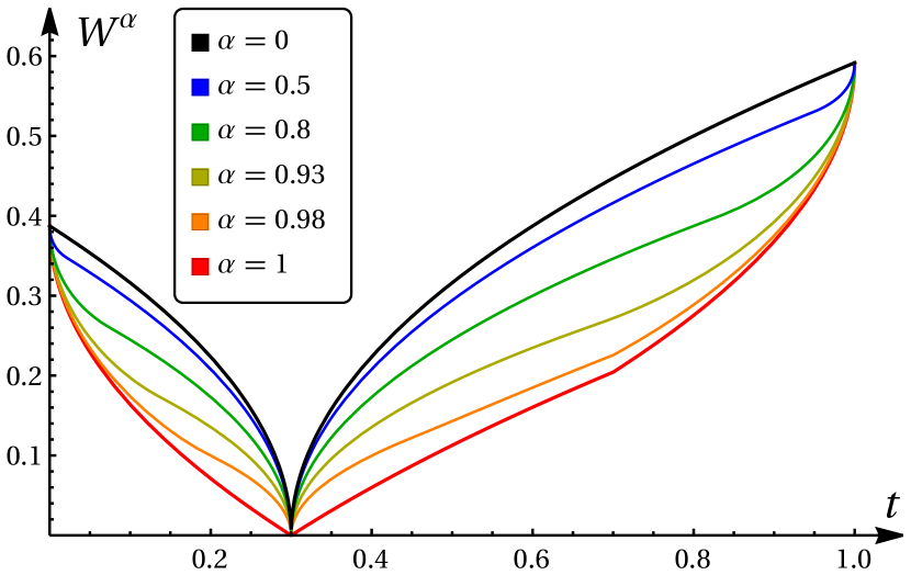
Figure 4: An illustration of quantum-to-classical transition of the transport problem. The plot shows how the distance $W^{\alpha}(\operatorname{diag}(0.3,0.7),\operatorname{diag}(t,1-t))$ increases with the coherence parameter decreasing from $\alpha=1$ (quantum) to $\alpha=0$ (classical) case.

Appendix I Cost matrices for larger dimensions

Let us discuss here the transport distance between two mixed states of size $N>2$. In the case of a qutrit ($N=3$) the quantum cost matrix (Eq. (6) in the main body of the article) for the configuration of the equilateral triangle, $E_{12}=E_{13}=E_{23}=1$, takes the form

$$C^{Q}\vcentcolon=\frac{1}{2}\left[\begin{array}[]{lllllllll}0&0&0&0&0&0&0&0&0\\ 0&1&0&\!\!\!\!-1&0&0&0&0&0\\ 0&0&1&0&0&0&\!\!\!\!-1&0&0\\ 0&\!\!\!\!-1&0&1&0&0&0&0&0\\ 0&0&0&0&0&0&0&0&0\\ 0&0&0&0&0&1&0&\!\!\!\!-1&0\\ 0&0&\!\!\!\!-1&0&0&0&1&0&0\\ 0&0&0&0&0&\!\!\!\!-1&0&1&0\\ 0&0&0&0&0&0&0&0&0\end{array}\right].$$ (39)

Observe that the above matrix can be taken to block-diagonal form by a suitable permutation. Note that the corresponding classical cost function, $C^{cl}={\rm diag}(C^{Q})$, in two-index notation, reads $C^{cl}_{ij,ij}=1$ if $i\neq j$ and $C^{cl}_{ii,ii}=0$.

Numerical results suggest that, as in the qubit case, the root transport cost for qutrits, $W=\sqrt{T^{Q}}$, satisfies the triangle inequality, while the latter fails for $W_{1}=T^{Q}$. We have also checked that this extends to ququarts ($N=4$), with $C^{Q}=\tfrac{1}{2}\big{(}\mathbbm{1}_{16}-S\big{)}$.

It is also natural to consider a set of three ordered points on a line equipped with the Euclidean distance, $E_{12}=E_{23}=~{}1,E_{13}=2$. The corresponding classical cost matrix is defined as

$$(C^{cl}_{E})_{ij,ij}=|i-j|,\quad i,j=1,\dots,N.$$ (40)

The quantization (Eq. (15) in the main body of the article) of such $C^{cl}_{E}$ reads

$$C^{Q}_{E}\vcentcolon=\frac{1}{2}\left[\begin{array}[]{lllllllll}0&0&0&0&0&0&0&0&0\\ 0&1&0&\!\!\!\!-1&0&0&0&0&0\\ 0&0&2&0&0&0&\!\!\!\!-2&0&0\\ 0&\!\!\!\!-1&0&1&0&0&0&0&0\\ 0&0&0&0&0&0&0&0&0\\ 0&0&0&0&0&1&0&\!\!\!\!-1&0\\ 0&0&\!\!\!\!-2&0&0&0&2&0&0\\ 0&0&0&0&0&\!\!\!\!-1&0&1&0\\ 0&0&0&0&0&0&0&0&0\end{array}\right],$$ (41)

so that $C^{Q}_{E}\geq 0$ and diag$(C^{Q}_{E})=C^{cl}_{E}$.

Under such a choice the quantum Kantorovich–Wasserstein distance is no longer unitarily invariant, as the distance from $|1\rangle$ to $|3\rangle$ is larger than from $|1\rangle$ to $|2\rangle$, but such a property is desirable to get the correct classical limit ZS98 ; ZS01 .

To generalize this expression for an arbitrary dimension $N$ we can use the notion of maximally entangled states $|\psi^{-}_{ij}\rangle$ which act on a two dimensional subspace. The corresponding cost matrix for the transport problem is then given by a weighted combination of projections onto antisymmetric subspaces,

$$C^{Q}_{E}=\sum_{j>i=1}^{N}|i-j|\;|\psi^{-}_{ij}\rangle\langle\psi^{-}_{ij}|.$$ (42)

Observe that, in contrast to the simplex case, such $C^{Q}_{E}$ is no longer a projection, and the quantum transport cost $T_{E,p}^{Q}$ does depend on the choice of parameter $p\geq 1$. We have checked numerically that while $\sqrt{T_{E,1}^{Q}}$ seems to enjoy the triangle inequality, this is not the case for either $\sqrt{T_{E,2}^{Q}}$ or $T_{E,1}^{Q}$.

Based on numerical results we are tempted to conjecture that for any classical geometry $E$ on the $N$-point space and any three quantum states $\rho^{A},\rho^{B},\rho^{C}\in\Omega_{N}$ one has

$$\sqrt{T^{Q}_{E,1}(\rho^{A},\rho^{B})}+\sqrt{T^{Q}_{E,1}(\rho^{A},\rho^{B})}\geq\sqrt{T^{Q}_{E,1}(\rho^{A},\rho^{B})}.$$

Moreover, the two quantities $\sqrt{T_{E,2}^{Q}}$ and $T_{E,1}^{Q}$ give distances between basis states $|i\rangle$ and $|j\rangle$ consistent with the classical distance matrix $E_{ij}$.

Appendix J Coupling matrices in the Fano form

When analyzing density matrices of order $N=2$ it is convenient to use the set of three Pauli matrices, which generate the group $\mathrm{SU}(2)$. These traceless matrices, often denoted as $\sigma_{1},\sigma_{2}$ and $\sigma_{3}$, together with the identity matrix, $\sigma_{0}:={\mathbbm{1}}_{2}$, form an orthogonal basis in the Hilbert-Schmidt space of Hermitian matrices of dimension $2$. Hence, any $2\times 2$ Hermitian matrix $\rho$ can be expanded in this basis,

$$\rho=\frac{1}{2}\sigma_{0}+\frac{1}{2}\sum_{i=1}^{3}\tau_{i}\sigma_{i},$$ (43)

where the expansion coefficients are given by $\tau_{i}={\rm Tr}\rho\sigma_{i}$. Since the state $\rho$ is Hermitian these three numbers are real. The vector $\tau$ of length three is called the Bloch vector of $\rho$, and if its length satisfies condition $\|\tau\|^{2}\leq 1$ , then the matrix $\rho$ is positive semidefinite and represents a legitimate quantum state BZ17 .

In the general case of a state $\rho$ of dimension $N$ the generalized Bloch vector $\tau$ consists of $N^{2}-1$ components, and the set of three Pauli matrices is replaced by the collection of $N^{2}-1$ traceless Hermitian matrices $\Lambda_{i}$ which satisfy the orthogonality relation Tr$\Lambda_{i}\Lambda_{j}=2\delta_{ij}$ and generate the group $\mathrm{SU}(N)$. This yields the expansion

$$\rho=\frac{1}{N}{\mathbbm{1}}_{N}+\frac{1}{N}\sum_{i=1}^{N^{2}-1}\tau_{i}\Lambda_{i}.$$ (44)

Usually the order of the generators is not relevant, but for our purposes it is convenient to select first $N-1$ generators $\Lambda_{i}$ as diagonal ones. Then any classical probability vector $p$ of size $N$ from the probability simplex, $\Delta_{N}$, can be expressed in its Bloch form, which can be considered as a special case of formula (44) above,

$$p=\frac{1}{N}\;{\rm diag}({\mathbbm{1}}_{N})+\frac{1}{N}\sum_{i=1}^{N-1}\tau_{i}\;{\rm diag}(\Lambda_{i}).$$ (45)

Here the first $N-1$ generators $\{\Lambda_{i}\}_{i=1}^{N-1}$ are represented by diagonal traceless matrices of dimension $N$. The first term simply represents the flat vector, $p_{*}=(1,\dots,1)/N$, while the second one describes the translation vector $\tilde{\tau}$ inside the simplex, which consists of the first $N-1$ components of the Bloch vector $\tau$ of length $N^{2}-1$.

Now consider an arbitrary state $\rho^{AB}$ of a bipartite $N\times N$ system. In full analogy with the Bloch representation (44), one can expand it in the product basis, $\Lambda_{i}\otimes\Lambda_{j}$ with $i,j=0,\dots N^{2}-1$. In this way one arrives at the Fano representation Fa83 of a bipartite state,

$$\rho^{AB}=\frac{1}{N^{2}}\sum_{i,j=0}^{N^{2}-1}M_{ij}\Lambda_{i}\otimes\Lambda_{j},$$ (46)

where $M_{ij}=\frac{N^{2}}{4}{\rm Tr}\rho^{AB}\Lambda_{i}\otimes\Lambda_{j}$. Since we have selected $\Lambda_{0}={\mathbbm{1}}_{N^{2}}$, the matrix of coefficients $M_{ij}$ takes the form

$$M=\left[\begin{array}[]{ll}1&\ a^{T}\\ b&\ R\\ \end{array}\right],\$$ (47)

where $R$ is a real correlation matrix of order $N^{2}-1$, while the vectors $a$ and $b$ of length $N^{2}-1$ determine the Bloch vectors of both partial traces, $a=\tau_{A}$, $\rho^{A}={\rm Tr}_{B}\rho^{AB}$, and $b=\tau_{B}$, $\rho^{B}={\rm Tr}_{A}\rho^{AB}$, respectively. This representation is useful to determine the maximal fidelity of a given two-qubit state with respect to maximally entangled states BH300 , and to formulate separability criteria for bipartite systems Vi07 . The matrix (47) allows us to represent any bipartite state by specifying both local states and their correlations, $\rho^{AB}=\rho^{AB}(\tau_{A},\tau_{B},R)$.

In the special case of a diagonal state $\rho^{AB}$, any bipartite probability vector $p^{AB}\in\Delta_{N^{2}}$ can be written as $p^{AB}=p^{AB}(\tilde{\tau_{A}},\tilde{\tau_{B}},\tilde{R})$. Here $\tilde{\tau_{A}}$ and $\tilde{\tau_{B}}$ denote vectors formed from the first $N-1$ components of the Bloch vectors $\tau_{A}$ and $\tau_{B}$, respectively, which, according to (45), determine both marginal probability vectors, $p^{A}$ and $p^{B}$. The classical correlation matrix $\tilde{R}$ of order $N-1$ forms the upper left corner of the full correlation matrix $R$ of order $N^{2}-1$ in (47).

In the one-qubit case, $N=2$, the real matrix $R$ of order three can be taken to diagonal form via real singular value decomposition, $R\to R^{\prime}=O_{1}RO_{2}$ where $O_{1},O_{2}\in SO(3)$, so that $R^{\prime}$ is diagonal and its entries $v_{1},v_{2},v_{3}$, are real and can be negative. If both partial traces of $\rho^{AB}$ are maximally mixed, $\rho^{A}=\rho^{B}={\mathbbm{1}}/2$, so that both Bloch vectors vanish, $\tau_{A}=\tau_{B}=0$, the correlation matrix $R$ represents a positive density matrix $\rho^{AB}$ if the vector $\vec{v}$ of three real singular values of $R$ belongs to the regular tetrahedron inscribed in the cube $[-1,1]^{3}$ – see BH300 . In the general case of larger dimensions and non-zero Bloch vectors the conditions for the correlation matrix $R$ to assure positivity of the state $\rho^{AB}$ are not easy to provide in an analytical form, so one has to rely on numerical techniques.

The Fano form (46) of a bipartite state is useful to describe the set $\Gamma^{Q}$ of couplings in the quantum transport problem. As the vectors $a$ and $b$ of length $N^{2}-1$ appearing in the matrix (47) represent both partial traces, we need to fix them by the Bloch vectors $\tau_{A}$ and $\tau_{B}$ of the analyzed states $\rho^{A}$ and $\rho^{B}$. Thus, the minimization in Eq. (8) in the main body of the article is taken over the set of correlation matrices $R$ for which the density matrix $\rho^{AB}$ determined by matrix (47) is positive semidefinite,

$$\Gamma^{Q}(\rho^{A},\rho^{B})=\{\rho^{AB}(\tau_{A},\tau_{B},R):\rho^{AB}\geq 0\}.$$ (48)

We recall here some properties of the set of couplings and the extremal points of this set analyzed in Ru04 ; Pa05 ; LPW14 :

For any two states $\rho^{A}$ and $\rho^{B}$ of dimension $N$ the set $\Gamma^{q}(\rho^{A},\rho^{B})$ of admissible couplings:

a) includes the product state, $\rho^{A}\otimes\rho^{B}\in\Gamma^{q}(\rho^{A},\rho^{B})$.

b) forms a convex subset of the set $\Omega_{N^{2}}$ of all bipartite states. If $\rho^{AB}(\tau_{A},\tau_{B},R_{1})\in\Gamma^{q}$ and $\rho^{AB}(\tau_{A},\tau_{B},R_{2})\in\Gamma^{q}$, then any convex combination thereof forms a density matrix, $x\rho^{AB}(\tau_{A},\tau_{B},R_{1})+(1-x)\rho^{AB}(\tau_{A},\tau_{B},R_{2})\in\Gamma^{q}$ for $x\in[0,1]$, as any convex combination of two positive matrices is positive.

c) contains a state of rank one (a projector onto a pure state) iff both arguments have the same spectrum: $|\psi\rangle\langle\psi|\in\Gamma^{q}(\rho^{A},\rho^{B})\Leftrightarrow{\rm Eig}(\rho^{A})={\rm Eig}(\rho^{B})$. This statement holds as for any pure state in a bipartite system both reduced density matrices (obtained by partial traces) have the same spectrum, so that they are unitarily similar, $\rho^{B}=U\rho^{A}U^{\dagger}$. The spectrum of reduced states determines the Schmidt vector BZ17 of the bipartite pure state $|\psi\rangle$.

As a minimum of a linear function over a convex set is attained at its boundary, due to item c) above the extreme of the quantum transport problem in the case of two states with different spectra can be achieved for a bipartite state $\rho^{AB}$ of rank $2,3,\dots,N^{2}-1$. The question concerning the relation between the spectrum of a bipartite state $\rho^{AB}$ and the spectra of its partial traces, $\rho^{A}$ and $\rho^{B}$, is known as the quantum marginal problem. In the simplest case of two states of size $N=2$ this problem was solved by Bravyi Br04 , while a general theory providing the solution for larger dimensions was developed by Klyachko Kl04 .

Appendix K Transport problem and quantum operations

A completely positive, trace preserving linear map $\Phi$ acting on the set $\Omega_{N}$ of quantum states is called a quantum operation or quantum channel. Its action on a given state $\rho$ can be conveniently written in Kraus form, $\rho^{\prime}=\Phi(\rho)=\sum_{j=1}^{r}K_{j}\rho K_{j}^{\dagger}$. The number $r$ of Kraus operators $K_{j}$ is arbitrary, but to ensure the trace preserving condition they must satisfy the identity resolution $\sum_{j=1}^{r}K_{j}^{\dagger}K_{j}={\mathbbm{1}}$ – see BZ17 .

Making use of the Bloch representation (44), let us represent the initial state $\rho$ by the Bloch vector $\tau$ and its image $\rho^{\prime}$ by the transformed vector $\tau^{\prime}$. In this way one can rewrite any quantum operation as a linear action on Bloch vectors,

$$\tau^{\prime}=Q\tau+\kappa,$$ (49)

where the real distortion matrix $Q$ has dimension $N^{2}-1$, and $\kappa$ is a translation vector of the same length, which vanishes for unital maps. Hence, the superoperator $\Phi$ can be represented by an asymmetric real matrix of order $N^{2}$,

$$\Phi\;=\;\left[\begin{array}[]{ll}1&0\\ {\vec{\kappa}}&{Q}\end{array}\right].$$ (50)

The above form, also called the Liouville representation of a map KR01 ; KSRJO14 , is convenient for spectral analysis: the spectrum of the superoperator $\Phi$ consists of the leading Frobenius–Perron eigenvalue, $\lambda_{1}=1$, and the $N^{2}-1$ eigenvalues of the real matrix $Q$, which can be complex.

Apparent similarity between the form (50) of an arbitrary operation $\Phi$ and the matrix (47) is not accidential, as it is a consequence of representing the Jamiołkowski–Choi state $J=(\Phi\otimes{\mathbbm{1}})|\phi_{+}\rangle\langle\phi_{+}|$ belonging to the extended space of size $N\times N$ in Fano form. Here $|\phi_{+}\rangle=\frac{1}{\sqrt{N}}\sum_{j=1}^{N}|j,j\rangle$ denotes the maximally entangled Bell state BZ17 . Note that the vector $a$ in (47) vanishes due to the trace-preserving condition.

Returning now to the transport problem and the set $\Gamma^{Q}(\rho^{A},\rho^{B})$ of admissible couplings (48), we see that in general the Fano form (47) does not describe quantum operations which send the initial state $\rho^{A}$ to the final state $\rho^{B}$. In fact, for an arbitrary initial Bloch vector $a=\tau_{A}\neq 0$, the corresponding transformation $\Phi$ is not trace preserving. However, in the particular case of an initial state which is maximally mixed, $\rho^{A}={\mathbbm{1}}/N$, the corresponding Bloch vector vanishes, $\tau_{A}=0$, and the final Bloch vector, $\tau_{B}=Q\tau_{A}+b$, indeed represents the final state $\rho^{B}$ with the Bloch vector $\tau_{B}=b$. In such a case optimization over the set of all admissible couplings $\Gamma^{Q}$ can be considered as optimization over the set of quantum operations, parametrized by the distortion matrix $Q$, which transforms the initial maximally mixed state, $\rho^{A}={\mathbbm{1}}/N$, into the final state $\rho^{B}$, as expected in the transport problem.

The dual condition, $b=0$, corresponds to unital maps which preserve identity, so bistochastic operations, $a=b=0$, are represented by Choi matrices with both states maximally mixed. Extremal points of the set of these tracial states were analyzed by Ohno Oh10 .

Note that the cost matrix $C^{Q}$ of order 4, defined in Eq. (7) in the main body of the article, forms the Choi matrix corresponding to the rotation $\Phi_{y}$ with respect to the $y$ axis,

$$C^{Q}=(\Phi_{y}\otimes\mathbbm{1}){|\phi_{+}\rangle}{\langle\phi_{+}|}=(\sigma_{2}\otimes\mathbbm{1}){|\phi_{+}\rangle}{\langle\phi_{+}|}(\sigma_{2}\otimes\mathbbm{1}),$$ (51)

equivalent to the projector onto the singlet state ${|\psi_{-}\rangle}$.

The problem of quantum optimal transport was recently related to the question of determining the distinguished quantum channel that, for a given input state, produces a prescribed output state DPT19 ; Du20a .

References

(1) I. Bengtsson and K. Życzkowski,
Geometry of Quantum States. 2 ed., Cambridge 2017.
(2) G. Monge,
Mémoire sur la théorie des déblais et des remblais,
Histoire de l’Académie Royale des Sciences de Paris, 1781.
(3) S. Rachev and L. Rüschendorf,
Mass Transportation Problems, Vol. I and II,
Springer, New York, 1998.
(4) T. Salvemini,
Sul calcolo degli indici di concordanza tra due caratteri quantitativi,
Atti della VI Riunione Soc. Ital. di Statistica, Roma (1943).
(5) L. V. Kantorovich.
On the translocation of masses.
Dokl. Akad. Nauk. USSR37, 199 (1942).
(6) L. V. Kantorovich, On a problem of Monge,
Uspekhi Mat. Nauk.3, 225 (1948).
(7) L.N. Wasserstein,
Markov processes over denumerable products of spaces describing large systems of automata, Probl. Inform. Transmission5, 47 (1969).
(8) C. Villani,
Optimal Transport. Old and New,
Springer-Verlag, Berlin, Heidelberg, 2009.
(9) A. M. Vershik,
Long history of the Monge-Kantorovich transportation problem,
Math. Intelligencer35, 1 (2013).
(10)
P. Biane and D. Voiculescu,
A free probability analogue of the Wasserstein metric on the trace-state space,
Geom. Funct. Anal.11, 1125 (2001).
(11) M. Eckstein and T. Miller,
Causality for Nonlocal Phenomena,
Ann. Henri Poincaré18, 3049 (2017).
(12) M. Eckstein and T. Miller,
Causal evolution of wave packets,
Phys. Rev. A95, 032106 (2017).
(13) M. Eckstein, P. Horodecki, T. Miller and R. Horodecki,
Operational causality in spacetime,
Phys. Rev. A101, 042128 (2020).
(14) K. Życzkowski and W. Słomczyński,
Monge distance between quantum states,
J.Phys.A 31, 9095-9104, (1998).
(15) K. Życzkowski and W. Słomczyński,
The Monge metric on the sphere and geometry of quantum states,
J. Phys.A 34, 6689 (2001).
(16) K. Życzkowski, H. Wiedemann, and W. Słomczyński,
How to generalize Lapunov exponent for quantum mechanics,
Vistas Astronomy37, 153 (1993).
(17) Z. Wang, Y. Wang and B. Wu,
Genuine quantum chaos and physical distance between quantum states,
Phys. Rev.E 103, 042209 (2021).
(18) J. Agredo and F. Fagnola,
On quantum versions of the classical Wasserstein distance,
Stochastics89, 910 (2017).
(19) F. Golse and T. Paul,
Wave packets and the quadratic Monge-Kantorovich distance in quantum mechanics,
Comptes Rendus Math.356, 177 (2018).
(20) Y. Chen, T. T. Georgiou and A. Tannenbaum,
Wasserstein geometry of quantum states
and optimal transport of matrix-valued measures,
in Emerging Applications of Control and Systems Theory,
p. 139 Springer, (2018).
(21)
F. Golse, C. Mouhot, and T. Paul, On the Mean Field and Classical Limits of Quantum Mechanics, Commun. Math. Phys. 343, 165–205 (2016).
(22)
Y. Chen, T. T Georgiou, L. Ning, and A. Tannenbaum,
Matricial Wasserstein- distance,
IEEE Control Systems Lett.1, 14 (2017).
(23) R. Bhatia, S. Gaubert and T. Jain,
Matrix versions of the Hellinger distance,
preprint arXiv:1901.01378
(24) S. Friedland, J. Ge and L. Zhi, Quantum Strassen’s theorem,
arXiv:1905.06865,
Infinite Dimensional Analysis, Quantum Probability and Related Topics,
23, 2050020 (2020).
(25) S. Friedland,
Tensor optimal transport, distance between sets of measures and tensor scaling, preprint arXiv:2005.00945.
(26) Y. Chen, W. Gangbo, T. T. Georgiou, and A. Tannenbaum,
On the matrix Monge-Kantorovich problem,
Eur. J. Appl. Math.31, 574 (2020).
(27) R. Duvenhage,
Quadratic Wasserstein metrics for von Neumann algebras via transport plans,
preprint arXiv:2012.03564
(28) N. Yu, L. Zhou, S. Ying and M. Ying,
Quantum earth mover’s distance, no-go quantum
Kantorovich-Rubinstein theorem, and quantum marginal problem,
preprint arXiv:1803.02673v2.
(29) M.H. Reira, A transport approach to distances in quantum systems, Bachelor’s Thesis Universitat Autònoma de Barcelona (2018).
(30)
K. Ikeda, Foundation of quantum optimal transport and applications,
Quantum Inform. Process.19, 25 (2020).
(31) G. De Palma, M. Marvian, D. Trevisan and S. Lloyd, The Quantum Wasserstein Distance of Order 1, IEEE Transactions on Information Theory (2021), doi: 10.1109/TIT.2021.3076442.
(32) G. De Palma and D. Trevisan,
Quantum optimal transport with quantum channels, Annales Henri Poincaré (2021),
doi: 10.1007/s00023-021-01042-3.
(33) E. A. Carlen and J. Maas,
Non-commutative calculus, optimal transport and
functional inequalities in dissipative quantum systems,
J. Stat. Phys.178, 319 (2020).
(34) N. Datta and C. Rouzé,
Relating relative entropy, optimal transport and
Fisher information: A quantum HWI inequality.
Ann. H. Poincaré21, 2115 (2020).
(35) E. Caglioti, F. Golse, and T. Paul,
Quantum optimal transport is cheaper,
J. Stat. Phys., 181, 149 (2020).
(36) S. L. Braunstein and C. M. Caves,
Statistical distance and the geometry of quantum states,
Phys. Rev. Lett.72, 3439 (1994).
(37) D. Šafránek,
Discontinuities of the quantum Fisher information and the Bures metric,
Phys. Rev.A 95, 052320 (2017).
(38) J. Liu, H. Yuan, X.-M. Lu, and X. Wang,
Quantum Fisher information matrix and multiparameter estimation,
J. Phys.A53, 023001 (2020).
(39) J. Biamonte, P. Wittek, N. Pancotti, P. Rebentrost, N. Wiebe, N., and S. Lloyd, Quantum machine learning, Nature549, 195 (2017).
(40) S. Lloyd, and C. Weedbrook, Quantum Generative Adversarial Learning, Phys. Rev. Lett.121, 040502 (2018).
(41) S. Chakrabarti, Y. Huang, T. Li, S. Feizi, and X. Wu,
Quantum Wasserstein Generative Adversarial Networks,
in Advances in Neural Information Processing Systems, ID:3674 (2019).
(42) B.T. Kiani, G. De Palma, M. Marvian, Z.-W. Liu, and S. Lloyd,
Quantum Earth Mover’s Distance: A New Approach to Learning Quantum Data,
preprint arXiv:2101.03037 (2021).
(43) A. Uhlmann,
The ‘transition probability’ in the state space of a *-algebra,
Rep. Math. Phys.9, 273 (1976).
(44) R. Jozsa,
Fidelity for mixed quantum states,
J. Mod. Opt. 41, 2315–23 (1994).
(45) K.R. Parthasarathy,
Extreme points of the convex set of joint probability
distributions with fixed marginals,
Proc. Indian Acad. Sci. (Math. Sci.)117, 505 (2007).
(47) A. Winter, Tight uniform continuity bounds for quantum entropies: conditional entropy, relative entropy distance and energy constraints, Commun. Math. Phys.347, 291–313 (2016).
(48) K. Korzekwa, S. Czachórski, Z. Puchała
and K. Życzkowski, Coherifying quantum channels,
N. J. Phys.20, 043028 (2018).
(49) A. Gilchrist, N. K. Langford, M. A. Nielsen,
Distance measures to compare real and ideal quantum processes,
Phys. Rev.A 71, 062310 (2005).
(50) A. Uhlmann, Geometric phases and related structures,
Rep. Math. Phys.36, 461 (1995).
(51) J. A. Miszczak, Z. Puchala, P. Horodecki, A. Uhlmann, K. Życzkowski, Sub-and super-fidelity as
bounds for quantum fidelity, Quantum Inf. Comp.9, 0103-0130 (2009).
(52) J. Briët and P. Harremoës,
Properties of classical and quantum Jensen-Shannon divergence,
Phys. Rev.A 79, 052311 (2009).
(53) D. Virosztek,
The metric property of the quantum Jensen–Shannon divergence,
Advances in Mathematics380, 107595 (2021).
(54) A. Uhlmann, Spheres and hemispheres as quantum state spaces, J. Geom. Phys.18, 76–92 (1996).
(55) T. Baumgratz, M. Cramer, and M. B. Plenio,
Quantifying coherence,
Phys. Rev. Lett.113, 140401 (2014).
(56) W. H. Zurek, Decoherence, einselection, and the quantum origins of the classical, Rev. Mod. Phys.75, 715 (2003).
(57) P.-L. Dallaire-Demers, and N. Killoran, Quantum generative adversarial networks, Phys. Rev. A98, 0122324 (2018).
(58) M. Arjovsky, S. Chintala, L. Bottou, Wasserstein Generative Adversarial Networks, Proceedings of Machine Learning Research70, 214 (2017).
(59) A. N. Pechen, and D.J. Tannor, Are there traps in quantum control
landscapes?, Phys. Rev. Lett, 106, 120402 (2011).
(60) J. R. McClean, S. Boixo, V. N. Smelyanskiy, R. Babbush, and H. Neven, Barren plateaus in quantum neural network training landscapes, Nat. Comm.9, 4812 (2018).
(61) S. Wang, E. Fontana, M. Cerezo, K. Sharma, A. Sone, L. Cincio, and P.J. Coles, Noise-induced barren plateaus in variational quantum algorithms, preprint arXiv:2007.14384 (2020).
(62) M. Cerezo, A. Sone, T. Volkoff, L. Cincio, and P. J. Coles, Cost-function-dependent barren plateaus in shallow quantum neural networks, Nat. Comm.12, 1791 (2021).
(63) S. Cole, M. Eckstein, S. Friedland and K. Życzkowski, Quantum Optimal Transport, preprint arXiv:2105.06922 (2021).
(64) R.F. Werner, Quantum states with Einstein–Podolsky–Rosen correlations admitting a hidden-variable mode, Phys. Rev. A40, 4277 (1989).
(65) C.A. Fuchs, and J. van de Graaf, Cryptographic Distinguishability Measures for Quantum Mechanical States, IEEE Trans. Inf. Theory45, 1216 (1999).
(67) J. Maas, Gradient flows of the entropy for finite Markov chains, J. Funct. Anal.261, 2250–2292 (2011).
(68) U. Fano, Pairs of two-level systems,
Rev. Mod. Phys.55, 855 (1983).
(69) P. Badzia̧g, M. Horodecki, P. Horodecki, and R. Horodecki.
Local environment can enhance fidelity of quantum teleportation,
Phys. Rev.A62 012311, (2000).
(70) J. I. de Vincente,
Separability criteria based on the Bloch representation of density matrices,
Quantum Inf. Comput.7, 624 (2007).
(71) O. Rudolph,
On extremal quantum states of composite systems with fixed marginals
J. Math. Phys.45, 4035 (2004).
(72) K. R. Parthasarathy,
Extremal quantum states in coupled systems,
Ann. Inst. H. Poincaré, Probab. Stat.41, 257 (2005).
(73) C.-K. Li, Y.-T. Poon and X. Wang,
Ranks and eigenvalues of states with prescribed reduced states,
Electronic J. Lin. Algebra27, 935 (2014).
(74) S. Bravyi,
Requirments for compatibility between local and multipartite quantum states,
Quantum Inf. Comp.4, 12 (2004).
(75) A. Klyachko,
Quantum marginal problem and representations of the symmetric group,
preprint quant-ph/0409113 (2004).
(76) C. King and M. B. Ruskai,
Minimal entropy of states emerging from noisy quantum channels,
IEEE Trans. Inf. Theory47, 192 (2001).
(77) S. Kimmel, M. P. da Silva, C. A. Ryan, B. R. Johnson,
and T. Ohki,
Robust extraction of tomographic information via randomized benchmarking,
Phys. Rev.X 4, 011050 (2014).
(78) H. Ohno,
Maximal rank of extremal marginal tracial states,
J. Math. Phys.51, 092101 (2010).