New Determinations of the UV Luminosity Functions from $z\sim 9$ to $z\sim 2$ show a remarkable consistency with halo growth and a constant star formation efficiency

Abstract

Here we provide the most comprehensive determinations of the rest-frame $UV$ LF available to date with HST at $z\sim 2$, 3, 4, 5, 6, 7, 8, and 9. Essentially all of the non-cluster extragalactic legacy fields are utilized, including the Hubble Ultra Deep Field (HUDF), the Hubble Frontier Field parallel fields, and all five CANDELS fields, for a total survey area of 1136 arcmin². Our determinations include galaxies at $z\sim 2$-3 leveraging the deep HDUV, UVUDF, and ERS WFC3/UVIS observations available over a $\sim$150 arcmin² area in the GOODS North and GOODS South regions. All together, our collective samples include $>$24,000 sources, $>$$2.3\times$ larger than previous selections with HST. 5766, 6332, 7240, 3449, 1066, 601, 246, and 33 sources are identified at $z\sim 2$, 3, 4, 5, 6, 7, 8, and 9, respectively. Combining our results with an earlier $z\sim 10$ LF determination by Oesch et al. (2018a), we quantify the evolution of the $UV$ LF. Our results indicate that there is (1) a smooth flattening of the faint-end slope $\alpha$ from $\alpha\sim-2.4$ at $z\sim 10$ to $-1.5$ at $z\sim 2$, (2) minimal evolution in the characteristic luminosity $M^{*}$ at $z\geq 2.5$, and (3) a monotonic increase in the normalization $\log_{10}\phi^{*}$ from $z\sim 10$ to $z\sim 2$, which can be well described by a simple second-order polynomial, consistent with an “accelerated” evolution scenario. We find that each of these trends (from $z\sim 10$ to $z\sim 2.5$ at least) can be readily explained on the basis of the evolution of the halo mass function and a simple constant star formation efficiency model.

1. Introduction

Quantifying the build-up of galaxies in the early universe remains one of a principal area of interest in extragalactic astronomy involves (e.g., Madau & Dickinson 2014; Davidzon et al. 2017). Studies of galaxy build-up have become increasingly mature, with ever more detailed efforts to measure the star formation rates and stellar masses of galaxies (e.g., Salmon et al. 2015; Leja et al. 2019; Stefanon et al. 2021, in prep). Determinations of the volume density in the context of star formation rate and stellar mass measurements allow for connections to the underlying dark matter halos (e.g., Behroozi et al. 2013; Harikane et al. 2016, 2018; Stefanon et al. 2017a).

One prominent, long-standing gauge of galaxy build-up is the luminosity function of galaxies in the rest-frame $UV$, which represents the volume density of galaxies as a function of the $UV$ luminosity. As the time-averaged star formation rate of galaxies is proportional to the unobscured luminosities of galaxies in the rest-frame $UV$, the $UV$ luminosity function provides us with a measure of how quickly galaxies grow with cosmic time.

There is already significant work on the $UV$ LF across a wide range in redshifts, from local studies to studies in the early universe. Broadly, the normalization $\phi^{*}$ and faint-end slope $\alpha$ of the $UV$ LF have been found to increase and to flatten, respectively, with cosmic time (Bouwens et al. 2015, 2017; Finkelstein et al. 2015; Bowler et al. 2015; Parsa et al. 2016; Ishigaki et al. 2018), while the characteristic luminosity remains fixed with cosmic time (Bouwens et al. 2015, 2017; Finkelstein et al. 2015; Bowler et al. 2015; Parsa et al. 2016) or becomes fainter (Arnouts et al. 2005). Motivated by many theoretical models, Bouwens et al. (2015) showed that the evolution of the faint-end slope from $z\sim 8$ to $z\sim 4$ could be naturally explained by a similar steepening of the halo mass function over the relevant range (see also Mason et al. 2015; Tacchella et al. 2013, 2018).

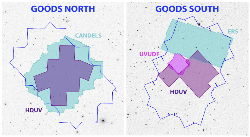
Figure 1.— The layout of the search fields we utilize with WFC3/UVIS $UV_{275}U_{336}$ $\sim$0.25-0.4$\mu$m data to identify $z\sim 2$-3 galaxies. These include the $\sim$93 arcmin² HDUV fields (Oesch et al. 2018b), the $\sim$7 arcmin² UVUDF field (Teplitz et al. 2013), and the $\sim$50 arcmin² ERS (Windhorst et al. 2011) data set. The cyan footprint shown over the GOODS-North shows the WFC3/UVIS imaging data available from the CANDELS program in the F275W (Grogin et al. 2011) and has an exposure time equivalent to $\sim$6 orbits (Oesch et al. 2018b). All together we leverage a $\sim$150 arcmin² search area to identify $>$11,000 $z\sim 2$-3 galaxies over GOODS South and GOODS North.

Given the increasing clarity in the general evolutionary trends in the $UV$ LF with redshift, galaxy evolution studies are entering an era where precision measurements become increasingly key. To date, there has been no systematic, self-consistent determination of the evolution of the rest-frame $UV$ LF from $z\sim 9$ to $z\sim 2$.

The availability of deep wide-area WFC3/UVIS observations from the HDUV program (Oesch et al. 2018b) as well as the previously existing WFC3/UVIS observations from the WFC3/IR Early Release Science (ERS) and UVUDF programs (Windhorst et al. 2011; Teplitz et al. 2013) allow us to extend the Bouwens et al. (2015) study of the $UV$ LF down to $z\sim 2$, while adding valuable statistics and leverage at the bright and faint ends.

In addition, through inclusion of observations from the Hubble Frontier Fields program (Lotz et al. 2017), we can further refine our earlier determinations of the $UV$ LF at $z\sim 4$-10 published in Bouwens et al. (2015). Importantly, the HFF parallel data probe $\sim$1 mag fainter than the CANDELS data set, providing us with probes of the volume density of galaxies at magnitude levels intermediate between the CANDELS and XDF/HUDF regimes.

In the present determinations of the $UV$ LF, we expressly focus on blank field search results for $z\sim 2$-9 galaxies. We exclude search results behind lensing clusters to ensure that the present $UV$ LF determinations are only impacted by systematic errors specific to blank field studies (Bouwens et al. 2017a, Bouwens et al. 2017b; Atek et al. 2018). In a follow-up paper (Bouwens et al. 2021, in prep), we will provide separate determinations of the $UV$ LF using observations over the Hubble Frontier Fields clusters, and then we will compare the LF results from the lensing fields with the blank fields and test for consistency.

We now present a plan for this paper. §2 provides a brief description of the data sets used in this study, our procedure for deriving the photometry, and the selection criteria utilized in this study. In §3, we summarize our procedure for deriving LF results, while also presenting our new UV LF results. In §4, we discuss the new trends we find and compare our new LF results with previous results in the literature. Finally, §5 summarizes our results.

For convenience, we quote results in terms of the approximate characteristic luminosity $L_{z=3}^{*}$ derived at $z\sim 3$ by Steidel et al. (1999), Reddy & Steidel (2009), and many other studies. We refer to the HST F225W, F275W, F336W, F435W, F606W, F600LP, F775W, F814W, F850LP, F098M, F105W, F125W, F140W, and F160W bands as $UV_{225}$, $UV_{275}$, $U_{336}$, $B_{435}$, $V_{606}$, $V_{600}$, $i_{775}$, $I_{814}$, $z_{850}$, $Y_{098}$, $Y_{105}$, $J_{125}$, $JH_{140}$, and $H_{160}$, respectively, for simplicity. The standard concordance cosmology $\Omega_{0}=0.3$, $\Omega_{\Lambda}=0.7$, and $H_{0}=70\,\textrm{km/s/Mpc}$ is assumed for consistency with previous LF studies. All magnitudes are in the AB system (Oke & Gunn 1983).

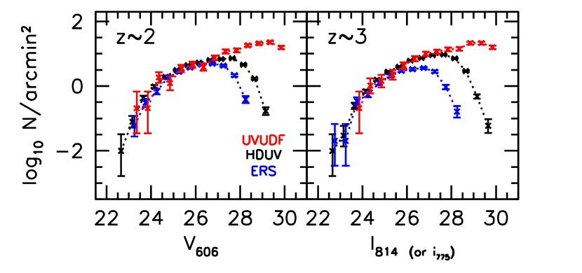
Figure 2.— Surface densities of the candidate $z\sim 2$ and $z\sim 3$ galaxies for the three search fields considered in this analysis, i.e., ERS (blue points), HDUV (black points), and the UVUDF (red points). Surface densities are presented as a function of the $V_{606}$ and $I_{814}$ band magnitudes that provide the best measure of the rest-frame $UV$ flux of galaxies at 1600$\AA$ for our $z\sim 2$ and $z\sim 3$ selections, respectively. For the UVUDF $z\sim 3$ results, the $i_{775}$ band magnitudes are presented here instead (due to the significantly greater depth of the $i_{775}$-band data). A slight horizontal offset of the points relative to each other has been applied for clarity. The onset of incompleteness in our different samples is clearly seen in the observed decrease in surface density of sources near the magnitude limit. We do not make use of the faintest sources in each search field, i.e., $V_{606}/i_{775}/I_{814}$ magnitudes fainter than 26.5, 28.0, and 29.0 for the ERS, HDUV, and UVUDF fields, respectively, given the large uncertainties in the completeness (and contamination) corrections.

2. Data Sets and Catalogues

2.1. HDUV + ERS

The primary data for our $z=2$-3 LF results are the sensitive near-UV observations obtained over a $\sim$94 arcmin² area within the GOODS-South and GOODS-North fields using the HDUV program (Oesch et al. 2018b). For a description of the characteristics and reduction of those data, we refer the interested reader to Oesch et al. (2018b). Optical and near-IR observations over this field were obtained by making use of the v1.0 Hubble Legacy Field (HLF: Illingworth et al. 2016; Whitaker et al. 2019; G.D. Illingworth et al. 2021, in prep) reductions. The HLF reductions constitute a comprehensive reduction of all the archival optical/ACS + near-IR/WFC3/IR observations over the GOODS-South and GOODS-North fields.

For our $z=2$-3 selections and LF results, we also make use of the WFC3/UVIS $UV_{225}UV_{275}U_{336}$ observations that were part of the WFC3 ERS program over the GOODS South field. These data cover $\sim$50 arcmin². The ERS observations, together with the HDUV observations, cover an area of 143 arcmin² in total. First selections of $z\sim 2$-3 galaxies from those data sets and rest-frame $UV$ LF results were obtained by Hathi et al. (2010) and Oesch et al. (2010). As in the case of the HDUV data, we make use of the reduction of optical and near-IR observations over the ERS area from the HLF program.

Table 1Total number of sources in the $z\sim 2$, $z\sim 3$, $z\sim 4$, $z\sim 5$, $z\sim 6$, $z\sim 7$, $z\sim 8$, $z\sim 9$, and $z\sim 10$ samples from this paper and Oesch et al. 2018a

	Area	$z\sim 2$	$z\sim 3$	$z\sim 4$	$z\sim 5$	$z\sim 6$	$z\sim 7$	$z\sim 8$	$z\sim 9$	$z\sim 10$
Field	(arcmin2)	#	#	#	#	#	#	#	#
From Bouwens et al. 2015 and 2016 (see also Oesch et al. 2013, 2014)
HUDF/XDF	4.7	—	—	357	153	97	57	29	—	—
HUDF09-1	4.7	—	—	—	91	38	22	18	—	0
HUDF09-2	4.7	—	—	147	77	32	23	15	—	0
CANDELS-GS-DEEP	64.5	—	—	1590	471	198	77	26	2	1
CANDELS-GS-WIDE	34.2	—	—	451	117	43	5	3	0	0
ERS	40.5	—	—	815	205	61	46	5	2	0
CANDELS-GN-DEEP	68.3	—	—	1628	634	188	134	51	1	2
CANDELS-GN-WIDE	65.4	—	—	871	282	69	39	18	0	1
CANDELS-UDS	151.2	—	—	—	270	33	18	6	1	0
CANDELS-COSMOS	151.9	—	—	—	320	48	15	9	1	0
CANDELS-EGS	150.7	—	—	—	381	50	43	9	2	1
BORG/HIPPIES	218.3	—	—	—	—	—	—	23	—	—
HDUV + ERS + UVUDF (This Work [§2.6])
HDUV-GOODS-S (+ UVUDF)	43.5	2127	2454	—	—	—	—	—	—	—
ERS	49.2	1252	1055	—	—	—	—	—	—	—
HDUV-GOODS-N	57.6	2387	2823	—	—	—	—	—	—	—
From CANDELS COSMOS/UDS/EGS Fields (Bouwens et al. 2019 and This Work (§2.8])
CANDELS-UDS	45.3	—	—	—	—	—	—	—	1	0
CANDELS-COSMOS	48.7	—	—	—	—	—	—	—	0	0
CANDELS-EGS	53.4	—	—	—	—	—	—	—	4	0
Hubble Frontier Fields Parallels (This Work [§2.7,2.8] + Oesch et al. 2018a)
Abell 2744-Par	4.9	—	—	226	67	20	11	4	3	0
MACS0416-Par	4.9	—	—	266	71	25	19	4	3	0
MACS0717-Par	4.9	—	—	214	55	41	21	10	0	0
MACS1149-Par	4.9	—	—	234	76	36	31	6	1	0
Abell S1063-Par	4.9	—	—	231	79	40	20	7	2	0
Abell 370-Par	4.9	—	—	210	100	47	20	3	4	2
HFF Total	29.4	—	—	1381	448	209	122	34	13	2
Hubble Ultra Deep Field + Parallels (This Work [§2.8] + Oesch et al. 2018a)
HUDF/XDF	4.9	—	—	—	—	—	—	—	4	1
HUDF09-1	4.9	—	—	—	—	—	—	—	0	0
HUDF09-2	4.9	—	—	—	—	—	—	—	2	0
Total	1135.9	5766	6332	7240	3449	1066	601	246	33	8

Figure 1 shows the layout of the WFC3/UVIS observations from the HDUV and ERS fields over the GOODS-South and GOODS-North fields.

2.2. UVUDF/XDF

We also made use of near-UV, optical, and near-IR observations over the HUDF from the UVUDF program (Teplitz et al. 2013), optical ACS HUDF program (Beckwith et al. 2016), HUDF09/HUDF12 programs (Bouwens et al. 2011; Ellis et al. 2013), and any other HST observations that have been taken over the HUDF/XDF. Illingworth et al. (2013) combined all existing optical and near-IR observations over the HUDF (including many archival observations) into an especially deep reduction called the eXtreme Deep field (XDF). The XDF optical reductions include all ACS and WFC3/IR data on the HUDF through 2013 and are $\sim$0.1-0.2 mag deeper than the Beckwith et al. (2006) reductions of the optical ACS data.

We make use of the v2.0 reductions of the epoch 3 WFC3/UVIS data over the HUDF acquired in post-flash mode (to cope with CTE degradation: see Rafelski et al. 2015). Observations for epoch 3 of the UVUDF program were divided equally across the F225W, F275W, and F336W bands, with 15 orbits of time allocated to each band. The $5\sigma$ depths we measure for the epoch-3 UVUDF data in $0.4^{\prime\prime}$-diameter apertures are 27.1, 27.2, and 27.8 mag, respectively. No use was made of the first 45 orbits of data from the UVUDF program, given the impact of CTE degration on those data which were acquired without post-flash (see Teplitz et al. 2013).

2.3. Parallel Fields to the Hubble Ultra Deep Field

Another valuable data set we use for our $z\sim 9$ search are the two flanking fields to the HUDF, i.e., HUDF09-1 and HUDF09-2 (Oesch et al. 2007; Bouwens et al. 2011) where sensitive observations have been obtained with both ACS and WFC3/IR. These observations could be obtained efficiently due to simultaneous observing programs over the HUDF and due to the parallel observing capabilities of HST. A total of 8, 12, and 13 orbits in the $Y_{105}$, $J_{125}$, and $H_{160}$ bands, respectively, were obtained over HUDF09-1 parallel field, while 11, 18, and 19 orbits in the $Y_{105}$, $J_{125}$, $H_{160}$ bands, respectively, were obtained over HUDF09-2 parallel field. Very deep ($>$100 orbits) optical data in the $V_{606}i_{775}I_{814}z_{850}$ bands also exist over these two fields from the HUDF05, HUDF09, HUDF12, and other programs (Oesch et al. 2007; Bouwens et al. 2011; Ellis et al. 2013).

2.4. Hubble Frontier Fields Parallels

In addition to the data already utilized in Bouwens et al. (2015) and Bouwens et al. (2016) for blank-field LF results at $z=4$, 5, 6, 7, 8, and 9, we also add the sensitive optical and near-IR observations obtained over six deep parallel fields from the HFF program (Coe et al. 2015; Lotz et al. 2017). These deep parallel fields supplement the deep optical and near-IR observations obtained by the HFF program over the centers of six different clusters (Abell 2744, MACS0416, MACS0717, MACS1149, Abell 370, and Abell S1063) and are separated from the cluster centers by $\sim$8 arcmin. 70 orbits of optical ACS observations (18, 10, and 42 in the F435W, F606W, and F814W bands, respectively) and 70 orbits of WFC3/IR observations (24, 12, 10, and 24 in the F105W, F125W, F140W, and F160W bands, respectively) were invested in observations of each parallel field. We made use of the v1.0 reductions of these observations made publicly available by the HFF team (Koekemoer et al. 2014).

In addition to making use of the available HST observations, we also made use of the $\sim$50-80 hours of Spitzer/IRAC observations over the parallel fields to the HFF clusters to allow for the selection of galaxies to $z\sim 9$. The available observations were drizzled together to construct sensitive mosaics of each cluster at $\sim$3-5 microns (as performed by Labbé et al. 2015 and Stefanon et al. 2020).

Table 2A complete list of the sources included in the $z\sim 2$, $z\sim 3$, $z\sim 4$, $z\sim 5$, $z\sim 6$, $z\sim 7$, $z\sim 8$, $z\sim 9$, and $z\sim 10$ samples from the present selection and that of Oesch et al. 2018a

ID	R.A.	Dec	$m_{AB}$	Sample	Data Set	$z_{phot}$
XDFB-2384848214	03:32:38.49	$-$27:48:21.4	27.77	4	1	3.49
XDFB-2384248186	03:32:38.42	$-$27:48:18.7	29.18	4	1	3.82
XDFB-2376648168	03:32:37.66	$-$27:48:16.9	28.61	4	1	4.01
XDFB-2385948162	03:32:38.60	$-$27:48:16.2	28.04	4	1	4.16
XDFB-2382548139	03:32:38.26	$-$27:48:13.9	28.18	4	1	4.37
XDFB-2394448134	03:32:39.45	$-$27:48:13.4	26.40	4	1	3.58
XDFB-2381448127	03:32:38.14	$-$27:48:12.7	28.58	4	1	3.68
XDFB-2390248129	03:32:39.03	$-$27:48:13.0	27.99	4	1	3.91
XDFB-2379348121	03:32:37.93	$-$27:48:12.1	27.45	4	1	4.11
XDFB-2378848108	03:32:37.88	$-$27:48:10.9	30.13	4	1	3.72

2.5. Source Detection and Photometry

Our procedures for pursuing source detection and photometry are very similar to most of our previous work (e.g., Bouwens et al. 2011, 2015). We use the SExtractor software (Bertin & Arnouts 1996) to handle source detection and photometry. We run the SExtractor software in dual-image mode, with the detection image taken to equal the square root of $\chi^{2}$ image (Szalay et al. 1999: similar to a coadded image) constructed from the $V_{606}i_{775}I_{814}z_{850}$ images for our $z\sim 2$-3 selections, constructed from the $Y_{105}J_{125}JH_{140}H_{160}$ images for our $z\sim 4$-7 selections, $J_{125}JH_{140}H_{160}$ images for our $z\sim 8$ selections, and $JH_{140}$ and $H_{160}$ images for our $z\sim 9$ selections. Color measurements are made in small scalable apertures (Kron [1980] factor of 1.2), after PSF-matching the observations to the $z_{850}$ band (if the color measurement only includes the optical bands) or the $H_{160}$ band (if the color measurement includes a near-infrared band).

Measurements of the total magnitude are made by correcting the smaller-scalable aperture flux measurements to account for the excess flux measured in the larger-scalable apertures relative to the smaller-scalable apertures and also for the light on the wings on the PSF (typically a $\sim$0.15-0.25 mag correction) using the tabulated values of the encircled energy distributions (Dressel et al. 2012).

For $z\sim 9$ selections, only the HST $JH_{140}$ and $H_{160}$ probe the spectral slope of galaxies redward of the Lyman-break providing us with very limited leverage to distinguish bona-fide star-forming galaxies at $z\sim 9$ from lower-redshift interlopers. Therefore, for our $z$$\sim$9 selections, we also derive fluxes for individual sources at $\sim$3.6$\mu$m and 4.5$\mu$m using the mophongo software (Labbé et al. 2006, 2010a, 2010b, 2013, 2015). Deriving fluxes for sources in the $3.6\mu$m and $4.5\mu$m bands is challenging due to the broad PSF of the Spitzer/IRAC data, which causes light from neighboring sources to blend together on the images. To overcome these issues, mophongo uses the high spatial resolution HST data to create template images of each source in the lower spatial resolution Spitzer/IRAC data and then the fluxes of the source and its neighbors is varied to obtain the best fit. The model profiles of the neighboring sources is then subtracted from the image, and then the flux of the source is measured in $1.8^{\prime\prime}$-diameter apertures. These fluxes are then extrapolated to total based on the model profile of the source convolved with the PSF.

In selecting candidate $z=2$-9 galaxies, we required the candidate galaxies in our $z\sim 2$-3, $z\sim 4$-7, $z\sim 8$, and $z\sim 9$ samples to show a S/N of 5.5, 5.5, 6, and 6.5, respectively, in the $\chi^{2}$ images used to detect sources. Sources which correspond to diffraction spikes, are the clear result of an elevated background around a bright source (e.g., for a bright elliptical galaxy), or correspond to other artifacts in the data are removed by visual inspection.

We clean the sample by removing all bright ($H_{160,AB}<27$) sources with SExtractor stellarity parameters in excess of 0.9, i.e., star-like. SExtractor stellarity parameters of 0 and 1 correspond to extended and point sources, respectively. We also removed all sources with whose SExtractor stellarity parameter is in excess of 0.6 and whose HST photometry is much better fit with an SED of a low-mass star ($\Delta\chi^{2}>2$) from the SpeX library (Burgasser et al. 2004) than with a linear combination of galaxy templates from EAZY (Brammer et al. 2008).

2.6. Selection of $z=2$-3 Galaxies

As in our own previous searches for $z\sim 2$-9 galaxies (e.g., Oesch et al. 2010; Oesch et al. 2013; Bouwens et al. 2015), we required sources to satisfy Lyman-break-like criteria for inclusion in our samples. In fact, spectroscopic follow-up work has demonstrated that Lyman-break-like color-color criteria provide a very efficient way of identifying $z\sim 3$-8 Lyman-break galaxies (e.g., Steidel et al. 1999; Steidel et al. 2003; Vanzella et al. 2009; Stark et al. 2010; Ono et al. 2012; Finkelstein et al. 2013; Oesch et al. 2015; Zitrin et al. 2015; Hashimoto et al. 2018).

In our selection of galaxies for our $z\sim 2$ and $z\sim 3$ samples from the HDUV and ERS data, we first apply the following criteria to our source catalogs:

$$(UV_{275}-B_{435}>1)\wedge$$

$$((V_{606}-z_{850}<0.5)\vee$$

$$((UV_{275}-B_{435}>2(V_{606}-z_{850}))\wedge$$

$$(V_{606}-z_{850}<1.0)))$$

or

$$(UV_{336}-V_{606}>1)\wedge$$

$$((V_{606}-z_{850}<0.5)\vee$$

$$((UV_{336}-V_{606}>2(V_{606}-z_{850}))\wedge$$

$$(V_{606}-z_{850}<1.0)))\wedge(\textrm{SN}(UV_{275})<2)$$

where $\wedge$, $\vee$, and SN represents the logical AND operation, the logical OR operation, and signal to noise computed in small scalable apertures, respectively. The fluxes of sources not detected are set to the $1\sigma$ upper limits on the flux in the undetected band.

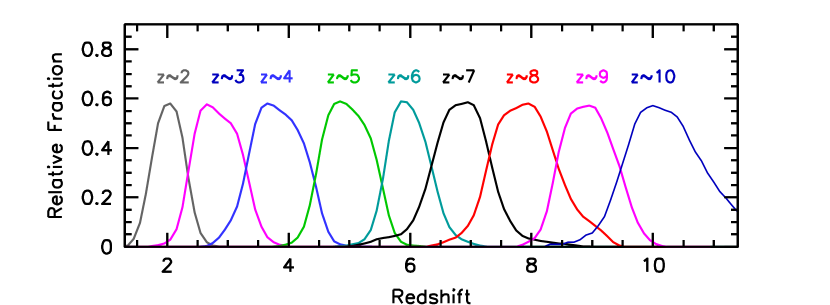
Figure 3.— Shown is the approximate redshift distribution expected for sources in our selections of $z\sim 2$, $z\sim 3$, $z\sim 4$, $z\sim 5$, $z\sim 6$, $z\sim 7$, $z\sim 8$, and $z\sim 9$ galaxies with the grey, magenta, blue, green, cyan, black, red, and magenta lines, respectively. The expected redshift distributions shown here are based on our HDUV and HUDF/XDF selection volume simulation results at $z\sim 2$-3 and $z\sim 4$-9, respectively. The dark blue line shows the expected redshift distribution for the $z\sim 10$ selection from the companion study of Oesch et al. (2018a). The precise redshift distribution exhibits a modest dependence on the available HST passbands for a data set, as illustrated e.g. in Figure 4 of Bouwens et al. (2015).

We then make use of the photometric redshift software EAZY (Brammer et al. 2008) to determine the redshift likelihood distribution for each source. Consideration was made of the photometry we derived in the WFC3/UVIS (UV₂₇₅, $U_{336}$), ACS ($B_{435}$, $V_{606}$, $i_{775}$, $I_{814}$, $z_{850}$), and WFC3/IR ($Y_{098}$, $Y_{105}$, $J_{125}$, $JH_{140}$, and $H_{160}$) bands. The SED templates we used were the EAZY_v1.0 set supplemented by SED templates from the Galaxy Evolutionary Synthesis Models (GALEV: Kotulla et al. 2009). Nebular continuum and emission lines were added to the later templates using the Anders & Fritze-v. Alvensleben (2003) prescription, a $0.2Z_{\odot}$ metallicity, and a rest-frame EW for H$\alpha$ of 1300Å. To allow for possible systematics in our photometry and differences between the observed and model SEDs, we assume an additional 7% uncertainty in our flux measurements when deriving photometric redshifts with EAZY.

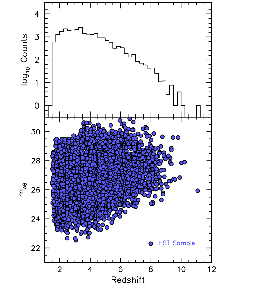
Figure 4.— (upper) Histogram of the # of sources vs. redshift for the HST selections considered here. (lower) Redshift vs. apparent magnitudes (blue filled circles) for all sources in the present HST samples (and those of Oesch et al. 2018a). The source at $z\sim 11.1$ and with an $H_{160,AB}$ magnitude of 25.9 mag is GN-z11 (Bouwens et al. 2010; Oesch et al. 2014, 2016).

For selection, we additionally required that $>$65% of the integrated probability in the photometric redshift likelihood distribution lie at $>$1.2 and for the best-fit $\chi^{2}$ be less than 25 (equivalent to $\chi_{reduced}^{2}\lesssim 2.5$) to include sources where we can obtain a reasonable SED fit to the photometry. Sources where the best-fit photometric redshift lie in the range $z=1.5$-2.5 and $z=2.5$-3.5 are placed in our $z\sim 2$ and $z\sim 3$ samples, respectively.

2.7. Selection of $z=4$-8 Galaxies

As in previous work (Bouwens et al. 2015), we select $z=4$-9 galaxies from the HFF parallel fields using Lyman-break color criteria. Sources in our $z\sim 4$ samples are selected following these criteria:

$$(B_{435}-V_{606}>1.0)\wedge(I_{814}-J_{125}<1.0)\wedge$$

$$(B_{435}-V_{606}>1.0+1.77(I_{814}-J_{125})\wedge$$

$$\textrm{[not in}\,z\sim 5\,\,\textrm{samples]}$$

Our $z\sim 5$ samples are selected using the following color criteria:

$$(V_{606}-I_{814}>1.2)\wedge$$

$$(V_{606}-I_{814}>1.32+1.2(Y_{105}-H_{160}))\wedge$$

$$(Y_{105}-H_{160}<0.9)\wedge(\textrm{SN}(B)<2)\wedge$$

$$\textrm{[not in}\,z\sim 6-7\,\,\textrm{samples]}$$

For our $z\sim 6$ and $z\sim 7$ samples, we select sources using the following color criteria:

$$(I_{814}-Y_{105}>0.6)\wedge(Y_{105}-H_{160}<0.45)\wedge$$

$$(I_{814}-Y_{105}>0.6(Y_{105}-H_{160}))\wedge$$

$$(Y_{105}-H_{160}<0.52+0.75(J_{125}-H_{160})\wedge$$

$$\textrm{SN}(B_{435}<2)\wedge$$

$$((\chi_{opt}^{2}(B_{435},V_{606})<2)\vee(V_{606}-Y_{105}>2.5))\wedge$$

$$\textrm{[not in}\,z\sim 8\,\,\textrm{samples]}$$

where $\chi_{opt}^{2}$ is calculated as follows $\chi_{opt}^{2}=\Sigma_{i}\textrm{SGN}(f_{i})(f_{i}/\sigma_{i})^{2}$ where $f_{i}$ is the flux in band $i$ in a consistent aperture, $\sigma_{i}$ is the uncertainty in this flux, and SGN($f_{i}$) is equal to 1 if $f_{i}>0$ and $-1$ if $f_{i}<0$ (see Bouwens et al. 2011).

For our $z\sim 8$ selection, we apply the following criteria:

$$(Y_{105}-J_{125}>0.45)\wedge$$

$$(Y_{105}-J_{125}>0.525+0.75(J_{125}-H_{160})\wedge$$

$$(J_{125}-H_{160}<0.5)\wedge(\chi_{opt,0.35^{\prime\prime}}^{2}<4)\wedge$$

$$(\chi_{opt,Kron}^{2}<4)\wedge(\chi_{opt,0.2^{\prime\prime}}^{2}<4)\wedge$$

$$\textrm{[not in}\,z\sim 9\,\,\textrm{samples]}$$

Sources in our $z\sim 8$ sample must have a $\chi^{2}$ statistic less than 4 (i.e., $<$2$\sigma$ detection) combining the $B_{435}$, $V_{606}$, and $I_{814}$-band flux measurements in both small scalable apertures and fixed 0.35^′′-diameter apertures.

We divide the $z\sim 6$-7 selection into $z\sim 6$ and $z\sim 7$ samples using the photometric redshift we compute for individual sources using the EAZY photometric redshift software (Brammer et al. 2008). Sources with a photometric redshift $z<6.3$ are assigned to our $z\sim 6$ sample provided that the fractional likelihood of the source lying at $z<4.3$ is $<$35%, whereas sources with a photometric redshift $z>6.3$ are assigned to our $z\sim 7$ selection. Sources in our $z\sim 7$ sample must have a $\chi^{2}$ statistic less than 4 (i.e., $<$2$\sigma$ detection) combining the $B_{435}$ and $V_{606}$ flux measurements in small scalable apertures and fixed 0.35^′′-diameter apertures.

2.8. Selection of $z\sim 9$ Galaxies

In selecting candidate $z\sim 9$ galaxies from the HFF parallel fields and the XDF, both of which have deep $JH_{140}$ observations, we make use fo the following color criteria to identify candidate $z\gtrsim 9$ galaxies:

$$((Y_{105}-H_{160})+2(J_{125}-JH_{140})>1.5)\wedge$$

$$((Y_{105}-H_{160})+2(J_{125}-JH_{140})>$$

$$~{}~{}~{}~{}~{}~{}~{}1.5+1.4(JH_{140}-H_{160}))\wedge$$

$$((Y_{105}-H_{160})+(Y_{105}-JH_{140})>2)\wedge$$

$$(JH_{140}-H_{160}<0.5)\wedge(\chi_{opt,0.35^{\prime\prime}}^{2}<4)\wedge$$

$$(\chi_{opt,Kron}^{2}<4)\wedge(\chi_{opt,0.2^{\prime\prime}}^{2}<4)$$

where $\chi_{opt,0.35^{\prime\prime}}^{2}$, $\chi_{opt,Kron}^{2}$, and $\chi_{opt,0.2^{\prime\prime}}^{2}$, respectively, represent the “$\chi^{2}$” statistic computed from the optical fluxes in 0.35^′′-diameter apertures, small-scalable Kron apertures, and small 0.2^′′-diameter apertures (before PSF-matching the optical data to the lower resolution near-IR data).

For the two deep parallel fields to the HUDF, HUDF09-1 and HUDF09-2, deep $JH_{140}$-band data are not available, and so we utilize the following color criteria:

$$((Y_{105}-H_{160})+2(J_{125}-H_{160})>1.5)\wedge$$

$$(J_{125}-H_{160}<1.2)\wedge(\chi_{opt,0.35^{\prime\prime}}^{2}<4)\wedge$$

$$(\chi_{opt,Kron}^{2}<4)\wedge(\chi_{opt,0.2^{\prime\prime}}^{2}<4)$$

In cases of a non-detection, the measured fluxes are set to their $1\sigma$ upper limits for the purposes of deriving measured colors to apply the above criteria.

Our $z\sim 9$ selection criteria are modified from those presented in Oesch et al. (2013). This is in an attempt to contrast the “average” flux information in the $Y_{105}$ and $J_{125}$ bands and the “average” flux information in the $JH_{140}$ and $H_{160}$ bands to measure the size of the apparent break in the spectrum of candidate $z\sim 9$ galaxies. In computing the $\chi^{2}$ statistic for sources in our $z\sim 9$ selections, we included the fluxes in all optical ACS bands blueward of $Y_{105}$.

To maximize the robustness of the sources in our selection, we also made use of the Spitzer/IRAC observations of the $z\sim 9$ candidates to examine the color of the sources redward of the nominal Lyman break. We considered both our own photometry on each candidate and that from Shipley et al. (2018) for those sources falling within the HFF parallel fields. Given the challenges of obtaining Spitzer/IRAC flux measurements in the presence of source crowding, we only excluded sources if they showed at least a $3\sigma$ detection both from our own photometry and that from Shipley et al. (2018) and if the source showed a $H_{160}-[3.6]$ color redder than 0.7 mag.

Finally, sources are required to have a best-fit photometric redshift calculated with EAZY between $z=8.4$ and $z=9.5$ and to have $>$70% of the redshift likelihood distribution above $z\sim 7$. We used the same SED template set to compute this redshift likelihood distribution as we used in §2.6.

Our $z\sim 9$ selection also includes sources identified over the five CANDELS fields and ERS field, a 874 arcmin² area. While we have already provided an extensive description of this selection in Bouwens et al. (2019), some additional $Y_{098}$ and $JH_{140}$ imaging has become available on $z\sim 9$ candidates from that selection thanks to observations from HST programs 15103 (PI: de Barros) and 15862 (PI: Finkelstein). $Y_{098}$ and $Y_{105}$-band observations from those program further confirm the nature of COS910-1, EGS910-9, and EGS910-10, with estimated $P(z>8)$ probabilities of 0.97, 0.75, and 1.0, respectively, and strengthen the case that EGS910-15 is at $z>8$, with $P(z>8)$ being 0.56.

Our previous $z\sim 4$-10 LF study (Bouwens et al. 2015) made no use of a separate $z\sim 9$ selection, and therefore many $z\sim 9$ galaxies might have been included in their $z\sim 7$ and $z\sim 8$ samples (which included a tail extending up to $z\sim 9$). We therefore inspected the $z\sim 7$ and $z\sim 8$ samples from Bouwens et al. (2015) to search for overlap with our new $z\sim 9$ samples and eliminated any sources in common (10 candidates). Additionally, we recomputed the selection volumes from Bouwens et al. (2015) to explicitly exclude sources that would also satisfy the present $z\sim 9$ selection criteria.

2.9. Derived Samples of $z\sim 2$-9 Galaxies

Applying our selection criteria to the WFC3/UVIS + optical ACS + WFC3/IR observations over the GOODS South and GOODS North fields, we identify a total of 5766 $z\sim 2$ galaxies and 6332 $z\sim 3$ galaxies. The surface density of sources in our $z\sim 2$ selections as a function of the apparent magnitude in the $V_{606}$ band is shown in Figure 2, while the surface densities of our $z\sim 3$ HDUV, UVUDF, and ERS samples are presented as a function of the $I_{814}$, $i_{775}$, and $i_{775}$ band magnitudes, respectively. These bands probe close to 1600Å in the rest frame.

For comparison, Hathi et al. (2010) identified 66 $z\sim 1.7$ $UV_{225}$ dropouts, 151 $z\sim 2.1$ $UV_{275}$ dropouts, and 256 $z\sim 2.7$ $U_{336}$ dropouts over the $\sim$50 arcmin² WFC3/IR ERS field. Meanwhile, Oesch et al. (2010) find 60 $UV_{225}$, 99 $UV_{275}$, and 403 $U_{336}$ dropouts over the same ERS field. Combining the individual subsamples, Hathi et al. (2010) and Oesch et al. (2010) find 473 $z\sim 2$-3 and 562 $z\sim 2$-3 galaxies over the ERS field. While we find a much larger number of sources over the ERS, i.e., 2307 sources, the $z\sim 2$ and $z\sim 3$ selections of Hathi et al. (2010) and Oesch et al. (2010) cut off approximately $\sim$1.2 mag brightward of our selections due to their use of more restrictive selection criteria. If we similarly cut off our $z\sim 2$ and $z\sim 3$ selections at $\sim$25.5 mag and $\sim$26 mag, we find 876 $z\sim 2$-3 galaxies, which is much more comparable to the numbers in these previous selections.

Using the $\sim$7.3 arcmin² UVUDF data set, Mehta et al. (2017) identify 852 $z\sim 2$-3 galaxies. This is fairly similar (just 20% smaller) than the 1069 $z\sim 2$-3 galaxies we find over the same field. The surface density of $z\sim$2-3 galaxies in the Mehta et al. (2017) samples, i.e., 120 galaxies arcmin^-2, is also comparable, but 29% larger, than the 93 galaxy arcmin^-2 surface density we find over the HDUV fields. It is because of the combination of depth and area of the current UVUDF+UVUDF data sets, i.e., $\sim$1-mag greater depth than ERS and 21 $\times$ larger area than UVUDF+HDUV data sets relative to previousERS and UVUDF data sets alone that the present $z\sim 2$-3 samples are $>$10$\times$ larger than the previous $z\sim 2$-3 samples of Hathi et al. (2010), Oesch et al. (2010), and Mehta et al. (2017).

For our $z\sim 4$, $z\sim 5$, $z\sim 6$, $z\sim 7$, $z\sim 8$, and $z\sim 9$ selections over the HFF parallel fields, a total of 1381, 448, 209, 122, 34, and 13 galaxies are identified. Adding to these new sources to those sources found in the Bouwens et al. (2015) samples from the HUDF/XDF, the HUDF parallel fields, BoRG, and the five CANDELS fields, our total samples of $z\sim 4$, $z\sim 5$, $z\sim 6$, $z\sim 7$, $z\sim 8$, $z\sim 9$ are 7240, 3449, 1066, 601, 246, and 33. These sources are in addition to the 9 sources in the $z\sim 10$-11 samples of Oesch et al. (2018a), for which this analysis was done in coordination. Table 1 summarizes the number of sources in each of the samples we consider. The total size of our HST samples at $z=2$-11 is 24741, 12643 of which are in the redshift range $z\sim 4$-11. Table 2 presents the complete catalog of these sources, with coordinates, apparent magnitudes, and photometric redshift estimates.

The expected redshift distributions for our $z\sim 2$, $z\sim 3$, $z\sim 4$, $z\sim 5$, $z\sim 6$, $z\sim 7$, $z\sim 8$, and $z\sim 9$ selections are shown in Figure 3, along with the redshift distribution for the $z\sim 10$ selection from Oesch et al. (2018).

The top panel of Figure 4 shows the total number of the sources per unit $\Delta z\sim 0.25$, while the lower panel shows the full distribution of magnitudes and redshifts that sources in our samples occupy.

Table 3Magnification Factors Adopted for Each of the HFF Parallel Fields

Field	Typical Magnification Factor $\mu$
Abell 2744-Par	1.16
MACS0416-Par	1.05
MACS0717-Par	1.16
MACS1149-Par	1.04
Abell S1063-Par	1.05
Abell 370-Par	1.10

3. Luminosity Function Results

The purpose of the present section is to summarize our procedures for deriving the $UV$ LFs at $z\sim 2$, 3, 4, 5, 6, 7, 8, and 9. The present determinations leverage a variety of new data sets to improve on the results obtained in Oesch et al. (2010), Bouwens et al. (2015), and Bouwens et al. (2016).

Given that the present analysis aims to improve on earlier LF analyses from Oesch et al. (2010), Bouwens et al. (2015), and Bouwens et al. (2016), our new determinations still incorporate constraints from earlier data sets, such as the HUDF, the two HUDF parallel fields, the WFC3/IR ERS field, the five CANDELS fields, and 220 arcmin² in search area from BoRG+HIPPIES utilized in Bouwens et al. (2015) and Bouwens et al. (2016). We also include $z\sim 2$ and $z\sim 3$ samples from the UVUDF and WFC3/UVIS ERS fields.

Our procedure for deriving the selection volumes is identical to that described in Appendix D of Bouwens et al. (2015) and involves creating artificial sources with a variety of apparent magnitudes and redshifts using our artificial redshifting code (Bouwens et al. 1998; Bouwens et al. 2003), adding those sources to the observations, and then selecting those sources in the same way as we do with the real observations. In creating artificial sources for our $z\sim 2$-3 selection volume simulations, we used the pixel-by-pixel morphologies of similar-luminosity galaxies from our $z\sim 2$ HUDF samples, scaling them in size as $(1+z)^{-1.2}$ and using the same $UV$ color distribution as Bouwens et al. (2009) and Bouwens et al. (2014). Selection volumes for our UVUDF selections are created in a similar way, but computing photometric redshifts for the sources detected in the simulations and applying our selection criteria to determine if a simulated source is selected or not. Since these simulations use similar-luminosity $z\sim 2$ galaxies from the HUDF to simulate galaxies at $z\sim 3$ or in shallower fields (like the HDUV or ERS fields), they implicitly account for the size-luminosity relation. Selection volumes for our $z\sim 4$-9 samples follow the same procedure, but start with a random ensemble of $z\sim 4$ galaxies from the HUDF/XDF data as selected by Bouwens et al. (2015).

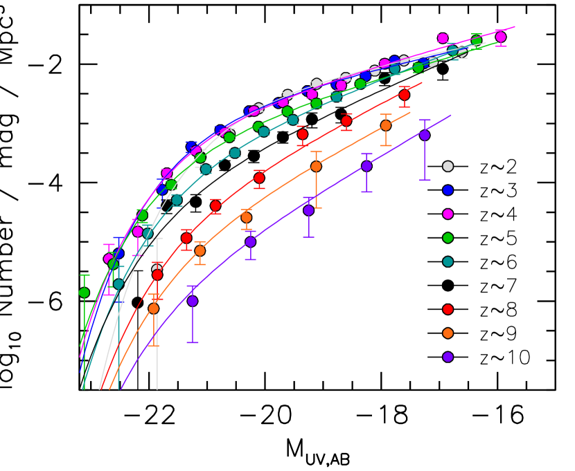
Figure 5.— The stepwise LF constraints (solid circles)) we derive on the $UV$ LFs at $z\sim 2$, $z\sim 3$, $z\sim 4$, $z\sim 5$, $z\sim 6$, $z\sim 7$, $z\sim 8$, and $z\sim 9$ based on our comprehensive blank-field searches with HST (shown in grey, blue, magenta, green, cyan, black, red, orange, and dark purple, respectively). The recent stepwise LF constraints at $z\sim 10$ from Oesch et al. (2018a) are shown with the dark purple circles. The best-fit Schechter LFs are shown with the grey, blue, magenta, green, cyan, black, red, orange, and dark purple lines, respectively.

In deriving LFs from our samples, we need to account for our selections suffering from a low level of contamination from lower redshift sources due to noise in our photometry. Contamination is estimated and included in a very similar way to that done in Bouwens et al. (2015). In the Bouwens et al. (2015) study, contamination rates were estimated by performing degradation experiments on the deepest HST observations. Bona-fide high-redshift sources and low redshift contaminants were first identified in those data. Noise was then added to the observations to emulate the properties of the shallower observations, and sources were selected from these shallower data. The contamination rate was determined by determining which fraction of selected sources in the shallower data were clearly at lower redshift in the deeper data. The typical contamination fractions are estimated to be $\lesssim$5% but reach contamination fractions as high as $\sim$10% in the faintest magnitude bin.

Table 4Stepwise Determination of the rest-frame $UV$ LF at $z\sim 4$, $z\sim 5$, $z\sim 6$, $z\sim 7$, $z\sim 8$, and $z\sim 9$ using the SWML method from the HUDF, HFF parallel fields, and a comprehensive set of blank search fields.

$M_{1600,AB}$	$\phi_{k}$ (Mpc-3 mag-1)	$M_{1600,AB}$	$\phi_{k}$ (Mpc-3 mag-1)	$M_{1600,AB}$	$\phi_{k}$ (Mpc-3 mag-1)
$z\sim 2$ galaxies		$z\sim 5$ galaxies		$z\sim 8$ galaxies
$-$21.86	0.000003$\pm$0.000008	$-$23.11	0.000001$\pm$0.000001	$-$21.85	0.000003$\pm$0.000002
$-$21.11	0.000270$\pm$0.000089	$-$22.61	0.000004$\pm$0.000002	$-$21.35	0.000012$\pm$0.000004
$-$20.61	0.000661$\pm$0.000154	$-$22.11	0.000028$\pm$0.000007	$-$20.85	0.000041$\pm$0.000011
$-$20.11	0.001797$\pm$0.000231	$-$21.61	0.000092$\pm$0.000013	$-$20.10	0.000120$\pm$0.000040
$-$19.61	0.003031$\pm$0.000301	$-$21.11	0.000262$\pm$0.000024	$-$19.35	0.000657$\pm$0.000233
$-$19.11	0.004661$\pm$0.000353	$-$20.61	0.000584$\pm$0.000044	$-$18.60	0.001100$\pm$0.000340
$-$18.61	0.005855$\pm$0.000437	$-$20.11	0.000879$\pm$0.000067	$-$17.60	0.003020$\pm$0.001140
$-$18.11	0.007765$\pm$0.000617	$-$19.61	0.001594$\pm$0.000156
$-$17.61	0.011541$\pm$0.000835	$-$19.11	0.002159$\pm$0.000346	$z\sim 9$ galaxies
$-$17.11	0.010795$\pm$0.002006	$-$18.36	0.004620$\pm$0.000520	$-$21.92	0.000001$\pm$0.000001
$-$16.61	0.015992$\pm$0.003437	$-$17.36	0.008780$\pm$0.001540	$-$21.12	0.000007$\pm$0.000003
		$-$16.36	0.025120$\pm$0.007340	$-$20.32	0.000026$\pm$0.000009
$z\sim 3$ galaxies				$-$19.12	0.000187$\pm$0.000150
$-$22.52	0.000006$\pm$0.000005	$z\sim 6$ galaxies		$-$17.92	0.000923$\pm$0.000501
$-$21.77	0.000076$\pm$0.000038	$-$22.52	0.000002$\pm$0.000002
$-$21.27	0.000402$\pm$0.000078	$-$22.02	0.000014$\pm$0.000005	Oesch et al. (2018a)
$-$20.77	0.000769$\pm$0.000117	$-$21.52	0.000051$\pm$0.000011	$z\sim 10$ galaxies
$-$20.27	0.001607$\pm$0.000157	$-$21.02	0.000169$\pm$0.000024	$-$22.25	$<$0.000002
$-$19.77	0.002205$\pm$0.000189	$-$20.52	0.000317$\pm$0.000041	$-$21.25	0.000001$\pm$0.000001
$-$19.27	0.003521$\pm$0.000239	$-$20.02	0.000724$\pm$0.000087	$-$20.25	0.000010$\pm$0.000005
$-$18.77	0.004557$\pm$0.000297	$-$19.52	0.001147$\pm$0.000157	$-$19.25	0.000034$\pm$0.000022
$-$18.27	0.006258$\pm$0.000437	$-$18.77	0.002820$\pm$0.000440	$-$18.25	0.000190$\pm$0.000120
$-$17.77	0.011417$\pm$0.000656	$-$17.77	0.008360$\pm$0.001660	$-$17.25	0.000630$\pm$0.000520
$-$17.27	0.010281$\pm$0.001368	$-$16.77	0.017100$\pm$0.005260
$z\sim 4$ galaxies		$z\sim 7$ galaxies
$-$22.69	0.000005$\pm$0.000004	$-$22.19	0.000001$\pm$0.000002
$-$22.19	0.000015$\pm$0.000009	$-$21.69	0.000041$\pm$0.000011
$-$21.69	0.000144$\pm$0.000022	$-$21.19	0.000047$\pm$0.000015
$-$21.19	0.000344$\pm$0.000038	$-$20.69	0.000198$\pm$0.000036
$-$20.69	0.000698$\pm$0.000068	$-$20.19	0.000283$\pm$0.000066
$-$20.19	0.001624$\pm$0.000131	$-$19.69	0.000589$\pm$0.000126
$-$19.69	0.002276$\pm$0.000199	$-$19.19	0.001172$\pm$0.000336
$-$19.19	0.003056$\pm$0.000388	$-$18.69	0.001433$\pm$0.000419
$-$18.69	0.004371$\pm$0.000689	$-$17.94	0.005760$\pm$0.001440
$-$17.94	0.010160$\pm$0.000920	$-$16.94	0.008320$\pm$0.002900
$-$16.94	0.027420$\pm$0.003440
$-$15.94	0.028820$\pm$0.008740

Table 5 Determinations of the Schechter Parameters for the rest-frame $UV$ LFs at $z\sim 4$, $z\sim 5$, $z\sim 6$, $z\sim 7$, $z\sim 8$, and $z\sim 9$ from the HUDF, HFF parallels, and a comprehensive set of other blank search fields

Dropout			$\phi^{*}$ $(10^{-3}$
Sample	$<z>$	$M_{UV}^{*}$	Mpc-3)	$\alpha$
$U_{275}$	2.1	$-$20.28$\pm$0.09	4.0${}_{-0.4}^{+0.5}$	$-$1.52$\pm$0.03
$U_{336}$	2.9	$-$20.87$\pm$0.09	2.1${}_{-0.3}^{+0.3}$	$-$1.61$\pm$0.03
$B$	3.8	$-$20.93$\pm$0.08	1.69${}_{-0.20}^{+0.22}$	$-$1.69$\pm$0.03
$V$	4.9	$-$21.10$\pm$0.11	0.79${}_{-0.13}^{+0.16}$	$-$1.74$\pm$0.06
$i$	5.9	$-$20.93$\pm$0.09	0.51${}_{-0.10}^{+0.12}$	$-$1.93$\pm$0.08
$z$	6.8	$-$21.15$\pm$0.13	0.19${}_{-0.06}^{+0.08}$	$-$2.06$\pm$0.11
$Y$	7.9	$-$20.93$\pm$0.28	0.09${}_{-0.05}^{+0.09}$	$-$2.23$\pm$0.20
$J$	8.9	$-$21.15 (fixed)	0.021${}_{-0.009}^{+0.014}$	$-$2.33$\pm$0.19
Oesch et al. (2018a)
$J$	10.2	$-$21.19 (fixed)	0.0042${}_{-0.0022}^{+0.0045}$	$-$2.38$\pm$0.28

In deriving constraints on the $UV$ LF from a comprehensive set of search fields, we rely on the same sample of sources that Bouwens et al. (2015) utilize over all fields, while also including constraints from the new data sets. Combining the new samples with the $z\sim 2$-9 samples from Bouwens et al. (2015) and Bouwens et al. (2016), our new analysis contains contains 5766, 6332, 7240, 3449, 1066, 601, 246, and 33 sources at $z\sim 2$, $z\sim 3$, $z\sim 4$, $z\sim 5$, $z\sim 6$, $z\sim 7$, $z\sim 8$, and $z\sim 9$, respectively.

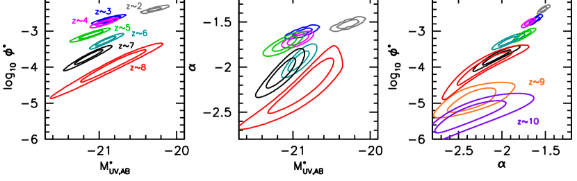
Figure 6.— 68% and 95% confidence intervals on various pairs of parameters in a Schechter representation of the $UV$ LF at $z\sim 2$, $z\sim 3$, $z\sim 4$, $z\sim 5$, $z\sim 6$, $z\sim 7$, $z\sim 8$, $z\sim 9$, and $z\sim 10$. Given our relatively poor constraints on the bright end form of the $z\sim 9$ and $z\sim 10$ LFs and thus $M^{*}$, no confidence intervals are presented in the left and center panels for the LF results at $z\sim 9$ and $z\sim 10$. The $z\sim 10$ constraints are based on the Oesch et al. (2018a) analysis. The normalization $\phi^{*}$ of the $UV$ LF and the faint-end slope $\alpha$ smoothly increase and flatten from $z\sim 9$ to $z\sim 2$, while the characteristic luminosity $M^{*}$ shows no substantial evolution from $z\sim 8$ to $z\sim 3$.

In deriving our new LF constraints, we adopt the same approach as we describe in Bouwens et al. (2015) where we find the binned LF which maximizes the likelihood ${\cal L}$ of matching the binned number counts in all of our fields

$${\cal L}=\Pi_{field}\Pi_{i}p(m_{i})$$ (1)

where $i$ runs over all magnitude intervals in each of our search fields. For our $z\sim 2$-8 samples, we take the probability $p(m_{i})$ to be

$$p(m_{i})=\left(\frac{n_{expected,i}}{\Sigma_{j}n_{expected,j}}\right)^{n_{observed,i}}$$ (2)

for all sources in our $z=2$-8 samples, where $n_{expected,i}$ and $n_{expected,j}$ the expected number of sources in magnitude intervals $i$ and $j$ and $n_{observed,i}$ is the observed number of sources in magnitude interval $i$. As such, our $z=2$-8 LFs are computed using the standard stepwise maximum likelihood procedure (Efstathiou et al. 1988) to take advantage of the modest number of sources found in each search field and overcome large-scale structure uncertainties.

Given the much smaller number of sources that are available per search field to determine the shape of the $UV$ LF for our $z\sim 9$ samples, we compute the probabilities in this redshift range assuming that the counts are Poissonian distributed:

$$p(m_{i})=\Pi_{j}e^{-n_{expected,j}}\frac{(n_{expected,j})^{n_{observed,j}}}{(n_{observed,j})!}$$ (3)

For our stepwise LFs, we generally adopt a width of 0.5-mag for our $z=2$-8 and 0.8-mag for our LFs at $z=9$-10.

We compute the expected number of sources in a given magnitude interval $n_{expected,i}$ as

$$n_{expected,i}=\Sigma_{j}\phi_{j}V_{i,j}$$ (4)

where $V_{i,j}$ is the effective volume over which a source of absolute magnitude $j$ might be expected to be found in the observed magnitude interval $i$. The effective volume $V_{i,j}$ is computed from extensive Monte-Carlo simulations where we add artificial sources of absolute magnitude $j$ to the real observations and then quantify the fraction of these sources that will be both selected as part of a given high-redshift samples and measured to have an apparent magnitude $i$.

In deriving $n_{observed,i}$ from our large $z\sim 2$, 3, 4, 5, 6, 7, 8, and 9 selections, we use the measured total magnitude of sources in the $V_{606}$, $I_{814}$, $i_{775}$, $z_{850}$, $Y_{105}$, $J_{125}$, $H_{160}$, and $H_{160}$, respectively, since those magnitudes lie closest to rest-frame 1600Å. For some search fields and redshift samples, flux measurements are not available in these bands. For our HFF selections, magnitude measurements in the $I_{814}$, $Y_{105}$, and $Y_{105}$ bands, respectively, are used for our $z\sim 4$, $z\sim 5$, and $z\sim 6$ selections. For the wide CANDELS fields, flux measurements in the $J_{125}$ band are used for our $z\sim 5$, $z\sim 6$, and $z\sim 7$ selections. For $z\sim 3$ sources over the UVUDF, flux measurements in the $i_{775}$ band are used.

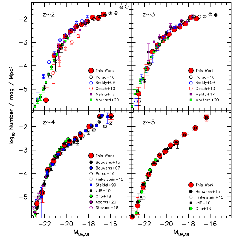
Figure 7.— Comparison of the new $z=2$-5 $UV$ LFs we derived updating and extending the redshift baseline of the Bouwens et al. (2015) and Bouwens et al. (2016: solid red circles) results against previous blank-field LF results in the literature including those from Reddy & Steidel (2009: open blue circles), Oesch et al. (2010: open red circles), Mehta et al. (2017: magenta solid squares), Parsa et al. (2016: black open circles), Moutard et al. (2020: solid green squares), Finkelstein et al. (2015: open gray circles), van den Bosch et al. (2010: black solid squares), Steidel et al. (1999: blue solid squares), Ono et al. (2018: solid green circles), Adams et al. (2018: solid violet circles), Stevans et al. (2018: open violet circles), and Bouwens et al. (2007: solid blue circles). The present determinations are in broad agreement with previous work. No results from lensing cluster studies are included here to keep the discussion simple, but will be included in a forthcoming companion paper focusing on the HFF clusters.

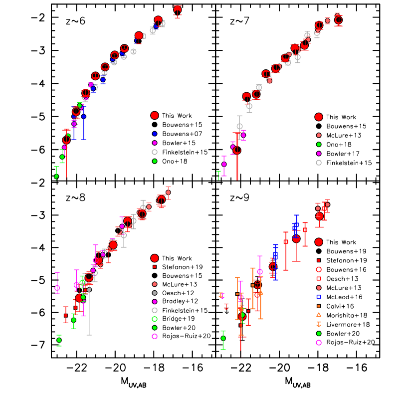
Figure 8.— Similar to Figure 7 but for our newly derived LFs at $z=6$-9. Included in these comparisons are the results of Bouwens et al. (2007: solid blue circles), Bouwens et al. (2015: solid black circles), Ono et al. (2018: solid green circles), Bowler et al. (2015: solid magenta circles), Finkelstein et al. (2015: open gray circles), McLure et al. (2013: solid light red circles), Bowler et al. (2017: solid magenta circles), Oesch et al. (2012: solid gray circles), Bradley et al. (2012: solid magenta circles), Bridge et al. (2019: open green circle), Bowler et al. (2020: green solid circles), Rojas-Ruiz et al. (2020: open magenta circles), Bouwens et al. (2019: solid black squares), Stefanon et al. (2019: solid red squares), Bouwens et al. (2016: open red circles), Oesch et al. (2013: open red squares), McLeod et al. (2016: open blue squares), Calvi et al. (2016: solid light red squares), Morishita et al. (2018: open red triangle), and Livermore et al. (2018: light red upper limits).

In making use of the search constraints to derive LF results, we only consider results to specific limiting magnitudes to avoid having the results be significantly impacted by uncertain completeness corrections or contamination rates. We adopt the same limiting magnitudes as Bouwens et al. (2015), except in the cases of the new samples considered here, including our $z\sim 2$-3 samples from the ERS, HDUV, and UVUDF data sets where 26.5 mag, 28.0 mag, and 29.0 mag, respectively, our $z\sim 4$-9 HFF parallel samples where 29.0 mag limits are used, and our new $z\sim 9$ XDF, HUDF09-1, and HUDF09-2 samples where 30.0, 29.0, and 29.0 mag, respectively, are used.

Finally, over the HFF parallel fields, we accounted for the estimated magnification factors using the lensing models from Merten (2016). The approximate lensing magnification that we applied in magnitudes for each parallel field is provided in Table 3 for sources at $z\sim 6$. The magnification factors at other redshifts are very similar. The search volumes and luminosities were reduced and scaled according to the lensing magnification in each field.

We present updated stepwise determinations of the $UV$ LF at $z\sim 2$, $z\sim 3$, $z\sim 4$, $z\sim 5$, $z\sim 6$, $z\sim 7$, $z\sim 8$, and $z\sim 9$ in Figure 5 and Table 4, along with the new $z\sim 10$ results from Oesch et al. (2018a) designed to complement this study. $UV$ LF results are similarly derived using a Schechter parameterization by first fitting for the shape of the LF as in the SWML approach as in Sandage et al. (1979) and then determining the normalization $\phi^{*}$. The best-fit Schechter results are provided in Table 5, together with the $z\sim 10$ results of Oesch et al. (2018a). For our $z\sim 9$ LF determinations, we fix the characteristic luminosity $M^{*}$ to the value implied by the fitting formula derived in §4.2, i.e., $-$21.15 mag. For the Oesch et al. (2018a) $z\sim 10$ LF constraints, we similarly fixed $M^{*}$ to be $-21.19$ mag, while fitting for constraints on $\phi^{*}$ and $\alpha$.

Included in our best-fit LFs are the quoted stepwise constraints from a large variety of different ground-based probes including Stefanon et al. (2019), Bowler et al. (2015), and the brightest two magnitude bins in Bowler et al. (2015) where their selection of bright $z\sim 7$ galaxies should be the most complete.

Finally, the new constraints on the UV LF at $z\sim 6$ and $z\sim 7$ faintward of $-$23 mag from Ono et al. (2018) are included in our fits. If constraints brighter than $-$23 mag are included in our $UV$ LF fits, we find that the LF constraints are not well represented by a Schechter function-type form and the characteristic luminosity is driven towards higher values.

Figure 6 shows the 68% and 95% confidence intervals we compute for various two-dimentional projections of the Schechter parameters. We discuss evolution in the Schechter parameters in §4.2.

4. Discussion

4.1. Comparison with Previous LF Results

There is now a quite substantial body of work on the $UV$ LF at high redshift, from $z\sim 2$-3 (Madau et al. 1996; Steidel et al. 1999; Reddy & Steidel 2009; Oesch et al. 2010; Alavi et al. 2016) to $z\sim 4$-5 (e.g., Bouwens et al. 2007; van der Berg et al. 2010; Bouwens et al. 2015; Parsa et al. 2016) to $z\sim 6$-10 (Bouwens et al. 2008; Oesch et al. 2010, 2012; McLure et al. 2013; Schenker et al. 2013; Bouwens et al. 2015, 2016, 2017; Finkelstein et al. 2015; Oesch et al. 2015; McLeod et al. 2016; Livermore et al. 2018; Atek et al. 2018).

It is useful to compare the present determinations of the $UV$ LFs against many previous determinations to quantify possible differences in the results. Given that the present results utilize blank-field surveys to arrive at the LFs results, we focus on comparisons with previous blank-field determinations to keep the comparisons most direct.

Accordingly, in Figures 7 and 8, we provide a comprehensive set of comparisons of our new $z=2$-9 LF results from the HFFs with a variety of noteworthy previous work, including Steidel et al. (1999), Bouwens et al. (2007), Reddy & Steidel (2009), Oesch et al. (2010), van der Berg et al. (2010), Bradley et al. (2012), Oesch et al. (2012), McLure et al. (2013), Bouwens et al. (2015), Bowler et al. (2015), Finkelstein et al. (2015), Bouwens et al. (2016), Parsa et al. (2016), Bouwens et al. (2016), McLeod et al. (2016), Ono et al. (2018), and Stefanon et al. (2019).

We consider the redshift intervals in turn, below:

$z\sim 2$-3: For $UV$ luminosities of $\sim$0.1 $L^{*}$ ($-$20 mag to $-$17 mag), most existing LF results at $z\sim 2$ and $z\sim 3$ are broadly in agreement. This is especially true brightward of $-$20, where essentially all recent studies (this study; Reddy & Steidel 2009; Oesch et al. 2010; Parsa et al. 2016; Mehta et al. 2017; Moutard et al. 2020) show approximately (modulo $<$0.2-mag differences) the same bright-end cut-off. In contrast to the $z\sim 3$ results, the absolute magnitude of the cut-off at $z\sim 2$ varies much more substantially, occurring$\sim$0.7 mag brighter in the Reddy & Steidel (2009) case than in the Oesch et al. (2010) case.

The only apparent exception to this are the $z\sim 2$ results of Oesch et al. (2010), which appear to be a factor of $\sim 3$ lower than the other $z\sim 2$ LF results. To investigate this difference, we constructed a $z\sim 1.9$ sample of galaxies using the same $U_{275}$-dropout criteria as given in Oesch et al. (2010) and compared it to the present selection of $z\sim 2$ galaxies to the same 25.5-mag limit in the $B_{435}$ band. Our $z\sim 2$ selection shows $\sim$2.5$\times$ more sources, i.e., 245, to the same magnitude limit as Oesch et al. (2010) use. If the estimate of the selection volume at $z\sim 2$ in these previous studies is similar to the present estimate, this would largely explain the difference in our LF results. While the Oesch et al. (2010) results seem very reasonable in isolation, the estimated selection volume in $z\sim 2$ samples is very sensitive to the expected S/N in the $U_{275}$ and $U_{336}$ bands, which in turn is sensitive to the source size and surface brightness. Additionally, a difference in the mean redshift of the Oesch et al. (2010) $z\sim 1.9$ election and the present selection $z\sim 2.1$ (typical redshift uncertainties for sources is $\Delta z\sim 0.2$-0.3) likely contribute to the observed differences.

$z\sim 4$-5: For comparisons between our new $z\sim 4$ and $z\sim 5$ results and previous determinations, we note good agreement between our new $z\sim 4$ and $z\sim 5$ LF determinations and various comparison luminosity functions from the literature (Figure 7: Steidel et al. 1999; van der Berg et al. 2010; Bouwens et al. 2015; Finkelstein et al. 2015; Parsa et al. 2016; Ono et al. 2018; Stevans et al. 2018; Adams et al. 2020) at the high luminosity end. At lower luminosities, i.e., reaching to $-17$ to $-16$ mag, our $z\sim 4$ LF determinations are in good agreement with our previous determinations (Bouwens et al. 2007, Bouwens et al. 2015) but a factor of 1.5-2 higher than those in Finkelstein et al. (2015) and Parsa et al. (2016). One potential explanation for the difference could be Finkelstein et al. (2015) and Parsa et al. (2016)’s use of a $1/V_{max}$ estimator to derive the Schechter function parameters. LF determinations using the $1/V_{max}$ estimator can be impacted if the search fields probing a particular luminosity range show a significant overdensity or underdensity of sources. In the case of the HUDF/XDF, our best-fit $z\sim 4$ LF determination suggests we would find 40$\pm$7% more $z\sim 4$ sources in the HUDF/XDF data than what we actually find, suggesting that the HUDF/XDF region may be underdense by $\sim$30%. If the Finkelstein et al. (2015)/Parsa et al. (2016) determinations are impacted by this issue, it could result in $\Delta\alpha\sim-0.1$ shallower values for the faint-end slope $\alpha$, consistent with the observed differences.

$z\sim 6$-7: As at $z\sim 4$-5, our new constraints on the $UV$ LFs at $z\sim 6$-7 are in broad agreement (Figure 7) with previous determinations, e.g., Bouwens et al. (2007), McLure et al. (2013), Bouwens et al. (2015), Bowler et al. (2015), Ono et al. (2018), and Finkelstein et al. (2015). At intermediate luminosities, i.e., $-19$ mag, where the results would be sensitive to the faintest sources in the CANDELS selections and the estimated selection volumes, the Finkelstein et al. (2015) $z\sim 6$ LF results (and to lesser extent their $z\sim 7$ results) are a factor of $\sim$2 lower than our new and previous LF results. If the selection volumes in this regime were overestimated due to reliance on the selected population of $z\sim 6$ galaxies from CANDELS (which would tend to include only the highest surface brightness sources) for the completeness estimates, this could explain the differences at $\sim$$-$19 mag. In any case, at $z\sim 6$-7, we consistently recover the same volume density of sources at $-19$ mag regardless of whether we rely on the significantly deeper HFF or CANDELS data.

$z\sim 8$-9: Our new results at $z\sim 8$-9 are in excellent agreement with essentially all of the latest determinations at these redshifts (Oesch et al. 2012, 2013; Bradley et al. 2012; McLure et al. 2013; Bouwens et al. 2015, 2016, 2019; Finkelstein et al. 2015; Calvi et al. 2016; McLeod et al. 2016; Morashita et al. 2018; Livermore et al. 2018; Bridge et al. 2019; Bowler et al. 2020; Rojas-Ruiz et al. 2020). At the bright end, the new $z\sim 8$-9 LF constraints from Stefanon et al. (2019: see also Stefanon et al. 2017b) and Bowler et al. (2020) from very wide-area ($\sim 2$-6 deg²) searches are consistent with what we derive, but extend to higher luminosities. While the Calvi et al. (2016) results from the BoRG/HIPPIES pure-parallel fields are somewhat in excess of our own, this is without inclusion of the Spitzer/IRAC observations into the analysis to exclude lower-redshift interlopers and AGN. The Morishita et al. (2018) analyses of the BoRG/HIPPIES fields are in much better agreement with our results, supporting this conclusion. The $z\sim 8$ LF from Rojas-Ruiz et al. (2018) at $-$23 mag is clearly higher than the other LF determinations that probe this regime (Stefanon et al. 2019; Bowler et al. 2020), but is based on only a single source and therefore the uncertainties are large. At fainter luminosities, the faint-end results from McLure et al. (2018) and McLeod et al. (2016) are also encouragingly consistent with the new LF results we have obtained including all six parallel fields in the HFF program.

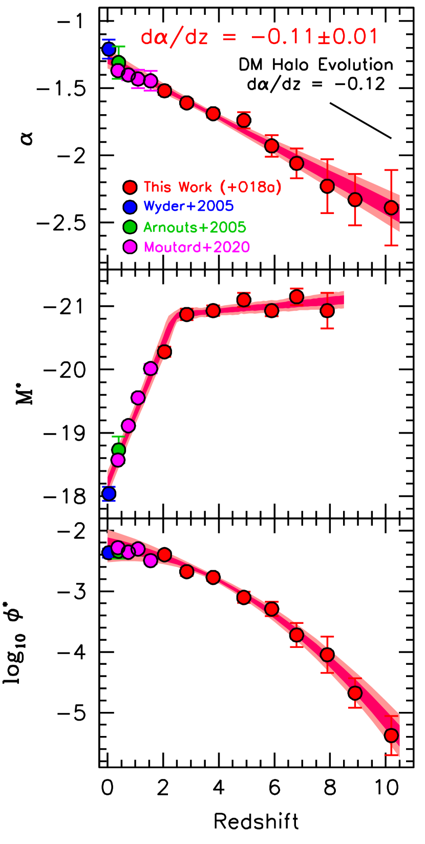
Figure 9.— Determinations of the faint-end slope $\alpha$, characteristic luminosity $M^{*}$, and normalization $\phi^{*}$ to the $UV$ LF derived at $z=2$-10 in this work and Oesch et al. (2018a: O18a) from blank-field observations alone (solid red circles). The plotted $z\sim 2$-3 determinations are our new results derived using the HDUV+UVUDF+ERS WFC3/UVIS data sets, while the plotted $z\sim 4$-9 results represent updates to our earlier determinations from Bouwens et al. (2015, 2016) including new constraints from the HFF-parallel fields. The Wyder et al. (2005) faint-end slope determination at $z\sim 0.055$ is shown, an average of the $z\sim 0.2$-0.4 determinations by Arnouts et al. (2005), and the $z=0.3$-0.45, $z=0.6$-0.9, $z=0.9$-1.3, and $z=1.3$-1.8 determinations of Moutard et al. (2020). The light and dark reddish magenta contours show our 68% and 95% constraints on the evolution in the faint-end slope $\alpha$, $M^{*}$, and $\log_{10}\phi^{*}$ inferred from a fit to the present LF results. The plotted $z<3$ constraints on $M^{*}$ from Wyder et al. (2005), Arnouts et al. (2005), and Moutard et al. (2020) are used in deriving the best-fit relations. The present fits represent an update to the determinations in Parsa et al. (2016) who look at the evolution of the LF parameters over a similar redshift baseline (see also Moutard et al. 2020, Bowler et al. 2020, and Finkelstein 2016). Interestingly, the observed evolution can be remarkably well explained by the predicted evolution in the halo mass function and a fixed star-formation efficiency model (see §4.2).

4.2. Evolution in $\alpha$, $M^{*}$, and $\phi^{*}$

As in our previous comprehensive analyses of the $UV$ LF at $z\sim 4$-10 based on blank-field observations (Bouwens et al. 2015), we can use our improved constraints on the $UV$ LF to examine evolution in the Schechter parameters.

While the evolution in these quantities is already clear based on previous work (e.g., Bouwens et al. 2015; Bowler et al. 2015; Finkelstein et al. 2015), the new observations allow us to improve our previous determinations even further to map out the evolutionary trends. While recognizing the value of $UV$ LF results that rely on lensing magnification by galaxy clusters, we intentionally do not include them in the present determinations to avoid any systematics that might result from managing uncertainties in the lensing models or uncertainties in the sizes of the lowest luminosity sources.

While our primary interest here is in looking at the faint-end slope trend, we will also look at how the other two Schechter parameters evolve. Based on the plotted contours in Figure 6, the normalization $\phi^{*}$ shows a similarly smooth increase with cosmic time, while the faint-end slope $\alpha$ shows a smooth evolution from very steep values to shallower values at later points in cosmic time.

As in our previous work, e.g., Bouwens et al. (2008), we assume that the evolution is linear in $\alpha$ and $M^{*}$, but will take the evolution in $\log_{10}\phi^{*}$ to be quadratic in form. To account for impact of quenching on the high star formation end of the main sequence (e.g., Ilbert et al. 2013; Muzzin et al. 2013), we allow for a break in the linear evolution of the $UV$ LF at $z\lesssim 2.5$, fitting separately for the transition redshift $z_{t}$ and linear trend at $z\lesssim 2.5$. In fitting for the trend in the characteristic luminosity, we make use of the Wyder et al. (2005) UV LF results at $z\sim 0.055$, the Arnouts et al. (2005) results at $z\sim 0.3$, and the Moutard et al. (2020) results over the redshift range $z\sim 0.3$-1.8.

The best-fit evolution we derive based on our blank-field LF results at $z\sim 2$-10 is the following:

$$M_{UV}^{*}= \left\{\begin{array}[]{ll}(-20.89\pm 0.12)+&\textrm{for}~{}z<z_{t}\\ (-1.09\pm 0.07)(z-z_{t}),\\ (-21.03\pm 0.04)+&\textrm{for}~{}z>z_{t}\\ (-0.04\pm 0.02)(z-6),\end{array}\right.$$

$$\phi^{*}= (0.40\pm 0.04)(10^{-3}\textrm{Mpc}^{-3})~{}~{}~{}~{}~{}~{}~{}~{}~{}~{}~{}$$

$$~{}~{}10^{(-0.33\pm 0.02)(z-6)+(-0.024\pm 0.006)(z-6)^{2}}$$

$$\alpha= (-1.94\pm 0.03)+(-0.11\pm 0.01)(z-6)$$

where $z_{t}=2.46\pm 0.11$. A comparison of the best-fit trends with the derived Schechter parameters for the $UV$ LF from $z\sim 2$ to $z\sim 10$ is presented in Figure 9.

As in previous work, the faint-end slope $\alpha$ of the $UV$ LF is well described by a linear flattening in $\alpha$ from $\alpha\sim-2.3$ at $z\sim 8$-10 to significantly shallower slopes, i.e., $\alpha\sim-1.5$, at $z\sim 2$. Moreover, an extrapolation of our results to $z\sim 0$ agree very well with the results obtained by Wyder et al. (2005) at $z\sim 0.055$, Arnouts et al. (2005) at $z\sim 0.3$, and Moutard et al. (2020) over the redshift range $z\sim 0.3$-1.8.

The observed change in $\alpha$ with redshift we find, i.e., $d\alpha/dz=-0.11\pm 0.01$ is very similar with predicted flattening based on the evolution in the halo mass function. Bouwens et al. (2015) find that $d\alpha/dz=-0.12$ purely due to a flattening in halo mass function with cosmic time using a simple conditional luminosity function model. Amazingly, the faint-end slope $\alpha$ appears to maintain a roughly linear relationship with redshift down to $z\sim 0$. At first glance, this might seem surprising given the increasing importance of other physical processes like AGN feedback (e.g., Scannapieco & Oh 2004; Croton et al. 2006) and the potential impact of this feedback on star formation in lower mass halos. The trends we find here are very similar to what we reported in our earlier LF study (Bouwens et al. 2015), i.e., $d\alpha/dz=-0.10\pm 0.03$, and also similar to the $d\alpha/dz\sim-0.11$ trend Parsa et al. (2016) and Finkelstein (2016) find fitting the then-available LF constraints in the literature.

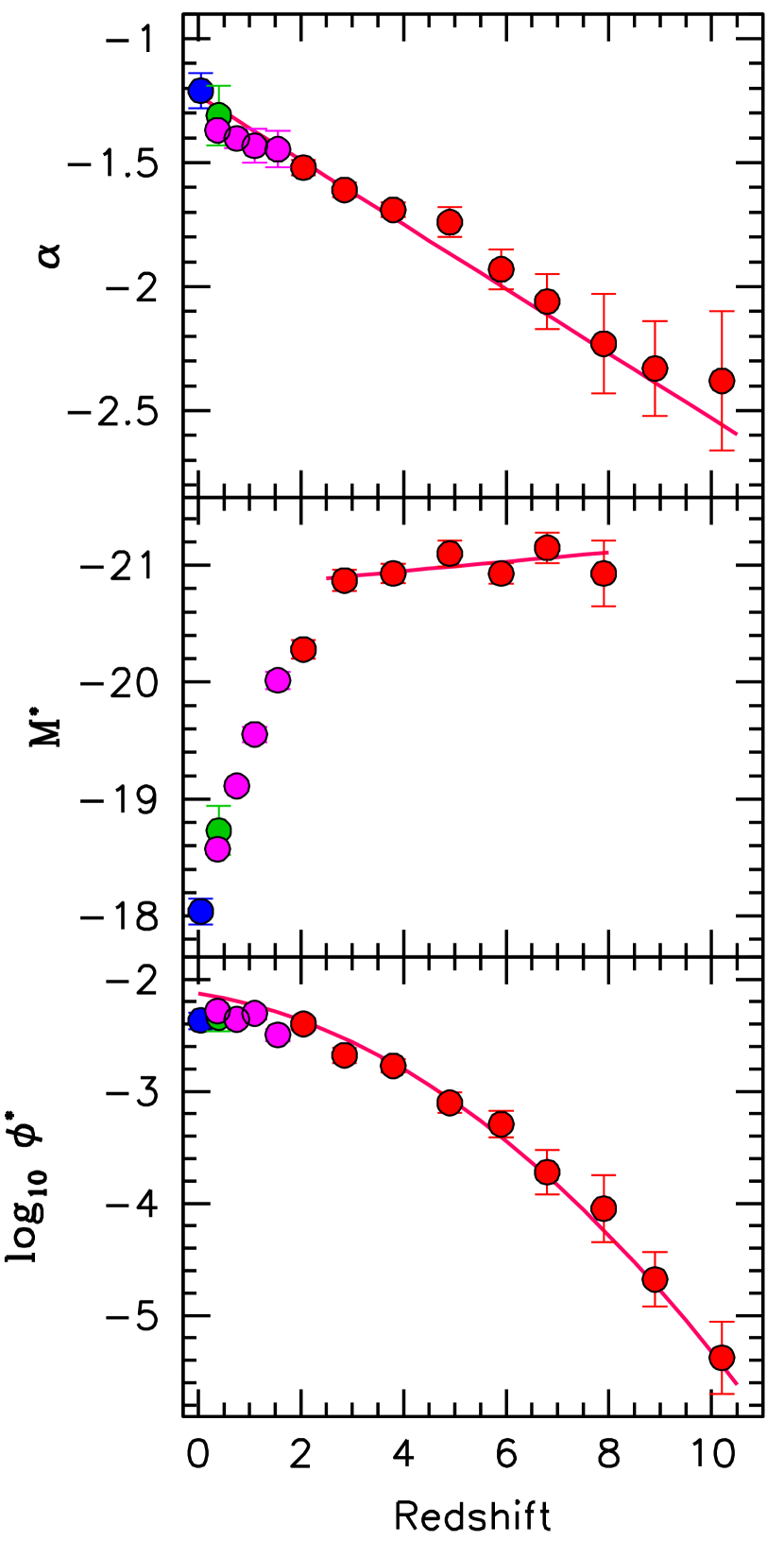
Figure 10.— Comparison of the observational constraints presented in Figure 9 with the predictions (red lines) of the simple constant star formation efficiency model presented in Appendix I of Bouwens et al. (2015), while keeping the characteristic luminosity $M^{*}$ fixed to the $-21.03-0.04(z-6)$ mag parameterization derived from our empirical fits (§4.2). It is striking how observational results agree with the dependence predicted using the evolution of the halo mass function and a simple constant star formation efficiency model.

The characteristic luminosity $M^{*}$ maintains a relatively fixed value of $-21.02$ mag over the redshift range $z\sim 8$ to $z\sim 3$. The best-fit dependence of $M^{*}$ on redshift is $-0.04\pm 0.02$ and nominally significant at $2\sigma$. As has been argued by Bouwens et al. (2009) and Reddy et al. (2010), the observed exponential cut-off at the bright end of the $UV$ LF likely occurs due to the impact of dust extinction in sources with the highest masses and SFRs. Galaxies with masses and SFRs higher than some critical value (e.g., Spitler et al. 2014; Stefanon et al. 2017b) tend to suffer sufficient attenuation that these sources actually become fainter in the rest-$UV$ than lower mass, lower SFR sources. The critical $UV$ luminosity where the UV luminosity vs. SFR relationship transitions from being positively correlated to negative correlatively appears to set the value of the characteristic luminosity (e.g., Bouwens et al. 2009; Reddy et al. 2010). The relatively minimal evolution in the characteristic luminosity $M^{*}$ with redshift suggests that this critical SFR does not evolve dramatically with redshift, as Bouwens et al. (2015) illustrate with the conditional luminosity function model they present in their §5.5.2 and Figure 20.

The normalization $\phi^{*}$ of the $UV$ LF increases monotonically with cosmic time from $z\sim 10$ to $z\sim 2$, with a steeper dependence on redshift from $z\sim 10$ to $z\sim 7$ than from $z\sim 7$ to $z\sim 2$. We found that the dependence of $\log_{10}\phi^{*}$ with redshift could be well described by a second-order polynomial. The amplitude of the second-order term, i.e., $-0.024\pm 0.006$, is significant at 4$\sigma$. The change in the dependence of $\log_{10}\phi^{*}$ with redshift has been previous framed as “accelerated” evolution by Oesch et al. (2012). Analyses of subsequent observations in Oesch et al. (2014), Oesch et al. (2018a), and Ishigaki et al. (2018: but see also McLeod et al. 2016) provide further evidence for this result.

The observed evolution can fairly naturally be explained, using a constant star formation efficiency model, by the evolution of the halo mass function (e.g., Bouwens et al. 2008; Tacchella et al. 2013; Bouwens et al. 2015; Mason et al. 2015; Oesch et al. 2018; Harikane et al. 2018; Tacchella et al. 2018). Oesch et al. (2018), for example, showed with such a model that one could reproduce the observed evolution in the dust-corrected UV luminosity from $z\sim 10$ to $z\sim 4$. Adopting the conditional LF model from Bouwens et al. (2015: their Appendix I), fixing the characteristic luminosity $M^{*}$ to $\sim-21.03$ mag preferred from our empirical fitting formula, and fitting for $\phi^{*}$ and $\alpha$, we find a best-fit parameterization for $\phi^{*}$ of (0.00036 Mpc^-3) $10^{-0.34(z-6)-0.024(z-6)^{2}}$, remarkably similar to the coefficients we recovered in deriving the LF fitting formula from the observations. In deriving Schechter parameters from the model LF results from Bouwens et al. (2015), we minimized the square logarithmic difference between the condition LF predictions and the Schechter function fits over the range $-22$ to $-15$.

Fixing the characteristic luminosity $M^{*}$ instead to that found in our fitting formula, i.e., $-21.03-0.04(z-6)$ mag, we find a best-fit parameterization for $\phi^{*}$ of (0.00036 Mpc^-3) $10^{-0.37(z-6)-0.025(z-6)^{2}}$. This confirms that constant star formation efficiency models do clearly predict a second-order dependence in the Schechter parameters, i.e., “acceleration,” vs. redshift. In Figure 10, we compare the predictions of this simple model with the observational results, and it is striking how well the evolutionary trends of such a model agrees with the observations. This strongly suggests that much of the evolution of the $UV$ LF can be explained by largely explained by the evolution of the halo mass function and an unevolved star formation efficiency.

Given our reliance on what is currently the largest HST sample of $z=2$-10 galaxy candidates to date, our derived evolutionary trends arguably represent the most accurate determinations obtained to date.

5. Summary

In this paper, we make use of a suite of new data sets to significantly expand current HST samples of $z\sim 2$-9 galaxies and to improve recent determinations of the $UV$ LF based on HST data.

For our $z\sim 2$-3 selections, the most important new data set are the HDUV observations in the F275W and F336W bands over a $\sim$94 arcmin² area at $\sim$0.28$\mu$m and 0.34$\mu$m. By combining this data set with the $\sim$50 arcmin² WFC3/UVIS ERS (Windhorst et al. 2011) and $\sim$7 arcmin² UVUDF (Teplitz et al. 2013) data, we use a total search area of $\sim$150 arcmin² to construct samples of $z\sim 2$-3 galaxies.

By combining these data with the optical and near-IR data over the GOODS North and South fields, we are able to construct a sample of 12098 galaxies in the redshift range $z\sim 2$-3. This is $>$10$\times$ larger than the samples of $z\sim 2$-3 galaxies that Hathi et al. (2010), Oesch et al. (2010), and Mehta et al. (2017) had available with HST in earlier determinations of the $UV$ LF at $z\sim 2$-3.

For our $z\sim 4$-9 selections, the most noteworthy new data are the HST optical and near-IR observations obtained over the six parallel fields from the Hubble Frontier Fields program (Lotz et al. 2017). Those observations probe galaxies to $UV$ luminosities of $\sim$0.08 $L_{z=3}^{*}$ and are only exceeded by the HUDF in terms of their sensitivity. From the six parallel fields to the HFF clusters, we identify 1381 $z\sim 4$, 448 $z\sim 5$, 209 $z\sim 6$, 122 $z\sim 7$, 34 $z\sim 8$, and 13 $z\sim 9$ galaxies, respectively. Combining these samples with those from Bouwens et al. (2015), there are $>$12,000 sources in our HST-based field samples.

All together and including the $z\sim 10$-11 selection from Oesch et al. (2018a), our selections of $z=2$-11 galaxies from HST fields include 24741 galaxies. This is more than twice the number of sources as the largest previous samples of galaxies over this redshift range.

We leverage the present, even larger samples of $z=2$-9 galaxies to construct new and improved determinations of the $UV$ LFs at $z\sim 2$-9. The present determinations constitute the best blank-field LF results to date. Encouragingly enough, our new determinations are in excellent agreement with most previous determinations where they overlap.

Combining new LF results with the $z\sim 10$ LF result from Oesch et al. (2018a), we are in position to reassess the evolution derived in a self-consistent way, particularly in terms of known Schechter function parameters like the faint-end slope $\alpha$ and the normalization $\phi^{*}$ of the LF.

As in previous studies, we find that the faint-end slope $\alpha$ steepens towards high redshift at approximately a fixed rate vs. redshift (e.g., Bouwens et al. 2015; Parsa et al. 2016; Finkelstein 2016). The observed evolution appears to be almost identical to what would expect, i.e., $d\alpha/dz\sim-0.12$ based on changes to the slope of the halo mass function across the observed redshift range (e.g., Bouwens et al. 2015).

We find that the characteristic luminosity $M^{*}$ remains relatively fixed at $\sim-21.02$ mag over the redshift range $z\sim 8$ to $z\sim 3$ (see also e.g., Bouwens et al. 2015; Bowler et al. 2015; Finkelstein et al. 2015), but becomes increasingly fainter at $z\lesssim 2.5$ where quenching becomes important (e.g., Scannapieco et al. 2005; Peng et al. 2010). The presence of an exponential cut-off in the $UV$ LF at $z\gtrsim 3$ is thought to be imposed by the presence of dust extinction (e.g., Bouwens et al. 2009; Reddy et al. 2010), with the characteristic luminosity set by the $UV$ luminosities where the increased dust extinction in galaxies more than offsets increases in the SFRs in galaxies. The absence of strong evolution in $M^{*}$ suggests a similar lack of evolution in this transition SFR or $UV$ luminosity.

Finally, we find a systematic decrease in the normalization $\phi^{*}$ of the $UV$ LF towards high redshift (e.g., McLure et al. 2010; Bouwens et al. 2015). $\log_{10}$ $\phi^{*}$ can be well described by quadratic relationship in redshift, with a significantly flatter relationship at $z<7$ than it is at $z>7$, consistent with the conclusions from studies favoring “accelerated” evolution at $z>8$ (Oesch et al. 2012, 2018a). Interestingly, using the constant star formation efficiency conditional luminosity function model from Bouwens et al. (2015: their Appendix I), we find that we can reproduce the observed evolution in $\phi^{*}$ remarkably well (as shown in Figure 10). Similar to our discussion in Bouwens et al. (2015), consistency of the $UV$ LF results with fixed star formation efficiency models has also been argued in Oesch et al. (2018) and Tacchella et al. (2018). Again, this demonstrates that much of the evolution in the $UV$ LF (from $z\sim 10$ to $z\sim 2.5$ at least) can be explained by the evolution in the halo mass function and a simple fixed star formation efficiency model.

In a follow-up paper, we will be revisiting the present constraints on the $UV$ LF at $z\sim 2$-9 by incorporating constraints available from the HFF lensing cluster observations. With lensing cluster observations, we will show that we can obtain a completely consistent constraints on the Schechter parameters using the lensing cluster data alone or in combination with the field constraints.

References

- Adams et al. (2020) Adams, N. J., Bowler, R. A. A., Jarvis, M. J., et al. 2020, MNRAS, 494, 1771
- Aihara et al. (2018) Aihara, H., Arimoto, N., Armstrong, R., et al. 2018a, PASJ, 70, S4
- Aihara et al. (2018) Aihara, H., Armstrong, R., Bickerton, S., et al. 2018b, PASJ, 70, S8
- Alavi et al. (2016) Alavi, A., Siana, B., Richard, J., et al. 2016, ApJ, 832, 56
- Anderson & Bedin (2010) Anderson, J., & Bedin, L. R. 2010, PASP, 122, 1035
- Arnouts et al. (2005) Arnouts, S., Schiminovich, D., Ilbert, O., et al. 2005, ApJ, 619, L43
- Atek et al. (2018) Atek, H., Richard, J., Kneib, J.-P., & Schaerer, D. 2018, MNRAS, 479, 5184
- Beckwith et al. (2006) Beckwith, S. V. W., Stiavelli, M., Koekemoer, A. M., et al. 2006, AJ, 132, 1729
- Behroozi et al. (2013) Behroozi, P. S., Wechsler, R. H., & Conroy, C. 2013, ApJ, 770, 57
- Bertin and Arnouts (1996) Bertin, E. and Arnouts, S. 1996, A&AS, 117, 39
- Bouwens, Broadhurst and Silk (1998) Bouwens, R., Broadhurst, T. and Silk, J. 1998, ApJ, 506, 557
- Bouwens et al. (2003) Bouwens, R., Broadhurst, T., & Illingworth, G. 2003a, ApJ, 593, 640
- Bouwens et al. (2007) Bouwens, R. J., Illingworth, G. D., Franx, M., et al. 2007, ApJ, 670, 928
- Bouwens et al. (2008) Bouwens, R. J., Illingworth, G. D., Franx, M., & Ford, H. 2008, ApJ, 686, 230
- Bouwens et al. (2009) Bouwens, R. J., Illingworth, G. D., Franx, M., et al. 2009, ApJ, 705, 936
- Bouwens et al. (2010) Bouwens, R. J., Illingworth, G. D., González, V., et al. 2010, ApJ, 725, 1587
- Bouwens et al. (2011) Bouwens, R. J., Illingworth, G. D., Oesch, P. A., et al. 2011, ApJ, 737, 90
- Bouwens et al. (2015) Bouwens, R. J., Illingworth, G. D., Oesch, P. A., et al. 2015, ApJ, 803, 34
- Bouwens (2015) Bouwens, R. 2015, HST Proposal, 14459
- Bouwens et al. (2016) Bouwens, R. J., Aravena, M., Decarli, R., et al. 2016a, ApJ, 833, 72
- Bouwens et al. (2016) Bouwens, R. J., Oesch, P. A., Labbé, I., et al. 2016b, ApJ, 830, 67
- Bouwens et al. (2017) Bouwens, R. J., Oesch, P. A., Illingworth, G. D., et al. 2017b, ApJ, 843, 129
- Bouwens et al. (2019) Bouwens, R. J., Stefanon, M., Oesch, P. A., et al. 2019, ApJ, 880, 25
- Bowler et al. (2015) Bowler, R. A. A., Dunlop, J. S., McLure, R. J., et al. 2015, MNRAS, 452, 1817
- Bowler et al. (2020) Bowler, R. A. A., Jarvis, M. J., Dunlop, J. S., et al. 2020, MNRAS, 493, 2059
- Bradley et al. (2012) Bradley, L. D., Trenti, M., Oesch, P. A., et al. 2012, ApJ, 760, 108
- Brammer et al. (2008) Brammer, G. B., van Dokkum, P. G., & Coppi, P. 2008, ApJ, 686, 1503
- Bridge et al. (2019) Bridge, J. S., Holwerda, B. W., Stefanon, M., et al. 2019, ApJ, 882, 42
- Capak et al. (2007) Capak, P., Aussel, H., Ajiki, M., et al. 2007, ApJS, 172, 99
- Croton et al. (2006) Croton, D. J., Springel, V., White, S. D. M., et al. 2006, MNRAS, 365, 11
- Davidzon et al. (2017) Davidzon, I., Ilbert, O., Laigle, C., et al. 2017, A&A, 605, A70
- Dressel et al. (2012) Dressel, L., et al. 2012. “Wide Field Camera 3 Instrument Handbook, Version 5.0” (Baltimore: STScI)
- Efstathiou et al. (1988) Efstathiou, G., Ellis, R. S., & Peterson, B. A. 1988, MNRAS, 232, 431
- Ellis et al. (2013) Ellis, R. S., McLure, R. J., Dunlop, J. S., et al. 2013, ApJ, 763, L7
- Finkelstein et al. (2013) Finkelstein, S. L., Papovich, C., Dickinson, M., et al. 2013, Nature, 502, 524
- Finkelstein et al. (2014) Finkelstein, S. L., Ryan, R. E., Jr., Papovich, C., et al. 2015, 810, 71
- Grogin et al. (2011) Grogin, N. A., Kocevski, D. D., Faber, S. M., et al. 2011, ApJS, 197, 35
- Harikane et al. (2016) Harikane, Y., Ouchi, M., Ono, Y., et al. 2016, ApJ, 821, 123
- Harikane et al. (2018) Harikane, Y., Ouchi, M., Ono, Y., et al. 2018, PASJ, 70, S11
- Hashimoto et al. (2018) Hashimoto, T., Laporte, N., Mawatari, K., et al. 2018, Nature, 557, 392
- Hathi et al. (2010) Hathi, N. P., Ryan, R. E., Jr., Cohen, S. H., et al. 2010, ApJ, 720, 1708
- Ilbert et al. (2013) Ilbert, O., McCracken, H. J., Le Fèvre, O., et al. 2013, A&A, 556, A55
- Illingworth et al. (2013) Illingworth, G. D., Magee, D., Oesch, P. A., et al. 2013, ApJS, 209, 6
- Illingworth et al. (2016) Illingworth, G., Magee, D., Bouwens, R., et al. 2016, arXiv:1606.00841
- Ishigaki et al. (2018) Ishigaki, M., Kawamata, R., Ouchi, M., et al. 2018, ApJ, 854, 73
- Koekemoer et al. (2011) Koekemoer, A. M., Faber, S. M., Ferguson, H. C., et al. 2011, ApJS, 197, 36
- Koekemoer et al. (2013) Koekemoer, A. M., Ellis, R. S., McLure, R. J., et al. 2013, ApJS, 209, 3
- Koekemoer et al. (2014) Koekemoer, A. M., Avila, R. J., Hammer, D., et al. 2014, American Astronomical Society Meeting Abstracts #223
- Kron (1980) Kron, R. G. 1980, ApJS, 43, 305
- Labbé et al. (2006) Labbé, I., Bouwens, R., Illingworth, G. D., & Franx, M. 2006, ApJ, 649, L67
- Labbé et al. (2010) Labbé, I., González, V., Bouwens, R. J., et al. 2010a, ApJ, 708, L26
- Labbé et al. (2010) Labbé, I., González, V., Bouwens, R. J., et al. 2010b, ApJ, 716, L103
- Labbé et al. (2013) Labbé, I., Oesch, P. A., Bouwens, R. J., et al. 2013, ApJ, 777, L19
- Labbé et al. (2015) Labbé, I., Oesch, P. A., Illingworth, G. D., et al. 2015, ApJS, 221, 23
- Leja et al. (2019) Leja, J., Johnson, B. D., Conroy, C., et al. 2019, ApJ, 877, 140
- Livermore et al. (2018) Livermore, R. C., Trenti, M., Bradley, L. D., et al. 2018, ApJ, 861, L17
- Lotz et al. (2017) Lotz, J. M., Koekemoer, A., Coe, D., et al. 2017, ApJ, 837, 97
- Madau et al. (1996) Madau, P., Ferguson, H. C., Dickinson, M. E., et al. 1996, MNRAS, 283, 1388
- Madau & Dickinson (2014) Madau, P., & Dickinson, M. 2014, ARA&A, 52, 415
- Magee et al. (2011) Magee, D. K., Bouwens, R. J., & Illingworth, G. D. 2011, Astronomical Data Analysis Software and Systems XX, 442, 395
- Mason et al. (2015) Mason, C. A., Trenti, M., & Treu, T. 2015, ApJ, 813, 21
- McLeod et al. (2016) McLeod, D. J., McLure, R. J., & Dunlop, J. S. 2016, MNRAS, 459, 3812
- McLure et al. (2013) McLure, R. J., Dunlop, J. S., Bowler, R. A. A., et al. 2013, MNRAS, 432, 2696
- Mehta et al. (2017) Mehta, V., Scarlata, C., Rafelski, M., et al. 2017, ApJ, 838, 29
- Merlin et al. (2016) Merlin, E., Amorín, R., Castellano, M., et al. 2016, A&A, 590, A30
- Morishita et al. (2018) Morishita, T., Trenti, M., Stiavelli, M., et al. 2018, ApJ, 867, 150
- Moutard et al. (2020) Moutard, T., Sawicki, M., A rnouts, S., et al. 2020, MNRAS, 494, 1894
- Muzzin et al. (2013) Muzzin, A., Marchesini, D., Stefanon, M., et al. 2013, ApJ, 777, 18
- Oesch et al. (2010) Oesch, P. A., Bouwens, R. J., Carollo, C. M., et al. 2010, ApJ, 725, L150
- Oesch et al. (2012) Oesch, P. A., Bouwens, R. J., Illingworth, G. D., et al. 2012, ApJ, 745, 110
- Oesch et al. (2013) Oesch, P. A., Bouwens, R. J., Illingworth, G. D., et al. 2013, ApJ, 773, 75
- Oesch et al. (2014) Oesch, P. A., Bouwens, R. J., Illingworth, G. D., et al. 2014, ApJ, 786, 108
- Oesch et al. (2018) Oesch, P. A., Bouwens, R. J., Illingworth, G. D., Labbé, I., & Stefanon, M. 2018a, ApJ, 855, 105
- Oesch et al. (2018) Oesch, P. A., Montes, M., Reddy, N., et al. 2018b, ApJS, 237, 12
- Oke & Gunn (1983) Oke, J. B., & Gunn, J. E. 1983, ApJ, 266, 713
- Ono et al. (2012) Ono, Y., Ouchi, M., Mobasher, B., et al. 2012, ApJ, 744, 83
- Ono et al. (2018) Ono, Y., Ouchi, M., Harikane, Y., et al. 2018, PASJ, 70, S10
- Parsa et al. (2016) Parsa, S., Dunlop, J. S., McLure, R. J., & Mortlock, A. 2016, MNRAS, 456, 3194
- Peng et al. (2010) Peng, Y.-. jie ., Lilly, S. J., Kovač, K., et al. 2010, ApJ, 721, 193
- Rafelski et al. (2015) Rafelski, M., Teplitz, H. I., Gardner, J. P., et al. 2015, AJ, 150, 31
- Reddy et al. (2006) Reddy, N. A., Steidel, C. C., Erb, D. K., Shapley, A. E., & Pettini, M. 2006, ApJ, 653, 1004
- Reddy & Steidel (2009) Reddy, N. A., & Steidel, C. C. 2009, ApJ, 692, 778
- Reddy et al. (2010) Reddy, N. A., Erb, D. K., Pettini, M., Steidel, C. C., & Shapley, A. E. 2010, ApJ, 712, 1070
- Roberts-Borsani et al. (2016) Roberts-Borsani, G. W., Bouwens, R. J., Oesch, P. A., et al. 2016, ApJ, 823, 143
- Rojas-Ruiz et al. (2020) Rojas-Ruiz, S., Finkelstein, S. L., Bagley, M. B., et al. 2020, ApJ, 891, 146
- Sandage et al. (1979) Sandage, A., Tammann, G. A., & Yahil, A. 1979, ApJ, 232, 352
- Scannapieco & Oh (2004) Scannapieco, E., & Oh, S. P. 2004, ApJ, 608, 62
- Scannapieco et al. (2005) Scannapieco, E., Silk, J., & Bouwens, R. 2005, ApJ, 635, L13
- Shipley et al. (2018) Shipley, H. V., Lange-Vagle, D., Marchesini, D., et al. 2018, ApJS, 235, 14
- Spitler et al. (2014) Spitler, L. R., Straatman, C. M. S., Labbé, I., et al. 2014, ApJ, 787, L36
- Stark et al. (2010) Stark, D. P., Ellis, R. S., Chiu, K., Ouchi, M., & Bunker, A. 2010, MNRAS, 408, 1628
- Stefanon et al. (2017) Stefanon, M., Bouwens, R. J., Labbé, I., et al. 2017a, ApJ, 843, 36
- Stefanon et al. (2017) Stefanon, M., Labbé, I., Bouwens, R. J., et al. 2017b, ApJ, 851, 43
- Stefanon et al. (2019) Stefanon, M., Labbé, I., Bouwens, R. J., et al. 2019, ApJ, 883, 99
- Stefanon et al. (2020) Stefanon, M., Labbé, I., Oesch, P., et al. 2020, ApJ, submitted
- Steidel et al. (1999) Steidel, C. C., Adelberger, K. L., Giavalisco, M., Dickinson, M. and Pettini, M. 1999, ApJ, 519, 1
- Steidel et al. (2003) Steidel, C. C., Adelberger, K. L., Shapley, A. E., et al. 2003, ApJ, 592, 728
- Steidel et al. (2018) Steidel, C. C., Bogosavljević, M., Shapley, A. E., et al. 2018, ApJ, 869, 123
- Stevans et al. (2018) Stevans, M. L., Finkelstein, S. L., Wold, I., et al. 2018, ApJ, 863, 63
- Straatman et al. (2016) Straatman, C. M. S., Spitler, L. R., Quadri, R. F., et al. 2016, ApJ, 830, 51
- Szalay et al. (1999) Szalay, A. S., Connolly, A. J., & Szokoly, G. P. 1999, AJ, 117, 68
- Tacchella et al. (2013) Tacchella, S., Trenti, M., & Carollo, C. M. 2013, ApJ, 768, L37
- Tacchella et al. (2018) Tacchella, S., Bose, S., Conroy, C., et al. 2018, ApJ, 868, 92.
- Teplitz et al. (2013) Teplitz, H. I., Rafelski, M., Kurczynski, P., et al. 2013, AJ, 146, 159
- Vanzella et al. (2009) Vanzella, E., et al. 2009, ApJ, 695, 1163
- Whitaker et al. (2019) Whitaker, K. E., Ashas, M., Illingworth, G., et al. 2019, ApJS, 244, 16
- Windhorst et al. (2011) Windhorst, R. A., Cohen, S. H., Hathi, N. P., et al. 2011, ApJS, 193, 27
- Wyder et al. (2005) Wyder, T. K., Treyer, M. A., Milliard, B., et al. 2005, ApJ, 619, L15
- Zitrin et al. (2015) Zitrin, A., Labbé, I., Belli, S., et al. 2015, ApJ, 810, L12