Online learning of Riemannian hidden Markov models in homogeneous Hadamard spaces

Abstract

Hidden Markov models with observations in a Euclidean space play an important role in signal and image processing. Previous work extending to models where observations lie in Riemannian manifolds based on the Baum-Welch algorithm suffered from high memory usage and slow speed. Here we present an algorithm that is online, more accurate, and offers dramatic improvements in speed and efficiency.

Keywords hidden Markov models  $\cdot$ Riemannian manifold  $\cdot$ Gaussian distribution  $\cdot$ expectation-maximization  $\cdot$ online estimation  $\cdot$ $K$-means clustering  $\cdot$ stochastic approximation

1 Introduction

Hidden Markov chains have played a major role in signal and image processing [4] with applications to image restoration [11], speech recognition [13] and protein sequencing [6]. The extensive and well-developed literature on hidden Markov chains is almost exclusively concerned with models involving observations in a Euclidean space. This paper builds on the recent work of [15] in developing statistical tools for extending current methods of studying hidden Markov models with observation in Euclidean space to models in which observations take place on Riemannian manifolds. Specifically, [15] introduces a general formulation of hidden Markov chain models with Riemannian manifold-valued observations and derives an expectation-maximization (EM) algorithm for estimating the parameters of such models. However, the use of manifolds often entails high memory usage. As such, here we investigate an “online” low memory alternative for fitting a hidden Markov process. Since this approach only ever “sees” a limited subset of the data, it may be expected to inherently sacrifice some accuracy. Nonetheless, the dramatic increase in speed and efficiency often justifies such online algorithms.

The motivation for the development of hidden Markov models on manifolds and associated algorithms is derived from the wide variety of data encoded as points on various manifolds, which fits within the broader context of intense and growing interest in the processing of manifold-valued data in information science. In particular, covariance matrices are used as descriptors in an enormous range of applications including radar data processing [8], medical imaging [12], and brain-computer interfaces (BCI) [2]. In the context of BCI, where the objective is to enable users to interact with computers via brain activity alone (e.g. to enable communication for severely paralysed users), the time-correlation of electroencephalogram (EEG) signals are encoded by symmetric positive definite (SPD) matrices [2]. Since SPD matrices do not form a Euclidean space, standard linear analysis techniques applied directly to such data are often inappropriate and result in poor performance. In response, various Riemannian geometries on SPD matrices have been proposed and used effectively in a variety of applications in computer vision, medical data analysis, and machine learning [1, 12]. In particular, the affine-invariant Riemannian metric has received considerable attention in recent years and applied successfully to problems such as EEG signal processing in BCI where it has been shown to be superior to classical techniques based on feature vector classification [2]. The affine-invariant Riemannian metric endows the space of SPD matrices of a given dimension with the structure of a Hadamard manifold, i.e. a Riemannian manifold that is complete, simply connected, and has non-positive sectional curvature everywhere [10]. In this work, we will restrict our attention to Hadamard manifolds, which encompass SPD manifolds as well as examples such as hyperbolic $d$-space.

2 Hidden Markov chains

In a hidden Markov model, one is interested in studying a hidden, time-varying, finitely-valued process $(s_{t};t=1,2,\ldots)$ that takes values in a set $S$. When $s_{t}=i$ for $i\in S$, we say that the process is in state $i$ at time $t$. Moreover, we assume that the process is time-stationary, so that there exists a transition matrix $A_{ij}$, which specifies the conditional probabilities $A_{ij}=\mathbb{P}(s_{t+1}=j|s_{t}=i)$. If $\pi_{i}(t)=\mathbb{P}(s_{t}=i)$ is the distribution of $s_{t}$, then $\pi_{j}(t+1)=\sum_{i\in S}\pi_{i}(t)A_{ij}$ describes the transition from time $t$ to $t+1$. The states $s_{t}$ are “hidden”, meaning that we can never know their true values and can only observe them through random outputs $y_{t}$ that take their values in a Riemannian manifold $M$ and are assumed to be generated independently from each other.

We assume that $M$ is a homogeneous Riemannian manifold that is also a Hadamard space, and that $y_{t}$ is distributed according to a Riemannian Gaussian distribution [14] with probability density

$$p(y;c,\sigma)=\frac{1}{Z(\sigma)}\exp\left(-\frac{1}{2\sigma^{2}}d^{2}(y,c)\right),$$ (1)

where $c\in M$ and $\sigma>0$ denote the mean and standard deviations of the distribution, respectively, and $Z(\sigma)$ is the normalization factor. In particular, on the space of $d\times d$ symmetric positive definite matrices $M=\mathcal{P}_{d}$, we have $\mathcal{P}_{d}=\mathrm{GL}(d)/\mathrm{O}(d)$, where $\mathrm{GL}(d)$ is the general linear group of invertible $d\times d$ matrices, which acts transitively on $\mathcal{P}_{d}$ by $g\cdot y=gyg^{\dagger}$, where $g^{\dagger}$ denotes the transpose of $g$. The isotropy group is the space of $d\times d$ orthogonal matrices $\mathrm{O}(d)$. The affine-invariant Riemannian distance takes the form

$$d^{2}(y,z)=\operatorname{tr}\left[\left(\log(y^{-1}z)\right)^{2}\right],$$ (2)

where $\operatorname{tr}$ denotes the trace operator and $\log$ the principal matrix logarithm. It is easy to see that this distance indeed satisfies the group invariance property $d(y,z)=d(g\cdot y,g\cdot z)$ for all $g\in G$, $y,z\in\mathcal{P}_{d}$.

Our assumption that $y_{t}$ is distributed according to a Riemannian Gaussian distribution is expressed as

$$p(y_{t}|s_{t}=i)=p(y_{t};c_{i},\sigma_{i}),$$ (3)

where $p(y_{t}|s_{t}=i)$ denotes the conditional density with respect to the Riemannian volume measure. It follows that the probability density of $y_{t}$ is a time-varying mixture density

$$p(y_{t})=\sum_{i\in S}\pi_{i}(t)p(y_{t};c_{i},\sigma_{i}).$$ (4)

The objective is to estimate the transition matrix $(A_{ij})$ and the parameters $(c_{i},\sigma_{i})$ given access only to the observations $(y_{t};t=1,2,\ldots)$. This problem is addressed in [15] via an expectation-maximization (EM) algorithm using an extension of Levinson’s forward-backward algorithm [5, 13].

3 Online estimation of Hidden Markov models

The algorithm that we propose consists of a combination of an initialization phase, and a fine-tuning phase. The initialization phase consists of running Riemannian $K$-means on a limited subset of the data, while the fine-tuning phase is based on an algorithm described by Krishnamurthy and Moore [9]. Specifically, [9] describes a hidden Markov model as a length $n$ chain $s_{1},\dots s_{n}$ that switches between $N$ different states, according to a transition matrix $A$, so that $A_{ij}=\mathbb{P}(s_{k+1}=j|s_{k}=i)$, and starts in an initial state $\pi=\pi(1)\in\mathbb{R}^{N}$ given by $\pi_{i}=\mathbb{P}(s_{1}=i)$. As before, we assume that this Markov chain is “hidden”, meaning that we never know the true state $s_{k}$, but instead only see a representative $y_{k}$ of $s_{k}$. In our case specifically, we assume that $y_{k}$ is a Riemannian Gaussian random variable $y_{k}\sim N(c_{i},\sigma_{i}^{2})$ with mean $c_{i}$ and standard deviation $\sigma_{i}$.

Initializing the algorithm using $K$-means on a limited subset of the data is straightforward. After $K$-means has been completed using the Riemannian center of mass [3], we count transitions between clusters to estimate the transition matrix, and estimate the means $c_{i}$ of the Gaussian distributions as the means of the clusters. Estimating the standard deviation of these Gaussian distributions is more tricky. Here we introduce

$$\delta=\frac{\partial}{\partial\eta}\log(Z(\eta)),$$ (5)

where $\eta$ is the natural parameter $\eta=\frac{-1}{2\sigma^{2}}$. In the Gaussian case, where $Z(\eta)$ is the normalization constant of the distribution, it is not hard to see that $\delta=\mathbb{E}(d^{2}(y,c))$, the expected value of the square Riemannian distance from the Gaussian mean $c$ to an observation $y$. In general, it can be quite challenging to compute $Z(\eta)$. Fortunately, recent work by Santilli et al.[16] outlines a method for calculating $Z(\eta)$ for SPD matrices in arbitrary dimension using orthogonal polynomials. In particular, [16] provides explicit formulas for dimensions 2, 3, and 4, which could be used to establish a relationship between $\delta$ and $\sigma$, allowing us to estimate $\sigma$. While this completes the initialization phase of the algorithm, we will continue to use this conversion frequently during the fine-tuning section of the algorithm as well.

For the fine-tuning step, we use a stochastic approximation method derived in [9] based on the Kullback-Leibler information measure, which leads to a stochastic gradient descent algorithm based on

$$\lambda^{(k+1)}=\lambda^{(k)}+\mathcal{J}^{-1}\partial_{\lambda^{(k)}}\log f(y_{1},\dots,y_{k+1}|\lambda^{(k)})$$ (6)

where $\lambda^{(k)}=(A^{(k)},c_{i}^{(k)},\sigma_{i}^{(k)},\pi_{i}^{(k)})$ is the $k$th estimate of the model parameters, $y_{k}$ is the $k$th observation, $\mathcal{J}$ is the Fisher information matrix, and the last derivative term can be called the score vector. Using superscript $k$ to denote the $k$th approximation of each quantity (so, for instance, $A^{(k)}$ is the $k$th approximation to the transition matrix), we collect definitions of the relevant conditional probabilities in Table 1, where $f(x|y)$ denotes a conditional probability density function, $p_{i}(y)$ denotes the probability density function of the $i$th Gaussian distribution, $P^{(k)}(s)=\operatorname{diag}(p_{1}^{(k)}(y_{s}),\dots,p_{N}^{(k)}(y_{s}))$, and $\mathbf{1}$ denotes the vector of ones. Here $\Delta$ is the size of the “minibatch” of observations that the algorithm can see (so stores in memory) at any given moment, and the formulas given are the approximations used given the limited size of the minibatch.

Table 1: Conditional probabilities

Symbol	Definition	Calculation
$\alpha_{t}(i)$	$f(y_{1},\dots,y_{t},s_{t}=i|\lambda^{(t-1)})$	$\alpha_{t}(j)=\sum_{i=1}^{N}\alpha_{t-1}(i)A_{ij}^{(t-1)}p_{j}^{(t-1)}(y_{t}),$ $\alpha_{1}(i)=\pi_{i}(i)p_{i}^{(1)}(y_{1})$
$\beta_{t|k}(i)$	$f(y_{t+1},\dots,y_{k}|s_{t}=i,\lambda^{(k-1)})$	$\beta_{k|k+\Delta}=A^{(k-1)}P^{(k-1)}(k+1)\dots A^{(k-1)}P^{(k-1)}(k+\Delta)\mathbf{1}$
$\gamma_{t|k}(i)$	$f(s_{t}=i|y_{1},\dots,y_{k},\lambda^{(k-1)})$	$\gamma_{t|k}(i)=\alpha_{t}(i)\beta_{t|k}(i)/\sum_{j=1}^{N}\alpha_{t}(j)\beta_{t|k}(j)$
$\zeta_{t|k}(i,j)$	$f(s_{t}=i,s_{t+1}=j|y_{1},\dots,y_{k},\lambda^{(k-1)})$	$\frac{\alpha_{t}(i)A_{ij}^{(t-1)}\beta_{t+1|k}(j)p_{j}^{(t-1)}(y_{t+1})}{\sum_{i}\sum_{j}\alpha_{t}(i)A_{ij}^{(t-1)}\beta_{t+1|k}(j)p_{j}^{(t-1)}(y_{t+1})}$

To continue working out what Equation (6) means in this case, we find that for the Fisher information matrix of the transition matrix, it is helpful to define

$$\mu_{j}^{(i)}=\frac{\sum_{t=1}^{k+1}\zeta_{t|k+1}(i,j)}{(A^{(k+1)}_{ij})^{2}},$$ (7)

which is truncated to the size of the minibatch in practice. Similarly, for the score vector of the transition matrix we find it useful to define

$$g_{j}^{(i)}=\frac{\zeta_{k+1|k+1}(i,j)}{A_{ij}^{(k+1)}},$$ (8)

from which we can express our transition matrix update rule as

$$A_{ij}^{(k+1)}=A_{ij}^{(k)}+\frac{1}{\mu_{j}^{(i)}}\left(g_{j}^{(i)}-\frac{\sum_{h=1}^{N}g_{h}^{(i)}/\mu_{h}^{(i)}}{\sum_{h=1}^{N}1/\mu_{h}^{(i)}}\right).$$ (9)

Similar work on the means and standard deviations yields the following update rules when working with Gaussian distributions on the real line [9]:

$$c_{i}^{(k+1)} =c_{i}^{(k)}+\frac{\gamma_{k+1|k+1}(i)(y_{k+1}-c_{i}^{(k)})}{\sum_{t=1}^{k+1}\gamma_{t|k+1}(i)}$$ (10)

$$(\sigma_{i}^{2})^{(k+1)} =(\sigma_{i}^{2})^{(k)}+\frac{\gamma_{k+1|k+1}(i)((y_{k+1}-c_{i}^{(k)})^{2}-(\sigma_{i}^{2})^{(k)})}{k+1},$$ (11)

which, after adjusting the step sizes used, can be converted to update rules on a Riemannian manifold as

$$c_{i}^{(k+1)}=c_{i}^{(k)}\#_{\tau}y_{k+1},\quad\quad\,\,\tau=\frac{\gamma_{k+1|k+1}(i)}{\sum_{t=1}^{k+1}\gamma_{t|k+1}(i)},\\$$ (12)

$$\delta_{i}^{(k+1)}=\delta_{i}^{(k)}+\frac{\gamma_{k+1|k+1}(i)\left(d^{2}\left(y_{k+1},c_{i}^{(k)}\right)-\delta_{i}^{(k)}\right)}{\sqrt{k}},$$ (13)

where $x\#_{\tau}z$ denotes the unique point on the Riemannian geodesic from $x$ to $z$ that satisfies $d(x,x\#_{\tau}z)=\tau d(x,z)$ for $\tau\in[0,1]$. In particular, in the case of $\mathcal{P}_{d}$ equipped with the Riemannian distance given in Equation (2), we have

$$x\#_{\tau}z=x^{1/2}(x^{-1/2}zx^{-1/2})^{\tau}x^{1/2}.$$ (14)

Finally, we may note that since these intermediate calculations, particularly the conditional probabilities mentioned, function as the “memory” of the algorithm, it is not sufficient to initialize the algorithm by transferring only the values of $A,c_{i},\delta_{i}$. Instead, one must calculate values of $\alpha,\beta,\gamma,\zeta$ from the $K$-means data as well. Fortunately, using the clusters obtained, one can do this easily by using the final estimates obtained for $A,c_{i},\delta_{i}$ from the $K$-means algorithm.

4 Computational experiment

We consider a computational experiment comparing the EM algorithm from [15] with our algorithm. For that, we generate a chain of length $10,000$ with values taken in a three-element set $S=\{1,2,3\}$, an initial distribution $\pi=\begin{pmatrix}1&0&0\end{pmatrix}$ (i.e. certainly starting in state $i=1$), and transition matrix

$$A=(A_{ij})=\begin{pmatrix}0.4&0.3&0.3\\ 0.2&0.6&0.2\\ 0.1&0.1&0.8\end{pmatrix}$$ (15)

with means and standard deviations given by

$$c_{1} =0 c_{2} =0.82i+0.29 c_{3} =0.82i-0.29$$ (16)

$$\sigma_{1} =0.2 \sigma_{2} =1 \sigma_{3} =1.$$ (17)

Here, the outputs $y_{t}$ are generated from a Riemannian Gaussian model in the Poincaré disk model of hyperbolic $2$-space. That is, each $y_{t}$ takes values in $M=\{z\in\mathbb{C}:|z|<1\}$, and

$$d(y,z) =\text{acosh}\left(1+\frac{2|y-z|^{2}}{(1-|y|^{2})(1-|z|^{2})}\right)$$ (18)

$$Z(\sigma) =2\pi\sqrt{\frac{\pi}{2}}\sigma e^{\frac{\sigma^{2}}{2}}\text{erf}\left(\frac{\sigma}{\sqrt{2}}\right)$$ (19)

where $\operatorname{erf}$ denotes the error function. We use the Poincaré disk here rather than $\mathcal{P}_{2}$ simply for ease of visualization. Moreover, the Poincaré disk with distance (18) is isometric to the space of $2\times 2$ symmetric positive definite matrices of unit determinant equipped with the affine-invariant Riemannian distance (2).

Applying our algorithm to this example, we obtain the results in Table 2. We begin by comparing the speed and accuracy of our algorithm with the EM algorithm. Here, the online algorithm is the clear winner, since it matches or exceeds the EM algorithm on accuracy, and for $\Delta=200$ is around 450 times faster (all tests performed on a standard personal laptop computer) — a remarkable improvement. We observe a pattern that accuracy decreases rapidly for very small $\Delta$ and is roughly stable for $\Delta\geq 200$. Also, if we only use $K$-means without any fine-tuning, we see accuracy is slightly lower (0.90), although it is quite fast (5s runtime). Finally, we note that the runtimes scale sublinearly with $\Delta$, and in particular, the scaling is very linear for small $\Delta$. Most likely it would be very linear for all $\Delta$, if it were not that the data that the $K$-means algorithm (which is significantly faster) uses is skipped in larger initialization batches, meaning that if $\Delta=3,000$, then the (slower) fine-tuning algorithm runs only on the last $10,000-\Delta=7,000$ data points, eventually leading to a sublinear curve.

Table 2: Online algorithm accuracy, runtime, and estimates for selected transition matrix elements for different minibatch sizes $\Delta$.

Minibatch size, $\Delta$	Accuracy	Runtime/s	$A_{11}$	$A_{22}$	$A_{33}$	Transition RMSE
True values			0.4	0.6	0.8	0
40	0.48	1.37	0.40	0.30	0.40	1.49
60	0.50	1.93	0.31	0.34	0.28	1.39
80	0.76	2.54	0.36	0.49	0.45	1.26
100	0.86	3.21	0.48	0.63	0.59	1.13
200	0.98	5.81	0.46	0.60	0.77	1.12
300	0.94	8.39	0.57	0.63	0.75	0.95
1000	0.95	28.58	0.51	0.64	0.76	0.94
5000	0.95	70.69	0.41	0.58	0.70	0.91
$K$-means only	0.90	4.99	0.53	0.65	0.56	0.93
EM	0.90	2623.69	0.31	0.88	0.96	1.29

Regarding the estimates of the transition matrix, we measure the error in the transition matrix as the root mean squared error (RMSE) in the Frobenius norm of the difference between the estimated and true transition matrices $\lVert A-A^{\prime}\rVert_{Frob}$. We consequently see that the EM algorithm underperforms all forms of the online algorithm for $\Delta<200$. However, we also observe that the full online algorithm rarely outperforms pure $K$-means significantly. In fact, when data clusters are spread out as they are in this example, we find that the fine-tuning step does not improve on $K$-means. However, for data clusters that do overlap significantly, we have observed instances where the fine-tuning step improves significantly on $K$-means.

Figure 1 depicts results on mean estimation for minibatch sizes of $\Delta=100$ and $\Delta=200$. Note that the clustering of estimated means is more focused and closer to the true mean for $\Delta=200$ than for $\Delta=100$, as expected. We also see that the EM mean appears to consistently struggle to estimate the mean at the center of the disk. The degree of this error may be partially misconstrued since the Poincaré disk is significantly stretched near its edges compared to the center. Nevertheless, the EM algorithm certainly does seem to struggle here.

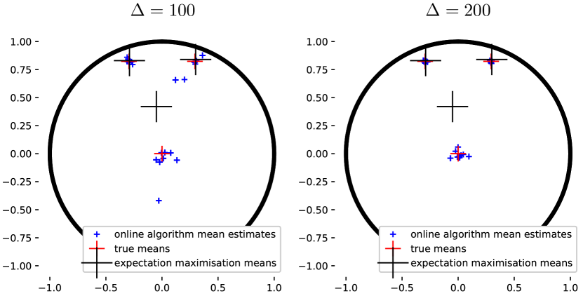
Figure 1: Mean estimates for multiple runs of the online algorithm for the example in the Poincaré disk for minibatch sizes of $\Delta=100$ and $\Delta=200$ compared with the EM algorithm estimates. As expected, the quality of the online algorithm estimates improves with minibatch size $\Delta$. We observe that for a relatively modest minibatch size of $\Delta=200$, the online algorithm is more accurate than the EM algorithm while being several orders of magnitude faster.

5 Conclusion

We have implemented an online algorithm for the learning of hidden Markov models on Hadamard spaces, i.e. an algorithm that uses a constant amount of memory instead of one that scales linearly with the amount of available data. We found that our algorithm outperforms a previous algorithm based on expectation-maximisation in all measures of accuracy when the right minibatch size is used. Furthermore, this improvement is achieved while running nearly 450 times faster and using 50 times less memory in the example considered.

Future work will consider strategies that would allow the removal of the $K$-means initialization step and automatically tune the minibatch size without the need for experimentation. Furthermore, significant challenges arise with increasing $N$, the number of states and hence dimension of the transition matrix. Here difficulties include identifying the correct number of clusters, preventing the algorithm from merging separate clusters (undercounting), and preventing the algorithm from double-counting clusters (overcounting) by assigning two means to the same cluster. These challenges have proven to be the main obstacles in increasing $N$. By contrast, increasing the dimension of the Hadamard space in which observations take place (e.g. the space of positive definite matrices) does not pose significant challenges and is straightforward using recent work on computing normalization factors of Riemannian Gaussian distributions [7, 16].

Appendix

The update rules and equations that describe our algorithm are summarized in Table 3. Here $f(x|y)$ denotes a conditional probability density function, $p_{i}(y)$ denotes the probability density function of the $i$th Gaussian distribution, and $k$ denotes the iteration index of the algorithm, and any quantity labelled by $k$ such as $p_{i}^{k}(y)$ denotes the $k$th best estimate of $p_{i}(y)$. Finally, $\Delta$ is the size of the subset of data (the so-called “minibatch”) that is loaded at any given time.

Table 3: Conditional probabilities and update rules

Symbol	Definition	Calculation
$\alpha_{t}(i)$	$f(y_{1},\dots,y_{t},s_{t}=i|\lambda^{(t-1)})$	$\alpha_{t}(j)=\sum_{i=1}^{N}\alpha_{t-1}(i)A_{ij}^{(t-1)}p_{j}^{(t-1)}(y_{t}),$ $\alpha_{1}(i)=\pi_{i}(i)p_{i}^{(1)}(y_{1})$
$\beta_{t|k}(i)$	$f(y_{t+1},\dots,y_{k}|s_{t}=i,\lambda^{(k-1)})$	$\beta_{k|k+\Delta}=A^{(k-1)}P^{(k-1)}(k+1)\dots A^{(k-1)}P^{(k-1)}(k+\Delta)\mathbf{1}$
$\gamma_{t|k}(i)$	$f(s_{t}=i|y_{1},\dots,y_{k},\lambda^{(k-1)})$	$\gamma_{t|k}(i)=\alpha_{t}(i)\beta_{t|k}(i)/\sum_{j=1}^{N}\alpha_{t}(j)\beta_{t|k}(j)$
$\zeta_{t|k}(i,j)$	$f(s_{t}=i,s_{t+1}=j|$ $y_{1},\dots,y_{k},\lambda^{(k-1)})$	$\frac{\alpha_{t}(i)A_{ij}^{(t-1)}\beta_{t+1|k}(j)p_{j}^{(t-1)}(y_{t+1})}{\sum_{i}\sum_{j}\alpha_{t}(i)A_{ij}^{(t-1)}\beta_{t+1|k}(j)p_{j}^{(t-1)}(y_{t+1})}$
$\mu_{j}^{i}(k)$	Intermediate calculation	$\sum_{t=1}^{k+1}\zeta_{t|k+1}(i,j)/(A^{(k+1)}_{ij})^{2}$
$g_{j}^{i}(k+1)$	Intermediate calculation	$\zeta_{k+1|k+1}(i,j)/A_{ij}^{(k+1)}$
$c_{i}(k+1)$	Means updates	$c_{i}(k)\#_{\tau}y_{k+1},\qquad\tau=\gamma_{k+1|k+1}(i)/\sum_{t=1}^{k+1}\gamma_{t|k+1}(i)$
$\delta_{i}^{(k+1)}$	$\delta$ update	$\delta_{i}^{(k)}+\frac{1}{\sqrt{k}}\gamma_{k+1|k+1}(i)\left(d^{2}\left(y_{k+1},c_{i}^{(k)}\right)-\delta_{i}^{(k)}\right)$
$A^{(k+1)}$	Transition matrix update	$A_{ij}^{(k)}+\frac{1}{\mu_{j}^{(i)}}\left(g_{j}^{(i)}-\frac{\sum_{h=1}^{N}g_{h}^{(i)}/\mu_{h}^{(i)}}{\sum_{h=1}^{N}1/\mu_{h}^{(i)}}\right)$

References

- [1] Arsigny, V., Fillard, P., Pennec, X., Ayache, N.: Log-Euclidean metrics for fast and simple calculus on diffusion tensors. Magnetic Resonance in Medicine 56(2), 411–421 (2006). https://doi.org/10.1002/mrm.20965
- [2] Barachant, A., Bonnet, S., Congedo, M., Jutten, C.: Multiclass brain–computer interface classification by Riemannian geometry. IEEE Transactions on Biomedical Engineering 59(4), 920–928 (2012)
- [3] Bini, D.A., Iannazzo, B.: Computing the Karcher mean of symmetric positive definite matrices. Linear Algebra and its Applications 438(4), 1700–1710 (2013). https://doi.org/10.1016/j.laa.2011.08.052
- [4] Cappé, O., Moulines, E., Rydén, T.: Inference in hidden Markov models. Springer Science & Business Media (2006)
- [5] Devijver, P.A.: Baum’s forward-backward algorithm revisited. Pattern Recognition Letters 3(6), 369–373 (1985)
- [6] Durbin, R., Eddy, S.R., Krogh, A., Mitchison, G.: Biological sequence analysis: probabilistic models of proteins and nucleic acids. Cambridge university press (1998)
- [7] Heuveline, S., Said, S., Mostajeran, C.: Gaussian distributions on Riemannian symmetric spaces in the large N limit. In: Nielsen, F., Barbaresco, F. (eds.) Geometric Science of Information. pp. 20–28. Springer International Publishing, Cham (2021)
- [8] Jeuris, B., Vandebril, R.: The Kähler mean of block-Toeplitz matrices with Toeplitz structured blocks. SIAM Journal on Matrix Analysis and Applications 37(3), 1151–1175 (2016). https://doi.org/10.1137/15M102112X
- [9] Krishnamurthy, V., Moore, J.B.: On-line estimation of hidden Markov model parameters based on the Kullback-Leibler information measure. IEEE Transactions on Signal Processing 41(8), 2557–2573 (1993). https://doi.org/10.1109/78.229888
- [10] Lang, S.: Fundamentals of differential geometry, vol. 191. Springer Science & Business Media (2012)
- [11] Li, S.Z.: Markov random field modeling in image analysis. Springer Science & Business Media (2009)
- [12] Pennec, X., Fillard, P., Ayache, N.: A Riemannian framework for tensor computing. International Journal of Computer Vision 66(1), 41–66 (Jan 2006). https://doi.org/10.1007/s11263-005-3222-z
- [13] Rabiner, L.R.: A tutorial on hidden Markov models and selected applications in speech recognition. Proceedings of the IEEE 77(2), 257–286 (1989). https://doi.org/10.1109/5.18626
- [14] Said, S., Bombrun, L., Berthoumieu, Y., Manton, J.H.: Riemannian Gaussian distributions on the space of symmetric positive definite matrices. IEEE Transactions on Information Theory 63(4), 2153–2170 (2017)
- [15] Said, S., Le Bihan, N., Manton, J.: Hidden Markov chains and fields with observations in Riemannian manifolds. IFAC-PapersOnLine 54(9), 719–724 (2021). https://doi.org/10.1016/j.ifacol.2021.06.135
- [16] Santilli, L., Tierz, M.: Riemannian Gaussian distributions, random matrix ensembles and diffusion kernels. Nuclear Physics B 973, 115582 (2021)