Variable Importance Scores

Abstract

Scoring of variables for importance in predicting a response is an ill-defined concept. Several methods have been proposed but little is known of their performance. This paper fills the gap with a comparative evaluation of eleven methods and an updated one based on the GUIDE algorithm. For data without missing values, eight of the methods are shown to be biased in that they give higher or lower scores to different types of variables, even when all are independent of the response. Of the remaining four methods, only two are applicable to data with missing values, with GUIDE the only unbiased one. GUIDE achieves unbiasedness by using a self-calibrating step that is applicable to other methods for score de-biasing. GUIDE also yields a threshold for distinguishing important from unimportant variables at 95 and 99 percent confidence levels; the technique is applicable to other methods as well. Finally, the paper studies the relationship of the scores to predictive power in three data sets. It is found that the scores of many methods are more consistent with marginal predictive power than conditional predictive power.

Keywords: Missing values, Prediction power, Recursive partitioning, Selection bias

1 Introduction

The question of how to quantify the relative importance of variables has intrigued researchers for years. While it was largely of academic interest early on, the question has taken on greater urgency in the last two decades, due to the increasing frequency of large data sets and the popularity of “black box” machine learning methods for which scoring the importance of variables may be the only means of interpretation; see Bring (1994), Bi (2012) and Wei et al. (2015) for excellent surveys. A prime black-box example is random forest (RF, Breiman (2001)), which consists of hundreds of unpruned regression trees. Its permutation-based scheme to produce importance scores has been copied by many methods.

Some researchers have observed that the orderings of RF scores do not always agree with those based on traditional methods. Bureau et al. (2005) used RF to identify single-nucleotide polymorphisms (SNPs) predictive of disease and found that while SNPs that are highly associated with disease, as measured by Fisher’s exact test, tend to have high RF scores, the two orderings do not match. Díaz-Uriarte and Alvarez de Andrés (2006) selected genes in microarray data by iteratively removing 20% of the genes with the lowest RF scores at each step. They found that this yielded a smaller set of genes than linear discriminant analysis, nearest neighbor and support vector machine methods, and that the RF results were more variable.

Table 1: Variables in COVID data

died	Died while hospitalized (0=no, 1=yes)
agecat	Age group (0=18–50, 1=50–59, 2=60–69, 3=70–79, 4=80–90 years)
race	White; Black or African American; Asian; Native Hawaiian or other Pacific Islander; American Indian or Alaska Native; Unknown
sex	Gender (male/female)
aids	AIDS/HIV (0=no, 1=yes)
cancer	Any malignancy, including lymphoma and leukemia, except malignant neoplasm of skin (0=no, 1=yes)
cerebro	Cerebrovascular disease (0=no, 1=yes)
charlson	Charlson comorbidity index (0–20)
CHF	Congestive heart failure (0=no, 1=yes)
CPD	Chronic pulmonary disease (0=no, 1=yes)
dementia	Dementia (0=no, 1=yes)
diabetes	Diabetes mellitus (0=no, 1=yes)
hemipara	Hemiplegia or paraplegia (0=no, 1=yes)
metastatic	Metastatic solid tumor (0=no, 1=yes)
MI	Myocardial infarction (0=no, 1=yes)
mildliver	Mild liver disease (0=no, 1=yes)
modsevliv	Moderate/severe liver disease (0=no, 1=yes)
PUD	Peptic ulcer disease (0=no, 1=yes)
PVD	Peripheral vascular disease (0=no, 1=yes)
RD	Rheumatic disease (0=no, 1=yes)
renal	Renal disease (0=no, 1=yes)

The differences in orderings may be demonstrated on a data set from Harrison et al. (2020) of 31,461 patients aged 18–90 years diagnosed with the COVID-19 disease between January 20 and May 26, 2020, in the United States. Table 1 lists the 21 variables, which consist of death during hospitalization, age group, sex, race, 16 comorbidities, and Charlson comorbidity index (a risk score computed from the comorbidities). The authors estimated mortality risk by fitting a multiple linear logistic regression model, without Charlson index, to each age group. They found 10 variables statistically significant at the 0.05 level (without multiplicity adjustment), namely, race, sex, and history of myocardial infarction (MI), congestive heart failure (CHF), dementia, chronic pulmonary disease (CPD), mild liver disease (mildliver), moderate/severe liver disease (modsevliv), renal disease (renal), and metastatic solid tumor (metastatic).

Figure 1 shows the importance scores of the top 10 variables obtained from 12 methods discussed below. There is substantial variation in the orderings, although agecat, charlson, and renal are ranked in the top 3 by 7 of the 12 methods. Of the variables that Harrison et al. (2020) found statistically significant, CPD is not ranked in the top 10 by any method, and mildliver and metastatic are ranked in the top 10 only twice and once, respectively. On the other hand, the non-significant variables cancer, cerebro, diabetes, hemipara, and PVD are ranked in the top 10 by 5, 10, 7, 3, and 9 methods, respectively. Statistical significance is clearly not necessarily consistent with the importance scores.

Figure 1: Top 10 variables for COVID data; scores of LASSO, RANGER, RF, RFSRC, and RLT are averaged over 100 runs with different random seeds

What is one to do in the face of such disparate results? One solution is to average the ranks across the methods, but this assumes that the methods are equally good. Strobl et al. (2007), Sandri and Zuccolotto (2008), and others have shown that the scores from RF are unreliable because they are biased towards certain variable types. A method is said to be “unbiased” if all predictor variables have the same mean importance score when they are independent of the response variable. One goal of this paper is to find out if other methods are biased.

Given a data set, bias may be uncovered by estimating the mean scores over random permutations of the response variable, keeping the values of the predictor variables fixed. Let $\mathtt{VI}_{j}(X)$ ($j=1,2,\ldots,J$) denote the importance score of variable $X$ in the $j$th permutation. Figure 2 plots the values of $\overline{\mathtt{VI}}(X)=J^{-1}\sum_{j}\mathtt{VI}_{j}(X)$ in increasing order and their 2-standard error bars, for $J=1000$. An unbiased method should have all its error bars overlapping. The plots show that only CFOREST2, GUIDE, and RANGER have this property.

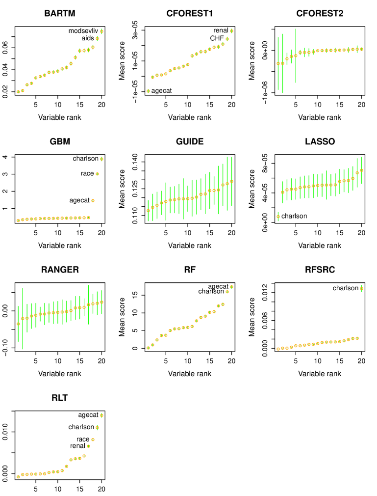
Figure 2: Mean importance scores $\overline{\mathtt{VI}}$ (orange) and 2-SE bars (green) from 1000 random permutations of the dependent variable for COVID data. Variables ordered by increasing mean scores. CTREE and RPART are not included because they returned trees with no splits (and hence no importance scores) for all permutations.

Another interesting problem is to identify variables that are truly important. There few attempts at answering this question, despite its being central to variable selection—an important step if the total number of variables exceeds the sample size. Although it may be expected that all important variables should be included, Loh (2012) showed that under certain conditions, omitting the less important ones can yield a model with higher prediction accuracy.

The remainder of this article is organized as follows. Section 2 describes the GUIDE method of calculating importance scores. Section 3 reviews the other 11 methods. Section 4 presents the results of simulations to identify the biased methods and show their effects on the scores. Section 5 examines the extent to which the scores of each method are consistent with two measures of predictive power of the variables. Section 6 describes a general procedure for producing a threshold score such that, with high probability, variables with scores less than the threshold are independent of the response. Section 7 shows how the GUIDE method applies to data with missing values. Section 8 concludes the article with some remarks.

2 GUIDE

The GUIDE algorithm for constructing regression and classification trees is described in Loh (2002) and Loh (2009), respectively. It differs from CART (Breiman et al., 1984) in every respect except tree pruning, where both employ the same cost-complexity cross-validation technique. CART uses greedy search to select the split that most decreases node impurity but GUIDE uses chi-squared tests to first select a split variable and then searches for the best split based on it that most decreases node impurity. This approach started in Loh and Vanichsetakul (1988) and evolved principally through Chaudhuri et al. (1994), Loh and Shih (1997), and Loh (2002, 2009). Besides reducing computation, it lets GUIDE avoid biases in variable selection inherent among greedy search methods. Another major difference between GUIDE and CART is how each deals with missing values in predictor variables. Kim and Loh (2001) showed that CART’s solution through surrogate splits is another source of selection bias.

An initial importance scoring method based on GUIDE was proposed in Loh (2012). Though not designed to be unbiased, it turned out to be approximately unbiased unless there is a mix of ordinal and categorical variables. We present here an improved version for regression that ensures unbiasedness. As in the previous method, it uses a weighted sum of chi-squared statistics obtained from a shallow (four-level) unpruned tree, but it adds conditional tests for interaction and a permutation-based step for bias adjustment. Given a node $t$, let $n_{t}$ denote the number of observations in $t$.

1. Fit a constant to the data in $t$ and compute the residuals.

2. Define a class variable $Z$ such that $Z=1$ if the observation has a positive residual and $Z=2$ otherwise.

3. 1. If $X_{k}$ is an ordinal variable, transform it to a categorical variable $X_{k}^{\prime}$ with $m$ roughly equal-sized categories, where $m=3$ if $n_{t}<60$ and $m=4$ otherwise.

   2. If $X_{k}$ is a categorical variable, define $X_{k}^{\prime}=X_{k}$.

4. If $X_{k}$ has missing values, add an extra category to $X_{k}^{\prime}$ to hold the missing values.

5. For $k=1,2,\ldots,K$, where $K$ is the number of variables, perform a contingency table chi-squared test of $X_{k}^{\prime}$ versus $Z$ and denote its p-value by $p_{1}(k,t)$.

6. If $\min_{k}p_{1}(k,t)\geq 0.10/K$ (first Bonferroni correction), carry out the following interaction tests.

   1. Transform each ordinal $X_{k}$ to a 3-level categorical variable $X_{k}^{\prime}$. If $X_{k}$ has no missing values, $X_{k}^{\prime}$ is $X_{k}$ discretized at the 33rd and 67th sample quantiles. If $X_{k}$ has missing values, $X_{k}^{\prime}$ is $X_{k}$ discretized at the sample median with missing values forming the third category. If $X_{k}$ is a categorical variable, let $X_{k}^{\prime}=X_{k}$.

   2. For every pair $(X^{\prime}_{j},X^{\prime}_{k})$ with $j<k$, perform a chi-squared test with the $Z$ values as rows and the $(X^{\prime}_{j},X^{\prime}_{k})$ values as columns and let $p_{2}(j,k,t)$ denote its p-value.

   3. Let $(X_{j^{\prime}}^{\prime},X_{k^{\prime}}^{\prime})$ be the pair of variables with the smallest value of $p_{2}(j,k,t)$. If $p_{2}(j^{\prime},k^{\prime},t)<0.20\{K(K-1)\}^{-1}$ (second Bonferroni correction), redefine $p_{1}(j^{\prime},t)=p_{1}(k^{\prime},t)=p_{2}(j^{\prime},k^{\prime},t)$.

7. Let $k^{*}$ be the smallest value of $k$ such that $p_{1}(k^{*},t)=\min_{k}p_{1}(k,t)$. Find the split on $X_{k^{*}}$ yielding the largest decrease in node impurity (i.e., sum of squared residuals).

After a tree is grown with four levels of splits, the importance score of $X_{k}$ is computed as

$$v(X_{k})=\sum_{t}\sqrt{n_{t}}\,\chi^{2}_{1}(k,t)$$ (1)

where the sum is over the intermediate nodes and $\chi^{2}_{1}(k,t)$ denotes the $(1-p_{1}(k,t))$-quantile of the chi-squared distribution with 1 degree of freedom. The factor $\sqrt{n_{t}}$ in (1) first appeared in Loh (2012) but was changed to $n_{t}$ in Loh et al. (2015); we revert it back to $\sqrt{n_{t}}$ to prevent the root node from dominating the scores.

The values of $v(X_{k})$ are slightly biased due partly to differences between ordinal and categorical variables and partly to the above step 6. To remove the bias, we adjust the scores by their means computed under the hypothesis that the response variable ($Y$) is independent of the $X$ variables. Specifically, the $Y$ values are randomly permuted $B$ times (the default is $B=300$) with the $X$ values fixed, and a tree with four levels of splits is constructed for each permuted data set. Let $v^{*}_{b}(X_{k})$ be the value of (1) in permutation $b=1,2,\ldots,B$, and define $\bar{v}(X_{k})=B^{-1}\sum_{b}v^{*}_{b}(X_{k})$. The GUIDE bias-adjusted variable importance score of $X_{k}$ is

$$\mathtt{VI}(X_{k})=v(X_{k})/\bar{v}(X_{k}).$$ (2)

3 Other methods

We briefly review the other methods here.

RPART.

This is an R version of CART (Therneau and Atkinson, 2019a). Let $s=\{X_{i}\in A\}$ denote a split of node $t$ for some variable $X_{i}$ and set $A$, and let $t_{L}$ and $t_{R}$ denote its left and right child nodes. Given a node impurity function $i(t)$ at $t$, let $\Delta(s,t)=i(t)-i(t_{L})-i(t_{R})$ be a measure of the goodness of the split. For regression trees, $i(t)=\sum_{i\in t}(y_{i}-\bar{y}_{t})^{2}$, where $\bar{y}_{t}$ is the sample mean at $t$. CART partitions the data with the split $s(t)$ that maximizes $\Delta(s,t)$. To evaluate the importance of the variables as well as to deal with missing values, CART finds, for each $X_{j}$ ($j\neq i$), the surrogate split $\tilde{s}_{j}(t)$ that best predicts $s(t)$. The importance score of $X_{j}$ is $\sum_{t}\Delta(\tilde{s}_{j}(t),t)$, where the sum is over the intermediate nodes of the pruned tree (Breiman et al., 1984, p. 141).

RPART measures importance differently from CART (Therneau and Atkinson, 2019b). Given a split $s(t)$ and a surrogate $\tilde{s}(t)$, let $k(s(t),\tilde{s}(t))$ be the total number of observations in $t_{L}$ and $t_{R}$ correctly sent by $\tilde{s}(t)$. Let $n_{L}$ and $n_{R}$ denote the number of observations in $t_{L}$ and $t_{R}$, respectively. The “adjusted agreement” between $s$ and $\tilde{s}$ is $a(s,\tilde{s})=\{k(s,\tilde{s})-\max(n_{L},n_{R})\}/\min(n_{L},n_{R})$. Call $X_{i}$ a “primary” variable if it is in $s$ and a “surrogate” variable if it is in $\tilde{s}$. Let $P(i)$ and $S(i)$ denote the sets of intermediate nodes where $X_{i}$ is the primary and surrogate variable, respectively. RPART defines $\mathtt{VI}(X_{i})=\sum_{t\in P(i)}\Delta(s(t),t)+\sum_{t\in S(i)}a(s(t),\tilde{s}(t))\Delta(\tilde{s}(t),t)$ as the importance score of $X_{i}$. As shown below, this method yields biased scores, because maximizing the decrease in node impurity induces a bias towards selecting variables that allow more splits (White and Liu, 1994; Loh and Shih, 1997) and the surrogate split method itself induces a bias when there are missing values (Kim and Loh, 2001).

GBM.

This is gradient boosting machine (Friedman, 2001). It uses functional gradient descent to build an ensemble of short CART trees. For a single tree, the importance score of a variable is the square root of the total decrease in node impurity (squared error in the case of regression) over the nodes where the variable appears in the split. For an ensemble, it is the root mean squared importance score of the variable over the trees (Friedman, 2001, p. 1217). We use the R function gbm (Greenwell et al., 2019) to construct the GBM models and the varImp function in the caret package (Kuhn, 2020) to calculate the importance scores.

RF.

This is the R implementation of random forest (Liaw and Wiener, 2002). It has two measures for computing importance scores. The first is the “decrease in accuracy” of the forest in predicting the “out-of-bag” (OOB) data before and after random permutation of the predictor variable, where the OOB data are the observations not in the bootstrap sample. The second uses the “decrease in node impurity,” which is the average of the total decrease in node impurity of the trees. Partly due to CART’s split selection bias, the decrease in node impurity measure is known to be unreliable (Strobl et al., 2007; Sandri and Zuccolotto, 2008). The results reported here use the “decrease in accuracy” measure.

RANGER.

Sandri and Zuccolotto (2008) used pseudovariables to correct the bias in RF’s “decrease in node impurity” method. (Pseudovariables were employed earlier by Wu et al. (2007).) Given $K$ predictor variables $\mathbf{X}=(X_{1},X_{2},\ldots,X_{K})$, another $K$ pseudovariables $\mathbf{Z}=(Z_{1},Z_{2},\ldots,Z_{K})$ are added where the rows of $\mathbf{Z}$ are random permutations of the rows of $\mathbf{X}$. The RF algorithm is applied to the $2K$ predictors and the importance score of $X_{i}$ is adjusted by subtracting the score of $Z_{i}$ for $i=1,2,\ldots,K$. This approach requires more computer memory and increases computation time (a forest has to be constructed for each generation of $\mathbf{Z}$). Nembrini et al. (2018) proposed using only a single generation of $\mathbf{Z}$ and storing only the permutation indices rather than the values of $\mathbf{Z}$. Their method is implemented in the ranger R package (Wright and Ziegler, 2017). Although storing only the permutation indices saves computer memory, the use of a single permutation adds another level of randomness to the already random results of RF. In serious applications, there are no savings in computation time because RANGER must be applied many times to stabilize the average importance scores. In the real data examples here, the RANGER scores are averages over 100 replications.

RFSRC.

This is another ensemble method similar to RF (Ishwaran, 2007; Ishwaran et al., 2008). The importance of a variable $X$ is measured by the difference between the prediction error of the OOB sample before and after $X$ is “noised up”. “Noising up” here means that if an OOB observation encounters a split on $X$ at a node $t$, it is randomly sent to the left or right branch, with equal probability, at $t$ and all its descendent nodes. Missing values in a predictor variable are imputed nodewise, by replacing each missing value with a randomly selected non-missing value in the node. The results for RFSRC here are obtained with the randomForestSRC R package (Ishwaran and Kogalur, 2007).

RLT.

This method may be thought of as “RF-on-RF.” Called “reinforcement learning trees” (Zhu et al., 2015), it constructs an ensemble of trees from bootstrap samples, but uses the RF permutation-based importance scoring method to select the most important variable to split each node in each tree. After the ensemble is constructed, the final importance scores are obtained using the RF permutation scheme. The results here are produced by the RLT package (Zhu, 2018).

CTREE.

This is the “conditional inference tree” algorithm of Hothorn et al. (2006). It follows the GUIDE approach of using significance tests to select a variable to split each node of a tree. Unlike GUIDE, however, CTREE uses linear statistics based on a permutation test framework and, instead of pruning, it uses Bonferroni-type p-value thresholds to determine tree size. Further, the significance tests employ only observations with non-missing values in the $X$ variable being evaluated. Observations with missing values are passed through each split by means of surrogate splits as in CART. Importance scores are obtained as in RFSRC, except that an OOB observation missing the split value at a node is randomly sent to the left or right child node with probabilities proportional to the samples sizes of the non-missing observations in the child nodes.

CFOREST.

This is an ensemble of CTREE trees from the partykit R package. Instead of bootstrap samples, it takes random subsamples (without replacement) of about two-thirds of the data to construct each tree. Strobl et al. (2007) showed that this removes a bias in RF that gives higher scores to categorical variables with large numbers of categories. This is the default option in partykit, which we denote by CFOREST1. Another option, which we denote by CFOREST2, is conditional permutation of the variables, which Strobl et al. (2008) proposed for reducing the bias in RF towards correlated variables.

LASSO.

This is linear regression with the lasso penalty. The importance score of an ordinal variable is the absolute value of its coefficient in the fitted model and that of a categorical variable is the average of the absolute values of the coefficients of its dummy variables. All variables (including dummy variables) are standardized to have mean 0 and variance 1 prior to model fitting. We use the R implementation in the glmnet package (Friedman et al., 2010).

BARTM.

This is bartMachine (Bleich et al., 2014), a Bayesian method of constructing a forest of regression trees using the BART (Chipman et al., 2010) method. The underlying model is that the response variable is a sum of regression tree models plus homoscedastic Gaussian noise. Prior distributions must be specified for all unknown parameters, including the set of tree structures, terminal node parameters, and the Gaussian noise variance. According to Bleich et al. (2014), the importance of a variable is given by the relative frequency that it appears in the splits in the trees. The results here are obtained from the R package bartMachine with default parameters.

4 Simulation experiments

We performed 6 simulation experiments (E0–E5) involving 11 predictor variables ($B_{1}$, $B_{2}$, $C_{1}$, $C_{2}$, $N_{1}$, $N_{2}$, $N_{3}$, $N_{4}$, $S_{1}$, $S_{2}$, $S_{3}$) to compare the performance of the methods. Variable sets $\{B_{1}\}$, $\{C_{1}\}$, $\{B_{2},C_{2}\}$, $\{N_{1},N_{2},N_{3},N_{4}\}$, and $\{S_{1},S_{2},S_{3}\}$ are mutually independent. Variable $B_{1}$ is Bernoulli with $P(B_{1}=1)=0.50$, and $C_{1}$, $C_{2}$ are independent categorical variables taking values $1,2,\ldots,10$ with equal probability 0.10. Variable $B_{2}=I(C_{2}\leq 5)$ is a binary variable derived from $C_{2}$. Variable $N_{1}$ is independent standard normal except in model E2 (see below). The triple $(N_{2},N_{3},N_{4})$ is multivariate normal with zero mean, unit variance, and constant correlation 0.90. The triple $(S_{1},S_{2},S_{3})$ is obtained by setting $S_{1}=\min(U_{1},U_{2})$, $S_{2}=|U_{1}-U_{2}|$, and $S_{3}=1-\max(U_{1},U_{2})$, where $U_{1}$ and $U_{2}$ are independent and uniformly distributed variables on the unit interval, so that $S_{1}+S_{2}+S_{3}=1$ and $\mbox{cor}(S_{i},S_{j})=-0.50$ ($i\neq j$). Their purpose is to see if there any effects of linear dependence on the importance scores.

Table 2 shows the models used to generate the dependent variable $Y=\mu(X)+\epsilon$, where $\mu(X)$ is a function of the predictor variables and $\epsilon$ an independent standard normal variable. Null model E0, where $Y$ is independent of the $X$ variables, tests for bias. The other models, which have one or two important variables, show the effects of bias on the scores. For each model, the scores are obtained from 1000 simulation trials, with random samples of 400 observations in each trial.

Figure 3 shows the average scores and their 2-SE (simulation standard error) bars for model E0. Because the 2-SE bars should overlap if there is no selection bias, we see that only CFOREST2, CTREE, GUIDE, and RANGER are unbiased, with RANGER and, to a lesser degree, CFOREST2 exhibiting variance heterogeneity. BARTM, CFOREST1 and RF are biased towards correlated variables $N_{2}$, $N_{3}$ and $N_{4}$. GBM, RLT and RPART are biased towards categorical variables $C_{1}$ and $C_{2}$. RFSRC is biased against all categorical variables. LASSO is biased in favor of $B_{1}$ but against $B_{2}$.

Table 2: Simulation models $Y=\mu(X)+\epsilon$, with $\epsilon$ independent standard normal

E0	$\mu(X)=0$
E1	$\mu(X)=0.2N_{2}$
E2	$\mu(X)=0.1(N_{1}+N_{2})$
E3	$\mu(X)=0.2B_{1}$
E4	$\mu(X)=0.2B_{2}=0.2I(C_{2}\leq 5)$
E5	$\mu(X)=0.5\{I(B_{1}=0,C_{1}\leq 5)+I(B_{1}=1,C_{1}>5)\}$

Figure 3: Average importance scores with 2-SE error bars for model E0, where predictor variables are independent of $Y$.

Figures 4–8 show boxplots of the 1000 simulated scores for models E1–E5. Boxplots of variables that affect $Y$ are drawn in red. We can draw the following conclusions.

E1.

The model is $\mu(X)=0.2N_{2}$, but the response is also associated with $N_{3}$ and $N_{4}$ through their correlation with $N_{2}$. Figure 4 shows that all but one method give their highest median scores to these three predictors. The exception is GBM—its strong bias towards variables $C_{1}$ and $C_{2}$ makes them likely to be incorrectly scored higher than $N_{2}$, $N_{3}$ and $N_{4}$.

E2.

The model is $\mu(X)=0.1(N_{1}+N_{2})$, where $N_{1}$ is independent of $N_{2}$ but the latter is highly correlated with $N_{3}$ and $N_{4}$. We expect their scores to be larger than those of the other variables, with $N_{1}$ and $N_{2}$ being roughly equal and $N_{3}$ and $N_{4}$ close behind. Figure 5 shows this to be true of all methods except GBM, RF, RLT, and RPART. For RF and RPART, the presence of $N_{3}$ and $N_{4}$ raises the median score of $N_{2}$ above that of $N_{1}$. GBM again tends to incorrectly score $C_{1}$ and $C_{2}$ highest. RLT also frequently incorrectly scores these two categorical variables higher than $N_{2}$, $N_{3}$ and $N_{4}$.

E3.

The model is $\mu(X)=0.2B_{1}$, with $B_{1}$ independent of the other predictors. All except GBM, LASSO, RF, RFSRC, RLT, and RPART are more likely to correctly score $B_{1}$ highest. GBM, RLT and RPART fail to do this due to bias towards $C_{1}$ and $C_{2}$. RF fails due to the high correlation of $N_{2}$, $N_{3}$ and $N_{4}$. CTREE and LASSO yield median scores of 0 for all predictors, including $B_{1}$.

E4.

The model is $\mu(X)=0.2B_{2}$ but because $B_{2}=I(C_{2}\leq 5)$, the two should have the highest median importance scores. Only GUIDE, RANGER and possibly CFOREST2 have this property. BARTM and CFOREST1 give the highest median score to $B_{2}$ but midling median scores to $C_{2}$. Conversely, due to their bias towards categorical variables, GBM and RLT give the highest median score to $C_{2}$ but midling median scores to $B_{2}$. As in model E3, CTREE and LASSO cannot reliably identify $B_{2}$ or $C_{2}$ as important because both methods yield 0 median scores for all predictors.

E5.

The model is $\mu(X)=0.5\{I(B_{1}=0,C_{1}\leq 5)+I(B_{1}=1,C_{1}>5)\}$, which has an interaction between $B_{1}$ and $C_{1}$. BARTM, CFOREST1, CFOREST2, GUIDE, and RANGER correctly give highest median scores to these two predictors. GBM and RPART give $B_{1}$ the lowest median score due to their bias against binary variables. RF incorrectly gives $B_{1}$ and $C_{1}$ low median scores due to its preference for correlated predictors. RFSRC incorrectly gives $B_{1}$ and $C_{1}$ low median scores due to its bias against binary and categorical predictors. RLT gives $C_{1}$ and $C_{2}$ the highest median scores due to its bias towards these two variables. CTREE and LASSO are again ineffective because both give zero median scores to all predictors.

Overall, CFOREST2, GUIDE, and RANGER are the only unbiased methods and consequently are among the most likely to correctly identify the important variables.

Figure 4: Boxplots of importance scores over 1000 trials for model E1, where $\mu(X)=0.2N_{2}$ and $N_{2},N_{3}$, $N_{4}$ are highly correlated. Variables associated with $Y$ are in red.

Figure 5: Boxplots of importance scores over 1000 trials for model E2 where $\mu(X)=0.1(N_{1}+N_{2})$ and $N_{2},N_{3},N_{4}$ are highly correlated. Variables with effect on $Y$ are in red.

Figure 6: Boxplots of importance scores over 1000 trials for model E3, where $\mu(X)=0.2B_{1}$. Variables with effect on $Y$ are in red.

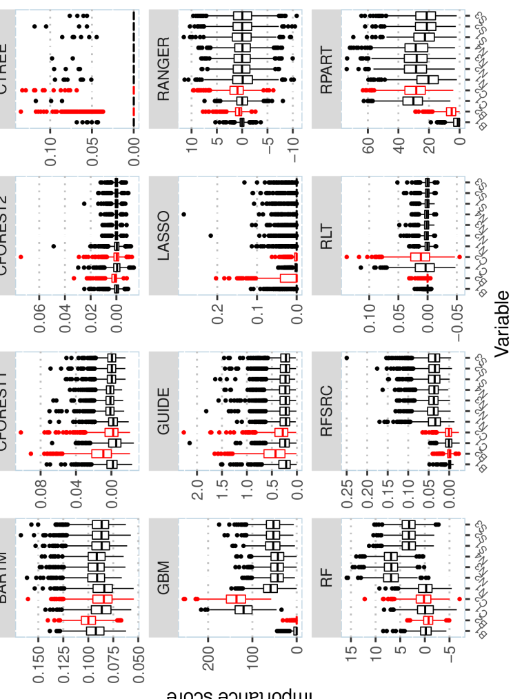
Figure 7: Boxplots of importance scores over 1000 trials for model E4, where $\mu(X)=0.2B_{2}$ and $B_{2}=I(C_{2}\leq 5)$. Variables with effect on $Y$ are in red.

Figure 8: Boxplots of importance scores over 1000 trials for model E5, where $\mu(X)=0.5\{I(B_{1}=0,C_{1}\leq 5)+I(B_{1}=1,C_{1}>5)\}$. Variables with effect on $Y$ are in red.

5 Predictive importance

“Predictive importance” may be interpreted as the effect of a variable on the prediction of a response, but it is not known which, if any, of the importance scoring methods directly measures the concept. BARTM scores variables by their frequencies of being chosen to split the nodes of the trees. GBM and RPART base their scores on decrease in impurity, and LASSO uses absolute values of regression coefficient estimates. CFOREST, CTREE, RANGER, RF, and RFSRC measure change in prediction accuracy after random permutation of the variables—an approach that Strobl et al. (2008) call “permutation importance.” GUIDE scores may be considered as measures of “associative importance,” being based on chi-squared tests of association with the response variable at the nodes of a tree.

To see how well the scores reflect predictive importance, we need a precise definition of the latter. Given predictor variables $X_{1},X_{2},\ldots,X_{K}$, consider the four models,

$$Y = \mu+\epsilon$$ (3)

$$Y = f_{j}(X_{j})+\epsilon$$ (4)

$$Y = g_{j}(X_{1},\ldots,X_{j-1},X_{j+1},\ldots,X_{K})+\epsilon$$ (5)

$$Y = h(X_{1},X_{2},\ldots,X_{K})+\epsilon$$ (6)

where $\mu$ is a constant, $f_{j}$, $g_{j}$, and $h$ are arbitrary functions of their arguments, and $\epsilon$ is an independent variable with zero mean and variance possibly depending on the values of the $X$ variables. Equation (3) states that $E(Y)$ is independent of the predictors, (4) states that it depends only on $X_{j}$, (5) states that it depends on all variables except $X_{j}$, and (6) allows dependence on all variables. Let $\hat{\mu}$, $\hat{f}_{j}$, $\hat{g}_{j}$, and $\hat{h}$ denote estimates of $\mu$, $f_{j}$, $g_{j}$, and $h$, respectively, obtained from a training sample and define

$$S_{0} = E(Y-\hat{\mu})^{2}$$

$$S_{j} = E(Y-\hat{f}_{j}(X_{j}))^{2}$$

$$S_{-j} = E(Y-\hat{g}_{j}(X_{1},\ldots,X_{j-1},X_{j+1},\ldots,X_{K}))^{2}$$

$$S = E(Y-\hat{h}(X_{1},\ldots,X_{K}))^{2}$$

where the expectations are computed with $\hat{\mu}$, $\hat{f}_{j}$, $\hat{g}_{j}$, and $\hat{h}$ fixed. We call $(S_{0}-S_{j})$ the marginal predictive value of $X_{j}$ because it is the difference in mean squared error between predicting $Y$ with and without $X_{j}$, ignoring the other predictors. We call $(S_{-j}-S)$ the conditional predictive value of $X_{j}$ because it is the difference in mean squared error between predicting $Y$ without and with $X_{j}$, with the other predictors included.

Correlations between the importance scores and marginal and conditional predictive values indicate how well the former reflects the latter. To compute the correlations for a given data set, we need first to estimate $\mu$, $f_{j}$, $g_{j}$, and $h$. Here we use the average of 5 ensemble methods, namely, CFOREST, GBM, GUIDE forest, RANGER, and RFSRC to obtain the estimates. This helps to ensure that no scoring method has an unfair advantage. We use leave-one-out cross-validation to estimate $S_{0}$, $S_{j}$, $S_{-j}$, and $S$. Specifically, given a data set $\{(y_{i},x_{i1},\ldots,x_{iK})\}$, $i=1,2,\ldots,n$, define the vectors and matrices

$$\mathbf{x}_{j} = (x_{1j},x_{2j},\ldots,x_{nj})^{\prime}$$

$$\mathbf{x}_{j}^{(-i)} = (x_{1j},x_{2j},\ldots,x_{i-1,j},x_{i+1,j},\ldots,x_{nj})^{\prime}$$

$$\mathbf{X} = (\mathbf{x}_{1},\mathbf{x}_{2},\ldots,\mathbf{x}_{K})$$

$$\mathbf{X}^{(-i)} = (\mathbf{x}_{1}^{(-i)},\mathbf{x}_{2}^{(-i)},\ldots,\mathbf{x}_{K}^{(-i)})$$

$$\mathbf{X}_{(-j)} = (\mathbf{x}_{1},\mathbf{x}_{2},\ldots,\mathbf{x}_{j-1},\mathbf{x}_{j+1},\ldots,\mathbf{x}_{K})$$

$$\mathbf{X}_{(-j)}^{(-i)} = (\mathbf{x}_{1}^{(-i)},\mathbf{x}_{2}^{(-i)},\ldots,\mathbf{x}_{j-1}^{(-i)},\mathbf{x}_{j+1}^{(-i)},\ldots,\mathbf{x}_{K}^{(-i)})$$

where $(\mathbf{x}_{j}^{(-i)},\mathbf{X}^{(-i)},\mathbf{X}_{(-j)}^{(-i)})$ are $(\mathbf{x}_{j},\mathbf{X},\mathbf{X}_{(-j)})$ without the $i$th row and $(\mathbf{X}_{(-j)},\mathbf{X}_{(-j)}^{(-i)})$ are $(\mathbf{X},\mathbf{X}^{(-i)})$ without the $j$th column. Let $(\hat{f}_{j}^{(-i)},\hat{g}_{j}^{(-i)},\hat{h}^{(-i)})$ denote the function estimates of $(f_{j},g_{j},h)$ based on $(\mathbf{x}_{j}^{(-i)},\mathbf{X}_{(-j)}^{(-i)},\mathbf{X}^{(-i)})$, respectively, using the average of the 5 ensemble methods. Let $\bar{y}=n^{-1}\sum_{k}y_{k}$, $\bar{y}^{(-i)}=(n-1)^{-1}\sum_{k\neq i}y_{k}$ and define the leave-one-out mean squared errors

$$\hat{S}_{0} = n^{-1}\sum_{i=1}^{n}(y_{i}-\bar{y}^{(-i)})^{2}$$

$$\hat{S}_{j} = n^{-1}\sum_{i=1}^{n}\{y_{i}-\hat{f}_{j}^{(-i)}(x_{ij})\}^{2}$$

$$\ \hat{S}_{-j} = n^{-1}\sum_{i=1}^{n}\{y_{i}-\hat{g}_{j}^{(-i)}(x_{i1},x_{i2},\ldots,x_{i,j-1},x_{i,j+1},\ldots,x_{iK})\}^{2}$$

$$\hat{S} = n^{-1}\sum_{i=1}^{n}\{y_{i}-\hat{h}^{(-i)}(x_{i1},x_{i2},\ldots,x_{iK})\}^{2}.$$

Denote the estimated marginal and conditional predictive values by $\mathtt{MPV}_{j}=\hat{S}_{0}-\hat{S}_{j}$ and $\mathtt{CPV}_{j}=\hat{S}_{-j}-\hat{S}$. We compute them for the following three real data sets.

Baseball.

The data give performance and salary information of 263 North American Major League Baseball players during the 1986 season (Denby, 1986). The response variable is log-salary and there are 22 predictor variables; see Hoaglin and Velleman (1995) and references therein for definitions of the variables. The plot on the left side of Figure 9 shows a rather weak correlation of 0.318 between $\mathtt{CPV}$ and $\mathtt{MPV}$. Variable Yrs (number of years in the major leagues) has high values of $\mathtt{MPV}$ and $\mathtt{CPV}$ but Batcr (number of times at bat during career) has a high value of $\mathtt{MPV}$ and a negative value of $\mathtt{CPV}$. This implies that Batcr is an excellent predictor if it is used alone, but its addition after the other variables are included does not increase accuracy.

Mpg.

This data set gives the characteristics, price, and dealer cost of 428 new model year 2004 cars and trucks (Johnson, 2004). We use 14 variables to predict city miles per gallon (mpg). The middle panel of Figure 9 shows that Hp (horsepower) has the highest values of $\mathtt{MPV}$ and $\mathtt{CPV}$. Variable Make (which has 38 categorical values) has the second highest $\mathtt{CPV}$ but its $\mathtt{MPV}$ is below average, indicating that its predictive power is mainly derived from interactions with other variables. The correlation between $\mathtt{CPV}$ and $\mathtt{MPV}$ is 0.378.

Solder.

Chambers and Hastie (1992) used the data from a circuit board soldering experiment to demonstrate Poisson regression in R. The data, named solder.balance in the rpart R package, give the number of solder skips in a 5-factor unreplicated $3\times 2\times 4\times 10\times 3$ factorial experiment. Because not all scoring methods are applicable to Poisson regression, we use least squares with dependent variable the square root of the number of solder skips. The right panel of Figure 9 shows that $\mathtt{CPV}$ and $\mathtt{MPV}$ are almost perfectly correlated. This is a consequence of the factorial design.

Figure 9: CPV versus MPV and their correlations for three data sets

Table 3: Correlations between importance scores VI and marginal and conditional predictive values MPV and CPV

	Baseball		Mpg		Solder
Method	MPV	CPV	MPV	CPV	MPV	CPV
BARTM	0.75	0.68	0.85	0.48	0.4	0.46
CFOREST1	0.87	0.1	0.82	0.28	1	1
CFOREST2	0.82	0.16	0.69	0.78	0.99	1
CTREE	0.4	0.07	0.65	0.54	0.99	1
GBM	0.8	0.14	0.62	0.88	0.99	0.98
GUIDE	0.99	0.3	0.94	0.24	0.9	0.92
LASSO	0.19	0.59	0.75	0.55	0.73	0.76
RANGER	0.97	0.18	0.96	0.33	1	1
RF	0.83	0.16	0.54	0.28	0.87	0.91
RFSRC	0.79	0.02	0.72	0.8	1	1
RLT	0.69	0	0.67	0.77	0.99	1
RPART	0.92	0.2	0.85	0.44	0.9	0.93

Table 3 gives the correlations between the importance scores VI and each of MPV and CPV for each method and Figure 10 shows them graphically. The results may be summarized as follows.

Baseball.

The importance scores are highly correlated with MPV for GUIDE and RANGER, but not for LASSO where there is barely any correlation. On the other hand, the scores are weakly correlated with CPV for all methods except BARTM and LASSO.

Mpg.

GUIDE and RANGER are again the two methods with importance scores most highly correlated with MPV; the correlations for the other methods range from 0.54 for RF to 0.85 for BARTM and RPART. For CPV, GBM has the highest correlation of 0.88, followed by RFSRC (0.0.80) and CFOREST2 (0.78).

Solder.

Owing to the almost perfect correlation between MPV and CPV, their correlations with the importance scores are almost the same. BARTM and LASSO are the only two methods with correlations substantially below 0.90, indicating that they are measuring something besides MPV and CPV.

Across the three data sets, the importance scores of all methods, except for BARTM and LASSO, are consistent with MPV, with GUIDE, RANGER and RPART showing the highest consistency. Consistency with CPV is weaker and more variable between data sets.

Figure 10: Plots of (cor(VI, CPV), cor(VI, MPV)) for three data sets; B = BARTM, Cf1 = CFOREST1, Cf2 = CFOREST2, Ct = CTREE, Gb = GBM, Gu = GUIDE, L = LASSO, Ra = RANGER, Rf = RF, Rfs = RFSRC, Rl = RLT, Rp = RPART

6 Thresholding

It is useful to have a score threshold to identify the variables that are independent of the response. This is particularly desirable if the number of variables is large. Of the 12 scoring methods, only BARTM and GUIDE currently provide thresholds. We call a variable “unimportant” if it is independent of the response variable and “important” otherwise. Under the null hypothesis $H_{0}$ that all variables are unimportant, we define a “Type I error” as that of declaring at least one to be important. To control the probability of this error at significance level $\alpha$, Bleich et al. (2014) randomly permute the $Y$ values several times, keeping the $X$ values fixed. They construct a BARTM forest to each set of permuted data, derive several candidate thresholds from the permutation distributions of the variable selection frequencies, and use cross-validation to choose among them.

GUIDE similarly permutes the $Y$ values, keeping the $X$ values fixed. For $j=1,2,\ldots,300$, let $u_{j}=\max_{i}\mathtt{VI}(X_{i})$ denote the maximum value of the GUIDE importance scores for the $j$th permuted data set and let $u^{*}(\alpha)$ be the $(1-\alpha)$-quantile of the distribution of $\{u_{1},u_{2},\ldots,u_{300}\}$. Under $H_{0}$, the probability that one or more importance scores exceeds the value of $u^{*}(\alpha)$ is approximately $\alpha$.

Bias adjustment of the importance scores defined in equation (2) requires one level of permutation. Calculation of $u^{*}(\alpha)$ requires a second level of permutation. To skip the second level, GUIDE uses the following approximation. In the permutations for bias adjustment, let $v_{b}=\max_{i}v^{*}_{b}(X_{i})$, $b=1,2,\ldots,B$, denote the maximum unadjusted score, where $v^{*}_{b}(X_{i})$ is defined above equation (2). Let $v^{*}(\alpha)$ denote the $(1-\alpha)$-quantile of $\{v_{1},v_{2},\ldots,v_{B}\}$. Let $s(X_{i})$ be the unadjusted score for the unpermuted (real) data defined in (1). Finally, let $m$ denote the number of values of $s(X_{i})$ greater than $v^{*}(\alpha)$. We declare the variables with the top $m$ values of the bias-adjusted scores $\mathtt{VI}(X_{i})$ to be important. Let $\tilde{v}(\alpha)$ denote the average of the $m$th and $(m+1)$th largest values of $\mathtt{VI}(X_{i})$. The GUIDE normalized importance scores are $\mathtt{VI}(X_{i})/\tilde{v}(\alpha)$, so that variables with normalized scores less than 1.0 are considered unimportant.

Table 4: Important variables (in alphabetical order for BARTM, in decreasing importance for GUIDE) for $\alpha=0.05$

Data	BARTM	GUIDE
COVID	diabetes, race=Black or African American, race=Unknown, race=White	renal, charlson, agecat, MI, CHF, dementia, PVD, cerebro, cancer, diabetes, race, CPD, sex, metastatic, hemipara, modsevliv, mildliver
Baseball	Hitcr, Rbcr, Runcr, Yrs	Batcr, Hitcr, Runcr, Rbcr, Wlkcr, Yrs, Hrcr, Hit86, Rb86, Bat86, Wlk86, Run86, Hr86, Pos86, Puto86
Mpg	Cylin=3, Cylin=4, Enginsz, Hp, Make=Honda, Make=Kia, Make=Toyota, Type=car, Weight	Weight, Enginsz, Cylin, Hp, Dcost, Rprice, Width, Whlbase, Drive, Type, Make, Length, Region
Solder	mask=B6, opening=small	opening, mask, solder, padtype

Table 4 lists the variables found to be important by BARTM and GUIDE in the COVID, Baseball, Mpg, and Solder data sets, using $\alpha=0.05$. GUIDE orders the important variables by their VI values, but BARTM does not order them. The table shows that BARTM tends to find fewer important variables than GUIDE. Besides, because it transforms each categorical variable into several indicator variables, BARTM may find some indicators important and other indicators unimportant. For example in the SOLDER data, BARTM finds only level B6 of mask and level small of opening important.

7 Missing values

Among the 12 scoring methods, only CFOREST1, GUIDE, RPART, and RFSRC are directly applicable to data with missing values. By treating missing values as a special type of observation in GUIDE as described in Section 2, its importance scores remain unbiased when there are missing values. To demonstrate this as well as observe the effect of missing values on CFOREST1, RPART and RFSRC, we apply the methods to a data set from a Bureau of Labor Statistics Consumer Expenditure (CE) Survey. The data consist of answers to more than 400 questions from 6464 survey respondents. The dependent variable is INTRDVX, the amount of interest and dividends from the previous year. About 25% of the values of INTRDVX are missing, due to the question being inapplicable or the respondent refusing to answer it. Here we use the 4693 respondents with non-missing INTRDVX to obtain importance scores for its prediction. About 20% of the other variables have missing values, with 67 of them having more than 95% missing, including STOCKX (value of directly-held stocks, bonds, mutual funds, etc.), which may be expected to be a good predictor of INTRDVX. See Loh et al. (2019, 2020) for more information on the variables.

Figure 11 shows barplots of the scores of the top 15 variables for each method. STOCKX is ranked most important by GUIDE and second most important by RFSRC, but it is not ranked in the top 15 by CFOREST1 and RPART. At least one of FINCBTAX (income before tax) or FINCATAX (income after tax) is in the top 15 of all four methods. These two variables have no missing values.

Figure 11: Variables with 15 highest importance scores in CE data

Figure 12: Mean importance scores $\overline{\mathtt{VI}}$ (orange) and 2-SE bars (green) from 1000 random permutations of the response variable for CE data. Variables ordered by increasing mean scores. GUIDE has fewer variables because it combines missing-value flag variables with their associated variables.

We can use the same procedure that produced Figure 2 to find out if there is bias in the importance scores by randomly permuting the INTRDVX values while holding the values of the predictor variables fixed. Let $J$ be the number of permutations and $m_{j}(k)$ be the importance score of variable $X_{k}$ in permutation $j$ ($j=1,2,\ldots,J$). Figure 12 plots $\bar{m}(k)=J^{-1}\sum_{j}m_{j}(k)$ (in orange, arranged in increasing order) and their 2-SE error bars (in green) for each method, with $J=1000$. GUIDE is the only method with unbiased scores as its 2-SE bars completely overlap. The other three methods are biased. CFOREST1 is particularly biased against the three high-level categorical variables HHID (household identifier, 46 levels), PSU, (primary sampling unit, 21 levels), and STATE (39 levels). RPART is biased in favor of STATE, HHID, and two 15-level categorical variables OCCUCOD1 (respondent occupation) and OCCUCOD2 (spouse occupation). RFSRC is biased towards the binary variable DIRACC (access to living quarters) and the continuous variable JFS_AMT (annual value of food stamps).

8 Conclusion

We have presented an importance scoring method based on the GUIDE algorithm and compared it with 11 other methods in terms of bias and consistency with two measures of predictive importance. We say that a method is unbiased if the expected values of its scores are equal when all variables are independent of the response variable. We find that if the data do not have missing values, only CFOREST2, CTREE, GUIDE, and RANGER are unbiased. RF and RFSRC are biased against categorical variables; GBM is biased towards high-level categorical variables and against binary variables; RPART is biased against binary variables; and RLT is biased towards high-level categorical variables and against binary variables. BARTM, CFOREST1 and LASSO have biases that are hard to characterize. Only CFOREST1, GUIDE, RPART, and RFSRC are directly applicable to data with missing values. Among them, only GUIDE is unbiased. Unbiasedness of GUIDE is built into the method, through bias correction by random permutation of the values of the response variable. The technique is applicable to any scoring method that is not extremely biased, albeit at the cost of increasing computational time several hundred fold.

Figure 13: Average CPU times (sec.) for one set of importance scores; N is the sample size and K is the number of variables

Figure 13 shows average computation times in seconds for each method to calculate one set of importance scores for the four data sets without missing values. The computations were performed on an Intel Xeon 2.40GHz computer with 56 cores and 240 GB memory. The timings are averages of 3 replications, to reduce the variability of randomized methods (CFOREST, GBM, LASSO, RANGER, RF, RFSRC, RLT) that employ random number seeds. In real applications the randomized methods will take much longer, because their importance scores have to be averaged over many replications. The barplot for the baseball data is drawn on a log scale due to the unusually long computation time for RANGER; we attribute the reason to there being 3 categorical variables each with 23 levels in that data.

We use three data sets to examine whether the importance scores correlate well with two measures of predictive power, namely marginal predictive value (where other variables are ignored) and conditional predictive value (where other variables are fitted first). We find that the scores of many methods are highly correlated ($>0.80$) with marginal predictive value, the exceptions being BARTM, CTREE, and LASSO. Correlations with conditional predictive values, however, are generally low, except for CFOREST2, GBM, RFSRC, and RLT, where the correlations range from 0.77 to 0.88 in one data set.

Finally, we show how GUIDE constructs $100(1-\alpha)$% threshold scores for distinguishing important from unimportant variables. The thresholds are constructed such that if all predictors are independent of the response, the probability that one or more of them score above the thresholds is $\alpha$. As with bias correction, the GUIDE threshold technique is applicable to other methods.

References

- Bi (2012) J. Bi. A review of statistical methods for determination of relative importance of correlated predictors and identification of drivers of consumer liking. Journal of Sensory Studies, 27:87–101, 2012.
- Bleich et al. (2014) J. Bleich, A. Kapelner, E. I. George, and S. T. Jensen. Variable selection for BART: an application to gene regulation. Annals of Applied Statistics, 8:1750–1781, 2014.
- Breiman (2001) L. Breiman. Random forests. Machine Learning, 45:5–32, 2001.
- Breiman et al. (1984) L. Breiman, J. H. Friedman, R. A. Olshen, and C. J. Stone. Classification and Regression Trees. Chapman & Hall/CRC, Boca Raton, 1984.
- Bring (1994) J. Bring. How to standardize regression coefficients. American Statistician, 48:209–213, 1994.
- Bureau et al. (2005) A. Bureau, J. Dupuis, s K. Fall, K. L. Lunetta, B. Hayward, T. P. Keith, and P. Van Eerdewegh. Identifying SNPs predictive of phenotype using random forests. Genetic Epidemiology, 28:171–182, 2005.