Learning forecasts of rare stratospheric transitions from short simulations

Abstract

Rare events arising in nonlinear atmospheric dynamics remain hard to predict and attribute. We address the problem of forecasting rare events in a prototypical example, Sudden Stratospheric Warmings (SSWs). Approximately once every other winter, the boreal stratospheric polar vortex rapidly breaks down, shifting midlatitude surface weather patterns for months. We focus on two key quantities of interest: the probability of an SSW occurring, and the expected lead time if it does occur, as functions of initial condition. These optimal forecasts concretely measure the event’s progress. Direct numerical simulation can estimate them in principle, but is prohibitively expensive in practice: each rare event requires a long integration to observe, and the cost of each integration grows with model complexity. We describe an alternative approach using integrations that are short compared to the timescale of the warming event. We compute the probability and lead time efficiently by solving equations involving the transition operator, which encodes all information about the dynamics. We relate these optimal forecasts to a small number of interpretable physical variables, suggesting optimal measurements for forecasting. We illustrate the methodology on a prototype SSW model developed by Holton and Mass (1976) and modified by stochastic forcing. While highly idealized, this model captures the essential nonlinear dynamics of SSWs and exhibits the key forecasting challenge: the dramatic separation in timescales between a single event and the return time between successive events. Our methodology is designed to fully exploit high-dimensional data from models and observations, and has the potential to identify detailed predictors of many complex rare events in meteorology.

1 Introduction

As computing power increases and weather models grow more intricate and capable of generating a vast wealth of realistic data, the goal of extreme weather event prediction appears less distant (Vitart and Robertson, 2018). To take full advantage of the increased computing power, we must develop new approaches to efficiently manage and parse the data we generate (or observe) to derive physically interpretable, actionable insights. Extreme weather events are worthy targets for simulation owing to their destructive potential to life and property. Rare events have attracted significant simulation efforts recently, including hurricanes (e.g., Zhang and Sippel, 2009; Webber et al., 2019; Plotkin et al., 2019), heat waves (e.g., Ragone et al., 2018), rogue waves (e.g., Dematteis et al., 2018), and space weather events (e.g., coronal mass ejections; Ngwira et al. (2013)). These are very difficult to characterize and predict, being exceptionally rare and pathological outliers in the spectrum of weather events. Ensemble forecasting in numerical weather prediction is best suited to estimate statistics of the average or most likely scenarios, and specialized methods are needed to examine the more extreme outlier scenarios.

In this study, we advance an alternative computational approach to predicting and understanding general rare events without sacrificing model fidelity. Our method relies on data generated by a high-fidelity model with a state space with many degrees of freedom $d$, representing, for example, spatial resolution of the primitive equations. In this way, our method is similar to recently introduced reduced order modeling techniques using statistical and machine learning (e.g., Kashinath et al. (2021) and references therein). However, in contrast to other data-driven techniques, our approach focuses on directly computing key quantities of interest that characterize the essential predictability of the rare event, rather than trying to capture the full detailed evolution of the system. In particular, we will compute estimators of statistically optimal forecasts that are useful for initial conditions somewhere between a “typical” configuration $A$ and an “anomalous” configuration $B$ that defines the rare event, where typical and anomalous are user-defined. We focus on two forecasts in particular to quantify risk. The committor is the probability that a given initial condition evolves directly into $B$ rather than $A$. Given that it does reach $B$ first, the conditional mean first passage time, or lead time, is the expected time that it takes to get there. The committor appears prominently in the molecular dynamics literature, with some recent applications in geoscience including Tantet et al. (2015); Lucente et al. (2019), and Finkel et al. (2020), which compute the committor for low-dimensional atmospheric models.

Both quantities depend on the initial condition, defining functions over $d$-dimensional state space that encode important information regarding the fundamental causes and precursors of the rare event. However, “decoding” the physical insights is not automatic. With real-time measurement constraints, the risk metrics must be estimated from low-dimensional proxies. Even visualizing them requires projecting down to one or two dimensions. This calls for a principled selection of low-dimensional coordinates which are both physically meaningful and statistically informative for our chosen risk metrics. We address this problem using sparse regression, a simple but easily extensible solution with the potential to inform optimal measurement strategies to estimate risk as precisely as possible under constraints.

Estimation of the committor and lead time is a challenge. We employ a method that uses a large data set of short-time independent simulations. We represent the committor and lead time as solutions to Feynman-Kac formulae (Oksendal, 2003), which relate long-time forecasts to instantaneous tendencies. These equations are elegant and general, but computationally daunting: in the continuous time and space limit, they become partial differential equations (PDE) with $d$ independent variables—the same as the model state space dimension. It is therefore hopeless to solve the equations using any standard spatial discretization. But, as we demonstrate, the equations can be solved with remarkable accuracy by expanding in a basis of functions informed by the data set.

We illustrate our approach on the highly simplified Holton-Mass model (Holton and Mass, 1976; Christiansen, 2000) with stochastic velocity perturbations in the spirit of Birner and Williams (2008). The Holton-Mass model is well-understood dynamically in light of decades of analysis and experiments, yet complex enough to present the essential computational difficulties of probabilistic forecasting and test our methods for addressing them. In particular, this system captures the key difficulty in sampling rare events. The vast majority of the time, the system sits in one of two metastable states, characterizing a strong or weak vortex respectively. Extreme events are the infrequent jumps from one state to another. Our computational framework can accurately characterize these rare transitions using only a data set of “short” model simulations, short not only compared to the long periods the system sits in one state or the other, but also relative to the timescale of the transition events themselves. In the future, the same methodology could be applied to query the properties of more complex models, such as GCMs, where less theoretical understanding is available.

In section 2, we review the dynamical model and define the specific rare event of interest. In section 3, we formally define the risk metrics introduced above and visualize the results for the Holton-Mass model, including a discussion of physical and practical insights gleaned from our approach. In section 4 we identify an optimal set of reduced coordinates for estimating risk using sparse regression. These results will provide motivation for the computational method, which we present afterward in section 5 along with accuracy tests. We then lay out future prospects and conclude in section 6.

2 Holton-Mass model

Holton and Mass (1976) devised a simple model of the stratosphere aimed at reproducing observed intra-seasonal oscillations of the polar vortex, which they termed “stratospheric vacillation cycles.” Earlier SSW models, originating with that of Matsuno (1971), proposed upward-propagating planetary waves as the major source of disturbance to the vortex. While Matsuno (1971) used impulsive forcing from the troposphere as the source of planetary waves, Holton and Mass (1976) suggested that even stationary tropospheric forcing could lead to an oscillatory response, suggesting that the stratosphere can self-sustain its own oscillations. While the Holton-Mass model is meant to represent internal stratospheric dynamics, Sjoberg and Birner (2014) point out that the stationary boundary condition does not lead to stationary wave activity flux, meaning that even the Holton-Mass model involves some dynamic interaction between the troposphere and stratosphere. Isolating internal from external dynamics is a subtle modeling question, but in the present paper we adhere to the original Holton-Mass framework for simplicity. Our methodology applies equally well to other formulations.

Radiative cooling through the stratosphere and wave perturbations at the tropopause are the two competing forces that drive the vortex in the Holton-Mass model. Altitude-dependent cooling relaxes the zonal wind toward a strong vortex in thermal wind balance with a radiative equilibrium temperature field. Gradients in potential vorticity along the vortex, however, can allow the propagation of Rossby waves. When conditions are just right, a Rossby wave emerges from the tropopause and rapidly propagates upward, sweeping heat poleward and stalling the vortex by depositing a burst of negative momentum. The vortex is destroyed and begins anew the rebuilding process.

Yoden (1987a) found that for a certain range of parameter settings, these two effects balance each other to create two distinct stable regimes: a strong vortex with zonal wind close to the radiative equilibrium profile, and a weak vortex with a possibly oscillatory wind profile. We focus our study on this bistable setting as a prototypical model of atmospheric regime behavior. The transition from strong to weak vortex state captures the essential dynamics of an SSW.

The Holton-Mass model takes the linearized quasigeostrophic potential vorticity (QGPV) equation for a perturbation streamfunction $\psi^{\prime}(x,y,z,t)$ on top of a zonal mean flow $\overline{u}(y,z,t)$, and projects these two fields onto a single zonal wavenumber $k=2/(a\cos 60^{\circ})$ and a single meridional wavenumber $\ell=3/a$, where $a$ is the Earth’s radius. This notation is consistent with Holton and Mass (1976) and Christiansen (2000), and we refer the reader to these earlier papers for complete description of the equations and parameters. The resulting ansatz is

$$\overline{u}(y,z,t) =U(z,t)\sin(\ell y)$$ (1)

$$\psi^{\prime}(x,y,z,t) =\text{Re}\{\Psi(z,t)e^{ikx}\}e^{z/2H}\sin(\ell y)$$

which is fully determined by the reduced state space $U(z,t)$, and $\Psi(z,t)$, the latter being complex-valued. $H$ is a scale height, 7 km. Inserting this into the linearized QGPV equations yields the coupled PDE system

$$\bigg{[}-\bigg{(}\mathcal{G}^{2}(k^{2}+\ell^{2})+\frac{1}{4}\bigg{)}+\frac{\partial^{2}{}}{\partial{z}^{2}}\bigg{]}\frac{\partial{\Psi}}{\partial{t}}$$ (2)

$$\hskip 5.69046pt=\bigg{[}\bigg{(}\frac{\alpha}{4}-\frac{\alpha_{z}}{2}-i\mathcal{G}^{2}k\beta\bigg{)}-\alpha_{z}\frac{\partial{}}{\partial{z}}-\alpha\frac{\partial^{2}{}}{\partial{z}^{2}}\bigg{]}\Psi$$

$$\hskip 11.38092pt+\bigg{\{}ik\varepsilon\bigg{[}\bigg{(}k^{2}\mathcal{G}^{2}+\frac{1}{4}\bigg{)}-\frac{\partial{}}{\partial{z}}+\frac{\partial^{2}{}}{\partial{z}^{2}}\bigg{]}U\bigg{\}}\Psi-ik\varepsilon\frac{\partial^{2}{\Psi}}{\partial{z}^{2}}U$$

for $\Psi(z,t)$, and

$$\bigg{(}-\mathcal{G}^{2}\ell^{2}-\frac{\partial{}}{\partial{z}}+\frac{\partial^{2}{}}{\partial{z}^{2}}\bigg{)}\frac{\partial{U}}{\partial{t}}=\big{[}(\alpha_{z}-\alpha)U_{z}^{R}-\alpha U_{zz}^{R}\big{]}$$ (3)

$$\hskip 11.38092pt-\bigg{[}(\alpha_{z}-\alpha)\frac{\partial{}}{\partial{z}}+\alpha\frac{\partial^{2}{}}{\partial{z}^{2}}\bigg{]}U+\frac{\varepsilon k\ell^{2}}{2}e^{z}\text{Im}\bigg{\{}\Psi\frac{\partial^{2}{\Psi^{*}}}{\partial{z}^{2}}\bigg{\}}$$

for $U(z,t)$. Here, $\varepsilon=8/(3\pi)$ is a coefficient for projecting $\sin^{2}(\ell y)$ onto $\sin(\ell y)$. We have nondimensionalized the equations with the parameter $\mathcal{G}^{2}=H^{2}N^{2}/(f_{0}^{2}L^{2})$, where $N^{2}=4\times 10^{-4}\,\mathrm{s}^{-2}$ is a constant stratification (Brunt-Väisälä frequency), $f_{0}$ is the Coriolis parameter, and $L=2.5\times 10^{5}$ m is a horizontal length scale, selected in order to create a homogeneously shaped data set more suited to our analysis. See Holton and Mass (1976); Yoden (1987a); Christiansen (2000) for details on parameters. Boundary conditions are prescribed at the bottom of the stratosphere, which in this model corresponds to $z=0$ km, and the top of the stratosphere $z_{top}=70$ km.

$$\Psi(0,t)=\frac{gh}{f_{0}}, \Psi(z_{top},t)=0,$$ (4)

$$U(0,t)=U^{R}(0), \partial_{z}U(z_{top},t)=\partial_{z}U^{R}(z_{top}).$$

The vortex-stabilizing influence is represented by $\alpha(z)$, the altitude-dependent cooling coefficient, and the radiative wind profile $U^{R}(z)=U^{R}(0)+\frac{\gamma}{1000}z$ (with $z$ in m), which relaxes the vortex toward radiative equilibrium. Here $\gamma=\mathcal{O}(1)$ is the vertical wind shear in m/s/km. The competing force of wave perturbation is encoded through the lower boundary condition $\Psi(0,t)=gh/f_{0}$.

Detailed bifurcation analysis of the model by both Yoden (1987a) and Christiansen (2000) in $(\gamma,h)$ space revealed the bifurcations that lead to bistability, vacillations, and ultimately quasiperiodicity and chaos. Here we will focus on an intermediate parameter setting of $\gamma=1.5$ m/s/km and $h=38.5$ m, where two stable states coexist: a strong vortex with $U$ closely following $U^{R}$ and an almost barotropic stationary wave, as well as a weak vortex with $U$ dipping close to zero at an intermediate altitude and a stationary wave with strong westward phase tilt. The two stable equilibria, which we call $\mathbf{a}$ and $\mathbf{b}$, are illustrated in Fig. 1(a,b) by their $z$-dependent zonal wind and perturbation streamfunction profiles.

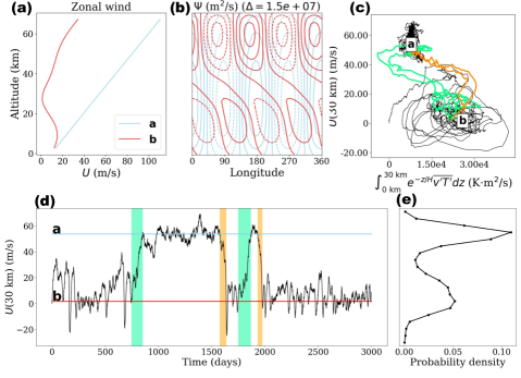
Figure 1: Illustration of the two stable states of the Holton-Mass model and transitions between them. (a) Zonal wind profiles of the radiatively maintained strong vortex (the fixed point $\mathbf{a}$, blue) which increases linearly with altitude, and the weak vortex (the fixed point $\mathbf{b}$, red) which dips close to zero in the mid-stratosphere. (b) Streamfunction contours are overlaid for the two equilibria $\mathbf{a}$ and $\mathbf{b}$. (c) Parametric plot of a control simulation in a 2-dimensional state space projection, including two transitions from $A$ to $B$ (orange) and $B$ to $A$ (green). (d) Time series of $U(30$ km) from the same simulation. (e) The steady state density projected onto $U(30\,\mathrm{km})$.

The two equilibria can be interpreted as two different winter climatologies, one with a strong vortex and one with a weak vortex susceptible to vacillation cycles. To explore transitions between these two states, we follow Birner and Williams (2008) and modify the Holton-Mass equations with small additive noise in the $U$ variable to mimic momentum perturbations by smaller scale Rossby waves, gravity waves, and other unresolved sources. The form of noise will be specified in Eq. (7).

While the details of the additive noise are ad hoc, the general approach can be more rigorously justified through the Mori-Zwanzig formalism (Zwanzig, 2001). Because many hidden degrees of freedom are being projected onto the low-dimensional space of the Holton-Mass model, the dynamics on small observable subspaces can be considered stochastic. This is the perspective taken in stochastic parameterization of turbulence and other high-dimensional chaotic systems (Hasselmann, 1976; DelSole and Farrell, 1995; Franzke and Majda, 2006; Majda et al., 2001; Gottwald et al., 2016). In general, unobserved deterministic dynamics can make the system non-Markovian, which technically violates the assumptions of our methodology. However, with sufficient separation of timescales the Markovian assumption is not unreasonable. Furthermore, memory terms can be ameliorated by lifting data back to higher-dimensional state space with time-delay embedding (Berry et al., 2013; Thiede et al., 2019; Lin and Lu, 2021).

We follow Holton and Mass (1976) and discretize the equations using a finite-difference method in $z$, with 27 vertical levels (including boundaries). After constraining the boundaries, there are $d=3\times(27-2)=75$ degrees of freedom in the model. Christiansen (2000) investigated higher resolution and found negligible differences. The full discretized state is represented by a long vector

$$\mathbf{X}(t)=\Big{[} \text{Re}\{\Psi\}(\Delta z,t),\ldots,\text{Re}\{\Psi\}(z_{top}-\Delta z,t),$$

$$\text{Im}\{\Psi\}(\Delta z,t),\ldots,\text{Im}\{\Psi\}(z_{top}-\Delta z,t),$$ (5)

$$U(\Delta z,t),\ldots,U(z_{top}-\Delta z,t)\Big{]}\in\mathbb{R}^{d}=\mathbb{R}^{75}$$

The deterministic system can be written $d\mathbf{X}(t)/dt=\bm{v}(\mathbf{X}(t))$ for a vector field $\bm{v}:\mathbb{R}^{d}\to\mathbb{R}^{d}$ specified by discretizing (2) and (3). Under deterministic dynamics, $\mathbf{X}(t)\to\mathbf{a}$ or $\mathbf{X}(t)\to\mathbf{b}$ as $t\to\infty$ depending on initial conditions. The addition of white noise changes the system into an Itô diffusion

$$d\mathbf{X}(t)=\bm{v}(\mathbf{X}(t))\,dt+\bm{\sigma}(\mathbf{X}(t))\,d\mathbf{W}(t)$$ (6)

where $\bm{\sigma}:\mathbb{R}^{d}\to\mathbb{R}^{d\times m}$ imparts a correlation structure to the vector $\mathbf{W}(t)\in\mathbb{R}^{m}$ of independent standard white noise processes. As discussed above, we design $\bm{\sigma}$ to be a low-rank, constant matrix that adds spatially smooth stirring to only the zonal wind $U$ (not the streamfunction $\Psi$) and which respects boundary conditions at the bottom and top of the stratosphere. Its structure is defined by the following Euler-Maruyama scheme: in a timesetep $\delta t=0.005$ days, after a deterministic forward Euler step we add the stochastic perturbation to zonal wind on large vertical scales

$$\delta U(z)=\sigma_{U}\sum_{k=0}^{m}\eta_{k}\sin\bigg{[}\bigg{(}k+\frac{1}{2}\bigg{)}\pi\frac{z}{z_{top}}\bigg{]}\sqrt{\delta t}$$ (7)

where $\eta_{k}\ (k=0,1,2)$ are independent unit normal samples, $m=2$, and $\sigma_{U}$ is a scalar that sets the magnitudes of entries in $\bm{\sigma}$. In terms of physical units,

$$\sigma_{U}^{2}=\frac{\mathbb{E}[(\delta U)^{2}]}{\delta t}\approx(1\,\text{m/s})^{2}/\text{day}$$ (8)

$\sigma_{U}$ has units of $(L/T)/T^{1/2}$, where the square-root of time comes from the quadratic variation of the Wiener process. It is best interpreted in terms of the daily root-mean-square velocity perturbation of $1.0$ m/s. We have experimented with this value, and found that reducing the noise level below $0.8$ dramatically reduces the frequency of transitions, while increasing it past $1.5$ washes out metastability. We keep $\sigma_{U}$ constant going forward as a favorable numerical regime to demonstrate our approach, while acknowledging that the specifics of stochastic parameterization are important in general to obtain accurate forecasts. The resulting matrix $\bm{\sigma}$ is $75\times 3$, with nonzero entries only in the last 25 rows as forcing only applies to $U(z)$.

A long simulation of the model reveals metastability, with the system tending to remain close to one fixed point for a long time before switching quickly to the other, as shown by the time series of $U(30\,\text{km})$ in panel (d) of Fig. 1. Panel (e) shows a projection of the steady state distribution, also known as the equilibrium/invariant distribution, of $U$ as a function of $z$. We call this density $\pi(\mathbf{x})$, which is a function over the full $d$-dimensional state space. We focus on the zonal wind $U$ at 30 km following Christiansen (2000), because this is where its strength is minimized in the weak vortex. While the two regimes are clearly associated with the two fixed points, they are better characterized by extended regions of state space with strong and weak vortices. We thus define the two metastable subsets of $\mathbb{R}^{d}$

$$A =\{\mathbf{X}:U(\mathbf{X})(30\,\mathrm{km})\geq U(\mathbf{a})(30\,\mathrm{km})=53.8\,\text{m/s}\},$$

$$B =\{\mathbf{X}:U(\mathbf{X})(30\,\mathrm{km})\leq U(\mathbf{b})(30\,\mathrm{km})=1.75\,\mathrm{m/s}\}.$$

This straightforward definition roughly follows the convention of Charlton and Polvani (2007), which defines an SSW as a reversal of zonal winds at 10 hPa. We use 30 km for consistency with Christiansen (2000); this is technically higher than 10 hPa because $z=0$ in the Holton-Mass model represents the tropopause. Our method is equally applicable to any definition, and the results are not qualitatively dependent on this choice. Incidentally, the analysis tools we present may be helpful in distinguishing predictability properties between different definitions. In fact, we will show that the height neighborhood of 20 km is actually more salient for predicting the event than wind at the 30-km level, even when the event is defined by wind at 30 km! This emerges from statistical analysis alone, and gives us confidence that essential SSW properties are stable with respect to reasonable changes in definition.

The orange highlights in Fig. 1 (d) begin when the system exits the $A$ region bound for $B$, and end when the system enters $B$. The green highlights start when the system leaves $B$ bound for $A$, and end when $A$ is reached. Note that $A\to B$ transitions, SSWs, are much shorter in duration than $B\to A$ transitions. Fig. 1 (c) shows the same paths, but viewed parametrically in a two-dimensional state space consisting of integrated heat flux or IHF $\int_{0\ \mathrm{km}}^{30\,\mathrm{km}}e^{-z/H}\overline{v^{\prime}T^{\prime}}\,dz$, and zonal wind $U$(30 km). IHF is an informative number because it captures both magnitude and phase information of the streamfunction in the Holton-Mass model:

$$\mathrm{IHF}=\int_{0\ \mathrm{km}}^{30\ \mathrm{km}}e^{-z/H}\overline{v^{\prime}T^{\prime}}\,dz\propto\int_{0\ \mathrm{km}}^{30\ \mathrm{km}}|\Psi|^{2}\frac{\partial{\varphi}}{\partial{z}}\,dz$$ (9)

where $\varphi$ is the phase of $\Psi$. The $A\to B$ and $B\to A$ transitions are again highlighted in orange and green respectively, showing geometrical differences between the two directions. We will refer to the $A\to B$ transition as an SSW event, even though it is more accurately a transition between climatologies according to the Holton-Mass interpretation. The $B\to A$ transition is a vortex restoration event. Our focus in this paper is on predicting these transition events (mainly the $A\to B$ direction) and monitoring their progress in a principled way. In the next section we explain the formalism for doing so.

3 Forecast functions: the committor and lead time statistics

3.1 Defining risk and lead time

We will introduce the quantities of interest by way of example. First, suppose the stratosphere is observed in an initial state $\mathbf{X}(0)=\mathbf{x}$ that is neither in $A$ nor $B$, so $U(\mathbf{b})(30\,\mathrm{km})<U(\mathbf{x})(30\,\mathrm{km})<U(\mathbf{a})(30\,\mathrm{km})$ and the vortex is somewhat weakened, but not completely broken down. We call this intermediate zone $D=(A\cup B)^{\textrm{c}}$ (the complement of the two metastable sets). Because $A$ and $B$ are attractive, the system will soon find its way to one or the other at the first-exit time from $D$, denoted

$$\tau_{D^{\textrm{c}}}=\min\{t\geq 0:\mathbf{X}(t)\in D^{\textrm{c}}\}$$ (10)

Here, $D^{\textrm{c}}$ emphasizes that the process has left $D$, i.e., gone to $A$ or $B$. The first-exit location $\mathbf{X}(\tau_{D^{\textrm{c}}})$ is itself a random variable which importantly determines how the system exits $D$: either $\mathbf{X}(\tau_{D^{\textrm{c}}})\in A$, meaning the vortex restores to radiative equilibrium, or $\mathbf{X}(\tau_{D^{\textrm{c}}})\in B$, meaning the vortex breaks down into vacillation cycles. A fundamental goal of forecasting is to determine the probabilities of these two events, which naturally leads to the definition of the (forward) committor function

$$q^{+}(\mathbf{x}) =\begin{cases}\mathbb{P}_{\mathbf{x}}\{\mathbf{X}(\tau_{D^{\textrm{c}}})\in B\}&\mathbf{x}\in D=(A\cup B)^{\textrm{c}}\\ 0&\mathbf{x}\in A\\ 1&\mathbf{x}\in B\end{cases}$$ (11)

where the subscript $\mathbf{x}$ indicates that the probability is conditional on a fixed initial condition $\mathbf{X}(0)=\mathbf{x}$, i.e., $\mathbb{P}_{\mathbf{x}}\{\cdot\}=\mathbb{P}\{\cdot|\mathbf{X}(0)=\mathbf{x}\}$. The superscript “+” distinguishes the forward committor from the backward committor, an analogous quantity for the time-reversed process which we do not use in this paper. Throughout, we will use capital $\mathbf{X}(t)$ to denote a stochastic process, and lower-case $\mathbf{x}$ to represent a specific point in state space, typically an initial condition, i.e., $\mathbf{X}(0)=\mathbf{x}$. Both are $d=75$-dimensional vectors.

The committor is the probability that the system will be in state $B$ (the disturbed state) next rather than $A$ (the strong vortex state). Hence $q^{+}(\mathbf{x})=0$ if you start in $A$, and is 1 if you are already in $B$. In between (i.e., when $\mathbf{x}\in D$), $q^{+}(\mathbf{x})$ tells you the probability that you will first go to $B$ rather than to $A$. That is, $q^{+}(\mathbf{x})$ tells you the probability that an SSW will happen.

Another important forecasting quantity is the lead time to the event of interest. While the forward committor reveals the probability of experiencing vortex breakdown before returning to a strong vortex, it does not say how long either event will take. Furthermore, even if the vortex is restored first, how long will it be until the next SSW does occur? The time until the next SSW event is denoted $\tau_{B}$, again a random variable, whose distribution depends on the initial condition $\mathbf{x}$. We call $\mathbb{E}_{\mathbf{x}}[\tau_{B}]$ the mean first passage time (MFPT) to $B$. Conversely, we may ask how long a vortex disturbance will persist before normal conditions return; the answer (on average) is $\mathbb{E}_{\mathbf{x}}[\tau_{A}]$, the mean first passage time to $A$. These same quantities have been calculated previously in other simplified models, e.g. Birner and Williams (2008) and Esler and Mester (2019).

$\mathbb{E}_{\mathbf{x}}[\tau_{B}]$ has an obvious shortcoming: it is an average over all paths starting from $\mathbf{x}$, including those which go straight into $B$ (i.e., an orange trajectory in Fig. 1c,d) and the rest which return to $A$ i.e., a green trajectory) and linger there, potentially for a very long time, before eventually re-crossing back into $B$. It is more relevant for near-term forecasting to condition $\tau_{B}$ on the event that an SSW is coming before the strong vortex returns. For this purpose, we introduce the conditional mean first passage time, or lead time, to $B$:

$$\eta^{+}(\mathbf{x}):=\mathbb{E}_{\mathbf{x}}[\tau_{B}|\tau_{B}<\tau_{A}]$$ (12)

which quantifies the suddenness of SSW.

All of these quantities can, in principle, be estimated by direct numerical simulation (DNS). For example, suppose we observe an initial condition $\mathbf{X}(0)=\mathbf{x}$ in an operational forecasting setting, and wish to estimate the probability and lead time for the event of next hitting $B$. We would initialize an ensemble $\{\mathbf{X}_{n}(0)=\mathbf{x},n=1,\ldots,N\}$ and evolve each member forward in time until it hits $A$ or $B$ at the random time $\tau_{n}$. In an explicitly stochastic model, random forcing would drive each member to a different fate, while in a deterministic model their initial conditions would be perturbed slightly. To estimate the committor to $B$, we could calculate the fraction of members that hit $B$ first. Averaging the arrival times ($\tau_{n}$), over only those members gives an estimate of the lead time to $B$. For a single initial condition $\mathbf{x}$ reasonably close to $B$, DNS may be the most economical. But how do we systematically compute $q^{+}(\mathbf{x})$ over all of state space (here 75 variables, but potentially billions of variables in a GCM or other state-of-the-art forecast system)?

For this more ambitious goal, DNS is prohibitively expensive. By definition, transitions between $A$ and $B$ are infrequent. Therefore, if starting from $\mathbf{x}$ far from $B$, a huge number of sampled trajectories ($N$) will be required to observe even a small number ending in $B$, and they may take a long time to get there. If instead we could precompute these functions offline over all of state space, the online forecasting problem would reduce to “reading off” the committor and lead time with every new observation. Achieving this goal is the key point of our paper, and we achieve this using the dynamical Galerkin approximation, or DGA, recipe described by Thiede et al. (2019).

A brute force way to estimate these functions is to integrate the model for a long time until it reaches statistical steady state, meaning it has explored its attractor thoroughly according to the steady state distribution. After long enough, it will have wandered close to every point $\mathbf{x}$ sufficiently often to estimate $q^{+}(\mathbf{x})$ and $\eta^{+}$ robustly as in DNS. We have performed such a “control simulation” of $5\times 10^{5}$ days for validation purposes, but our main contribution in this paper is to compute the forecast functions using only short trajectories with DGA, allowing for massive parallelization. However, we will defer the methodological details to Section 5, and first justify the effort with some results. We visualize the committor and lead time computed from short trajectories and elaborate on their interpretation, utility, and relationship to ensemble forecasting methods.

3.2 Steady state distribution

Before visualizing the committor and lead time, it will be helpful to have a precise notion of the steady state distribution, denoted $\pi(\mathbf{x})$, a probability density that describes the long-term behavior of a stochastic process $\mathbf{X}(t)$. Assuming the system is ergodic, averages over time are equivalent to averages over state space with respect to $\pi$. That is, for any well-behaved function $g:\mathbb{R}^{d}\to\mathbb{R}$,

$$\langle g\rangle_{\pi}:=\lim_{T\to\infty}\frac{1}{T}\int_{0}^{T}g(\mathbf{X}(t))\,dt=\int_{\mathbb{R}^{d}}g(\mathbf{x})\pi(\mathbf{x})\,d\mathbf{x}$$ (13)

For example, if $g(\mathbf{x})=\mathbbm{1}_{S}(\mathbf{x})$ (an indicator function, which is 1 for $\mathbf{x}\in S\subset\mathbb{R}^{d}$ and 0 for $\mathbf{x}\notin S$), Eq. (13) says that the fraction of time spent in $S$ can be found by integrating the density over $S$. The density peaks in Fig. 1(d) indicates clearly that the neighborhoods of $\mathbf{a}$ and $\mathbf{b}$ are two such regions with especially large probability under $\pi$. Note that both sides of (13) are independent of the initial condition, which is forgotten eventually. Short-term forecasts are by definition out-of-equilibrium processes, depending critically on initial conditions; however, $\pi(\mathbf{x})$ is important to us here as a “default” distribution for missing information. If the initial condition is only partially observed, e.g. in only one coordinate, we have no information about the other $d-1$ dimensions, and in many cases the most principled tactic is to assume those other dimensions are distributed according to $\pi$, conditional on the observation.

3.3 Visualizing committor and lead times

The forecasts $q^{+}(\mathbf{x})$ and $\eta^{+}(\mathbf{x})$ are functions of a high-dimensional space $\mathbb{R}^{d}$. However, these degrees of freedom may not all be “observable” in a practical sense, given the sparsity and resolution limits of weather sensors, and visualizing them requires projecting onto reduced-coordinate spaces of dimension 1 or 2. We call these “collective variables” (CVs) following chemistry literature (e.g., Noé and Clementi, 2017), and denote them as vector-valued functions from the full state space to a reduced space, $\bm{\theta}:\mathbb{R}^{d}\to\mathbb{R}^{k}$, where $k=1$ or $2$. For instance, Fig. 1 (c) plots trajectories in the CV space consisting of integrated heat flux and zonal wind at 30 km: $\bm{\theta}(\mathbf{x})=\Big{(}\int_{0\ \mathrm{km}}^{30\,\mathrm{km}}e^{-z/H}\overline{v^{\prime}T^{\prime}}\,dz,U(30\,\mathrm{km})\Big{)}$. The first component is a nonlinear function involving products of $\text{Re}\{\Psi\}$ and $\text{Im}\{\Psi\}$, while the second component is a linear function involving only $U$ at a certain altitude. For visualization in general, we have to approximate a function $F:\mathbb{R}^{d}\to\mathbb{R}$, such as the committor or lead time, as a function of reduced coordinates. That is, we wish to find $f:\mathbb{R}^{k}\to\mathbb{R}$ such that $F(\mathbf{x})\approx f(\bm{\theta}(\mathbf{x}))$. Given a fixed CV space $\bm{\theta}$, an “optimal” $f$ is chosen by minimizing some function-space metric between $f\circ\bm{\theta}$ and $F$.

A natural choice is the mean-squared error weighted by the steady state distribution $\pi$, so the projection problem is to minimize over functions $f:\mathbb{R}^{k}\to\mathbb{R}$ the penalty

$$S[f;\bm{\theta}]: =\lVert f\circ\bm{\theta}-F\rVert_{L^{2}(\pi)}^{2}$$

$$=\int_{\mathbb{R}^{d}}\Big{[}f(\bm{\theta}(\mathbf{x}))-F(\mathbf{x})\Big{]}^{2}\pi(\mathbf{x})\,d\mathbf{x}.$$ (14)

The optimal $f$ for this purpose is the conditional expectation

$$f(\mathbf{y}) =\mathbb{E}_{\mathbf{X}\sim\pi}[F(\mathbf{X})|\bm{\theta}(\mathbf{X})=\mathbf{y}]$$

$$=\lim_{|d\mathbf{y}|\to 0}\frac{\int f(\mathbf{x})\mathbbm{1}_{d\mathbf{y}}(\bm{\theta}(\mathbf{x}))\pi(\mathbf{x})\,d\mathbf{x}}{\int\mathbbm{1}_{d\mathbf{y}}(\bm{\theta}(\mathbf{x}))\pi(\mathbf{x})\,d\mathbf{x}}$$ (15)

where $d\mathbf{y}$ is a small neighborhood about $\mathbf{y}$ in CV space $R^{k}$. The subscript $\mathbf{X}\sim\pi$ means that the expectation is with respect to a random variable $\mathbf{X}$ distributed according to $\pi(\mathbf{x})$, i.e., at steady state. Fig. 2 uses this formula to display one-dimensional projections of the committor (first row) and lead time (second row), as well as the one-standard deviation envelope incurred by projecting out the other 74 degrees of freedoom. This “projection error” is defined as the square root of the conditional variance

$$V_{F}(\mathbf{y})=\mathbb{E}_{\mathbf{X}\sim\pi}\Big{[}\Big{(}F(\mathbf{X})-f(\mathbf{y})\Big{)}^{2}\Big{|}\bm{\theta}(\mathbf{X})=\mathbf{y}\Big{]}.$$ (16)

Each quantity is projected onto two different one-dimensional CVs: $U(30\ \mathrm{km})$ (first column) and IHF (second column). In panel (a), for example, we see the committor is a decreasing function of $U$: the weaker the wind, the more likely a vortex breakdown. Moreover, the curve provides a conversion factor between risk (as measured by probability) and a physical variable, zonal wind. An observation of $U(30\ \mathrm{km})=38$ m/s implies a 50% chance of vortex breakdown. The variation in slope also tells us that a wind reduction from 40 m/s to 30 m/s represents a far greater increase in risk than a reduction from 30 m/s to 20 m/s. Meanwhile, panel (b) shows the committor to be an increasing function of IHF, since SSW is associated with large wave amplitude and phase lag. However, IHF seems inferior to zonal wind as a committor proxy, as a small change in IHF from $\sim 15000$ to $\sim 20000$ K$\cdot$m²/s corresponds to a sharp increase in committor from nearly zero to nearly one. In other words, knowing only IHF doesn’t provide much useful information about the threat of SSW until it is already virtually certain. The dotted envelope is also wider in panel (b) than (a), indicating that projecting the committor onto IHF removes more information than projecting onto $U$. While the underlying noise makes it impossible to divine the outcome with certainty from any observation, the projection error clearly privileges some observables over others for their predictive power.

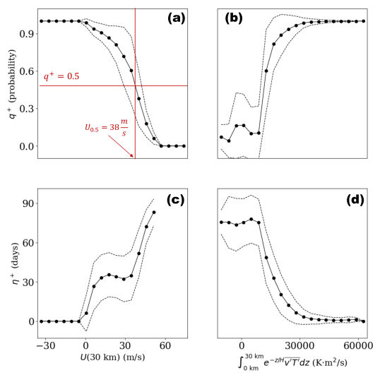
Figure 2: One-dimensional projections of the forward committor (first row) and lead time to $B$ (second row). These functions depend on all $d=75$ degrees of freedom in the model, but we have averaged across $d-1=74$ dimensions to visualize them as rough functions of two single degrees of freedom: $U(30$ km) (first column) and integrated heat flux up to 30 km, IHF (second column). Panel (a) additionally marks the $q^{+}=\frac{1}{2}$ threshold and the corresponding value of zonal wind.

In panels (c) and (d), the lead time is seen to have the opposite overall trend as the committor: the weaker the wind, or the greater the heat flux, the closer you are on average to a vortex breakdown. $\eta^{+}(\mathbf{x})$ is not defined when wind is strongest, as $\mathbf{x}\in A$ and so $q^{+}(\mathbf{x})=0$. However, an interesting exception to the trend occurs in the range $10\ \mathrm{m/s}\leq U\leq 40\ \mathrm{m/s}$: the expected lead time stays constant or slightly decreases as zonal wind increases, and the projection error remains large. This means that while the probability of vortex breakdown increases rapidly from 50% to 90%, the time until vortex breakdown remains highly uncertain. To resolve this seeming paradox, we will have to visualize the joint variation of $q^{+}$ and $\eta^{+}$.

It is of course better to consider multiple observables at once. Fig. 3 shows the information gained beyond observing $U(30\ \mathrm{km})$ by incorporating IHF as a second observable. In the top row we project $\pi$, $q^{+}$, and $\eta^{+}$ onto the two-dimensional subspace, revealing structure hidden from view in the one-dimensional projections. Panel (a) is a 2-dimensional extension of Fig. 1(d), with density peaks visible in the neighborhoods of $\mathbf{a}$ and $\mathbf{b}$. The white space surrounding the gray represents physically insignificant regions of state space that was not sampled by the long simulation. The same convention holds for the following two-dimensional figures. The committor is displayed in panel (b) over the same space. It changes from blue at the top (an SSW is unlikely) to red at the bottom (an SSW is likely), bearing out the negative association between $U$ and $q^{+}$. However, there are non-negligible horizontal gradients that show that IHF plays a role, too. Likewise, the lead time in panel (c) decreases from $\sim 90$ days near $\mathbf{a}$ to 0 days near $\mathbf{b}$, when the transition is complete. Here, IHF appears even more critically important for forecasting how the event plays out, as gradients in $\eta^{+}$ are often completely horizontal.

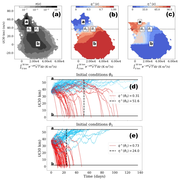
Figure 3: The density, committor, and lead time as functions of zonal wind and integrated heat flux. Panel (a) projects the steady state distribution $\pi(\mathbf{x})$ onto the two-dimensional subspace ($U$,IHF) at 30 km. The white regions surrounding the gray are unphysical states with negligible probability. Panels (b) and (c) display the committor and lead time in the same space. A horizontal transect marks the level $U$(30 km) = 38.5 m/s, where $q^{+}$ according to $U$ only is 0.5. Panels (d) and (e) show ensembles initialized from two points $\bm{\theta}_{0}$ and $\bm{\theta}_{1}$ along the transect, verifying that their committor and lead time values differ from their values according to $U$, in a way that is predictable due to considering IHF in addition to $U$.

A horizontal dotted line in Fig. 3(a-c) marks the 50% risk level $U(30\ \mathrm{km})=38$ m/s, but the committor varies along it from low risk at the left to high risk at the right: we show this concretely by selecting two points $\bm{\theta}_{0}$ and $\bm{\theta}_{1}$ along the line. According to $U$ alone, i.e., the curve in Fig. 2(a), both would have the same committor of 0.5. According to both $U$ and IHF together, i.e., the two-dimensional heat map in Fig. 3(b), they have very different probabilities of $q^{+}(\bm{\theta}_{0})=0.31$ and $q^{+}(\bm{\theta}_{1})=0.73$: an SSW is more than twice as likely to occur from starting point $\bm{\theta}_{1}$ as $\bm{\theta}_{0}$.

While those committor values come from the DGA method to be described in Section 5, we confirm them empirically by plotting an ensemble of 100 trajectories originating from each of the two initial conditions in panels (d) and (e) below, coloring $A$-bound trajectories blue and $B$-bound trajectories red. Only 28% of the sampled trajectories through $\bm{\theta}_{0}$ exhibit an SSW, next going to state $B$, while 68% of the integrations from $\bm{\theta}_{1}$ end at $B$. In both cases, the heatmaps and ensemble sample means roughly match. The small differences between the projected committor and the empirical “success” rate of trajectories arises both from errors in the DGA calculation (which we analyze in section 5) and the finite size of the ensemble.

The lead time prediction is improved similarly by incorporating the second observable. According to $U$ alone, Fig. 2 predicts a lead time of $40$ days for both $\bm{\theta}_{0}$ and $\bm{\theta}_{1}$. Considering IHF additionally, the two-dimensional heat map in Fig. 3 predicts a lead time of 52 days and 24 days for $\bm{\theta}_{0}$ and $\bm{\theta}_{1}$, respectively. Referring to the ensemble from $\bm{\theta}_{1}$ in panels (d) and (e), the arrival times of red trajectories to $B$ provide a discrete sampling of the lead time distributions of $\tau_{B}|\tau_{B}<\tau_{A}$. The sample means are 50 and 32 days respectively from $\bm{\theta}_{0}$ and $\bm{\theta}_{1}$, again roughly matching with our predictions.

These two-dimensional projections still leave out 73 remaining dimensions, which we could incorporate to make the forecasts even better. After accounting for all 75 dimensions, we would obtain the full committor function $q^{+}:\mathbb{R}^{d}\to\mathbb{R}$. This is still a probability, i.e., an expectation over the unresolved turbulent processes and uncertain initial condition. Low-dimensional committor projections simply treat the projected-out dimensions as random variables sampled according to $\pi$. Whether projected to a space of 1 or 75 dimensions, the committor is the function of that space that is closest, in the mean-square sense, to the binary indicator $\mathbbm{1}_{B}(\mathbf{X}(\tau))$; this is the defining characteristic of conditional expectation (Durrett, 2013). In the case that the system does hit $B$ next, the lead time is closest in the mean-square sense to $\tau_{B}$.

While high-dimensional systems offer many coordinates to choose from, we argue that the committor and lead time are the most important nonlinear coordinates to monitor for forecasting purposes. We will explore their relationship in the next subsection. Although both encode some version of proximity to SSW, they are independent variables which deserve separate consideration.

3.4 Relationship between risk and lead time

A forecast is most useful if it comes sufficiently early (to leave some buffer time before impact) and is sufficiently precise to time your response. For example, in June we can say with certainty it will snow next winter in Minnesota. To be useful, we want to know the date of the first snow as early as possible. By relating levels of risk (quantified by $q^{+}$) and lead time (quantified by $\eta^{+}$), we can now assess the limits of early prediction. Such a relationship would answer two questions: for an SSW transition, (1) how far in advance will we be aware of it with some prescribed confidence, say 80%? (2) given some prescribed lead time, say 42 days, how aware or ignorant could we be of it?

The committor and lead time have an overall negative relationship, but they do not completely determine each other, as the contours in Fig. 3(a,b) do not perfectly line up. We treat them as independent variables in Fig. 4, which maps zonal wind and IHF as functions of the coordinates $q^{+}$ and $\eta^{+}$ in an inversion of Fig. 3. The density $\pi(\mathbf{x})$ projected on this space in 4(a) shows again a bimodal structure around $\mathbf{a}$ and $\mathbf{b}$, which occupy opposite corners of this space by construction. Meanwhile, zonal wind and IHF are indicated by the shading in panels (b) and (c). The bridge between $\mathbf{a}$ and $\mathbf{b}$ is not a narrow band, but rather includes a curious high-committor, high-lead time branch which seems paradoxical: points at $q^{+}=0.9$ have a greater spread in $\eta^{+}$ than points at $q^{+}=0.5$, contrary to the intuition that closeness to $B$ in probability means closeness in time. The color shading shows that $q^{+}$ is strongly associated with $U$(30 km), while $\eta^{+}$ is more strongly associated with IHF(30 km). In particular the horizontal contours in panel (c) show that the large spread in lead time near $B$ is due almost completely to variation in IHF. In other words, the system can be highly committed to $B$ with a low zonal wind, but if IHF is low, it may take a long time to get there. We can also see this from the lower-left region of Fig. 3(a) and (b), where committor is high and lead time is high.

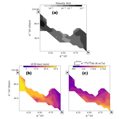
Figure 4: Committor and lead time as independent coordinates. This figure inverts the functions in Fig. 3, considering the zonal wind and integrated heat flux as functions of committor and lead time. The two-dimensional space they span is the essential goal of forecasting. Panel (a) shows the steady state distribution on this subspace, which is peaked near $\mathbf{a}$ and $\mathbf{b}$ (darker shading), weaker in the ”bridge” region between them, and completely negligible the white regions unexplored by data. Panels (b) and (c) display zonal wind and heat flux in color as functions of the committor and lead time.

There are two complementary explanations for this phenomenon. First, the low-$U$, low-IHF region of state space corresponds to a temporary restoration phase in a vacillation cycle, which delays the inevitable collapse of zonal wind below the threshold defining $B$. In fact, the ensemble of pathways starting from $\bm{\theta}_{0}$ in Fig. 3(c) has several members whose zonal wind either stagnates at medium strength, or dips low and partially restores before finally plunging all the way down. The second explanation is that many of these partial restoration events are not part of an $A\to B$ transition, but rather a $B\to B$ transition. In a highly irreversible system such as the Holton-Mass model, these two situations are quite dynamically distinct. To distinguish them using DGA, we would have to account for the past as well as the future, calculating backward-in-time forecasts such as the backward committor $q^{-}(\mathbf{x})=\mathbb{P}_{\mathbf{x}}\{\mathbf{X}(\tau^{-})\in A\}$, where $\tau^{-}<0$ is the most-recent hitting time. Backward forecasts will be analyzed thoroughly in a forthcoming paper, but they are beyond the scope of the present one.

In summary, $q^{+}$ and $\eta^{+}$ are principled metrics to inform preparation for extreme weather. For example, a threatened community might decide in advance to start taking action when an event is very likely, $q^{+}\geq 0.8$, and somewhat imminent, $\eta^{+}\leq 10$ days, or rather, when an event is somewhat likely, $q^{+}\geq 0.5$, and very imminent, $\eta^{+}\leq 3$ days. Because of partial restoration events, the committor does not determine the lead time or vice versa, and so a good real-time disaster response strategy should take both of them into account, defining an “alarm threshold” that is not a single number, but some function of both the committor and lead time. This idea is similar in spirit to that of the Torino scale, which assigns a single risk metric to an asteroid or comet impacts based on both probability and severity (Binzel, 2000). Of course, after many near-SSW events, a lot of material damage may have already occurred, which may be a reason to define a higher threshold for the definition of $B$, or even a continuum for different severity levels of SSW. We emphasize that the choice of $A$, $B$ and alarm thresholds are more of a community and policy decision than a scientific one. The strength of our approach is that it provides a flexible numerical framework to quantify and optimize the consequences of those decisions.

4 Sparse representation of the committor

The committor projections showed give only an impression of its high-dimensional structure. While Eq. (15) says how to optimally represent the committor over a given CV subspace, optimizing $S[f;\bm{\theta}]$ over $f$, it does not say which subspace $\bm{\theta}$ is optimal. If the committor does admit a sparse representation, we could specifically target observations on these high-impact signals. In this section we address this much harder problem of optimizing $S[f;\bm{\theta}]$ over subspaces $\bm{\theta}$.

The set of CV spaces is infinite, as observables $\bm{\theta}$ can be arbitrarily complex nonlinear functions of the basic state variables $\mathbf{x}$. Machine learning algorithms such as artificial neural networks are designed exactly for that purpose: to represent functions nonparametrically from observed input-output pairs. However, to keep the representation interpretable, we will restrict ourselves to physics-informed input features based on the Eliassen-Palm (EP) relation, which relates wave activity, PV fluxes and gradients, and heating source terms in a conservation equation. From Yoden (1987b), the EP relation for the Holton-Mass model takes the form

$$\partial_{t}\bigg{(}\frac{q^{\prime 2}}{2}\bigg{)} +(\partial_{y}\overline{q})\rho_{s}^{-1}\nabla\cdot\bm{F}$$

$$=-\frac{f_{0}^{2}}{N^{2}}\rho_{s}^{-1}\overline{q^{\prime}\partial_{z}(\alpha\rho_{s}\partial_{z}\psi^{\prime})}$$ (17)

$$\text{ where }\bm{F}=(-\rho_{s}\overline{u^{\prime}v^{\prime}}) \mathbf{j}+(\rho_{s}\overline{v^{\prime}\partial_{z}\psi^{\prime}})\mathbf{k}$$

The EP flux divergence has two alternative expressions: $\rho_{s}^{-1}\nabla\cdot\bm{F}=\overline{v^{\prime}q^{\prime}}=\rho_{s}^{-1}\frac{R}{Hf_{0}}\partial_{z}\big{[}\rho_{s}\overline{v^{\prime}T^{\prime}}\big{]}$. If there were no dissipation $(\alpha=0)$ and the background zonal state were time-independent ($\partial_{t}\overline{q}=0$), dividing both sides by $\partial_{y}\overline{q}$ would express local conservation of wave activity $\mathcal{A}=\rho_{s}\overline{q^{\prime 2}}/(2\partial_{y}\overline{q})$. Neither of these is exact in the stochastic Holton-Mass model, so we use the quantities in Eq. (17) as diagnostics: enstrophy $\overline{q^{\prime 2}}$, PV gradient $\partial_{y}\overline{q}$, PV flux $\overline{v^{\prime}q^{\prime}}$, and heat flux $\overline{v^{\prime}T^{\prime}}$. Each field is a function of $(y,z)$ and takes on very different profiles for the states $\mathbf{a}$ and $\mathbf{b}$, as found by Yoden (1987b). A transition from $A$ to $B$, where the vortex weakens dramatically, must entail a reduction in $\partial_{y}\overline{q}$ and a burst in positive $\overline{v^{\prime}T^{\prime}}$ (negative $\overline{v^{\prime}q^{\prime}}$) as a Rossby wave propagates from the tropopause vertically up through the stratosphere and breaks. This is the general physical narrative of a sudden warming event, and these same fields might be expected to be useful observables to track for qualitative understanding and prediction. For visualization, we have found $U(30\,km)$ and IHF(30 km) $=\int_{0\,\mathrm{km}}^{30\,\mathrm{km}}e^{-z/H}\overline{v^{\prime}T^{\prime}}\,dz$ to be particularly helpful. However, this doesn’t necessarily imply they are optimal predictors of $q^{+}$, and regression is a more principled way to find them.

We start by projecting the committor onto each observable at each altitude separately, in hopes of finding particularly salient altitude levels that clarify the role of vertical interactions. The first five rows of Fig. 5 display, for five fields ($U$, $|\Psi|$, $\overline{q^{\prime 2}}$, $\partial_{y}\overline{q}$, and $\overline{v^{\prime}q^{\prime}}$) and for a range of altitude levels, the mean and standard deviation of the committor projected onto that field at that altitude. Each altitude has a different range of the CV; for example, because $U$ has a Dirichlet condition at the bottom and a Neumann condition at the top, the lower levels have a much smaller range of variability than the high levels. We also plot the integrated variance, or $L^{2}$ projection error, at each level in the right-hand column. A low projected committor variance over $U$ at altitude $z_{0}$ means that the committor is mostly determined by the single observable $U(z_{0})$, while a high projected variance indicates significant dependence of $q^{+}$ on variables other than $U(z_{0})$. In order to compare different altitudes and fields as directly as possible, the $L^{2}$ projection error at each altitude is an average over discrete bins of the observable.

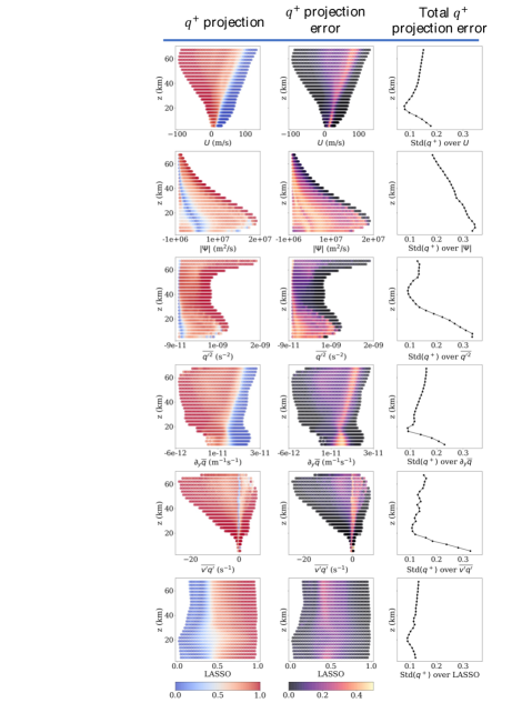
Figure 5: Projection of the forward committor onto a large collection of altitude-dependent physical variables. The top left panel shows heatmaps of $q^{+}$ as a function of $U$ and $z$; white regions denote where $U(z)$ is negligibly observed. The top middle panel shows the standard deviation in $q^{+}$ as a function of $U$ and $z$; this uncertainty stems from the remaining 74 model dimensions. The right-hand panel displays the total mean-squared error due to the projection for each altitude, i.e., $\sqrt{S[f;\bm{\theta}]}$ from Eq. (14). A low value indicates that this level is ideal for prediction. The following rows show the same quantities for other physical variables: streamfunction magnitude, eddy enstrophy, background PV gradient, eddy PV flux, and LASSO.

In selecting good CV’s, we generally look for a simple, hopefully monotonic, and sensitive relationship with the committor. Of all the candidate fields, $U$ and $\partial_{y}\overline{q}$ stand out the most in this respect, being clearly negatively correlated with the forward committor at all altitudes. The associated projection error tends to be greatest in the region $q^{+}\approx 0.5$, as observed before, but interestingly there is a small altitude band around $15-25$ km where its magnitude is minimized. This suggests an optimal altitude for monitoring the committor through zonal wind, giving the most reliable estimate possible for a single state variable. In contrast, the projection of $q^{+}$ onto $|\Psi|$, displays a large variance across all altitudes. The eddy enstrophy and potential vorticity flux are also rather unhelpful as early warning signs, despite their central role in SSW evolution. For example, the large, positive spikes in heat flux across all altitudes generally occur after the committor $\approx 0.5$ threshold has already been crossed. Furthermore, the relationship of $\overline{v^{\prime}q^{\prime}}$ with the committor is not smooth. The $q^{+}<0.5$ region at each altitude is a thin band near zero.

The exhaustive CV search in Fig. 5 is visually compelling in favor of some fields and some altitudes over others, but it is not satisfactory as a rigorous comparison. Differences between units and ranges make it difficult to objectively compare the $L^{2}$ projection error. Furthermore, restricting to one variable at a time is limiting. Accordingly, we also perform a more automated approach to identify salient variables in the form of a generalized linear model for the forward committor, using sparsity-promoting LASSO regression (“Least Absolute Shrinkage and Selection Operator”) due to Tibshirani (1996), as implemented in the scikit-learn Python package (Pedregosa et al., 2011). As input features, we use all state variables $\text{Re}\{\Psi\},\text{Im}\{\Psi\},U$, the integrated heat flux $\int_{0}^{z}e^{-z/H}\overline{v^{\prime}T^{\prime}}\,dz$, the eddy PV flux $\overline{v^{\prime}q^{\prime}}$, and the background PV gradient $\partial_{y}\overline{q}$, at all altitudes $z$ simultaneously. The advantage of a sparsity-promoting regression is that it isolates a small number of observables that can accurately approximate the committor in linear combination. Considering that regions close to $A$ and $B$ have low committor uncertainty, we regress only on data points with $q^{+}\in(0.2,0.8)$, and of those only a subset weighted by $\pi(\mathbf{x})q^{+}(\mathbf{x})(1-q^{+}(\mathbf{x}))$ to further emphasize the transition region $q^{+}\approx 0.5$. To constrain committor predictions to the range $(0,1)$, we regress on the committor after an inverse-sigmoid transformation, $\ln(q^{+}/(1-q^{+}))$. First we do this at each altitude separately, and in Fig. 6 (a) we plot the coefficients of each component as a function of altitude. The bottom row of Fig. 5 also displays the committor projected on the height-dependent LASSO predictor.

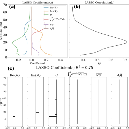
Figure 6: Results of LASSO regression of the forward committor with linear and nonlinear input features. Panel (a) shows the coefficients when $q^{+}$ is regressed as a function of only the variables at a given altitude, and panel (b) shows the corresponding correlation score. 21.5 km seems the most predictive (where $z\equiv 0$ at the tropopause, not the surface). Panel (c) shows the coefficient structure when all altitudes are considered simultaneously. Most of the nonzero coefficients appear between 15-22 km, distinguishing that range as highly relevant for prediction.

The height-dependent regression in 6(a) shows each component is salient for some altitude range. In general, $U$ and $\text{Im}\{\Psi\}$ dominate as causal variables at low altitudes, while $\text{Re}\{\Psi\}$ dominates at high altitudes. The overall prediction quality, as measured by $R^{2}$ and plotted in Fig. 6 (b), is greatest around 21.5 km, consistent with our qualitative observations of Fig. 5. Note that not all single-altitude slices are sufficient for approximating the committor, even with LASSO regression; in the altitude band $50-60$ km, the LASSO predictor is not monotonic and has a large projected variance, as seen in the bottom row of Fig. 5. The specific altitude can matter a great deal. But by using all altitudes at once, the committor approximation may be improved further. We thus repeat the LASSO with all altitudes simultaneously and find the sparse coefficient structure shown in 6 (c), with a few variables contributing the most, namely the state variables $\Psi$ and $U$ in the altitude range 15-22 km. The nonlinear CVs failed to make any nonzero contribution to LASSO, and this remained stubbornly true for other nonlinear combinations not shown, such as $\overline{v^{\prime}T^{\prime}}$. With multiple lines of evidence indicating 21.5 km as an altitude with high predictive value for the forward committor, we can make a strong recommendation for targeting observations here. This conclusion applies only to the Holton-Mass model under these parameters, but the methodology explained above can be applied similarly to models of arbitrary complexity.

We have presented the committor and lead time as “ideal” forecasts, especially the committor, which we have devoted considerable effort to approximating in this section. We want to emphasize that $q^{+}$ and $\eta^{+}$ are not competitors to ensemble forecasting; rather, they are two of its most important end results. So far, we have simply advocated including $q^{+}$ and $\eta^{+}$ as quantities of interest. Going forward, however, we do propose an alternative to ensemble forecasting aimed specifically at the committor, lead time, and a wider class of forecasting functions, as they are important enough in their own right to warrant dedicated computation methods. Our approach uses only short simulations, making it highly parallelizable, and shifts the numerical burden from online to offline. Figs. 2-6 were all generated using the short-simulation algorithm. While the method is not yet optimized and in some cases not competitive with ensemble forecasting, we anticipate such methods will be increasingly favorable with modern trends in computing.

5 The computational method

In this section we describe the methodology, which involves some technical results from stochastic processes and measure theory. After describing the theoretical motivation and the numerical pipeline in turn, we demonstrate the method’s accuracy and discuss its efficiency compared to straightforward ensemble forecasting.

5.1 Feynman-Kac formulae

The forecast functions described above—committors and passage times—can all be derived from general conditional expectations of the form

$$F(\mathbf{x};\lambda) =\mathbb{E}_{\mathbf{x}}\bigg{[}G(\mathbf{X}(\tau))\exp\bigg{(}\lambda\int_{0}^{\tau}\Gamma(\mathbf{X}(s))\,ds\bigg{)}\bigg{]}$$ (18)

where again the subscript $\mathbf{x}$ denotes conditioning on $\mathbf{X}(0)=\mathbf{x}$; $G,\Gamma$ are arbitrary known functions over $\mathbb{R}^{d}$; and $\tau$ is a stopping time, specifically a first-exit time like Eq. (10) but possibly with $D$ replaced by another set. $\lambda$ is a variable parameter that turns $F$ into a moment-generating function. To see that the forward committor takes on this form, set $G(\mathbf{x})=\mathbbm{1}_{B}(\mathbf{x})$, $\lambda=0$ ($\Gamma$ can be anything), and $\tau=\tau_{A\cup B}$. Then $F(\mathbf{x})=\mathbb{E}_{\mathbf{x}}\big{[}\mathbbm{1}_{B}(\mathbf{X}(\tau))\big{]}=\mathbb{P}_{\mathbf{x}}\{\mathbf{X}(\tau_{D^{c}})\in B\}=q^{+}(\mathbf{x})$. For the $\eta^{+}$, set $\tau=\tau_{B}$, $G=\mathbbm{1}_{B}$, and $\Gamma=1$. Then

$$F(\mathbf{x};\lambda) =\mathbb{E}_{\mathbf{x}}\big{[}\mathbbm{1}_{B}(\mathbf{X}(\tau))\exp(\lambda\tau)\big{]}$$ (19)

$$\frac{1}{q^{+}(\mathbf{x})}\frac{\partial{}}{\partial{\lambda}}F(\mathbf{x};0) =\frac{\mathbb{E}_{\mathbf{x}}[\tau\mathbbm{1}_{B}(\mathbf{X}(\tau))]}{\mathbb{E}_{\mathbf{x}}[\mathbbm{1}_{B}(\mathbf{X}(\tau))]}$$ (20)

$$=\eta^{+}(\mathbf{x}).$$ (21)

So we must also be able to differentiate $F$ with respect to $\lambda$.

More generally, the function $G$ is chosen by the user to quantify risk at the terminal time $\tau$; in the case of the forward committor, that risk is binary, with an SSW representing a positive risk and a radiative vortex no risk at all. The function $\Gamma$ is chosen to quantify the risk accumulated up until time $\tau$, which might be simply an event’s duration, but other integrated risks may be of more interest for the application. For example, one could express the total poleward heat flux by setting $\Gamma=\overline{v^{\prime}T^{\prime}}$, or the momentum lost by the vortex by setting $\Gamma(\mathbf{x})=U(\mathbf{a})-U(\mathbf{x})$. Extending (20), one can compute not only means but higher moments of such integrals by expressing the risk with $\Gamma$. Repeated differentiation of $F(\mathbf{x};\lambda)$ gives

$$\partial_{\lambda}^{k}F(\mathbf{x};0) =\mathbb{E}_{\mathbf{x}}\bigg{[}G(\mathbf{X}(\tau))\bigg{(}\int_{0}^{\tau}\Gamma(\mathbf{X}(s))\,ds\bigg{)}^{k}\bigg{]}$$ (22)

We choose to focus on expectations of the form (18) in order to take advantage of the Feynman-Kac formula, which represents $F(\mathbf{x};\lambda)$ as the solution to a PDE boundary value problem over state space. As PDEs involve local operators, this form is more amenable to solution with short trajectories which don’t stray far from their source. The boundary value problem associated with (18) is

$$\begin{cases}(\mathcal{L}+\lambda\Gamma)F(\mathbf{x};\lambda)=0&\mathbf{x}\in D\\ F(\mathbf{x};\lambda)=G(\mathbf{x})&\mathbf{x}\in D^{\textrm{c}}\end{cases}$$ (23)

The domain $D$ here is some combination of $A^{\textrm{c}}$ and $B^{\textrm{c}}$. The operator $\mathcal{L}$ is known as the infinitesimal generator of the stochastic process, which acts on functions by pushing expectations forward in time along trajectories:

$$\mathcal{L}f(\mathbf{x}):=\lim_{\Delta t\to 0}\frac{\mathbb{E}_{\mathbf{x}}[f(\mathbf{X}(\Delta t))]-f(\mathbf{x})}{\Delta t}$$ (24)

In a diffusion process like the stochastic Holton-Mass model, $\mathcal{L}$ is an advection-diffusion partial differential operator which is analogous to a material derivative in fluid mechanics. The generator encapsulates the properties of the stochastic process. In addition to solving boundary value problems (18), its adjoint $\mathcal{L}^{*}$ provides the Fokker-Planck equation for the stationary density $\pi(\mathbf{x})$:

$$\mathcal{L}^{*}\pi(\mathbf{x})=0$$ (25)

We can also write equations for moments of $F$, as in (22), by differentiating (23) repeatedly and setting $\lambda=0$:

$$\mathcal{L}\big{[}\partial_{\lambda}^{k}F\big{]}(\mathbf{x};0) =-k\Gamma\partial_{\lambda}^{k-1}F$$ (26)

This is an application of the Kac Moment Method (Fitzsimmons and Pitman, 1999). Note that we never actually have to solve (23) with nonzero $\lambda$. Instead we implement the recursion above. Note that the base case, $k=0$, with $G=\mathbbm{1}_{B}$ gives $F^{+}=q^{+}$, no matter what the risk function $\Gamma$. In this paper we compute only up to the first moment, $k=1$. Further background regarding stochastic processes and Feynman-Kac formulae can be found in Karatzas and Shreve (1998); Oksendal (2003); E et al. (2019).

5.2 Dynamical Galerkin Approximation

To solve the boundary value problem (23) with $\lambda=0$, we start by following the standard finite element recipe, converting to a variational form and projecting onto a finite basis. First, we homogenize boundary conditions by writing $F(\mathbf{x})=\hat{F}(\mathbf{x})+f(\mathbf{x})$, where $\hat{F}$ is a guess function that obeys the boundary condition $\hat{F}|_{D^{\textrm{c}}}=G$, and $f|_{D^{\textrm{c}}}=0$. Next, we integrate the equation against any test function $\phi$, weighting the integrand by a density $\mu$ (which is arbitrary for now, but will be specified later):

$$\int_{\mathbb{R}^{d}}\phi(\mathbf{x})\mathcal{L}f(\mathbf{x})\mu(\mathbf{x})\,d\mathbf{x} =\int\phi(\mathbf{x})(G-\mathcal{L}\hat{F})(\mathbf{x})\mu(\mathbf{x})d\mathbf{x}$$

$$\langle\phi,\mathcal{L}f\rangle_{\mu} =\langle\phi,G-\mathcal{L}\hat{F}\rangle_{\mu}$$ (27)

The test function $\phi$ should live in the same space as $f$, i.e., with homogeneous boundary conditions $\phi(\mathbf{x})=0$ for $\mathbf{x}\in A\cup B$. We refer to the inner products in (27) as being “with respect to” the measure (with density) $\mu$. We approximate $f$ by expanding in a finite basis $f(\mathbf{x})=\sum_{j=1}^{M}\xi_{j}\phi_{j}(\mathbf{x})$ with unknown coefficients $\xi_{j}$, and enforce that (27) hold for each $\phi_{i}$. This reduces the problem to a system of linear equations,

$$\sum_{j=1}^{M}\langle\phi_{i},\mathcal{L}\phi_{j}\rangle_{\mu}\xi_{j} =\langle\phi_{i},G-\mathcal{L}\hat{F}\rangle_{\mu} i=1,\ldots,M$$ (28)

which can be solved with standard numerical linear algebra packages.

This procedure consists of three crucial subroutines. First, we must construct a set of basis functions $\phi_{j}$. Second, we have to evaluate the generator’s action on them, $\mathcal{L}\phi_{j}$. Third, we have to compute inner products. With standard PDE methods, the basis size would grow exponentially with dimension, quickly rendering the first and third steps intractable. Successful approaches will involve a representation of the solution, $F$, suitable for the high dimensional setting, i.e. representations of the type commonly employed for machine learning tasks. DGA is one such method, whose special twist is to construct a “data-informed” basis of reasonable size, evaluate the generator by implementing Eq. (24) with the same data set, and finally evaluate the inner products (27) with a Monte Carlo integral. The data consist of short trajectories launched from all over state space, which the system of linear equations stitches together into a global function estimate. We sketch the procedure here, but for the implementation details we refer to the appendix and to Thiede et al. (2019) and Strahan et al. (2021), where DGA has already been developed for molecular dynamics.

Step 1: Generate the data, in the format of $N$ initial conditions $\{\mathbf{X}_{n}:1\leq n\leq N\}$. Evolve each initial condition forward for a “lag time” $\Delta t$ to obtain a set of short trajectories $\{\mathbf{X}_{n}(t):0\leq t\leq{\Delta t},n=1,\ldots,N\}\subset\mathbb{R}^{d}$. (Lag time is an algorithmic parameter for DGA. It is not to be confused with the forecast time horizon between the prediction and the event of interest in meteorology.) Here and going forward, $\mathbf{X}_{n}$ will mean $\mathbf{X}_{n}(0)$. The choice of starting points is flexible, but crucial for the efficiency and accuracy of DGA. Because our goal here is to demonstrate interpretable results, we prioritize simplicity and accuracy over efficiency, and defer optimization to later work. We simply draw initial conditions at random from the long control simulation of $5\times 10^{5}$ days, and then generate new short trajectories from those points. We do not sample the points with equal probability, but instead re-weight to get a uniform distribution over the space $(U(30\,\mathrm{km}),|\Psi|(30\,\mathrm{km}))$, within the bounds realized by the control simulation, which are approximately $-30\,\mathrm{m/s}\leq U(30\,\mathrm{km})\leq 70$ m/s and $0\,\text{m}^{2}/\text{s}\leq|\Psi|(30\,\text{km})\leq 2\times 10^{7}\,\text{m}^{2}/\text{s}$. This sampling procedure, and any other version, implicitly defines a sampling measure $\mu$ on state space, where $\mu(\mathbf{x})\,d\mathbf{x}$ is the expected fraction of starting points in the neighborhood $d\mathbf{x}$ about $\mathbf{x}$. Sampling points with equal weight from the control run would induce $\mu=\pi$, a very inefficient choice because probability concentrates around the metastable states $\mathbf{a}$ and $\mathbf{b}$. The re-weighting procedure ensures data coverage of intermediate-wind regions between $A$ and $B$, as well as the large bursts of wave amplitude that characterize the transition pathways. Our main results use $N=5\times 10^{5}$ short trajectories with a lag time of $\Delta t=20$ days, sampled at a frequency of twice per day. This data set is more than needed to get a reasonable committor estimate, but we have sampled generously in order to visualize the functions in high detail. The final section will show the method is robust, capable of reasonably approximating the committor even with an order-of-magnitude reduction in data.

Step 2: Define the basis. The Galerkin method works for any class of basis functions that becomes increasingly expressive as the library grows and becomes capable of estimating any function of interest. However, with a finite truncation, choosing basis functions is a crucial ingredient of DGA, greatly impacting the efficiency and accuracy of the results. In our current study, we restrict to the simplest kind of basis, which consists of indicator functions $\phi_{i}(x)=\mathbbm{1}_{S_{i}}(x)$, where $\{S_{1},\ldots,S_{M}\}$ is a disjoint partition of state space. In practice we will construct these sets by clustering the initial data points as described in more detail in Appendix A. This is a common practice in the computational statistical mechanics community for building a Markov State Model (MSM) (Chodera et al., 2006; Frank and Fischer, 2008; Pande et al., 2010; Bowman et al., 2013; Chodera and Noé, 2014). MSMs are a dimensionality reduction technique that has also been used in conjuction with analysis of metastable transitions, primarily in protein folding dynamics (Jayachandran et al., 2006; Noé et al., 2009). MSMs have also been used recently to study garbage patch dynamics in the ocean (Miron et al., 2021) as well as complex social dynamics (Helfmann et al., 2021). In Maiocchi et al. (2020), the authors take an interesting approach to MSMs by clustering points based on proximity to unstable periodic orbits, a potentially useful paradigm for general chaotic weather phenomena (Lucarini and Gritsun, 2020). DGA can be viewed as an extension of MSMs, though, rather than producing any reduced complexity model, the explicit goal in DGA is estimating specific functions as in Eq. (18).

Step 3: Apply the generator. The forward difference formula

$$\widehat{\mathcal{L}\phi}(\mathbf{X}_{n})=\frac{\phi(\mathbf{X}_{n}(\Delta t))-\phi(\mathbf{X}_{n})}{\Delta t}$$ (29)

suggested by the definition of the generator (24), results in a systematic bias when $\Delta t$ is finite. On the other hand, small values of $\Delta t$ lead to large variances in our Monte Carlo estimates of the inner products in (28). To resolve these issues we use an integrated form of the Feynman–Kac equations that involves stopping trajectories when they enter $A$ or $B$. Details are provided in Appendix A.

Step 4: Compute the inner products. The inner products in Eq. (28) are integrals over high-dimensional state space that are intractable with standard quadrature, but can be approximated using Monte Carlo integration. If $\mathbf{X}$ is an $\mathbb{R}^{d}$-valued random variable distributed according to $\mu$, and we have access to random samples $\{\mathbf{X}_{1},\ldots,\mathbf{X}_{N}\}$ (which we do), the law of large numbers gives, for any function $g$ with finite expectation,

$$\lim_{N\to\infty}\frac{1}{N}\sum_{n=1}^{N}g(\mathbf{X}_{n})=\int_{\mathbb{R}^{d}}g(\mathbf{x})\mu(\mathbf{x})d\mathbf{x}$$ (30)

Setting $g(\mathbf{x})=\phi_{i}(\mathbf{x})\mathcal{L}\phi_{j}(\mathbf{x})$, the sample average on the left-hand side of (30) therefore provides an estimator of $\langle\phi_{i},\mathcal{L}\phi_{j}\rangle_{\mu}$. Of course, our approximation uses finite $N$ and nonzero $\Delta t$. A similar sample average approximation can be used to estimate the inner product on the right-hand side of (28).

These same steps apply to both $q^{+}$ and $\mathbb{E}[\tau_{B}]$, as well as the recursion in (26) for $\eta^{+}$. For the Fokker-Planck equation (25), one extra step is needed to convert an equation with $\mathcal{L}^{*}$ into an equation with $\mathcal{L}$. Our procedure for estimating $\pi$ is described in Appendix A.

Step 5: Solve the equation (28). With a reasonable basis size $M\lesssim 1000$, an $LU$ solver such as in LAPACK via Numpy can handle Eq. (28). In the case of the homogeneous system for $w(\mathbf{x})$, a $QR$ decomposition can identify the null vector.

5.3 DGA fidelity and sensitivity analysis

To illustrate the effect of parameter choices on performance, we present here a simple sensitivity analysis. Fig. 7 verifies the numerical accuracy and convergence of DGA by plotting the committor as a function of $U$(30 km), estimated both with DNS and DGA, for various DGA parameters. The red curves $q^{+}_{\text{DGA}}(U(30\,\text{km}))$ are calculated by projecting the committor as in Fig. 2(a), while the black curve $q^{+}_{\text{DNS}}(U(30\,\mathrm{km}))$ is an empirical committor estimate equal to the fraction of control simulation points seen at a particular value of $U(30\,\mathrm{km})$ that next hit $B$.

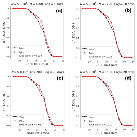
Figure 7: Fidelity of DGA. For several DGA parameter values of $N$ (the number of data points), $M$ (the number of basis functions) and lag time, we plot the committor calculated from DGA and DNS (from the long control simulation), both as a function of $U$(30 km). The mean-square difference $\varepsilon$ in the legend is used as a global error estimate for DGA.

In panels (a), (b), and (d), the lag time $\Delta t$ increases from 5 to 10 to 20 days while the number of short trajectories stays fixed at $N=5\times 10^{5}$. Panel (c) has a long lag of 20 days, but a small data set of $N=5\times 10^{4}$, allowing us to see the tradeoff between $N$ and $\Delta t$. The basis size $M$ is chosen heuristically as large as possible within reason for the clustering algorithm (see Appendix A). While DGA tends to systematically overestimate $q^{+}$ relative to $q^{+}_{\text{DNS}}$ in the mid-range of $U$, it seems to approach the empirical estimate as the data size and lag time increase. Each plot also displays the root-mean-square deviation between the two estimators over this subspace, $\varepsilon=\sqrt{\big{\langle}(q^{+}_{\text{DGA}}-q^{+}_{\text{DNS}})^{2}\big{\rangle}_{\pi}}$. Within this regime, it seems that increasing the lag time has a greater impact on the deviation than increasing the number of data points. Panels (b) and (c) have approximately the same deviation $\varepsilon$, but (c) uses only one fifth the data, measured by total simulation time. On the other hand, more short trajectories can be parallelized more readily than fewer long trajectories, and the optimal choice will depend on computing resources.

It is natural to ask whether our short trajectory based approach is more efficient than DNS in which many independent “long” trajectories are launched from a single initial condition $\mathbf{x}$ and the committor probability $q^{+}(\mathbf{x})$ (or another forecast) is estimated directly. For a single value of $\mathbf{x}$ for which $q^{+}(\mathbf{x})$ is not very small (so that a non-negligible fraction of trajectories reach $B$ before $A$) and for which the lead time $\eta^{+}(\mathbf{x})$ is not too large (so that trajectories reaching $B$ do so without requiring long integration times), DNS will undoubtedly be more efficient. This is often the situation in real-time weather forecasting. However, a key feature of our approach is that it simultaneously estimates forecasts at all values of $\mathbf{x}$, allowing the subsequent analysis of those functions that has been the focus of much of this article. Global knowledge of the committor and lead time is more pertinent for oft-repeated forecasts, for long-term risk assessment of extreme event climatology, and for targeting observations optimally. Building accurate estimators in all of state space by DNS would be extremely costly even for the reduced complexity model studied here.

6 Conclusion

Forecasting rare events is, by the very nature of rare events, an extremely difficult computational task, and one of science’s most pressing challenges. We have described a computational framework, a dynamical Galerkin approximation to the Feynman-Kac equations, that combines the minimalistic philosophy of dimensionality reduction with the fidelity of high-resolution models. We identify a set of reduced coordinates, the committor probability and expected lead time, that provide the essential information that large ensemble forecasts hope to compute. DGA uses relatively short simulations of the full model to estimate these quantities of interest, allowing for prediction on much longer timescales than that of the simulation. In its focus on directly estimating statistics of interest, DGA differs from previous reduced-order modeling methods that attempt to capture general qualities of the system, including both physics-based models (Lorenz, 1963; Charney and DeVore, 1979; Legras and Ghil, 1985; Crommelin, 2003; Timmermann et al., 2003; Ruzmaikin et al., 2003) and more recent data-driven models making use of machine learning (Giannakis and Majda, 2012; Giannakis et al., 2018; Berry et al., 2015; Sabeerali et al., 2017; Majda and Qi, 2018; Wan et al., 2018; Bolton and Zanna, 2019; Chattopadhyay et al., 2020; Chen and Majda, 2020; Kashinath et al., 2021; Chattopadhyay et al., 2021).

We have shown numerical results in the context of a stochastically forced Holton-Mass model with 75 degrees of freedom, which points to the method’s promise for forecasting. By systematically evaluating many model variables for their utility in predicting the fate of the vortex, we have identified some salient physical descriptions of early warning signs. We have furthermore examined the relationship between probability and lead time for a given rare event, a powerful pairing for assessing predictability and preparing for extreme weather. Our results suggest that the slow evolution of vortex preconditioning is an important source of predictability. In particular, the zonal wind and streamfunction in the range of 10-20 km above the tropopause seems to be optimal among a large class of dynamically motivated observables.

Beyond the problem of real-time weather forecasting, it is also important to assess the climatology, i.e., long-term frequency, intensity, and other characteristics of rare events. For this goal as well, our methodology offers advantages over large ensemble simulations, which are currently the most detailed source of data (e.g., Schaller et al., 2018). The committor and lead time are ingredients in a larger framework called Transition Path Theory (TPT) for describing rare transition events at steady state, meaning average properties over long timescales. TPT describes not only the future evolution from an initial condition ($\mathbf{x}\to B$), but the ensemble of full vortex breakdown events ($A\to B$), and how they differ from restoration events ($B\to A$). In principle, interrogating the ensemble of transition paths requires direct simulation of the system long enough to observe many transition events. However, using TPT, quantities computable by our framework can be combined to yield key statistics describing the ensemble of transition paths (Metzner et al., 2006, 2009; Vanden-Eijnden and E, 2010; E. and Vanden-Eijnden, 2006; Finkel et al., 2020). In a following paper we will apply the same short-trajectory forecasting approach together with TPT to compute transition path statistics such as return times and extract insight about physical mechanisms of the transition process.

Scaling our approach up to state-of-the-art weather and climate models will require significant further development. In particular, a completely new procedure for generating trajectory initial conditions will need to be introduced. Generation of a trajectory long enough to thoroughly sample transitions will not be practical for more complicated models. One promising alternative is launching many trajectories in parallel and selectively replicating those that explore new regions of state space, especially transition regions. Such an approach could build on exciting progress over the last decade in targeted rare event simulation schemes (Hoffman et al., 2006; Weare, 2009; Bouchet et al., 2011, 2014; Vanden-Eijnden and Weare, 2013; Chen et al., 2014; Yasuda et al., 2017; Farazmand and Sapsis, 2017; Dematteis et al., 2018; Mohamad and Sapsis, 2018; Dematteis et al., 2019; Webber et al., 2019; Bouchet et al., 2019a, b; Plotkin et al., 2019; Simonnet et al., 2020; Ragone and Bouchet, 2020; Sapsis, 2021). A potential challenge here is that GCMs may not be set up for short simulations that start and stop frequently. For this reason, it may be sensible to use longer lag times and a sliding window to define short trajectories. Furthermore, the communication overhead required for adaptive sampling with GCMs would impose additional costs. We have deferred the sampling problem to future work, acknowledging that this step is crucial to make DGA competitive. The utility of committor and lead time, however, is independent of the method for computing them.

Defining the source of stochasticity is also an important step that varies between models. Explicitly stochastic parameterization (e.g., Berner et al., 2009; Porta Mana and Zanna, 2014) will automatically lead to a spread in the short-trajectory ensemble, but in deterministic models, uncertainty will arise from perturbing the initial conditions. This may require special care depending on the model.

Another area of algorithmic improvement is selecting a basis expansion of the forecast functions. In upcoming work we will explore more flexible representations using kernel methods and neural networks. The solution of high-dimensional PDEs is an active research area that is making innovative use of machine learning, particularly in the fields of computational chemistry, quantum mechanics, and fluid dynamics (e.g., Carleo and Troyer, 2017; Han et al., 2018; Khoo et al., 2018; Li et al., 2020; Mardt et al., 2018; Li et al., 2019; Raissi et al., 2019; Lorpaiboon et al., 2020; Rotskoff and Vanden-Eijnden, 2020). Similar approaches may hold great potential for understanding predictability in atmospheric science.

$$\mathcal{L}f(\mathbf{x}) =\lim_{\Delta t\to 0}\frac{\mathbb{E}_{\mathbf{x}}[f(\mathbf{X}(\Delta t))]-f(\mathbf{x})}{\Delta t}$$ (31)

where $\mathbb{E}_{\mathbf{x}}[\cdot]:=\mathbb{E}[\cdot|\mathbf{X}(0)=\mathbf{x}]$. It can be shown that under the above assumptions on $\mathbf{X}$, the Itô chain rule gives

$$df(\mathbf{X}(t)) =\mathcal{L}f(\mathbf{X}(t))\,dt+d\mathbf{M}(t)$$ (32)

where $\mathbf{M}(t)$ is a martingale. More concretely, in this paper, $\mathbf{X}(t)$ is an Itô diffusion obeying the stochastic differential equation

$$\mathbf{X}(t)=\mathbf{X}(0) +\int_{0}^{t}b(\mathbf{X}(s))\,ds$$ (33)

$$+\int_{0}^{t}\bm{\sigma}(\mathbf{X}(s))\,d\mathbf{W}(s)$$

with infinitesimal generator and martingale terms

$$\mathcal{L}f(\mathbf{x}) =\sum_{i=1}^{d}b_{i}(\mathbf{x})\frac{\partial{f(\mathbf{x})}}{\partial{\mathbf{x}_{i}}}$$ (34)

$$\hskip 5.69046pt+\sum_{i=1}^{d}\sum_{j=1}^{d}\frac{1}{2}\big{[}\sigma(\mathbf{x})\sigma(\mathbf{x})^{\top}\big{]}_{ij}\frac{\partial^{2}f(\mathbf{x})}{\partial\mathbf{x}_{i}\partial\mathbf{x}_{j}}$$

$$d\mathbf{M}(t) =\sum_{i=1}^{d}\frac{\partial{f(\mathbf{x})}}{\partial{\mathbf{x}_{i}}}\sigma_{ij}(\mathbf{x})d\mathbf{W}_{j}(t)$$ (35)

The key forecasting quantities in this paper are of the form  (18) and can be solved with  (23), a linear equation involving the generator. We now lay out a brief derivation of the Feynman-Kac formula and our numerical discretization, roughly following E et al. (2019).

.1 Feynman-Kac formula

Let $D$ be a domain in $\mathbb{R}^{d}$ (for example, $(A\cup B)^{c}$) and $\tau_{D^{\textrm{c}}}=\min\{t\geq 0:\mathbf{X}(t)\notin D\}$ be the first exit time from this domain starting at time zero. This is a random variable which depends on the starting condition $\mathbf{x}\in D$. Let $G:\partial D\to\mathbb{R}$ be a boundary condition, $\Gamma:D\to\mathbb{R}$ a source term, and $\Gamma:D\to\mathbb{R}$ a term to represent accumulated risk. We seek a PDE for the conditional expectation from  (18):

$$F(\mathbf{x})=\mathbb{E}_{\mathbf{x}}\bigg{[} G(\mathbf{X}(\tau))\exp\bigg{(}\lambda\int_{0}^{\tau}\Gamma(\mathbf{X}(s))\,ds\bigg{)}\bigg{]}$$ (36)

where $\mathbb{E}_{\mathbf{x}}[\cdot]=\mathbb{E}[\cdot|\mathbf{X}(0)=\mathbf{x}]$. To derive the PDE  (23), consider the following stochastic process:

$$Z(t) =F(\mathbf{X}(t))Y(t)$$ (37)

where $Y(t):=\exp\big{(}\lambda\int_{0}^{t}\Gamma(\mathbf{X}(s))\,ds\big{)}$. Itô’s lemma gives us that $dY(t)=\lambda\Gamma(\mathbf{X}(t))Y(t)\,dt$. Hence, applying the product rule to $Z(t)$,

$$dZ(t) =dF(\mathbf{X}(t))Y(t)+F(\mathbf{X}(t))\,dY(t)$$ (38)

$$=\mathcal{L}F(\mathbf{X}(t))Y(t)\,dt+d\mathbf{M}(t)Y(t)$$ (39)

$$\hskip 5.69046pt+\lambda F(\mathbf{X}(t))\Gamma(\mathbf{X}(t))Y(t)\,dt$$

$$=\big{[}\mathcal{L}F+\lambda\Gamma F\big{]}(\mathbf{X}(t))Y(t)\,dt+Y(t)d\mathbf{M}(t)$$ (40)

where in (38) we have left out the quadratic cross-variation of $F(\mathbf{X}(t))$ and $Y(t)$ because $Y$ has finite variation. If the bracketed term $(\mathcal{L}+\lambda\Gamma(\mathbf{x}))F(\mathbf{x})=0$ for all $\mathbf{x}$, then $Z(t)$ is a martingale and it follows that

$$Z(0) =\mathbb{E}_{\mathbf{x}}[Z(t)]$$ (41)

$$F(\mathbf{x}) =\mathbb{E}_{\mathbf{x}}\bigg{[}F(\mathbf{X}(t))\exp\bigg{(}\lambda\int_{0}^{t}\Gamma(\mathbf{X}(s))\,ds\bigg{)}\bigg{]}$$ (42)

Finally, the formula still holds if we substitute a stopping time for $t$. By choosing $\tau$, the first exit time from $D$, the $F(\mathbf{X}(t))$ inside the brackets becomes its boundary value $G(\mathbf{X}(\tau))$. Thus $F(\mathbf{x})$ as defined in  (36) also solves the PDE boundary value problem (23):

$$\begin{cases}(\mathcal{L}+\lambda\Gamma(\mathbf{x}))F(\mathbf{x};\lambda)=0&\mathbf{x}\in D\\ F(\mathbf{x};\lambda)=G(\mathbf{x})&\mathbf{x}\in D^{\textrm{c}}\end{cases}$$ (43)

where we have inserted the additional dependence of $F$ on $\lambda$ in order to lead directly to the recursive formulas (20) and (26).

.2 Dynkin’s formula and finite lag time

We have presented  (29) as a mathematically concise approximation to the generator. In practice, we achieve better numerical stability integrating the generator (31) to a finite lag time $\Delta t$, following Strahan et al. (2021). The theorem that allows this is called Dynkin’s formula (e.g., Oksendal, 2003), which states that for any suitable function $f:\mathbb{R}^{d}\to\mathbb{R}$ and a stopping time $\theta$ (not to be confused with CV coordinates),

$$\mathbb{E}_{\mathbf{x}}[f(\mathbf{X}(\theta))]=f(\mathbf{x})+\mathbb{E}_{\mathbf{x}}\bigg{[}\int_{0}^{\theta}\mathcal{L}f(\mathbf{X}(t))\,dt\bigg{]}.$$ (44)

The left-hand side, $\mathbb{E}_{\mathbf{x}}[f(\mathbf{X}(\theta))]$, is known as the transition operator $\mathcal{T}^{\theta}f(\mathbf{x})$, a finite-time version of the generator. Note that this is a deterministic operator despite $\theta$ being a random variable, because by definition $\mathcal{T}^{\theta}$ only has $\theta$ inside of expectations. We can apply Dynkin’s formula to (43) before numerical approximation, setting $\theta=\min(\Delta t,\tau)$. That is, the short trajectory $\{\mathbf{X}(t):0\leq t\leq\Delta t=20\text{ days}\}$ is stopped early if it exits the domain $D$ before $\Delta t$. Applying Dynkin’s formula to $F(\mathbf{x};\lambda)$, we find

$$\mathbb{E}_{\mathbf{x}}[F(\mathbf{X}(\theta))] =F(\mathbf{x})+\mathbb{E}_{\mathbf{x}}\bigg{[}\int_{0}^{\theta}\mathcal{L}F(\mathbf{X}(t))\,dt\bigg{]}$$

$$=F(\mathbf{x})-\lambda\mathbb{E}_{\mathbf{x}}\bigg{[}\int_{0}^{\theta}\Gamma(\mathbf{X}(t))F(\mathbf{X}(t))\,dt\bigg{]}$$

$$\mathcal{T}^{\theta}F(\mathbf{x}) =F(\mathbf{x})-\lambda\mathcal{I}^{\theta}[\Gamma F](\mathbf{x})$$ (45)

where $\mathcal{I}^{\theta}$ is shorthand notation for the integral operator on the right. Eq. (45), along with the boundary conditions $F|_{D^{\textrm{c}}}=G|_{D^{\textrm{c}}}$, gives us a linear equation for $F(\mathbf{x})$ that can be solved by DGA. As outlined in Section 5, we write $F=\hat{F}+f$, where $\hat{F}$ obeys the boundary conditions and $f$ obeys

$$(\mathcal{T}^{\theta}-1)f(\mathbf{x}) +\lambda\mathcal{I}^{\theta}[\Gamma f](\mathbf{x})=$$ (46)

$$-(\mathcal{T}^{\theta}-1)\hat{F}(\mathbf{x})-\lambda\mathcal{I}^{\theta}[\Gamma\hat{F}](\mathbf{x})$$

We then expand $f=\sum_{j=1}^{M}\xi_{j}\phi_{j}(\mathbf{x})$ with basis functions $\{\phi_{j}\}$ that are zero on $D^{\textrm{c}}$, and take $\mu$-weighted inner products with $\phi_{i}$ on both sides to obtain

$$\sum_{j=1}^{M}\xi_{j}\Big{(}\big{\langle} \phi_{i},(\mathcal{T}^{\theta}-1)\phi_{j}\big{\rangle}_{\mu}+\lambda\big{\langle}\phi_{i},\mathcal{I}^{\theta}[\Gamma\phi_{j}]\big{\rangle}_{\mu}\Big{)}=$$

$$-\big{\langle}\phi_{i},(\mathcal{T}^{\theta}-1)\hat{F}\big{\rangle}_{\mu}-\lambda\big{\langle}\phi_{i},\mathcal{I}^{\theta}[\Gamma\hat{F}]\big{\rangle}_{\mu}$$ (47)

Finally, the inner products can be estimated with short trajectories using (30). For two functions $\phi$ and $\psi$, the first left-hand side inner product is approximately

$$\big{\langle}\phi,(\mathcal{T}^{\theta}-1)\psi\big{\rangle}_{\mu} \approx\frac{1}{N}\sum_{n=1}^{N}\phi(\mathbf{X}_{n})\big{[}\psi(\mathbf{X}_{n}(\theta_{n}))-\psi(\mathbf{X}_{n})\big{]}$$ (48)

where $\theta_{n}$ is the sampled first-exit time of the $n$th trajectory, or $\Delta t$ if it never exits. The second left-hand side inner product is approximately

$$\big{\langle}\phi, \mathcal{I}^{\theta}[\Gamma\psi]\big{\rangle}_{\mu}\approx$$

$$\frac{1}{N}\sum_{n=1}^{N}\phi(\mathbf{X}_{n})\int_{0}^{\theta_{n}}\Gamma(\mathbf{X}_{n}(t))\psi(\mathbf{X}_{n}(t))\,dt$$ (49)

where the time integral on the right is computed with the trapezoid rule on the trajectory, which is sampled every $0.5$ days. The error from numerical quadrature is likely small compared to the error from basis set construction, but higher-order integration methods do merit further investigation.

Given a fixed $\Gamma$ and $G$, and with the inner products in hand, we now have (47) as a family of matrix equations with $\lambda$ a continuous parameter:

$$(P+\lambda Q)\bm{\xi}(\lambda)=\mathbf{v}+\lambda\mathbf{r}.$$ (50)

We can then differentiate in $\lambda$ and evaluate at $\lambda=0$ to obtain a ready-to-solve discretization of the recursion (26):

$$P\bm{\xi}(0) =\mathbf{v}$$ (51)

$$P\bm{\xi}^{\prime}(0) =\mathbf{r}-Q\xi(0)$$ (52)

$$P\bm{\xi}^{(k)}(0) =-kQ\bm{\xi}^{(k-1)}(0)\text{ for }k\geq 2$$ (53)

where the $k$’th derivative $\bm{\xi}^{(k)}(0)$ is the coefficient expansion in the basis $\{\phi_{j}\}$ of the $k$’th moment from (22):

$$\partial_{\lambda}^{k}F(\mathbf{x};0) =\mathbb{E}_{\mathbf{x}}\bigg{[}G(\mathbf{X}(\tau))\bigg{(}\lambda\int_{0}^{\tau}\Gamma(\mathbf{X}(s))\,ds\bigg{)}^{k}\bigg{]}$$ (54)

.3 Change of measure

We now specify how to compute the change of measure from $\mu$ (the sampling distribution) to $\pi$ (the steady-state distribution), using an adjoint version of the Feynman-Kac formula. Each of the basis functions $\phi_{i}$ has an expectation at time zero with respect to the steady state distribution: $\mathbb{E}_{\mathbf{X}(0)\sim\pi}[\phi_{i}(\mathbf{X}(0))]=\int\phi_{i}(\mathbf{x})\pi(\mathbf{x})\,d\mathbf{x}$. Evolving the dynamics from $0$ to $\Delta t$ induces another expectation: $\mathbb{E}_{\mathbf{X}(0)\sim\pi}[\phi_{i}(\mathbf{X}(\Delta t))]=\int\mathcal{T}^{\Delta t}\phi_{i}(\mathbf{x})\pi(d\mathbf{x})$. $\pi$ is the invariant distribution, which means that these two integrals are equal:

$$\int(\mathcal{T}^{\Delta t}-1)\phi_{i}(\mathbf{x})\pi(\mathbf{x})d\mathbf{x}=0.$$ (55)

Furthermore, with a change of measure they can be rewritten with respect to the sampling measure $\mu$ instead of $\pi$, so

$$\int(\mathcal{T}^{\Delta t}-1)\phi_{i}(\mathbf{x})\frac{d{\pi}}{d{\mu}}(\mathbf{x})\mu(\mathbf{x})\,d\mathbf{x}=0$$ (56)

The change of measure $\frac{d{\pi}}{d{\mu}}(\mathbf{x})$, which we abbreviate $w(\mathbf{x})$, is yet another unknown function which we expand in the basis as $w(\mathbf{x})=\sum_{j}\xi_{j}\phi_{j}(\mathbf{x})$. Putting this into the integral and using Monte Carlo, we cast the coefficients $\xi_{j}$ as the solution to a null eigenvector problem:

$$0 =\int(\mathcal{T}^{\Delta t}-1)\phi_{i}(\mathbf{x})\sum_{j=1}^{M}\xi_{j}\phi_{j}(\mathbf{x})\mu(d\mathbf{x})$$ (57)

$$\approx\sum_{j=1}^{M}\xi_{j}\sum_{n=1}^{N}\big{[}\phi_{i}(\mathbf{X}_{n}(\Delta t))-\phi_{i}(\mathbf{X}_{n})\big{]}\phi_{j}(\mathbf{X}_{n})$$ (58)

This last equation is simply the Fokker-Planck equation, $\mathcal{L}^{*}\pi=0$, in weak form and integrated in time using Dynkin’s formula. Note that the matrix elements in (58) are the transpose of those in (48).

.4 DGA details

We will provide more details here on our particular construction of basis functions. The partition $\{S_{1},\ldots,S_{M}\}$ to build the basis function library $\phi_{j}(\mathbf{x})=\mathbbm{1}_{S_{j}}(\mathbf{x})$, $n=1,\ldots,N$ should be chosen with a number of considerations in mind. The partition elements should be small enough to accurately represent the functions they are used to approximate, but large enough to contain sufficient data to robustly estimate transition probabilities. We form these sets by a hierarchical modification of $K$-means clustering on the initial points $\{\mathbf{X}_{n}\}_{n=1}^{N}$. $K$-means is a robust method that can incorporate new samples by simply identifying the closest centroid, and is commonly used in molecular dynamics (Pande et al., 2010). However, straightforward application of $K$-means, as implemented in the scikit-learn software (Pedregosa et al., 2011), can produce a very imbalanced cluster size distribution, even with empty clusters. This leads to unwanted singularities in the constructed Markov matrix. To avoid this problem we cluster hierarchically, starting with a coarse clustering of all points and iteratively refining the larger clusters, at every stage enforcing a minimum cluster size of five points, until we have the desired number of clusters ($M$). After clustering on the initial points $\{\mathbf{X}_{n}\}$, the other points $\{\mathbf{X}_{n}(t),0<t\leq\Delta t\}$ are placed into clusters using an address tree produced by the $K$-means cluster hierarchy. For boundary value problems with a domain $D$ and boundary $D^{\textrm{c}}$, we need only cluster points in $D$, since the basis should be homogeneous. The total number of clusters should scale with data set. In our main results with $N=5\times 10^{5}$, we found $M=1500$ to be enough basis functions to resolve some of the finer details in the structure of the forecast functions, but not so many as to require an unmanageably deep address tree, which manifests in dramatic slowdown past a certain threshold. At this point, the cluster number is still a manually tuned hyperparameter.

Because the committor and lead time obey Dirichlet boundary conditions on $A\cup B$, the basis funtions used to construct them should be zero on $A\cup B$, meaning only data points $\mathbf{X}_{n}\notin A\cup B$ should be used to produce the clusters. On the other hand, the steady state distribution has no boundary condition to satisfy, only a global normalization condition. Hence, the basis for the change of measure $w$ must be different from the basis for $q^{+}$ and $\eta^{+}$, with its clusters including all data points in $A\cup B$. Furthermore, the basis must be chosen so that the matrix $\langle(\mathcal{T}^{\Delta t}-1)\phi_{i},\phi_{j}\rangle$ has a nontrivial null space; this is guaranteed by the indicator basis set we use, but can otherwise be guaranteed by including a constant function in the basis.

The use of an indicator basis follows the Markov State Modeling literature (Chodera et al., 2006; Pande et al., 2010, e.g.,), which has the advantage of simplicity and robustness. In particular, the discretization of $\mathcal{T}^{\theta}-1$ is a properly normalized stochastic matrix (with nonnegative entries and rows summing to 1), which guarantees the maximum principle $0\leq q^{+}(\mathbf{x})\leq 1$ and $0\leq w(\mathbf{x})$ for all data points $\mathbf{x}$. However, alternative basis sets have been shown to be promising, perhaps with much less data. Thiede et al. (2019) used diffusion maps, while Strahan et al. (2021) used a PCA-like procedure to construct the basis. More generally, there is no requirement to use a linear Galerkin method to solve the Feynman-Kac formulae. More flexible functional forms may have an important role to play as well. In the low-data regime, some preliminary experiments have suggested that Gaussian process regression (GPR) is a useful way to constrain the committor estimate with a prior, following the framework in Bilionis (2016) to solve PDEs with Gaussian processes. As mentioned in the conclusion, there is rapidly growing interest in the use of artificial neural networks to solve PDEs. As with many novel methods, however, DGA is likely to work best on new applications when its simplest form is applied first. This will be our approach in coming experiments on more complex models.

References

- Berner et al. (2009) Berner, J., G. J. Shutts, M. Leutbecher, and T. N. Palmer, 2009: A spectral stochastic kinetic energy backscatter scheme and its impact on flow-dependent predictability in the ecmwf ensemble prediction system. Journal of the Atmospheric Sciences, 66 (3), 603 – 626, 10.1175/2008JAS2677.1, URL https://journals.ametsoc.org/view/journals/atsc/66/3/2008jas2677.1.xml.
- Berry et al. (2013) Berry, T., J. R. Cressman, Z. Gregurić-Ferenček, and T. Sauer, 2013: Time-scale separation from diffusion-mapped delay coordinates. SIAM Journal on Applied Dynamical Systems, 12 (2), 618–649, 10.1137/12088183X, URL https://doi.org/10.1137/12088183X, https://doi.org/10.1137/12088183X.
- Berry et al. (2015) Berry, T., D. Giannakis, and J. Harlim, 2015: Nonparametric forecasting of low-dimensional dynamical systems. Phys. Rev. E, 91, 032 915, 10.1103/PhysRevE.91.032915.
- Bilionis (2016) Bilionis, I., 2016: Probabilistic solvers for partial differential equations. arXiv: Probability.
- Binzel (2000) Binzel, R. P., 2000: The torino impact hazard scale. Planetary and Space Science, 48 (4), 297–303, https://doi.org/10.1016/S0032-0633(00)00006-4, URL https://www.sciencedirect.com/science/article/pii/S0032063300000064.
- Birner and Williams (2008) Birner, T., and P. D. Williams, 2008: Sudden stratospheric warmings as noise-induced transitions. Journal of the Atmospheric Sciences, 65 (10), 3337–3343, 10.1175/2008JAS2770.1.
- Bolton and Zanna (2019) Bolton, T., and L. Zanna, 2019: Applications of deep learning to ocean data inference and subgrid parameterization. Journal of Advances in Modeling Earth Systems, 11 (1), 376–399, https://doi.org/10.1029/2018MS001472, URL https://agupubs.onlinelibrary.wiley.com/doi/abs/10.1029/2018MS001472, https://agupubs.onlinelibrary.wiley.com/doi/pdf/10.1029/2018MS001472.
- Bouchet et al. (2011) Bouchet, F., J. Laurie, and O. Zaboronski, 2011: Control and instanton trajectories for random transitions in turbulent flows. Journal of Physics: Conference Series, 318 (2), 022 041, 10.1088/1742-6596/318/2/022041, URL https://doi.org/10.1088%2F1742-6596%2F318%2F2%2F022041.
- Bouchet et al. (2014) Bouchet, F., J. Laurie, and O. Zaboronski, 2014: Langevin dynamics, large deviations and instantons for the quasi-geostrophic model and two-dimensional euler equations. Journal of Statistical Physics, 156, 1066–1092, 10.1007/s10955-014-1052-5, URL https://doi.org/10.1007/s10955-014-1052-5.
- Bouchet et al. (2019a) Bouchet, F., J. Rolland, and E. Simonnet, 2019a: Rare event algorithm links transitions in turbulent flows with activated nucleations. Physical Review Letters, 122 (7), 074 502, 10.1103/PhysRevLett.122.074502.
- Bouchet et al. (2019b) Bouchet, F., J. Rolland, and J. Wouters, 2019b: Rare event sampling methods. Chaos: An Interdisciplinary Journal of Nonlinear Science, 29 (8), 080 402, 10.1063/1.5120509.
- Bowman et al. (2013) Bowman, G. R., V. S. Pande, and F. Noé, 2013: An introduction to Markov state models and their application to long timescale molecular simulation, Vol. 797. Springer Science & Business Media.
- Carleo and Troyer (2017) Carleo, G., and M. Troyer, 2017: Solving the quantum many-body problem with artificial neural networks. Science, 355 (6325), 602–606, 10.1126/science.aag2302, URL https://science.sciencemag.org/content/355/6325/602, https://science.sciencemag.org/content/355/6325/602.full.pdf.
- Charlton and Polvani (2007) Charlton, A. J., and L. M. Polvani, 2007: A new look at stratospheric sudden warmings. part i: Climatology and modeling benchmarks. Journal of Climate, 20 (3), 449–469, 10.1175/JCLI3996.1.
- Charney and DeVore (1979) Charney, J. G., and J. G. DeVore, 1979: Multiple Flow Equilibria in the Atmosphere and Blocking. Journal of the Atmospheric Sciences, 36 (7), 1205–1216, 10.1175/1520-0469(1979)036¡1205:MFEITA¿2.0.CO;2, URL https://doi.org/10.1175/1520-0469(1979)036¡1205:MFEITA¿2.0.CO;2, https://journals.ametsoc.org/jas/article-pdf/36/7/1205/3420739/1520-0469(1979)036“˙1205“˙mfeita“˙2“˙0“˙co“˙2.pdf.
- Chattopadhyay et al. (2021) Chattopadhyay, A., M. Mustafa, P. Hassanzadeh, E. Bach, and K. Kashinath, 2021: Towards physically consistent data-driven weather forecasting: Integrating data assimilation with equivariance-preserving spatial transformers in a case study with era5. Geoscientific Model Development Discussions, 2021, 1–23, 10.5194/gmd-2021-71, URL https://gmd.copernicus.org/preprints/gmd-2021-71/.
- Chattopadhyay et al. (2020) Chattopadhyay, A., E. Nabizadeh, and P. Hassanzadeh, 2020: Analog forecasting of extreme-causing weather patterns using deep learning. Journal of Advances in Modeling Earth Systems, 12 (2), e2019MS001 958, https://doi.org/10.1029/2019MS001958, URL https://agupubs.onlinelibrary.wiley.com/doi/abs/10.1029/2019MS001958, e2019MS001958 10.1029/2019MS001958, https://agupubs.onlinelibrary.wiley.com/doi/pdf/10.1029/2019MS001958.
- Chen et al. (2014) Chen, N., D. Giannakis, R. Herbei, and A. J. Majda, 2014: An mcmc algorithm for parameter estimation in signals with hidden intermittent instability. SIAM/ASA Journal on Uncertainty Quantification, 2 (1), 647–669, 10.1137/130944977, URL https://doi.org/10.1137/130944977, https://doi.org/10.1137/130944977.
- Chen and Majda (2020) Chen, N., and A. J. Majda, 2020: Predicting observed and hidden extreme events in complex nonlinear dynamical systems with partial observations and short training time series. Chaos: An Interdisciplinary Journal of Nonlinear Science, 30 (3), 033 101, 10.1063/1.5122199, URL https://doi.org/10.1063/1.5122199, https://doi.org/10.1063/1.5122199.
- Chodera and Noé (2014) Chodera, J. D., and F. Noé, 2014: Markov state models of biomolecular conformational dynamics. Current Opinion in Structural Biology, 25, 135 – 144, https://doi.org/10.1016/j.sbi.2014.04.002, URL http://www.sciencedirect.com/science/article/pii/S0959440X14000426, theory and simulation / Macromolecular machines.
- Chodera et al. (2006) Chodera, J. D., W. C. Swope, J. W. Pitera, and K. A. Dill, 2006: Long‐time protein folding dynamics from short‐time molecular dynamics simulations. Multiscale Modeling & Simulation, 5 (4), 1214–1226, 10.1137/06065146X.
- Christiansen (2000) Christiansen, B., 2000: Chaos, quasiperiodicity, and interannual variability: Studies of a stratospheric vacillation model. Journal of the Atmospheric Sciences, 57 (18), 3161–3173, 10.1175/1520-0469(2000)057¡3161:CQAIVS¿2.0.CO;2.
- Crommelin (2003) Crommelin, D. T., 2003: Regime transitions and heteroclinic connections in a barotropic atmosphere. Journal of the Atmospheric Sciences, 60 (2), 229 – 246, 10.1175/1520-0469(2003)060¡0229:RTAHCI¿2.0.CO;2, URL https://journals.ametsoc.org/view/journals/atsc/60/2/1520-0469˙2003˙060˙0229˙rtahci˙2.0.co˙2.xml.
- DelSole and Farrell (1995) DelSole, T., and B. F. Farrell, 1995: A stochastically excited linear system as a model for quasigeostrophic turbulence: Analytic results for one- and two-layer fluids. Journal of the Atmospheric Sciences, 52 (14), 2531–2547, 10.1175/1520-0469(1995)052¡2531:ASELSA¿2.0.CO;2.
- Dematteis et al. (2019) Dematteis, G., T. Grafke, M. Onorato, and E. Vanden-Eijnden, 2019: Experimental evidence of hydrodynamic instantons: The universal route to rogue waves. Phys. Rev. X, 9, 041 057, 10.1103/PhysRevX.9.041057, URL https://link.aps.org/doi/10.1103/PhysRevX.9.041057.
- Dematteis et al. (2018) Dematteis, G., T. Grafke, and E. Vanden-Eijnden, 2018: Rogue waves and large deviations in deep sea. Proceedings of the National Academy of Sciences, 115 (5), 855–860, 10.1073/pnas.1710670115.
- Durrett (2013) Durrett, R., 2013: Probability: Theory and Examples. Cambridge University Press.
- E et al. (2019) E, W., T. Li, and E. Vanden-Eijnden, 2019: Applied stochastic analysis, Vol. 199. American Mathematical Soc.
- E. and Vanden-Eijnden (2006) E., W., and E. Vanden-Eijnden, 2006: Towards a Theory of Transition Paths. Journal of Statistical Physics, 123 (3), 503, 10.1007/s10955-005-9003-9, URL https://doi.org/10.1007/s10955-005-9003-9.
- Esler and Mester (2019) Esler, J. G., and M. Mester, 2019: Noise-induced vortex-splitting stratospheric sudden warmings. Quarterly Journal of the Royal Meteorological Society, 145 (719), 476–494, https://doi.org/10.1002/qj.3443, URL https://rmets.onlinelibrary.wiley.com/doi/abs/10.1002/qj.3443, https://rmets.onlinelibrary.wiley.com/doi/pdf/10.1002/qj.3443.
- Farazmand and Sapsis (2017) Farazmand, M., and T. P. Sapsis, 2017: A variational approach to probing extreme events in turbulent dynamical systems. Science Advances, 3 (9), 10.1126/sciadv.1701533, URL https://advances.sciencemag.org/content/3/9/e1701533, https://advances.sciencemag.org/content/3/9/e1701533.full.pdf.
- Finkel et al. (2020) Finkel, J., D. S. Abbot, and J. Weare, 2020: Path Properties of Atmospheric Transitions: Illustration with a Low-Order Sudden Stratospheric Warming Model. Journal of the Atmospheric Sciences, 77 (7), 2327–2347, 10.1175/JAS-D-19-0278.1, URL https://doi.org/10.1175/JAS-D-19-0278.1, https://journals.ametsoc.org/jas/article-pdf/77/7/2327/4958190/jasd190278.pdf.
- Fitzsimmons and Pitman (1999) Fitzsimmons, P., and J. Pitman, 1999: Kac’s moment formula and the feynman–kac formula for additive functionals of a markov process. Stochastic Processes and their Applications, 79 (1), 117–134, https://doi.org/10.1016/S0304-4149(98)00081-7, URL https://www.sciencedirect.com/science/article/pii/S0304414998000817.
- Frank and Fischer (2008) Frank, N., and S. Fischer, 2008: Transition networks for modeling the kinetics of conformational change in macromolecules. Current Opininion in Structural Biology, 18, 154–163, 10.1016/j.sbi.2008.01.008.
- Franzke and Majda (2006) Franzke, C., and A. J. Majda, 2006: Low-order stochastic mode reduction for a prototype atmospheric gcm. Journal of the Atmospheric Sciences, 63 (2), 457–479, 10.1175/JAS3633.1.
- Giannakis et al. (2018) Giannakis, D., A. Kolchinskaya, D. Krasnov, and J. Schumacher, 2018: Koopman analysis of the long-term evolution in a turbulent convection cell. Journal of Fluid Mechanics, 847, 735–767, 10.1017/jfm.2018.297.
- Giannakis and Majda (2012) Giannakis, D., and A. J. Majda, 2012: Nonlinear laplacian spectral analysis for time series with intermittency and low-frequency variability. Proceedings of the National Academy of Sciences, 109 (7), 2222–2227, 10.1073/pnas.1118984109, https://www.pnas.org/content/109/7/2222.full.pdf.
- Gottwald et al. (2016) Gottwald, G. A., D. T. Crommelin, and C. L. E. Franzke, 2016: Stochastic climate theory. 1612.07474.
- Han et al. (2018) Han, J., A. Jentzen, and W. E, 2018: Solving high-dimensional partial differential equations using deep learning. Proceedings of the National Academy of Sciences, 115 (34), 8505–8510, 10.1073/pnas.1718942115, URL https://www.pnas.org/content/115/34/8505, https://www.pnas.org/content/115/34/8505.full.pdf.
- Hasselmann (1976) Hasselmann, K., 1976: Stochastic climate models part i. theory. Tellus, 28 (6), 473–485, 10.3402/tellusa.v28i6.11316.
- Helfmann et al. (2021) Helfmann, L., J. Heitzig, P. Koltai, J. Kurths, and C. Schütte, 2021: Statistical analysis of tipping pathways in agent-based models. 2103.02883.
- Hoffman et al. (2006) Hoffman, R. N., J. M. Henderson, S. M. Leidner, C. Grassotti, and T. Nehrkorn, 2006: The response of damaging winds of a simulated tropical cyclone to finite-amplitude perturbations of different variables. Journal of the Atmospheric Sciences, 63 (7), 1924 – 1937, 10.1175/JAS3720.1, URL https://journals.ametsoc.org/view/journals/atsc/63/7/jas3720.1.xml.
- Holton and Mass (1976) Holton, J. R., and C. Mass, 1976: Stratospheric vacillation cycles. Journal of the Atmospheric Sciences, 33 (11), 2218–2225, 10.1175/1520-0469(1976)033¡2218:SVC¿2.0.CO;2.
- Jayachandran et al. (2006) Jayachandran, G., V. Vishal, and V. S. Pande, 2006: Using massively parallel simulation and markovian models to study protein folding: Examining the dynamics of the villin headpiece. The Journal of Chemical Physics, 124 (16), 164 902, 10.1063/1.2186317, URL https://doi.org/10.1063/1.2186317, https://doi.org/10.1063/1.2186317.
- Karatzas and Shreve (1998) Karatzas, I., and S. E. Shreve, 1998: Brownian Motion and Stochastic Calculus. Springer.
- Kashinath et al. (2021) Kashinath, K., and Coauthors, 2021: Physics-informed machine learning: case studies for weather and climate modelling. Philosophical Transactions of the Royal Society A: Mathematical, Physical and Engineering Sciences, 379 (2194), 20200 093, 10.1098/rsta.2020.0093, URL https://royalsocietypublishing.org/doi/abs/10.1098/rsta.2020.0093.
- Khoo et al. (2018) Khoo, Y., J. Lu, and L. Ying, 2018: Solving for high-dimensional committor functions using artificial neural networks. Research in the Mathematical Sciences, 6, 10.1007/s40687-018-0160-2, URL https://doi.org/10.1007/s40687-018-0160-2.
- Legras and Ghil (1985) Legras, B., and M. Ghil, 1985: Persistent anomalies, blocking and variations in atmospheric predictability. Journal of Atmospheric Sciences, 42 (5), 433 – 471, 10.1175/1520-0469(1985)042¡0433:PABAVI¿2.0.CO;2, URL https://journals.ametsoc.org/view/journals/atsc/42/5/1520-0469˙1985˙042˙0433˙pabavi˙2˙0˙co˙2.xml.
- Li et al. (2020) Li, H., Y. Khoo, Y. Ren, and L. Ying, 2020: Solving for high dimensional committor functions using neural network with online approximation to derivatives. 2012.06727.
- Li et al. (2019) Li, Q., B. Lin, and W. Ren, 2019: Computing committor functions for the study of rare events using deep learning. The Journal of Chemical Physics, 151 (5), 054 112, 10.1063/1.5110439, URL https://doi.org/10.1063/1.5110439.
- Lin and Lu (2021) Lin, K. K., and F. Lu, 2021: Data-driven model reduction, wiener projections, and the koopman-mori-zwanzig formalism. Journal of Computational Physics, 424, 109 864, https://doi.org/10.1016/j.jcp.2020.109864, URL https://www.sciencedirect.com/science/article/pii/S0021999120306380.
- Lorenz (1963) Lorenz, E. N., 1963: Deterministic nonperiodic flow. Journal of Atmospheric Sciences, 20 (2), 130 – 141, 10.1175/1520-0469(1963)020¡0130:DNF¿2.0.CO;2, URL https://journals.ametsoc.org/view/journals/atsc/20/2/1520-0469˙1963.
- Lorpaiboon et al. (2020) Lorpaiboon, C., E. H. Thiede, R. J. Webber, J. Weare, and A. R. Dinner, 2020: Integrated variational approach to conformational dynamics: A robust strategy for identifying eigenfunctions of dynamical operators. The Journal of Physical Chemistry B, 124 (42), 9354–9364, 10.1021/acs.jpcb.0c06477, URL https://doi.org/10.1021/acs.jpcb.0c06477.
- Lucarini and Gritsun (2020) Lucarini, V., and A. Gritsun, 2020: A new mathematical framework for atmospheric blocking events. Climate Dynamics, 54 (1), 575–598.
- Lucente et al. (2019) Lucente, D., S. Duffner, C. Herbert, J. Rolland, and F. Bouchet, 2019: Machine learning of committor functions for predicting high impact climate events. Climate Informatics, Paris, France, URL https://hal.archives-ouvertes.fr/hal-02322370.
- Maiocchi et al. (2020) Maiocchi, C. C., V. Lucarini, A. Gritsun, and G. Pavliotis, 2020: Unstable Periodic Orbits Sampling in Climate Models. EGU General Assembly Conference Abstracts, 18823, EGU General Assembly Conference Abstracts.
- Majda and Qi (2018) Majda, A. J., and D. Qi, 2018: Strategies for reduced-order models for predicting the statistical responses and uncertainty quantification in complex turbulent dynamical systems. SIAM Review, 60 (3), 491–549, 10.1137/16M1104664, URL https://doi.org/10.1137/16M1104664, https://doi.org/10.1137/16M1104664.
- Majda et al. (2001) Majda, A. J., I. Timofeyev, and E. Vanden Eijnden, 2001: A mathematical framework for stochastic climate models. Communications on Pure and Applied Mathematics, 54 (8), 891–974, https://doi.org/10.1002/cpa.1014, URL https://onlinelibrary.wiley.com/doi/abs/10.1002/cpa.1014, %**** ̵forecast˙v3˙1˙arxiv.bbl ̵Line ̵400 ̵****https://onlinelibrary.wiley.com/doi/pdf/10.1002/cpa.1014.
- Mardt et al. (2018) Mardt, A., L. Pasuali, H. Wu, and F. Noé, 2018: Vampnets for deep learning of molecular kinetics. Nature Communications, 9, 10.1038/s41467-017-02388-1, URL https://doi.org/10.1038/s41467-017-02388-1.
- Matsuno (1971) Matsuno, T., 1971: A Dynamical Model of the Stratospheric Sudden Warming. Journal of the Atmospheric Sciences, 28 (8), 1479–1494, 10.1175/1520-0469(1971)028¡1479:ADMOTS¿2.0.CO;2, URL https://doi.org/10.1175/1520-0469(1971)028¡1479:ADMOTS¿2.0.CO;2, https://journals.ametsoc.org/jas/article-pdf/28/8/1479/3417422/1520-0469(1971)028“˙1479“˙admots“˙2“˙0“˙co“˙2.pdf.
- Metzner et al. (2006) Metzner, P., C. Schutte, and E. Vanden-Eijnden, 2006: Illustration of transition path theory on a collection of simple examples. The Journal of Chemical Physics, 125 (8), 1–2, 10.1063/1.2335447.
- Metzner et al. (2009) Metzner, P., C. Schutte, and E. Vanden-Eijnden, 2009: Transition path theory for markov jump processes. Multiscale Modeling and Simulation, 7 (3), 1192–1219, 10.1137/070699500.
- Miron et al. (2021) Miron, P., F. Beron-Vera, L. Helfmann, and P. Koltai, 2021: Transition paths of marine debris and the stability of the garbage patches. Chaos: An Interdisciplinary Journal of Nonlinear Science, accepted for publication.
- Mohamad and Sapsis (2018) Mohamad, M. A., and T. P. Sapsis, 2018: Sequential sampling strategy for extreme event statistics in nonlinear dynamical systems. Proceedings of the National Academy of Sciences, 115 (44), 11 138–11 143, 10.1073/pnas.1813263115, URL https://www.pnas.org/content/115/44/11138, https://www.pnas.org/content/115/44/11138.full.pdf.
- Ngwira et al. (2013) Ngwira, C. M., and Coauthors, 2013: Simulation of the 23 july 2012 extreme space weather event: What if this extremely rare cme was earth directed? Space Weather, 11 (12), 671–679, https://doi.org/10.1002/2013SW000990, URL https://agupubs.onlinelibrary.wiley.com/doi/abs/10.1002/2013SW000990, https://agupubs.onlinelibrary.wiley.com/doi/pdf/10.1002/2013SW000990.
- Noé et al. (2009) Noé, F., C. Schütte, E. Vanden-Eijnden, L. Reich, and T. R. Weikl, 2009: Constructing the equilibrium ensemble of folding pathways from short off-equilibrium simulations. Proceedings of the National Academy of Sciences, 106 (45), 19 011–19 016, 10.1073/pnas.0905466106, URL https://www.pnas.org/content/106/45/19011, https://www.pnas.org/content/106/45/19011.full.pdf.
- Noé and Clementi (2017) Noé, F., and C. Clementi, 2017: Collective variables for the study of long-time kinetics from molecular trajectories: theory and methods. Current Opinion in Structural Biology, 43, 141–147, https://doi.org/10.1016/j.sbi.2017.02.006, URL https://www.sciencedirect.com/science/article/pii/S0959440X17300301, theory and simulation • Macromolecular assemblies.
- Oksendal (2003) Oksendal, B., 2003: Stochastic Differential Equations: An Introduction with Applications. Springer.
- Pande et al. (2010) Pande, V. S., K. Beauchamp, and G. R. Bowman, 2010: Everything you wanted to know about markov state models but were afraid to ask. Methods, 52 (1), 99–105, URL https://doi.org/10.1016/j.ymeth.2010.06.002.
- Pedregosa et al. (2011) Pedregosa, F., and Coauthors, 2011: Scikit-learn: Machine learning in Python. Journal of Machine Learning Research, 12, 2825–2830.
- Plotkin et al. (2019) Plotkin, D. A., R. J. Webber, M. E. O’Neill, J. Weare, and D. S. Abbot, 2019: Maximizing simulated tropical cyclone intensity with action minimization. Journal of Advances in Modeling Earth Systems, 11 (4), 863–891, 10.1029/2018MS001419.
- Porta Mana and Zanna (2014) Porta Mana, P., and L. Zanna, 2014: Toward a stochastic parameterization of ocean mesoscale eddies. Ocean Modelling, 79, 1–20, https://doi.org/10.1016/j.ocemod.2014.04.002, URL https://www.sciencedirect.com/science/article/pii/S1463500314000420.
- Ragone and Bouchet (2020) Ragone, F., and F. Bouchet, 2020: Computation of extreme values of time averaged observables in climate models with large deviation techniques. Journal of Statistical Physics, 179 (5), 1637–1665, 10.1007/s10955-019-02429-7, URL https://doi.org/10.1007/s10955-019-02429-7.
- Ragone et al. (2018) Ragone, F., J. Wouters, and F. Bouchet, 2018: Computation of extreme heat waves in climate models using a large deviation algorithm. Proceedings of the National Academy of Sciences, 115 (1), 24–29, 10.1073/pnas.1712645115, https://www.pnas.org/content/115/1/24.full.pdf.
- Raissi et al. (2019) Raissi, M., P. Perdikaris, and G. Karniadakis, 2019: Physics-informed neural networks: A deep learning framework for solving forward and inverse problems involving nonlinear partial differential equations. Journal of Computational Physics, 378, 686–707, https://doi.org/10.1016/j.jcp.2018.10.045, URL https://www.sciencedirect.com/science/article/pii/S0021999118307125.
- Rotskoff and Vanden-Eijnden (2020) Rotskoff, G. M., and E. Vanden-Eijnden, 2020: Learning with rare data: Using active importance sampling to optimize objectives dominated by rare events. 2008.06334.
- Ruzmaikin et al. (2003) Ruzmaikin, A., J. Lawrence, and C. Cadavid, 2003: A simple model of stratospheric dynamics including solar variability. Journal of Climate, 16, 1593–1600, 10.1175/2007JCLI2119.1.
- Sabeerali et al. (2017) Sabeerali, C. T., R. S. Ajayamohan, D. Giannakis, and A. J. Majda, 2017: Extraction and prediction of indices for monsoon intraseasonal oscillations: an approach based on nonlinear laplacian spectral analysis. Climate Dynamics, 49 (9), 3031–3050, 10.1007/s00382-016-3491-y.
- Sapsis (2021) Sapsis, T. P., 2021: Statistics of extreme events in fluid flows and waves. Annual Review of Fluid Mechanics, 53 (1), 85–111, 10.1146/annurev-fluid-030420-032810, URL https://doi.org/10.1146/annurev-fluid-030420-032810, https://doi.org/10.1146/annurev-fluid-030420-032810.
- Schaller et al. (2018) Schaller, N., J. Sillmann, J. Anstey, E. M. Fischer, C. M. Grams, and S. Russo, 2018: Influence of blocking on northern european and western russian heatwaves in large climate model ensembles. Environmental Research Letters, 13 (5), 054 015, 10.1088/1748-9326/aaba55, URL https://doi.org/10.1088%2F1748-9326%2Faaba55.
- Simonnet et al. (2020) Simonnet, E., J. Rolland, and F. Bouchet, 2020: Multistability and rare spontaneous transitions between climate and jet configurations in a barotropic model of the jovian mid-latitude troposphere. 2009.09913.
- Sjoberg and Birner (2014) Sjoberg, J. P., and T. Birner, 2014: Stratospheric wave–mean flow feedbacks and sudden stratospheric warmings in a simple model forced by upward wave activity flux. Journal of the Atmospheric Sciences, 71 (11), 4055 – 4071, 10.1175/JAS-D-14-0113.1, URL https://journals.ametsoc.org/view/journals/atsc/71/11/jas-d-14-0113.1.xml.
- Strahan et al. (2021) Strahan, J., A. Antoszewski, C. Lorpaiboon, B. P. Vani, J. Weare, and A. R. Dinner, 2021: Long-time-scale predictions from short-trajectory data: A benchmark analysis of the trp-cage miniprotein. Journal of Chemical Theory and Computation, 17 (5), 2948–2963, 10.1021/acs.jctc.0c00933, URL https://doi.org/10.1021/acs.jctc.0c00933, pMID: 33908762, https://doi.org/10.1021/acs.jctc.0c00933.
- Tantet et al. (2015) Tantet, A., F. R. van der Burgt, and H. A. Dijkstra, 2015: An early warning indicator for atmospheric blocking events using transfer operators. Chaos: An Interdisciplinary Journal of Nonlinear Science, 25 (3), 036 406, 10.1063/1.4908174, URL https://doi.org/10.1063/1.4908174, https://doi.org/10.1063/1.4908174.
- Thiede et al. (2019) Thiede, E., D. Giannakis, A. R. Dinner, and J. Weare, 2019: Approximation of dynamical quantities using trajectory data. arXiv:1810.01841 [physics.data-an], 1–24, 1810.01841.
- Tibshirani (1996) Tibshirani, R., 1996: Regression shrinkage and selection via the lasso. Journal of the Royal Statistical Society: Series B (Methodological), 58 (1), 267–288, https://doi.org/10.1111/j.2517-6161.1996.tb02080.x, URL https://rss.onlinelibrary.wiley.com/doi/abs/10.1111/j.2517-6161.1996.tb02080.x, https://rss.onlinelibrary.wiley.com/doi/pdf/10.1111/j.2517-6161.1996.tb02080.x.
- Timmermann et al. (2003) Timmermann, A., F.-F. Jin, and J. Abshagen, 2003: A nonlinear theory for el niño bursting. Journal of the Atmospheric Sciences, 60 (1), 152 – 165, 10.1175/1520-0469(2003)060¡0152:ANTFEN¿2.0.CO;2, URL https://journals.ametsoc.org/view/journals/atsc/60/1/1520-0469˙2003.
- Vanden-Eijnden and E (2010) Vanden-Eijnden, E., and W. E, 2010: Transition-path theory and path-finding algorithms for the study of rare events. Annual Review of Physical Chemistry, 61 (1), 391–420, 10.1146/annurev.physchem.040808.090412.
- Vanden-Eijnden and Weare (2013) Vanden-Eijnden, E., and J. Weare, 2013: Data assimilation in the low noise regime with application to the kuroshio. Monthly Weather Review, 141 (6), 1822–1841, 10.1175/MWR-D-12-00060.1.
- Vitart and Robertson (2018) Vitart, F., and A. W. Robertson, 2018: The sub-seasonal to seasonal prediction project (s2s) and the prediction of extreme events. npj Climate and Atmospheric Science, 1, URL https://doi.org/10.1038/s41612-018-0013-0.
- Wan et al. (2018) Wan, Z. Y., P. Vlachas, P. Koumoutsakos, and T. Sapsis, 2018: Data-assisted reduced-order modeling of extreme events in complex dynamical systems. PLOS ONE, 13 (5), 1–22, 10.1371/journal.pone.0197704, URL https://doi.org/10.1371/journal.pone.0197704.
- Weare (2009) Weare, J., 2009: Particle filtering with path sampling and an application to a bimodal ocean current model. Journal of Computational Physics, 228 (12), 4312 – 4331, https://doi.org/10.1016/j.jcp.2009.02.033.
- Webber et al. (2019) Webber, R. J., D. A. Plotkin, M. E. O’Neill, D. S. Abbot, and J. Weare, 2019: Practical rare event sampling for extreme mesoscale weather. Chaos, 29 (5), 053 109, 10.1063/1.5081461.
- Yasuda et al. (2017) Yasuda, Y., F. Bouchet, and A. Venaille, 2017: A new interpretation of vortex-split sudden stratospheric warmings in terms of equilibrium statistical mechanics. Journal of the Atmospheric Sciences, 74 (12), 3915–3936, 10.1175/JAS-D-17-0045.1.
- Yoden (1987a) Yoden, S., 1987a: Bifurcation properties of a stratospheric vacillation model. Journal of the Atmospheric Sciences, 44 (13), 1723–1733, 10.1175/1520-0469(1987)044¡1723:BPOASV¿2.0.CO;2.
- Yoden (1987b) Yoden, S., 1987b: Dynamical Aspects of Stratospheric Vacillations in a Highly Truncated Model. Journal of the Atmospheric Sciences, 44 (24), 3683–3695, 10.1175/1520-0469(1987)044¡3683:DAOSVI¿2.0.CO;2, URL https://doi.org/10.1175/1520-0469(1987)044¡3683:DAOSVI¿2.0.CO;2.
- Zhang and Sippel (2009) Zhang, F., and J. A. Sippel, 2009: Effects of moist convection on hurricane predictability. Journal of the Atmospheric Sciences, 66 (7), 1944 – 1961, 10.1175/2009JAS2824.1, URL https://journals.ametsoc.org/view/journals/atsc/66/7/2009jas2824.1.xml.
- Zwanzig (2001) Zwanzig, R., 2001: Nonequilibrium statistical mechanics. Oxford University Press.