Network of Tensor Time Series

Abstract.

Co-evolving time series appears in a multitude of applications such as environmental monitoring, financial analysis, and smart transportation. This paper aims to address the following challenges, including (C1) how to incorporate explicit relationship networks of the time series; (C2) how to model the implicit relationship of the temporal dynamics. We propose a novel model called Network of Tensor Time Series (NeT³), which is comprised of two modules, including Tensor Graph Convolutional Network (TGCN) and Tensor Recurrent Neural Network (TRNN). TGCN tackles the first challenge by generalizing Graph Convolutional Network (GCN) for flat graphs to tensor graphs, which captures the synergy between multiple graphs associated with the tensors. TRNN leverages tensor decomposition to model the implicit relationships among co-evolving time series. The experimental results on five real-world datasets demonstrate the efficacy of the proposed method.

1. Introduction

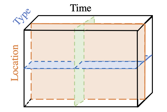
(a) An example of tensor time series, which is comprised of three modes: location, data type and time.

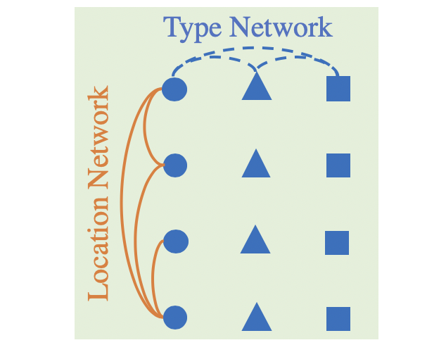
(b) A temporal snapshot. Rows and columns present locations and data types, which are constrained by their networks.

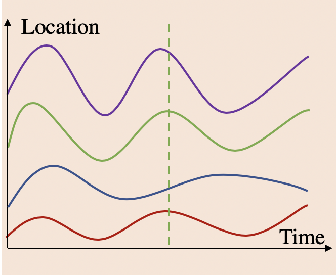
(c) A slice along one data type: co-evolving time series of the same data type at different locations.

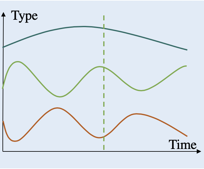
(d) A slice along one location: co-evolving time series of different data types at the same location.

Figure 1. An exemplary tensor time series and three slices along different dimensions. (Best viewed in color.)

Co-evolving time series naturally arises in numerous applications, ranging from environmental monitoring (Banzon et al., 2016; Srivastava and Lessmann, 2018), financial analysis (Tsay, 2014) to smart transportation (Li et al., 2017; Yu et al., 2017b; Li et al., 2019). As shown in Figure 1(a) and 1(b), each temporal snapshot of the co-evolving time series naturally forms a multi-dimensional array, i.e., a multi-mode tensor (Rogers et al., 2013). For example, the spatial-temporal monitoring data of atmosphere is a time series of an $N_{1}\times N_{2}\times N_{3}\times N_{4}$ tensor, where $N_{1}$, $N_{2}$, $N_{3}$ and $N_{4}$ denote latitude, longitude, elevation and air conditions respectively (e.g. temperature, pressure and oxygen concentration). Companies’ financial data is a time series of an $N_{1}\times N_{2}\times N_{3}$ tensor, where $N_{1}$, $N_{2}$ and $N_{3}$ denote the companies, the types of financial data (e.g. revenue, expenditure) and the statistics of them respectively. Nonetheless, the vast majority of the recent deep learning methods for co-evolving time series (Li et al., 2017; Yu et al., 2017b; Li et al., 2019; Yan et al., 2018; Liang et al., 2018) have almost exclusively focused on a single mode.

Data points within a tensor are usually related to each other, and different modes are associated with different relationships (Figure 1(b)). Within the above example of environmental monitoring, along geospatial modes ($N_{1}$, $N_{2}$ and $N_{3}$), we could know the (latitudinal, longitudinal and elevational) location relationship between two data points. In addition, different data types ($N_{4}$) are also related with each other. As governed by Gay-Lussac’s law (Barnett, 1941), given fixed mass and volume, the pressure of a gas is proportional to the Kelvin temperature. These relationships can be explicitly modeled by networks or graphs (Chakrabarti and Faloutsos, 2006; Akoglu et al., 2015). Compared with the rich machinery of deep graph convolutional methods for flat graphs (Kipf and Welling, 2016; Defferrard et al., 2016), multiple graphs associated with a tensor (referred to as tensor graphs in this paper) are less studied. To fill this gap, we propose a novel Tensor Graph Convolution Network (TGCN) which extends Graph Convolutional Network (GCN) (Kipf and Welling, 2016) to tensor graphs based on multi-dimensional convolution.

Another key challenge for modeling the temporal dynamics behind co-evolving time series is how to capture the implicit relationship of different time series. As shown in Figure 1(c), the temporal patterns of time series with the same data type (e.g. temperature) are similar. The relationship of the co-evolving temperature time series can be partially captured by the location network, e.g., two neighboring locations often have similar temporal dynamics. However, the temperature time series from two locations far apart could also share similar patterns. Most of the existing studies either use the same temporal model for all time series (Li et al., 2017; Yu et al., 2017b; Li et al., 2019; Yan et al., 2018), or use separate Recurrent Neural Networks (RNN) (Srivastava and Lessmann, 2018; Zhou and Huang, 2017) for different time series. Nonetheless, none of them offers a principled way to model the implicit relationship. To tackle with this challenge, we propose a novel Tensor Recurrent Neural Network (TRNN) based on Multi-Linear Dynamic System (MLDS) (Rogers et al., 2013) and Tucker decomposition, which helps reduce the number of model parameters.

Our main contributions are summarized as follows:

• We introduce a novel graph convolution for tensor graphs and present a novel TGCN that generalizes GCN (Kipf and Welling, 2016). The new architecture can capture the synergy among different graphs by simultaneously performing convolution on them.

• We introduce a novel TRNN based on MLDS (Rogers et al., 2013) for efficiently modeling the implicit relationship between complex temporal dynamics of tensor time series.

• We present comprehensive evaluations for the proposed methods on a variety of real-world datasets to demonstrate the effectiveness of the proposed method.

The rest of the paper is organized as follows. In Section 2, we briefly introduce relevant definitions about graph convolution and tensor algebra, and formally introduce the definition of network of tensor time series. In Section 3, we present and analyze the proposed TGCN and TRNN. The experimental results are presented in Section 4. Related works and conclusion are presented in Section 5 and Section 6 respectively.

2. Preliminaries

In this section, we formally define network of tensor time series (Subsection 2.3), after we review the preliminaries, including graph convolution on flat graphs (Subsection 2.1), tensor algebra (Subsection 2.2), and multi-dimensional Fourier transformation (Subsection 2.3) respectively. We introduce the definitions of the problems in Section 2.5.

2.1. Graph Convolution on Flat Graphs

Analogous to the one-dimensional Discrete Fourier Transform (Definition 2.2), the graph Fourier transform is given by Definition 2.3. Then the spectral graph convolution (Definition 2.4) is defined based on one-dimensional convolution and the convolution theorem. The free parameter of the convolution filter is further replaced by Chebyshev polynomials and thus we have Chebyshev approximation for graph convolution (Definition 2.5).

Definition 2.1 (Flat Graph).

A flat graph contains a one-dimentional graph signal $\mathbf{x}\in\mathbb{R}^{N}$ and an adjacency matrix $\mathbf{A}\in\mathbb{R}^{N\times N}$.

Definition 2.2 (Discrete Fourier Transform).

Given an one dimensional signal $\mathbf{x}\in\mathbb{R}^{N}$, where $N$ is the length of the sequence, its Fourier transform is defined by:

(1) $$\tilde{\mathbf{x}}[n]=\sum_{k=1}^{N}\mathbf{x}[k]e^{-\frac{i2\pi}{N}kn}$$

where $\mathbf{x}[k]$ is the $k$-th element of $\mathbf{x}$ and $\tilde{\mathbf{x}}[n]$ is the $n$-th element of the transformed vector $\tilde{\mathbf{x}}$. The above definition can be rewritten as:

(2) $$\tilde{\mathbf{x}}=\mathbf{F}\mathbf{x}$$

where $\mathbf{F}\in\mathbb{R}^{N\times N}$ is the filter matrix and $\mathbf{F}[n,k]=e^{-\frac{i2\pi}{N}kn}$.

Definition 2.3 (Graph Fourier Transform (Bruna et al., 2013)).

Given a graph signal $\mathbf{x}\in\mathbb{R}^{N}$, along with its adjacency matrix $\mathbf{A}\in\mathbb{R}^{N\times N}$, where $N$ is the number of nodes, the graph Fourier transform is defined by:

(3) $$\tilde{\mathbf{x}}=\mathbf{\Phi}^{T}\mathbf{x}$$

where $\mathbf{\Phi}$ is the eigenvector matrix of the graph Laplacian matrix $\mathbf{L}=\mathbf{I}-\mathbf{D}^{-\frac{1}{2}}\mathbf{A}\mathbf{D}^{-\frac{1}{2}}=\mathbf{\Phi}\mathbf{\Lambda}\mathbf{\Phi}^{T}$, $\mathbf{I}\in\mathbb{R}^{N\times N}$, $\mathbf{D}\in\mathbb{R}^{N\times N}$ denote the identity matrix and the degree matrix, and $\mathbf{\Lambda}$ is a diagonal matrix whose diagonal elements are eigenvalues.

Definition 2.4 (Spectral Graph Convolution (Bruna et al., 2013)).

Given a signal $\mathbf{x}\in\mathbb{R}^{N}$ and a filter $\mathbf{g}\in\mathbb{R}^{N}$, the spectral graph convolution is defined in the Fourier domain according to the convolution theorem:

(4) $$\mathbf{\Phi}^{T}(\mathbf{g}\star\mathbf{x}) =(\mathbf{\Phi}^{T}\mathbf{g})\odot(\mathbf{\Phi}^{T}\mathbf{x})$$

(5) $$\mathbf{g}\star\mathbf{x} =\mathbf{\Phi}(\mathbf{\Phi}^{T}\mathbf{g})\odot(\mathbf{\Phi}^{T}\mathbf{x})=\mathbf{\Phi}\text{diag}(\tilde{\mathbf{g}})\mathbf{\Phi}^{T}\mathbf{x}$$

where $\star$ and $\odot$ denote convolution operation and Hadamard product; the second equation holds due to the orthonormality.

Definition 2.5 (Chebyshev Approximation for Spectral Graph Convolution (Defferrard et al., 2016)).

Given an input graph signal $\mathbf{x}\in\mathbb{R}^{N}$ and its adjacency matrix $\mathbf{A}\in\mathbb{R}^{N\times N}$, the Chebyshev approximation for graph convolution on a flat graph is given by (Kipf and Welling, 2016; Defferrard et al., 2016):

(6) $$\mathbf{g}_{\theta}\star\mathbf{x}=\mathbf{\Phi}(\sum_{p=0}^{P}\theta_{p}T_{p}(\tilde{\mathbf{\Lambda}}))\mathbf{\Phi}^{T}\mathbf{x}=\sum_{p=0}^{P}\theta_{p}T_{p}(\tilde{\mathbf{L}})\mathbf{x}$$

where $\tilde{\mathbf{\Lambda}}=\frac{2}{\lambda_{max}}\mathbf{\Lambda}-\mathbf{I}$ is the normalized eigenvalues, $\lambda_{max}$ is maximum eigenvalue of the matrix $\mathbf{\Lambda}$; $\tilde{\mathbf{L}}=\frac{2}{\lambda_{max}}\mathbf{L}-\mathbf{I}$; $T_{p}(x)$ is Chebyshev polynomials defined by $T_{p}(x)=2xT_{p-1}(x)-T_{p-2}(x)$ with $T_{0}(x)=1$ and $T_{1}(x)=x$, and $p$ denotes the order of polynomials; $\mathbf{g}_{\theta}$ and $\theta_{p}$ denote the filter vector and the parameter respectively.

2.2. Tensor Algebra

Definition 2.6 (Mode-m Product).

The mode-m product generalizes matrix-matrix product to tensor-matrix product. Given a matrix $\mathbf{U}\in\mathbb{R}^{N_{m}\times N^{\prime}}$, and a tensor $\mathcal{X}\in\mathbb{R}^{N_{1}\times\cdots N_{m-1}\times N_{m}\times N_{m+1}\cdots\times N_{M}}$, then $\mathcal{X}\times_{m}\mathbf{U}\in\mathbb{R}^{N_{1}\times\cdots N_{m-1}\times N^{\prime}\times N_{m+1}\cdots\times N_{M}}$ is its mode-m product. Its element $[n_{1},\cdots,n_{m-1},n^{\prime},n_{m+1},\cdots,n_{M}]$ is defined as:

(7) $$\begin{split}&(\mathcal{X}\times_{m}\mathbf{U})[n_{1},\cdots,n_{m-1},n^{\prime},n_{m+1},\cdots,n_{M}]\\ =&\sum_{n_{m}=1}^{N_{m}}\mathcal{X}[n_{1},\cdots,n_{m-1},n_{m},n_{m+1},\cdots,n_{M}]\mathbf{U}[n_{m},n^{\prime}]\end{split}$$

Definition 2.7 (Tucker Decomposition).

The Tucker decomposition can be viewed as a form of high-order principal component analysis (Kolda and Bader, 2009). A tensor $\mathcal{X}\in\mathbb{R}^{N_{1}\times\cdots\times N_{M}}$ can be decomposed into a smaller core tensor $\mathcal{Z}\in\mathbb{R}^{N^{\prime}_{1}\times\cdots\times N^{\prime}_{M}}$ by $M$ orthonormal matrices $\mathbf{U}_{m}\in\mathbb{R}^{N^{\prime}_{m}\times N_{m}}$ ($N^{\prime}_{m}<N_{m}$):

(8) $$\mathcal{X}=\mathcal{Z}\prod_{m=1}^{M}\times_{m}\mathbf{U}_{m}$$

The matrix $\mathbf{U}_{m}$ is comprised of principal components for the $m$-th mode and the core tensor $\mathcal{Z}$ indicates the interactions among the components. Due to the orthonormality of $\mathbf{U}_{m}$, we have:

(9) $$\mathcal{Z}=\mathcal{X}\prod_{m=1}^{M}\times_{m}\mathbf{U}_{m}^{T}$$

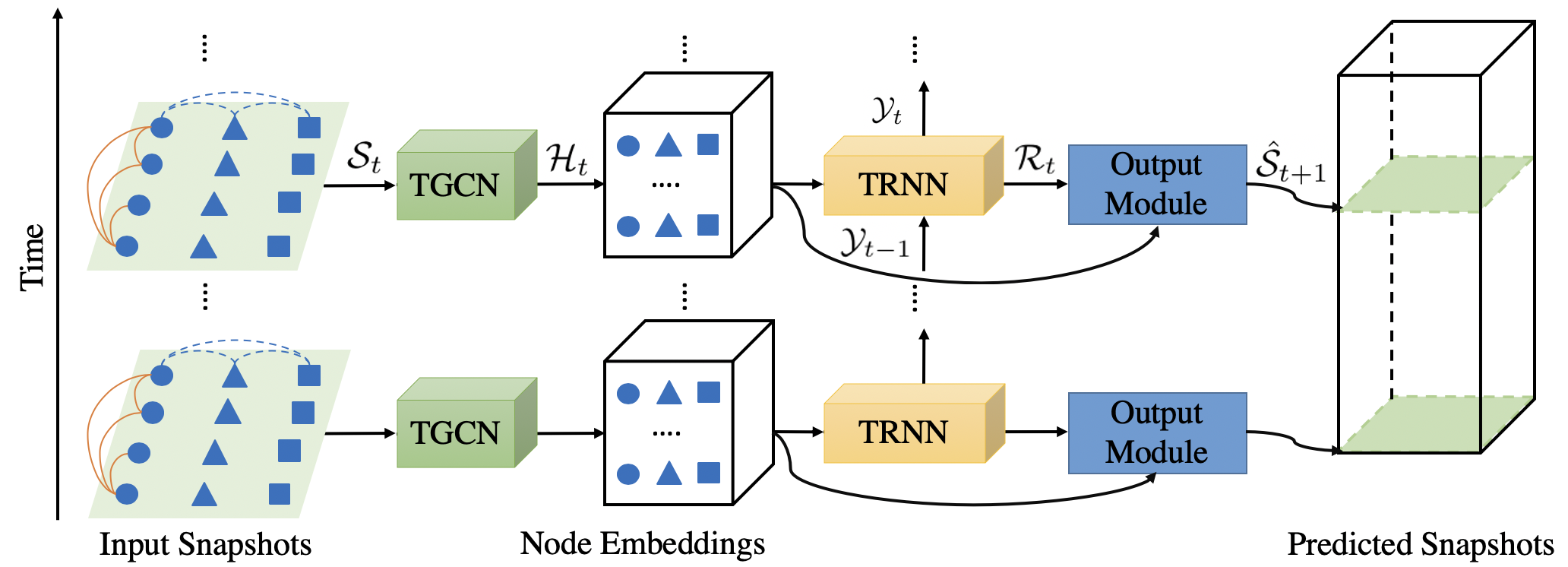
Figure 2. The framework of the proposed model NeT³. At each time step $t$, the model takes a snapshot $\mathcal{S}_{t}$ from the tensor time series $\mathcal{S}$ and extracts its node embedding tensor $\mathcal{H}_{t}$ via Tensor Graph Convolution Network (TGCN) module. $\mathcal{H}_{t}$ will be fed into the Tensor RNN (TRNN) module to encode the temporal dynamics. Finally, the output module takes both of $\mathcal{H}_{t}$ and $\mathcal{R}_{t}$ to predict the snapshot of the next time step $\hat{\mathcal{S}}_{t+1}$. Note that $\mathcal{Y}_{t}$ and $\mathcal{Y}_{t+1}$ are the hidden states of TRNN at time step $t$ and $t+1$ respectively.

2.3. Multi-dimensional Fourier Transform

Definition 2.8 (Multi-dimensional Discrete Fourier Transform).

Given a multi-dimensional/mode signal $\mathcal{X}\in\mathbb{R}^{N_{1}\times\cdots\times N_{M}}$, the multi-dimensional Fourier transform is defined by:

(10) $$\begin{split}\tilde{\mathcal{X}}[n_{1},\cdots,n_{M}]=\prod_{m=1}^{M}\sum_{k_{m}=1}^{N_{m}}e^{-\frac{i2\pi}{N_{m}}k_{m}n_{m}}\mathcal{X}[k_{1},\cdots,k_{M}]\end{split}$$

Similar to the one-dimensional Fourier transform (Definition 2.2), the above equation can be re-written by a multi-linear form:

(11) $$\tilde{\mathcal{X}}=\mathcal{X}\times_{1}\mathbf{F_{1}}\cdots\times_{M}\mathbf{F_{M}}=\mathcal{X}\prod_{m=1}^{M}\times_{m}\mathbf{F}_{m}$$

where $\times_{m}$ denotes the mode-m product, $\mathbf{F}_{m}\in\mathbb{R}^{N_{m}\times N_{m}}$ is the filter matrix, and $\mathbf{F}_{m}[n,k]=e^{-\frac{i2\pi}{N_{m}}kn}$.

Definition 2.9 (Separable Multi-dimensional Convolution).

The separable multi-dimensional convolution is defined based on Definition 2.8. Given a signal $\mathcal{X}\in\mathbb{R}^{N_{1}\times\cdots\times N_{M}}$ and a separable filter $\mathcal{Y}\in\mathbb{R}^{N_{1}\times\cdots\times N_{M}}$ such that $\mathcal{Y}[n_{1},\cdots,n_{m}]=\mathbf{y}_{1}[n_{1}]\cdots\mathbf{y}_{M}[n_{m}]$, where $\mathbf{y}_{m}\in\mathbb{R}^{N_{m}}$ is the filter vector for the $m$-th mode, then the multi-dimensional convolution is the same as iteratively applying one dimensional convolution onto $\mathcal{X}$:

(12) $$\begin{split}\mathcal{Y}\star\mathcal{X}=\mathbf{y}_{1}\star_{1}\cdots\star_{M-1}\mathbf{y}_{M}\star_{M}\mathcal{X}\end{split}$$

where $\star_{m}$ denotes convolution on the $m$-th mode.

Suppose $\mathcal{X}\in\mathbb{R}^{N_{1}\times N_{2}}$ and $\mathcal{Y}=\mathbf{y}_{1}\cdot\mathbf{y}_{2}^{T}$, where $\mathbf{y}_{1}\in\mathbb{R}^{N_{1}}$ and $\mathbf{y}_{2}\in\mathbb{R}^{N_{2}}$. Then $\mathcal{Y}\star\mathcal{X}$ means applying $\mathbf{y}_{1}$ and $\mathbf{y}_{2}$ to the rows and columns of $\mathcal{X}$ respectively. Formally we have:

(13) $$\mathcal{Y}\star\mathcal{X}=\mathbf{y}_{1}\star_{1}\mathbf{y}_{2}\star_{2}\mathcal{X}=\mathbf{Y}_{1}^{T}\mathcal{X}\mathbf{Y}_{2}=\mathcal{X}\prod_{m=1}^{2}\times_{m}\mathbf{Y}_{m}$$

where $\mathbf{Y}_{1}\in\mathbb{R}^{N_{1}\times N_{1}}$ and $\mathbf{Y}_{2}\in\mathbb{R}^{N_{2}\times N_{2}}$ are the transformation matrix corresponding to $\mathbf{y}_{1}$ and $\mathbf{y}_{2}$ respectively.

2.4. Network of Tensor Time Series

Definition 2.10 (Tensor Time Series).

A tensor time series is a $(M+1)$-mode tensor $\mathcal{S}\in\mathbb{R}^{N_{1}\times\cdots\times N_{M}\times T}$ or $\{\mathcal{S}_{t}\in\mathbb{R}^{N_{1}\times\cdots\times N_{M}}\}_{t=1}^{T}$, where the $(M+1)$-th mode is the time and its dimension is $T$.

Definition 2.11 (Tensor Graph).

The tensor graph is comprised of a $M$-mode tensor $\mathcal{X}\in\mathbb{R}^{N_{1}\times\cdots\times N_{M}}$ and the adjacency matrices for each mode $\mathbf{A}_{m}\in\mathbb{R}^{N_{m}\times N_{m}}$. Note that if $m$-th mode is not associated with an adjacency matrix, then $\mathbf{A}_{m}=\mathbf{I}_{m}$, where $\mathbf{I}_{m}\in\mathbb{R}^{N_{m}\times N_{m}}$ denotes the identity matrix.

Definition 2.12 (Network of Tensor Time Series).

A network of tensor time series is comprised of (1) a tensor time series $\mathcal{S}\in\mathbb{R}^{N_{1}\times\cdots\times N_{M}\times T}$ and (2) a set of adjacency matrices $\mathbf{A}_{m}\in\mathbb{R}^{N_{m}\times N_{m}}$ ($m\in[1,\cdots,M]$) for all but the last mode (i.e., the time mode).

2.5. Problem Definition

In this paper, we focus on the representation learning for the network of tensor time series by predicting its future values. The model trained by predicting the future values can also be applied to recover the missing values of the time series.

Definition 2.13 (Future Value Prediction).

Given a network of tensor time series with $\mathcal{S}\in\mathbb{R}^{N_{1}\times\cdots\times N_{M}\times T}$ and $\{\mathbf{A}_{m}\in\mathbb{R}^{N_{m}\times N_{m}}\}_{m=1}^{M}$, and a time step $T^{\prime}$, the task of the future value prediction is to predict the future values of $\mathcal{S}$ from $T+1$ to $T+T^{\prime}$.

Definition 2.14 (Missing Value Recovery).

We formulate the task of missing value recovery from the perspective of future value prediction. Suppose the data point $\mathcal{S}[n_{1},\cdots,n_{M},T^{\prime}]$ ($T^{\prime}\leq T$) of $\mathcal{S}\in\mathbb{R}^{N_{1}\times\cdots\times N_{M}\times T}$ is missing, then we takes $\omega\leq T^{\prime}$ historical values of $\mathcal{S}$ prior to the time step $T^{\prime}$: $\{\mathcal{S}_{t}\}_{\omega=T^{\prime}-\omega}^{T^{\prime}-1}$ as input, and predict the value of the $\hat{\mathcal{S}}[n_{1},\cdots,n_{M},T^{\prime}]$.

3. Methodology

An overview of the proposed NeT³ is presented in Figure 2, which works as follows. At each time step $t$, the proposed Tensor Graph Convolutional Network (TGCN) (Section 3.1) takes as input the $t$-th snapshot $\mathcal{S}_{t}\in\mathbb{R}^{N_{1}\times\cdots\times N_{M}}$ along with its adjacency matrices $\{\mathbf{A}_{m}\in\mathbb{R}^{N_{m}\times N_{m}}\}_{m=1}^{M}$ and extracts its node embedding tensor $\mathcal{H}_{t}$, which will be fed into the proposed Tensor Recurrent Neural Network (TRNN) (Section 3.2) to encode temporal dynamics and produce $\mathcal{R}_{t}$. Finally, the output module (Section 3.3) takes both $\mathcal{H}_{t}$ and $\mathcal{R}_{t}$ to predict the snapshot of the next time step $\hat{\mathcal{S}}_{t+1}$. Note that $\mathcal{Y}_{t}$ in Figure 2 denotes the hidden state of TRNN at the time step $t$.

3.1. Tensor Graph Convolution Network

In this subsection, we first introduce spectral graph convolution on tensor graphs and its Chebychev approximation in Subsection 3.1.1. Then we provide a detailed derivation for the layer-wise updating function of the proposed TGCN in Subsection 3.1.2.

3.1.1. Spectral Convolution for Tensor Graph

Analogues to the multi-dimensional Fourier transform (Definition 2.8) and the graph Fourier transform on flat graphs (Definition 2.3), we first define the Fourier transform on tensor graphs in Definition 3.1. Then based on the separable multi-dimensional convolution (Definition 2.9), and tensor graph Fourier transform (Definition 3.1), we propose spectral convolution on tensor graphs in Definition 3.2. Finally, in Definition 3.3, we propose to use Chebychev approximation in order to parameterize the free parameters in the filters of spectral convolution.

Definition 3.1 (Tensor Graph Fourier Transform).

Given a graph signal $\mathcal{X}\in\mathbb{R}^{N_{1}\times\cdots\times N_{M}}$, along with its adjacency matrices for each mode $\mathbf{A}_{m}\in\mathbb{R}^{N_{m}\times N_{m}}$ ($m\in[1,\cdots,M]$), the tensor graph Fourier transform is defined by:

(14) $$\tilde{\mathcal{X}}=\mathcal{X}\prod_{m=1}^{M}\times_{m}\mathbf{\Phi}_{m}$$

where $\mathbf{\Phi}_{m}$ is the eigenvector matrix of graph Laplacian matrix $\mathbf{L}_{m}=\mathbf{\Phi}_{m}\mathbf{\Lambda}_{m}\mathbf{\Phi}_{m}^{T}$ for $\mathbf{A}_{m}$; $\times_{m}$ denotes the mode-m product.

Definition 3.2 (Spectral Convolution for Tensor Graph).

Given an input graph signal $\mathcal{X}\in\mathbb{R}^{N_{1}\times\cdots\times N_{M}}$, and a multi-dimensional filter $\mathcal{G}\in\mathbb{R}^{N_{1}\times\cdots\times N_{M}}$ defined by $\mathcal{G}[n_{1},\cdots,n_{M}]=\mathbf{g}_{1}[n_{1}]\cdots\mathbf{g}_{M}[n_{M}]$, where $\mathbf{g}_{m}\in\mathbb{R}^{N_{m}}$ is the filter vector for the $m$-th mode. By analogizing to spectral graph convolution (Definition 2.4) and separable multi-dimensional convolution (Definition 2.9) , we define spectral convolution for tensor graph as:

(15) $$\mathcal{G}\star\mathcal{X}=\mathcal{X}\prod_{m=1}^{M}\times_{m}\mathbf{\Phi}^{T}_{m}\textrm{diag}(\tilde{\mathbf{g}}_{m})\mathbf{\Phi}_{m}$$

where $\tilde{\mathbf{g}}_{m}=\mathbf{\Phi}_{m}^{T}\mathbf{g}_{m}$ is the Fourier transformed filter for the $m$-th mode; $\star$ and $\times_{m}$ denote the convolution operation and the mode-m product respectively; $\textrm{diag}(\mathbf{g}_{m})$ denotes the diagonal matrix, of which the diagonal elements are the elements in $\mathbf{g}_{m}$.

Definition 3.3 (Chebyshev Approximation for Spectral Convolution on Tensor Graph).

Given a tensor graph $\mathcal{X}\in\mathbb{R}^{N_{1}\times\cdots\times N_{M}}$, where each mode is associated with an adjacency matrix $\mathbf{A}_{m}\in\mathbb{R}^{N_{m}\times N_{m}}$, the Chebychev approximation for spectral convolution on tensor graphs is given by approximating $\tilde{\mathbf{g}}_{m}$ by Chebyshev polynomials:

(16) $$\begin{split}\mathcal{G}_{\theta}\star\mathcal{X}&=\mathcal{X}\prod_{m=1}^{M}\times_{m}\mathbf{\Phi}^{T}_{m}(\sum_{p_{m}=0}^{P}\theta_{m,p_{m}}T_{p_{m}}(\tilde{\mathbf{\Lambda}}_{m}))\mathbf{\Phi}_{m}\\ &=\mathcal{X}\prod_{m=1}^{M}\times_{m}\sum_{p_{m}=0}^{P}\theta_{m,p_{m}}T_{p_{m}}(\tilde{\mathbf{L}}_{m})\end{split}$$

where $\mathcal{G}_{\theta}$ denotes the convolution filter parameterized by $\theta$; $\mathbf{\Lambda}_{m}\in\mathbb{R}^{N_{m}\times N_{m}}$ is the matrix of eigenvalues for the graph Laplacian matrix $\mathbf{L}_{m}=\mathbf{I}_{m}-\mathbf{D}_{m}^{-\frac{1}{2}}\mathbf{A}_{m}\mathbf{D}_{m}^{-\frac{1}{2}}=\mathbf{\Phi}_{m}\mathbf{\Lambda}_{m}\mathbf{\Phi}_{m}^{T}$; $\tilde{\mathbf{\Lambda}}_{m}=\frac{2}{\lambda_{m,max}}\mathbf{\Lambda}_{m}-\mathbf{I}_{m}$ is the normalized eigenvalues, $\lambda_{m,max}$ is maximum eigenvalue in the matrix $\mathbf{\Lambda}_{m}$; $\tilde{\mathbf{L}}_{m}=\frac{2}{\lambda_{m,max}}\mathbf{L}_{m}-\mathbf{I}_{m}$; $T_{p_{m}}(x)$ is Chebyshev polynomials defined by $T_{p_{m}}(x)=2xT_{p_{m}-1}(x)-T_{p_{m}-2}(x)$ with $T_{0}(x)=1$ and $T_{1}(x)=x$, and $p_{m}$ denotes the order of polynomials; $\theta_{m,p_{m}}$ denote the co-efficient of $T_{p_{m}}(x)$. For clarity, we use the same polynomial degree $P$ for all modes.

3.1.2. Tensor Graph Convolutional Layer

Due to the linearity of mode-m product, Equation (16) can be re-formulated as:

(17) $$\begin{split}\mathcal{G}_{\theta}\star\mathcal{X}&=\sum_{p_{1},\cdots,p_{M}=0}^{P}\mathcal{X}\prod_{m=1}^{M}\times_{m}\theta_{m,p_{m}}T_{p_{m}}(\tilde{\mathbf{L}}_{m})\\ &=\sum_{p_{1},\cdots,p_{M}=0}^{P}\prod_{m=1}^{M}\theta_{m,p_{m}}\mathcal{X}\prod_{m=1}^{M}\times_{m}T_{p_{m}}(\tilde{\mathbf{L}}_{m})\end{split}$$

We follow (Kipf and Welling, 2016) to simplify Equation (17). Firstly, let $\lambda_{m,max}=2$ and we have:

(18) $$\begin{split}\tilde{\mathbf{L}}_{m}&=\frac{2}{\lambda_{m,max}}\mathbf{L}_{m}-\mathbf{I}_{m}\\ &=\mathbf{I}_{m}-\mathbf{D}_{m}^{-\frac{1}{2}}\mathbf{A}_{m}\mathbf{D}_{m}^{-\frac{1}{2}}-\mathbf{I}_{m}\\ &=-\mathbf{D}_{m}^{-\frac{1}{2}}\mathbf{A}_{m}\mathbf{D}_{m}^{-\frac{1}{2}}\end{split}$$

For clarity, we use $\tilde{\mathbf{A}}_{m}$ to represent $\mathbf{D}_{m}^{-\frac{1}{2}}\mathbf{A}_{m}\mathbf{D}_{m}^{-\frac{1}{2}}$. Then we fix $P=1$ and drop the negative sign in Equation (18) by absorbing it to parameter $\theta_{m,p_{m}}$. Therefore, we have

(19) $$\sum_{p=0}^{P}\theta_{m,p_{m}}T_{p}(\tilde{\mathbf{L}}_{m})=\theta_{m,0}+\theta_{m,1}\tilde{\mathbf{A}}_{m}$$

Furthermore, by plugging Equation (19) back into Equation (17) and replacing the product of parameters $\prod_{m=1}^{M}\theta_{m,p_{m}}$ by a single parameter $\theta_{p_{1},\cdots,p_{M}}$, we will obtain:

(20) $$\begin{split}\mathcal{G}_{\theta}\star\mathcal{X}=\sum_{\exists p_{m}=1}\theta_{p_{1},\cdots,p_{M}}\mathcal{X}\prod_{p_{m}=1}\times_{m}\tilde{\mathbf{A}}_{m}+\theta_{0,\cdots,0}\mathcal{X}\end{split}$$

We can observe from the above equation that $p_{m}$ works as an indicator for whether applying the convolution filter $\tilde{\mathbf{A}}_{m}$ to $\mathcal{X}$ or not. If $p_{m}=1$, then $\tilde{\mathbf{A}}_{m}$ will be applied to $\mathcal{X}$, otherwise, $\mathbf{I}_{m}$ will be applied. When $p_{m}=0$ for $\forall m\in[1,\cdots,M]$, we will have $\theta_{0,\cdots,0}\mathcal{X}$. To better understand how the above approximation works on tensor graphs, let us assume $M=2$. Then we have:

(21) $$\mathcal{G}_{\theta}\star\mathcal{X}=\theta_{1,1}\mathcal{X}\times_{1}\tilde{\mathbf{A}}_{1}\times_{2}\tilde{\mathbf{A}}_{2}+\theta_{1,0}\mathcal{X}\times_{1}\tilde{\mathbf{A}}_{1}+\theta_{0,1}\mathcal{X}\times_{2}\tilde{\mathbf{A}}_{2}+\theta_{0,0}\mathcal{X}$$

Given the approximation in Equation (20), we propose the tensor graph convolution layer in Definition 3.4.

Definition 3.4 (Tensor Graph Convolution Layer).

Given an input tensor $\mathcal{X}\in\mathbb{R}^{N_{1}\times\cdots\times N_{M}\times d}$, where $d$ is the number of channels, along with its adjacency matrices $\{\mathbf{A}_{m}\}_{m=1}^{M}$, the Tensor Graph Convolution Layer (TGCL) with $d^{\prime}$ output channels is defined by:

(22) $$\begin{split}&\text{TGCL}(\mathcal{X},\{\mathbf{A}_{m}\}_{m=1}^{M})\\ =&\sigma(\sum_{\exists p_{m}=1}\mathcal{X}\prod_{p_{m}=1}\times_{m}\tilde{\mathbf{A}}_{m}\times_{M+1}\mathbf{\Theta}_{p_{1},\cdots,p_{M}}+\mathcal{X}\times_{M+1}\mathbf{\Theta}_{0})\end{split}$$

where $\mathbf{\Theta}\in\mathbb{R}^{d\times d^{\prime}}$ is parameter matrix; $\sigma(\cdot)$ is activation function.

In the NeT³model (Figure 2), given a snapshot $\mathcal{S}_{t}\in\mathbb{R}^{N_{1}\times\cdots\times N_{M}}$ along with its adjacency matrices $\{\mathbf{A}_{m}\}_{m=1}^{M}$, we use a one layer TGCL to obtain the node embeddings $\mathcal{H}_{t}\in\mathbb{R}^{N_{1}\times\cdots\times N_{M}\times d}$, where $d$ is the dimension of the node embeddings:

(23) $$\mathcal{H}_{t}=\textrm{TGCN}(\mathcal{S}_{t})$$

3.1.3. Synergy Analysis

The proposed TGCL effectively models tensor graphs and captures the synergy among different adjacency matrices. The vector $\mathbf{p}=[p_{1},\cdots,p_{M}]\in[0,1]^{M}$ represents a combination of $M$ networks, where $p_{m}=1$ and $p_{m}=0$ respectively indicate the presence and absence of the $\tilde{\mathbf{A}}_{m}$. Therefore, each node in $\mathcal{X}$ could collect other nodes’ information along the adjacency matrix $\tilde{\mathbf{A}}_{m}$ if $p_{m}=1$. For example, suppose $M=2$ and $p_{1}=p_{2}=1$ (as shown in Figure 3 and Equation (21)), then node $\mathcal{X}[1,1]$ (node $v$) could reach node $\mathcal{X}[2,2]$ (node $w^{\prime}$) by passing node $\mathcal{X}[2,1]$ along the adjacency matrix $\tilde{\mathbf{A}}_{1}$ ($\mathcal{X}\times_{1}\tilde{\mathbf{A}}_{1}$) and then arriving at node $\mathcal{X}[2,2]$ via $\tilde{\mathbf{A}}_{2}$ ($\mathcal{X}\times_{1}\tilde{\mathbf{A}}_{1}\times_{2}\tilde{\mathbf{A}}_{2}$). In contrast, with a traditional GCN layer, node $v$ can only gather information of its direct neighbors from a given model (node $v^{\prime}$ via $\tilde{\mathbf{A}}_{1}$ or $w$ via $\tilde{\mathbf{A}}_{2}$).

An additional advantage of TGCL lies in that it is robust to missing values in $\mathcal{X}$ since TGCL is able to recover the value of a node from various combination of adjacency matrices. For example, suppose the value of node $v=0$, then TGCL could recover its value by referencing the value of $v^{\prime}$ (via $\mathcal{X}\times_{1}\tilde{\mathbf{A}}_{1}$), or the value of $w$ (via $\mathcal{X}\times_{2}\tilde{\mathbf{A}}_{2}$), or the value of $w^{\prime}$ (via $\mathcal{X}\times_{1}\tilde{\mathbf{A}}_{1}\times_{2}\tilde{\mathbf{A}}_{2}$). However, a GCN layer could only refer to the node $v^{\prime}$ via $\tilde{\mathbf{A}}_{1}$ or $w$ via $\tilde{\mathbf{A}}_{2}$.

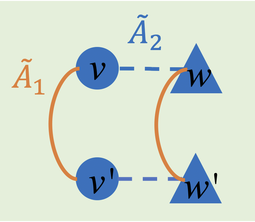
Figure 3. An illustration of synergy analysis of TGCL.

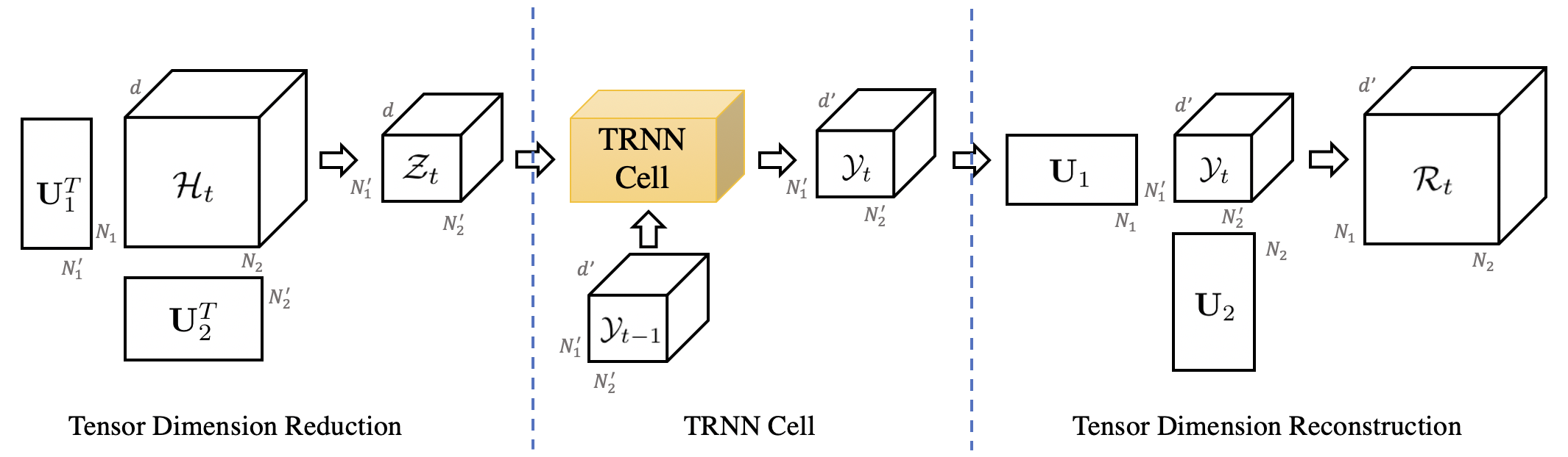
Figure 4. Tensor Recurrent Neural Network (TRNN).

3.1.4. Complexity Analysis

For a $M$-mode tensor with $K(1\leq K\leq M)$ networks, the complexity of the tensor graph convolution (Equation (20)) is $O(2^{K-1}\prod_{m=1}^{M}N_{m}(2+\sum_{k=1}^{K}N_{k}))$.

3.2. Tensor Recurrent Neural Network

Given the output from TGCN: $\mathcal{H}_{t}\in\mathbb{R}^{N_{1}\times\cdots\times N_{M}\times d}$ (Equation (23)), the next step is to incorporate temporal dynamics for $\mathcal{H}_{t}$.

As shown in Figure 4, we propose a novel Tensor Recurrent Neural Network (TRNN), which captures the implicit relation among co-evolving time series by decomposing $\mathcal{H}_{t}$ into a low dimensional core tensor $\mathcal{Z}_{t}\in\mathbb{R}^{N_{1}^{\prime}\times\cdots\times N_{M}^{\prime}\times d}$ ($N_{m}^{\prime}<N_{m}$) via a Tensor Dimension Reduction module (Section 3.2.1). The Tensor RNN Cell (Section 3.2.2) further introduces non-linear temporal dynamics into $\mathcal{Z}_{t}$ and produces the hidden state $\mathcal{Y}_{t}\in\mathbb{R}^{N_{1}^{\prime}\times\cdots\times N_{M}^{\prime}\times d}$. Finally, the Tensor Dimension Reconstruction module (Section 3.2.3) reconstructs $\mathcal{Y}_{t}$ and generates the reconstructed tensor $\mathcal{R}_{t}\in\mathbb{R}^{N_{1}\times\cdots\times N_{M}\times d}$.

3.2.1. Tensor Dimension Reduction

As shown in the left part of Figure 4, the proposed tensor dimension reduction module will reduce the dimensionality of each mode of $\mathcal{H}_{t}\in\mathbb{R}^{N_{1}\times\cdots\times N_{M}\times d}$, except for the last mode (hidden features), by leveraging Tucker decomposition (Definition 2.7):

(24) $$\mathcal{Z}_{t}=\mathcal{H}_{t}\prod_{m=1}^{M}\times_{m}\mathbf{U}_{m}^{T}$$

where $\mathbf{U}_{m}\in\mathbb{R}^{N^{\prime}_{m}\times N_{m}}$ denotes the orthonormal parameter matrix, which is learnable via backpropagation; $\mathcal{Z}_{t}\in\mathbb{R}^{N_{1}^{\prime}\times\cdots\times N_{m}^{\prime}\times d}$ is the core tensor of $\mathcal{H}_{t}$.

3.2.2. Tensor RNN Cell

Classic RNN cells, e.g. Long-Short-Term-Memory (LSTM) (Hochreiter and Schmidhuber, 1997) are designed for a single input sequence, and therefore do not directly capture the correlation among co-evolving sequences. To address this problem, we propose a novel Tensor RNN (TRNN) cell based on tensor algebra.

We first propose a Tensor Linear Layer (TLL):

(25) $$\text{TLL}(\mathcal{X})=\mathcal{X}\prod_{m=1}^{M+1}\times_{m}\mathbf{W}_{m}+\mathbf{b}$$

where $\mathcal{X}\in\mathbb{R}^{N_{1}\times\cdots\times N_{M}\times d}$ is the input tensor, and $\mathbf{W}_{m}\in\mathbb{R}^{N_{m}\times N_{m}^{\prime}}$ ($\forall m\in[1,\cdots,M]$) and $\mathbf{W}_{M+1}\in\mathbb{R}^{d\times d^{\prime}}$ are the linear transition parameter matrices; $\mathbf{b}\in\mathbb{R}^{d^{\prime}}$ denotes the bias vector.

TRNN can be obtained by replacing the linear functions in any RNN cell with the proposed TLL. We take LSTM as an example to re-formulate its updating equations. By replacing the linear functions in the LSTM with the proposed TLL, we have updating functions for Tensor LSTM (TLSTM):

(26) $$\mathcal{F}_{t} =\sigma(\textrm{TLL}_{fz}(\mathcal{Z}_{t})+\textrm{TLL}_{fy}(\mathcal{Y}_{t-1}))$$

(27) $$\mathcal{I}_{t} =\sigma(\textrm{TLL}_{iz}(\mathcal{Z}_{t})+\textrm{TLL}_{iy}(\mathcal{Y}_{t-1}))$$

(28) $$\mathcal{O}_{t} =\sigma(\textrm{TLL}_{oz}(\mathcal{Z}_{t})+\textrm{TLL}_{oy}(\mathcal{Y}_{t-1}))$$

(29) $$\tilde{\mathcal{C}}_{t} =\tanh(\textrm{TLL}_{cz}(\mathcal{Z}_{t})+\textrm{TLL}_{cy}(\mathcal{Y}_{t-1}))$$

(30) $$\mathcal{C}_{t} =\mathcal{F}_{t}\odot\mathcal{C}_{t-1}+\mathcal{I}_{t}\odot\tilde{\mathcal{C}}_{t}$$

(31) $$\mathcal{Y}_{t} =\mathcal{O}_{t}\odot\sigma(\mathcal{C}_{t})$$

where $\mathcal{Z}_{t}\in\mathbb{R}^{N_{1}^{\prime}\times\cdots\times N_{M}^{\prime}\times d}$ and $\mathcal{Y}_{t}\in\mathbb{R}^{N_{1}^{\prime}\times\cdots\times N_{M}^{\prime}\times d^{\prime}}$ denote the input core tensor and the hidden state tensor at the time step $t$; $\mathcal{F}_{t}$, $\mathcal{I}_{t}$, $\mathcal{O}_{t}\in\mathbb{R}^{N_{1}^{\prime}\times\cdots\times N_{M}^{\prime}\times d^{\prime}}$ denote the forget gate, the input gate and the output gate, respectively; $\tilde{\mathcal{C}}_{t}\in\mathbb{R}^{N_{1}^{\prime}\times\cdots\times N_{M}^{\prime}\times d^{\prime}}$ is the tensor for updating the cell memory $\mathcal{C}_{t}\in\mathbb{R}^{N_{1}^{\prime}\times\cdots\times N_{M}^{\prime}\times d^{\prime}}$; TLL${}_{\ast}(\cdot)$ denotes the tensor linear layer (Equation (25)), and its subscripts in the above equations are used to distinguish different initialization of TLL; $\sigma(\cdot)$ and $\tanh(\cdot)$ denote the sigmoid activation and tangent activation functions respectively; $\odot$ denotes the Hadamard product.

3.2.3. Tensor Dimension Reconstruction

To predict the values of each time series, we need to reconstruct the dimensionality of each mode. Thanks to the orthonormality of $\mathbf{U}_{m}$ ($\forall m\in[1,\cdots,M]$), we can naturally reconstruct the dimensionality of $\mathcal{Y}_{t}\in\mathbb{R}^{N_{1}^{\prime}\times\cdots\times N_{M}^{\prime}\times d^{\prime}}$ as follows:

(32) $$\mathcal{R}_{t}=\mathcal{Y}_{t}\prod_{m=1}^{M}\times_{m}\mathbf{U}_{m}$$

where $\mathcal{R}_{t}\in\mathbb{R}^{N_{1}\times\cdots\times N_{M}\times d^{\prime}}$ is the reconstructed tensor.

3.2.4. Implicit Relationship

The Tucker decomposition (Definition 2.7 and Equation (24) can be regarded as high-order principal component analysis (Kolda and Bader, 2009). The matrix $\mathbf{U}_{m}$ extracts eigenvectors of the $m$-th mode, and each element in $\mathcal{Z}$ indicates the relation between different eigenvectors. We define $\rho\geq 0$ as the indicator of interaction degree, such that $N_{m}^{\prime}=\rho N_{m}$ ($\forall m\in[1,\cdots,M]$), to represent to what degree does the TLSTM capture the correlation. The ideal range for $\rho$ is $(0,1)$. When $\rho=0$, the TLSTM does not capture any relations and it is reduced to a single LSTM. When $\rho=1$, the TLSTM captures the relation for each pair of the eigenvectors. When $\rho>1$, the $\mathbf{U}_{m}$ is over-complete and contains redundant information.

Despite the dimentionality reduced by Equation (24), it is not guaranteed that the number of parameters in TLSTM will always be less than the number of parameters in multiple separate LSTMs, because of the newly introduced parameters $\mathbf{U}_{m}$ ($\forall m\in[1,\cdots,M]$). The following lemma provides an upper-bound for $\rho$ given the dimensions of the input tensor and the hidden dimensions.

Lemma 3.5 (Upper-bound for $\rho$).

Let $N_{m}$ and $N_{m}^{\prime}$ be the dimensions of $\mathbf{U}_{m}$ in Equation (24), and let $d\in\mathbb{R}$ and $d^{\prime}\in\mathbb{R}$ be the hidden dimensions of the inputs and outputs of TLSTM. TLSTM uses less parameters than multiple separate LSTMs, as long as the following condition holds:

(33) $$\rho\leq\sqrt{\frac{(\prod_{m=1}^{M}N_{m}-1)d^{\prime}(d+d^{\prime}+1)}{2\sum_{m=1}^{M}N_{m}^{2}}+\frac{1}{256}}-\sqrt{\frac{1}{256}}$$

Proof.

There are totally $\prod_{m=1}^{M}N_{m}$ time series in the tensor time series $\mathcal{S}\in\mathbb{R}^{N_{1}\times\cdots\times N_{M}\times T}$, and thus the total number of parameters for $\prod_{m=1}^{M}N_{m}$ separate LSTM is:

(34) $$\begin{split}N^{(LSTM)}&=\prod_{m=1}^{M}N_{m}[4(dd^{\prime}+d^{\prime}d^{\prime}+d^{\prime})]\\ &=4d^{\prime}(d+d^{\prime}+1)\prod_{m=1}^{M}N_{m}\end{split}$$

The total number of parameters for the TLSTM is:

(35) $$N^{(TLSTM)}=4d^{\prime}(d+d^{\prime}+1)+8\sum_{m=1}^{M}N_{m}^{\prime 2}+\sum_{m=1}^{M}N_{m}^{\prime}N_{m}$$

where the first two terms on the right side are the numbers of parameters of the TLSTM cell, and the third term is the number of parameters required by $\{\mathbf{U}_{m}\}_{m=1}^{M}$ in the Tucker decomposition.

Let $\Delta=N^{(TLSTM)}-N^{(LSTM)}$, and let’s replace $N_{m}^{\prime}$ by $\rho N_{m}$, then we have:

(36) $$\Delta=(8\rho^{2}+\rho)\sum_{m=1}^{M}N_{m}^{2}-4(\prod_{m=1}^{M}N_{m}-1)d^{\prime}(d+d^{\prime}+1)$$

Obviously, $\Delta$ is a convex function of $\rho$. Hence, as long as $\rho$ satisfies the condition specified in the following equation, it can be ensured that the number of parameters is reduced.

(37) $$\rho\leq\sqrt{\frac{(\prod_{m=1}^{M}N_{m}-1)d^{\prime}(d+d^{\prime}+1)}{2\sum_{m=1}^{M}N_{m}^{2}}+\frac{1}{256}}-\sqrt{\frac{1}{256}}$$

∎

3.3. Output Module

Given the reconstructed hidden representation tensor obtained from the TRNN: $\mathcal{R}_{t+1}\in\mathbb{R}^{N_{1}\times\cdots\times N_{M}\times d^{\prime}}$, which captures the temporal dynamics, and the node embedding of the current snapshot $\mathcal{S}_{t}$: $\mathcal{H}_{t}\in\mathbb{R}^{N_{1}\times\cdots\times N_{M}\times d}$, the output module is a function mapping $\mathcal{R}_{t}$ and $\mathcal{H}_{t}$ to $\mathcal{S}_{t+1}\in\mathbb{R}^{N_{1}\times N_{2}\cdots\times N_{M}}$.

We use a Multi-Layer Perceptron (MLP) with a linear output activation as the mapping function:

(38) $$\hat{\mathcal{S}}_{t+1}=\text{MLP}([\mathcal{H}_{t},\mathcal{R}_{t}])$$

where $\hat{\mathcal{S}}_{t+1}\in\mathbb{R}^{N_{1}\times\cdots\times N_{M}}$ represents the predicted snapshot; $\mathcal{H}_{t}$ and $\mathcal{R}_{t}$ are the outputs of TGCN and TRNN respectively; and $[\cdot,\cdot]$ denotes the concatenation operation.

3.4. Training

Directly training RNNs over the entire sequence is impractical in general (Sutskever, 2013). A common practice is to partition the long time series data by a certain window size with $\omega$ historical steps and $\tau$ future steps (Li et al., 2017; Yu et al., 2017b; Li et al., 2019).

Given a time step $t$, let $\{\mathcal{S}_{t^{\prime}}\}_{t^{\prime}=t-\omega+1}^{t}$ and $\{\mathcal{S}_{t^{\prime}}\}_{t^{\prime}=t+1}^{t+\tau}$ be the historical and the future slices, the objective function of one window slice is defined as:

(39) $$\begin{split}\arg\min_{\mathbf{\Theta},\mathbf{\mathcal{W}},\mathbf{\mathcal{B}}}&||\textsc{NeT${}^{3}$}(\{\mathcal{S}_{t^{\prime}}\}_{t^{\prime}=t-\omega+1}^{t})-\{\mathcal{S}_{t^{\prime}}\}_{t^{\prime}=t+1}^{t+\tau})||_{F}^{2}\\ +&\mu_{1}\sum_{t^{\prime}=t-\omega+1}^{t}||\mathcal{H}_{t^{\prime}}-\mathcal{Z}_{t^{\prime}}\prod_{m=1}^{M}\times_{m}\mathbf{U}_{m}||_{F}^{2}\\ +&\mu_{2}\sum_{m=1}^{M}||\mathbf{U}_{m}\mathbf{U}^{T}_{m}-\mathbf{I}_{m}||_{F}^{2}\end{split}$$

where NeT³denotes the proposed model; $\mathbf{\Theta}$ and $\mathbf{\mathcal{W}}$ represent the parameters of TGCN and TRNN respectively; $\mathbf{\mathcal{B}}$ denotes the bias vectors; the second term denotes the reconstruction error of the Tucker decomposition; the third term denotes the orthonormality regularization for $\mathbf{U}_{m}$, and $\mathbf{I}_{m}$ denotes identity matrix ($\forall m\in[1,\cdots,M]$); $||\cdot||_{F}$ is the Frobenius norm; $\mu_{1}$ and $\mu_{2}$ are coefficients.

4. Experiments

In this section, we present the experimental results for the following questions:

• How accurate is the proposed NeT³on recovering missing value and predicting future value?

• To what extent does the synergy captured by the proposed TGCN help improve the overall performance of NeT³?

• How does the interaction degree $\rho$ impact the performance of NeT³?

• How efficient and scalable is the proposed NeT³?

We first describe the datasets, comparison methods and implementation details in Subsection 4.1, then we provide the results of the effectiveness and efficiency experiments in Subsection 4.2 and Subsection 4.3, respectively.

4.1. Experimental Setup

4.1.1. Datasets

We evaluate the proposed NeT³ model on five real-world datasets, whose statistics is summarized in Table 1.

Motes Dataset

The Motes dataset (Bodik et al., 2004) is a collection of reading log from 54 sensors deployed in the Intel Berkeley Research Lab. Each sensor collects 4 types of data, i.e., temperature, humidity, light, and voltage. Following (Cai et al., 2015b), we evaluate all the methods on the log of one day, which has 2880 time steps in total, yielding a $54\times 4\times 2880$ tensor time series. We use the average connectivity of each pair of sensors to construct the network for the first mode (54 sensors). As for the network of four data types, we use the Pearson correlation coefficient between each pair of them:

(40) $$\mathbf{A}[i,j]=\frac{1}{2}(r_{ij}+1)$$

where $r_{ij}\in[-1,1]$ denotes the Pearson correlation coefficient between the sequence $i$ and the sequence $j$.

Soil Dataset

The Soil dataset contains one-year log of water temperature and volumetric water content collected from 42 locations and 5 depth levels in the Cook Agronomy Farm (CAF) near Pullman, Washington, USA, (Gasch et al., 2017) which forms a $42\times 5\times 2\times 365$ tensor time series. Since the dataset neither provides the specific location information of sensors nor the relation between the water temperature and volumetric water content, we use Pearson correlation, as shown in Equation (40), to build the adjacency matrices for all the modes.

Table 1. Statistics of the datasets.

Dataset	Shape	# Nodes	Modes with $\mathbf{A}$
Motes	$54\times 4\times 2880$	216	1, 2
Soil	$42\times 5\times 2\times 365$	420	1, 2, 3
Revenue	$410\times 3\times 62$	1,230	1, 2
Traffic	$1000\times 2\times 1440$	2,000	1
20CR	$30\times 30\times 20\times 6\times 180$	108,000	1, 2, 3, 4

Revenue Dataset

The Revenue dataset is comprised of an actual and two estimated quarterly revenues for 410 major companies (e.g. Microsoft Corp., Facebook Inc.) from the first quarter of 2004 to the second quarter of 2019, which yields a $410\times 3\times 62$ tensor time series. We construct a co-search network (Lee et al., 2015) based on log files of the U.S Securities and Exchange Commission (SEC) to represent the correlation among different companies, which is used as the adjacency matrix for the first mode. We also use the Pearson correlation coefficient to construct the adjacency matrix for the three revenues as in Equation (40).

Traffic Dataset

The Traffic dataset is collected from Caltrans Performance Measurement System (PeMS). Specifically, hourly average speed and occupancy of 1,000 randomly chosen sensor stations in District 7 of California from June 1, 2018, to July 30, 2018, are collected, which yields a $1000\times 2\times 1440$ tensor time series. The adjacency matrix $\mathbf{A}_{1}$ for the first mode is constructed by indicating whether two stations are adjacent: $\mathbf{A}_{1}[i,j]=1$ represents the stations $i$ and $j$ are next to each other. As for the second mode, since the Pearson correlation between speed and occupancy is not significant, we use identity matrix $\mathbf{I}$ as the adjacency matrix.

20CR Dataset

We use the version 3 of the 20th Century Reanalysis data (Compo et al., 2011; Slivinski et al., 2019) collected by the National Oceanic and Atmospheric Administration (NOAA) Physical Sciences Laboratory (PSL). We use a subset of the full dataset, which covers a $30\times 30$ area of north America, ranging from $30^{\circ}$ N to $60^{\circ}$ N, $80^{\circ}$ W to $110^{\circ}$ W, and it contains 20 atmospheric pressure levels. For each of the location point, 6 attributes are used, including air temperature, specific humidity, omega, u wind, v wind and geo-potential height. We use the monthly average data ranging from 2001 to 2015. Therefore, the shape of the data is $30\times 30\times 20\times 6\times 180$. The adjacency matrix $\mathbf{A}_{1}$ for the first mode, latitude, is constructed by indicating whether two latitude degrees are next to each other: $\mathbf{A}_{1}[i,j]=1$ if $i$ and $j$ are adjacent. The adjacency matrices $\mathbf{A}_{2}$ and $\mathbf{A}_{3}$ for the second and the third modes are built in the same way as $\mathbf{A}_{1}$. We build $\mathbf{A}_{4}$ for the 6 attributes based on Equation (40).

4.1.2. Comparison Methods

We compare our methods with both classic methods (DynaMMo (Li et al., 2009), MLDS (Rogers et al., 2013)) and recent deep learning methods (DCRNN (Li et al., 2017), STGCN (Yu et al., 2017b)). We also compare the proposed full model NeT³with its ablated versions. To evaluate TGCN, we compare it with MLP, GCN (Kipf and Welling, 2016) and iTGCN. Here, iTGCN is an ablated version of TGCN, which ignores the synergy between adjacency matrices. The updating function of iTGCN is given by the following equation:

(41) $$\sigma(\sum_{m=1}^{M}\mathcal{X}\times_{m}\tilde{\mathbf{A}}_{m}\times_{M+1}\mathbf{\Theta}_{m}+\mathcal{X}\times_{M+1}\mathbf{\Theta}_{0})$$

where $\sigma(\cdot)$ denotes the activation function, $\mathbf{\Theta}$ denotes parameter matrix and $\mathcal{X}\in\mathbb{R}^{N_{1}\times\cdots\times N_{M}\times d}$. For a fair comparison with GCN and the baseline methods, we construct a flat graph by combining the adjacency matrices:

(42) $$\mathbf{A}=\mathbf{A}_{M}\otimes_{k}\cdots\otimes_{k}\mathbf{A}_{1}$$

where $\otimes_{k}$ is Kronecker product, the dimension of $\mathbf{A}$ is $\prod_{m=1}^{M}N_{m}$, and $N_{m}$ is the dimension of $\mathbf{A}_{m}$. To evaluate TLSTM, we compare it with multiple separate LSTMs (mLSTM) and a single LSTM.

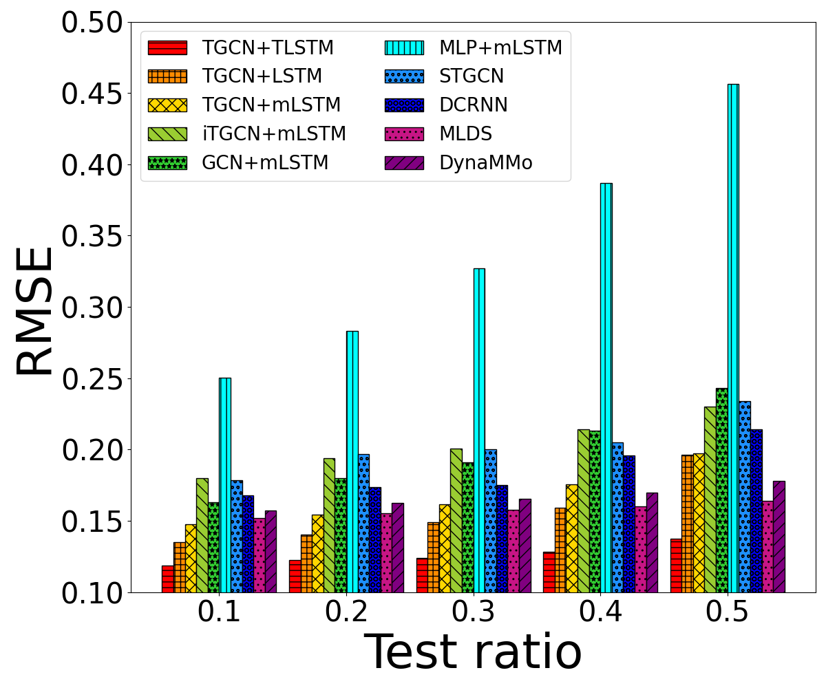
(a)

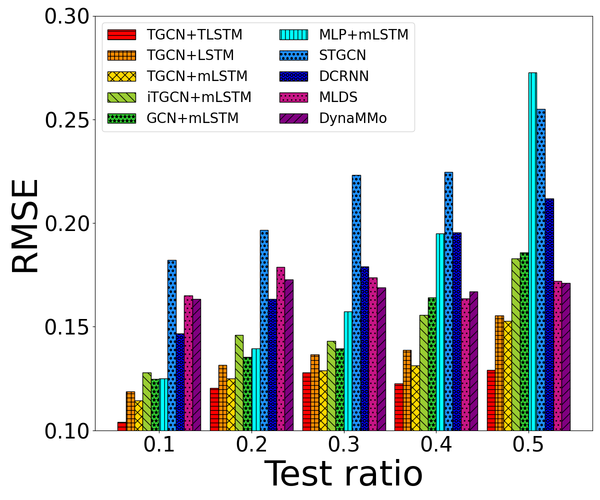
(b)

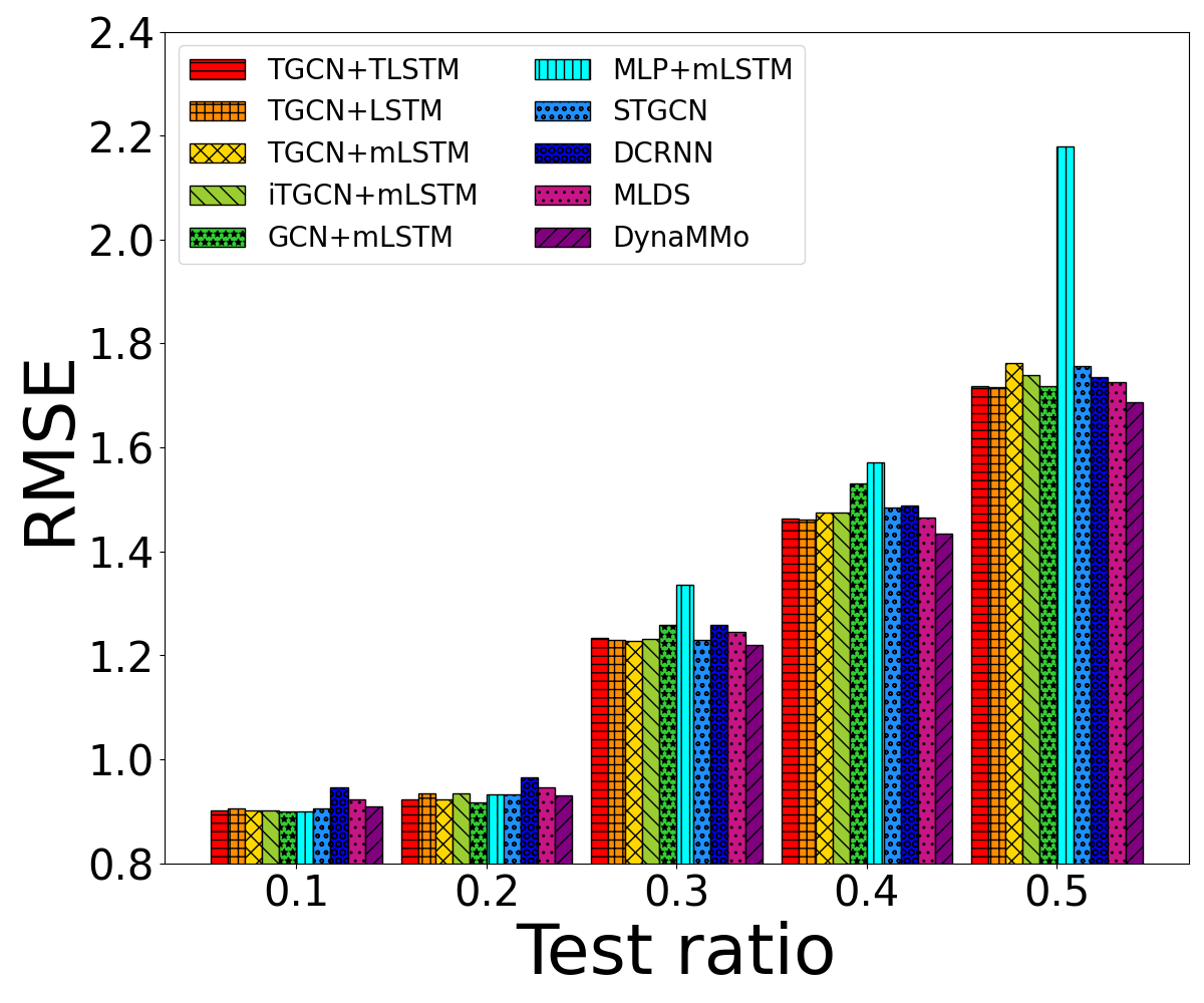
(c)

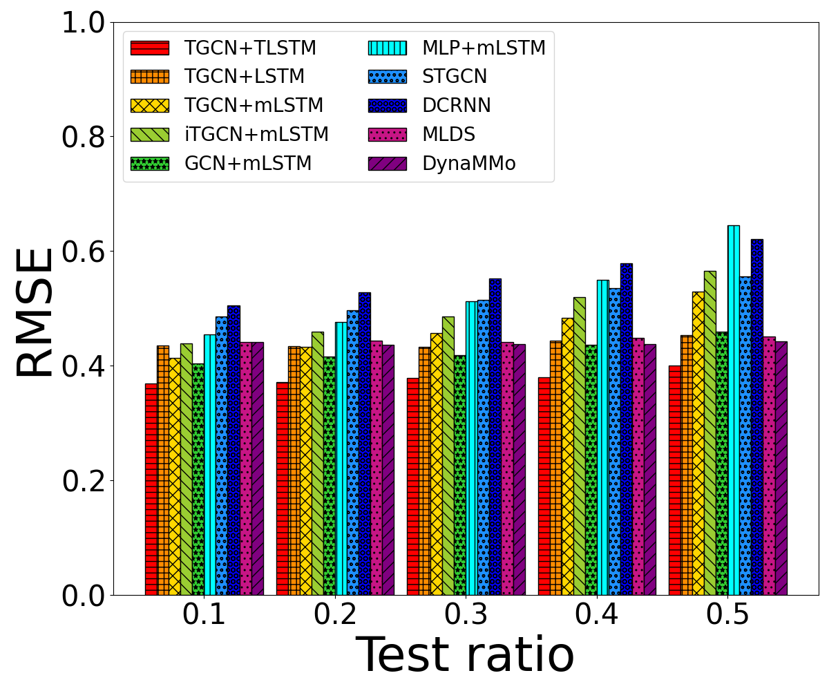
(d)

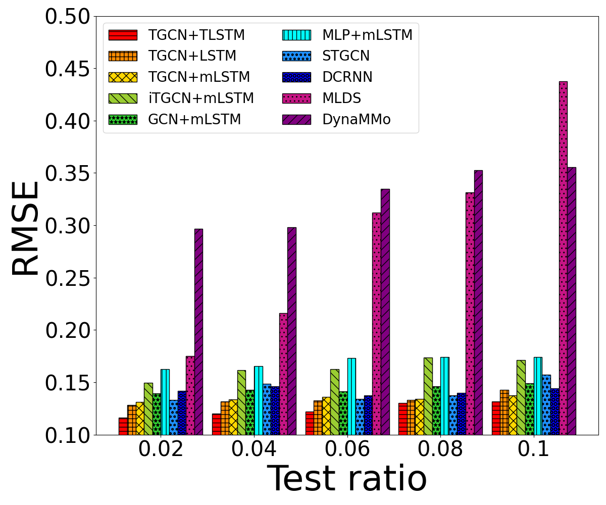
(e)

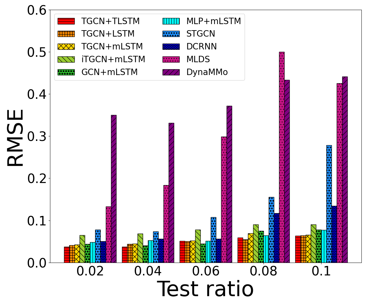
(f)

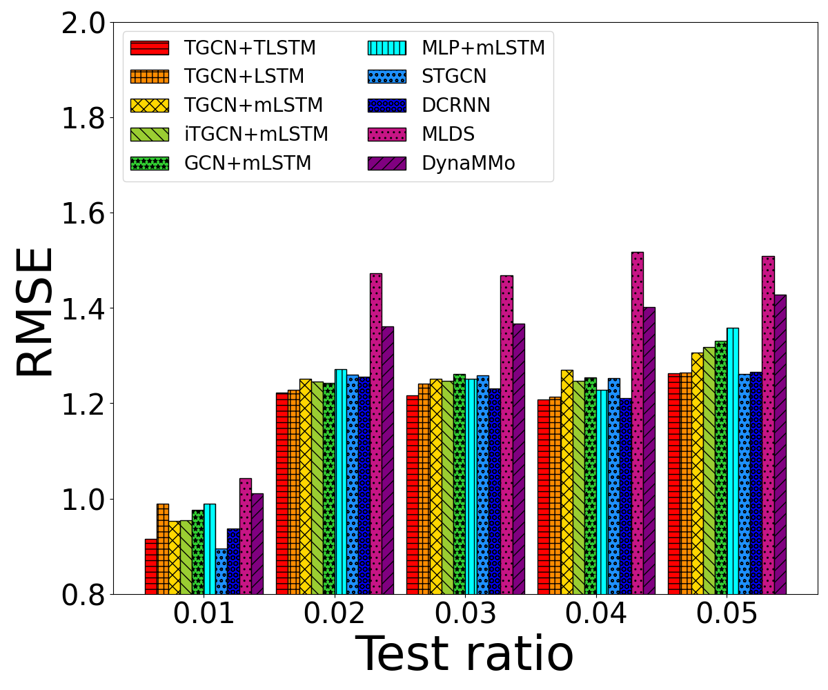
(g)

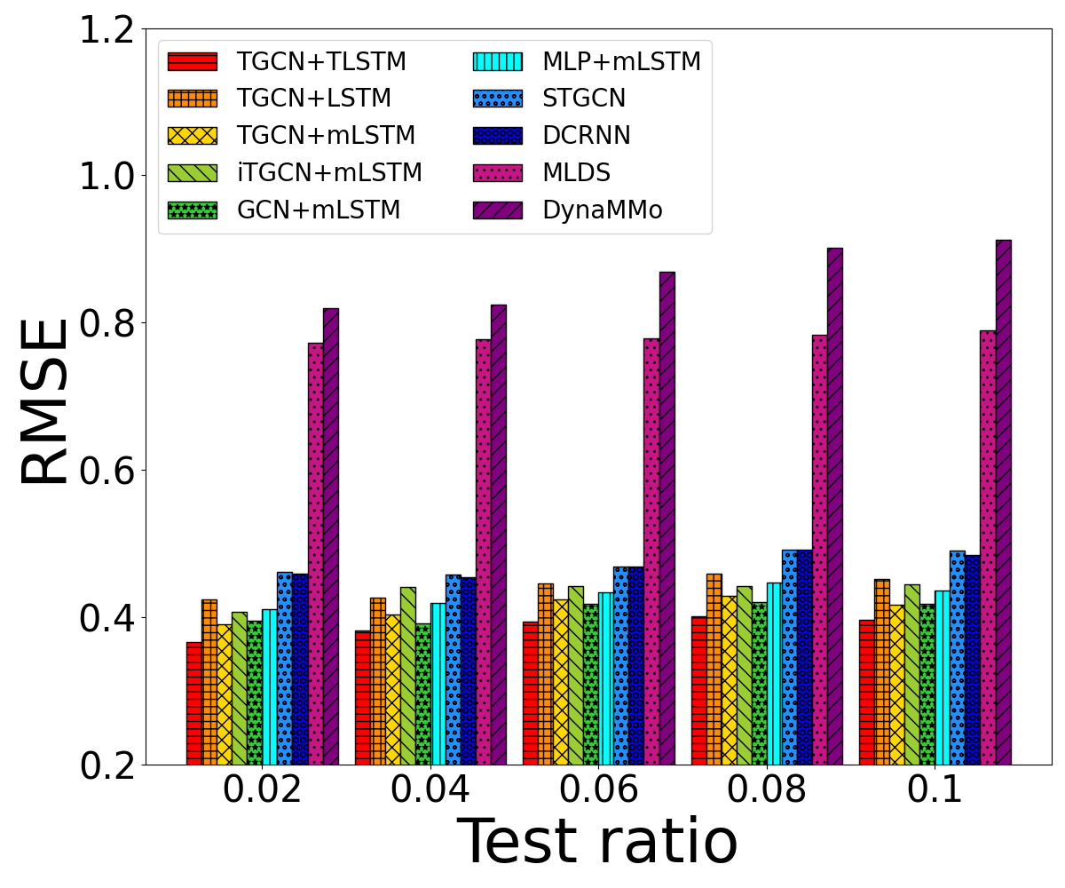
(h)

Figure 5. RMSE of missing value recovery (upper) and future value prediction (lower).

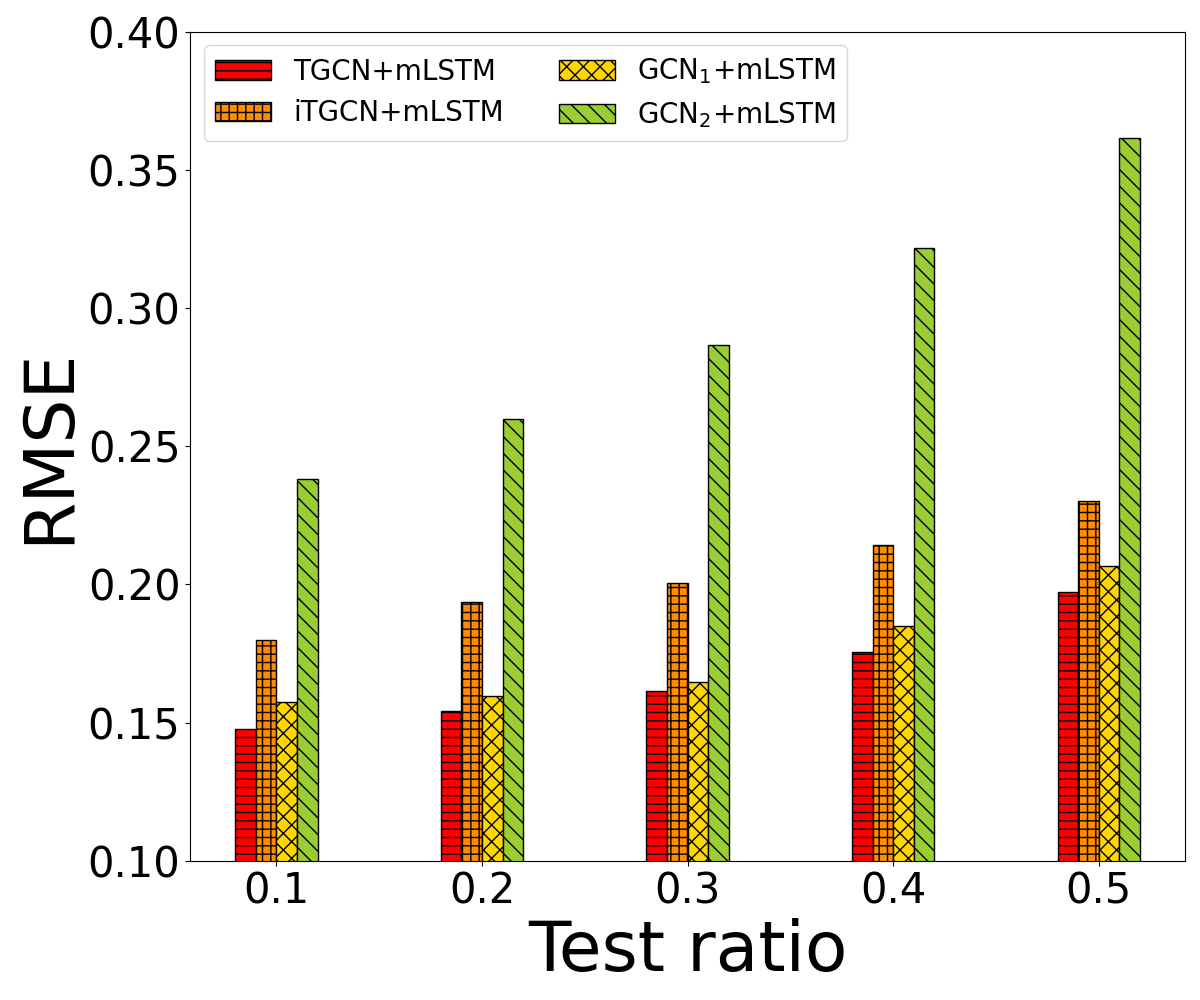
(a)

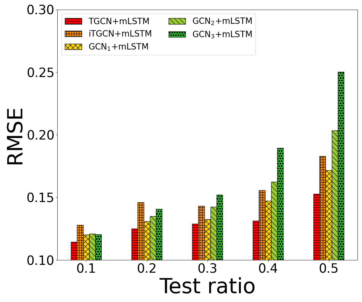
(b)

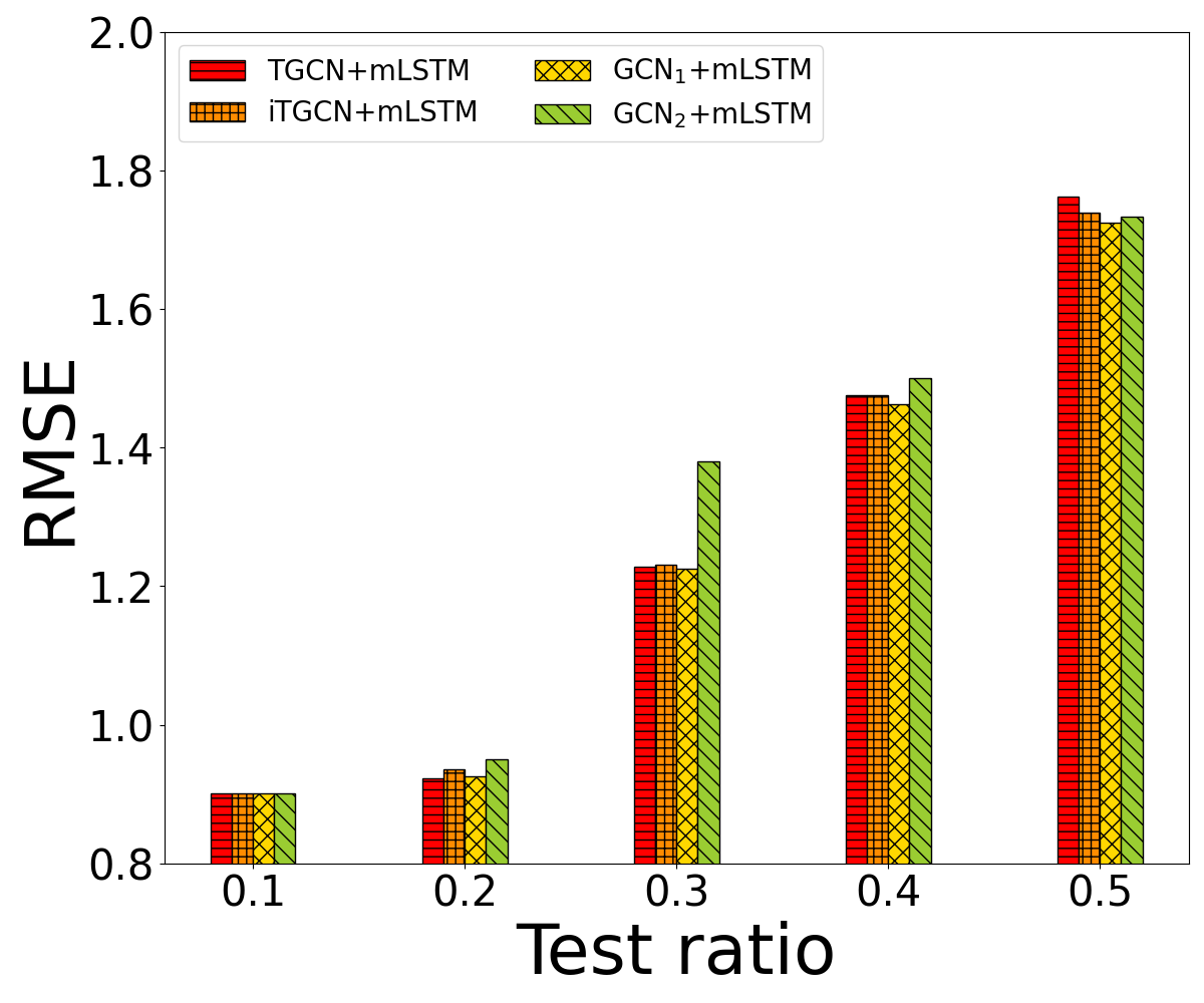
(c)

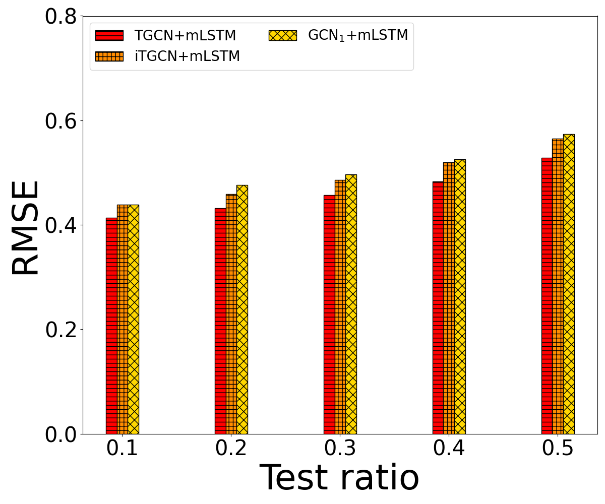
(d)

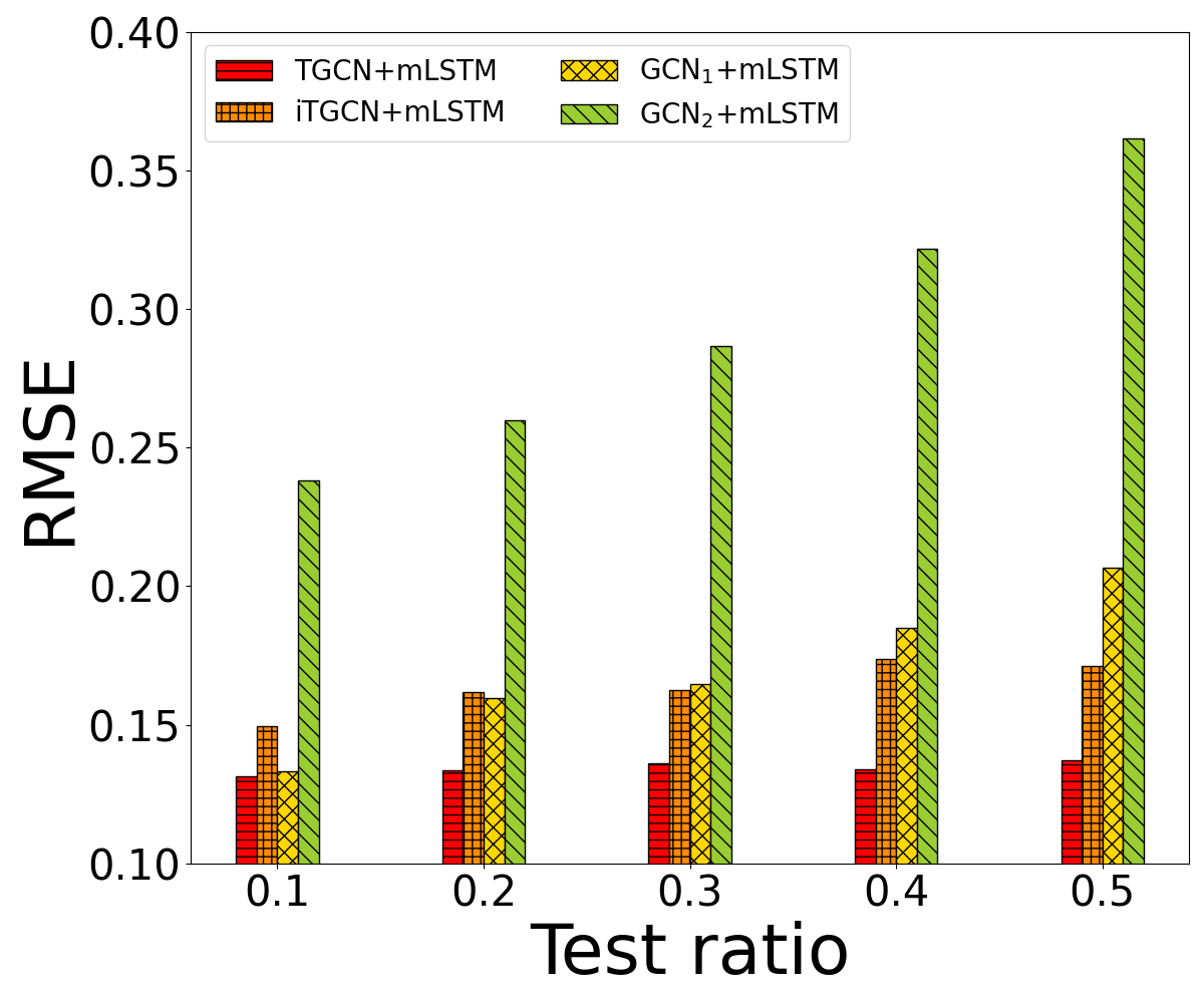
(e)

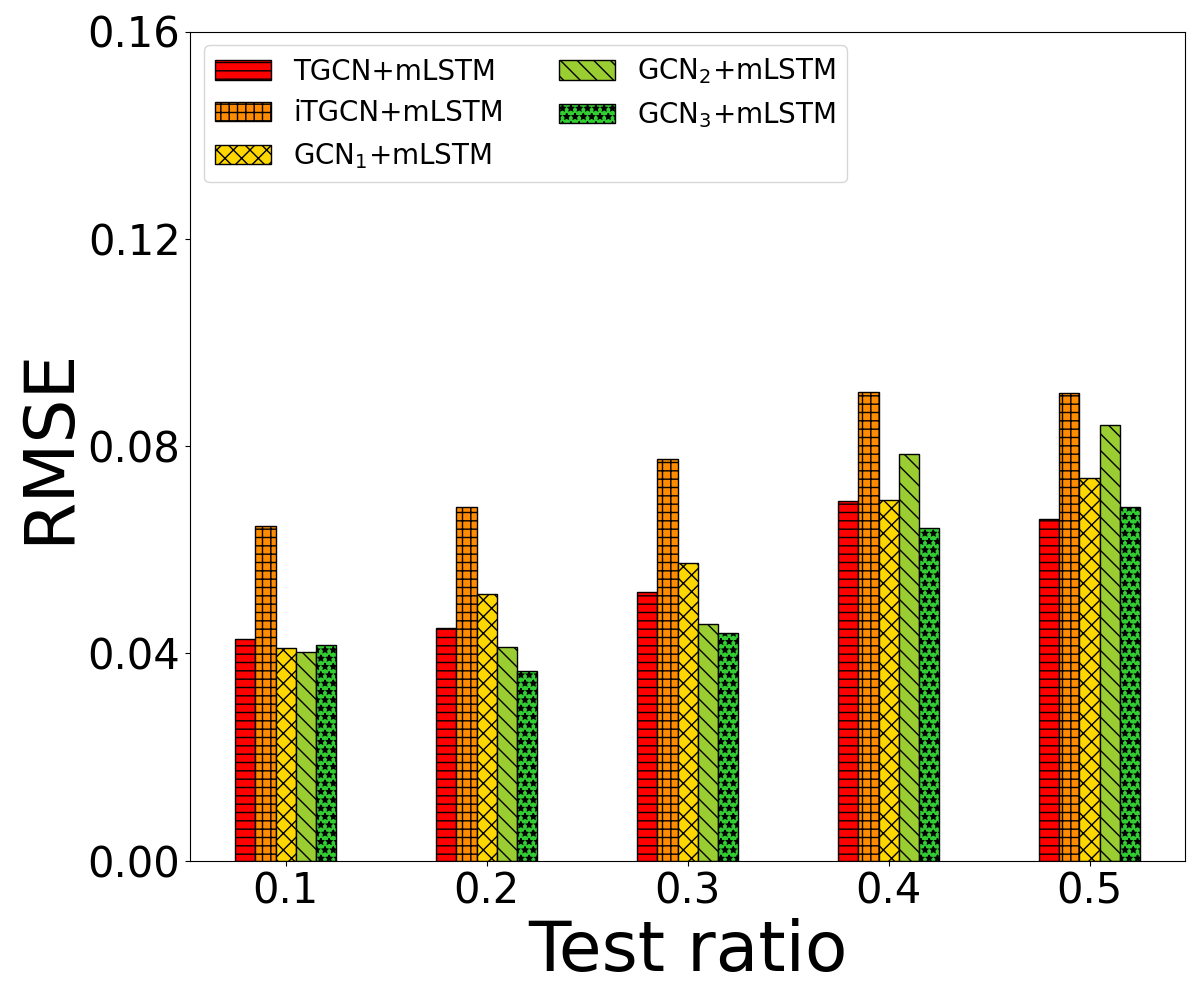
(f)

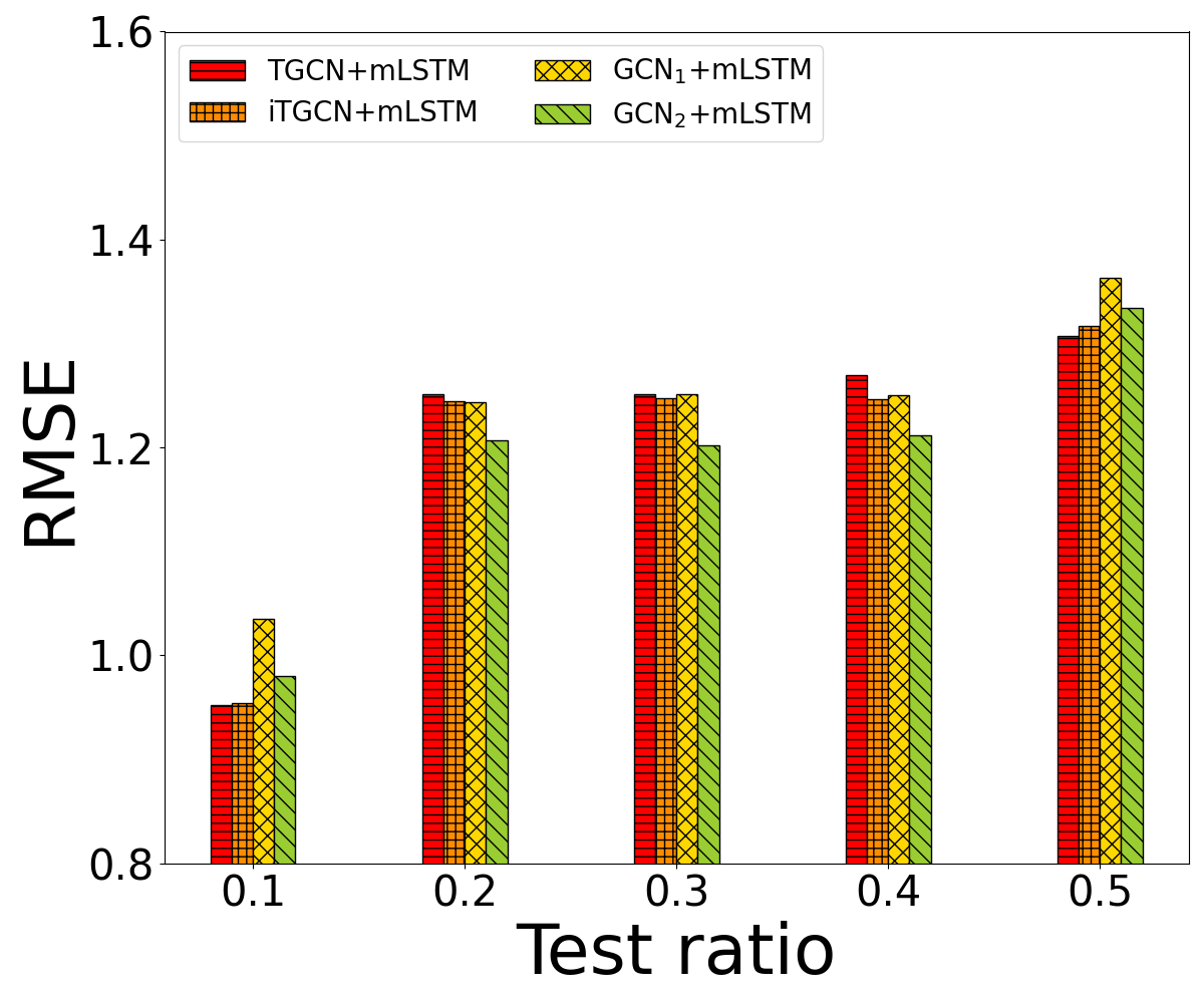
(g)

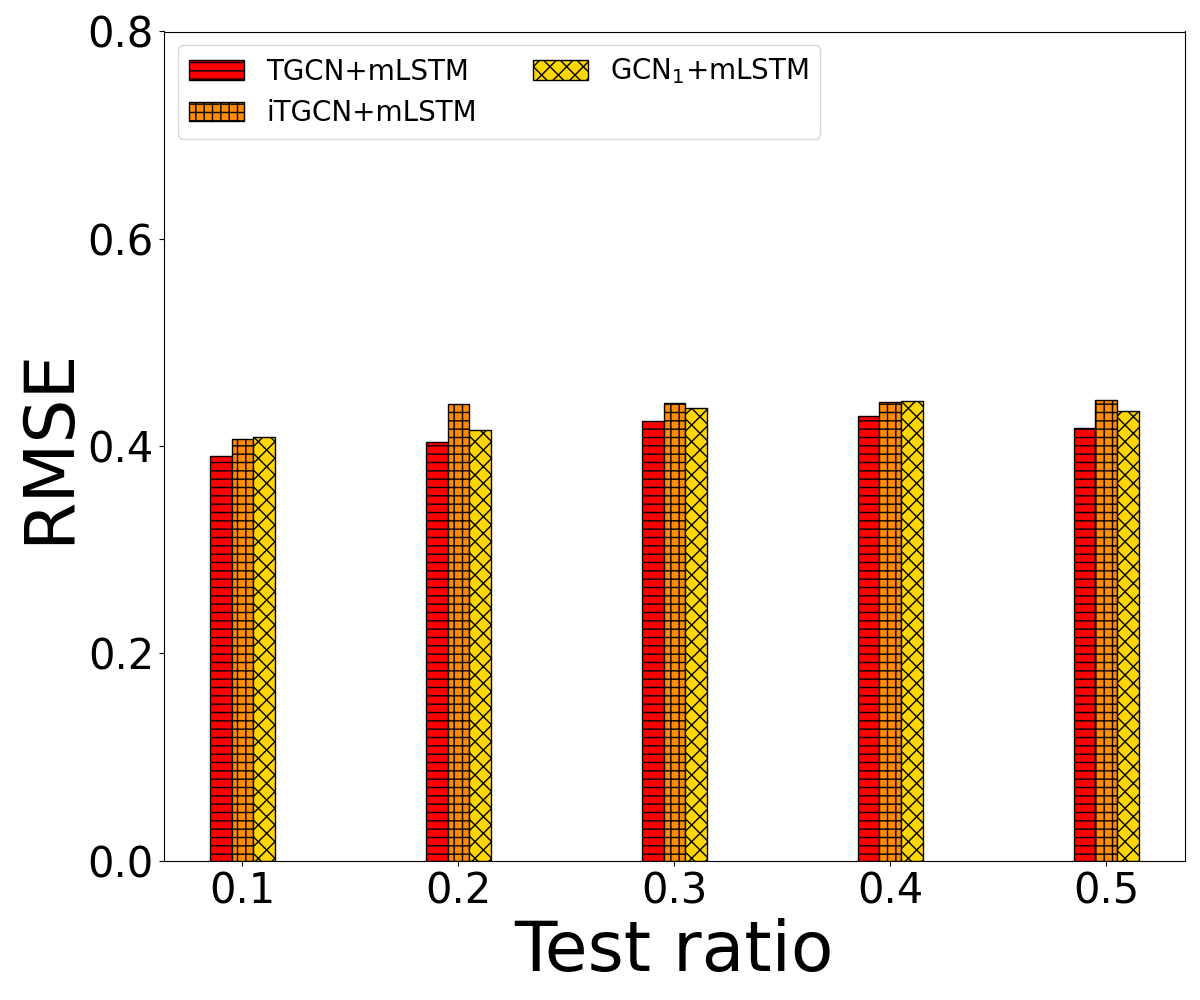
(h)

Figure 6. Synergy Analysis: RMSE of missing value recovery (upper) and future value prediction (lower).

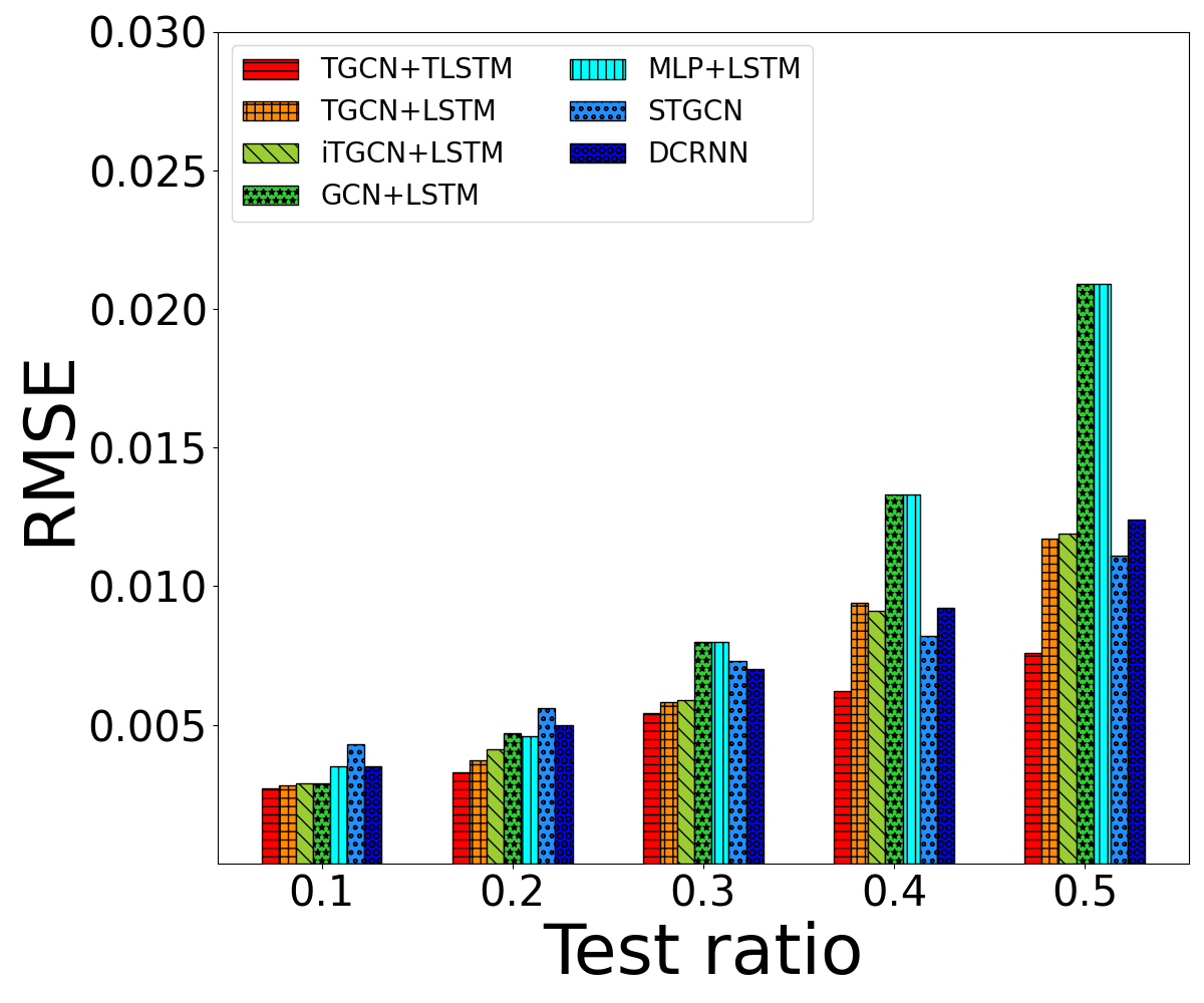
(a)

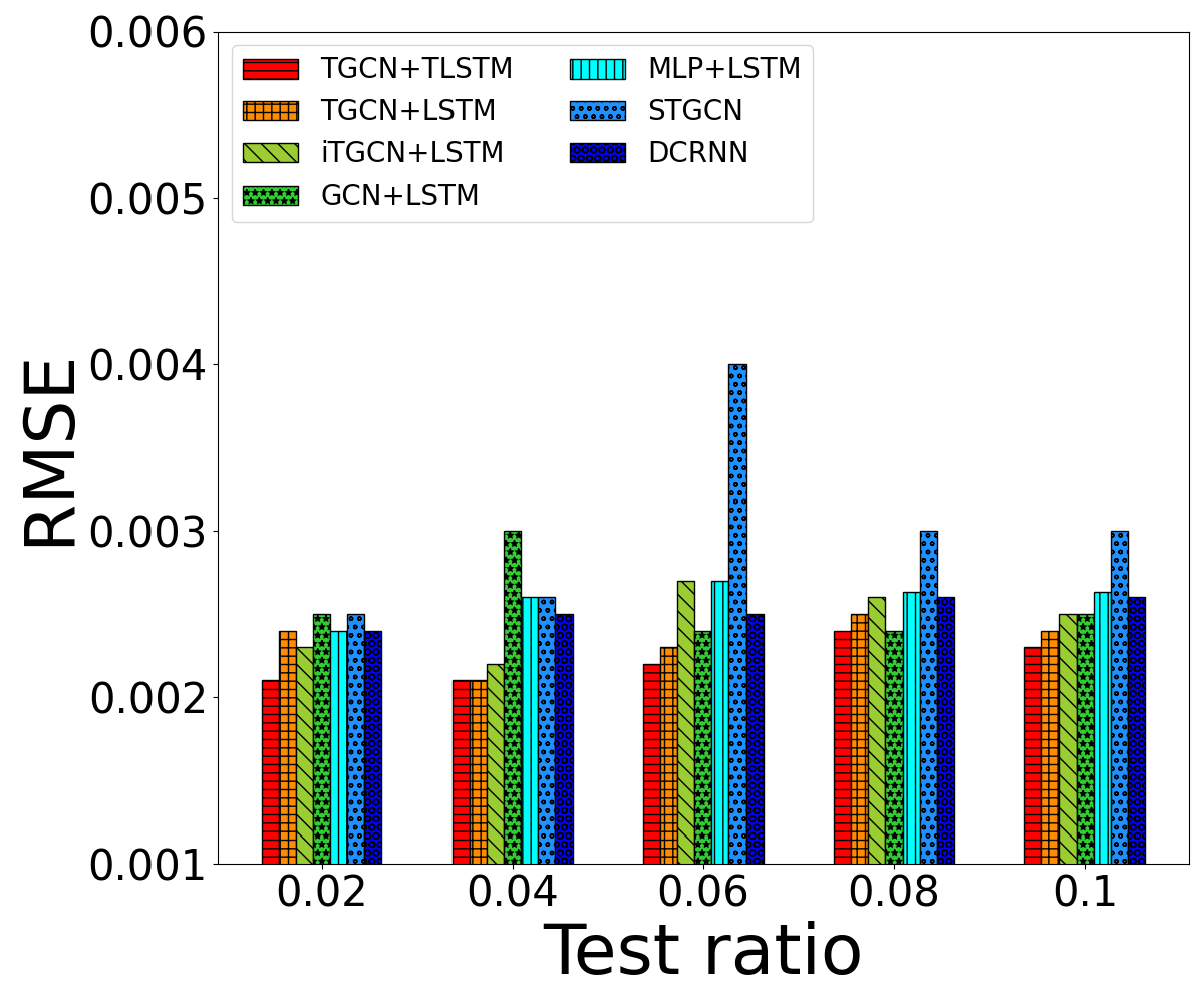
(b)

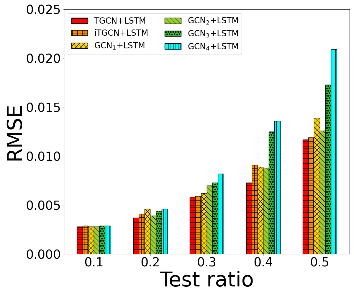
(c)

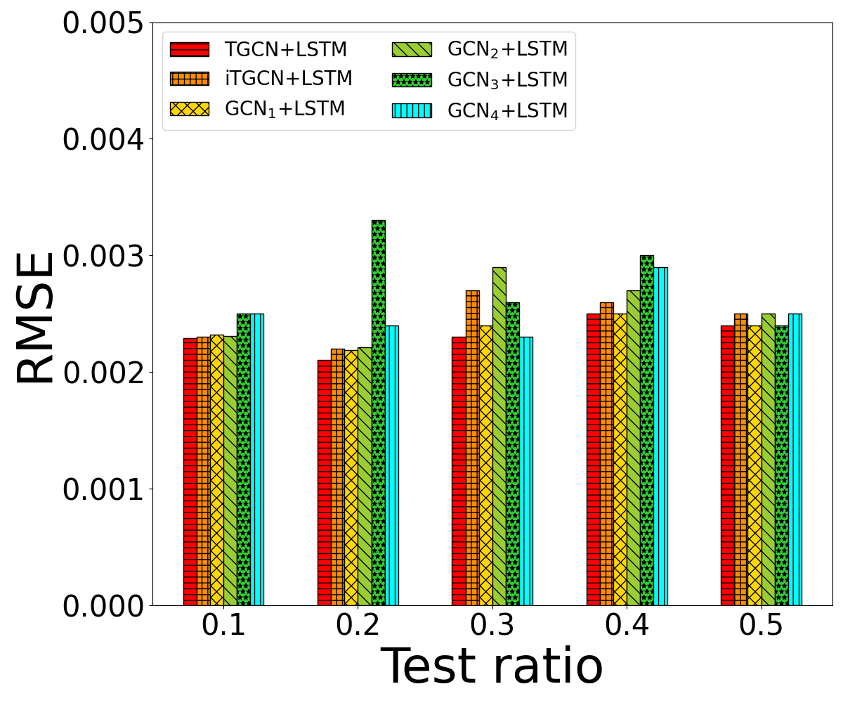
(d)

Figure 7. Experiments on the 20CR dataset

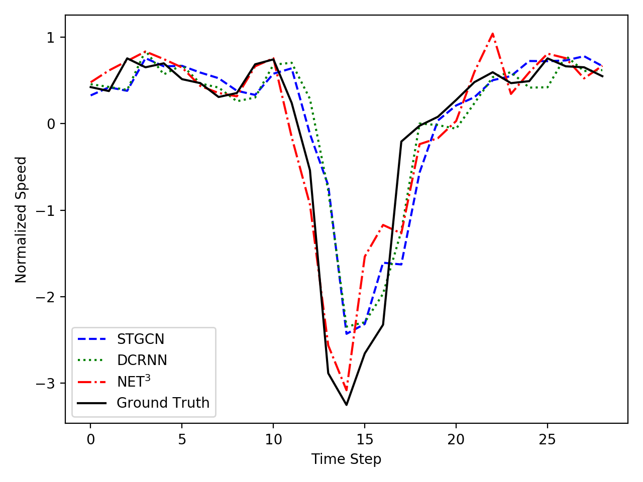
(a)

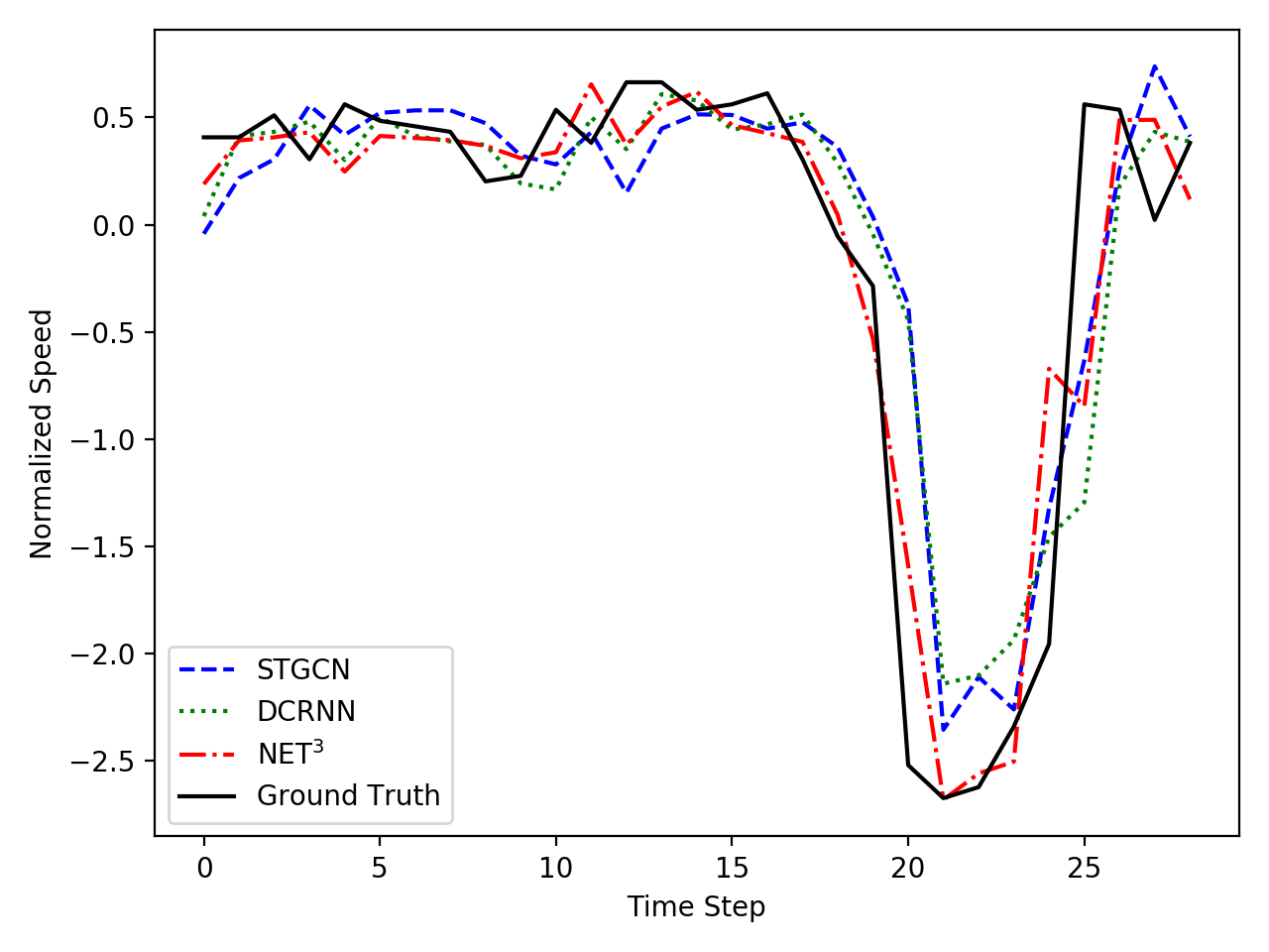
(b)

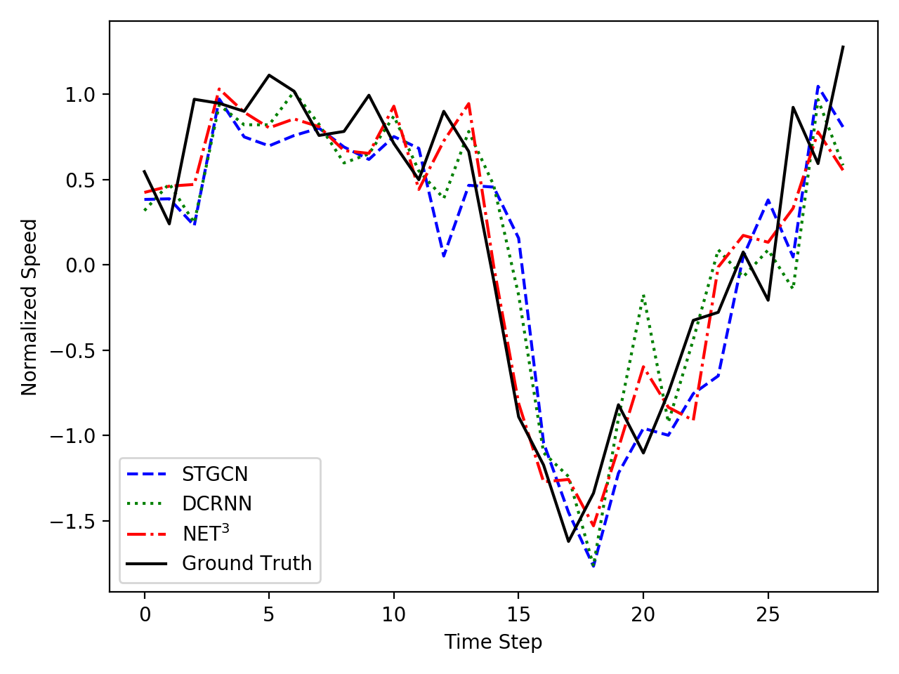
(c)

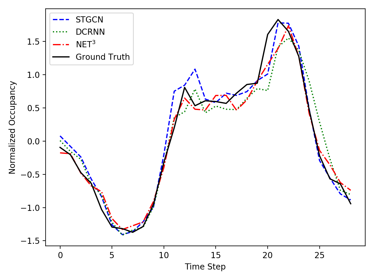
(d)

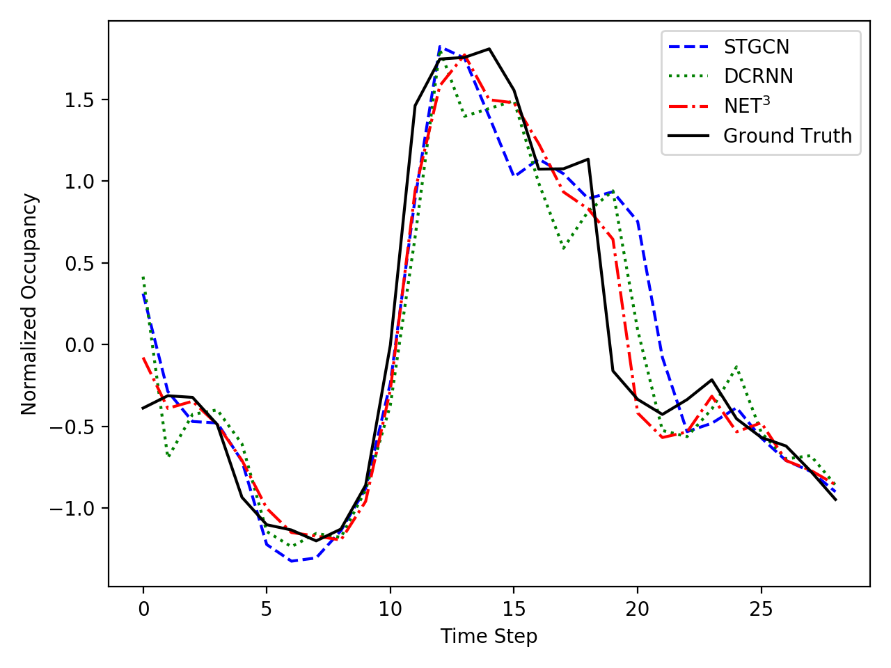
(e)

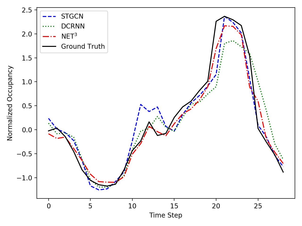
(f)

Figure 8. Visualization of future value prediction on the Traffic dataset. Upper part presents the results for normalized speed. Lower part presents the results for normalized occupancy.

4.1.3. Implementation Details

For all the datasets and tasks, we use one layer TGCN, one layer TLSTM, and one layer MLP with the linear activation. The hidden dimension is fixed as $8$. We fix $\rho=0.8$, $0.8$, $0.2$, $0.1$ and $0.9$ for TLSTM on Motes, Soil, Revenue, Traffic, and 20CR datasets respectively. The window size is set as $\omega=5$ and $\tau=1$, and Adam optimizer (Kingma and Ba, 2014) with a learning rate of $0.01$ is adopted. Coefficients $\mu_{1}$ and $\mu_{2}$ are fixed as $10^{-3}$.

4.2. Effectiveness Results

In this section, we present the effectiveness experimental results for missing value recovery, future value prediction, synergy analysis and sensitivity experiments.

4.2.1. Missing Value Recovery

For all the datasets, we randomly select 10% to 50% of the data points as test sets, and we use the mean and standard deviation of each time series in the training sets to normalize each time series. The evaluation results on Motes, Soil, Revenue and Traffic are shown in Figure 5(a)-5(d), and the results for 20CR are presented in 7(a). The proposed full model NeT³(TGCN+TLSTM) outperforms all of the baseline methods on almost all of the settings. Among the baselines methods, those equipped with GCNs generally have a better performance than LSTM. When comparing TGCN with iTGCN, we observe that TGCN performs better than iTGCN on most of the settings. This is due to TGCN’s capability in capturing various synergy among graphs. We can also observe that TLSTM (TGCN+TLSTM) achieves lower RMSE than both mLSTM (TGCN+mLSTM) and LSTM (TGCN+LSTM), demonstrating the effectiveness of capturing the implicit relations.

4.2.2. Future Value Prediction

We use the last 2% to 10% time steps as test sets for the Motes, Traffic, Soil and 20CR datasets, and we use the last 1% to 5% time steps as test sets for the Revenue dataset. Similar to the missing value recovery task, The datasets are normalized by mean and standard deviation of the training sets. The evaluation results are shown in Figure 5(e)-5(h) and Figure 7(b). The proposed NeT³ outperforms the baseline methods on all of the five datasets. Different from the missing value recovery task, the classic methods perform much worse than deep learning methods on the future value prediction, which might result from the fact that these methods are unable to capture the non-linearity in the temporal dynamics. Similar to the missing value recovery task, generally, TGCN also achives lower RMSE than iTGCN and GCN, and TLSTM performs better than both mLSTM and LSTM.

We present the visualization of the future value prediction task on the Traffic dataset in Figure 8.

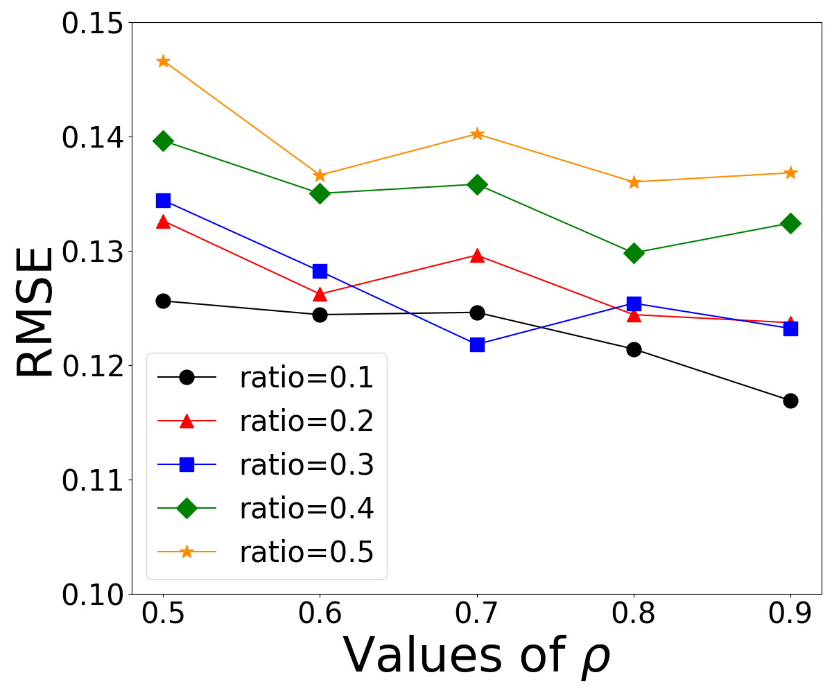
(a)

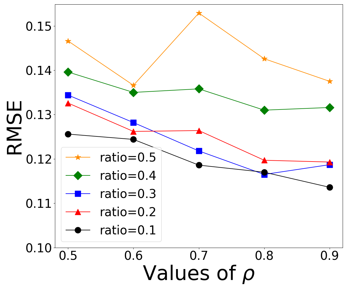
(b)

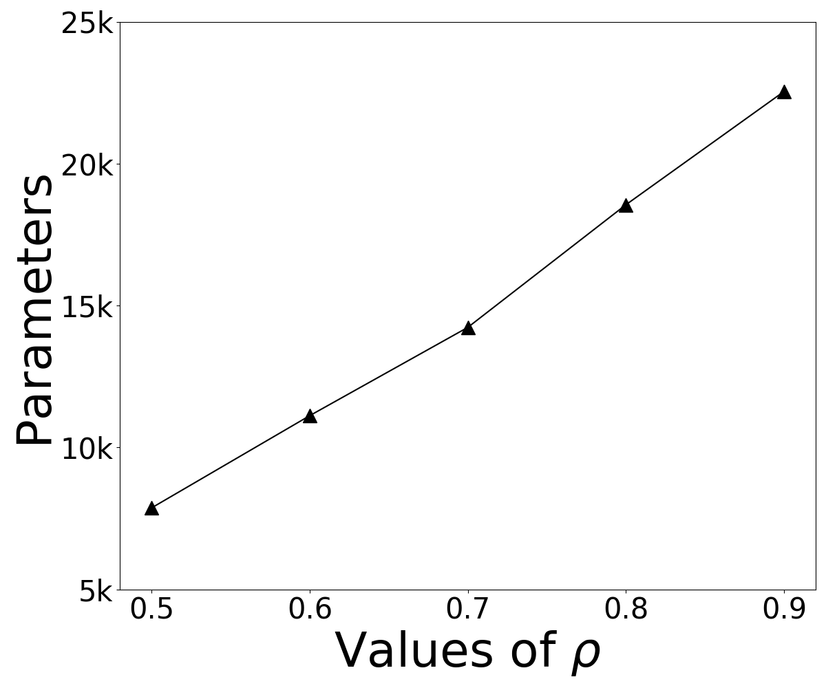
(c)

Figure 9. Sensitivity experiments of $\rho$ on the Motes dataset.

4.2.3. Experiments on Synergy

In this section, we compare the proposed TGCN with iTGCN, GCN₁, GCN₂, GCN₃ and GCN₄ (if applicable) on the missing value recovery and future value prediction tasks. Here, GCN₁, GCN₂, GCN₃ and GCN₄ denote the GCN with the adjacency matrix of the 1st, 2nd, 3rd and 4th mode respectively. iTGCN is an independent version of TGCN (Equation (41)), which is a simple linear combination of different GCNs (GCN₁, GCN₂, GCN₃ and GCN₄). As shown in Figure 6 and Figure 7(c)-7(d), generally, TGCN outperforms GCNs designed for single modes and the simple combination of them (iTGCN).

4.2.4. Sensitivity Experiments

We use different values of $\rho$ for TLSTM on the Motes dataset for the missing value recovery and future value prediction tasks and report their RMSE values in Figure 9(a) and Figure 9(b). It can be noted that, in general, the greater $\rho$ is, the better results (i.e., smaller RMSE) will be obtained. We believe the main reason is that a greater $\rho$ indicates that TLSTM captures more interaction between different time series. Figure 9(c) shows that the number of parameters of TLSTM is linear with respect to $\rho$.

Table 2. In the upper part, $\rho_{max}$ and $\rho_{exp}$ are the upper bounds and the values of $\rho$ used in experiments. The middle and lower parts present the number of parameters in TLSTM and LSTM, and the parameter reduction ratio.

	Motes	Soil	Revenue	Traffic	20CR
$\rho_{max}$	2.17	2.43	0.64	0.31	57.25
$\rho_{exp}$	0.80	0.80	0.20	0.10	0.90
TLSTM	18,552	10,996	87,967	180,554	16,696
mLSTM	117,504	57,120	669,120	1,088,000	58,752,000
Reduce	84.21%	80.75%	86.85%	83.40%	99.97%

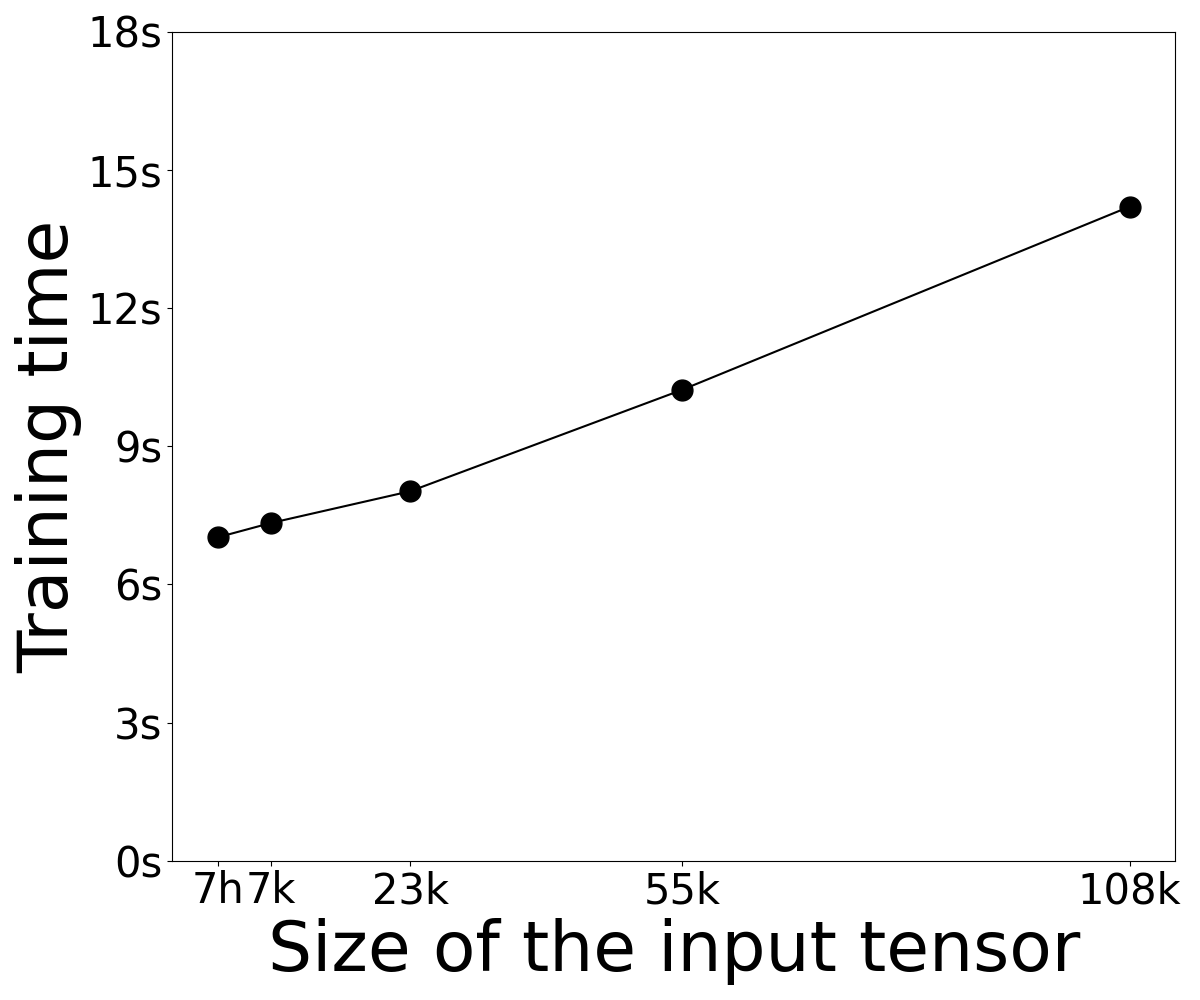
(a)

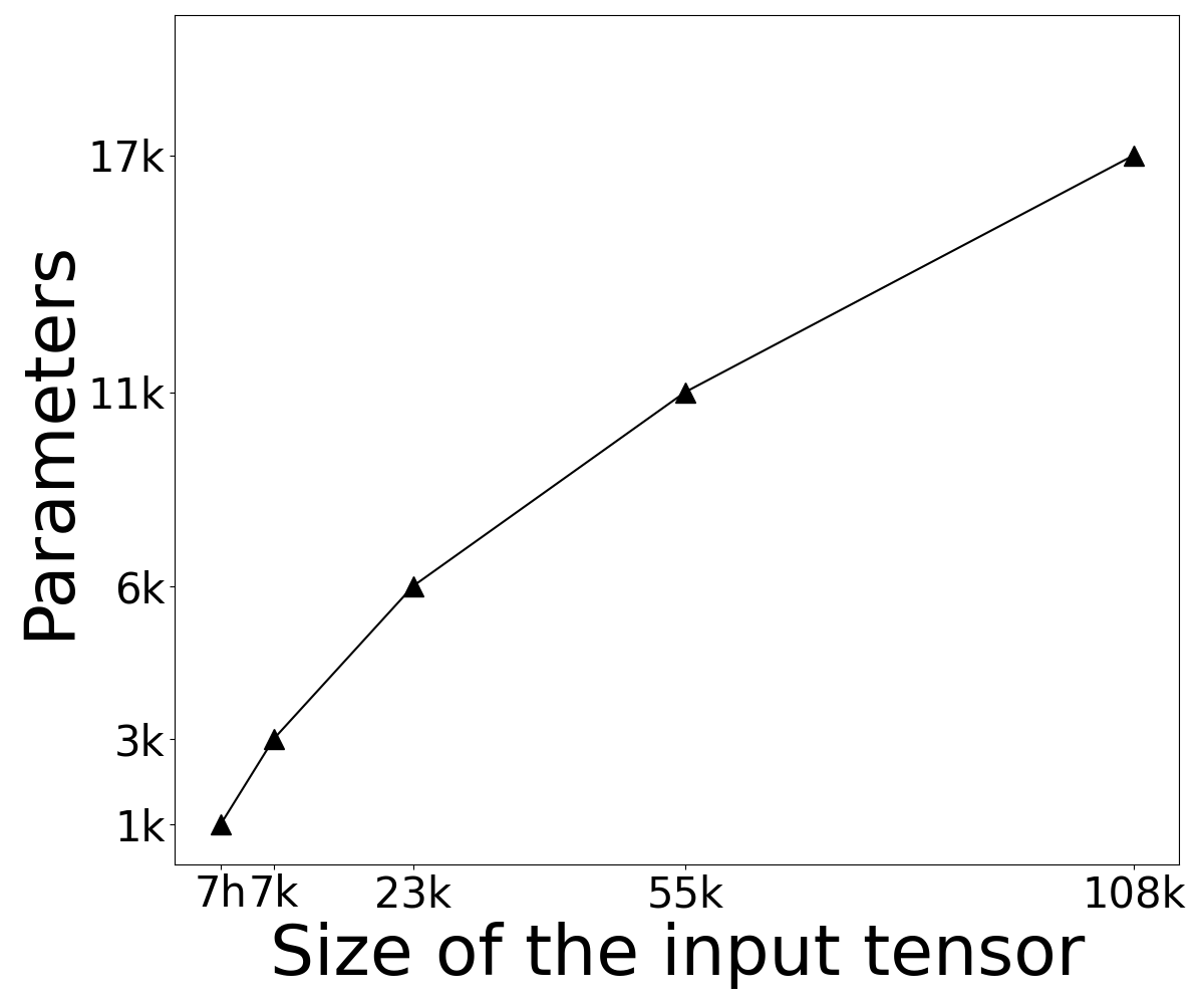
(b)

Figure 10. Scalability experiments.

4.3. Efficiency Results

In this section, we present experimental results for memory efficiency and scalability.

4.3.1. Memory Efficiency

As shown in Table 2, the upper bounds ($\rho_{max}$) of $\rho$ for the five datasets are 2.17, 2.43, 0.64, 0.31 and 57.25. In the experiments, we fix $\rho_{exp}=0.80$, $0.80$, $0.20$, $0.10$ and $0.90$ for the Motes, Soil, Revenue, Traffic and 20CR datasets, respectively. Given the above values of $\rho_{exp}$, the TLSTM row in Table 2 shows the number of parameters in TLSTM. The mLSTM row shows the required number of parameters for multiple separate LSTMs for each single time series. Compared with mLSTM, TLSTM significantly reduces the number of parameters by more than 80% and yet performs better than mLSTM (Figure 5 and Figure 7(a)-7(b)).

4.3.2. Scalability

We evaluate the scalability of NeT³on the 20CR dataset in terms of the training time and the number of parameters. We fix the $\rho=0.9$, and change the size of the input tensor by shrinking the dimension of all the modes by the specified ratios: [0.2, 0.4, 0.6, 0.8, 1.0]. Given the ratios, the input sizes (the number of nodes) are therefore 684, 6,912, 23,328, 55,296 and 108,000 respectively. The averaged training time of one epoch for TLSTM against the size of the input tensor is presented in left part of Figure 10, and the number of parameters of TLSTM against the size of the input tensor is presented in right part of Figure 10. Note that h and k on the x-axis represent hundreds and thousands respectively. s and k on the y-axis represent seconds and thousands respectively. The figures show that the training time and the number of parameters grow almost linearly with the size of input tensor.

5. Related Works

In this section, we review the related work in terms of (1) co-evolving time series, (2) graph convolutional networks (GCN), and (3) networked time series.

5.1. Co-evolving Time Series

Co-evolving time series is ubiquitous and appears in a variety of applications, such as enviornmental monitoring, financial analysis and smart transportation. Li et al. (Li et al., 2009) proposed a linear dynamic system based on Kalman filter and Bayesian networks to model co-evolving time series. Rogers et al. (Rogers et al., 2013) extended (Li et al., 2009) and further proposed a Multi-Linear Dynamic System (MLDS), which provides the base of the proposed TRNN. Yu et al (Yu et al., 2016) proposed a Temporal Regularized Matrix Factorization (TRMF) for modeling co-evolving time series. Zhou et al. (Zhou et al., 2016) proposed a bi-level model to detect the rare patterns of time series. Recently, Yu et al. (Yu et al., 2017a) used LSTM (Hochreiter and Schmidhuber, 1997) for modeling traffic flows. Liang et al. (Liang et al., 2018) proposed a multi-level attention network for geo-sensory time series prediction. Srivastava et al. (Srivastava and Lessmann, 2018) and Zhou et al. (Zhou and Huang, 2017) used separate RNNs for weather and air quality monitoring time series. Yu et al. (Yu et al., 2017c) proposed a HOT-RNN based on tensor-trains for long-term forecasting. Zhou et al. (Zhou et al., 2020) proposed a multi-domality neural attention network for financial time series. One limitation of this line of research is that it often ignores the relation network between different time series.

5.2. Graph Convolutional Networks

Plenty of real-world data could naturally be represented by a network or graph, such as social networks and sensor networks. Bruna et al. (Bruna et al., 2013) defined spectral graph convolution operation in the Fourier domain by analogizing it to one-dimensional convolution. Henaff et al. (Henaff et al., 2015) used a linear interpolation, and Defferrard et al. (Defferrard et al., 2016) adopted Chebyshev polynomials to approximate the spectral graph convolution. Kipf et al. (Kipf and Welling, 2016) simplified the Chebyshev approximation and proposed a GCN. These methods were typically designed for flat graphs. There are also graph convolutional network methods considering multiple types of relationships. Monti et al. (Monti et al., 2017) proposed a multi-graph CNN for matrix completion, which does not apply to tensor graphs. Wang et al. (Wang et al., 2019) proposed HAN which adopted attention mechanism to extract node embedding from different layers of a multiplex network (De Domenico et al., 2013; Jing et al., 2021; Yan et al., 2021), which is a flat graph with multiple types of relations, but not the tensor graph in our paper. Liu et al. (Liu et al., 2020) proposed a TensorGCN for text classification. It is worth pointing out that the term tensor in (Liu et al., 2020) was used in a different context, i.e., it actually refers to a multiplex graph. For a comprehensive review of the graph neural networks, please refer to (Zhang et al., 2019; Zhou et al., 2018; Wu et al., 2020).

5.3. Networked Time Series

Relation networks have been encoded into traditional machine learning methods such as dynamic linear (Li et al., 2009) and multi-linear (Rogers et al., 2013) systems for co-evolving time series (Cai et al., 2015a, b; Hairi et al., 2020). Recently, Li et al. (Li et al., 2017) incorporated spatial dependency of co-evolving traffic flows by the diffusion convolution. Yu et al. (Yu et al., 2017b) used GCN to incorporate spatial relations and CNN for capturing temporal dynamics. Yan et al. (Yan et al., 2018), introduced a spatial-temporal GCN for skeleton recognition. Li et al. (Li et al., 2019) leveraged RGCN (Schlichtkrull et al., 2018) to model spatial dependency and LSTM (Hochreiter and Schmidhuber, 1997) for temporal dynamics. These methods only focus on the relation graphs of a single mode, and ignore relations on other modes e.g. the correlation between the speed and occupancy of the traffic. In addition, these methods rely on the same function for capturing temporal dynamics of all time series.

It is worth pointing out that the proposed NeT³ unifies and supersedes both co-evolving time series and networked time series as a more general data model. For example, if the adjacency matrix $\mathbf{A}_{m}(m=1,...,M)$ for each mode is set as an identity matrix, the proposed NeT³ degenerates to co-evolving (tensor) time series (e.g., (Li et al., 2009)); networked time series in (Cai et al., 2015a) can be viewed as a special case of NeT³ whose tensor $\mathcal{X}$ only has a single mode.

6. Conclusion

In this paper, we introduce a novel NeT³ for jointly modeling of tensor time series with its relation networks. In order to effectively model the tensor with its relation networks at each time step, we generalize the graph convolution from flat graphs to tensor graphs and propose a novel TGCN which not only captures the synergy among graphs but also has a succinct form. To balance the commonality and specificity of the co-evolving time series, we propose a novel TRNN, which helps reduce noise in the data and the number of parameters in the model. Experiments on a variety of real-world datasets demonstrate the efficacy and the applicability of NeT³.

- (1)
- Akoglu et al. (2015) Leman Akoglu, Hanghang Tong, and Danai Koutra. 2015. Graph based anomaly detection and description: a survey. Data mining and knowledge discovery 29, 3 (2015), 626–688.
- Banzon et al. (2016) Viva Banzon, Thomas M Smith, Toshio Mike Chin, Chunying Liu, and William Hankins. 2016. A long-term record of blended satellite and in situ sea-surface temperature for climate monitoring, modeling and environmental studies. Earth System Science Data 8, 1 (2016), 165–176.
- Barnett (1941) Martin K Barnett. 1941. A brief history of thermometry. Journal of Chemical Education 18, 8 (1941), 358.
- Bodik et al. (2004) Peter Bodik, Wei Hong, Carlos Guestrin, Sam Madden, Mark Paskin, and Romain Thibau. 2004. Motes Dataset. http://db.csail.mit.edu/labdata/labdata.html
- Bruna et al. (2013) Joan Bruna, Wojciech Zaremba, Arthur Szlam, and Yann LeCun. 2013. Spectral networks and locally connected networks on graphs. arXiv preprint arXiv:1312.6203 (2013).
- Cai et al. (2015a) Yongjie Cai, Hanghang Tong, Wei Fan, and Ping Ji. 2015a. Fast mining of a network of coevolving time series. In Proceedings of the 2015 SIAM International Conference on Data Mining. SIAM, 298–306.
- Cai et al. (2015b) Yongjie Cai, Hanghang Tong, Wei Fan, Ping Ji, and Qing He. 2015b. Facets: Fast comprehensive mining of coevolving high-order time series. In KDD.
- Chakrabarti and Faloutsos (2006) Deepayan Chakrabarti and Christos Faloutsos. 2006. Graph mining: Laws, generators, and algorithms. ACM computing surveys (CSUR) 38, 1 (2006), 2–es.
- Compo et al. (2011) Gilbert P Compo, Jeffrey S Whitaker, Prashant D Sardeshmukh, Nobuki Matsui, Robert J Allan, Xungang Yin, Byron E Gleason, Russell S Vose, Glenn Rutledge, Pierre Bessemoulin, et al. 2011. The twentieth century reanalysis project. Quarterly Journal of the Royal Meteorological Society 137, 654 (2011), 1–28.
- De Domenico et al. (2013) Manlio De Domenico, Albert Solé-Ribalta, Emanuele Cozzo, Mikko Kivelä, Yamir Moreno, Mason A Porter, Sergio Gómez, and Alex Arenas. 2013. Mathematical formulation of multilayer networks. Physical Review X 3, 4 (2013), 041022.
- Defferrard et al. (2016) Michaël Defferrard, Xavier Bresson, and Pierre Vandergheynst. 2016. Convolutional neural networks on graphs with fast localized spectral filtering. arXiv preprint arXiv:1606.09375 (2016).
- Gasch et al. (2017) Caley K Gasch, David J Brown, Erin S Brooks, Matt Yourek, Matteo Poggio, Douglas R Cobos, and Colin S Campbell. 2017. A pragmatic, automated approach for retroactive calibration of soil moisture sensors using a two-step, soil-specific correction. Computers and Electronics in Agriculture 137 (2017), 29–40.
- Hairi et al. (2020) N Hairi, Hanghang Tong, and Lei Ying. 2020. NetDyna: Mining Networked Coevolving Time Series with Missing Values. In IEEE International Conference on Big Data.
- Henaff et al. (2015) Mikael Henaff, Joan Bruna, and Yann LeCun. 2015. Deep convolutional networks on graph-structured data. arXiv preprint arXiv:1506.05163 (2015).
- Hochreiter and Schmidhuber (1997) Sepp Hochreiter and Jürgen Schmidhuber. 1997. Long short-term memory. Neural computation 9, 8 (1997), 1735–1780.
- Jing et al. (2021) Baoyu Jing, Chanyoung Park, and Hanghang Tong. 2021. HDMI: High-order Deep Multiplex Infomax. arXiv preprint arXiv:2102.07810 (2021).
- Kingma and Ba (2014) Diederik P Kingma and Jimmy Ba. 2014. Adam: A method for stochastic optimization. arXiv preprint arXiv:1412.6980 (2014).
- Kipf and Welling (2016) Thomas N Kipf and Max Welling. 2016. Semi-supervised classification with graph convolutional networks. arXiv preprint arXiv:1609.02907 (2016).
- Kolda and Bader (2009) Tamara G Kolda and Brett W Bader. 2009. Tensor decompositions and applications. SIAM review 51, 3 (2009), 455–500.
- Lee et al. (2015) Charles MC Lee, Paul Ma, and Charles CY Wang. 2015. Search-based peer firms: Aggregating investor perceptions through internet co-searches. Journal of Financial Economics 116, 2 (2015), 410–431.
- Li et al. (2019) Jia Li, Zhichao Han, Hong Cheng, Jiao Su, Pengyun Wang, Jianfeng Zhang, and Lujia Pan. 2019. Predicting path failure in time-evolving graphs. In Proceedings of the 25th ACM SIGKDD International Conference on Knowledge Discovery & Data Mining. 1279–1289.
- Li et al. (2009) Lei Li, James McCann, Nancy S Pollard, and Christos Faloutsos. 2009. Dynammo: Mining and summarization of coevolving sequences with missing values. In Proceedings of the 15th ACM SIGKDD international conference on Knowledge discovery and data mining. 507–516.
- Li et al. (2017) Yaguang Li, Rose Yu, Cyrus Shahabi, and Yan Liu. 2017. Diffusion convolutional recurrent neural network: Data-driven traffic forecasting. arXiv preprint arXiv:1707.01926 (2017).
- Liang et al. (2018) Yuxuan Liang, Songyu Ke, Junbo Zhang, Xiuwen Yi, and Yu Zheng. 2018. Geoman: Multi-level attention networks for geo-sensory time series prediction.. In IJCAI. 3428–3434.
- Liu et al. (2020) Xien Liu, Xinxin You, Xiao Zhang, Ji Wu, and Ping Lv. 2020. Tensor graph convolutional networks for text classification. In Proceedings of the AAAI Conference on Artificial Intelligence, Vol. 34. 8409–8416.
- Monti et al. (2017) Federico Monti, Michael M Bronstein, and Xavier Bresson. 2017. Geometric matrix completion with recurrent multi-graph neural networks. arXiv preprint arXiv:1704.06803 (2017).
- Rogers et al. (2013) Mark Rogers, Lei Li, and Stuart J Russell. 2013. Multilinear dynamical systems for tensor time series. Advances in Neural Information Processing Systems 26 (2013), 2634–2642.
- Schlichtkrull et al. (2018) Michael Schlichtkrull, Thomas N Kipf, Peter Bloem, Rianne Van Den Berg, Ivan Titov, and Max Welling. 2018. Modeling relational data with graph convolutional networks. In European semantic web conference. Springer, 593–607.
- Slivinski et al. (2019) Laura C Slivinski, Gilbert P Compo, Jeffrey S Whitaker, Prashant D Sardeshmukh, Benjamin S Giese, Chesley McColl, Rob Allan, Xungang Yin, Russell Vose, Holly Titchner, et al. 2019. Towards a more reliable historical reanalysis: Improvements for version 3 of the Twentieth Century Reanalysis system. Quarterly Journal of the Royal Meteorological Society 145, 724 (2019), 2876–2908.
- Srivastava and Lessmann (2018) Shikhar Srivastava and Stefan Lessmann. 2018. A comparative study of LSTM neural networks in forecasting day-ahead global horizontal irradiance with satellite data. Solar Energy 162 (2018), 232–247.
- Sutskever (2013) Ilya Sutskever. 2013. Training recurrent neural networks. University of Toronto Toronto, Canada.
- Tsay (2014) Ruey S Tsay. 2014. Financial time series. Wiley StatsRef: Statistics Reference Online (2014), 1–23.
- Wang et al. (2019) Xiao Wang, Houye Ji, Chuan Shi, Bai Wang, Yanfang Ye, Peng Cui, and Philip S Yu. 2019. Heterogeneous graph attention network. In The World Wide Web Conference. 2022–2032.
- Wu et al. (2020) Zonghan Wu, Shirui Pan, Fengwen Chen, Guodong Long, Chengqi Zhang, and S Yu Philip. 2020. A comprehensive survey on graph neural networks. IEEE transactions on neural networks and learning systems (2020).
- Yan et al. (2018) Sijie Yan, Yuanjun Xiong, and Dahua Lin. 2018. Spatial temporal graph convolutional networks for skeleton-based action recognition. In Proceedings of the AAAI conference on artificial intelligence, Vol. 32.
- Yan et al. (2021) Yuchen Yan, Lihui Liu, Yikun Ban, Baoyu Jing, and Hanghang Tong. 2021. Dynamic Knowledge Alignment. In AAAI.
- Yu et al. (2017b) Bing Yu, Haoteng Yin, and Zhanxing Zhu. 2017b. Spatio-temporal graph convolutional networks: A deep learning framework for traffic forecasting. arXiv preprint arXiv:1709.04875 (2017).
- Yu et al. (2016) Hsiang-Fu Yu, Nikhil Rao, and Inderjit S Dhillon. 2016. Temporal Regularized Matrix Factorization for High-dimensional Time Series Prediction.. In NIPS. 847–855.
- Yu et al. (2017a) Rose Yu, Yaguang Li, Cyrus Shahabi, Ugur Demiryurek, and Yan Liu. 2017a. Deep learning: A generic approach for extreme condition traffic forecasting. In Proceedings of the 2017 SIAM international Conference on Data Mining. SIAM, 777–785.
- Yu et al. (2017c) Rose Yu, Stephan Zheng, Anima Anandkumar, and Yisong Yue. 2017c. Long-term forecasting using tensor-train rnns. Arxiv (2017).
- Zhang et al. (2019) Si Zhang, Hanghang Tong, Jiejun Xu, and Ross Maciejewski. 2019. Graph convolutional networks: a comprehensive review. Computational Social Networks (2019).
- Zhou et al. (2016) D. Zhou, J. He, Y. Cao, and J. Seo. 2016. Bi-Level Rare Temporal Pattern Detection. In 2016 IEEE 16th International Conference on Data Mining (ICDM). 719–728. https://doi.org/10.1109/ICDM.2016.0083
- Zhou et al. (2020) Dawei Zhou, Lecheng Zheng, Yada Zhu, Jianbo Li, and Jingrui He. 2020. Domain adaptive multi-modality neural attention network for financial forecasting. In Proceedings of The Web Conference 2020. 2230–2240.
- Zhou et al. (2018) Jie Zhou, Ganqu Cui, Zhengyan Zhang, Cheng Yang, Zhiyuan Liu, Lifeng Wang, Changcheng Li, and Maosong Sun. 2018. Graph neural networks: A review of methods and applications. arXiv preprint arXiv:1812.08434 (2018).
- Zhou and Huang (2017) Jingguang Zhou and Zili Huang. 2017. Recover missing sensor data with iterative imputing network. arXiv preprint arXiv:1711.07878 (2017).