Multifractal wave functions of charge carriers in graphene with folded deformations, ripples or uniaxial flexural modes: analogies to the quantum Hall effect under random pseudomagnetic fields.

Abstract

The electronic behavior in graphene under arbitrary uniaxial deformations, such as foldings or flexural fields is studied by including in the Dirac equation pseudoelectromagnetic fields. General foldings are thus studied by showing that uniaxial deformations can be considered pseudomagnetic fields in the Coulomb gauge norm. This allows to give an expression for the Fermi (zero) energy modes wavefunctions. For random deformations, contact is made with previous works on the quantum Hall effect under random magnetic fields, showing that the density of states has a power law behavior and that the zero energy modes wavefunctions are multifractal. This hints at an unusual electron velocity distribution. Also, it is shown that a strong Aharonov-Bohm pseudo-effect is produced. For more general non-uniaxial general flexural strain, it is not possible to use the Coulomb gauge. The results presented here helps to tailor-made graphene uniaxial deformations to achieve specific wave-functions.

I Introduction

Recently, Dirac materials have attracted intense research interest following the celebrated discovery of a two-dimensional (2D) hexagonal allotropic atomic carbon, graphene Novoselov666 , because of its peculiar band structure and its fascinating properties AlessandroCresti2008 ; LuisEF2014 largely due to the massless Dirac fermion behavior of the charge carriers.

Due to such excellent mechanical, magnetic and thermal properties of graphite monolayers, they can be used for the development of superconducting devices for micro-electromechanical and nano-electromechanical systems, leading to the development of the next generation of nanoelectronics RevModPhys.81.109 ; RevModPhys.83.407 . As the use of graphene sheets increases, the understanding of the mechanical behaviour is necessary and important for the design and analysis of graphene nanostructures and nanosystems. This opened a new field of research known as straintronics, which aims to refine the electronic and optical properties by applying mechanical deformations Naumis2017 . Following this direction, many theoretical works have been made studying the effect of mechanical strains on the electronic properties GGNaumis2009 ; Rodriguez2016 using a tight-binding approach Zhang2010 ; Zhang2011 and effective Hamiltonians for low energies in the vicinity of Dirac points Vozmediano2010 ; Oliva2013 ; Oliva2015 ; Guinea2009 . These electronic degrees of freedom are coupled to the structural lattice deformations, and this allows to modify its electronic properties in interesting ways Vozmediano2010 ; Amorim2015 ; Bastos2014 ; Chen2016 ; Deji2017 . It has been shown that a model to describe the coupling of the electrons to the out-of-plane deformation should be the Dirac equation in curved space Amorim2015 ; Volovik2014 ; Volovik2015 ; RichardKerner2012 . Such coupling is due to the appearance of pseudo-magnetic fields caused by the deformations Vozmediano2010 ; Oliva2013 ; Oliva2015 ; Naumis2017 ; Oliva2016 ; Bastos2018 , and leads to a weak localisation/antilocalisation crossover Falko . Mesoscopic conductance fluctuations in graphene have also been studied by using diagrammatic perturbation theory Falko_Meso . Yet, recent experiments with graphene show unexplained exotic multifractal conductance fluctuations around the Dirac point Amin2018 (zero modes).

Moreover, in recent years experimental evidence has been found that for certain regimes, fluctuations in graphene membranes follow a Cauchy distribution that results in large movements and sudden changes in curvature by means of the mirror buckling effect Ackerman2014 ; Ackerman2016 ; Thibado2014 . This mirror buckling effect was first related to the heating due to the scanning microscope. Later on, it was found that this mirror buckling is always presents and that the height of the flexural vibrations follow a Lévy distribution with parameters $\alpha=1.5,\gamma=0$ Ackerman2016 . It was also found an unusual distribution of electron velocities Ackerman2016 and a theory has been proposed to explain it Kai2019 . However, this last theory is based on considering carbon atoms in the framework of the classical kinetic theory of gases and the Fokker-Planck-Kolmogorov master equation, but this scheme does not explicitly consider the contribution of out-of-plane acoustic modes and that the membrane executes Brownian motion with rare large height excursion indicative of Lévy walks. Thus, a more exhaustive study is needed concerning this point. Likewise, Mao et. al. Mao2020 demonstrate that graphene monolayers placed on an atomically flat substrate can be forced to undergo a buckling transition, resulting in a periodically modulated pseudo-magnetic field, which in turn creates a ‘post-graphene’ material with flat electronic bands. This buckling of 2D crystals offers a strategy for exploring interaction phenomena characteristic of flat bands.

In addition, there is an growing interest in folded deformations due to transport properties of strained folds in graphene exhibit a rich behavior ranging from Coulomb blockade to Fabry-Pérot oscillations for different fold orientations. Those exhibiting strong confinement, behave as electronic waveguides in the direction parallel to the fold axis, providing a new way to realize 1D conducting channels in 2D graphene by strain engineering Sandler2018 . In general, the mechanical displacements on graphene causes strong changes in the vacuum-induced shifts of the transition frequency of some emitter and, because its low mass and high $Q$ factor, make it a particular attractive candidate for a wide class of sensors Muschik2014 .

Most previous work concerning this topic has been focused in studying the electron mobility thorough using transport equations Castro_2010 ; Pereira2019 . In the present work, we study the effects on charge carriers due to the presence of pseudo-electromagnetic fields which models the case of vertical fluctuations due to folded deformations or flexural modes. These modes have a large phonon population originating from the quadratic phonon dispersion and are known to dominate the electron scattering Castro_2010 and thermal transport Feng2018 ; Balandin2020 . In particular, we show that for certain kind of flexural fields, one can make close contact with previous works on Dirac fermions in random electromagnetic potentials, besides its close relationship with the phase transition between the plateaus in Hall’s quantum states and the quasi-excitations in d-wave superconductors Ichinose2002 . Then we show that for more general fields, the Coulomb gauge condition used in this work can not be fulfilled.

It is important to remark that the methods presented here can be extended to study other optoelectronic properties in 2D materials, such as phosphorene Mehboudi5888 or borophene Naumis2017 , and these effects can also be studied using the present methodology, as plane deformations or flexural waves can be considered as random pseudo-electromagnetic waves; in addition, the present results can be extended for new Dirac materials doi:10.1093/nsr/nwu080 ; doi:10.1080/00018732.2014.927109 .

The work is organized as follows. In Sec. II, we introduce the effective Hamiltonian for low energies and obtain the time-independent Schrödinger equation to be solved. In Sec. III, we analize specifically the electronic properties of graphene with folded deformations. And finally, we present the conclusions in Section IV.

II HAMILTONIAN MODEL

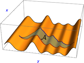
Out-of-plane acoustic modes are characteristic vibrations in graphene. These low frequency modes, seen in Fig. 1, are easy to excite and carry most of the vibrational energy Jiang2015 ; Bastos2018 . They consist in a dynamic elongation, bending and torsion of the local bonds. The stretching or tension of the bonds is by far the most important for the electrons, since it causes a greater impact on the tunneling parameter RevModPhys.81.109 . Some lattice deformations can be expressed by a gauge field using a Hamiltonian at low energies Bastos2018 ; Vozmediano2010 .

Figure 1: Random ripples of a graphene sheet. Two possible electron paths which enclose the area $\mathcal{A}$ are indicated.

The low-energy Hamiltonian for non-interacting electrons in deformed graphene for flexural deformations has been investigated qualitatively and quantitatively in the literature Morpurgo_2006 ; Guinea2009 ; Rainis_Guinea_2011 ; Bastos2018 ; Sasaki2008 . It consists in a Dirac equation added with pseudoelectromagnetic effective fields plus additional contributions caused by several mechanisms, as for example, a $\pi-\sigma$ band hybridization (proportional to the curvature of graphene flake). Other effects of electron-flexural phonons coupling in graphene have been disscused in the literature Ocha_2012 . Also, we need to take into account interactions with the substrate. Let us write first the contribution from the pseudoelectromagnetic fields, this is given by Morpurgo_2006 ; Guinea2009 ; Rainis_Guinea_2011 ,

$$\mathcal{\hat{H}}_{\eta}(\bm{r})=v_{F}\bm{\sigma}_{\eta}\cdot\left(\bm{\hat{p}}-\eta\bm{A}(\bm{r},t)\right)+V(\bm{r},t)\sigma_{0},$$ (1)

where $\bm{r}=(x,y)$ is the position vector, the subscript $\eta=\pm 1$ labels the Dirac points $\bm{K},\bm{K}\,^{\prime}$ respectively; $v_{F}$ is the Fermi velocity ($v_{F}/c\approx 1/300$ with $c$ is the vacuum speed of light); $\bm{\hat{p}}=(\hat{p}_{x},\hat{p}_{y})$ is the moment operator for the charge carriers, $\bm{\sigma}=(\eta\sigma_{x},\sigma_{y})$ is the Pauli matrix vector and $\sigma_{0}$ the $2\times 2$ identity matrix, and $\bm{A}$ and $V$ are the pseudo vector and scalar potentials respectively, given by Guinea2009 ; Naumis2017 ; Oliva2015 ; Bastos2018

$$V(\bm{r},t)=g(\varepsilon_{xx}+\varepsilon_{yy})$$ (2)

$$\bm{A}(\bm{r},t)=(A_{x},A_{y})=\frac{\hbar\beta}{2a_{cc}}(\varepsilon_{xx}-\varepsilon_{yy},-2\varepsilon_{xy})$$ (3)

The parameter $a_{cc}=1{.}42$ Å is the interatomic distance for undeformed graphene lattice and the dimensionless coefficient $\beta\approx 3{.}0$ measures the effect of the deformation on the hopping parameter. The coupling $g$ was thought first to be aroundVozmediano2010 $20$ eV , however, this turned out to be a bare estimation as charge screening leads to a much lower renormalized value katsnelson_2020 $g\approx 4$ eV. The coefficient $g$ refers to flexural changes in the membrane while the term ${\hbar\beta}/{2a_{cc}}$ refers to changes in bond length, as we know it requires more energy to make bond length changes to a rearrangement in the positions of the atoms on the membrane Suzuura2002 . Therefore, depending on the deformation, the value of $g$ is within a range of energies while the factor ${v_{F}\hbar\beta}/{2a_{cc}}\approx{6.932}$ eV remains approximately constant (within the validity range of our model).

In general, we can consider a displacement outside the plane $h=h(\bm{r},t)$, and a displacement inside the plane $\bm{u}=\bm{u}(\bm{r},t)$. The stress tensor $\varepsilon_{\mu\nu}$ is given by

$$\varepsilon_{\mu\nu}=\frac{1}{2}\left(\partial_{\mu}h\partial_{\nu}h\right)+\frac{1}{2}\left(\partial_{\mu}u_{\nu}+\partial_{\nu}u_{\mu}\right),\,\,\,\mu,\nu=x,y.$$ (4)

We shall consider the simplest case, in which the deformation is only perpendicular to the plane, i.e., $\bm{u}=0$, so from Eq. (4)

$$\begin{split}\varepsilon_{xx}&=\frac{1}{2}\left(\partial_{x}h\right)^{2}\\ \varepsilon_{yy}&=\frac{1}{2}\left(\partial_{y}h\right)^{2}\\ \varepsilon_{xy}&=\frac{1}{2}\left(\partial_{x}h\right)\left(\partial_{y}h\right)\end{split}$$ (5)

We now discuss whether to include or not corrections to Eq. (1) depending on the experimental scenario. Out of plane hybridize $\pi$ orbitals with higher orbitals of carbon, leading to a first-order contribution in the spin-orbit interaction strength, contrary to in-plane distortions, whose contribution is at least quadratic Ocha_2012 . The corrections to the Hamiltonian are given by Ocha_2012 ,

$$\mathcal{\hat{H}}=\mathcal{\hat{H}}_{A_{1}}+\mathcal{\hat{H}}_{B_{2}}+\mathcal{\hat{H}}_{G^{\prime}}$$ (6)

where the labels $A_{1},B_{2},G^{\prime}$ are the irreducible representations of the group $C_{6}^{"}$, resulting from considering a graphene’s unit cell with six atoms, used in such a way to avoid dealing with degenerate states at two inequivalent Dirac points Ocha_2012 . Such corrections leads to a Kane-Mele mass and a Rashba-like coupling present only in the case of a mirror symmetry breaking. Both coupling effects are weak Morpurgo_2006 ; Ocha_2012 , as the estimates are in the range of $1-15$ $\mu$eV. , for the present work such effects can be safely neglected as a first approximation.

Also, the $\sigma-\pi$ orbitals hybridization leads to a correction to $V(\bm{r})$ as we need to add in the diagonal of the Dirac equation the following potential, Kim_2008 ; Rainis_Guinea_2011 ,

$$V_{\pi\sigma}(\bm{r})=-g_{1}(\nabla^{2}h)^{2}$$ (7)

where $g_{1}=3\alpha/4a_{cc}$ and $\alpha\approx 9.23$ eV. The resulting $V_{\pi\sigma}(\bm{r})$ from local curvature will off-set the charge neutrality point from the average chemical potential Kim_2008 .

In the same line of reasoning, a substrate flexural deformations would be accompanied by the variation of on-site energies of carbon orbitals. This can be treated by decomposing the interaction into a smooth spatial effective potentialRainis_Guinea_2011 $V_{sub}(\bm{r})\sigma_{0}$ and, if the substrate is such that produces a bipartite symmetry breaking, an extra termMorpurgo_2006 $\Delta(\bm{r})\sigma_{z}=V_{A}(\bm{r})-V_{B}(\bm{r})\sigma_{z}$, which measures the difference of the electrostatic potential in the two sublattices $A$ and $B$, for example, due to charges located at random position in the substrate supporting graphene. The inclusion of this term depends upon the kind of substrate, for example, in SiO₂ such component can be neglected as graphene follows the substrate potential in a coarse-grained and smooth manner Morpurgo_2006 or in graphene over oxidized Cu (111) surface Gottardi2015 . For simplicity, here we will consider substrates in which the local potential $\Delta(\bm{r})\sigma_{z}$ can be neglected. Therefore, the hybridization and substrate effects can be taken into account by making the following replacement in Eq. (1),

$$V(\bm{r},t)\rightarrow V(\bm{r},t)+V_{sub}(\bm{r},t)+V_{\pi\sigma}(\bm{r},t)$$ (8)

For certain substrates as oxidized Cu (111) surface, a high-k dielectric material, the alteration of graphene due to electrostatic effects is minimal and in fact $V_{sub}(\bm{r},t)$ can be neglected Gottardi2015 .

To simplify the resulting equations, we introduce new variables defined as,

$$\begin{split}l_{1}(\bm{r},t)&\equiv\left(\partial_{x}h\right)^{2}-\left(\partial_{y}h\right)^{2}\\ l_{2}(\bm{r},t)&\equiv 2\left(\partial_{x}h\right)\left(\partial_{y}h\right)\end{split}$$ (9)

which will give us information about how “strong" the vertical displacements are. On the other hand, by making use of the Eqs. (2), (3),(5) and (9), we can rewrite the scalar and pseudo-vector potentials,

$$\begin{split}V(\bm{r},t)&=\frac{g}{2}\sqrt{l_{1}^{2}(\bm{r},t)+l_{2}^{2}(\bm{r},t)}\\ \bm{A}(\bm{r},t)&=\frac{\hbar\beta}{4a_{cc}}\left[l_{1}(\bm{r},t)\hat{x}-l_{2}(\bm{r},t)\hat{y}\right].\end{split}$$ (10)

From Eq. (1) and (10), the Hamiltonian is

$$\bm{\mathcal{\hat{H}}}_{\eta}(\bm{r})=\bm{\mathcal{\hat{H}}}_{0}(\bm{r})+\bm{W}(\bm{r},t)+V_{eff}(\bm{r},t)\sigma_{0}$$ (11)

with,

$$V_{eff}(\bm{r},t)=\left(\frac{g}{2}|l(\bm{r},t)|-g_{1}(\nabla^{2}h)^{2}\right)$$ (12)

The hat is used to denote the differential operators,

$$\begin{split}\bm{\mathcal{\hat{H}}}_{0}(\bm{r})&=v_{F}\left(\begin{array}[]{lcc}0&(\eta\hat{p}_{x}-i\hat{p}_{y})\\ \eta\hat{p}_{x}+i\hat{p}_{y}&0\end{array}\right)\\ \bm{W}(\bm{r},t)&=\left(\begin{array}[]{lcc}0&-\eta\tilde{\beta}l(\bm{r},t)\\ -\eta\tilde{\beta}l^{*}(\bm{r},t)&0\end{array}\right)\end{split}$$ (13)

where $l(\bm{r},t)\equiv\eta l_{1}(\bm{r},t)+il_{2}(\bm{r},t)$ and we defined the parameter $\bar{\beta}$ as,

$$\bar{\beta}=\frac{v_{F}\hbar\beta}{4a_{cc}}\approx 3.476\text{ eV}$$ (14)

The dynamic equation for the spinor $\Psi_{\eta}(\bm{r},t)$ follows a time-dependent Schrödinger type equation

$$\begin{split}i\hbar\frac{\partial}{\partial t}\Psi_{\eta}(\bm{r},t)=\bm{\mathcal{\hat{H}}}_{\eta}(\bm{r})\Psi_{\eta}(\bm{r},t)\end{split}$$ (15)

where

$$\Psi_{\eta}(\bm{r},t)=\left(\begin{array}[]{cc}\psi_{A}^{\eta}(\bm{r},t)\\ \psi_{B}^{\eta}(\bm{r},t)\end{array}\right)$$ (16)

It is straightforward to prove that the Schrödinger type equation (15) can be rewritten as

$$\begin{split}i\hbar\frac{\partial\psi_{A}^{\eta}}{\partial t}&=V_{eff}(\bm{r},t)\psi_{A}^{\eta}+\left[v_{F}(\eta\hat{p}_{x}-i\hat{p}_{y})-\eta\bar{\beta}l\right]\psi_{B}^{\eta},\\ i\hbar\frac{\partial\psi_{B}^{\eta}}{\partial t}&=V_{eff}(\bm{r},t)\psi_{B}^{\eta}+\left[v_{F}(\eta\hat{p}_{x}+i\hat{p}_{y})-\eta\bar{\beta}{l^{*}}\right]\psi_{A}^{\eta}.\\ \end{split}$$ (17)

Notice how the magnitude of the disorder enters in the Dirac equation through the parameters $\bar{\beta}$ and $g$. While $g$ plays the role of a random local chemical potential, $\tilde{\beta}$ is a random local magnetic field.

Eq. (17) is a complex stochastic equation. Instead of solving the time-dependent problem, we consider that the deformation process is adiabatic in the time scale of the electron dynamics. In such a case, we can suppose that the disorder is quenched and thus $l_{1}$ and $l_{2}$ are time-independent. In such a case, Eq. (13) becomes a time-independent Hamiltonian with a spatial random potential $l(\bm{r},t)=l(\bm{r})$. This is the case of topographic corrugations, such as wrinkles and foldings Wei2018 ; Verhagen2019 .

Returning to Eq. (15) becomes the time-independent Schrödinger equation $\bm{\mathcal{\hat{H}}}_{\eta}(\bm{r})\Psi_{\eta}(\bm{r})=E\Psi_{\eta}(\bm{r})$ and we are interested in finding the distribution of the Hamiltonian eigenvalues of $\bm{\mathcal{\hat{H}}}_{\eta}(\bm{r})$ and the wavefunctions.

III Folded Deformations

To understand the changes induced by random flexural deformations, we study folded deformations. Such kind of fields have been observed experimentally in deformed graphene Kim2011 ; YI2016 ; Hallam2015 and there are some studies for particular deformations RCarrillo2016 ; Nancy2018 ; Sandler2018 . In a general folded deformation, the field does not vary in one direction. Therefore, it can be written as,

$$h(y)=\sum_{k=-k_{c}}^{k_{c}}a_{k}\exp(iky)$$ (18)

with $a_{-{k}}=a_{{k}}^{*}$ as $h({y})$ is a real, and the coefficients $a_{{k}}$ can be deterministic or random variables. $k_{c}$ is a cutoff parameter and in what follows all sums are understood to use it. $k_{c}$ can be estimated from the Bose-Einstein distribution and depends upon the experimental conditions (see Appendix A).

From Eqs. (3) and (4) , the vectorial potential has only one component different from zero,

$$A_{x}(y)=\frac{\hbar\beta}{4a_{cc}}\left[\sum_{k}a_{k}k\exp(iky)\right]^{2}$$ (19)

The advantage of this particular deformation is that $\bm{A}(\bm{r})$ is in the Coulomb gauge, as it satisfies $\nabla\cdot\bm{A}(\bm{r})=0$, therefore can be obtained as the derivative of a scalar field,

$$A_{i}=\epsilon_{ij}\partial_{j}\Phi(\bm{r})$$ (20)

where $\epsilon_{ij}$ is the 2D Levi-Civita tensor with $i=x,y$ and $j=x,y$. For this particular case, we express $\Phi(y)$ in terms of the following Fourier decomposition,

$$\Phi(y)=\Phi_{0}(y)+\sum_{k\neq 0}e^{iky}\tilde{\Phi}(k)$$ (21)

with,

$$\Phi_{0}(y)=\frac{\hbar\beta}{4a_{cc}}\left(\sum_{k}k^{2}|a_{k}|^{2}\right)y$$ (22)

and,

$$\tilde{\Phi}(k)=-i\frac{\hbar\beta}{4a_{cc}k}\left[\sum_{k^{\prime}}a_{k}a_{k^{\prime}-k}^{*}k^{\prime}\left(k^{\prime}-k\right)\right]$$ (23)

The associated pseudomagnetic field is $\bm{B}=\bm{\nabla}^{2}\Phi(\bm{r})$. It is worthwhile noticing that although $\Phi_{0}(y)$ does not produce a pseudomagnetic field, it produces an Aharonov-Bohm like effect as it leads to a constant $\bm{A}(\bm{r})$. Finally, the contribution from the $\sigma_{0}$ term is,

$$V_{eff}(y)=\frac{g}{2}|l_{1}(y)|-\frac{g_{1}}{4|l_{1}(y)|}\left(\frac{\partial|l_{1}(y)|}{\partial y}\right)^{2}$$ (24)

with $l_{1}(y)=v_{F}A_{x}(y)/\bar{\beta}$.

An interesting consequence of having a field derived from the potential is that for any flexural field, being deterministic or random, the zero-mode can always be constructed. Zero modes in the Dirac equation are topologically protected thus their existance is independent of $V_{eff}(y)$. As a consequence, the usual approach is to neglect such contribution keeping only the pseudomagnetic field katsnelson_2020 . Also, the contribution from $g$ and $g_{1}$ tends to cancel each. Therefore, from the Schrödinger and Eq. (20), we obtain that for $E=0$ the wave function is,

$$\psi_{\pm}(\bm{r})=(const.)(1\pm\sigma_{z})\left(\begin{array}[]{c}e^{\Phi(y)}\\ e^{-\Phi(y)}\end{array}\right)$$ (25)

where $\sigma_{z}$ is the Pauli $z$ matrix. Similar functions were studied years ago in the context of the integer quantum Hall transition Andreas1994 . It can be proved that for a random magnetic field in which the vector potential satisfies a Gaussian white-noise distribution with mean zero and variance $\Delta_{A}$ such that the average coefficients in Eq. (21) are,

$$\langle\tilde{\Phi}(k)\tilde{\Phi}(k^{\prime})\rangle=(2\pi)^{2}\delta(k-k^{\prime})\frac{\Delta_{A}}{k^{2}}$$ (26)

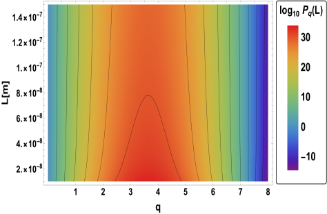
while the resulting wave-function is multifractal Andreas1994 . In a sample of size $L\times L$, the moments of the participation ratio $P_{q}(L)$ that measures a multifractal localization Barrios_Vargas_2012 ,

$$P_{q}(L)=\langle|\psi({\bm{r})}|^{2q}\rangle$$ (27)

are given by Andreas1994 ,

$$P_{q}(L)\approx\frac{1}{L^{2+\tau(q)}}$$ (28)

with,

$$\tau(q)=2(q-1)+\frac{\Delta_{A}}{\pi}q(1-q)$$ (29)

where $q$ need not be integer. In Fig. 3 we present a surface plot of $P_{q}(L)$ for a $\Delta_{A}$ below the quantum phase transition that occurs at $\Delta_{A}=\pi$. For big samples, the multifractal spectrum is dominated by its maximal value, from where the typical participation is Andreas1994 ,

$$P_{\text{typical}}(L)=e^{\langle\ln|\Psi|^{2}\rangle}\approx\frac{1}{L^{2+\Delta_{A}/\pi}}$$ (30)

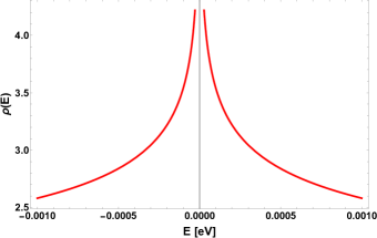
Around these states and near the Fermi energy, the density of states (DOS) is Andreas1994 ,

$$\rho(E)=E^{\frac{2-z}{z}}$$ (31)

with $z=2+\Delta_{A}/\pi$. Fig. 2 presents the resulting DOS showing that the main effect is an incresead density at the Dirac point. The wavefunction multifractality and the power law DOS means that an unusual electron velocity distribution will appear even in the simplest case of a Gaussian random flexural field, without restoring to Levy distributions of membrane jumps in graphene. In any case, the Levy jumps will induce an even more unusual distribution.

Figure 2: Multifractality of zero modes wave functions. Contour plot of $P_{q}(L)$ as a function of the sample length $L$ and the exponent $q$, for $\Delta_{A}=1$, chosen to be below the quantum phase transition to the Hall effect at $\Delta_{A}=\pi$.

.

We end up by considering the particular contribution of the Aharonov-Bohm term which for some geometries produces interesting effects in graphene deJuan2011 , nevertheless has not been studied for random fields. First we write the Fourier coefficients $a_{k}$ as the sum of an average plus a fluctuation part, $a_{k}=\langle a_{k}\rangle+\delta a_{k}$. If $a_{k}$ is Gaussian distributed with zero mean we have,

$$\Phi_{0}(y)=\frac{\hbar\beta}{4a_{cc}}\sum_{k}(\delta a_{k})^{2}k^{2}y\approx\frac{\pi}{6}\frac{\hbar\beta}{a_{cc}}\Delta_{A}k_{c}^{3}y$$ (32)

and thus the phase difference between particles, with the same start and end points, but travelling along two different paths is,

$$\Delta\mathcal{\phi}=\left(\frac{d\Phi_{0}(y)}{dy}\mathcal{A}\right)\frac{e}{\hbar}=\frac{\pi}{6}\frac{\beta}{a_{cc}}(\Delta_{A}k_{c}^{3}\mathcal{A})e$$ (33)

where $\mathcal{A}$ is the area bounded by the two paths as seen in Fig. 1. For thermally activated fields, $k_{c}$ is determined from the temperature ($T$) population given by the Bose-Einstein distribution. As $\Delta_{A}\sim k_{B}T$, Eq. (33) implies a very strong temperature dependent phase shift. This result is in agreement with recent first-principles calculations based on density functional theory and the Boltzmann equationTue_2020 .

Figure 3: Density of states (DOS) as a function of the energy and around the Dirac point with added random pseudomagnetic fields, with $\Delta_{A}=1$, chosen to be below the quantum phase transition to the Hall effect at $\Delta_{A}=\pi$.

.

IV Conclusions.

We studied the effects in the electronic properties of graphene of folded flexural deformations, which are equivalent to electromagnetic fields in the Columb gauge. First we studied general folded deformations giving an expression for the zero-modes which are the ones at the Fermi level for half-filled systems. For random Gaussian distributed folded deformations, we made contact with works on the quantum Hall effect under random magnetic fields, showing that the wave functions are multifractal and the density of states has a power law behavior. This indicates that the system can present interesting behaviors. In particular, there is a remarkable Aharonov-Bohm pseudo-effect. The wavefunction multifractality can be observed as an unusual dependence of the conductance with the length or by an unusual electron velocity distribution, as has been observed in some experiments Ackerman2016 . In fact, there are clear signatures of such zero modes exotic multifractal conductance fluctuations in recent experiments with high-mobility single-layer graphene field-effect transistors Amin2018 .

Data Availability

The data that support the findings of this study are available from the corresponding author upon reasonable request.

Appendix A Cut-off criteria for the deformation field

Consider the displacement outside the plane, in general it can be written as,

$$h(\bm{r})=\sum_{\bm{k=-k_{c}}}^{kc}a_{\bm{k}}\exp(i\bm{kr})$$ (34)

It is important to remark that for graphene, the room temperature is far below the Debye temperature Feng2018 ; Balandin2020 , which is about $1000$ and $2300$ K , and therefore $\hbar\omega(k_{c})\leq k_{B}T$. As the purely harmonic flexural dispersion goes as Castro_2010 $\omega(\bm{k})=\alpha|\bm{k}|^{2}$ with $\alpha=4.6^{2}m^{2}/s$, it follows that,

$$|\bm{k}_{c}|\approx\sqrt{\frac{k_{B}T}{\alpha\hbar}}$$ (35)

Notice that $k_{c}$ is a strain dependent quantity Castro_2010 ; Zakharchenko_2010 . In fact, for free-standing graphene at thermal equilibrium,

$$\left\langle a_{\bm{k}}^{2}\right\rangle=\frac{\hbar(1+2n_{B}(\omega(\bm{k})))}{2M_{C}\omega(\bm{k})}\approx\frac{k_{B}T}{M_{C}\omega(\bm{k})}$$ (36)

where $n_{B}(\omega(\bm{k}))$ is the thermal population of mode $\bm{k}$, $M_{C}$ is the carbon mass and the second equality holds when $\hbar\omega(\bm{k})\ll k_{B}T$. For purely harmonic flexural modes the fluctuation $\langle a_{\bm{k}}^{2}\rangle$ diverges as $|\bm{k}|^{-4}$ for small $\bm{k}$. In real samples, however, it is known that the singularity gets renormalized due to lattice imperfections (i.e., by anharmonic effects). The resulting dispersion can be parametrized as $\omega(k)=\alpha\sqrt{k^{4}+k^{4-\tau}k_{c}^{\tau}}$ for $\tau>0$, from where it follows that the quadratic mean displacement of each field mode, in the long wavelenght, is given by Fratini2013 ,

$$\langle|a_{k}|^{2}\rangle\propto\frac{k_{B}T}{k^{4-\tau}k_{c}^{\tau}}$$ (37)

where $\tau$ depend on the physical mechanism of renormalization. The physical scenarios are Fratini2013 : a) substrate pinning that opens a gap in the phonon spectrum, corresponding to $\tau=4$; b) strain which makes the dispersion linear at long wavelengths, $\tau=2$, c) anharmonic effects which yield $\tau=0{.}82$.

Appendix B Coulomb norm for general pseudo-electromagnetic fields

Although some works assume the Coulomb norm for general pseudo-electromagnetic fields Kailasvuori_2009 , let us show that in general such deformation can not be written as the derivative of a scalar field. This can be proved as follows, if we consider $A_{i}(\bm{r})=\epsilon_{ij}\partial_{j}\Phi(\bm{r})$ with $\Phi(\bm{r})=\sum_{\bm{k}}b_{\bm{k}}\exp(i\bm{k}\cdot\bm{r})$ it holds that

$$\begin{split}b_{\bm{k}}&=-\frac{iv_{F}\tilde{\beta}}{k_{y}}\sum_{\bm{k}^{\prime}}a_{\bm{k}}a_{\bm{k}^{\prime}}^{*}(k_{x}k_{x}^{\prime}-k_{y}k_{y}^{\prime})e^{-i\bm{k}^{\prime}\cdot\bm{r}}\\ \text{and }b_{\bm{k}}&=-\frac{iv_{F}\tilde{\beta}}{k_{x}}\sum_{\bm{k}^{\prime}}a_{\bm{k}}a_{\bm{k}^{\prime}}^{*}(k_{x}k_{y}^{\prime}+k_{y}k_{x}^{\prime})e^{-i\bm{k}^{\prime}\cdot\bm{r}}.\end{split}$$ (38)

In general, the system of equations in Eq. (38) has no solutions for $b_{\bm{k}}$ except for few particular cases, as the folded potential studied here.

References

- [1] K. S. Novoselov, A. K. Geim, S. V. Morozov, D. Jiang, Y. Zhang, S. V. Dubonos, I. V. Grigorieva, and A. A. Firsov. Science, 306(5696):666–669, 2004.
- [2] Alessandro Cresti, Norbert Nemec, Blanca Biel, Gabriel Niebler, François Triozon, Gianaurelio Cuniberti, and Stephan Roche. Nano Research, 1(5):361–394, 2008.
- [3] L.E.F.F. Torres, S. Roche, and J.C. Charlier. Introduction to Graphene-Based Nanomaterials: From Electronic Structure to Quantum Transport. Introduction to Graphene-based Nanomaterials: From Electronic Structure to Quantum Transport. Cambridge University Press, 2014.
- [4] A. H. Castro Neto, F. Guinea, N. M. R. Peres, K. S. Novoselov, and A. K. Geim. Rev. Mod. Phys., 81:109–162, Jan 2009.
- [5] S. Das Sarma, Shaffique Adam, E. H. Hwang, and Enrico Rossi. Rev. Mod. Phys., 83:407–470, May 2011.
- [6] Gerardo G Naumis, Salvador Barraza-Lopez, Maurice Oliva-Leyva, and Humberto Terrones. Reports on Progress in Physics, 80(9):096501, aug 2017.
- [7] G. G. Naumis, M. Terrones, H. Terrones, and L. M. Gaggero-Sager. Applied Physics Letters, 95(18):182104, 2009.
- [8] D. S. Díaz-Guerrero, I. Rodríguez-Vargas, G. G. Naumis, and L. M. Gaggero-Sager. Fractals, 24(02):1630002, 2016.
- [9] G.P. Zhang and Z.J. Qin. Physics Letters A, 374(40):4140 – 4143, 2010.
- [10] G.P. Zhang and Z.J. Qin. Chemical Physics Letters, 516(4):225 – 229, 2011.
- [11] M. A. H. Vozmediano, M. I. Katsnelson, and F. Guinea. Physics Reports, 496(4):109–148, 2010.
- [12] M. Oliva-Leyva and Gerardo G. Naumis. Phys. Rev. B, 88:085430, Aug 2013.
- [13] M. Oliva-Leyva and Gerardo G. Naumis. Physics Letters A, 379(40):2645–2651, 2015.
- [14] F. Guinea. Solid State Communications, 152(15):1437–1441, 2012.
- [15] B. Amorim, A. Cortijo, F. de Juan, A. G. Grushin, F. Guinea, A. Gutiérrez-Rubio, H. Ochoa, V. Parente, R. Roldán, P. San-Jose, J. Schiefele, M. Sturla, and M. A. H. Vozmediano. Physics Reports, 617:1–54, 2016.
- [16] R. Carrillo-Bastos, D. Faria, A. Latgé, F. Mireles, and N. Sandler. Phys. Rev. B, 90:041411, Jul 2014.
- [17] Chen Si, Zhimei Sun, and Feng Liu. Nanoscale, 8(6):3207–3217, 2016.
- [18] Deji Akinwande, Christopher J. Brennan, J. Scott Bunch, Philip Egberts, Jonathan R. Felts, Huajian Gao, Rui Huang, Joon-Seok Kim, Teng Li, Yao Li, Kenneth M. Liechti, Nanshu Lu, Harold S. Park, Evan J. Reed, Peng Wang, Boris I. Yakobson, Teng Zhang, Yong-Wei Zhang, Yao Zhou, and Yong Zhu. Extreme Mechanics Letters, 13:42–77, 2017.
- [19] G. E. Volovik and M. A. Zubkov. Annals of Physics, 340(1):352–368, 2014.
- [20] G. E. Volovik and M. A. Zubkov. Annals of Physics, 356:255–268, 2015.
- [21] Richard Kerner, Gerardo G. Naumis, and Wilfrido A. Gómez-Arias. Physica B: Condensed Matter, 407(12):2002–2008, 2012.
- [22] M. Oliva-Leyva and Gerardo G. Naumis. Phys. Rev. B, 93:035439, Jan 2016.
- [23] Ramon Carrillo-Bastos and Gerardo G. Naumis. physica status solidi (RRL) – Rapid Research Letters, 12(9):1800072, 2018.
- [24] E. McCann, K. Kechedzhi, Vladimir I. Fal’ko, H. Suzuura, T. Ando, and B. L. Altshuler. Weak-localization magnetoresistance and valley symmetry in graphene. Phys. Rev. Lett., 97:146805, Oct 2006.
- [25] K. Kechedzhi, O. Kashuba, and Vladimir I. Fal’ko. Quantum kinetic equation and universal conductance fluctuations in graphene. Phys. Rev. B, 77:193403, May 2008.
- [26] Kazi Rafsanjani Amin, Samriddhi Sankar Ray, Nairita Pal, Rahul Pandit, and Aveek Bid. Exotic multifractal conductance fluctuations in graphene. Communications Physics, 1(1):1, Feb 2018.
- [27] M. Neek-Amal, P. Xu, J. K. Schoelz, M. L. Ackerman, S. D. Barber, P. M. Thibado, A. Sadeghi, and F. M. Peeters. Nature Communications, 5(1):4962, 2014.
- [28] M. L. Ackerman, P. Kumar, M. Neek-Amal, P. M. Thibado, F. M. Peeters, and Surendra Singh. Phys. Rev. Lett., 117:126801, Sep 2016.
- [29] P. Xu, M. Neek-Amal, S. D. Barber, J. K. Schoelz, M. L. Ackerman, P. M. Thibado, A. Sadeghi, and F. M. Peeters. Nature Communications, 5(1):3720, 2014.
- [30] Dimitri Volchenkov, Yue Kai, Wenlong Xu, Bailin Zheng, Nan Yang, Kai Zhang, and P. M. Thibado. Complexity, 2019:6101083, 2019.
- [31] Jinhai Mao, Slaviša P. Milovanović, Miša Anđelković, Xinyuan Lai, Yang Cao, Kenji Watanabe, Takashi Taniguchi, Lucian Covaci, Francois M. Peeters, Andre K. Geim, Yuhang Jiang, and Eva Y. Andrei. Nature, 584(7820):215–220, 2020.
- [32] Y. Wu, D. Zhai, C. Pan, B. Cheng, T. Taniguchi, K. Watanabe, N. Sandler, and M. Bockrath. Nano Letters, 18(1):64–69, 01 2018.
- [33] Christine A. Muschik, Simon Moulieras, Adrian Bachtold, Frank H. L. Koppens, Maciej Lewenstein, and Darrick E. Chang. Phys. Rev. Lett., 112:223601, Jun 2014.
- [34] Eduardo V. Castro, H. Ochoa, M. I. Katsnelson, R. V. Gorbachev, D. C. Elias, K. S. Novoselov, A. K. Geim, and F. Guinea. Phys. Rev. Lett., 105:266601, Dec 2010.
- [35] Jonas R. F. Lima, Luiz Felipe C. Pereira, and Anderson L. R. Barbosa. Phys. Rev. E, 99:032118, Mar 2019.
- [36] Tianli Feng and Xiulin Ruan. Phys. Rev. B, 97:045202, Jan 2018.
- [37] Alexander A. Balandin. ACS Nano, 14(5):5170–5178, May 2020.
- [38] Ikuo. Ichinose. Modern Physics Letters A, 17(21):1355–1365, 2020/08/04 2002.
- [39] Mehrshad Mehboudi, Kainen Utt, Humberto Terrones, Edmund O Harriss, Alejandro A Pacheco SanJuan, and Salvador Barraza-Lopez. Proceedings of the National Academy of Sciences of the United States of America, 112(19):5888–5892, 05 2015.
- [40] Jinying Wang, Shibin Deng, Zhongfan Liu, and Zhirong Liu. National Science Review, 2(1):22–39, 01 2015.
- [41] T. O. Wehling, A. M. Black-Schaffer, and A. V. Balatsky. Advances in Physics, 63(1):1–76, 01 2014.
- [42] Jin-Wu Jiang, Bing-Shen Wang, Jian-Sheng Wang, and Harold S Park. Journal of Physics: Condensed Matter, 27(8):083001, jan 2015.
- [43] A. F. Morpurgo and F. Guinea. Intervalley scattering, long-range disorder, and effective time-reversal symmetry breaking in graphene. Phys. Rev. Lett., 97:196804, Nov 2006.
- [44] Diego Rainis, Fabio Taddei, Marco Polini, Gladys León, Francisco Guinea, and Vladimir I. Fal’ko. Gauge fields and interferometry in folded graphene. Phys. Rev. B, 83:165403, Apr 2011.
- [45] Ken-ichi Sasaki and Riichiro Saito. Progress of Theoretical Physics Supplement, 176:253–278, 06 2008.
- [46] H. Ochoa, A. H. Castro Neto, V. I. Fal’ko, and F. Guinea. Spin-orbit coupling assisted by flexural phonons in graphene. Phys. Rev. B, 86:245411, Dec 2012.
- [47] Mikhail I. Katsnelson. The Physics of Graphene. Cambridge University Press, 2 edition, 2020.
- [48] Hidekatsu Suzuura and Tsuneya Ando. Phys. Rev. B, 65:235412, May 2002.
- [49] Eun-Ah Kim and A. H. Castro Neto. Graphene as an electronic membrane. EPL (Europhysics Letters), 84(5):57007, dec 2008.
- [50] Stefano Gottardi, Kathrin Müller, Luca Bignardi, Juan Carlos Moreno-López, Tuan Anh Pham, Oleksii Ivashenko, Mikhail Yablonskikh, Alexei Barinov, Jonas Björk, Petra Rudolf, and Meike Stöhr. Comparing graphene growth on cu(111) versus oxidized cu(111). Nano Letters, 15(2):917–922, Feb 2015.
- [51] Yujie Wei and Ronggui Yang. Nanomechanics of graphene. National Science Review, 6(2):324–348, 06 2018.
- [52] Tim Verhagen, Barbara Pacakova, Milan Bousa, Uwe Hübner, Martin Kalbac, Jana Vejpravova, and Otakar Frank. Superlattice in collapsed graphene wrinkles. Scientific Reports, 9(1):9972, Jul 2019.
- [53] Kwanpyo Kim, Zonghoon Lee, Brad D. Malone, Kevin T. Chan, Benjamín Alemán, William Regan, Will Gannett, M. F. Crommie, Marvin L. Cohen, and A. Zettl. Phys. Rev. B, 83:245433, Jun 2011.
- [54] Chenglin Yi, Xiaoming Chen, Liuyang Zhang, Xianqiao Wang, and Changhong Ke. Extreme Mechanics Letters, 9:84 – 90, 2016.
- [55] Toby Hallam, Amir Shakouri, Emanuele Poliani, Aidan P. Rooney, Ivan Ivanov, Alexis Potie, Hayden K. Taylor, Mischa Bonn, Dmitry Turchinovich, Sarah J. Haigh, Janina Maultzsch, and Georg S. Duesberg. Nano Letters, 15(2):857–863, 2015. PMID: 25539448.
- [56] R. Carrillo-Bastos, C. León, D. Faria, A. Latgé, E. Y. Andrei, and N. Sandler. Phys. Rev. B, 94:125422, Sep 2016.
- [57] Johannes C Rode, Dawei Zhai, Christopher Belke, Sung J Hong, Hennrik Schmidt, Nancy Sandler, and Rolf J Haug. 2D Materials, 6(1):015021, dec 2018.
- [58] Andreas W. W. Ludwig, Matthew P. A. Fisher, R. Shankar, and G. Grinstein. Phys. Rev. B, 50:7526–7552, Sep 1994.
- [59] J E Barrios-Vargas and Gerardo G Naumis. Journal of Physics: Condensed Matter, 24(25):255305, may 2012.
- [60] Fernando de Juan, Alberto Cortijo, María A. H. Vozmediano, and Andrés Cano. Nature Physics, 7(10):810–815, Oct 2011.
- [61] Tue Gunst, Kristen Kaasbjerg, and Mads Brandbyge. Phys. Rev. Lett., 118:046601, Jan 2017.
- [62] K. V. Zakharchenko, R. Roldán, A. Fasolino, and M. I. Katsnelson. Phys. Rev. B, 82:125435, Sep 2010.
- [63] S. Fratini, D. Gosálbez-Martínez, P. Merodio Cámara, and J. Fernández-Rossier. Phys. Rev. B, 88:115426, Sep 2013.
- [64] J. Kailasvuori. EPL (Europhysics Letters), 87(4):47008, aug 2009.