Uniform lower bounds on the dimension of Bernoulli convolutions

Abstract

In this note we present an algorithm to obtain a uniform lower bound on Hausdorff dimension of the stationary measure of an affine iterated function scheme with similarities, the best known example of which is Bernoulli convolution. The Bernoulli convolution measure $\mu_{\lambda}$ is the probability measure corresponding to the law of the random variable

$$\xi=\sum_{k=0}^{\infty}\xi_{k}\lambda^{k},$$

where $\xi_{k}$ are i.i.d. random variables assuming values $-1$ and $1$ with equal probability and $\frac{1}{2}<\lambda<1$. In particular, for Bernoulli convolutions we give a uniform lower bound $\dim_{H}(\mu_{\lambda})\geq 0.96399$ for all $\frac{1}{2}<\lambda<1$.

1 Introduction

In this note we will study stationary measures for certain types of iterated function schemes. We begin with an important example.

1.1 Bernoulli convolutions

The study of the properties of Bernoulli convolutions was greatly advanced by two influential papers of Paul Erdös from 1939 [5] and 1940 [6] and has remained an active area of research ever since. We briefly recall the definition: given $0<\lambda<1$ we can associate the Bernoulli convolution measure $\mu_{\lambda}$ on the real line corresponding to the distribution of the series

$$\xi=\sum_{k=0}^{\infty}\xi_{k}\lambda^{k}$$ (1)

where $(\xi_{k})_{k=1}^{\infty}$ are independent random variables assuming values $\pm 1$ with equal probability. Equivalently, this is the probability measure given by the weak-star limit of the measures

$$\mu_{\lambda}=\lim_{n\to+\infty}\frac{1}{2^{n}}\sum_{i_{1},\cdots,i_{n}\in\{0,1\}}\delta\left(\sum_{j=1}^{n}(-1)^{i_{j}}\lambda^{j}\right),$$

where $\delta(y)$ is the Dirac delta probability measure supported on $y$. The properties of these measures have been studied in great detail. We refer the reader to recent surveys by Gouëzel [13] and Hochman [18] for an overview of existing results.

The properties of the measure $\mu_{\lambda}$ are very sensitive to the choice of $\lambda$. For example, if $0<\lambda<\frac{1}{2}$ then $\mu_{\lambda}$ is supported on a Cantor set and is singular with respect to Lebesgue measure, but if $\lambda=\frac{1}{2}$ then the measure $\mu_{1/2}$ equals the normalized Lebesgue measure on $[-2,2]$. For $\frac{1}{2}<\lambda<1$ the situation is more subtle. In this case the measure $\mu_{\lambda}$ is supported on the closed interval $\left[-\frac{1}{1-\lambda},\frac{1}{1-\lambda}\right]$. It was conjectured by Erdös in 1940 [6], and proved by Solomyak in 1995 [35], that for almost all $\lambda\in(\frac{1}{2},1)$ (with respect to Lebesgue measure) the measure $\mu_{\lambda}$ is absolutely continuous. Recently Shmerkin [30], [31], developing the method of Hochman [17], improved this result to show that the set of $\frac{1}{2}<\lambda<1$ for which $\mu_{\lambda}$ is not absolutely continuous has zero Hausdorff dimension. On the other hand, it was shown by Erdös in [5] that this exceptional set of values is non-empty.

We will be concerned with another, though related, aspect of the Bernoulli convolutions $\mu_{\lambda}$, namely their Hausdorff dimension.

Definition 1.1.

The Hausdorff dimension of a probability measure $\mu$ is defined by

$$\dim_{H}(\mu):=\inf\{\dim_{H}(X)\mid\mbox{ $X$ is a Borel set with }\mu(X)=1\},$$ (2)

where $\dim_{H}(X)$ stands for the Hausdorff dimension of a set $X$, see Section 2.1 for definition.

Any measure $\mu$ which is absolutely continuous with respect to Lebesgue measure automatically satisfies $\dim_{H}(\mu)=1$, and therefore the result of Shmerkin implies that $\dim_{H}(\mu_{\lambda})=1$ for all but an exceptional set of parameters $\lambda$ of zero Hausdorff dimension. Furthermore, Varjú [36] recently proved a stronger result that $\dim_{H}(\mu_{\lambda})=1$ for all transcendental $\lambda$.

Therefore, it remains to consider the set of algebraic parameter values. It turned out that for certain class of algebraic numbers, namely, for the reciprocals of Pisot numbers, it is possible to compute Hausdorff dimension $\dim_{H}(\mu_{\lambda})$ explicitly, subject to computer resources. We briefly recall the definition.

Definition 1.2.

Pisot number $\beta$ is an algebraic number strictly greater than one all of whose (Galois) conjugates, excluding itself, lie strictly inside the unit circle.

The Pisot numbers form a closed subset of $\mathbb{R}$ and have Hausdorff dimension strictly less than $1$. The smallest Pisot number is $\beta_{min}=1.3247\ldots$ (a root of $x^{3}-x-1=0$).

The first progress on dimension of Bernoulli convolutions was made by Erdös in [5], where he showed that if $\lambda$ is the reciprocal of a Pisot number, then $\mu_{\lambda}$ is not absolutely continuous. Garsia [11] improved on the Erdös result by showing that $\dim_{H}(\mu_{\lambda})<1$ whenever $\lambda$ is the reciprocal of a Pisot number. This phenomenon is called dimension drop and it remains unknown whether Pisot numbers are the only numbers with this property.

Alexander and Zagier estimated $\dim_{H}(\mu_{\lambda})$ in the case that $\lambda=\frac{2}{1+\sqrt{5}}$ was the reciprocal of the Golden mean and Grabner, Kirschenhofer and Tichy [12] gave examples of explicit algebraic numbers $\lambda$, the so-called “multinacci” numbers for which the dimension drop takes place. The values they computed are amongst the smallest known values for the dimension of Bernoulli convolutions. For example, they estimated that

when $$\lambda^{3}-\lambda^{2}-\lambda-1=0, \mbox{ then }\dim_{H}(\mu_{\lambda})=0.980409319534731\ldots$$

when $$\lambda^{4}-\lambda^{3}-\lambda^{2}-\lambda-1=0, \mbox{ then }\dim_{H}(\mu_{\lambda})=0.986926474333800\ldots.$$

The technique developed in [12] has been subsequently extended to a wider class of algebraic parameter values cf. [1] and [15], however, the limitation of this method is that it requires studying each parameter value independently.

It is therefore a basic problem to get a uniform lower bound on $\dim_{H}\mu_{\lambda}$ for $\frac{1}{2}<\lambda<1$ and to identify possible dimension drops. A simplifying observation is that

$$\dim_{H}(\mu_{\lambda})\geq\dim_{H}(\mu_{\lambda^{2}})$$ (3)

and thus if suffices to get a lower bound for $\frac{1}{2}<\lambda<\frac{1}{\sqrt{2}}$.

Remark 1.3.

The inequality (3) is established, in particular, in [14, Proposition 2.1] for algebraic parameter values $\lambda$, but it is easy to see that it holds for all $\frac{1}{2}\leq\lambda\leq 1$, since for any probability measure $\mu$ we have that $\dim_{H}\mu*\mu\geq\dim_{H}\mu$.

Our first main result on the dimension of Bernoulli convolutions is a collection of piecewise-constant uniform lower bounds over increasingly finer partitions of the parameter space.

Theorem 1.4.

1. The dimension of Bernoulli convolutions $\mu_{\lambda}$ for any $\frac{1}{2}<\lambda<1$ satisfies

   $$\dim_{H}\mu_{\lambda}\geq G_{0}:=0.96399.$$

2. Moreover, the dimension of Bernoulli convolutions $\mu_{\lambda}$ is roughly bounded from below by a piecewise-constant function $G_{1}$ with $8$ intervals of continuity, $\dim_{H}\mu_{\lambda}\geq G_{1}(\lambda)$, where the values of $G_{1}$ are given in Table 1 for $0.5\leq\lambda\leq 0.8$.

3. The previous bound can be further refined. The dimension of Bernoulli convolutions $\mu_{\lambda}$ is bounded from below by a piecewise-constant function $G_{2}$ corresponding to approximately $10000$ intervals $\dim_{H}\mu_{\lambda}\geq G_{2}(\lambda)$, where the graph of the function $G_{2}$ is presented in Figure 9, with the particularly interesting region $0.5<\lambda<0.575$ presented in Figure 1.

In the proof, we derive (ii) from (iii) and (i) from (ii), rather than establishing each estimate independently. We choose to give the statement in three parts for the clarity of exposition.

Remark 1.5.

Our proof is computer assisted and these bounds are not sharp, at least in the following sense: using a finer partition of the parameter space one could obtain even better lower bounds. This of course requires more computer time.

Interval	$G_{1}$
$[0.5000,0.5037)$	$0.9900$
$[0.5037,0.5181)$	$0.9800$
$[0.5181,0.5200)$	$0.9700$
$[0.5200,0.5430)$	$0.9785$
$[0.5430,0.5451)$	$0.9639$
$[0.5451,0.5527)$	$0.9785$
$[0.5527,0.5703)$	$0.9850$
$[0.5703,0.8000)$	$0.9900$

Table 1: Values of $G_{1}$.

Figure 1: Plots of $G_{0}$, $G_{1}$ and $G_{2}$.

The behaviour of the lower bound function $G_{2}$ appears to be quite intriguing, in particular, the largest dimension drops seem to correspond to the reciprocals of the limit points of the set of Pisot numbers, see Section 3.4 for further discussion and Figure 9, for detailed plots.

To the best of our knowledge, the best result to date is due Feng and Feng [9]; they obtained a global lower bound of $\dim_{H}(\mu_{\lambda})\geq 0.9804085$. They give an alternative approach for computing a lower bound for $\dim_{H}(\mu_{\lambda})$, which uses the conditional entropy. Three years earlier Hare and Sidorov [14] showed that $\dim_{H}(\mu_{\lambda})\geq 0.82$. Their method depends on a result of Hochman and uses the fact that the dimension of $\mu_{\lambda}$ can be expressed in terms of the Garsia entropy and most advances on this problem are based on this idea.

Our approach is different to both and is rooted in connection between iterated function schemes and random processes. In addition to uniform estimates, it allows us to compute good lower bounds on $\dim_{H}(\mu_{\lambda})$ for individual values $\lambda$.

The following set of algebraic numbers, intimately related to Pisot numbers, is also extensively studied.

Definition 1.6.

A Salem number is an algebraic integer $\sigma>1$ of degree at least 4, conjugate to $\sigma^{-1}$, all of whose conjugates, excluding $\sigma$ and $\sigma^{-1}$, lie on the unit circle.

We refer to a survey by Smyth [34] for an introduction to the topic. The set of limit points of Salem numbers contains the Pisot numbers. We have computed the lower bound for the reciprocals of Salem numbers, thus providing a partial supporting evidence that there is no dimension drop for these parameter values.

Theorem 1.7.

1. For every one of the $99$ values $\frac{1}{2}<\lambda<1$ which is the reciprocal of a Salem number of degree at most $10$ one has that $\dim_{H}(\mu_{\lambda})\geq 0.98546875$. Detailed estimates are tabled in Appendix A.1.

2. One can also consider the $47$ known so called small Salem numbers $\frac{10}{13}<\lambda<1$ and show that $\dim_{H}(\mu_{\lambda})\geq 0.999453125$. Lower bounds on the dimensions of the Bernoulli convolutions for the reciprocals of small Salem numbers are presented in Appendix A.2.

Another conjecture suggests that there exists $\varepsilon>0$ such that for any $\lambda\in(1-\varepsilon,1)$ the dimension of the measure $\mu_{\lambda}$ equals $1$. In particular, Breulliard—Varjú [2] showed that there exists $\varepsilon>0$ so that $\dim_{H}(\mu_{\lambda})=1$ for $1-\varepsilon<\lambda<1$ under the assumption that the Lehmer’s conjecture holds. The Lehmer’s conjecture states that the Mahler measure of any nonzero noncyclotomic irreducible polynomial with integer coefficients is bounded below by some constant $c>1$. It implies, in particular, that there exists a smallest Salem number.

As another application of our method, we give an asymptotic for the lower bound of $\dim_{H}\mu_{\lambda}$ as $\lambda\to 1$ in Section 4. More precisely, we establish the following result.

Theorem 1.8.

There exist $c>0$ and $\varepsilon>0$ so that $\dim_{H}(\mu_{\lambda})\geq 1-c(1-\lambda)$ for $1-\varepsilon<\lambda<1.$

The Bernoulli convolutions are a special case of a far more general construction of self-similar measures, which we describe next.

1.2 Iterated function schemes with similarities

Let $k$ be fixed. Given $0<\lambda<1$ and $\bar{c}\in\mathbb{R}^{n}$, consider a collection $\mathcal{S}=\{f_{j},j=1,\ldots,k\}$ of $k$ contraction similarities defined by

$$f_{j}\colon\mathbb{R}\to\mathbb{R};\qquad f_{j}(x)=\lambda x{\color[rgb]{0,0,0}\,+\,}c_{j},\mbox{ for }1\leq j\leq k.$$

Let $\bar{p}=(p_{1},\cdots,p_{k})$ be a probability vector where $0<p_{j}<1$ and $\sum\limits_{j=1}^{k}p_{j}=1$.

Definition 1.9.

We call a triple $\mathcal{S}(\lambda,\bar{c},\bar{p})$ an iterated function scheme of similarities. We will omit the dependence on $\bar{c}$ and $\bar{p}$ in the sequel when it leads to no confusion.

Definition 1.10.

A probability measure $\mu$ is called a stationary measure for the contractions $f_{1},\cdots,f_{k}$ and the probability vector $\bar{p}$ if it satisfies

$$\mu=\sum_{j=1}^{k}p_{j}(f_{j})_{*}\mu,$$

i.e., $\int F(x)d\mu(x)=\sum\limits_{j=1}^{k}p_{j}\int F(f_{j}x)d\mu(x)$, for all bounded continuous functions $F$.

The existence and the uniqueness of stationary measures in this seting follows from the work of Hutchinson [19].

In this note we are particularly concerned with the following two systems. The first one has Bernoulli convolution as the stationary measure.

Example 1.11 (Function scheme for Bernoulli convolutions).

Given a real number $\frac{1}{2}<\lambda<1$ consider the iterated function scheme of two maps $f_{0}$, $f_{1}$ given by $f_{j}(x)=\lambda x+j$, $j=0,1$ and probability vector $\bar{p}=\left(\frac{1}{2},\frac{1}{2}\right)$. Then the stationary measure $\mu=\mu_{\lambda}$ corresponds to the distribution of the random variable

$$\sum_{k=0}^{\infty}\eta_{k}\lambda^{k},$$

where $\eta_{k}$ are i.i.d. assuming values $0$ and $1$ with equal probability. This agrees with formula (1) up to the change of variables $\xi_{k}=2\eta_{k}-1$.

Example 1.12 ($\{0,1,3\}$-system).

We can consider the contractions $f_{1},f_{2},f_{3}:\mathbb{R}\to\mathbb{R}$ defined by

$$f_{1}(x)=\lambda x,\quad f_{2}(x)=\lambda x+1,\quad f_{3}(x)=\lambda x+3,$$

and the probability vector $p=(\frac{1}{3},\frac{1}{3},\frac{1}{3})$. For the corresponding stationary measure $\mu_{\lambda}^{0,1,3}$ it is known that for almost all $\frac{1}{4}\leq\lambda\leq\frac{1}{3}$ with respect to Lebesgue measure we have

$$\dim_{H}(\mu_{\lambda}^{0,1,3})=\frac{\log 3}{\log\lambda^{-1}}$$

(this equality also holds for all $\lambda<\frac{1}{4}$) and for almost all $\frac{1}{3}\leq\lambda\leq\frac{2}{5}$ with respect to Lebesgue measure we have $\dim_{H}(\mu^{0,1,3}_{\lambda})=1$; see [20], [28].

The next theorem provides a lower bound for $\dim_{H}(\mu_{\lambda}^{0,1,3})$.

Theorem 1.13.

The dimension of the stationary measure $\mu_{\lambda}^{0,1,3}$ for the $\{0,1,3\}$-system has the lower bounds

1. For any $\lambda\in[\frac{1}{4},\frac{2}{5}]$ we have that $\dim_{H}(\mu_{\lambda}^{0,1,3})\geq G^{0,1,3}_{0}:=\min\left\{\frac{\log 3}{\log\lambda^{-1}},1\right\}-0.2.$

2. Moreover, $\dim_{H}(\mu_{\lambda})$ is bounded from below by a piecewise-continuous function

   $$G_{1}^{0,1,3}(\lambda)|_{I_{k}}=\min\left\{\frac{\log 3}{\log\lambda^{-1}},1\right\}-c_{k}$$

   with $11$ intervals of continuity $I_{k}$, $k=1,\ldots 11$ which are given in Table 2, together with the corresponding values $c_{k}$. In other words, for any $\lambda\in[\frac{1}{4},\frac{2}{5}]$

   $$\dim_{H}(\mu_{\lambda}^{0,1,3})\geq G_{1}^{0,1,3}(\lambda).$$

3. The estimate from part (ii) can be refined further. The dimension $\dim_{H}(\mu_{\lambda}^{0,1,3})$ is bounded from below by a piecewise-continuous function $G_{2}^{0,1,3}$ with approximately $10000$ intervals of continuity, $\dim_{H}(\mu_{\lambda}^{0,1,3})\geq G_{2}^{0,1,3}(\lambda)$. The graph of the function $G_{2}^{0,1,3}$ is presented in Figure 2.

Interval $I_{k}$	$c_{k}$
$[0.2500,0.2630]$	$0.0350$
$[0.2630,0.2650]$	$0.0550$
$[0.2650,0.2800]$	$0.0350$
$[0.2800,0.2820]$	$0.0650$
$[0.2820,0.2980]$	$0.0350$
$[0.2980,0.3210]$	$0.0850$
$[0.3210,0.3320]$	$0.1100$
$[0.3320,0.3350]$	$0.2000$
$[0.3350,0.3450]$	$0.1100$
$[0.3450,0.3670]$	$0.0800$
$[0.3670,0.4045]$	$0.0400$

Table 2: Table of values of $c_{k}$.

Figure 2: Plots of $G^{0,1,3}_{1}$ and $G^{0,1,3}_{2}$.

Remark 1.14.

An alternative version for (i) could be: For any $0.25<\lambda<0.4$ we have that $\dim_{H}\mu_{\lambda}^{0,1,3}\geq G_{0}^{0,1,3}(\lambda)$, where

$$G_{0}^{0,1,3}(\lambda):=\begin{cases}\frac{\log 3}{\log\lambda^{-1}}-0.11,&\mbox{ if }0.25<\lambda<0.3210;\\ \frac{\log 3}{\log\lambda^{-1}}-0.2,&\mbox{ if }0.3210<\lambda<0.3250;\\ 0.89,&\mbox{ otherwise. }\end{cases}$$

In particular, we see that the largest dimension drop seems to take place at $\lambda=\frac{1}{3}$. For this parameter value the dimension can be computed explicitly [21] following the method of [12], more precisely,

$$\dim_{H}\mu_{1/3}^{0,1,3}=0.83703915049\pm 10^{-10}.$$

As in the case of Bernoulli convolutions, the biggest dimension drops appear to correspond to the reciprocals of the limit points of hyperbolic numbers. However, in contrast to the Pisot numbers in the interval $(1,2)$, the limit set of hyperbolic numbers in the interval $\left(\frac{5}{2},4\right)$ is not very well studied. We give detailed plot of $G_{2}^{0,1,3}$ in Figure 11 and discuss its feautures in Section 3.4.

We obtain lower bounds for the Hausdorff dimension of Bernoulli convolutions and for the stationary measures of the $\{0,1,3\}$-system using the same method, which we outline in the next section.

1.3 Approach to lower bounds for Hausdorff dimension

The Hausdorff dimension of a measure is an important characteristic which is generally difficult to estimate, both numerically and analytically. We introduce two alternative characteristics of dimension type, namely, the correlation dimension and the Frostman dimension, which are easier to estimate and give a lower bound on the Hausdorff dimension. Whilst the numerical results suggest that in the case of iterated function schemes with similarities the Frostman dimension and Hausdorff dimension behave very different, the correlation dimension appear to exhibit the same dependence on parameter values as expected from the Hausdorff dimension.

To sum up, our approach is the following:

1. Replace the Hausdorff dimension with the correlation dimension or the Frostman dimension;

2. Compute the lower bound for the correlation dimension or the Frostman dimension.

1.3.1 Affine iterated function schemes with similarities

We begin by defining the correlation dimension which bounds the Hausdorff dimension from below (cf. Lemma 2.4). It has been introduced in [29] as a characteristic of dimension type. The notion was subsequently formalised by Pesin in [27], see also [4] and [33]. We will give a formal definition later in Section 2.2.

We proceed by introducing one of our main tools, a symmetric diffusion operator associated to an iterated function scheme.

Let $\mathcal{S}(\lambda,\bar{c},\bar{p})$ be an iterated function scheme of similarities. Assume that $J_{\lambda}\subset\mathbb{R}$ is an interval such that $f_{i}(J_{\lambda})\subset J_{\lambda}$ for all $i=1,\dots,k$. For the invariant measures $\mu_{\lambda}$ we have that $\mathop{\rm supp}\nolimits\mu_{\lambda}\subset J_{\lambda}$.

We say that an interval $J$ is $\lambda$-admissible for an iterated function scheme $\mathcal{S}(\lambda,\bar{c},\bar{p})$ if

$$\mbox{ Interior}(J)\supset\overline{\{x-y\mid x,y\in J_{\lambda}\}}$$ (4)

This is illustrated in Figure 3. Given a (possibly infinite) set of parameter values $\Lambda\subset[0,1]$ we say that the interval $J$ is $\Lambda$-admissible if it is an admissible interval for all $\lambda\in\Lambda$.

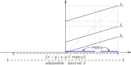
Figure 3: An iterated function scheme of three similarities $f_{0}(x)=\frac{x}{3}$, $f_{1}(x)=\frac{x}{3}+1$, and $f_{3}(x)=\frac{x}{3}+3$ and an admissible interval $J$.

Definition 1.15.

Given an iterated function scheme of similarities $\mathcal{S}(\lambda,\bar{c},\bar{p})$ for any $\alpha\in(0,1)$ we define the symmetric diffusion operator $\mathcal{D}^{(2)}_{\alpha,\mathcal{S}}$ by

$$[\mathcal{D}^{(2)}_{\alpha,\mathcal{S}}\psi](x):=\lambda^{-\alpha}\cdot\sum_{i,j=1}^{k}p_{i}p_{j}\cdot\psi\left(\frac{x-c_{i}+c_{j}}{\lambda}\right).$$ (5)

We consider this operator to be acting on the space of all functions on the real line, however the subset of nonnegative functions

$$\left\{{\color[rgb]{0,0,0}\psi}:\mathbb{R}\to\mathbb{R}^{+}\mid\mathop{\rm supp}\nolimits{\color[rgb]{0,0,0}\psi}\subseteq\overline{\{x-y\mid x,y\in J_{\lambda}\}}\right\}$$

is invariant with respect to $\mathcal{D}^{(2)}_{\alpha,\mathcal{S}}$.

Remark 1.16.

Although the difference between two operators $\mathcal{D}^{(2)}_{\alpha_{1},\mathcal{S}}$ and $\mathcal{D}^{(2)}_{\alpha_{2},\mathcal{S}}$ is in scaling factor only, we prefer to keep this factor as a part of the definition.

We are now ready to state a key result, which is the basis for our numerical method.

Theorem 1.17.

Let $\mathcal{S}(\lambda,\bar{c},\bar{p})$ be an iterated function scheme of similarities. Assume that for some $\alpha>0$ there exists an admissible compact interval $J\subset\mathbb{R}$, a function $\psi:\mathbb{R}\to\mathbb{R}^{+}$ with $\mathop{\rm supp}\nolimits\psi\subset J$ which is positive and bounded away from $0$ and from infinity on $J$, such that for any $x\in J$

$$[\mathcal{D}^{(2)}_{\alpha,\mathcal{S}}\psi](x)<\psi(x).$$ (6)

Then the correlation, and hence the Hausdorff, dimension of the $\mathcal{S}$-stationary measure $\mu$ is bounded from below by $\alpha$:

$$\dim_{H}(\mu)\geq D_{2}(\mu)\geq\alpha.$$

Theorem 1.17 allows us to obtain rigorous lower estimates for the correlation dimension $D_{2}(\mu)$ of the stationary measure $\mu$ for a single parameter value $\lambda$ (and thus for the Hausdorff dimension $\dim_{H}\mu$), once a suitable test function $\psi$ is found. This also provides us with a way to find an asymptotic lower bound and to prove Theorem 1.8.

Example 1.18.

To illustrate the way Theorem 1.17 is applied, we may choose $\lambda=0.75$, a function $\psi(x)=1-0.2|x|$ and to apply the operator $\mathcal{D}^{(2)}_{0.2,\mathcal{S}}$. It is clear that we may choose $J=[-4,4]$. Then Figure 4 shows that $\mathcal{D}^{(2)}_{0.2,\mathcal{S}}\psi(x)<\psi(x)$ and therefore $\dim_{H}\mu\geq 0.2$.

Figure 4: Image of the function $\psi=1-0.2|x|$ is strictly smaller than $\psi$.

We next want to adapt Theorem 1.17 to prepare for a computer-assisted proof of Theorems 1.4, 1.7 and 1.13. In Section 3.1 we modify the operator $\mathcal{D}^{(2)}_{\alpha,\mathcal{S}}$ to obtain an operator ${\mathcal{D}}_{\alpha,\Lambda,\mathcal{J}}$ which preserves a subspace of piecewise constant functions, and amend Theorem 1.17 so that a common test function can be used for an open set of parameter values $\Lambda=(\lambda-\varepsilon,\lambda+\varepsilon)$. This adaptation allows us to choose the test function to be piecewise constant on intervals with rational endpoints and to verify the hypothesis of Theorem 1.17 numerically, thus providing us with a means to obtain a uniform lower bound for the (correlation, and hence Hausdorff) dimension of the corresponding stationary measures.

Afterwards, in Section 3.2 we give an iterative procedure to construct a test function for the operators $\mathcal{D}^{(2)}_{\alpha,\mathcal{S}}$ and ${\mathcal{D}}_{\alpha,\Lambda,\mathcal{J}}$.

A natural question arises. Assume that $D_{2}(\mu_{\lambda})>\alpha$. Does there exist a test function $\psi$ so that (6) holds? The next result gives an affirmative answer.

Theorem 1.19.

Let $\mu_{\lambda}$ be the unique stationary measure of a scheme of contraction similarities $\mathcal{S}(\lambda)$. Then for any $\alpha<D_{2}(\mu_{\lambda})$ the hypothesis of Theorem 1.17 holds. In other words, there exists an admissible interval $J$, a piecewise constant function $\psi$ with $\mathop{\rm supp}\nolimits\psi\subset J$ which is positive and bounded away from 0 and from infinity on $J$ and such that for any $x\in J$

$$[\mathcal{D}^{(2)}_{\alpha,\mathcal{S}}\psi](x)<\psi(x).$$

As the reader will see, the technique in the proof of Theorem 1.17 exploits the fact that the maps are similarities with the same scaling coefficient. In the next section 1.3.2 we generalise the method to study other types of iterated function schemes at the expense of weaker estimates.

1.3.2 General uniformly contracting schemes

Let us denote by $B_{r}(x)$ a neighbourhood of a point $x$ of radius $r$.

We will be concerned with iterated function schemes $\mathcal{T}(\bar{f},\bar{p},J)$, where $J\subset\mathbb{R}$ is a compact interval, $\bar{f}=(f_{1},\ldots,f_{n})$ is a finite collection of uniformly contracting $C^{1+\varepsilon}$ diffeomorphisms of $\mathbb{R}$, which preserve the interval $J$, i.e. $f_{j}(J)\subset J$ for $1\leq j\leq n$ and $\bar{p}$ is a probability vector.

Following Hochman [16, §4.1], we say that the measure $\mu$ is $\alpha$-regular, if there exists a constant $C$ such that for any $r>0$ and any $x$ we have that

$$\mu(B_{r}(x))<Cr^{\alpha}.$$ (7)

One of the examples of $\alpha$-regular measures are Bernoulli convolutions [10, Proposition 2.2]. We introduce the following dimension-type characteristic of a compactly supported probability measure $\mu$ on $\mathbb{R}$, which is sometimes referred to as the Frostman dimension [8] (in the context of $\mathbb{R}^{n}$) or the lower Ahlfors dimension (in the context of general separable metric spaces). It is defined as supremum of the regularity exponents:

$$D_{1}(\mu):=\sup\{\alpha\mid\exists C:\quad\forall x,r\quad\mu\left(B_{r}(x)\right)<Cr^{\alpha}\}.$$

Remark 1.20.

We would like to warn the reader that the Frostman dimension doesn’t satisfy all conditions which a dimension of a measure is expected to satisfy, in particular, it is not closed under countable unions. We will see in Lemma 2.9 that $D_{1}(\mu)\leq D_{2}(\mu)$ for any probability measure $\mu$. It is not hard to show that it is also a lower bound for the packing dimension, as well as other dimensions which can be defined using the local dimension.

A pair of complementary results, Theorems 1.23 and 1.25 below allow one to get a lower bound on the Frostman dimension $D_{1}(\mu)$ for the stationary measure of an iterated function scheme $\mathcal{T}(\bar{f},\bar{p},J)$ in terms of an associated linear operator.

Definition 1.21.

Given an iterated function scheme $\mathcal{T}(\bar{f},\bar{p},J)$ for any $\alpha\in(0,1)$ we define the associated asymmetric diffusion operator $\mathcal{D}^{(1)}_{\alpha,\mathcal{T}}$ by

$$\mathcal{D}^{(1)}_{\alpha,\mathcal{T}}[\psi](x):=\sum_{j=1}^{n}p_{j}\cdot|(f_{j}^{-1})^{\prime}(x)|^{\alpha}\cdot\psi(f_{j}^{-1}(x)).$$ (8)

We consider this operator to be acting on the space of all functions on the real line, although it preserves nonnegative functions supported on $J$.

Remark 1.22.

Comparing (8) with (5) we see that $\mathcal{D}^{(2)}_{\alpha,\mathcal{S}}$ for Bernoulli convolution system described in Example 1.11 corresponds to the operator $\mathcal{D}^{(1)}_{\alpha,\mathcal{T}}$ for the system of three contractions

$$\mathcal{T}:=\{f_{1}(x)=\lambda x-1,f_{2}(x)=\lambda x,f_{3}(x)=\lambda x+1\}$$

and probability vector $\overline{p}=(0.25,0.5,0.25)$.

By analogy with $\mathcal{D}^{(2)}_{\alpha,\mathcal{S}}$, the operator $\mathcal{D}^{(1)}_{\alpha,\mathcal{S}}$ gives us a way to obtain a lower bound for the Frostman dimension.

We denote by $B_{r}(J)$ the closed neighbourhood of the interval $J$ of radius $r$.

Theorem 1.23.

Assume that for some $\alpha>0$ there exist $r>0$ and a function $\psi:\mathbb{R}\to\mathbb{R}_{+}$, supported on $B_{r}(J)$, positive on $B_{r}(J)$ and bounded away from $0$ and from infinity on $B_{r}(J)$, such that

$$\forall x\in B_{r}(J)\quad[\mathcal{D}^{(1)}_{\alpha,\mathcal{T}}\psi](x)<\psi(x).$$

Then the measure $\mu$ is $\alpha$–regular.

We now give a simple example to illustrate Theorem 1.23 in action.

Example 1.24.

We may consider an iterated function scheme $\mathcal{T}$ consisiting of two maps $f_{1}(x)=0.65x$ and $f_{2}(x)=0.6x+1$ with probabilities $p_{0}=p_{1}=0.5$. Then for the invariant measure $\mu$ we get $\mathop{\rm supp}\nolimits\mu\subset J=[0,2.7]$. If we choose a function $\psi(x)=1-0.4|x-1.25|$ on $J$ and apply $\mathcal{D}^{(1)}_{0.35,\mathcal{T}}$ we see that $\mathcal{D}^{(1)}_{0.35,\mathcal{T}}\psi(x)<\psi(x)$. This is illustrated in Figure 5. Therefore we conclude that the Frostman dimension of the stationary measure of this system is bounded from below by $0.35$.

Figure 5: The image of the function $\psi(x)=1-0.4|x-1.25|$ is strictly smaller than $\psi$.

As in the case of Theorem 1.19 for correlation dimension, our next result states that any lower bound can be found using this method.

Theorem 1.25.

Let $\mu$ be the stationary measure of the iterated function scheme $\mathcal{T}(\bar{f},\bar{p},J)$. Then for any $\alpha<D_{1}(\mu)$ the hypothesis of Theorem 1.23 holds. In other words there exists a neighbourhood $B_{r}(J)$ and a piecewise constant function $\psi$ with $\mathop{\rm supp}\nolimits\psi\subset B_{r}(J)$, which is positive and bounded away from 0 and from infinity on $B_{r}(J)$, and such that

$$\forall x\in B_{r}(J)\quad[\mathcal{D}^{(1)}_{\alpha,\mathcal{T}}\psi](x)<\psi(x).$$

This test function can be constructed using the process similar to the one which is used in the construction of the test function for the diffusion operator $\mathcal{D}^{(2)}_{\alpha,\mathcal{S}}$, described in §3.2.

2 Dimension of a measure

In this section we collect together some preparatory material on different dimensions of a measure and their properties. A good reference for the background reading is a book by Falconer [7]. See also the work by Mattila at al. [24] for a discussion and comparison of notions of dimension of a measure.

It is convenient to summarize some useful notation for the sequel.

For any set $X\subset\mathbb{R}$ we denote by $\mathcal{F}_{X}$ the set of real-valued positive functions, bounded away from zero and from infinity on $X$ and vanishing on $\mathbb{R}\setminus X$. We would like to equip the set of functions $\mathcal{F}_{X}$ with the partial order. We write that $f\prec g$ if $f(x)<g(x)$ for all $x\in X$ and $f\preccurlyeq g$ if $f(x)\leq g(x)$. Given a finite partition $\mathcal{X}\buildrel\rm def\over{=}\{X_{j},\,j=1,\ldots N\}$, $X=\cup_{j=1}^{N}X_{j}$ we denote by $\mathcal{F}_{\mathcal{X}}$ the subset of piecewise-constant functions associated to the partition $\mathcal{X}$.

Given a collection of $n$ maps $f_{j}$, $j=1,\ldots,n$ we use a multi-index notation for composition of $k$ of them, namely, we denote $f_{\underline{j}_{k}}:=f_{j_{1}}\ldots f_{j_{k}}$, where $\underline{j}_{k}=j_{1},\ldots,j_{k}\in\{1,\ldots,n\}^{k}$.

Finally, we denote by $\mathds{1\!}_{X}$ the indicator function of $X$.

2.1 Hausdorff dimension

We briefly recall the definition of the Hausdorff dimension of a set $X\subset\mathbb{R}$. Given $s>0$ and $\delta>0$ we define $s$-dimensional Hausdorff content of $X$ by

$$H_{\delta}^{s}(X):=\inf\left\{\sum_{i}(\mathrm{diam}(U_{i}))^{s}\mid\{U_{i}\}\mbox{ is a cover for $X$ and $\sup_{i}\{\hbox{\rm diam}(U_{i})\}\leq\delta$}\right\},$$

where the supremum is over all countable covers by open sets whose diameter is at most $\delta$. We next remove the $\delta$ dependence by defining $s$-dimensnional Hausdorff measure of $X$ by

$$H^{s}(X):=\lim_{\delta\to 0}H_{\delta}^{s}(X)\in[0,+\infty].$$

Finally, we come to the definition of the Hausdorff dimension of the set $X$.

Definition 2.1.

The Hausdorff dimension of $X$ is defined by

$$\dim_{H}(X):=\inf\{s\geq 0\mid H^{s}(X)=0\}.$$ (9)

In particular, the Hausdorff dimension of Borel sets (Definition 2.1) is used in the definition of the Hausdorff dimension of probability measures (Definition 1.1).

2.2 Correlation dimension

A convenient method to obtain a lower bound on the Hausdorff dimension $\dim_{H}(\mu)$ is a standard technique called the potential principle (see [26, p. 44]) which allows one to relate the Hausdorff dimension of a measure and convergence of the integral of powers of the distance function.

Definition 2.2.

We define the energy of a probability measure $\mu$ by

$$I(\mu,\alpha):=\int_{\mathbb{R}}\int_{\mathbb{R}}(d(x,y))^{-\alpha}\,\mu(dx)\,\mu(dy).$$ (10)

whenever the right-hand is finite.

Definition 2.3.

The correlation dimension of the measure $\mu$ is defined by

$$D_{2}(\mu)=\sup\{\alpha\colon I(\mu,\alpha)<+\infty\}.$$ (11)

This is a special case of the more general $q$-dimensions $D_{q}(\mu)$ defined analogously [27].

The correlation dimension of $\mu$ gives a handy lower bound on the Hausdorff dimension of $\mu$.

Lemma 2.4.

$\dim_{H}(\mu)\geq D_{2}(\mu)$.

Proof . The principle involved is described, for instance, in a book by Falconer [7, Theorem 4.13] for sets or in a book by Mattila [23, §8] for measures. $\blacksquare$

The following simple result turns out to be very fruitful.

Corollary 2.5.

If for a Borel probability measure $\mu$ and $0<\alpha<1$ the energy $I(\mu,\alpha)$ is finite, then $\dim_{H}(\mu)\geq\alpha$.

Remark 2.6.

Developing the method proposed in [15] it is possible to show [21] that the strict inequality $\dim_{H}(\mu_{\lambda})>D_{2}(\mu_{\lambda})$ holds, for example, for some Pisot values of parameter $\lambda$ both in the case of Bernoulli convolutions as described in Example 1.11 and in the case of $\{0,1,3\}$-system as described in Example 1.12.

We now would like to recall that a convolution of a continuous function $f$ and a probability measure $\mu$ is a function given by $(f*\mu)(x)=\int_{\mathbb{R}}f(x-z)d\mu(z)$. This fact brings us to introducing the last dimension notion we discuss in this work.

2.3 Frostman dimension

Since this notion is not very well known we will begin by introducing it.

Definition 2.7.

Let us fix a function $f_{\alpha}(r)=|r|^{-\alpha}$. Let $\mu$ be a compactly supported probability measure. We define its Frostman dimension by

$$D_{1}(\mu) =\sup\{\alpha\hbox{ : }\exists C:\quad\forall x,r\quad\mu(B_{r}(x))<Cr^{\alpha}\}$$ (2.7.1)

$$=\sup\{\alpha\hbox{ : }\exists C:\quad\forall x\quad(f_{\alpha}*\mu)(x)<C\}$$ (2.7.2)

$$=\sup\{\alpha\hbox{ : }\text{the convolution }\,f_{\alpha}*\mu\text{ is a continuous function}\}.$$ (2.7.3)

Remark 2.8.

It is easy to see that three expressions for $D_{1}$ give the same value. Indeed, it follows from the Chebyshev inequality that for any $\alpha$ and $C$ such that $(f_{\alpha}*\mu)(x)<C$ we have that $\mu(B_{r}(x))<Cr^{\alpha}$, so (2.7.2) implies (2.7.1).

Since $\mathop{\rm supp}\nolimits\mu$ is a compact set, the convolution $(f_{\alpha}*\mu)(x)\to 0$ as $x\to\infty$. Therefore if the function $f_{\alpha}*\mu$ is continuous, it is also bounded. Hence (2.7.3) implies (2.7.2).

Finally, let us show that if $\mu(B_{r}(x))<Cr^{\alpha}$ for some $\alpha$ and $C$, then for any $\alpha^{\prime}<\alpha$ we have that $f_{\alpha^{\prime}}*\mu$ is continuous. Indeed, for any $x$ and $\varepsilon>0$ we have an asymptotic estimate

$$\int_{B_{\varepsilon}(x)}|x-y|^{-\alpha^{\prime}}\,d\mu(y)\leq\int_{0}^{\varepsilon}r^{-\alpha^{\prime}}d(Cr^{\alpha})=\frac{\alpha C}{\alpha-\alpha^{\prime}}\cdot\varepsilon^{\alpha-\alpha^{\prime}}\to 0\quad\mbox{ as }\varepsilon\to 0.$$ (12)

On the other hand, the convolution of $\mu$ with the function $\bar{f}_{\alpha^{\prime}}(r)=\max(|r|,\varepsilon)^{-\alpha^{\prime}}$ is a convolution of a probability measure with a continuous bounded function and hence is continuous. It follows from (12) that these convolutions converge uniformly to $f_{\alpha}*\mu$, and therefore the latter is everywhere finite and continuous as a uniform limit of continuous functions. Thus (2.7.1) implies (2.7.3).

It is also not difficult to see that the Frostman dimension is not larger than the correlation dimension.

Lemma 2.9.

For any compactly supported probability measure $\mu$,

$$D_{1}(\mu)\leq D_{2}(\mu).$$ (13)

Proof . Let us consider the function $f_{\alpha}(r)=|r|^{-\alpha}$. Then for any $\alpha$ such that the convolution $f*\mu$ is bounded, one has that

$$I(\mu,\alpha)=\int_{\mathbb{R}}(f_{\alpha}*\mu)(x)d\mu(x)<+\infty.$$

Therefore

$$\{\alpha\mid\exists C:\quad\forall x\quad(f_{\alpha}*\mu)(x)<C\}\subset\{\alpha\mid I(\mu,\alpha)<+\infty\},$$

and the desired inequality (13) follows. $\blacksquare$

3 Computing uniform lower bounds on dimension

We begin by modifying the diffusion operator and Theorem 1.17 in preparation for computer-assisted proofs of Theorems 1.4, 1.7 and 1.13.

3.1 Extension to open set of parameters

We keep the notation of Section 1.2. Let $\mathcal{S}(\lambda,\bar{c},\bar{p})$ be an iterated function scheme of $n$ similarities with the same scaling coefficient $\lambda$ and probability vector $\bar{p}$.

Given $0<\alpha<1$ and a subset $\Lambda\subset[0,1]$ let $J$ be a $\Lambda$-admissible interval and let $\mathcal{J}=\{J_{1},\ldots,J_{N}\}$ be a partition of $J$. The modified diffusion operator we introduce below preserves the subspace $\mathcal{F}_{\mathcal{J}}$ of piecewise constant functions associated to the partition $\mathcal{J}$.

Definition 3.1.

We define a finite rank nonlinear diffusion operator $\mathcal{D}_{\alpha,\Lambda;\mathcal{J}}:\mathcal{F}_{\mathcal{J}}\to\mathcal{F}_{\mathcal{J}}$ by

$$\mathcal{D}_{\alpha,\Lambda,\mathcal{J}}\psi|_{J_{k}}=(\inf\Lambda)^{-\alpha}\sum_{i,j=1}^{n}p_{i}p_{j}\sup_{x\in J_{k},\,\lambda\in\Lambda}\psi\left(\frac{x-c_{i}+c_{j}}{\lambda}\right),\quad 1\leq k\leq N.$$ (14)

We see directly from definition that for any $\lambda\in\Lambda$ we have that for any $\psi\in\mathcal{F}_{J}$,

$$\mathcal{D}^{(2)}_{\alpha,\mathcal{S}}\psi\preccurlyeq\mathcal{D}_{\alpha,\Lambda,\mathcal{J}}\psi.$$

The following adaptation of Theorem 1.17 to the operator $\mathcal{D}_{\alpha,\Lambda,\mathcal{J}}$ follows immediately.

Theorem 3.2.

Assume that for some $\alpha>0$ and a set $\Lambda\subset[0,1]$ there exists an admissible interval $J_{\Lambda}$, its partition $\mathcal{J}$, and a piecewise-constant function $\psi\in\mathcal{F}_{\mathcal{J}}$ which is positive and bounded away from $0$ and from infinity on $J_{\Lambda}$, such that

$$\mathcal{D}_{\alpha,\Lambda,\mathcal{J}}\psi\preccurlyeq\psi.$$ (15)

Then for any $\lambda\in\Lambda$ the correlation dimension of the $\mathcal{S}_{\lambda}$-stationary measure $\mu_{\lambda}$ is bounded from below by $\alpha$:

$$D_{2}(\mu_{\lambda})\geq\alpha.$$

We can illustrate the principle with the following example.

Example 3.3.

In the setting of Bernoulli convolution with $\lambda=0.75$ we may choose an interval $\Lambda=[\lambda-10^{-8},\lambda+10^{-8}]$ and $J=[-4.1,4.1]$. Applying the operator $\mathcal{D}_{0.2,\Lambda,\mathcal{J}}$ to a function

$$\psi(x)=0.15\cdot\mathds{1}_{[-4,4]}+0.1\cdot\mathds{1}_{[-2.7,2.7]} +0.15\cdot\mathds{1}_{[-2.1,2.1]}+0.1\cdot\mathds{1}_{[-1.6,1.6]}+0.125\cdot\mathds{1}_{[-1.5,1.5]}$$

$$+0.1\cdot\mathds{1}_{[-1.2,1.2]}+0.125\cdot\mathds{1}_{[-0.5,0.5]}+0.15\cdot\mathds{1}_{[-0.25,0.25]},$$

depicted in Figure 6, we get that $\mathcal{D}_{0.2,\Lambda,\mathcal{J}}\psi\prec\psi$ and conclude that $\dim_{H}\mu_{\lambda}>0.2$ for all $\lambda\in\Lambda$.

Figure 6: The image of the piecewise constant function $\psi$ is strictly smaller than $\psi$.

Therefore in order to show that $D_{2}(\mu_{\lambda})\geq\alpha$ for all $\lambda\in\Lambda$, it is sufficient to find an $\Lambda$-admissible interval $J_{\Lambda}$, its partition $\mathcal{J}$, and a piecewise constant function $\psi$ associated to $\mathcal{J}$, with $\psi|_{J_{\Lambda}}>0$ such that $\mathcal{D}_{\alpha,\Lambda,\mathcal{J}}\psi\preccurlyeq\psi$ and then apply Theorem 3.2.

Remark 3.4.

Furthermore, by refining the partition in the construction of the operator $\mathcal{D}_{\alpha,\Lambda,\mathcal{J}}$ and choosing smaller intervals $\Lambda$, in the limit we obtain the correlation dimension. In particular, this implies a well-known fact that the correlation dimension is lower semicontinuous.

3.2 Constructing the test function

The construction of a suitable test function $\psi$ which satisfies the hypothesis of Theorem 1.17 is based on the following general result for linear operators.

Notation 3.5.

Given a linear operator $A$ acting on real-valued functions and a small number $\vartheta>0$ we introduce

$$[{\widehat{A}}_{\vartheta}f](x):=\min([Af](x)+\vartheta,f(x)).$$ (16)

Observe that if $A$ preserves the subset of positive functions, then ${\widehat{A}}_{\vartheta}$ also does so. Furthermore, if $A$ preserves the subspace of continuous functions, then ${\widehat{A}}_{\vartheta}$ preseves this subspace too.

We say that an operator $A\colon\mathcal{F}_{J}\to\mathcal{F}_{J}$ is monotone, if for any $f,g\in\mathcal{F}_{J}$ such that $g\preccurlyeq f$ we have that $Ag\preccurlyeq Af$. Note that we don’t require the operator $A$ to be linear in the definition of monotone.

We will need the following easy general statement.

Lemma 3.6.

Let $A\colon\mathcal{F}_{X}\to\mathcal{F}_{X}$ be a monotone operator, and let $\vartheta>0$ be a real number. Assume that for some function $f\in\mathcal{F}_{X}$ and for some $x_{0}\in X$ we have that $[{\widehat{A}}_{\vartheta}f](x_{0})=[Af](x_{0})+\vartheta$. Then for any $k\geq 1$

$$[A{\widehat{A}}_{\vartheta}^{k}f](x_{0})+\vartheta\leq[{\widehat{A}}_{\vartheta}^{k}f](x_{0}).$$

Proof . It sufficient to show that the statement holds for $k=1$. Then the result follows by induction. By definition of ${\widehat{A}}_{\vartheta}$ we have that ${\widehat{A}}_{\vartheta}f\preccurlyeq f$. Together with monotonicity of $A$ it implies that

$$[A{\widehat{A}}_{\vartheta}f](x_{0})+\vartheta\leq[Af](x_{0})+\vartheta=[{\widehat{A}}_{\vartheta}f](x_{0}).$$

For the inductive step, let us assume that

$$[A{\widehat{A}}_{\vartheta}^{k}f](x_{0})+\vartheta\leq[{\widehat{A}}_{\vartheta}^{k}f](x_{0}).$$

Then $[{\widehat{A}}_{\vartheta}^{k+1}f](x_{0})=[A{\widehat{A}}_{\vartheta}^{k}f](x_{0})+\vartheta$ and therefore using monotonicity and the fact that ${\widehat{A}}_{\vartheta}f\preccurlyeq f$ we get

$$[A{\widehat{A}}_{\vartheta}^{k+1}f](x_{0})+\vartheta\leq[A{\widehat{A}}_{\vartheta}^{k}f](x_{0})+\vartheta=[{\widehat{A}}_{\vartheta}^{k+1}f](x_{0}).$$

$\blacksquare$

Proposition 3.7.

Let $J\subset\mathbb{R}$ be a closed interval. Let $A\colon\mathcal{F}_{J}\to\mathcal{F}_{J}$ be a monotone operator. Let $\vartheta>0$ be an arbitrarily small real number. Assume that for some $n>0$ and $f\in\mathcal{F}_{J}$ we have that ${{\widehat{A}}_{\vartheta}}^{n}f\prec f$. Then

$$A{{\widehat{A}}_{\vartheta}}^{n}f\preccurlyeq{{\widehat{A}}_{\vartheta}}^{n}f.$$

Proof . By definition of ${\widehat{A}}_{\vartheta}$ for any function $f\in\mathcal{F}_{J}$ we have ${\widehat{A}}_{\vartheta}f\preccurlyeq f$. Since ${\widehat{A}}_{\vartheta}$ is monotone, we deduce that

$${{\widehat{A}}_{\vartheta}}^{n}f\preccurlyeq{{\widehat{A}}_{\vartheta}}^{n-1}f\preccurlyeq\cdots\preccurlyeq f.$$

Since for every $x\in J$ we have $[{\widehat{A}}_{\vartheta}^{n}f](x)<f(x)$, then there exists $0\leq m(x)\leq n-1$ such that a strict inequality $[{{\widehat{A}}_{\vartheta}}^{m(x)+1}f](x)<[{{\widehat{A}}_{\vartheta}}^{m(x)}f](x)$ holds. Therefore

$$[A{{\widehat{A}}_{\vartheta}}^{m(x)}f](x)+\vartheta\leq[{{\widehat{A}}_{\vartheta}}^{m(x)}f](x).$$

Applying Lemma 3.6 to the function ${{\widehat{A}}_{\vartheta}}^{m(x)}f$ with $k=n-m(x)$, we get

$$[A{{\widehat{A}}_{\vartheta}}^{n}f](x)+\vartheta\leq[{{\widehat{A}}_{\vartheta}}^{n}f](x),$$

and the result follows. $\blacksquare$

Our numerical results are based on the following Corollaries, which follow immediately from Theorem 1.17 and Theorem 3.2.

Corollary 3.8.

If there exists and admissible interval $J_{\lambda}$ such that Proposition 3.7 holds for $A:=\mathcal{D}^{(2)}_{\alpha,\mathcal{S}(\lambda)}$ and $f:=\mathds{1}_{J_{\lambda}}$, then $D_{2}(\mu_{\lambda})\geq\alpha$.

We use the last proposition in order to find a suitable test function $\psi$ for Theorem 3.2.

Corollary 3.9.

If there exist an admissible interval $J_{\Lambda}$ and its partition $\mathcal{J}$ such that Proposition 3.7 holds for $A:={\mathcal{D}}_{\alpha,\Lambda,\mathcal{J}}$ and $f:=\mathds{1}_{J_{\Lambda}}$ then $D_{2}(\mu_{\lambda})\geq\alpha$ for all $\lambda\in\Lambda$.

Note that Corollary 3.8 can only be applied to rational parameter values $\lambda\in\mathbb{Q}$, which can be represented in computer memory exactly. In order to study irrational parameter values, such as Pisot or Salem numbers, we need to apply Corollary 3.9 to a tiny interval $\Lambda$ with rational endpoints containig the irrational parameter value we would like to study.

3.3 Practical implementation: computing lower bounds for $D_{2}(\mu)$

The following method, based on Corollaries 3.8 and 3.9, can be used to obtain a lower bound on the correlation dimension of a stationary measure of an iterated function scheme of similarities.

3.3.1 Verifying a conjectured value

First let us assume that we would like to check whether $\alpha$ is a lower bound for the correlation dimension of an iterated function scheme of similarities $\mathcal{S}(\lambda,\bar{c},\bar{p})$ for an open set of parameter values $\lambda\in\Lambda$. Then we proceed as follows:

1. Fix an admissible interval $J_{\Lambda}$, associated to $\Lambda$.

2. Choose a partition $\mathcal{J}$ of the interval $J$ consisting of $N$ intervals of the same length. From the point of view of efficiency of the practical implementation, it is better to choose the length of the intervals of the partition to be comparable with $|\Lambda|$. In our computations, we often take $N$ so that

   $$\frac{1}{2}N|\Lambda|\leq|J|\leq 2|\Lambda|N.$$

3. Introduce an operator $A:=\mathcal{D}_{\alpha,\Lambda,\mathcal{J}}$.

4. Take a piecewise-constant function $\mathds{1}_{J}$ and $\vartheta>0$ and compute the images ${{\widehat{A}}_{\vartheta}}^{n}\mathds{1}_{J}$, which are piecewise-constant functions associated to the partition $\mathcal{J}$.

5. If we find $n_{0}$ so that ${{\widehat{A}}_{\vartheta}}^{n_{0}}\mathds{1}_{J}\prec\mathds{1}_{J}$, then we conclude that $D_{2}(\mu_{\lambda})>\alpha$.

We can give a simple example to illustrate the method.

Example 3.10.

Let us show that for the Bernoulli convolution measure with $\lambda\in(0.74,0.76)$ we have $D_{2}(\mu_{\lambda})>0.75$. The corresponding iterated function scheme consists of two maps and probability vector $\bar{p}$ given by

$$f_{0}(x)=\lambda x,\quad f_{1}(x)=\lambda x+1;\qquad\bar{p}=\Bigl{(}\frac{1}{2},\frac{1}{2}\Bigr{)}.$$

Then $\mathop{\rm supp}\nolimits\mu_{\lambda}\subseteq[0,4.17]$ and we can choose an admissible interval $J=[-4.5,4.5]$. We can also consider a uniform partition of $J$ consisting of $120$ intervals.

We then choose $\theta=10^{-3}$, and compute the images of $\mathds{1}_{J}$ under ${\widehat{A}}_{\vartheta}$ for $A=\mathcal{D}_{0.75,\Lambda,\mathcal{J}}$. It turns out that $25$ iterations is sufficient, in particular we have that $\max{{\widehat{A}}_{\vartheta}}^{25}\mathds{1}_{J}<0.99$. This is illustrated in Figure 7.

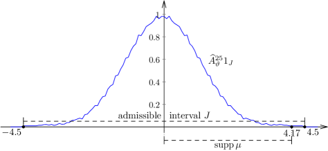
Figure 7: The function ${{\widehat{A}}_{\vartheta}}^{25}\mathds{1}_{J}\prec\mathds{1}_{J}$ for $A=\mathcal{D}_{0.75,\Lambda,\mathcal{J}}$ and $\vartheta=10^{-3}$, $\mathop{\rm supp}\nolimits\mu_{0.75}$, and an admissible interval $J$.

When it comes to the realisation of an iterative method in practice one of the common concerns is accumulation of the rounding error. The following remark explains why in the present case this is not a significant issue.

Remark 3.11.

Applying the operator $\widehat{A}_{\vartheta}$ to a given piecewise-constant function $\psi$ changes its value on one of the intervals only if the computed value $A_{\mathrm{comp}}[\psi]$ is below the actual value of $\psi$ on this interval by at least $\vartheta$, otherwise the value stays completely unchanged.

Assume that the rounding errors never exceed $\frac{1}{2}\vartheta$; this is quite reasonably the case, for instance, since we typically chose $\vartheta=10^{-8}$, while making the calculations with quadruple precision, in other words, the numbers involved have $32$ significant digits.

Then, the computed image $\widehat{A}_{\vartheta,\mathrm{comp}}[\psi]$ is lower-bounded by a true image with half the “added value”:

$$\widehat{A}_{\vartheta/2}[\psi]\preccurlyeq\widehat{A}_{\vartheta,\mathrm{comp}}[\psi].$$

By induction, it is then easy to see that after an arbitrary number $n$ of iterations one has

$$\widehat{A}_{\vartheta/2}^{n}[\psi]\preccurlyeq\widehat{A}_{\vartheta,\mathrm{comp}}^{n}[\psi].$$

Thus, if after some number $n$ of iterations the computations provide $A_{\vartheta,\mathrm{comp}}^{n}[\mathds{1}_{J}]\prec\mathds{1}_{J}$, where $A=\mathcal{D}^{(2)}_{\alpha,\mathcal{S}(\lambda)}$, one actually gets the desired $\widehat{A}_{\vartheta/2}^{n}[\mathds{1}_{J}]\prec\mathds{1}_{J}$ and hence the applicability of Corollary 3.8. In our computations, to avoid problems with the strict inequality handling, we have been asking for the inequality

$$(\widehat{\mathcal{D}^{(2)}_{\alpha,\Lambda,\mathcal{J}}})_{\vartheta,\mathrm{comp}}^{n}[\mathds{1}_{J}]\prec 0.995\cdot\mathds{1}_{J}.$$

Next, we should describe what we would do if an attempt to obtain a lower bound by a given $\alpha$ was unsuccessful.

Remark 3.12.

It is possible that after a large number of iterations $n$, there exists an interval $\mathcal{J}_{k}$ of the partition $\mathcal{J}$ where we have the equality:

$$[{{\widehat{A}}_{\vartheta}}^{n}\mathds{1}_{J}]|_{\mathcal{J}_{k}}=1.$$

Then we cannot reach a definitive conclusion, as there are three possibilities:

1. the number of iterations $n$ is not large enough,

2. the intervals of the partition $\mathcal{J}$ are too long, or the interval $\Lambda$ is too long,

3. the number $\alpha$ is not a lower bound, i.e. there exists $\lambda\in\Lambda$ such that $D_{2}(\mu_{\lambda})\leq\alpha$.

In this case we could try to increase the number of iterations, to choose a finer partition, or to drop the conjectured value $\alpha$ to $\alpha^{\prime}<\alpha$ and to consider the operator $A:=\mathcal{D}_{\alpha^{\prime},\Lambda,\mathcal{J}}$. It follows from Proposition 5.11 that provided our guess on the lower bound was correct, we will be able to justify it using this approach, subject to computer resources.

Our method can be used not only to verify a suggested lower bound, but also to find a lower bound for the correlation dimension or to improve an existing lower bound.

3.3.2 Computing a lower bound

Assume that we would like to improve an existing lower bound $d_{1}<D_{2}(\mu_{\lambda})$ using no more than $N$ iterations of the operator and piecewise constant functions with no more than $K$ intervals. Additionally assume that there is an upper bound $D_{2}(\mu_{\lambda})<d_{2}$.

Then we can fix $\varepsilon>0$, a uniform partition $\mathcal{J}$, an operator $A:=\mathcal{D}_{\alpha,\Lambda,\mathcal{J}}$ and to search for an $\alpha$ satisfying the following conditions

1. there exists $k<N$: ${{\widehat{A}}_{\vartheta}}^{k}\mathds{1}_{J}\prec\mathds{1}_{J}$

2. for all $k\leq N$: ${{\widehat{A}}_{\vartheta}}^{k}\mathds{1}_{J}\not\prec\mathds{1}_{J}$

One approach to find $\alpha$ would be to apply the well known bisection method to the interval $(d_{1},d_{2})$. However, to obtain good estimates, one has to allow for a large number of iterations before dropping the conjectured lower bound and this is very time-consuming. In other words, negative answer is expensive as we have to examine all possibilities described in Remark 3.12.

It is therefore more efficient to use a partition of the interval $(d_{1},d_{2})$ into $M\!:=\![\sqrt{(d_{2}\!-\!d_{1})\varepsilon^{-1}}]$ intervals of equal length and to test the values $\alpha_{k}=d_{1}+k\cdot\frac{1}{M}$, $k=1,\ldots,M$ using the method explained in the previous subsection 3.3.1. We then want to find a $0\leq k\leq M$ such that for $A_{k}:=\mathcal{D}_{\alpha_{k},\Lambda,\mathcal{J}}$ there exists $n<N$ with the property

$${\widehat{A}_{k,\vartheta}}^{n}\mathds{1}_{J}\prec\mathds{1}_{J}\qquad\mbox{ and }\qquad{\widehat{A}_{k+1,\vartheta}}^{N}\mathds{1}_{J}\not\prec\mathds{1}_{J}.$$

Then we repeat the procedure again, dividing the interval $\left(\alpha_{k},\alpha_{k+1}\right)$ into $M$ intervals of length $\varepsilon$. This way would need to apply all $N$ iterations only twice (to confirm the second condition (ii)) to find the desired value $\alpha$.

Finally, we note that in order to compute a good lower bound on a large interval of parameter values, we consider a cover of this interval by a large number of small overlapping intervals and compute a lower bound on each of them.

Remark 3.13.

We would like to emphasize that the value $\alpha+\varepsilon$ is not an upper bound for correlation dimension, as it depends on the number $K$ of iterations allowed and the number of intervals for the space of piecewise constant functions, and might increase (together with $\alpha$) when we increase those values.

Definition 3.14.

We call $\varepsilon$ the refinement parameter.

In Subsection 3.3.3 we give details of the application of our method to computing lower bound for correlation dimension of Bernoulli convolutions.

We conclude this subsection by presenting the following alternate approach to the use of the diffusion operator, that was suggested to us by an anonymous referee. This suggestion is particularly helpful, and we are glad to be able to present it here:

Remark 3.15.

For a given sufficiently small interval $\Lambda$ of values of $\lambda$ one can:

• Take the initial function $\psi_{0}=\mathds{1}_{J}$, sufficiently small $\vartheta$, initial lower bound $\alpha_{0}$ and a threshold $t\in(0,1)$;

• Apply the operator ${{\widehat{A}}_{\vartheta}}$, where $A=D_{\alpha_{0},\Lambda,\mathcal{J}}$, until the maximum descends below the chosen threshold. Let $k$ be the smallest number such that

  $$\psi:={{\widehat{A}}_{\vartheta}}^{k}\mathds{1}_{J}\prec t\cdot\mathds{1}_{J}.$$ (17)

  In particular, as $t<1$, this implies that ${{\widehat{A}}_{\vartheta}}[\psi]\preccurlyeq\psi$;

• Then, one gets a lower bound $\alpha$ for the correlation dimension, choosing its value to be the maximal for which $D_{\alpha,\Lambda,\mathcal{J}}[\psi]\preccurlyeq\psi$, by setting

  $$\alpha:=\alpha_{0}+\log_{\lambda_{\min}}\max_{J}\frac{D_{\alpha_{0},\Lambda,\mathcal{J}}[\psi]}{\psi}=\log_{\lambda_{\min}}\max_{J}\frac{D_{0,\Lambda,\mathcal{J}}[\psi]}{\psi},$$ (18)

  where $\lambda_{\min}=\min\Lambda$. Observe that since one can actually use any function $\psi$ in order to look for the lower bound $\alpha$ (applying then Theorem 3.2), rounding errors during the iterations are not much of an issue. Indeed, there is only one iteration and one division applied in (18), with the denominator bounded from below by $\vartheta$ due the construction of $\psi$, and compared to the precision of calculations $\vartheta$ is not a small number at all.

This method really works quite well. For instance, taking $\vartheta=10^{-7}$ and $\alpha_{0}=0.82$ (lower bound by Hare and Sidorov), taking $\Lambda$ to be $0.5\cdot 10^{-5}$-neighborhood of some $\lambda$ and separating the interval $J=[-r,r]$ into $4\cdot 10^{4}$ intervals, where $r=\frac{1.1}{1-\lambda_{\max}}$, $\lambda_{\max}=\max\Lambda$, and choosing the threshold $t=\frac{1}{20}$ (that is quite small so that $k$ in (17) is quite large), one gets the estimates

• $\alpha=0.9923757365$ for the Fibonacci value $\lambda=0.6180339887$ (compare with the lower bound $0.992395833333$ in Table 5);

• $\alpha=0.9642020738$ for the tribonacci value $\lambda=0.54368901$ (compare with the lower bound $0.964214555664$ in Table 5);

• $\alpha=0.999641567$ for one of the Salem numbers $\lambda=0.71363917$ (compare with the lower bound $0.999687500$ in the table in Section A.1).

3.3.3 Proof of Theorem 1.4

Recall that $\dim_{H}\mu_{\lambda}\geq\dim_{H}\mu_{\lambda^{2}}$ and therefore it is sufficient to compute a lower bound for $\lambda\in[0.5,0.8]$.

To obtain a uniform lower bound on the correlation dimension $D_{2}(\mu_{\lambda})$, for Bernoulli convolution measures $\mu_{\lambda}$ on the entire interval of parameter values $[0.5,0.8]$ we proceed in two steps. First, we consider a cover of the interval $[0.5,0.8]$ by $100$ overlapping intervals of the same size. We then apply the method explained in §3.3.2 with $N=7\cdot 10^{6}$ partition intervals for the test function, and set the maximum for the number of iterations of the diffusion operator to $K=150$. We choose a lower bound $d_{1}=0.82$, an upper bound $d_{2}=1$ and set the refinement parameter to $\varepsilon=0.01$. The computation takes about 10 minutes for each interval and can be done in parallel; the result is presented in Table 3.

$\Lambda$		$\alpha$	$\Lambda$		$\alpha$
$[0.500,0.515]$		$0.96612$	$[0.566,0.569]$		$0.96612$
$[0.515,0.518]$		$0.95402$	$[0.569,0.614]$		$0.97822$
$[0.518,0.542]$		$0.96370$	$[0.614,0.617]$		$0.96612$
$[0.542,0.545]$		$0.95402$	$[0.617,0.743]$		$0.97580$
$[0.545,0.554]$		$0.96612$	$[0.743,0.800]$		$0.96612$
$[0.554,0.566]$		$0.97580$

Table 3: Uniform lower bounds for the correlation dimension of Bernoulli convolution measures, after the first step.

Afterwards, we use the bounds we computed as an initial guess for the corresponding parameters $\lambda$ and improve them by applying the same method again. This time, based on the first estimates, we take uniform covers of $[0.499,0.575]$ and $[0.572,0.8]$ by $5000$ intervals each. We then use $N=10^{7}$ intervals for the space of piecewise-constant functions; set the maximum $K=1000$ for the number of iterations for the diffusion operator; and choose $\varepsilon=10^{-4}$ as the refinement parameter. This second computation takes about two weeks with 32 threads running in parallel.

The result is presented in Figure 9. In support of the conjecture that dimension drops occur at Pisot parameter values, we identify minimal polynomials of algebraic numbers which seem to correspond to the bigger drops and verified that they are Pisot values, i.e. all their Galois conjugates lie inside the unit circle.

Remark 3.16.

It follows from the overlaps conjecture by Simon [32] which was proved by Hochman [17] for algebraic parameter values, that the dimension drop occurs only for the roots of polynomials with coefficients $\{-1,0,1\}$. We see that some of the polynomials indicated in the plot have $\pm 2$ among their coefficients. This doesn’t contradict the result of Hochman, because the polynomials we give are the minimal polynomials. Each of the polynomials with coefficients $\pm 2$ becomes a polynomial with coefficients $\{-1,0,1\}$ after multiplying by an appropriate factor. For instance, $x^{5}-x^{3}-2x^{2}-2x-1$ after multplying by $(x-1)$ becomes $x^{6}-x^{5}-x^{4}-x^{3}+x+1$.

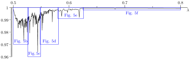
(a) Plot of lower bounds for correlation dimension of Bernoulli convolution measures for $0.5\leq\lambda\leq 0.8$ with more detailed plots in 8(b), 8(c), 9(a), 9(b), 9(c) below.

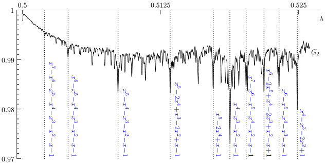
(b) $0.499<\lambda<0.526$

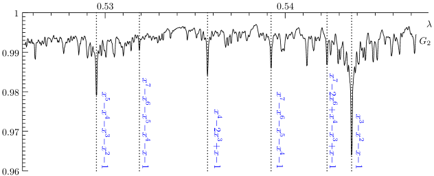
(c) $0.523<\lambda<0.548$

Figure 8: The plot of the piecewise constant function $G_{2}(\lambda)$, which gives lower bounds on correlation dimension of Bernoulli convolution $D_{2}(\mu_{\lambda})$.

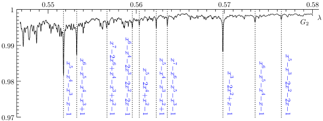
(a) $0.548<\lambda<0.58$

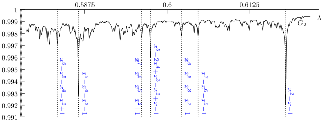
(b) $0.58<\lambda<0.625$

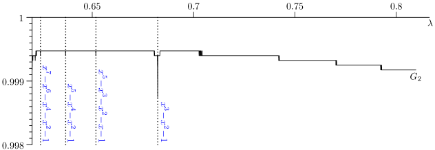
(c) $0.625<\lambda<0.81$

Figure 9: (Continued). The plot of the piecewise constant function $G_{2}(\lambda)$, which gives lower bounds on correlation dimension of Bernoulli convolution $D_{2}(\mu_{\lambda})$. The polynomials indicated are the minimal polynomials of the corresponding values $\lambda$, which are Pisot.

Based on the graph of the lower bound function $G_{2}(\lambda)$ shown in Figure 9 we conjecture that for reciprocals of Fibonacci $\lambda=2/(1+\sqrt{5})$ and “tribonacci” ($\lambda=\beta^{-1}$, where $\beta$ is the largest root of $x^{3}-x^{2}-x-1$) parameter values there exists a sequence $\lambda_{n}^{\prime}$ of Pisot numbers such that $\lambda_{n}^{\prime}\to\lambda$ as $n\to\infty$ such that the dimensions $D_{2}(\mu_{\lambda^{\prime}_{n}})<1-\varepsilon$ for some $\varepsilon>0$ and moreover the limit $\lim_{n\to\infty}D_{2}(\mu_{\lambda^{\prime}_{n}})<1$.

3.3.4 Proof of Theorem 1.13

Contrary to the case of Bernoulli convolutions, there were no apriori estimates on dimension drop known.

First, we consider a cover of the interval of parameter values $(0.249,0.334)$ by $100$ overlapping intervals $\Lambda_{k}$, $k=1,\ldots,100$. We set the limit $K=200$ for the number of iterations and $N=10^{5}$ for the number of intervals for piecewise constant functions. We then choose $\varepsilon=0.01$ as the refinement parameter and $d_{1}=0.5$, $d_{2}=-\frac{\log 3}{\log\inf\Lambda_{k}}$ as lower and upper bounds, respectively. Applying the algorithm described in Section 3.3.2 we obtain rough estimates. The result is presented in Table 4. Afterwards, we improve this estimate. We choose the refinement parameter $\varepsilon=10^{-4}$, set $N=10^{7}$ to be the number of intervals for the step function, $K=1000$ for the maximal number of iterations and choose the lower bound which was already computed.

The lower bounds for $\lambda\in(0.333,0.401)$ we compute applying the same steps with $d_{0}=0$ and $d_{1}=1$.

$\Lambda$	$\alpha$	$\Lambda$	$\alpha$
$[0.25000,0.26501]$	$0.77082$	$[0.32839,0.33173]$	$0.85657$
$[0.26501,0.26918]$	$0.79581$	$[0.33173,0.33434]$	$0.79659$
$[0.26918,0.28169]$	$0.80051$	$[0.33434,0.33702]$	$0.87375$
$[0.28169,0.28669]$	$0.83549$	$[0.33702,0.34372]$	$0.89479$
$[0.28669,0.29086]$	$0.85245$	$[0.34372,0.34908]$	$0.91583$
$[0.29086,0.30587]$	$0.83663$	$[0.34908,0.35712]$	$0.94388$
$[0.30587,0.30838]$	$0.87025$	$[0.35712,0.36717]$	$0.91583$
$[0.30838,0.31338]$	$0.86111$	$[0.36717,0.37722]$	$0.95440$
$[0.31338,0.32089]$	$0.88076$	$[0.37722,0.38526]$	$0.95791$
$[0.32089,0.32839]$	$0.86694$	$[0.38526,0.40000]$	$0.98246$

Table 4: Uniform lower bounds for the correlation dimension of the stationary measure in the $\{0,1,3\}$-problem, after the first step.

The result is presented in Figure 11. We managed to identify minimal polynomials of algebraic numbers which seem to correspond to some of the biggest dimension drops and verified that the corresponding parameter values are reciprocals of hyperbolic numbers. In the case of the $\{0,1,3\}$-system, the overlaps conjecture implies that the dimension drop for algebraic parameter values takes place only for the roots of polynomials with coefficients $\{0,\pm 1,\pm 2,\pm 3\}$, and the polynomials we have identified satisfy this property.

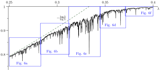
(a) Plot of lower bounds for correlation dimension of Bernoulli convolution measures for $0.249\leq\lambda\leq 0.401$ with more detailed plots in 10(b), 10(c), 11(a), 11(b), 11(c) below.

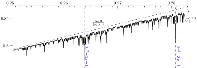
(b) $0.25<\lambda<0.283$

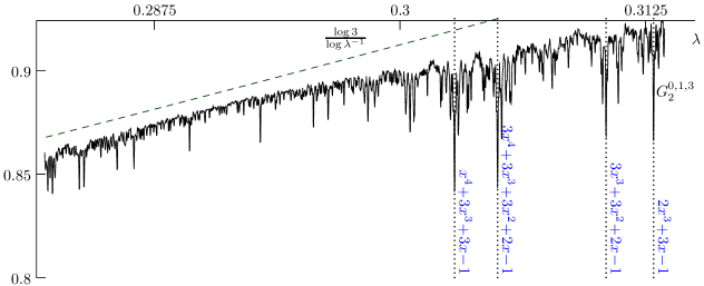
(c) $0.2825<\lambda<0.3128$

Figure 10: The plot of the piecewise constant function $G^{0,1,3}_{2}(\lambda)$, which gives lower bounds on Hausdorff dimension $D_{2}(\mu^{0,1,3}_{\lambda})$ of the stationary measure for the $\{0,1,3\}$-system. The polynomials indicated are the minimal polynomials of the corresponding values $\lambda$, which are hyperbolic.

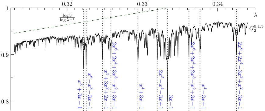
(a) $0.312<\lambda<0.345$

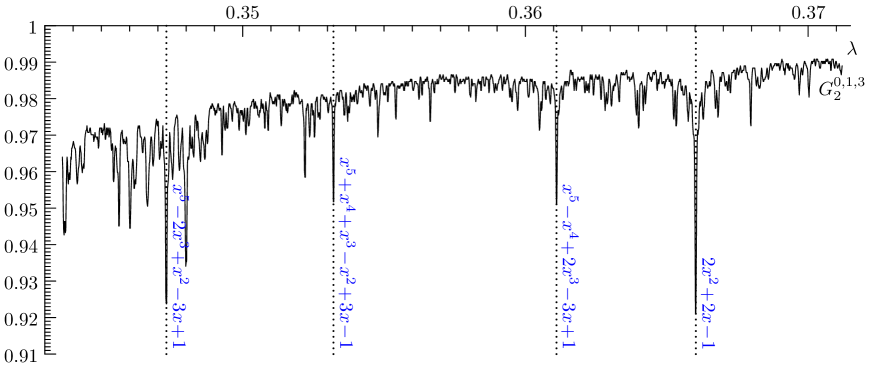
(b) $0.3445<\lambda<0.3715$

(c) $0.3710<\lambda<0.4$

Figure 11: The plot of the piecewise constant function $G^{0,1,3}_{2}(\lambda)$, which gives lower bounds on Hausdorff dimension $D_{2}(\mu^{0,1,3}_{\lambda})$ of the stationary measure for the $\{0,1,3\}$-system.

3.4 Selected algebraic parameter values

So far we have applied our method to compute uniform lower bounds on dimension of the stationary measures. As we highlighted already in the end of §3.2, in order to get a lower bound on $D_{2}(\mu_{\lambda})$ for an algebraic $\lambda$, we need to consider a small interval containing the value. In this section, we compute a lower bound on correlation, and hence Hausdorff, dimensions of $\mu_{\lambda}$, for selected algebraic values and compare our results with the existing data. For some specific values these results are not as accurate as existing estimates. For other parameter values, e.g. Salem numbers, we give a new improved lower bound.

We begin by recalling some known results. In [11] Garsia introduced a notion of entropy of an algebraic number $\lambda$ (also see [15] for an alternative definition)

$$h(\lambda)=\lim_{N\to+\infty}-\frac{1}{2^{n}}\sum_{i_{1},\cdots,i_{N}\in\{0,1\}}\log\left(\frac{1}{2^{n}}\hbox{\rm Card}\left\{j_{1},\cdots,j_{N}\in\{0,1\}\hbox{ : }\sum_{k=1}^{n}(i_{k}-j_{k})\lambda^{k}=0\right\}\right).$$

Garsia entropy was first used to estimate Hausdorff dimension of Bernoulli convolution corresponding to the Golden mean $\lambda=\frac{2}{1+\sqrt{5}}$. The method has been subsequently extended in [12] to the roots of the polynomials

$$P_{n}(x)=x^{n}-x^{n-1}-\ldots-x-1.$$

In Table 5 we give a comparison of the lower bounds we have computed using the diffusion operator and the results of Grabner at al. [12]. This illustrates that our bounds are quite close to the known values.

$n$	$\dim_{H}(\mu_{\lambda})$	$\alpha$	$n$	$\dim_{H}(\mu_{\lambda})$	$\alpha$
$2$	$0.995713126685555$	$0.992395833333$	$6$	$0.996032591584967$	$0.990673828125$
$3$	$0.980409319534731$	$0.964214555664$	$7$	$0.997937445507094$	$0.994959490741$
$4$	$0.986926474333800$	$0.973324567994$	$8$	$0.998944915449832$	$0.997343750000$
$5$	$0.992585300274171$	$0.983559570313$	$9$	$0.999465368055570$	$0.998640046296$

Table 5: Comparison of the lower bound for the correlation dimension $\alpha<D_{2}(\mu_{\lambda})$ computed using the diffusion operator and the Hausdorff dimension computed in [12, §4] for mutlinacci parameter values.

The connection between $h(\lambda)$ and $\dim_{H}(\mu_{\lambda})$ comes by a result of Hochman [17]:

$$\dim_{H}(\mu_{\lambda})=\min\left\{-\frac{h(\lambda)}{\log\lambda},1\right\}.$$ (19)

However, despite (19) being exact, the value $h(\lambda)$ for algebraic numbers is often quite difficult to estimate for all but a small number of examples, see [1] (also [22]) which gave algorithms to compute the entropy based on Lyapunov exponents of random matrix products. For several explicit (non-Pisot) examples they showed that $\frac{h(\lambda)}{\log(\lambda^{-1})}>1$; together with (19) this implies $\dim_{H}(\mu_{\lambda})=1$.

On the other hand, Breuillard and Varjú [3] gave an estimate on $h(\lambda)$ in terms of the Mahler measure $M_{\lambda}$:

$$c\cdot\min\left\{1,\log M_{\lambda}\right\}\leq h(\lambda)\leq\min\left\{1,\log M_{\lambda}\right\}.$$ (20)

Non-rigorous numerical calculations suggest that one can take $c=0.44$. The upper bound in (20) is often strict. In particular, it is known that $h(\lambda)<M_{\lambda}$, provided $\lambda$ has no Galois conjugates on the unit circle [3].

The dimension of the Bernoulli convolution measure for certain hyperbolic parameter values $\lambda$ can be computed explicitly, too. In a recent work [15] Hare et al. considered hyperbolic algebraic numbers of degree $5$. For a number of them they showed that the stationary measure has full Hausdorff dimension [15, Tables 5.1, 5.2]. We present our lower bound for the correlation dimension for comparison in Table 6, which shows that our lower bounds are accurate to $3$ decimal places.

$\lambda$	$\alpha$	$\beta=\lambda^{-1}$	polynomial
$0.862442360254$	$0.999609375000$	$1.159497777573$	$x^{5}+x^{4}-x^{3}-x^{2}-1$
$0.827590407756$	$0.999687500000$	$1.208327199818$	$x^{5}-x^{4}+x^{3}-x-1$
$0.874449227129$	$0.999609375000$	$1.143576972768$	$x^{5}+x^{3}-x^{2}-x-1$
$0.710434255787$	$0.999843750000$	$1.407589783086$	$x^{5}-x^{4}+x^{3}-x^{2}-x-1$
$0.779544663821$	$0.999765625000$	$1.282800135015$	$x^{5}-x^{3}-x^{2}+x-1$
$0.791906429308$	$0.999765625000$	$1.262775452996$	$x^{5}-x^{4}+x^{2}-x-1$
$0.786151377757$	$0.999765625000$	$1.272019649514$	$x^{4}-x^{2}-1$
$0.699737022113$	$0.999843750000$	$1.429108319838$	$x^{5}-x^{3}-x^{2}-1$
$0.779544663821$	$0.999765625000$	$1.282800135015$	$x^{5}-x^{3}-x^{2}+x-1$
$0.800094994405$	$0.999765625000$	$1.249851588864$	$x^{5}-x^{4}+x^{3}-x^{2}-1$
$0.876611867657$	$0.999609375000$	$1.140755717433$	$x^{5}+x^{4}-x^{3}-x-1$
$0.655195524260$	$0.999843750000$	$1.526261952307$	$x^{5}-x^{4}-x^{2}-x+1$
$0.848374895732$	$0.999687500000$	$1.178724176105$	$x^{4}+x^{3}-x^{2}-x-1$
$0.819172513396$	$0.999687500000$	$1.220744084605$	$x^{4}-x-1$
$0.774804113215$	$0.999765625000$	$1.290648801346$	$x^{4}-x^{3}+x^{2}-x-1$
$0.730440478359$	$0.999843750000$	$1.369036943635$	$x^{5}-x^{3}-x^{2}-x+1$
$0.833363173425$	$0.999687500000$	$1.199957031806$	$x^{5}-x^{3}+x^{2}-x-1$

Table 6: Lower bound $\alpha<D_{2}(\mu)$ for the correlation dimension for selected algebraic numbers for which it is known [15] that $\dim_{H}(\mu_{\lambda})=1$, computed using $5\cdot 10^{6}$ partition intervals and $500$ iterations of the diffusion operator with the refinement parameter $\varepsilon=10^{-4}$. The value of the root $\beta$ is given to simplify the comparison with [15].

On the other hand, there are a number of algebraic parameter values to which the method presented in [15] doesn’t apply, they are listed in [15, Table 5.3]. For these values we give a new lower bound in Table 7.

$\lambda$	$\alpha$	$\beta=\lambda^{-1}$	polynomial
$0.593423522613$	$0.998714285714$	$1.685137110165$	$z^{5}-z^{4}-z^{2}-z-1$
$0.595089298038$	$0.999000000000$	$1.680420070225$	$z^{5}-z^{4}-z^{3}-z+1$
$0.557910446633$	$0.997857142857$	$1.792402357824$	$z^{5}-z^{4}-z^{3}-z^{2}+z-1$
$0.712452611946$	$0.999800000000$	$1.403602124874$	$z^{5}-z^{4}-z^{2}+z-1$
$0.645200388386$	$0.999800000000$	$1.549906072594$	$z^{5}-z^{4}-z^{3}+z-1$
$0.667960707496$	$0.999800000000$	$1.497094048762$	$z^{5}-z^{4}-z-1$
$0.808730600479$	$0.999600000000$	$1.236505703391$	$z^{5}-z^{3}-1$
$0.837619774827$	$0.999722222222$	$1.193859111321$	$z^{5}-z^{2}-1$
$0.856674883855$	$0.999652777778$	$1.167303978261$	$z^{5}-z-1$
$0.889891245776$	$0.999513888889$	$1.123732821001$	$z^{5}+z^{4}-z^{2}-z-1$

Table 7: Lower bound $\alpha<D_{2}(\mu)$ for the correlation dimension for selected algebraic numbers for which there are no previous lower bounds, computed using $5\cdot 10^{6}$ partition intervals and $500$ iterations of the diffusion operator and the refinement parameter $\varepsilon=10^{-4}$. The value of the root $\beta$ is given to simplify the comparison with [15].

3.4.1 Estimates for Salem numbers: Proof of Theorem 1.7

In a recent work, Breuillard and Varjú state an open problem [3, Problem 3], asking whether it is true that $h(\lambda)=M_{\lambda}$ for all Salem parameter values $\lambda\in\left(\frac{1}{2},1\right)$. This equality would imply that $\dim_{H}(\mu_{\lambda})=1$ for Salem parameter values.

We apply the method described in §3.3.2 to $99$ Salem numbers of degree no more than $10$ and to $47$ small Salem numbers. Our computational set-up had the following choices. First, we compute each Salem number $s_{k}$ with an accuracy of $10^{-32}$ and consider a neighbourhood of radius $\delta=10^{-8}$, i.e. $\Lambda_{k}=B_{\delta}(s_{k})$. Then, based on the existing results, we choose $d_{1}=0.98$ and $d_{2}=1$, as conjectured lower and upper bounds. The number of intervals for piecewise constant functions is $N=6\cdot 10^{5}$, and the allowed number of iterations for the diffusion operator is $K=300$. We also set the refinement parameter $\varepsilon=10^{-4}$. The detailed result is presented in Appendix §A.1 and §A.2.

4 Asymptotic bounds: proof of Theorem 1.8

We have provided a uniform lower bound on the correlation dimension $D_{2}(\mu_{\lambda})$ of Bernoulli convolution measures $\mu_{\lambda}$. Now we will give an asymptotic lower bound for $D_{2}(\mu_{\lambda})$ in a neighbourhood of $1$ using the diffusion operator approach.

Proof of Theorem 1.8. Given a small $\varepsilon>0$ let us set $\lambda=1-\varepsilon$. Then the symmetric diffusion operator (5) takes the form

$$[\mathcal{D}^{(2)}_{\alpha,\mathcal{S}}\psi](x)=(1-\varepsilon)^{-\alpha}\frac{1}{4}\left(\psi\left(\frac{x+1}{1-\varepsilon}\right)+2\psi\left(\frac{x}{1-\varepsilon}\right)+\psi\left(\frac{x-1}{1-\varepsilon}\right)\right)$$

In order to prove the result, it is sufficient to find a function $f_{\varepsilon}$ such that for any $c>\frac{3}{2}$ and for any $\alpha<1-c\varepsilon$ we have that

$$\mathcal{D}^{(2)}_{\alpha,\mathcal{S}}f_{\varepsilon}\prec f_{\varepsilon}.$$ (21)

We will specify the function $f_{\varepsilon}$ explicitly. Let us introduce a shorthand notation $\delta:=2\varepsilon-\varepsilon^{2}>0$ and define

$$f_{\varepsilon}(x):=\exp(-\delta(1-\varepsilon)^{2}x^{2})=\exp(-\delta x^{2})\cdot\exp(\delta^{2}x^{2})$$ (22)

It is not difficult to see that $f_{\varepsilon}$ satisfies (21). Indeed, note that $\frac{1+\exp(-\delta)}{2}\leq(1-\varepsilon)^{1-c\varepsilon}$ for any $\varepsilon$ sufficiently small and any $c>\frac{3}{2}$. Therefore to establish (21) it is sufficient to show that

$$\frac{1}{4}\left(f_{\varepsilon}\left(\frac{x+1}{1-\varepsilon}\right)+f_{\varepsilon}\left(\frac{x-1}{1-\varepsilon}\right)+2f_{\varepsilon}\left(\frac{x}{1-\varepsilon}\right)\right)\leq\frac{1+\exp(-\delta)}{2}f_{\varepsilon}(x).$$ (23)

To prove (23) we first note that

$$f_{\varepsilon}\left(\frac{x+1}{1-\varepsilon}\right)+f_{\varepsilon}\left(\frac{x-1}{1-\varepsilon}\right) =\exp(-\delta(x+1)^{2})+\exp(-\delta(x-1)^{2})$$

$$=\exp(-\delta)\cdot\exp(-\delta x^{2})\left(\exp(-2\delta x)+\exp(2\delta x)\right)$$

$$=2\exp(-\delta)\cdot\exp(-\delta x^{2})\cdot\cosh(2\delta x).$$

Moreover, since $f_{\varepsilon}\left(\frac{x}{1-\varepsilon}\right)=\exp(-\delta x^{2})$ we conclude for the left hand side of (23) that

$$\frac{1}{4}\left(f_{\varepsilon}\left(\frac{x+1}{1-\varepsilon}\right)+f_{\varepsilon}\left(\frac{x-1}{1-\varepsilon}\right)+2f_{\varepsilon}\left(\frac{x}{1-\varepsilon}\right)\right)=\frac{1}{2}\exp(-\delta x^{2})\cdot\left(1+\cosh(2\delta x)\exp(-\delta)\right).$$ (24)

Combining (22) and (24) we see that (23) is equivalent to

$$1+\exp(-\delta)\cosh(2\delta x)\leq(1+\exp(-\delta))\exp\left(\delta^{2}x^{2}\right),$$

which in turn, is equivalent to

$$\frac{1}{1+\exp(-\delta)}+\frac{\exp(-\delta)}{1+\exp(-\delta)}\cosh(2\delta x)\leq\exp\left(\delta^{2}x^{2}\right),$$ (25)

To establish (25) it is sufficient to show that

$$\frac{1}{2}+\frac{1}{2}\cosh(2\delta x)\leq\exp\left(\delta^{2}x^{2}\right).$$

This last inequality can be established by comparision of the Taylor series coefficients term by term. More precisely, the coefficient in front of the term $(\delta x)^{2k}$ of the function $\cosh(2\delta x)$ is $\frac{2^{2k}}{(2k)!}$ and the same coefficient of the function $\exp\left(\delta^{2}x^{2}\right)$ is equal to $\frac{1}{k!}$. $\blacksquare$

5 Diffusion operator $\mathcal{D}^{(2)}_{\alpha,\lambda}$ and correlation dimension

We would like to start by explaining the idea behind the diffusion operator and its connection with the correlation dimension which lead us to it.

Let us recall the energy integral (10)

$$I(\mu,\alpha)=\int_{\mathbb{R}}\int_{\mathbb{R}}|x-y|^{-\alpha}\mu(dx)\mu(dy)$$

and the definition of the correlation dimension (11): $D_{2}(\mu)=\sup\{\alpha\colon I(\mu,\alpha)\mbox{ is finite }\}$. In other words, $I(\mu,\alpha)$ is finite for any $\alpha<D_{2}(\mu)$.

Let $\mathcal{S}(\lambda,\bar{c},\bar{p})$ be an iterated function scheme of $n$ similarities $f_{j}=\lambda x-c_{j}$, $j=1,\ldots,n$ and let $\mu_{\lambda}$ be its stationary measure. Then $\mu_{\lambda}$ is the fixed point of the operator on Borel probability measures

$$T_{\mathcal{S}}\colon\mu\mapsto\sum_{j=1}^{n}p_{j}{f_{j}}_{*}\mu$$

We now would like to study the induced action of $T_{\mathcal{S}}$ on $I(\mu,\alpha)$. To this end, we want to incorporate $I(\mu,\alpha)$ into a family. More precisely, we consider a family of functions given by

$$\psi_{\alpha,\mu}:\mathbb{R}\to\mathbb{R}^{+}\cup\{+\infty\}\qquad\psi_{\alpha,\mu}(r):=\int_{\mathbb{R}}\int_{\mathbb{R}}|(x-y)-r|^{-\alpha}\,\mu(dx)\,\mu(dy).$$ (26)

Notation 5.1.

We denote by $-\mu$ the push-forward of the measure $\mu$ under $x\mapsto-x$.

In the sequel, we will need the following technical lemma which helps us to decide whether or not $\psi_{\alpha,\mu}(r)$ is finite.

Lemma 5.2.

Let $\mu$ be a probability measure. Assume that $I(\mu,\alpha)=\psi_{\alpha,\mu}(0)$ is finite. Then $\psi_{\alpha,\mu}(r)$ is finite for any $r\in\mathbb{R}$ and, moreover, we have that $\psi_{\alpha,\mu}(r)<\psi_{\alpha,\mu}(0)$. In particular, $\psi_{\alpha,\mu}$ is a continuous function.

Proof . Let us denote $\nu\colon=\mu*(-\mu)$. It is easy to see that its Fourier transform is a nonnegative function:

$$\hat{\nu}(t)=\int_{\mathbb{R}}e^{-itz}\nu(dz)=\int_{\mathbb{R}}\int_{\mathbb{R}}e^{-it(x-y)}\mu(dx)\mu(dy)=\hat{\mu}(t)\overline{\hat{\mu}(t)}=|\mu(t)|^{2}\geq 0.$$

We may write

$$\psi_{\alpha,\mu}(r)=\int_{\mathbb{R}^{2}}|x-y-r|^{-\alpha}\mu(dx)\mu(dy)=\int_{\mathbb{R}}|z-r|^{-\alpha}\nu(dz).$$

Then the desired inequality $\psi_{\alpha,\mu}(r)<\psi_{\alpha,\mu}(0)$ for all $r\in\mathbb{R}$ is equivalent to

$$\int_{\mathbb{R}}|z-r|^{-\alpha}\nu(dz)\leq\int_{\mathbb{R}}|z|^{-\alpha}\nu(dz).$$

Let us consider the function $f_{\alpha}(s)\buildrel\rm def\over{=}|s|^{-\alpha}$. Its Fourier transform is known to be

$$\hat{f}_{\alpha}(t)=\frac{\pi^{\alpha-1/2}\Gamma\left((1-\alpha)/2\right)}{\Gamma(\alpha/2)}|t|^{\alpha-1}=C_{\alpha}|t|^{\alpha-1}\geq 0,\quad 0<\alpha<1.$$ (27)

where $C_{\alpha}=\frac{\pi^{\alpha-1/2}\Gamma\left((1-\alpha)/2\right)}{\Gamma(\alpha/2)}$. Therefore $\widehat{f_{\alpha}*\nu_{\lambda}}=\hat{f}_{\alpha}\cdot\hat{\nu}_{\lambda}$ is real and non-negative. Using the inverse Fourier transform formula we obtain an upper bound.

$$\psi_{\alpha,\mu}(r)=\int_{\mathbb{R}}|z-r|^{-\alpha}\nu(dz)=(f_{\alpha}*\nu)(r)=\frac{1}{2\pi}\int_{\mathbb{R}}e^{-itr}\hat{f}_{\alpha}(t)\cdot\hat{\nu}(t)dt\\ \leq\frac{1}{2\pi}\int_{\mathbb{R}}\hat{f}_{\alpha}(t)\cdot\hat{\nu}(t)dt=\psi_{\alpha,\mu}(0)<\infty.$$

The function $\psi_{\alpha,\lambda}$ is continuous since it is an inverse Fourier transform of an $L_{1}$ function.

$\blacksquare$

Remark 5.3.

Let $m=\inf\{x\mid\mathop{\rm supp}\nolimits\mu*(-\mu)\subseteq[-x,x]\}$ and let $J=[-a,a]\supsetneq[-m,m]$. Then $\psi_{\alpha,\mu}$ has a bounded continuous extension to $\mathbb{R}\setminus J$ with an upper bound

$$\psi_{\alpha,\mu}(r)\leq(m-a)^{-\alpha}\quad\mbox{ for all }r,\,|r|>a.$$

Therefore, the behaviour of $\psi_{\alpha,\mu}$ on $\mathop{\rm supp}\nolimits\mu*(-\mu)$ is the most important to us. The next Proposition ties together the symmetric diffusion operator $\mathcal{D}^{(2)}_{\alpha,\mathcal{S}}$, a family of functions $\psi_{\alpha,\mu}$, and the action on measures $T_{\mathcal{S}}$.

Proposition 5.4.

Let $\mathcal{S}(\lambda,\bar{c},\bar{p})$ be an iterated function scheme of $n$ similaritites. Let $\mu$ be a probability measure such that $\mathop{\rm supp}\nolimits\mu\subset J$ for a closed interval $J$. Assume that for some $\alpha>0$ the function $\psi_{\alpha,\mu}$ is bounded. Then

$$\psi_{\alpha,T_{\mathcal{S}}\mu}=\mathcal{D}^{(2)}_{\alpha,\mathcal{S}}\psi_{\alpha,\mu}.$$

Proof . For convenience, recall the definition of the symmetric diffusion operator (5):

$$[\mathcal{D}^{(2)}_{\alpha,\mathcal{S}}\psi](x):=\lambda^{-\alpha}\cdot\sum_{i,j=1}^{k}p_{i}p_{j}\cdot\psi\left(\frac{x+c_{i}-c_{j}}{\lambda}\right).$$

By straightforward computation,

$$\psi_{\alpha,T_{\mathcal{S}}\mu}(r) =\int\int|y-(x-r)|^{-\alpha}T_{\mathcal{S}}\mu(dx)T_{\mathcal{S}}\mu(dy)$$

$$=\int\int|y-(x-r)|^{-\alpha}\left(\sum p_{j}{f_{j}}_{*}\mu\right)(dx)\left(\sum p_{k}{f_{k}}_{*}\mu\right)(dy)$$

$$=\sum_{j,k}p_{j}p_{k}\int\int|f_{j}(x)-(f_{k}(y)-r)|^{-\alpha}\mu(dx)\mu(dy)$$

$$=\sum_{j,k}p_{j}p_{k}\int\int|\lambda x-c_{j}-\lambda y+c_{k}+r|^{-\alpha}\mu(dx)\mu(dy)$$

$$=\lambda^{-\alpha}\sum_{j,k}p_{j}p_{k}\int\int\left|x-y+\lambda^{-1}(r-c_{j}+c_{k})\right|^{-\alpha}\mu(dx)\mu(dy)$$

$$=\lambda^{-\alpha}\sum_{j,k}p_{j}p_{k}\psi_{\alpha,\mu}\left(\lambda^{-1}(r-c_{j}+c_{k})\right)=[\mathcal{D}^{(2)}_{\alpha,\mathcal{S}}\psi](r).$$

$\blacksquare$

Corollary 5.5.

Let $\mu$ be the unique stationary measure $\mu$ of an iterated function scheme $\mathcal{S}(\lambda,\bar{c},\bar{p})$. Assume that $I(\mu,\alpha)$ is bounded. Then $\psi(\alpha,\mu)$ is the fixed point of $\mathcal{D}^{(2)}_{\alpha,\mathcal{S}}$.

Remark 5.6.

Of course the constant function $f\equiv 1\subset L^{\infty}(\mathbb{R})$ is an eigenvector for the diffusion operator with the eigenvalue $\lambda^{-\alpha}$, but it does not satisfy the hypothesis of Theorem 1.17 and is of no use to us.

In the next section we give a proof for Theorem 1.17, which provides the grounds for the numerical estimates of the correlation dimension.

5.1 Random processes viewpoint

The random processes viewpoint will be used in the arguments for Theorems 1.17, 1.19, 1.23, and 1.25. We would like therefore to make a preparatory description of the setup.

Definition 5.7.

Let $\mathcal{S}\left(\lambda,\bar{c},\bar{p}\right)$ be an iterated function scheme. We want to consider the set of pairwise differences $\{d_{k}\mid d_{k}=c_{i}-c_{j}\}$, a probability vector $q_{k}=\sum\limits_{i,j\colon c_{i}-c_{j}=d_{k}}p_{i}p_{j}$, and to define a complementary iterated function scheme $\mathcal{S}(\lambda,\bar{d},\bar{q})$:

$$g_{k}(x)=\lambda x-d_{k}.$$

If $\mu$ is the unique stationary measure of $\mathcal{S}(\lambda,\bar{c},\bar{p})$ then the unique stationary measure of the complementary iterated function scheme is $\mu*(-\mu)$. Since the measure $\mu$ is compactly supported, we may define:

$$m:=\inf\{x\mid\mathop{\rm supp}\nolimits(\mu*(-\mu))\subseteq[-x,x]\}.$$ (28)

The symmetric diffusion operator can be written in terms of the maps of the scheme $\mathcal{S}(\lambda,\bar{d},\bar{q})$:

$$[\mathcal{D}^{(2)}_{\alpha,\mathcal{S}}\psi](x)=\lambda^{-\alpha}\sum_{i,j=1}^{n}p_{i}p_{j}\psi\left(\frac{x+c_{i}-c_{j}}{\lambda}\right)=\lambda^{-\alpha}\sum_{k}q_{k}\psi\left(g_{k}^{-1}(x)\right).$$ (29)

This observation brings us to the idea of introducing the backward process associated to $\mathcal{S}(\lambda,\bar{d},\bar{q})$, which can be defined as follows.

Let $x$ and $y$ be two independent $\mu$-distributed random points

$$x=\sum_{k=0}^{\infty}\xi_{k}\lambda^{k},\quad y=\sum_{k=0}^{\infty}\eta_{k}\lambda^{k}.$$ (30)

where $\xi_{k},\eta_{k}$ are i.i.d. random variables assuming values $c_{j}$ with probabilities $p_{j}$, $j=1,\ldots,n$. Consider the random process given by renormalized differences

$$z_{k}:=\lambda^{-k-1}\left(\sum_{j=0}^{k}\xi_{j}\lambda^{j}-\sum_{j=0}^{k}\eta_{j}\lambda^{j}\right).$$ (31)

It is easy to see that $z_{k+1}=\lambda^{-1}(z_{k}+\zeta)$, where $\zeta=\xi_{k+1}-\eta_{k+1}$ is a random variable assuming values $d_{k}=c_{i}-c_{j}$ with probabilities $q_{k}=\sum\limits_{i,j\colon c_{i}-c_{j}=d_{k}}p_{i}p_{j}$.

Definition 5.8.

We call $z_{k}$ the backward process associated to $\mathcal{S}(\lambda,\bar{d},\bar{q})$.

With this notation, the symmetric diffusion operator takes the form

$$[\mathcal{D}^{(2)}_{\alpha,\mathcal{S}}\psi](x)=\lambda^{-\alpha}\sum_{k}q_{k}\psi\left(g_{k}^{-1}(x)\right)=\lambda^{-\alpha}\mathbb{E}\left(\psi\left(\frac{x+\zeta}{\lambda}\right)\right).$$ (32)

We conclude this preparatory discussion by commenting on the rôle of the admissible interval.

Lemma 5.9.

If a trajectory of the random process $z_{n}$ leaves an admissible interval $J$ for the $\mathcal{S}(\lambda,\bar{c},\bar{p})$, then it never returns to it. In other words, if there exists $k$ such that $z_{k}\not\in J$, then $z_{n}\not\in J$ for any $n>k$.

Proof . Evidently, $\mathop{\rm supp}\nolimits\mu*(-\mu)\subseteq\{x-y\mid x,y\in\mathop{\rm supp}\nolimits\mu\}$. At the same time,

$$\frac{\max|d_{k}|}{1-\lambda}=\max|d_{k}|\sum_{k=1}^{\infty}\lambda^{k}\in\mathop{\rm supp}\nolimits\mu*(-\mu)$$

and in particular $\frac{\max|d_{k}|}{1-\lambda}<m$, where $m$ is defined by (28). Thus $\max|d_{k}|<m(1-\lambda)$. Assume that $J=[b_{1},b_{2}]\supsetneq[-m,m]$ is an admissible interval and $z_{k}\not\in J$. Without loss of generality we may assume that $z_{k}>b_{2}$ then

$$|z_{k+1}|=\Bigl{|}\frac{z_{k}+d_{k}}{\lambda}\Bigr{|}\geq\frac{|z_{k}|-\max|d_{k}|}{\lambda}\geq\frac{b_{2}-\max|d_{k}|}{\lambda}>\frac{b_{2}-m(1-\lambda)}{\lambda}>b_{2}.$$

The case $z_{k}<b_{1}$ is similar. $\blacksquare$

5.1.1 Proof of Theorem 1.17

For the convenience of the reader, we recall the statement.

Theorem 1.17

Let $\mathcal{S}(\lambda,\bar{c},\bar{p})$ be an iterated function scheme of similarities. Assume that for some $\alpha>0$ there exists an admissible compact interval $J\subset\mathbb{R}$ and a function $\psi\in\mathcal{F}_{J}$ such that

$$[\mathcal{D}^{(2)}_{\alpha,\mathcal{S}}\psi]\prec\psi.$$

Then the correlation dimension of the $\mathcal{S}$-stationary measure $\mu$ is bounded from below by $\alpha$:

$$D_{2}(\mu)\geq\alpha.$$

The proof of Theorem 1.17 relies on the following lemma which relates the time for which the backward process of the complementary iterated function scheme remains in an admissible interval $J$ to the correlation dimension of the measure $\mu$.

Lemma 5.10.

Let $J=[-a,a]$ be an admissible interval for $\mathcal{S}(\lambda,\bar{c},\bar{p})$ with the stationary measure $\mu$. Let $z_{n}$ be the backward process for the complementary scheme. If $\mathbb{P}(z_{n}\in J)\leq C_{0}\lambda^{\alpha n}$ for some constant $C_{0}$, independent of $z_{0}$, then $D_{2}(\mu)\geq\alpha$.

Proof . Let $m$ be as defined in (28). Let $x$ and $y$ be two independent $\mu$-distributed random variables defined by (30), and let the backward process $z_{n}$ be defined by (31). Observe that the difference between $|x-y|$ and the finite sum $\left|\sum_{j=0}^{n}(\xi_{j}-\eta_{j})\lambda^{j}\right|$ is no more than $m\lambda^{n+1}$. By a straightforward calculation, we have

$$\begin{split}\mathbb{P}\left(z_{n}\in J\right)&=\mathbb{P}\left(\lambda^{-n-1}\left|\sum_{j=0}^{n}(\xi_{j}-\eta_{j})\lambda^{j}\right|\leq a\right)\\ &=\mathbb{P}\left(\left|\sum_{j=0}^{n}(\xi_{j}-\eta_{j})\lambda^{j}\right|\leq a\lambda^{n+1}\right)\geq\mathbb{P}\left(|x-y|\leq(a-m)\lambda^{n+1}\right).\end{split}$$

Therefore the hypothesis of the Lemma implies $\mathbb{P}\left(|x-y|\leq(a-m)\lambda^{n+1}\right)\leq C_{0}\lambda^{\alpha n}$ and thus for any $r$ we have that

$$\mathbb{P}(|x-y|\leq r)\leq C_{0}\cdot(a-m)^{-\alpha}r^{\alpha}=\colon C_{1}(m,a,\alpha)r^{\alpha}.$$ (33)

In order to show that $D_{2}(\mu)\geq\alpha$ it is sufficient to show that for any $\alpha^{\prime}<\alpha$ the integral $\int_{\mathbb{R}^{2}}|s-t|^{-\alpha^{\prime}}\mu(ds)\mu(dt)$ is finite. Indeed,

$$\int_{\mathbb{R}^{2}}|s-t|^{-\alpha^{\prime}}\mu(ds)\mu(dt)=\mathbb{E}(|x-y|^{-\alpha^{\prime}})=\int_{\mathbb{R}}\mathbb{P}(|x-y|^{-\alpha^{\prime}}>r)dr.$$

Evidently, $\mathbb{P}(|x-y|<r)\leq C_{1}(m,a,\alpha)r^{\alpha}$ implies $\mathbb{P}(|x-y|^{-\alpha^{\prime}}>r)\leq\min(1,C_{2}\cdot r^{-\alpha/\alpha^{\prime}})$ for some constant $C_{2}$, which depends on $m$, $a$, and $\alpha$ only. Hence for some constants $C_{3}$ and $C_{4}$, which depend on $m$, $a$, and $\alpha$, but do not depend on $r$ we have that

$$\int_{\mathbb{R}^{2}}|s-t|^{-\alpha^{\prime}}\mu(ds)\mu(dt)\leq\int_{0}^{C_{3}}1dr+\int_{C_{3}}^{+\infty}r^{-\alpha/\alpha^{\prime}}dr<C_{4},$$

since $\frac{\alpha}{\alpha^{\prime}}>1$. $\blacksquare$

Finally, we can proceed to the proof of Theorem 1.17. We use the same notation as above.

Proof of Theorem 1.17. By the hypothesis of the Theorem there exists $\theta>0$ such that for any $x\in J$ we have that $\theta<\psi(x)<\theta^{-1}$.

Consider a discrete random process defined by $w_{n}=\lambda^{-\alpha n}\psi(z_{n})$. Then for any $z_{n}\in J$ taking into account (32), we compute

$$\begin{split}\mathbb{E}(w_{n+1}\mid z_{n})&=\mathbb{E}(\lambda^{-\alpha(n+1)}\psi(z_{n+1})\mid z_{n})=\lambda^{-\alpha(n+1)}\mathbb{E}\left(\psi\left(\lambda^{-1}(z_{n}+\zeta)\right)\mid z_{n}\right)\\ &=\lambda^{-\alpha(n+1)}\mathbb{E}\left(\psi\left(\lambda^{-1}(z_{n}+\zeta)\right)\right)=\lambda^{-\alpha n}\mathcal{D}^{(2)}_{\alpha,\mathcal{S}}\psi(z_{n})\\ &\leq\lambda^{-\alpha n}\psi(z_{n})=w_{n}.\end{split}$$ (34)

Thus the process $w_{n}$ is a supermartingale, as $\mathbb{E}(w_{n+1}\mid z_{n})\leq w_{n}$. In particular,

$$\mathbb{E}w_{n}\leq w_{0}=\psi(z_{0})=\psi(0)<\theta^{-1}.$$

On the other hand,

$$\mathbb{E}w_{n}=\lambda^{-\alpha n}\cdot\mathbb{E}\psi(z_{n})\geq\lambda^{-\alpha n}\cdot\inf\psi|_{J}\cdot\mathbb{P}(z_{n}\in J)\geq\lambda^{-\alpha n}\cdot\theta\cdot\mathbb{P}(z_{n}\in J).$$

Therefore $\mathbb{P}(z_{n}\in J)\leq\theta^{-2}\lambda^{\alpha n}$ and the Theorem follows from Lemma 5.10. $\blacksquare$

5.2 Effectiveness of the algorithm

Let $\mu$ be the stationary measure of an iterated function scheme of similarities $\mathcal{S}(\lambda,\bar{c},\bar{p})$. In this section we shall show that for any $\alpha<D_{2}(\mu)$ the method described in Section 3.3.1 will be able to confirm this inequality, subject to computer resources and time. In other words we shall show the following.

Proposition 5.11.

Let $\mu$ be the stationary measure of an iterated function scheme of similarities $\mathcal{S}(\lambda,\bar{c},\bar{p})$. Assume that $\alpha<D_{2}(\mu)$. Then there exist:

1. A sufficiently small $\varepsilon>0$ and an admissible interval $J_{\Lambda}$ for $\Lambda=B_{\varepsilon}(\lambda)$;

2. A sufficiently fine partition $\mathcal{J}$ of $J_{\Lambda}$;

3. A sufficiently large $n\in\mathbb{N}$; and

4. A sufficiently small $\vartheta>0$,

so that the hypothesis of Corollary 3.9 holds, more precisely, for $A=\mathcal{D}_{\alpha,\Lambda,\mathcal{J}}$ we have

$${\widehat{A}}_{\vartheta}^{n}\mathds{1}_{\mathcal{J}}\prec\mathds{1}_{\mathcal{J}}.$$

Theorem 1.19 follows immeditately from Proposition 5.11. We begin with the following technical fact.

Lemma 5.12.

Let $\mathcal{S}(\lambda,\bar{c},\bar{p})$ be an iterated function scheme. Let $\mu$ be the unique stationary measure and assume that $\alpha<D_{2}(\mu)$. Then for any sufficiently small $\varepsilon>0$ there exist an admissible interval $J$, a continuous function $\varphi$, $\varphi|_{J}>\theta>0$, and $n$ such that $(\mathcal{D}^{(2)}_{\alpha,\mathcal{S}})^{n}\varphi\prec(1-\varepsilon)\varphi$.

Proof . Since $\alpha<D_{2}(\mu)$, then $I(\alpha,\mu)$ is finite and by Lemma 5.2 the function

$$\psi_{\alpha,\mu}(r)=\int\int|x-y-r|^{-\alpha}d\mu(x)d\mu(y)$$

is finite for all $r\in\mathbb{R}$. Moreover, by Corollary 5.5 it is the fixed point of the symmetric diffusion operator $\mathcal{D}^{(2)}_{\alpha,\mathcal{S}}$.

Let $\mathcal{S}(\lambda,\bar{d},\bar{q})$ be the complentary iterated function scheme of $N$ similarities. Let $m$ be as defined in (28), so that $\mathop{\rm supp}\nolimits\mu*(-\mu)\subseteq[-m,m]$. Let us choose an admissible interval $J:=[-a,a]$ and consider the intersection of its preimages under $g_{j}=\lambda x+d_{j}$

$$\tilde{J}:=\bigcap_{j=1}^{N}g_{j}^{-1}([-a,a])=[-\tilde{a},\tilde{a}]\supsetneq[-a,a]\supsetneq[-m,m].$$

Then for any $x\notin J$ and any $j=1,\dots,N$ one has $f_{j}^{-1}(x)\notin\tilde{J}$.

We define a continuous function $\varphi$ by

$$\varphi(r)=\begin{cases}\psi_{\alpha,\mu}(r),&\mbox{ if }|r|\leq a,\\ \psi_{\alpha,\mu}(r)\cdot\frac{\tilde{a}-r}{\tilde{a}-a},&\mbox{ if }a<r<\tilde{a},\\ \psi_{\alpha,\mu}(r)\cdot\frac{\tilde{a}+r}{\tilde{a}-a},&\mbox{ if }-\tilde{a}<r<-a,\\ 0,&\mbox{ otherwise.}\end{cases}$$ (35)

Figure 12: The construction of function $\varphi$ in Lemma 5.12. It agrees with $\psi_{\alpha,\mu}$ on the admissible interval $J$, is linear on $\widetilde{J}\setminus J$ and vanishes outside of $\widetilde{J}$.

It is easy to see that $\varphi(r)\leq\psi_{\alpha,\mu}(r)$ for all $r\in\mathbb{R}$. Taking into account monotonicity of the diffusion operator (29) we obtain for any $r\in J$

$$[\mathcal{D}^{(2)}_{\alpha,\mathcal{S}}\varphi](r)\leq[\mathcal{D}^{(2)}_{\alpha,\mathcal{S}}\psi_{\alpha,\mu}](r)=\psi_{\alpha,\mu}(r)=\varphi(r).$$ (36)

On the other hand, for any $r\in(-\tilde{a},\tilde{a})\setminus J$ one has $[\mathcal{D}^{(2)}_{\alpha,\mathcal{S}}\varphi](r)=0<\varphi(r)$, where the equality is due to Lemma 5.9 and formula (32) for $\mathcal{D}^{(2)}_{\alpha,\mathcal{S}}$. Together these two observations give $\mathcal{D}^{(2)}_{\alpha,\mathcal{S}}\varphi\preccurlyeq\varphi$.

We shall now show that for sufficiently large $n$ we have $[(\mathcal{D}^{(2)}_{\alpha,\mathcal{S}})^{n}\varphi](r)<\varphi(r)$ for all $r\in J$. Indeed, let $d_{k}=\max|c_{i}-c_{j}|$. Then for any $x\in[0,a]$ we have that

$$g_{k}^{-n}(x)\geq d_{k}\sum_{j=1}^{n}\lambda^{-k}\geq d_{k}\lambda^{-n}\to\infty\mbox{ as }n\to\infty,$$

and the case $x\in[-a,0]$ is similar.

Therefore we may choose $n$ such that for any $x\in J$ there exists a sequence $\underline{j}_{n}$ such that $g_{\underline{j}_{n}}^{-1}(x)\not\in J$. We may write for any $r\in J$

$$\begin{split}[(\mathcal{D}^{(2)}_{\alpha,\mathcal{S}})^{n}\varphi](r)&=\sum_{\underline{j}_{n}}q_{j_{1}}\ldots q_{j_{n}}\varphi\left(g_{\underline{j}_{n}}^{-1}(r)\right)\\ &=\sum_{\underline{j}_{n}\,:\,g_{\underline{j}_{n}}^{-1}(r)\in J}q_{j_{1}}\ldots q_{j_{n}}\psi_{\alpha,\mu}\left(g_{\underline{j}_{n}}^{-1}(r)\right)+\sum_{\underline{j}_{n}\,:\,g_{\underline{j}_{n}}^{-1}\not\in J}q_{j_{1}}\ldots q_{j_{n}}\varphi\left(g_{\underline{j}_{n}}^{-1}(r)\right)\\ &<\sum_{\underline{j}_{n}\,:\,g_{\underline{j}_{n}}^{-1}(r)\in J}q_{j_{1}}\ldots q_{j_{n}}\psi_{\alpha,\mu}\left(g_{\underline{j}_{n}}^{-1}(r)\right)+\sum_{\underline{j}_{n}\,:\,g_{\underline{j}_{n}}^{-1}\not\in J}q_{j_{1}}\ldots q_{j_{n}}\psi_{\alpha,\mu}\left(g_{\underline{j}_{n}}^{-1}(r)\right)\\ &=\psi_{\alpha,\mu}(r)=\varphi(r),\end{split}$$ (37)

where the equality in the second line comes from the fact that $\varphi|_{J}=\psi_{\alpha,\mu}|_{J}$, while the inequality in the third is due to the strict inequality between the corresponding terms of the sums over the set $\{\underline{j}_{n}:g_{\underline{j}_{n}}^{-1}\not\in J\}$. Note that $(\mathcal{D}^{(2)}_{\alpha,\mathcal{S}})^{n}\varphi$ is a continuous function, and a strict inequality

$$[(\mathcal{D}^{(2)}_{\alpha,\mathcal{S}})^{n}\varphi](r)<\varphi(r)$$

for all $r\in J$ implies, taking into account compactness of $J$, that for some $\varepsilon>0$ one has

$$(\mathcal{D}^{(2)}_{\alpha,\mathcal{S}})^{n}\varphi\prec(1-\varepsilon)\varphi.$$

$\blacksquare$

We now proceed to prove Proposition 5.11.

Proof of Proposition 5.11. Let an admissible interval $J$ be fixed. By Lemma 5.12 we know that there exist $n$, $\varepsilon$, $\theta>0$ and a function $\varphi(r)>\theta$ such that $\mathcal{D}^{(2)}_{\alpha,\mathcal{S}}\varphi\preccurlyeq\varphi$ and for all $r\in J$

$$[(\mathcal{D}^{(2)}_{\alpha,\mathcal{S}})^{n}\varphi](r)<(1-\varepsilon)\varphi(r).$$

Note that for $c=\frac{1}{\theta}$ we have $\mathds{1}_{J}\preccurlyeq c\varphi$, and in particular for every $m$ we get

$$(\mathcal{D}^{(2)}_{\alpha,\mathcal{S}})^{mn}(\mathds{1}_{J})\preccurlyeq(\mathcal{D}^{(2)}_{\alpha,\mathcal{S}})^{mn}(c\varphi)=c(\mathcal{D}^{(2)}_{\alpha,\mathcal{S}})^{mn}(\varphi)\preccurlyeq c(1-\varepsilon)^{m}\varphi.$$

Then for $m$ sufficiently large so that $c(1-\varepsilon)^{m}\cdot\max_{J}\varphi<\frac{1}{2}$, we obtain a strict inequality

$$(\mathcal{D}^{(2)}_{\alpha,\mathcal{S}})^{mn}(\mathds{1}_{J})\prec\frac{1}{2}\mathds{1}_{J}.$$

Let us fix $n^{\prime}:=nm$. Note that $\varphi$ and its images under $\mathcal{D}^{(2)}_{\alpha,\mathcal{S}}$ are continuous. The finite rank operator $\mathcal{D}_{\alpha,\Lambda,\mathcal{J}}^{n^{\prime}}$ depends continuously on the partition $\mathcal{J}$ and $\Lambda$, therefore

$$\sup_{J}\left|(\mathcal{D}_{\alpha,\Lambda,\mathcal{J}})^{n^{\prime}}\varphi-(\mathcal{D}^{(2)}_{\alpha,\mathcal{S}})^{n^{\prime}}\varphi\right|\to 0\mbox{ as }\varepsilon\to 0\mbox{ and }M\to\infty.$$

In particular, for all sufficiently small $\varepsilon$ and sufficiently large $M$ one has for all $x\in J$

$$(\mathcal{D}_{\alpha,\Lambda,\mathcal{J}})^{n^{\prime}}(c\varphi)(x)<\frac{1}{2},$$

since the operator $\mathcal{D}_{\alpha,\Lambda,\mathcal{J}}$ is monotone, the latter implies

$$(\mathcal{D}_{\alpha,\Lambda,\mathcal{J}})^{n^{\prime}}(\mathds{1}_{J})\prec\frac{1}{2}\mathds{1}_{J}.$$

Now, let us denote $A=D_{\alpha,\Lambda,\mathcal{J}}$; then for any nonnegative $\psi$ we get $\widehat{A}_{0}\psi\preccurlyeq A\psi$, and hence

$$\widehat{A}_{0}^{n^{\prime}}(c\varphi)\preccurlyeq A^{n^{\prime}}(c\varphi)\prec\frac{1}{2}\mathds{1}_{J}.$$

On the other hand, $({\widehat{A}}_{\vartheta})^{n^{\prime}}(c\varphi)$ converges to $\widehat{A}_{0}^{n^{\prime}}(c\varphi)$ uniformly as $\vartheta\to 0$. Hence for all sufficiently small $\vartheta$ we get

$$({\widehat{A}}_{\vartheta})^{n^{\prime}}(c\varphi)<\frac{1}{2}$$

everywhere on $J$. Finally we conclude

$$({\widehat{A}}_{\vartheta})^{n^{\prime}}(\mathds{1}_{J})\prec\frac{1}{2}\mathds{1}_{J}.$$

$\blacksquare$

5.2.1 Proof of Theorem 1.19

Let $\mathcal{S}(\lambda)$ be an interated function scheme of similarities and let $\mu$ be its unique stationary measure. Assume that $\alpha<D_{2}(\mu)$. Then by Proposition 5.11 there exist an interval $\Lambda\ni\lambda$, an admissible interval $J_{\Lambda}$, and its partition $\mathcal{J}$ such that for the finite rank diffusion operator $A=\mathcal{D}_{\alpha,\Lambda,\mathcal{J}}$ we have that $\varphi:={\widehat{A}}_{\vartheta}^{n}\mathds{1}_{J}\prec\mathds{1}_{J}$. Then by Proposition 3.7 we have $\mathcal{D}_{\alpha,\Lambda,\mathcal{J}}\varphi\prec\varphi$ in other words, that the function $\varphi$ satisfies the hypothesis of Theorem 3.2.

6 Diffusion operator $\mathcal{D}^{(1)}_{\alpha,\lambda}$ and regularity of the measure

In this section we consider general iterated function schemes of orientation-preserving contracting $C^{1+\varepsilon}$ diffeomorphims and show that the diffusion operator approach can be used to get a lower bound on the regularity exponent of the stationary measure.

We briefly recall the setting. Let $J\subset\mathbb{R}$ be a compact interval. Consider an interated function scheme $\mathcal{T}(\bar{f},\bar{p},J)$ consisting of $n$ uniformly contracting diffeomorphisms $f_{j}\colon\mathbb{R}\to\mathbb{R}$, $f_{j}\in C^{1+\varepsilon}(\mathbb{R})$ which preserve the interval $J$: $f_{j}(J)\subset J$ for $j=1,\ldots,n$ and probability vector $\bar{p}=(p_{1},\ldots,p_{n})$. Let $\mu$ be the stationary measure so that $\sum_{j=1}^{n}p_{j}{f_{j}}_{*}\mu=\mu$; evidently, $\mathop{\rm supp}\nolimits\mu\subset J$.

The asymmetric diffusion operator is defined by (8).

$$\mathcal{D}^{(1)}_{\alpha,\mathcal{T}}[\psi](x):=\sum_{j=1}^{k}p_{j}\cdot|(f_{j}^{-1})^{\prime}(x)|^{\alpha}\cdot\psi(f_{j}^{-1}(x)).$$

Example 6.1 (Bernoulli convolution revisited).

In the special case of Bernoulli convolution scheme $\mathcal{S}$ as defined in Example 1.11 and $\alpha=1$ the operator $\mathcal{D}^{(1)}_{1,\mathcal{S}}\colon L^{1}(\mathbb{R})\to L^{1}(\mathbb{R})$ has a fixed point $\mathcal{D}^{(1)}_{1,\mathcal{S}}h=h$ precisely when $\mu$ has an $L^{1}$ density, i.e., $\frac{d\mu}{dx}=h\in L^{1}(\mathbb{R})$.

We will need the following technical fact for the proof of Theorem 1.23.

Lemma 6.2.

Let $\mathcal{T}(\bar{f},\bar{p})$ be an iterated function scheme of uniformly contracting $C^{1+\varepsilon}$-diffeomorphims which preserve a compact interval $J$. Then the distortion is uniformly bounded. In other words, there exist two constants $c_{1}$, $c_{2}$ such that for any sequence $\underline{j}_{n}$ we have for the distortion of the composition $f_{\underline{j}_{n}}=f_{j_{n}}\circ\ldots\circ f_{j_{1}}$ that for all $x,y\in J$

$$e^{c_{1}}<\frac{f_{\underline{j}_{n}}^{\prime}(x)}{f_{\underline{j}_{n}}^{\prime}(y)}<e^{c_{2}}$$

Proof . The argument generalises the classical argument for a single function, which can be found, in particular in [25, §3.2]. More precisely, we define the distortion of $f$ on the interval $J$ by

$$\varkappa(f,J):=\max_{J}\log f^{\prime}-\min_{J}\log f^{\prime}.$$

It is easy to see that it is subadditive with respect to composition, in particular, for any $f$, $g$ we have

$$\varkappa(f\circ g,J)\leq\varkappa(g,J)+\varkappa(f,g(J)).$$

Since by assumption $f_{j}$ are uniformly contracting $C^{1+\varepsilon}$ diffeomorphisms, there exist constants $C=C(\mathcal{T})$ such that $\varkappa(f_{j},J)\leq C\cdot|J|^{\varepsilon}$ and $\lambda<1$ such that $f_{j}^{\prime}(x)<\lambda$ for all $j=1,\ldots n$ and for any $x\in J$. Therefore

$$\varkappa(f_{\underline{j}_{n}},J)\leq\sum_{k=1}^{n}\varkappa(f_{j_{k}},f_{j_{k-1}}\circ\ldots\circ f_{j_{1}}(J))\leq C\sum_{k=1}^{n}|f_{j_{k-1}}\circ\ldots\circ f_{j_{1}}(J)|^{\varepsilon}\\ \leq C\sum_{k=0}^{n-1}\lambda^{k\varepsilon}|J|^{\varepsilon}\leq\frac{C|J|^{\varepsilon}}{1-\lambda^{\varepsilon}},$$

and the result follows. $\blacksquare$

6.1 Proof of Theorem 1.23

For the convenience of the reader, we recall the statement.

Theorem 1.23.

Assume that for some $\alpha>0$ there exists a function $\psi\in\mathcal{F}_{B_{r}(J)}$ such that for any $x\in B_{r}(J)$ we have that

$$[\mathcal{D}^{(1)}_{\alpha,\mathcal{T}}\psi](x)<\psi(x).$$

Then the measure $\mu$ is $\alpha$–regular.

Proof . Let $I=B_{\delta}(x)\subset J$ be an interval of length $|I|=2\delta$. We shall show that there exists $c\in\mathbb{R}$ such that

$$\mu(I)\leq c\cdot\delta^{\alpha}.$$ (38)

We will use a random processes approach as in the previous section. Let us first consider a random process

$$F_{\underline{\omega}_{n}}(x)=f_{\omega_{1}}\circ\ldots\circ f_{\omega_{n}}(x),$$ (39)

where $\omega_{j}$ are the i.i.d. distributed with $\mathbb{P}(\omega_{j}=j)=p_{j}$. Using the induced action on the stationary measure $\mu$ we define another random process by

$$\xi_{n}(\omega)=\mu\left(F_{\underline{\omega}_{n}}^{-1}(I)\right).$$ (40)

It follows from the invariance of $\mu$ that the process $\xi$ is a martingale. Indeed,

$$\mathbb{E}\xi_{n}(\omega)=\sum_{\underline{j}_{n}}p_{j_{1}}\ldots p_{j_{n}}\mu(f_{\underline{j}_{n}}^{-1}(I))=\mu(I)=\xi_{0}.$$

By assumption the maps are uniformly contracting, therefore their inverses are uniformly expanding and by compactness the derivatives are bounded on $B_{r}(J)$. Let us denote by $\beta_{min}$ and $\beta_{max}$ the lower and the upper bound, respectively:

$$1<\beta_{min}:=\inf_{\stackrel{{\scriptstyle x\in B_{r}(J)}}{{1\leq j\leq n}}}(f_{j}^{-1})^{\prime}(x)<\sup_{\stackrel{{\scriptstyle x\in B_{r}(J)}}{{1\leq j\leq n}}}(f_{j}^{-1})^{\prime}(x)=:\beta_{max}$$

and consider the stopping time

$$T(\omega)=\min\left\{n\mid F_{\underline{\omega}_{n}}^{-1}(x)\not\in B_{r}(J)\mbox{ or }\left|F_{\underline{\omega}_{n}}^{-1}(I)\right|>\frac{r}{\beta_{max}}\right\}.$$ (41)

Since the diffeomorphisms $f_{j}$ are contracting, we have for any $\omega$

$$T(\omega)<\frac{\log(2\beta_{max}\varepsilon)}{\log\beta_{min}}+1.$$

Consider the backward random process associated with the inverses of diffeomorphisms $f_{j}$

$$\eta_{n}(\omega)=\left((F_{\underline{\omega}_{n}}^{-1})^{\prime}(x)\right)^{\alpha}\cdot\psi(F_{\underline{\omega}_{n}}^{-1}(x)).$$ (42)

We claim that $\eta$ is a supermartingale. Indeed, by assumption

$$[\mathcal{D}^{(1)}_{\alpha,\mathcal{T}}\psi](F_{\underline{\omega}_{n}}^{-1}(x))\leq\psi(F_{\underline{\omega}_{n}}^{-1}(x))$$

therefore

$$\mathbb{E}(\eta_{n+1} \mid\omega_{1}\ldots\omega_{n})=$$

$$=\left(F_{\underline{\omega}_{n}}^{-1}(x)\right)^{\alpha}\cdot\sum_{j=1}^{n}p_{j_{n+1}}\left((f^{-1}_{j_{n+1}})^{\prime}\left(F_{\underline{\omega}_{n}}^{-1}(x)\right)\right)^{\alpha}\cdot\psi\left(f_{j_{n+1}}^{-1}(F_{\underline{\omega}_{n}}^{-1}(x))\right)$$

$$=\left(F_{\underline{\omega}_{n}}^{-1}(x)\right)^{\alpha}\cdot[\mathcal{D}^{(1)}_{\alpha,\mathcal{T}}\psi](F_{\underline{\omega}_{n}}^{-1}(x))$$

$$\leq\left(F_{\underline{\omega}_{n}}^{-1}(x)\right)^{\alpha}\psi(F_{\underline{\omega}_{n}}^{-1}(x))=\eta_{n}.$$

In particular, since $T(\omega)$ is finite,

$$\mathbb{E}\eta_{T(\omega)}\leq\eta_{0}=\psi(x).$$ (43)

We next want to consider the expectations $\mathbb{E}\xi_{T(\omega)}$ and $\mathbb{E}\eta_{T(\omega)}$. By definition (41) of $T(\omega)$ we have that at least one of the following events takes place:

$$A: =\left[F_{\underline{\omega}_{T}}^{-1}(x)\not\in B_{r}(J)\right]$$

$$B: =\left[F_{\underline{\omega}_{T}}^{-1}(x)\in B_{r}(J)\mbox{ and }\left|F_{\underline{\omega}_{T}}^{-1}(I)\right|>\frac{r}{\beta_{max}}\right].$$

We claim that if $B$ doesn’t occur, then $\eta_{T(\omega)}=0$ and $\xi_{T(\omega)}=0$. Indeed, the first follows from (42) and the fact that $\mathop{\rm supp}\nolimits\psi\subset B_{r}(J)$. For the second, note that, by definition (41) of $T(\omega)$, in this case we have $F_{\underline{\omega}_{T-1}}^{-1}(x)\in J$ and $\left|F_{\underline{\omega}_{T-1}}^{-1}(I)\right|<\frac{r}{\beta_{max}}$. Therefore

$$\left|F_{\underline{\omega}_{T}}^{-1}(I)\right|\leq\beta_{max}\cdot\frac{r}{\beta_{max}}=r,$$

hence $F_{\underline{\omega}_{T}}^{-1}(I)\cap J=\varnothing$, and $\xi_{T(\omega)}=\mu(F_{\underline{\omega}_{T}}^{-1}(I))=0$.

Now assume that $B$ occurs. Then $\left|F_{\underline{\omega}_{T}}^{-1}(I)\right|\leq r$ and therefore $F_{\underline{\omega}_{T}}^{-1}(I)\subset B_{2r}(J)$. By Lemma 6.2 applied to the interval $B_{2r}(J)$, we see that there exist $c_{1}$ and $c_{2}$ such that for any $y\in I$

$$e^{c_{1}}\leq\frac{(F_{\underline{\omega}_{T}}^{-1})^{\prime}(x)}{(F_{\underline{\omega}_{T}}^{-1})^{\prime}(y)}\leq e^{c_{2}}.$$

Indeed, if we denote $\bar{x}:=(F_{\underline{\omega}_{T}}^{-1})(x),\bar{y}:=(F_{\underline{\omega}_{T}}^{-1})(y)$; then $\bar{x},\bar{y}\in B_{2r}(J)$ and

$$\frac{(F_{\underline{\omega}_{T}}^{-1})^{\prime}(x)}{(F_{\underline{\omega}_{T}}^{-1})^{\prime}(y)}=\frac{(F_{\underline{\omega}_{T}})^{\prime}(\bar{y})}{(F_{\underline{\omega}_{T}})^{\prime}(\bar{x})}.$$

In particular,

$$(F_{\underline{\omega}_{T}}^{-1})^{\prime}(x)\geq e^{c_{1}}\frac{|F_{\underline{\omega}_{T}}^{-1}(I)|}{|I|}\geq\frac{e^{c_{1}}r}{\delta\cdot\beta_{max}}.$$ (44)

We have an upper bound for $\mu(I)=\mu(B_{\delta}(x))$:

$$\mu(I)=\mathbb{E}\xi_{T(\omega)}=\mathbb{E}\mu(F_{\underline{\omega}_{T}}^{-1}(I))=\mathbb{E}\left(\mu(F_{\underline{\omega}_{T}}^{-1}(I))\cdot\mathds{1\!}_{B}\right)\leq\mathbb{P}(B),$$ (45)

since $\mu(F_{\underline{\omega}_{T}}^{-1}(I))\leq 1$ and if $B$ doesn’t take place, then $\mu(F_{\underline{\omega}_{T}}^{-1}(I))=0$.

By the hypothesis of the Theorem, there exists $c_{3}>0$ such that for any $x\in B_{r}(J)$ we have that $\frac{1}{c_{3}}<\psi(x)<c_{3}$. Therefore, using (43) and (44)

$$c_{3}\geq\psi(x)=\eta_{0}\geq\mathbb{E}\eta_{T(\omega)}=\mathbb{E}\left(\left((F_{\underline{\omega}_{T}}^{-1})^{\prime}(x)\right)^{\alpha}\cdot\psi(F_{\underline{\omega}_{T}}^{-1}(x))\right)\geq\frac{1}{c_{3}}\cdot\Bigl{(}\frac{e^{c_{1}}r}{\delta\cdot\beta_{max}}\Bigr{)}^{\alpha}\cdot\mathbb{P}(B).$$ (46)

In particular, we obtain an upper bound $\mathbb{P}(B)\leq c_{4}\cdot\delta^{\alpha}$ and the desired estimate (38) follows from (45). $\blacksquare$

6.2 Proof of Theorem 1.25

Theorem 1.25 follows immediately from Proposition 3.7 and Proposition 6.4 below.

We begin with the following lemma, which is analogous to Lemma 5.12. However, in the case of general iterated function scheme $\mathcal{T}(\bar{f},\bar{p},J)$ we don’t know the eigenfunction of $\mathcal{D}^{(1)}_{\alpha,\mathcal{T}}$.

Lemma 6.3.

Let $\mu$ be the stationary measure of $\mathcal{T}(\bar{f},\bar{p},J)$. Assume that $\alpha<D_{1}(\mu)$. Then there exists $r>0$ such that

$$\lim_{n\to\infty}\bigl{\|}(\mathcal{D}^{(1)}_{\alpha,\mathcal{T}})^{n}\mathds{1\!}_{B_{r}(J)}\bigr{\|}_{\infty}=0.$$

Proof . Let us introduce a shorthand notation $I:=B_{r}(J)$ and

$$\psi_{n}(x):=(\mathcal{D}^{(1)}_{\alpha,\mathcal{T}})^{n}\mathds{1}_{I}.$$

Since $\mathcal{D}^{(1)}_{\alpha,\mathcal{T}}$ preserves non-negative functions, it is sufficient to show that

$$\psi_{n}(x)\to 0\mbox{ as }n\to\infty\mbox{ uniformly in }x.$$ (47)

Let $x\in I$ be fixed. We may rewrite $\psi_{n}$ using the definition of the assymetric operator (8) as follows

$$\psi_{n}(x)=\sum_{\underline{j}_{n}}p_{j_{1}}\ldots p_{j_{n}}((F_{\underline{j}_{n}}^{-1})^{\prime}(x))^{\alpha}\mathds{1}_{I}(F_{\underline{j}_{n}}^{-1}(x)),$$ (48)

where $F_{\underline{j}_{n}}=f_{j_{1}}\circ\dots\circ f_{j_{n}}$.

By Lemma 6.2 there exists $c_{1}$ such that for any word $\underline{j}_{n}$ for any $y_{1},y_{2}\in I$

$$e^{-c_{1}}<\frac{F_{\underline{j}_{n}}^{\prime}(y_{1})}{F_{\underline{j}_{n}}^{\prime}(y_{2})}<e^{c_{1}}$$

in particular, there exists $c_{2}>0$ such that for any $y\in I$ we have

$$F_{\underline{j}_{n}}^{\prime}(y)\geq c_{2}|F_{\underline{j}_{n}}(I)|.$$ (49)

Let us collect nonzero terms from the right hand side of (48) by length of $F_{\underline{j}_{n}}(I)$. More precisely, given $\delta>0$ consider the set of words

$$R_{\delta}:=\{\underline{j}_{n}\mid x\in F_{\underline{j}_{n}}(I),\quad\delta<|F_{\underline{j}_{n}}(I)|\leq 2\delta\}.$$

Note that since $\mu$ is stationary, $\mu=\sum_{\underline{j}_{n}}p_{\underline{j}_{n}}(F_{\underline{j}_{n}})_{*}\mu$, and $\mathop{\rm supp}\nolimits((F_{\underline{j}_{n}})_{*}\mu)\subset F_{\underline{j}_{n}}(I)$, we have for any word $\underline{j}_{n}\in R_{\delta}$ that $\mathop{\rm supp}\nolimits(F_{\underline{j}_{n}})_{*}\mu\subset B_{2\delta}(x)$. Hence

$$\mu(B_{2\delta}(x))\geq\sum_{\underline{j}_{n}\in R_{\delta}}p_{\underline{j}_{n}}((F_{\underline{j}_{n}})_{*}\mu)(B_{2\delta}(x))=\sum_{\underline{j}_{n}\in R_{\delta}}p_{\underline{j}_{n}}\cdot 1=\mathbb{P}(R_{\delta}).$$

By assumption $\alpha<D_{1}(\mu)$. Then there exists $\alpha<\bar{\alpha}<D_{1}(\mu)$ such that

$$\mathbb{P}(R_{\delta})\leq\mu(U_{2\delta}(x))\leq\mathord{\rm const}\cdot(2\delta)^{\bar{\alpha}}.$$ (50)

Note that a term of the sum (48) corresponding to a given $\underline{j}_{n}$ is nonzero only if $F_{\underline{j}_{n}}^{-1}(x)\in I$ or, equivalently, if $x\in F_{\underline{j}_{n}}(I)$. It follows from (49) that for any $\underline{j}_{n}\in R_{\delta}$ we have

$$(F_{\underline{j}_{n}}^{-1})^{\prime}(x)=\frac{1}{F_{\underline{j}_{n}}^{\prime}(y)}\leq\frac{1}{c_{2}\delta}.$$ (51)

Thus, combining (50) with (51) we get an upper bound for a part of the sum from (48), which corresponds to $\underline{j}_{n}\in R_{\delta}$

$$\sum_{\underline{j}_{n}\in R_{\delta}}p_{\underline{j}_{n}}((F_{\underline{j}_{n}}^{-1})^{\prime}(x))^{\alpha}\mathds{1}_{I}(F_{\underline{j}_{n}}^{-1}(x))\leq\mathbb{P}(R_{\delta})\cdot\frac{1}{(c_{2}\delta)^{\alpha}}\leq c_{5}\cdot\delta^{\bar{\alpha}-\alpha}.$$ (52)

Let us denote $\delta_{n}:=\max_{\underline{j}_{n}}F_{\underline{j}_{n}}(I)$. Since by assumption $f_{j}$ are uniformly contracting, $\delta_{n}\to 0$ as $n\to\infty$ exponentially fast. Then, all $R_{\delta}$ corresponding to $\delta>\delta_{n}$ are empty, and therefore

$$\{\underline{j}_{n}\mid x\in F_{\underline{j}_{n}}(I)\}=\bigcup_{k=0}^{\infty}R_{2^{-k}\delta_{n}}.$$

Thus

$$\psi_{n}(x) =(\mathcal{D}^{(1)}_{\alpha,\mathcal{T}})^{n}\mathds{1}_{I}(x)=\sum_{\underline{j}_{n}}p_{\underline{j}_{n}}((F_{\underline{j}_{n}}^{-1})^{\prime}(x))^{\alpha}\mathds{1}_{I}(F_{\underline{j}_{n}}^{-1}(x))$$

$$\leq\sum_{k=0}^{\infty}\sum_{\underline{j}_{n}\in R_{2^{-k}\delta_{n}}}p_{\underline{j}_{n}}((F_{\underline{j}_{n}}^{-1})^{\prime}(x))^{\alpha}\mathds{1}_{I}(F_{\underline{j}_{n}}^{-1}(x))\leq\mathord{\rm const}\cdot\sum_{k=0}^{\infty}(2^{-k}\delta_{n})^{\bar{\alpha}-\alpha}=\mathord{\rm const}\cdot\delta_{n}^{\bar{\alpha}-\alpha}.$$

Since $\delta_{n}\to 0$ as $n\to\infty$ and $\bar{\alpha}>\alpha$ the estimate (47) follows.

$\blacksquare$

Discretization of the operator $\mathcal{D}^{(1)}_{\alpha,\mathcal{T}}$ can be defined similarly to the discretization of the symmetric operator $\mathcal{D}^{(2)}_{\alpha,\mathcal{S}}$ given by (14). Let $\mathcal{J}$ be a partition of $B_{r}(J)$ of $N$ intervals. We introduce a non-linear finite rank operator

$$\mathcal{D}^{(1)}_{\alpha,\mathcal{J}}\psi|_{J_{k}}=\sum_{j=1}^{n}p_{j}\sup_{x\in J_{k}}|(f_{j}^{-1})^{\prime}(x)|^{\alpha}\cdot\sup_{x\in J_{k}}\psi\left(f_{j}^{-1}(x)\right),\quad 1\leq k\leq N.$$ (53)

An analogue of Proposition 5.11 holds for $\mathcal{D}^{(1)}_{\alpha,\mathcal{J}}$ with obvious modifications.

Proposition 6.4.

Let $\mu$ be the stationary measure of an iterated function scheme of diffeomorphisms $\mathcal{T}(\bar{f},\bar{p},J)$. Assume that $\alpha<D_{1}(\mu)$. Then there exist:

1. a sufficiently small interval $B_{r}(J)$;

2. a sufficiently fine partition $\mathcal{J}$ of $B_{r}(J)$;

3. a sufficiently large $k\in\mathbb{N}$; and

4. a sufficiently small $\vartheta>0$,

so that for $A=\mathcal{D}^{(1)}_{\alpha,\mathcal{J}}$ we have that ${\widehat{A}}_{\vartheta}^{k}\mathds{1}_{B_{r}(J)}\prec\mathds{1}_{B_{r}(J)}$.

Proof . The argument is along the same lines as the proof of Proposition 5.11. However, in this case we do not know the eigenfunction, so we proceed as follows.

By Lemma 6.3 there exists $r>0$ such that

$$\lim_{n\to\infty}\bigl{\|}(\mathcal{D}^{(1)}_{\alpha,\mathcal{T}})^{n}\mathds{1\!}_{B_{r}(J)}\bigr{\|}_{\infty}=0.$$ (54)

Let us consider a continuous function $\psi$ defined by

$$\psi(x)=\begin{cases}1,&\mbox{ if }x\in B_{r/2}(J);\\ 0,&\mbox{ if }x\not\in B_{r}(J);\\ \mbox{linear},&\mbox{ otherwise. }\end{cases}$$

Since the operator $\mathcal{D}^{(1)}_{\alpha,\mathcal{T}}$ is monotone on $\mathcal{F}_{B_{r}(J)}$, and $\psi\preccurlyeq\mathds{1}_{B_{r}(J)}$, it follows from (54) that

$$\lim_{n\to\infty}\bigl{\|}(\mathcal{D}^{(1)}_{\alpha,\mathcal{T}})^{n}\psi\bigr{\|}_{\infty}=0.$$

In particular, we may choose $k$ such that $(\mathcal{D}^{(1)}_{\alpha,\mathcal{T}})^{k}\psi\prec\frac{1}{2}\mathds 1_{B_{r}(J)}$.

As in the proof of Proposition 5.11, the function $\psi$ and all its images $(\mathcal{D}^{(1)}_{\alpha,\mathcal{T}})^{m}\psi$ are continuous. Hence, as the size $\varepsilon$ of intervals of the partition $\mathcal{J}$ decreases to zero, the images of $\psi$ under the iterations of the finite rank operator converge

$$\sup_{B_{r}(J)}\left|(\mathcal{D}^{(1)}_{\alpha,\mathcal{J}})^{k}\psi-(\mathcal{D}^{(1)}_{\alpha,\mathcal{T}})^{k}\psi\right|\to 0.$$

Let us denote $A:=\mathcal{D}^{(1)}_{\alpha,\mathcal{J}}$. Then for a sufficiently fine partition $\mathcal{J}$, we obtain

$$A^{k}\psi=(\mathcal{D}^{(1)}_{\alpha,\mathcal{J}})^{k}\psi\prec\frac{3}{4}\mathds{1}_{B_{r}(J)}.$$

The latter implies for ${{\widehat{A}}_{\vartheta}}$ defined by (16)

$$\widehat{A}_{0}^{k}\psi\preccurlyeq A^{k}\psi\prec\frac{3}{4}\mathds{1}_{B_{r}(J)}.$$

Finally, $({\widehat{A}}_{\vartheta})^{k}\psi$ converges uniformly to $(\widehat{A}_{0})^{k}\psi$ as $\vartheta\to 0$, hence for all $\vartheta$ sufficiently small we get $\widehat{A}_{\vartheta}^{k}\psi\prec\frac{5}{6}\mathds{1}_{B_{r}(J)}$. On the other hand, by monotonicity ${{\widehat{A}}_{\vartheta}}^{k}\mathds{1}_{B_{r/2}(J)}\preccurlyeq\widehat{A}_{\vartheta}^{k}\psi$. Hence everywhere on $B_{r/2}(J)$ we have

$${{\widehat{A}}_{\vartheta}}^{k}\mathds{1}_{B_{r/2}(J)}(x)<\mathds{1}_{B_{r/2}(J)}(x),$$

and thus with respect to partial order on $\mathcal{F}_{B_{r/2}(J)}$

$${{\widehat{A}}_{\vartheta}}^{k}\mathds{1}_{B_{r/2}(J)}\prec\mathds{1}_{B_{r/2}(J)}.$$

$\blacksquare$

Numerical experiments show that the Frostman dimension behaves differently to correlation dimension and to Hausdorff dimension. We give estimates for multinacci numbers for comparison in Table 8. In particular it appears that in the case of Bernoulli convolutions the measure $\mu_{\lambda}$ corresponding to the root of $x^{4}-x^{3}-x^{2}-x-1$ has smaller regularity exponent than the measure corresponding to the root of $x^{3}-x^{2}-x-1$.

$n$	$\dim_{H}(\mu_{\lambda})$	$\alpha_{2}<D_{2}(\mu)$	$\alpha_{1}<D_{1}(\mu)$
$2$	$0.995713126685$	$0.992395833333$	$0.940215301807$
$3$	$0.980409319534$	$0.964214555664$	$0.853037293349$
$4$	$0.986926474333$	$0.973324567994$	$0.844963475586$
$5$	$0.992585300274$	$0.983559570313$	$0.854479046521$
$6$	$0.996032591584$	$0.990673828125$	$0.866685890042$
$7$	$0.997937445507$	$0.994959490741$	$0.880046136101$
$8$	$0.998944915449$	$0.997343750000$	$0.891195693964$
$9$	$0.999465368055$	$0.998640046296$	$0.900999615532$

Table 8: Hausdorff dimension and lower bounds on correlation and Frostman dimension for the multinacci parameter values, i.e. the largest roots of $x^{n}-x^{n-1}-\ldots-x-1$.

Remark 6.5.

Nevertheless, the nonsymmetric operator can be applied to Bernoulli convolutions mesures to show that at the other end of the range of parameters, there exists $c>0$ and $\varepsilon>0$ such that $\dim_{H}(\mu_{\lambda})\geq 1-\frac{c}{\log(\lambda-\frac{1}{2})^{-1}}$ for $\frac{1}{2}<\lambda<\frac{1}{2}+\varepsilon$. Indeed, it suffices to apply $N=\lfloor\log_{2}(\lambda-\frac{1}{2})^{-1}\rfloor$ iterations of $\mathcal{D}^{(1)}_{\alpha,\mathcal{S}}$ to the initial function $\mathds{1}_{[-0.1,2.1]}$. The scalar factor $\lambda^{N\alpha}$ will be no larger than $\frac{1}{4}$, while each point of $J=[-0.1,2.1]$ will be covered by at most two images of $J$ under composition of $n$ maps of the iterated function scheme which corresponds to Bernoulli convolutions as defined in Example 1.11 $f_{0}(x)=\lambda x$, and $f_{1}(x)=\lambda x-1$.

Appendix A Numerical data

A.1 Salem numbers of degree up to $10$.

A lower bound $\alpha<D_{2}(\mu)$ for the correlation dimension of the Bernoulli convolution measure corresponding to Salem parameter values of degree up to $10$. Computed using $300$ iterations of the diffusion operator and $6\cdot 10^{6}$ partition intervals.

Since the coefficients form a palindromic sequence, i.e. they read the same backward and forward, we give only the coefficients of the first half of each polynomial, from the leading coefficient to the middle coefficient.

$\lambda$	$\alpha$	degree	$\beta=\lambda^{-1}$	coefficients
$0.58069183$	$0.997968750$	$4$	$1.72208380$	$1,-1,-1,-1,1$
$0.53101005$	$0.990312500$	$4$	$1.88320350$	$1,-2,1,-2,1$
$0.71363917$	$0.999687500$	$6$	$1.40126836$	$1,0,-1,-1$
$0.66395080$	$0.999765625$	$6$	$1.50613567$	$1,-1,0,-1$
$0.64266105$	$0.999765625$	$6$	$1.55603019$	$1,-1,-1,1$
$0.63197255$	$0.999765625$	$6$	$1.58234718$	$1,0,-1,-2$
$0.61140647$	$0.999062500$	$6$	$1.63557312$	$1,-2,2,-3$
$0.56127948$	$0.997187500$	$6$	$1.78164359$	$1,-1,-1,0$
$0.54612702$	$0.994218750$	$6$	$1.83107582$	$1,-2,0,1$
$0.51364860$	$0.988671875$	$6$	$1.94685626$	$1,-1,-1,-1$
$0.50928087$	$0.988828125$	$6$	$1.96355303$	$1,-2,-1,3$
$0.50637559$	$0.991406250$	$6$	$1.97481870$	$1,-2,1,-2$
$0.50307044$	$0.993828125$	$6$	$1.98779316$	$1,0,-2,-3$
$0.78086069$	$0.999609375$	$8$	$1.28063815$	$1,0,0,-1,-1$
$0.73529427$	$0.999687500$	$8$	$1.35999971$	$1,-1,1,-2,1$
$0.70175179$	$0.999687500$	$8$	$1.42500526$	$1,-1,0,-1,1$
$0.68587694$	$0.999687500$	$8$	$1.45798747$	$1,0,-1,-1,0$
$0.65657284$	$0.999765625$	$8$	$1.52306024$	$1,-1,-1,0,1$
$0.64633011$	$0.999765625$	$8$	$1.54719696$	$1,-2,2,-3,3$
$0.62287838$	$0.999687500$	$8$	$1.60544982$	$1,-2,1,0,-1$
$0.60974342$	$0.999375000$	$8$	$1.64003408$	$1,0,-2,-1,1$
$0.60202964$	$0.999062500$	$8$	$1.66104776$	$1,-2,1,-1,1$
$0.59350345$	$0.998828125$	$8$	$1.68491015$	$1,-1,-1,0,0$
$0.59049048$	$0.999296875$	$8$	$1.69350738$	$1,-1,0,-1,-1$
$0.55677045$	$0.997343750$	$8$	$1.79607232$	$1,-1,-1,0,-1$
$0.55550255$	$0.997968750$	$8$	$1.80017173$	$1,-3,4,-5,5$
$0.55255049$	$0.996015625$	$8$	$1.80978933$	$1,-1,0,-2,0$
$0.55199367$	$0.995078125$	$8$	$1.81161496$	$1,-2,0,1,-1$
$0.54499335$	$0.993671875$	$8$	$1.83488477$	$1,0,-1,-2,-3$
$0.54065766$	$0.996718750$	$8$	$1.84959921$	$1,1,-1,-4,-5$
$0.53646341$	$0.996250000$	$8$	$1.86406000$	$1,-1,-2,0,2$
$0.52178497$	$0.991250000$	$8$	$1.91649826$	$1,-1,-1,-1,0$
$0.52066307$	$0.992421875$	$8$	$1.92062783$	$1,-3,3,-2,1$
$0.51899824$	$0.985468750$	$8$	$1.92678880$	$1,0,-2,-2,-1$
$0.51142999$	$0.992187500$	$8$	$1.95530180$	$1,-2,0,-1,3$
$0.50150345$	$0.996250000$	$8$	$1.99400419$	$1,-2,1,-2,1$
$0.85013713$	$0.999375000$	$10$	$1.1762808$	$1,1,0,-1,-1,-1$
$0.82210362$	$0.999531250$	$10$	$1.2163916$	$1,0,0,0,-1,-1$
$0.81274948$	$0.999531250$	$10$	$1.2303914$	$1,0,0,-1,0,-1$
$0.79287619$	$0.999609375$	$10$	$1.2612309$	$1,0,-1,0,0,-1$
$0.77310464$	$0.999609375$	$10$	$1.2934859$	$1,0,-1,-1,0,1$
$0.74776798$	$0.999687500$	$10$	$1.3373132$	$1,-1,0,0,0,-1$
$0.74020322$	$0.999687500$	$10$	$1.3509803$	$1,-1,0,0,-1,1$
$0.72273314$	$0.999687500$	$10$	$1.3836365$	$1,-1,0,-1,1,-1$
$0.69881155$	$0.999687500$	$10$	$1.4310009$	$1,-1,-1,1,0,-1$
$0.69040602$	$0.999687500$	$10$	$1.4484230$	$1,-2,2,-2,1,-1$
$0.67918489$	$0.999687500$	$10$	$1.4723531$	$1,-1,0,0,-1,0$
$0.67585437$	$0.999687500$	$10$	$1.4796086$	$1,0,-2,-2,1,3$
$0.66056171$	$0.999765625$	$10$	$1.5138630$	$1,0,0,-1,-2,-1$
$0.65234742$	$0.999765625$	$10$	$1.5329254$	$1,-1,-1,0,0,1$
$0.62865265$	$0.999765625$	$10$	$1.5907035$	$1,-2,1,0,-2,3$
$0.62617211$	$0.999765625$	$10$	$1.5970050$	$1,0,-1,-1,-1,-1$
$0.62552337$	$0.999687500$	$10$	$1.5986612$	$1,-2,1,-1,2,-3$
$0.61538018$	$0.999140625$	$10$	$1.6250117$	$1,-1,-1,-1,1,1$
$0.61442227$	$0.999218750$	$10$	$1.6275451$	$1,-2,0,2,-1,-1$
$0.60768664$	$0.998984375$	$10$	$1.6455849$	$1,-1,-1,0,0,0$
$0.60335337$	$0.999218750$	$10$	$1.6574035$	$1,1,0,-2,-4,-5$
$0.59905359$	$0.999296875$	$10$	$1.6692997$	$1,-1,0,-1,0,-2$
$0.59769079$	$0.998906250$	$10$	$1.6731059$	$1,-2,1,-1,0,1$
$0.59165468$	$0.998984375$	$10$	$1.6901750$	$1,-1,-2,1,1,-1$
$0.58364838$	$0.998828125$	$10$	$1.7133603$	$1,-2,1,0,-2,2$
$0.57572460$	$0.998984375$	$10$	$1.7369415$	$1,-1,0,-1,-1,-1$
$0.57309152$	$0.998750000$	$10$	$1.7449219$	$1,-2,2,-3,2,-3$
$0.57273303$	$0.998906250$	$10$	$1.7460141$	$1,-1,-1,-1,0,2$
$0.57086342$	$0.998515625$	$10$	$1.7517324$	$1,-2,1,-1,1,-2$
$0.57041893$	$0.998359375$	$10$	$1.7530974$	$1,0,-1,-1,-2,-3$
$0.56813176$	$0.998515625$	$10$	$1.7601550$	$1,-2,1,-2,2,-1$
$0.56689143$	$0.998750000$	$10$	$1.7640061$	$1,-2,0,1,0,-1$
$0.56595979$	$0.998515625$	$10$	$1.7669099$	$1,0,-2,-2,0,1$
$0.56479027$	$0.998906250$	$10$	$1.7705687$	$1,-3,4,-5,5,-5$
$0.55915695$	$0.997500000$	$10$	$1.7884066$	$1,-1,0,-2,0,-1$
$0.55562233$	$0.997890625$	$10$	$1.7997836$	$1,0,-3,-3,2,5$
$0.55401132$	$0.996015625$	$10$	$1.8050172$	$1,-2,0,1,-1,1$
$0.54829524$	$0.995312500$	$10$	$1.8238348$	$1,0,-1,-2,-2,-2$
$0.54790081$	$0.992734375$	$10$	$1.8251478$	$1,-1,-2,0,1,1$
$0.54102298$	$0.994531250$	$10$	$1.8483503$	$1,-1,-1,0,-1,-1$
$0.53962808$	$0.995625000$	$10$	$1.8531281$	$1,-2,1,-2,2,-2$
$0.53846598$	$0.997109375$	$10$	$1.8571275$	$1,-2,1,-1,0,-1$
$0.53687119$	$0.995156250$	$10$	$1.8626441$	$1,-3,3,-1,-3,5$
$0.53511394$	$0.996015625$	$10$	$1.8687608$	$1,-1,0,-2,0,-3$
$0.53312307$	$0.994765625$	$10$	$1.8757394$	$1,-2,-1,3,0,-3$
$0.52911051$	$0.993437500$	$10$	$1.8899643$	$1,-1,-1,0,-1,-2$
$0.52809402$	$0.995234375$	$10$	$1.8936021$	$1,-1,-2,0,1,0$
$0.52724900$	$0.994453125$	$10$	$1.8966370$	$1,-2,0,1,-1,0$
$0.52656371$	$0.993671875$	$10$	$1.8991054$	$1,-2,0,0,1,-1$
$0.52476315$	$0.989687500$	$10$	$1.9056215$	$1,0,-1,-2,-3,-3$
$0.52402623$	$0.991171875$	$10$	$1.9083013$	$1,-1,-1,-1,0,-1$
$0.52325199$	$0.988750000$	$10$	$1.9111250$	$1,0,-2,-2,-1,-1$
$0.52234319$	$0.992578125$	$10$	$1.9144501$	$1,-1,0,-1,-3,-1$
$0.51919283$	$0.987187500$	$10$	$1.9260666$	$1,-1,-1,-1,-1,1$
$0.51815962$	$0.991093750$	$10$	$1.9299072$	$1,-1,-1,-2,1,0$
$0.51751378$	$0.993515625$	$10$	$1.9323156$	$1,-2,2,-4,3,-5$
$0.51734313$	$0.992109375$	$10$	$1.9329530$	$1,-3,3,-2,0,1$
$0.51642814$	$0.993359375$	$10$	$1.9363778$	$1,-2,0,0,0,1$
$0.51544868$	$0.993125000$	$10$	$1.9400573$	$1,-2,1,-1,-1,0$
$0.51282383$	$0.993125000$	$10$	$1.9499873$	$1,-1,-2,-1,1,3$
$0.50707588$	$0.992890625$	$10$	$1.9720914$	$1,-2,0,0,-1,3$
$0.50074301$	$0.997890625$	$10$	$1.9970323$	$1,-1,-1,-1,-1,-1$
$0.50036910$	$0.998828125$	$10$	$1.9985246$	$1,-2,1,-2,1,-2$

A.2 Small Salem numbers

A lower bound $\alpha<D_{2}(\mu)$ for the correlation dimension of the Bernoulli convolution measure corresponding Salem parameter values of degree up to $10$. Computed using $300$ iterations of the diffusion operator and $6\cdot 10^{6}$ partition intervals.

$\lambda$	$\alpha$	degree	$\beta=\lambda^{-1}$
$0.841490073675$	$0.999453125000$	$18$	$1.188368147508$
$0.833314914305$	$0.999453125000$	$14$	$1.200026523987$
$0.831520104180$	$0.999453125000$	$14$	$1.202616743688$
$0.819859718384$	$0.999531250000$	$18$	$1.219720859040$
$0.811284283822$	$0.999531250000$	$20$	$1.232613548593$
$0.809281107406$	$0.999531250000$	$22$	$1.235664580389$
$0.808853430235$	$0.999531250000$	$16$	$1.236317931803$
$0.808077659864$	$0.999531250000$	$26$	$1.237504821217$
$0.805979449568$	$0.999531250000$	$12$	$1.240726423652$
$0.798227336699$	$0.999531250000$	$18$	$1.252775937410$
$0.797874048512$	$0.999531250000$	$20$	$1.253330650201$
$0.796753378647$	$0.999609375000$	$14$	$1.255093516763$
$0.796038178870$	$0.999609375000$	$18$	$1.256221154391$
$0.793585580847$	$0.999609375000$	$24$	$1.260103540354$
$0.793471798443$	$0.999609375000$	$22$	$1.260284236896$
$0.791741728445$	$0.999609375000$	$26$	$1.263038139930$
$0.789081359693$	$0.999609375000$	$14$	$1.267296442523$
$0.783220488506$	$0.999609375000$	$22$	$1.276779674019$
$0.780219031051$	$0.999609375000$	$26$	$1.281691371528$
$0.779729794543$	$0.999609375000$	$20$	$1.282495560639$
$0.778442407020$	$0.999609375000$	$18$	$1.284616550925$
$0.778363474601$	$0.999609375000$	$26$	$1.284746821544$
$0.778149945665$	$0.999609375000$	$30$	$1.285099363651$
$0.778136529751$	$0.999609375000$	$30$	$1.285121520153$
$0.778097688729$	$0.999609375000$	$30$	$1.285185670752$
$0.778090995075$	$0.999609375000$	$26$	$1.285196726769$
$0.778089510311$	$0.999609375000$	$44$	$1.285199179205$
$0.778067560084$	$0.999609375000$	$30$	$1.285235436228$
$0.777962461454$	$0.999609375000$	$34$	$1.285409064765$
$0.777365621302$	$0.999609375000$	$18$	$1.286395966836$
$0.777163708407$	$0.999609375000$	$26$	$1.286730182048$
$0.774148742227$	$0.999609375000$	$24$	$1.291741425714$
$0.773970381657$	$0.999609375000$	$20$	$1.292039106017$
$0.773743085596$	$0.999609375000$	$40$	$1.292418657582$
$0.773454591798$	$0.999609375000$	$46$	$1.292900721780$
$0.771798261859$	$0.999609375000$	$18$	$1.295675371944$
$0.771479537372$	$0.999609375000$	$34$	$1.296210659593$
$0.771354149852$	$0.999609375000$	$22$	$1.296421365194$
$0.771116223305$	$0.999609375000$	$28$	$1.296821373714$
$0.770160984197$	$0.999609375000$	$36$	$1.298429835475$
$0.769381763673$	$0.999609375000$	$26$	$1.299744869472$

V. Kleptsyn, Univ Rennes, CNRS, IRMAR - UMR 6625, F-35000 Rennes, France.
E-mail address: victor.kleptsyn@univ-rennes1.fr

M. Pollicott, Department of Mathematics, Warwick University, Coventry, CV4 7AL, UK.
E-mail address: masdbl@warwick.ac.uk

P. Vytnova, Department of Mathematics, Warwick University, Coventry, CV4 7AL, UK
E-mail address: P.Vytnova@warwick.ac.uk

References

• [1] A. Akiyama, D.-J. Feng, T. Kempton, and T.  Persson, On the Hausdorff dimension of Bernoulli convolutions. Int. Math. Res. Not. IMRN 2020, no. 19, 6569—6595.
• [2] E. Breuillard and P. Varjú. On the dimension of Bernoulli convolutions. Ann. Probab. Volume 47, Number 4 (2019), 2582—2617.
• [3] E. Breuillard and P. Varjú. Entropy of Bernoulli convolutions and uniform exponential growth for linear groups. Journal d’Analyse Mathematique, 140 (2), 2020, 443—481.
• [4] W. Chin, B. Hunt and J. A. Yorke, Correlation dimension for iterated function systems, Trans. Amer. Math. Soc. 349 (1997), 1783—1796.
• [5] P. Erdös, On a family of symmetric Bernoulli convolutions, Amer. J. Math. 61 (1939), 974—976.
• [6] P. Erdös, On the smoothness properties of a family of Bernoulli convolutions. Amer. J. Math. 62 (1940), 180—186.
• [7] K. Falconer, Fractal geometry. Mathematical foundations and applications. John Wiley & Sons, Ltd., Chichester, 1990. xxii+288 pp.
• [8] K. J. Falconer, J. M. Fraser, and A. Käenmäki. Minkowski dimension for measures. https://arxiv.org/pdf/2001.07055.pdf.
• [9] D.-J. Feng and Z. Feng. Estimates on the dimension of self-similar measures with overlaps. https://arxiv.org/abs/2103.01700.pdf.
• [10] D.-J. Feng and K.-S. Lau, Multifractal formalism for self-similar measures with weak separation condition, J. Math. Pures Appl. 92 (2009) 407—428
• [11] A. Garsia, Entropy and singularity of infinite convolutions, Pacific J. Math. 13 (1963), 1159—1169.
• [12] P. Grabner, P. Kirschenhofer and R. Tichy, Combinatorial and arithmetical properties of linear numeration systems, Combinatorica 22 (2002), 245—267.
• [13] S. Gouëzel, Méthodes entropiques pour les convolutions de Bernoulli, d’après Hochman, Shmerkin, Breuillard, Varjú, 2018. (expos au seminaire Bourbaki 2018), http://www.math.sciences.univ-nantes.fr/~gouezel/articles/bourbaki_bernoulli.pdf
• [14] K. Hare and N. Sidorov, A lower bound for the dimension of Bernoulli convolutions, Exp. Math. 27 (2018), no. 4, 414—418.
• [15] K. Hare, T. Kempton, T. Persson, and N. Sidorov, Computing Garsia entropy for bernoulli convolutions with algebraic parameters. arXiv:1912.10987
• [16] M. Hochman. Lectures on fractal geometry and dynamics. Unpublished lecture notes, available on-line at http://math.huji.ac.il/~mhochman/courses/fractals-2012/course-notes.june-26.pdf
• [17] M. Hochman, On self-similar sets with overlaps and inverse theorems for entropy. Ann. of Math. (2), 140 (2014) 773—822,
• [18] M. Hochman. Dimension theory of self-similar sets and measures. In B. Sirakov, P. N. de Souza, and M. Viana, editors, Proceedings of the International Congress of Mathematicians (ICM 2018), pages 1943—1966. World Scientific, 2019.
• [19] J. Hutchinson, Fractals and self similarity, Indiana Univ. Math. J. 30 (1981) 713—747.
• [20] M. Keane, M. Smorodinsky and B. Solomyak, On the morphology of Y-eapansions with deleted digits. Trans. Amer. Math. Soc. 347, no. 3 (1995), 955—966.
• [21] V. Kleptsyn and P. Vytnova, in preparation.
• [22] S. Lalley, Random Series in Powers of Algebraic Integers: Hausdorff Dimension of the Limit Distribution, J. London Math. Soc., 57 (1998) 629—654.
• [23] P. Mattila, Geometry of sets and measures in Euclidean spaces. Fractals and rectifiability. Cambridge Studies in Advanced Mathematics, 44. Cambridge University Press, Cambridge, 1995. xii+343 pp
• [24] P. Mattila, M. Morán, and J.-M. Rey, Dimension of a measure, Studia Math.142(2000), no. 3, 219—233.
• [25] W. de Melo and S. van Strien, One-dimensional dynamics. Ergebnisse der Mathematik und ihrer Grenzgebiete (3) [Results in Mathematics and Related Areas (3)], 25. Springer-Verlag, Berlin, 1993. xiv+605 pp
• [26] Ya. Pesin, Dimension theory in dynamical systems. Contemporary views and applications. Chicago Lectures in Mathematics. Univ. of Chicago Press, Chicago, IL, 1997. xii+304 pp.
• [27] Ya. B. Pesin, On rigorous mathematical definitions of correlation dimension and generalized spectrum for dimensions Journal of Statistical Physics, 71(1993), 529—547.
• [28] M. Pollicott and K. Simon, The Hausdorff dimension of $\lambda$-expansions with deleted digits. Trans. Amer. Math. Soc. 347 (1995), no. 3, 967—983.
• [29] I. Procaccia, P. Grassberger, and V. G. E. Hentschel, On the characterization of chaotic motions, in Lecture Notes in Physics, No. 179 (Springer, Berlin, 1983), pp. 212—221.
• [30] P. Shmerkin. On the exceptional set for absolute continuity of Bernoulli convolutions. Geom. Funct. Anal. 24.3, pp. 946—958.
• [31] P. Shmerkin. Projections of self-similar and related fractals: a survey of recent developments. Fractal geometry and stochastics V, 53—74, Progr. Probab., 70, Birkhäuser/Springer, Cham, 2015.
• [32] K. Simon. Overlapping cylinders: the size of a dynamically defined Cantor set. In: Ergodic theory of $\mathbb{Z}_{d}$ actions (Warwick, 1993—1994). Vol. 228. London Math. Soc. Lecture Note Ser. Cambridge: Cambridge Univ. Press, pp. 259—272
• [33] K. Simon and B. Solomyak. Correlation dimension for self-similar Cantor sets with overlaps. Fundamenta Mathematicae, 155(1998), Issue: 3, page 293—300
• [34] C. Smyth. Seventy years of Salem numbers. Bull. Lond. Math. Soc. 47 (2015), no. 3, 379—395.
• [35] B. Solomyak, On the random series $\pm\lambda^{n}$ (an Erdös problem). Ann. of Math. (2) 142 (1995), no. 3, 611—625.
• [36] Varjú. On the dimension of Bernoulli convolutions for all transcendental parameters. Ann. of Math. (2) 189 (2019), no. 3, 1001—1011.