How to Learn when Data Reacts to Your Model: Performative Gradient Descent

Abstract

Performative distribution shift captures the setting where the choice of which ML model is deployed changes the data distribution. For example, a bank which uses the number of open credit lines to determine a customer’s risk of default on a loan may induce customers to open more credit lines in order to improve their chances of being approved. Because of the interactions between the model and data distribution, finding the optimal model parameters is challenging. Works in this area have focused on finding stable points, which can be far from optimal. Here we introduce performative gradient descent (PerfGD), which is the first algorithm which provably converges to the performatively optimal point. PerfGD explicitly captures how changes in the model affects the data distribution and is simple to use. We support our findings with theory and experiments.

1 Introduction

A common paradigm in machine learning is to assume access to training and test datasets which are drawn independently from a fixed distribution. In practice, however, this is frequently not the case, and changes in the underlying data distribution can lead to suboptimal model performance. This problem is referred to as distribution shift or dataset shift.

While there is an extensive body of literature on distribution shift [QCSSL09], most prior works have focused on exogenous changes in the data distribution due to e.g. temporal or spatial changes. For instance, such changes may occur when a model trained on medical imaging data from one hospital is deployed at a different hospital due to the difference in imaging devices. Time series analysis is another plentiful source of these types of dataset shift. A model trained on stock market data from 50 years ago is unlikely to perform well in the modern market due to changing economic trends; similarly, a weather forecasting model trained on old data will likely have poor performance without accounting for macroscopic changes in climate patterns.

More recently, researchers have sought to address endogenous sources of distribution shift, i.e. where the change in distribution is induced by the choice of model. This setting, first explored in [PZMDH20], is known as performative distribution shift. Such effects can arise for a variety of reasons. The modeled population may try to “game the system,” causing individuals to modify some of their features to receive a more favorable classification (e.g. opening more credit lines to improve one’s likelihood of being approved for a loan). Performative effects may also arise when viewing model output as a treatment. For instance, if a bank predicts a customer’s default risk is high, the bank may assign that customer a higher interest rate, thereby increasing the customer’s chance of defaulting [DX20]. As ML systems play an ever-increasing role in daily life, accounting for performative effects will naturally become more and more critical for both the development of effective models and understanding the societal impact of ML.

The original paper [PZMDH20] and much of the follow-up research [MDPZH20, DX20, BHK20] has viewed the performative setting as a dynamical system. The modeler repeatedly observes (samples from) the distribution arising from her choice of model parameters, then, treating this induced distribution as fixed, updates her model by reducing its loss on that fixed distribution. The primary question addressed by these works is under what conditions this process stabilizes, i.e. when will this process converge to a model which is optimal for the distribution it induces? A model with this property is known as a performatively stable point.

While performatively stable points may be interesting from a theoretical standpoint, focusing on this objective misses the primary objective of model training: namely, obtaining the minimum performative loss, i.e. the loss of the deployed model on the distribution it induces. The aforementioned previous works show that, in certain settings, a performatively stable point is a good proxy for a performatively optimal point, by bounding the distance between these two points in parameter space. In general, however, a performatively stable point may be far from optimal. In other less restrictive settings, a stable point may not even exist, and algorithms designed to find such a point may oscillate or diverge.

1.1 Our contributions

Motivated by these shortcomings, we introduce a new algorithm dubbed performative gradient descent (PerfGD) which provably converges to the performatively optimal point under realistic assumptions on the data generating process. We demonstrate, both theoretically and empirically, the advantages of PerfGD over existing algorithms designed for the performative setting.

1.2 Related work

Dataset shift is not a new topic in ML, but earlier works focused primarily on exogenous changes to the data generating distribution. For a comprehensive survey, see [QCSSL09].

Performativity in machine learning was first introduced by [PZMDH20]. The authors introduced two algorithms (repeated risk minimization and repeated gradient descent) as methods for finding a performatively stable point, and showed that under certain smoothness assumptions on the loss and the distribution map, a performatively stable point must lie in a small neighborhood of the performatively optimal point. Their results relied on access to a large-batch or population gradient oracle. In the follow up work [MDPZH20], the authors showed similar results for the stochastic optimization setting. The authors in [DX20] analyze a general class of stochastic optimization methods for finding a performatively stable point. They view these algorithms as performing biased stochastic optimization on the fixed distribution introduced by the performatively stable point, and show that the bias decreases to zero as training proceeds. In [BHK20], the authors give results analogous to those in [PZMDH20] when the distribution map also depends on the previous distribution. This models situations in which the population adapts to the model parameters slowly. In this case and under certain regularity conditions, RRM still converges to a stable point, and a stable point must lie within a small neighborhood of the optimum. We note that all of these works aim at finding a performatively stable, rather than performatively optimal, point.

Performativity in ML is closely related to the concept of strategic classification [HMPW16, CDP15, SEA20, KR19, KTS⁺19]. Strategic classification is a specific mechanism by which a population adapts to a choice of model parameters; namely, each member of the population alters their features by optimizing a utility function minus a cost. Performativity includes strategic classification as a special case, as we make no assumptions on the specific mechanism by which the distribution changes.

To the best of our knowledge, the only other work which computes the performatively optimal point is [Mun20]. However, this work differs from ours in several important ways. First, in [Mun20], the planner may deploy a different model on each individual from the sample at each time step. In our setting, as in [PZMDH20], the model deployment must be uniform across all agents in each time step; testing different models constitutes different deployments, and we also seek the optimal uniform model. Second, [Mun20] assumes that the performative shift results from strategic classification on the part of the agents. We trade these assumptions for parametric assumptions on the data generating process, but allow for a more general change in the data distribution (i.e. the change need not arise from a utility maximization problem.) In short, while superficially similar, our papers address unique settings and the results are in fact complementary.

Finally, training under performative distribution shift can be seen as a special instance of a zeroth-order optimization problem [DJWW15, Lat20], and our use of finite differences to approximate a gradient is a technique also employed by these works. However, the additional structure of our problem leads to algorithms better suited for the particular case of performative distribution shift.

The rest of the paper is structured as follows. In Section 2, we introduce the problem framework as well as notation that we will use throughout the paper. We also discuss previous algorithms for performative ML and explore their shortcomings. In Section 3, we introduce our algorithm, performative gradient descent (PerfGD). In Section 4, we prove quantitative results on the accuracy and convergence of PerfGD. Section 5 considers several specific applications of our method and verifies its performance empirically. We conclude in Section 6 and introduce possible directions for future work.

2 Setup and notation

We introduce notation which will be used throughout the rest of the paper.

• $\Theta\subseteq\mathbb{R}^{p}$ denotes the space of model parameters, which we assume is closed and convex.

• $\mathcal{Z}\subseteq\mathbb{R}^{d}$ denotes the sample space of our data.

• $\mathcal{D}:\Theta\rightarrow\mathcal{P}(\mathcal{Z})$ denotes the performative distribution map. That is, when we deploy a model with parameters $\theta$, we receive data drawn iid from $\mathcal{D}(\theta)$. We will assume that $\mathcal{D}$ is unknown; we only observe it indirectly from the data.

• $\ell(z;\theta)$ denotes the loss of the model with parameters $\theta$ on the point $z$. For regression problems, this will typically be the (regularized) square loss; for (binary) classification problems, this will typically be the (regularized) cross-entropy loss.

• $L(\theta_{1},\theta_{2})$ denotes the decoupled performative loss:

  $$L(\theta_{1},\theta_{2})=\mathbb{E}_{\mathcal{D}(\theta_{2})}[\ell(z;\theta_{1})].$$

  Note that $\theta_{1}$ denotes the model’s parameters, while $\theta_{2}$ denote’s the distribution’s parameters.

• $\mathcal{L}(\theta)=L(\theta,\theta)$ denotes the performative loss.

• It will be convenient to distinguish the two components of the performative gradient $\nabla_{\theta}\mathcal{L}(\theta).$ We denote $\nabla_{1}\mathcal{L}(\theta)=\nabla_{\theta_{1}}L(\theta_{1},\theta_{2})|_{\theta_{i}=\theta}$ and $\nabla_{2}\mathcal{L}(\theta)=\nabla_{\theta_{2}}L(\theta_{1},\theta_{2})|_{\theta_{i}=\theta}$, so $\nabla\mathcal{L}=\nabla_{1}\mathcal{L}+\nabla_{2}\mathcal{L}$.

• We denote $\theta_{\mathrm{OPT}}=\operatorname*{argmin}_{\theta\in\Theta}\mathcal{L}(\theta)$.

• $\theta_{\mathrm{ALG}}$ denotes the final output of the algorithm ALG. The three algorithms we will consider in this paper are repeated risk minimization (RRM), repeated gradient descent (RGD), and our algorithm, performative gradient descent (PerfGD).

Using the above notation, our interaction model is as follows. Start with some initial model parameters $\theta_{0}$ and observe data $(z^{t}_{i})_{i=1}^{n}\stackrel{{\scriptstyle\tiny{\mathrm{iid}}}}{{\sim}}\mathcal{D}(\theta_{0})$. Then for $t=0,1\ldots T-1$, compute $\theta_{t+1}$ using only information from the previous model parameters $\theta_{s},s\leq t$ and datasets $(z^{s}_{i})_{i=1}^{n}$, $s\leq t$. The goal of performative ML is to efficiently compute model parameters $\hat{\theta}\approx\theta_{\mathrm{OPT}}$. For our purposes, we will mainly consider the number of model deployments $T$ as our measure of efficiency, and our goal is to keep this number of deployments low. This corresponds to a setting where deploying a new model is costly, but once the model has been deployed the marginal cost of obtaining more data and performing computations is low.

2.1 Previous algorithms

The authors of [PZMDH20] formalized the performative prediction problem and introduced two algorithms—repeated risk minimization (RRM) and repeated gradient descent (RGD)—for computing a near-optimal point. We introduce these algorithms below.

Algorithm 1 Repeated gradient descent (RGD) [PZMDH20]

  while not converged do

     Draw $z^{(t)}_{i}\stackrel{{\scriptstyle\tiny{\mathrm{iid}}}}{{\sim}}\mathcal{D}(\theta_{t})$, $i=1,\ldots,n_{t}$.

     $\hat{\nabla}_{1}\mathcal{L}(\theta_{t})\leftarrow\frac{1}{n_{t}}\sum_{i=1}^{n_{t}}\nabla\ell(z^{(t)}_{i};\theta_{t})$

     $\theta_{t+1}\leftarrow\theta_{t}-\eta_{t}\hat{\nabla}_{1}\mathcal{L}(\theta_{t})$

     $t\leftarrow t+1$

  end while

Algorithm 2 Repeated risk minimization (RRM) [PZMDH20]

  while not converged do

     Draw $z^{(t)}_{i}\stackrel{{\scriptstyle\tiny{\mathrm{iid}}}}{{\sim}}\mathcal{D}(\theta_{t})$, $i=1,\ldots,n_{t}$.

     $\theta_{t+1}\leftarrow\operatorname*{argmin}_{\theta}\sum_{i=1}^{n_{t}}\ell(z^{(t)}_{i};\theta)$

     $t\leftarrow t+1$

  end while

The authors show that under certain assumptions on the loss and distribution shift, RRM and RGD converge to a stable point (i.e. model parameters $\theta_{\mathrm{STAB}}$ such that $\theta_{\mathrm{STAB}}=\operatorname*{argmin}_{\theta}L(\theta,\theta_{\mathrm{STAB}})$), and that $\theta_{\mathrm{STAB}}\approx\theta_{\mathrm{OPT}}$. When these assumptions fail, however, RRM and RGD may converge to a point very far from $\theta_{\mathrm{OPT}}$, or may even fail to converge at all.

2.2 Why aren’t previous algorithms sufficient?

As an example, let $\mathcal{Z}=\mathbb{R}$, $\Theta=[-1,1]$, and $\ell(z;\theta)=z\theta$. Define the distribution map $\mathcal{D}(\theta)=\mathcal{N}(a_{1}\theta+a_{0},\sigma^{2})$ for some fixed $\sigma^{2}$. The performative loss is then given by

$$\min_{\theta\in[-1,1]}\mathbb{E}_{\mathcal{N}(a_{1}\theta+a_{0},\sigma^{2})}[\theta z]=\min_{\theta\in[-1,1]}a_{1}\theta^{2}+a_{0}\theta.$$

The optimal solution is at $\theta_{\mathrm{OPT}}=-a_{0}/2a_{1}$. Let us analyze the behavior of RRM. Letting $(z^{t}_{i})_{i=1}^{n}$ denote the data sampled from $\mathcal{D}(\theta_{t})$ and $\bar{z}^{t}_{i}=\frac{1}{n}\sum_{i=1}^{n}z^{t}_{i}$, RRM will set $\theta_{t+1}=\mathbbm{1}\{\bar{z}^{t}_{i}<0\}-\mathbbm{1}\{\bar{z}^{t}_{i}\geq 0\}$. If $a_{1}>a_{0}\geq 0$ and a sufficient number of samples are drawn at each deployment, and assuming $\sigma^{2}$ is small, with high probability when $\theta_{t}=1$, we will have $\bar{z}^{t}_{i}\approx a_{1}+a_{0}>0\Rightarrow\theta_{t+1}=-1$, and when $\theta_{t}=-1$, we will have $\bar{z}^{t}_{i}\approx-a_{1}+a_{0}<0\Rightarrow\theta_{t+1}=1$. That is, RRM will oscillate between $\theta=\pm 1$ and fail to converge even to a stable point.

Next we analyze RGD. At each step, we update $\theta_{t+1}=\theta_{t}-\eta\mathbb{E}_{\mathcal{D}(\theta_{t})}\nabla[\theta_{t}z]$. If this procedure converges, it will converge to a point $\theta_{\mathrm{STAB}}$ such that $\mathbb{E}_{\mathcal{D}(\theta_{\mathrm{STAB}})}\nabla[\theta_{\mathrm{STAB}}z]=0$. We can evaluate this expectation explicitly, and we see that $\theta_{\mathrm{STAB}}=-a_{0}/a_{1}=2\theta_{\mathrm{OPT}}$. Thus we see that in this simple case, RRM and RGD fail to find the optimal point, motivating our search for improved algorithms. In Section 5.2, we will return to a more general version of the problem introduced above and verify that our method, PerfGD, does indeed converge to $\theta_{\mathrm{OPT}}$.

3 General formulation of PerfGD

Our main goal is to devise a more accurate estimate for the true performative gradient $\nabla\mathcal{L}=\nabla_{1}\mathcal{L}+\nabla_{2}\mathcal{L}$. We already have a good stochastic estimate for $\nabla_{1}\mathcal{L}$ (this is just the gradient used by RGD), so we just need to estimate $\nabla_{2}\mathcal{L}$, i.e. the part of the gradient which actually accounts for the shift in the distribution.

In order to accomplish this, we make some parametric assumptions on $\mathcal{D}(\theta)$. Namely, we will assume that $\mathcal{D}(\theta)$ has a continuously differentiable density $p(z;f(\theta))$, where the functional form of $p(z;w)$ is known and the quantity $f(\theta)$ is easily estimatable from a sample drawn from $\mathcal{D}(\theta)$. For instance, if $\mathcal{D}(\theta)$ is in an exponential family, it has a density of the form $\frac{h(z)\exp[\eta(\theta)^{\top}T(z)]}{\int h(y)\exp[\eta(\theta)^{\top}T(y)]\,dy}$, which corresponds to the known function

$$p(z;w)=\frac{h(z)\exp[w^{\top}T(z)]}{\int h(y)\exp[w^{\top}T(y)]\,dy}$$

and unknown function $f(\theta)=\eta(\theta)$. For standard exponential families, there is a straightforward method of estimating the natural parameters $\eta(\theta)$ from a sample from $\mathcal{D}(\theta)$. Thus any exponential family fits within this framework.

For concreteness, for the majority of the paper we will assume that $\mathcal{D}(\theta)=\sum_{i=1}^{K}\gamma_{i}\mathcal{N}(\mu_{i}(\theta),\Sigma_{i})$, $\sum_{i=1}^{k}\gamma_{i}=1$, $\gamma_{i}\geq 0$ is a mixture of normal distributions with varying means and fixed covariances. As any probability distribution with a smooth density can be approximated to arbitrary precision via a mixture of Gaussians, we will see that this parametric assumption on $\mathcal{D}(\theta)$ gives rise to a very powerful method.

3.1 Algorithm description

To describe the algorithm, it will be convenient to introduce some notation. For any collection of vectors $v_{0},v_{1},\ldots\in\mathbb{R}^{p}$ and any two indices $i<j$, we will denote by $v_{i:j}$ the matrix whose columns consist of $v_{i},v_{i+1},\ldots,v_{j}$, i.e.

$$v_{i:j}=\begin{bmatrix}|&|&&|\\ v_{i}&v_{i+1}&\cdots&v_{j}\\ |&|&&|\end{bmatrix}\in\mathbb{R}^{p\times(j-i+1)}.$$ (1)

We also define $\textbf{1}_{H}\in\mathbb{R}^{H}$ to be the vector consisting of $H$ ones. Recalling that the space of model parameters $\Theta$ is assumed to be closed and convex, we define $\mathrm{proj}_{\Theta}(\theta)$ to be the Euclidean projection of $\theta$ onto $\Theta$. Using this notation the pseudocode for PerfGD is given by Algorithm 3.

Algorithm 3 PerfGD

  Input: Learning rate $\eta$; gradient estimation horizon $H$; parametric estimator function $\hat{f}$; gradient estimator function $\hat{\nabla}\mathcal{L}_{2}$

  Take first $H$ updates via RGD

  for $t=0$ to $H-1$ do

     Draw a new sample and compute estimate for $f(\theta_{t})$

     $(z_{i})_{i=1}^{n}\stackrel{{\scriptstyle\tiny{\mathrm{iid}}}}{{\sim}}\mathcal{D}(\theta_{t})$

     $f_{t}\leftarrow\hat{f}((z_{i})_{i=1}^{n})$

     Compute naive gradient estimate and update parameters

     $\nabla_{1}\mathcal{L}\leftarrow\frac{1}{n}\sum_{i=1}^{n}\nabla\ell(z_{i};\theta_{t})$

     $\theta_{t+1}\leftarrow\mathrm{proj}_{\Theta}(\theta_{t}-\eta\nabla_{1}\mathcal{L})$

  end for

  Run gradient descent with full gradient estimate

  while not converged do

     Draw a new sample and compute estimate for $f(\theta_{t})$

     $(z_{i})_{i=1}^{n}\stackrel{{\scriptstyle\tiny{\mathrm{iid}}}}{{\sim}}\mathcal{D}(\theta_{t})$

     $f_{t}\leftarrow\hat{f}((z_{i})_{i=1}^{n})$

     Estimate the first part of the performative gradient

     $\nabla_{1}\mathcal{L}\leftarrow\frac{1}{n}\sum_{i=1}^{n}\nabla\ell(z_{i};\theta_{t})$

     Estimate the second part of the performative gradient

     $\Delta\theta\leftarrow\theta_{t-H:t-1}-\theta_{t}\textbf{1}_{H}^{\top}$

     $\Delta f\leftarrow f_{t-H:t-1}-f_{t}\textbf{1}_{H}^{\top}$

     $\frac{\Delta f}{\Delta\theta}\leftarrow(\Delta f)(\Delta\theta)^{\dagger}$

     $\nabla_{2}\mathcal{L}\leftarrow\hat{\nabla}\mathcal{L}_{2}(f_{t},\frac{\Delta f}{\Delta\theta})$

     Update the model parameters

     $\theta_{t+1}\leftarrow\mathrm{proj}_{\Theta}(\theta_{t}-\eta(\nabla_{1}\mathcal{L}+\nabla_{2}\mathcal{L}))$

     $t\leftarrow t+1$

  end while

3.2 Derivation

Assume that $\mathcal{D}(\theta)$ has density $p(z;f(\theta))$ with $p(z;w)$ known for arbitrary $w$. The performative loss is given by $\mathcal{L}(\theta)=\int\ell(z;\theta)p(z;f(\theta))\,dz$. Assuming that $p$ and $f$ are continuously differentiable, we can compute the performative gradient:

$$\nabla\mathcal{L}(\theta)=\underbrace{\int\nabla\ell(z;\theta)p(z;f(\theta))\,dz}_{\nabla_{1}\mathcal{L}}+\underbrace{\int\ell(z;\theta)\frac{df}{d\theta}^{\top}\partial_{2}p(z;f(\theta))\,dz}_{\nabla_{2}\mathcal{L}}.$$ (2)

Note that $\nabla_{1}\mathcal{L}=\mathbb{E}_{\mathcal{D}(\theta)}[\nabla\ell(z;\theta)]$ and we can obtain an estimate for this quantity by simply averaging $\nabla\ell$ over our sample from $\mathcal{D}(\theta)$. For $\nabla_{2}\mathcal{L}$, the only unknown quantities are $f(\theta)$ and $df/d\theta$. By assumption, $f(\theta)$ should be easily estimatable from our sample, i.e. there exists an estimator function $\hat{f}$ which, given a sample $(z_{i})_{i=1}^{n}\stackrel{{\scriptstyle\tiny{\mathrm{iid}}}}{{\sim}}\mathcal{D}(\theta)$ returns $\hat{f}((z_{i})_{i=1}^{n})\approx f(\theta)$.

To estimate $df/d\theta$, we use a finite difference approximation. By Taylor’s theorem, we have $\Delta f\approx\frac{df}{d\theta}\Delta\theta$. By taking a pseudoinverse of $\Delta\theta$, we obtain an estimate for the derivative: $\frac{df}{d\theta}\approx\Delta f(\Delta\theta)^{\dagger}$. We require that this this system is overdetermined, i.e. $H\geq p$, to avoid overfitting to noise in the estimates of $f$ and bias from the finite difference approximation to the derivative. (Recall that $H$ is the number of previous finite differences used to estimate $df/d\theta$, and $p$ is the dimension of $\theta$.)

Substituting these approximations for $f(\theta)$ and $df/d\theta$ into the expression for $\nabla_{2}\mathcal{L}$, we can then evaluate or approximate the integral using our method of choice. One universally applicable option is to use a REINFORCE-style approximation [Wil92]:

$$\nabla_{2}\mathcal{L} =\int\ell(z;\theta)\frac{df}{d\theta}^{\top}\partial_{2}[\log p(z;f(\theta))]p(z;f(\theta))\,dz$$

$$=\mathbb{E}_{\mathcal{D}(\theta)}\left[\ell(z;\theta)\frac{df}{d\theta}^{\top}\partial_{2}[\log p(z;f(\theta))]\right].$$ (3)

Since $p$ is known, $\partial_{2}\log p$ is known as well, and we can approximate equation (3) by averaging the expression in the expectation over our sample $(z_{i})_{i=1}^{n}$, substituting our approximations for $f(\theta)$ and $df/d\theta$. Any technique which gives an accurate estimate for $\nabla_{2}\mathcal{L}$ is also acceptable, and we will see in the case of a Gaussian distribution that a REINFORCE estimator of the gradient is unnecessary. We refer to the approximation of the full gradient $\nabla\mathcal{L}=\nabla_{1}\mathcal{L}+\nabla_{2}\mathcal{L}$ obtained by this procedure as $\hat{\nabla}\mathcal{L}$.

4 Theoretical results

In this section, we quantify the performance of PerfGD theoretically. For simplicity, we focus on the specific case where $\mathcal{D}(\theta)=\mathcal{N}(f(\theta),\sigma^{2})$ is a one-dimensional Gaussian with fixed variance, and our model also has a single parameter $\theta\in\mathbb{R}$. We also use a single previous step to estimate $df/d\theta$ (i.e. $H=1$). For results with longer estimation horizon $(H>1)$ and stochastic errors on $\hat{f}$, see Appendix D.

Below we state our assumptions on the mean function $f$, the loss function $\ell$, and the errors on our estimator $\hat{f}$ of $f$.

1. We assume that $f$ has bounded first and second derivatives: $|f^{\prime}(\theta)|\leq F$ and $|f^{\prime\prime}(\theta)|\leq M$ for all $\theta\in\mathbb{R}$.

2. The estimator $\hat{f}$ for $f$ has bounded error: $\hat{f}(\theta)=f(\theta)+\varepsilon(\theta)$ and $|\varepsilon(\theta)|\leq\delta$.

3. The loss is bounded: $|\ell(z;\theta)|\leq\ell_{\mathrm{max}}$.

4. The gradient estimator $\hat{\nabla}\mathcal{L}$ is bounded from below and above: $g\leq|\hat{\nabla}\mathcal{L}|\leq G$.

5. The true performative gradient is upper bounded by $G$: $|\nabla\mathcal{L}|\leq G$.

6. The true performative gradient is $L_{\mathrm{Lip}}$-Lipschitz: $|\nabla\mathcal{L}(\theta)-\nabla\mathcal{L}(\theta^{\prime})|\leq L_{\mathrm{Lip}}|\theta-\theta^{\prime}|$.

7. The performative loss is convex.

Lastly, we assume that all of the integrals and expectations involved in computing $\hat{\nabla}\mathcal{L}$ are computed exactly, so the error comes only from the estimate $\hat{f}$ and the finite difference used to approximate $df/d\theta$.

We will prove that PerfGD converges to an approximate critical point, i.e. a point where $\nabla\mathcal{L}\approx 0$. The lower bound in condition 4 can therefore be thought of as a stopping criterion for PerfGD, i.e. when the gradient norm drops below the threshold $g$, we terminate. As a corollary to our main theorem, we will show that this criterion can be taken to be $g\propto\delta^{1/5}$. We begin by bounding the error of our approximation $\hat{\nabla}\mathcal{L}_{t}$. In what follows, $\nabla\mathcal{L}_{t}=\nabla\mathcal{L}(\theta_{t})$ and $\hat{\nabla}\mathcal{L}_{t}=\hat{\nabla}\mathcal{L}(\theta_{t})$.

Lemma 1.

With step size $\eta$, the error of the performative gradient is bounded by

$$|\hat{\nabla}\mathcal{L}_{t}-\nabla\mathcal{L}_{t}|=\mathcal{O}\left(\ell_{\mathrm{max}}\left(MG\eta+\frac{\delta}{g}\frac{1}{\eta}+F\delta\sqrt{\log\frac{1}{\delta}}\right)\right).$$

Next, we quantify the convergence rate of PerfGD as well as the error of the final point to which it converges.

Theorem 2.

With step size

$$\eta=\sqrt{\frac{1}{MG^{2}T}+\frac{\delta}{MGg}},$$

the iterates of PerfGD satisfy

$$\min_{1\leq t\leq T}|\nabla\mathcal{L}_{t}|^{2}=\max\left\{\mathcal{O}\left(\ell_{\mathrm{max}}\sqrt{\frac{MG^{2}}{T}+\frac{MG^{3}\delta}{g}}\right),\>\mathcal{O}(g^{2}+\varepsilon_{*})\right\},$$

where $\varepsilon_{*}=(T^{-1}+\delta)\cdot\mathcal{O}(\mathrm{poly}(\ell_{\mathrm{max}},M,G,g^{-1}))$.

Theorem 2 shows that PerfGD converges to an approximate critical point. A guarantee on the gradient norm can easily be translated into a bound on the distance of $\theta_{t}$ to $\theta_{\mathrm{OPT}}$ with mild additional assumptions. For instance, if $\mathcal{L}$ is $\alpha$-strongly convex, then a standard result from convex analysis implies that $|\theta_{t}-\theta_{\mathrm{OPT}}|\leq\alpha^{-1}|\nabla\mathcal{L}_{t}|$. The proof amounts to combining the error bound from Lemma 1 with a careful analysis of gradient descent for $L_{\mathrm{Lip}}$-smooth functions. For details, see the appendix.

Lastly, as as a corollary to Theorem 2, we see that we can choose the stopping criterion to be $g\propto\delta^{1/5}$.

Corollary 3.

With stoppping criterion $g\propto\delta^{1/5}$, the iterates of PerfGD satisfy

$$\min_{1\leq t\leq T}|\nabla\mathcal{L}_{t}|^{2}=\mathcal{O}\left(\ell_{\mathrm{max}}\sqrt{\frac{MG^{2}}{T}+MG^{3}\delta^{4/5}}\right).$$

In particular, this suggests that the error in PerfGD will stop decaying after approximately $T\propto\delta^{-4/5}$ iterations.

The corollary follows trivially from the expression for $\varepsilon_{*}$ and by matching the leading order behavior in $\delta$ of the two terms in the max in Theorem 2.

5 Applying PerfGD

In this section we will show by way of several examples that this simple framework can easily handle performative effects in many practical contexts. For concreteness, we will work with Gaussian distributions with fixed covariance, i.e. $\mathcal{D}(\theta)=\mathcal{N}(\mu(\theta),\Sigma)$. Using the terminology from Section 3.1, for a $d$-dimensional Gaussian we have $p(z;w)=\frac{1}{\sqrt{(2\pi)^{d}\det\Sigma}}e^{-\frac{1}{2}(z-w)^{\top}\Sigma^{-1}(z-w)}$ and $f(\theta)=\mu(\theta)$ is the mean of the Gaussian. Our estimator $\hat{\mu}$ for $\mu(\theta)$ is just the sample average: $\hat{\mu}((z_{i})_{i=1}^{n})=\frac{1}{n}\sum_{i=1}^{n}z_{i}$. Of particular note is the form that $\nabla_{2}\mathcal{L}$ takes in this case. An elementary calculation yields

$$\nabla_{2}\mathcal{L} =\int\ell(z;\theta)\frac{d\mu}{d\theta}^{\top}\Sigma^{-1}(z-\mu(\theta))p(z;\mu(th))\,dz$$

$$=\mathbb{E}_{\mathcal{D}(\theta)}\left[\ell(z;\theta)\frac{d\mu}{d\theta}^{\top}\Sigma^{-1}(z-\mu(\theta))\right].$$ (4)

Equation (4) shows that we can approximate $\nabla_{2}\mathcal{L}$ by averaging the expression inside the expectation over our sample from $\mathcal{D}(\theta)$ without the need for the REINFORCE trick or other more complicated methods of numerically evaluating the integral. Specifically, we have

$$\hat{\nabla}_{2}\mathcal{L}(\mu,\frac{d\mu}{d\theta})=\frac{1}{n}\sum_{i=1}^{n}\ell(z_{i};\theta)\frac{d\mu}{d\theta}^{\top}\Sigma^{-1}(z_{i}-\mu).$$

We present each of the following experiments in a fairly general form. For all of the specific constants we used for both data generation and training, see the appendix. In all of the figures below, the shaded region denotes the standard error of the mean over 10 trials for the associated curve.

5.1 Toy examples: Mixture of Gaussians and nonlinear mean

Here we verify that PerfGD converges to the performatively optimal point for some simple problems similar (but slightly more difficult than) to the one introduced in Section 2.2. In both cases we take $\ell(z;\theta)=\theta z$ and $\Theta=[-1,1]$.

For the first example, we set $\mathcal{D}(\theta)=\mathcal{N}(\mu(\theta),\sigma^{2})$ with $\mu(\theta)=\sqrt{a_{1}\theta+a_{0}}$. Since $\mu$ is nonlinear, estimating $d\mu/d\theta$ is more challenging. Despite this fact, PerfGD still finds the optimal point. The results are shown in Figure 1 below.

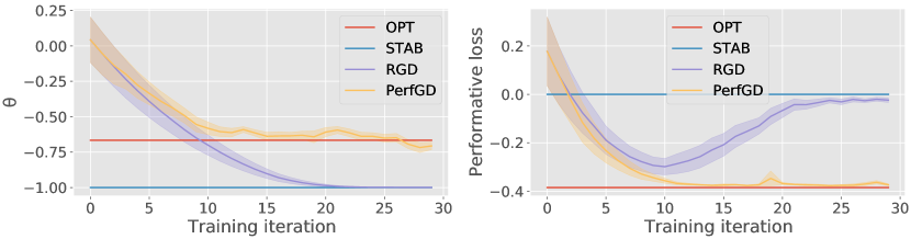
Figure 1: PerfGD vs. RGD for a modified version of the toy example introduced in Section 2.2. OPT denotes the performatively optimal point $\theta_{\mathrm{OPT}}$, and STAB denotes the performatively stable point $\theta_{\mathrm{STAB}}$. We set $\mu(\theta)=\sqrt{a_{1}\theta+a_{0}}$. Since the mean is nonlinear in $\theta$, estimating $d\mu/d\theta$ with finite differences is more challenging. In spite of this, PerfGD still converges to the optimal point.

For the second example, we set $\mathcal{D}(\theta)=\gamma\mathcal{N}(\mu_{1}(\theta),\sigma_{1}^{2})+(1-\gamma)\mathcal{N}(\mu_{2}(\theta),\sigma_{2}^{2})$. Here both of the means are linear in $\theta$, i.e. $\mu_{i}(\theta)=a_{i,1}\theta+a_{i,0}$. We apply PerfGD where the true cluster assignment for each point are known; in this case, PerfGD converges to $\theta_{\mathrm{OPT}}$ exactly and achieves optimal performative loss. The results are shown in Figure 2 below.

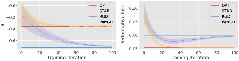
Figure 2: PerfGD vs. RGD for a modified version of the toy example introduced in Section 2.2 with a mixture of Gaussians. We supply the cluster label for each point. PerfGD is again able to converge to the minimum, while RGD converges to a suboptimal point.

5.2 Pricing

We next examine a generalized version of the problem introduced in Section 2.2. Let $\theta$ denote a vector of prices for various goods which we, the distributor, set. A vector $z$ denotes a customer’s demand for each good. Our goal is to maximize our expected revenue $\mathbb{E}_{\mathcal{D}(\theta)}[\theta^{\top}z]$. (In other words, we set the loss function $\ell(z;\theta)=-\theta^{\top}z$.) Assuming $\mathcal{D}(\theta)=\mathcal{N}(\mu(\theta),\Sigma)$, we can directly apply Algorithm 3 with the functions $\hat{\mu}$ and $\hat{\nabla}\mathcal{L}_{2}$ defined at the beginning of the section to compute the optimal prices.

Experiments

For this experiment, we work in a higher dimensional setting with $d=5$. We define $\Theta=[0,5]^{d}$ and $\mu(\theta)=\mu_{0}-\varepsilon\theta$. (That is, the mean demand for each good decreases linearly as the price increases.)

Our results are shown in Figure 3. For this case, we can compute $\theta_{\mathrm{OPT}}$ and $\theta_{\mathrm{STAB}}$ analytically. The performative revenue for each of these points is shown on the right side of the figure. As expected, PerfGD converges smoothly to the optimal prices, while RGD converges to the only fixed point which produces suboptimal revenue. In this case, RRM (not shown) stays fixed at $\theta_{\mathrm{RRM}}=[5,5,\ldots,5]^{\top}$.

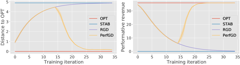
Figure 3: PerfGD vs. RGD for performative pricing. By taking into account the change in distribution, PerfGD converges to a set of prices which yields higher revenue than RGD. RRM (not shown) stays fixed at $\theta_{\mathrm{RRM}}=5\cdot\textbf{1}$, i.e. the vector with all entries equal to 5. Note that PerfGD follows RGD for the first several steps as part of the initialization phase. After this phase, the accurate estimate for the second part of the performative gradient allows PerfGD to reverse trajectory towards $\theta_{\mathrm{OPT}}$.

5.3 Binary classification

Suppose our goal is to predict a label $y\in\{0,1\}$ using features $x\in\mathbb{R}^{d}$. We assume that the label $y\sim\mathrm{Bernoulli}(\gamma)$, and that $x|y\sim\mathcal{N}(\mu^{y}(\theta),\Sigma_{y})$. The performative loss can then be written as

$$\mathcal{L}(\theta)=(1-\gamma)\mathbb{E}_{\mathcal{N}(\mu^{0}(\theta),\Sigma_{0})}[\ell(x,0;\theta)]+\gamma\mathbb{E}_{\mathcal{N}(\mu^{1}(\theta),\Sigma_{1})}[\ell(x,1;\theta)]$$ (5)

We can apply the general PerfGD method to each of the terms in (5) to obtain an approximate stochastic gradient. (We treat the features of the data with label $y=0$ as the dataset for the first term, and the features of the data with label $y=1$ as the dataset for the second term.)

Experiments

Here we work with a synthetic model of the spam classification example. We will classify emails with a logistic model, and we will allow a bias term. (That is, our model parameters $\theta=(\theta_{0},\theta_{1})^{\top}\in\mathbb{R}^{2}$. Given a real-valued feature $x$, our model outputs $h_{\theta}(x)=1/(1+e^{-\theta_{0}-\theta_{1}x})$.) We let the label $y=\mathbbm{1}\{\textrm{email is spam}\}$. For this case we assume that the distribution of the feature given the label is the performative aspect of the distribution map: spammers will try to alter their emails to slip past the spam filter, while people who use email normally will not alter their behavior according to the spam filter. To this end, we suppose that

$$x|y=0,\theta\sim\mathcal{N}(\mu_{0},\sigma_{0}^{2}),\hskip 18.06749ptx|y=1,\theta\sim\mathcal{N}(f(\theta),\sigma_{1}^{2}).$$

We note that assuming Gaussian features is in fact a realistic assumption in this case. Indeed, [LZH⁺20] shows that state-of-the-art performance on various NLP tasks can be achieved by transforming standard BERT embeddings so that they look like a sample from an isotropic Gaussian.

For this experiment, we set $f(\theta)=\mu_{1}-\varepsilon\theta_{1}$. Such a distribution map arises from the strategic classification setting described in [PZMDH20] in which the spammers optimize a non-spam classification utility minus a quadratic cost for changing their features. We use ridge-regularized cross-entropy loss for $\ell$.

Our results are shown in Figure 4. The improved estimate of the performative gradient given by PerfGD results in roughly a $9\%$ reduction in the performative loss over RGD. In this case, RRM (not shown) oscillates between two values of $\theta$ which both give significantly higher performative loss than either RGD or PerfGD.

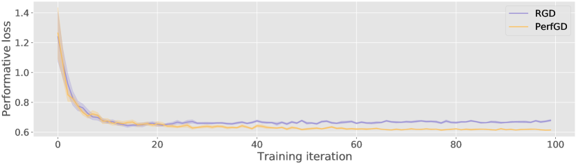
Figure 4: PerfGD vs. RGD for performative logistic regression. By taking into account the change in distribution, PerfGD is able to achieve a lower performative loss than RGD.

5.4 Regression

This setting is essentially a generalized version of the performative mean estimation problem in [PZMDH20]. For simplicity, assume that the marginal distribution of $x$ is independent of $\theta$. Assuming that $y|x\sim\mathcal{N}(\mu(x,\theta),\sigma^{2})$, the performative loss becomes

$$\mathcal{L}(\theta)=\mathbb{E}_{x}[\mathbb{E}_{\mathcal{N}(\mu(x,\theta),\sigma^{2})}[\ell(x,y;\theta)]].$$ (6)

The inner expectation has the required form to apply PerfGD. However, since $x$ takes continuous values, we will in general have only one sample to approximate the inner expectation in (6), leading to heavily biased or innacurate estimates for the required quantities in (2). This leaves us with two options: we can either use techniques for debiasing the required quantities and apply PerfGD directly, or we can use a reparameterization trick and a modified version of PerfGD. Here we present the latter approach.

We assume that the response $y$ follows a linear model, i.e. $y=\beta(\theta)^{\top}x+\varepsilon$, $\varepsilon\sim\mathcal{N}(0,\sigma^{2})$. The performative loss can then be written as

$$\mathcal{L}(\theta)=\mathbb{E}_{x,\varepsilon}[\ell(x,\beta(\theta)^{\top}x+\varepsilon;\theta)].$$ (7)

Since we have removed the dependence of the distribution on $\theta$, we can easily compute the gradient:

$$\nabla\mathcal{L}(\theta)=\mathbb{E}_{\mathcal{D}(\theta)}[\nabla_{\theta}\ell(x,y;\theta)]+\mathbb{E}_{\mathcal{D}(\theta)}\left[\frac{\partial\ell}{\partial y}\frac{d\beta}{d\theta}^{\top}x\right].$$

We can first estimate $\beta$ via e.g. regularized ordinary least squares, then estimate $d\beta/d\theta$ via finite differences as in the general setting (2): $\frac{d\beta}{d\theta}\approx\Delta\beta(\Delta\theta)^{\dagger}$.

Experiments

For simplicity, we use one-dimensional linear regression parameters $\theta\in\mathbb{R}$. The feature $x$ is drawn from a fixed distribution $x\sim\mathcal{N}(\mu_{x},\sigma_{x}^{2})$, and the performative coefficient $\beta(\theta)$ of $y|x$ has the form $\beta(\theta)=a_{0}+a_{1}\theta$. We use ridge-regularized squared loss for $\ell$.

Our results are summarized in Figure 5. In this case, there is a large gap between $\theta_{\mathrm{OPT}}$ and $\theta_{\mathrm{STAB}}$. As expected, PerfGD converges smoothly to $\theta_{\mathrm{OPT}}$, while in this case both RGD and RRM converge to $\theta_{\mathrm{STAB}}$. The improvement of PerfGD over RGD and RRM results in a factor of more than an order of magnitude in reduction of the performative loss.

Figure 5: PerfGD vs. RGD for performative linear regression. Top: Model parameters vs. training iteration. Bottom: Performative loss vs. training iteration. As expected, RGD converges to the performatively stable point, but in this case the stable point is very far from the performative optimum. PerfGD converges to OPT and incurs a much lower performative loss than RGD.

6 Conclusion

In this paper, we addressed the setting of modeling when the data distribution reacts to the model’s parameters, i.e. performative distribution shift. We verified that existing algorithms meant to address this setting in general converge to a suboptimal point in terms of the performative loss. We then introduced a new algorithm, PerfGD, which computes a more accurate estimate for the performative gradient under some parametric assumptions on the performative distribution. We proved theoretical results on the accuracy of our gradient estimate as well as the convergence of the method, and confirmed via several empirical examples that PerfGD outperforms existing algorithms such as repeated gradient descent and repeated risk minimization. The accuracy and iteration requirement are both practically feasible, as many ML systems have regular updates every few days.

Finally, we suggest directions for further research. A natural direction for future work is the extension of our methods to nonparametric distributions. Another direction which may prove fruitful is to improve the estimation of the derivative $df/d\theta$. Finally, methods specifically tailored to deal with high-dimensional data are also of interest.

Throughout the following proofs, we use $\mathcal{O}(\cdot)$ to denote the leading order behavior of various quantities as $T$ (the total number of steps taken by the method) becomes large and $\delta$ (the size of the error in the estimate for $f$) becomes small. For simplicity, all proofs are in one dimension.

Appendix A Bounding the error of $\widehat{f^{\prime}}$

Before we prove Lemma 1 (bounding the error of the full performative gradient), we must first bound the error of our approximation to $f^{\prime}$. Let $f_{t}=f(\theta_{t})$, $f^{\prime}_{t}=f^{\prime}(\theta_{t})$, and define $\hat{f_{t}}$ and $\widehat{f^{\prime}_{t}}$ similarly.

Lemma 4.

Under the assumptions of Section 4, we have $|\widehat{f^{\prime}_{t}}-f^{\prime}_{t}|=\mathcal{O}\left(\frac{\delta}{g}\frac{1}{\eta}+MG\eta\right)$.

Proof.

By definition, we have

$$\widehat{f^{\prime}_{t}}=\frac{\hat{f}_{t+1}-\hat{f_{t}}}{\theta_{t+1}-\theta_{t}}=\frac{f_{t+1}-f_{t}}{\theta_{t+1}-\theta_{t}}+\frac{\varepsilon_{t+1}-\varepsilon_{t}}{\theta_{t+1}-\theta_{t}}.$$ (8)

By Taylor’s theorem, we have

$$f_{t+1}=f_{t}+f^{\prime}_{t}\cdot(\theta_{t+1}-\theta_{t})+\frac{1}{2}f^{\prime\prime}(\xi)(\theta_{t+1}-\theta_{t})^{2}\hskip 7.22743pt\Longrightarrow\hskip 7.22743ptf^{\prime}_{t}=\frac{f_{t+1}-f_{t}}{\theta_{t+1}-\theta_{t}}+\frac{1}{2}f^{\prime\prime}(\xi)(\theta_{t+1}-\theta_{t}),$$ (9)

where $\xi$ is some number between $\theta_{t}$ and $\theta_{t+1}$. Next, note that since $\theta_{t+1}=\theta_{t}-\eta\hat{\nabla}\mathcal{L}_{t}$ and $g\leq|\hat{\nabla}\mathcal{L}_{t}|\leq G$, we have $\eta g\leq|\theta_{t+1}-\theta_{t}|\leq\eta G$. Using this fact and combining equations (8) and (9), we find that

$$|\widehat{f^{\prime}_{t}}-f^{\prime}_{t}| \leq\frac{|\varepsilon_{t+1}|+|\varepsilon_{t}|}{\eta g}+\frac{1}{2}|f^{\prime\prime}(\xi)|\eta G$$

$$\leq\frac{2\delta}{g}\frac{1}{\eta}+\frac{MG}{2}\eta$$

where we have also used the assumption that $|f^{\prime\prime}(\xi)|\leq M$. This is the desired bound. ∎

Appendix B Proof of Lemma 1

Proof.

We write $|\hat{\nabla}\mathcal{L}_{t}-\nabla\mathcal{L}_{t}|\leq|\hat{\nabla}_{1}\mathcal{L}_{t}-\nabla_{1}\mathcal{L}_{t}|+|\hat{\nabla}_{2}\mathcal{L}-\nabla_{2}\mathcal{L}_{t}|$ and bound each term on the right-hand side separately. We begin by bounding the error on $\nabla_{1}\mathcal{L}$. We have

$$|\hat{\nabla}_{1}\mathcal{L}_{t}-\nabla_{1}\mathcal{L}_{t}| \leq\int|\nabla\ell(z;\theta)||p(z;\hat{f_{t}})-p(z;f_{t})|\,dz$$

$$\leq\ell_{\mathrm{max}}\int|p(z;\hat{f_{t}})-p(z;f_{t})|\,dz$$

$$\leq\ell_{\mathrm{max}}\bigg{(}\underbrace{\int_{|z-f_{t}|\leq R}|p(z;\hat{f_{t}})-p(z;f_{t})|\,dz}_{\mathrm{(A)}}+\underbrace{\int_{|z-f_{t}|>R}|p(z;\hat{f_{t}})|\,dz}_{\mathrm{(B)}}+\underbrace{\int_{|z-f_{t}|>R}|p(z;f_{t})|\,dz}_{\mathrm{(C)}}\bigg{)},$$ (10)

where for simplicity we assume that $\ell_{\mathrm{max}}\geq|\nabla\ell(z;\theta)|$ is also an upper bound on the derivative of the point loss, and for any $R>0$.

To bound (A), we bound the Lipschitz constant of $p$ in its second argument. It suffices to bound $\partial_{2}p$. Observe that

$$\partial_{2}p(z;w)=c(z-w)e^{-\frac{1}{2\sigma^{2}}(z-w)^{2}}.$$

Letting $x=z-w$ and $\alpha=\frac{1}{2\sigma^{2}}$, we want to bound the maximum of $xe^{-\alpha x^{2}}$. Taking the derivative with respect to $x$, this has critical points at $x=\pm\frac{1}{\sqrt{2\alpha}}$. Since $|\partial_{2}p(z;w)|\rightarrow 0$ as $w\rightarrow\pm\infty$ for any $z$, these critical points are global maxima for $|\partial_{2}p|$. Thus $\max|\partial_{2}p|=\mathcal{O}(1)$ and $p$ is $\mathcal{O}(1)$-Lipschitz in its second argument. It follows that

$$\mathrm{(A)}\leq\int c|\hat{f_{t}}-f_{t}|\,dz=\mathcal{O}(R\delta).$$

To bound (B), oberserve that

$$\mathrm{(B)} \leq\int_{|z-\hat{f_{t}}|+|\hat{f_{t}}-f_{t}|>R}|p(z;\hat{f_{t}})|\,dz$$

$$\leq\int_{|z-\hat{f_{t}}|>R-\delta}|p(z;\hat{f_{t}})|\,dz$$

$$=\mathbb{P}_{\mathcal{N}(\hat{f_{t}},\sigma^{2})}(|z-\hat{f_{t}}|>R-\delta)$$

$$\leq 2e^{-(R-\delta)^{2}/2\sigma^{2}}$$

for any $R\geq\delta$. A similar calculation shows that (C) $\leq 2e^{-R^{2}/2\sigma^{2}}\leq 2e^{-(R-\delta)^{2}/2s^{2}}$ for $R\geq\delta$. Thus

$$\mathrm{(A)}+\mathrm{(B)}+\mathrm{(C)}=\mathcal{O}\left(R\delta+\exp\left(-\frac{(R-\delta)^{2}}{2\sigma^{2}}\right)\right)$$

for any $R\geq\delta$. Setting $R=\delta+\sqrt{2\sigma^{2}\log\frac{1}{\delta}}$ and substituting our bound back into (10), we obtain

$$|\hat{\nabla}_{1}\mathcal{L}_{t}-\nabla_{1}\mathcal{L}_{t}|=\mathcal{O}\left(\ell_{\mathrm{max}}\left(\delta\sqrt{\log\frac{1}{\delta}}\right)\right).$$ (11)

Next we bound the error $|\hat{\nabla}_{2}\mathcal{L}_{t}-\nabla_{2}\mathcal{L}_{t}|$. We have

$$|\hat{\nabla}_{2}\mathcal{L}_{t}-\nabla_{2}\mathcal{L}_{t}| =\left|\int\ell(z;\theta_{t})\partial_{2}p(z;\hat{f_{t}})\widehat{f^{\prime}_{t}}\,dz-\int\ell(z;\theta_{t})\partial_{2}p(z;f_{t})f^{\prime}_{t}\,dz\right|$$

$$\leq\underbrace{\int|\ell(z;\theta_{t})||\partial_{2}p(z;\hat{f_{t}})||\widehat{f^{\prime}_{t}}-f^{\prime}_{t}|\,dz}_{\mathrm{(I)}}+\underbrace{\int|\ell(z;\theta_{t})||\partial_{2}p(z;\hat{f_{t}})-\partial_{2}p(z;f_{t})||f^{\prime}_{t}|\,dz}_{\mathrm{(II)}}.$$ (12)

We proceed to bound the terms (I) and (II) separately.

The bound for (I) is straightforward. Recall that $|\ell(z;\theta_{t})|\leq\ell_{\mathrm{max}}$ and $\widehat{f^{\prime}_{t}}$ and $f^{\prime}_{t}$ are independent of $z$, so we have

$$\mathrm{(I)}\leq\ell_{\mathrm{max}}|\widehat{f^{\prime}_{t}}-f^{\prime}_{t}|\int|\partial_{2}p(z;\hat{f_{t}})|\,dz.$$

Since $p(z;\hat{f_{t}})$ is the pdf for a Gaussian with mean $\hat{f_{t}}$ and variance $\sigma^{2}$, a standard computation reveals that $\int|\partial_{2}p(z;\hat{f_{t}})|\,dz=\sqrt{\frac{2}{\pi\sigma^{2}}}=\mathcal{O}(1)$. Using the bound on $|\widehat{f^{\prime}_{t}}-f^{\prime}_{t}|$ from Lemma 4, we have

$$\mathrm{(I)}=\mathcal{O}\left(\ell_{\mathrm{max}}\left(MG\eta+\frac{\delta}{g}\frac{1}{\eta}\right)\right).$$ (13)

Next, we bound (II). First, since $|\ell(z;\theta_{t})|\leq\ell_{\mathrm{max}}$ and $|f^{\prime}_{t}|\leq F$, we have

$$\mathrm{(II)}\leq\ell_{\mathrm{max}}F\int|\partial_{2}p(z;\hat{f_{t}})-\partial_{2}p(z;f_{t})|\,dz$$ (14)

so it suffices to bound the integrand in (14).

For any $R\geq\delta$, we have

$$\int|\partial_{2}p(z;\hat{f_{t}})-\partial_{2}p(z;f_{t})|\,dz=\underbrace{\int_{|z-f_{t}|\leq R}|\partial_{2}p(z;\hat{f_{t}})-\partial_{2}p(z;f_{t})|\,dz}_{\mathrm{(i)}}+\underbrace{\int_{|z-f_{t}|>R}|\partial_{2}p(z;\hat{f_{t}})-\partial_{2}p(z;f_{t})|\,dz}_{\mathrm{(ii)}}.$$

To bound (i), it suffices to bound the Lipschitz constant of $\partial_{2}p(z;w)$ in the second variable (if one exists). We can do this by bounding $|\partial_{2}^{2}p|$. A direct computation shows that

$$\partial_{2}^{2}p(z;w)=\frac{1}{\sigma^{2}\sqrt{2\pi\sigma^{2}}}e^{-\frac{1}{2\sigma^{2}}(z-w)^{2}}\left(\frac{1}{\sigma^{2}}(z-w)^{2}-1\right).$$ (15)

Let $\alpha=\sigma^{-2}$ and $x=(z-w)^{2}$. Bounding (15) is equivalent to upper bounding an expression of the form $e^{-\frac{\alpha}{2}x}(\alpha x-1)$ over $x\geq 0$. Taking a derivative with respect to $x$ shows that the only critical point is at $x=2e^{-3/2}$; the only other point to check is the boundary point $x=0$. Checking both of these manually shows that the absolute value is maximized at $x=0$, and we obtain the bound

$$|\partial_{2}^{2}p(z;w)|\leq\frac{1}{\sigma^{2}\sqrt{2\pi\sigma^{2}}}=\mathcal{O}(1),$$

i.e. $\partial_{2}p(z;w)$ is $\mathcal{O}(1)$-Lipschitz in $w$. Applying this fact to (i), we have

$$\mathrm{(i)}\leq\int_{|z-f_{t}|\leq R}c|\hat{f_{t}}-f_{t}|\,dz=c\int_{|z-f_{t}|\leq R}|\varepsilon_{t}|\,dz=\mathcal{O}(R\delta).$$ (16)

Next we turn our attention to (ii). We have

$$\mathrm{(ii)} \leq\int_{|z-f_{t}|>R}|\partial_{2}p(z;\hat{f_{t}})|\,dz+\int_{|z-f_{t}|>R}|\partial_{2}p(z;f_{t})|\,dz$$

$$\leq\int_{|z-(f_{t}+\varepsilon_{t})|>R-|\varepsilon_{t}|}|\partial_{2}p(z;\hat{f_{t}})|\,dz+\int_{|z-f_{t}|>R}|\partial_{2}p(z;f_{t})|\,dz$$

$$\leq\int_{|z-f^{\prime}_{t}|>R-\delta}|\partial_{2}p(z;\hat{f_{t}})|\,dz+\int_{|z-f_{t}|>R}|\partial_{2}p(z;f_{t})|\,dz.$$ (17)

These inequalities follow from several applications of the triangle inequality and the bound $|\varepsilon_{t}|\leq\delta$. Now since $p(z;w)$ is a Gaussian pdf, we have $\partial_{2}p(z;w)=\frac{1}{\sigma^{2}}(z-w)p(z;w)$, and therefore

$$\int_{|z-w|>r}|\partial_{2}p(z;w)|\,dz =\int_{|z-w|>r}\frac{1}{\sigma^{2}}|z-w|p(z;w)\,dz$$

$$=\mathbb{E}_{\mathcal{N}(w,\sigma^{2})}\left[\mathbbm{1}\{|z-w|\geq r|\}\sigma^{-2}|z-w|\right]$$

$$\leq\sqrt{\mathbb{E}[\mathbbm{1}\{|z-w|\geq r\}^{2}]\sigma^{-2}\mathbb{E}[|z-w|^{2}]}$$ (18)

$$=\sqrt{\mathbb{P}(|z-w|\geq r)}$$

$$\leq\sqrt{2}e^{-\frac{r^{2}}{4\sigma^{2}}},$$ (19)

where (18) follows from the Cauchy-Schwarz inequality and (19) follows from a standard Gaussian tail bound. Applying (19) to (17), we obtain

$$\mathrm{(ii)} \leq c\left(\exp\left(-\frac{(R-\delta)^{2}}{4\sigma^{2}}\right)+\exp\left(-\frac{R^{2}}{4\sigma^{2}}\right)\right)$$

$$=\mathcal{O}\left(\exp\left(-\frac{(R-\delta)^{2}}{4\sigma^{2}}\right)\right)$$ (20)

for any $R\geq\delta$. Combining the bound (16) on (i) and (20) on (ii) with (14), we have

$$\mathrm{(II)}=\mathcal{O}\left(\ell_{\mathrm{max}}F\left[R\delta+\exp\left\{-\frac{(R-\delta)^{2}}{4\sigma^{2}}\right\}\right]\right).$$ (21)

If we take $R=\delta+\sqrt{4\sigma^{2}\log(1/\delta)}$ and substitute into (21), we obtain

$$\mathrm{(II)}=\mathcal{O}\left(\ell_{\mathrm{max}}F\delta\sqrt{\log(1/\delta)}\right).$$ (22)

We now substitute our bounds on (I) and (II) into (12), which yields

$$|\nabla_{2}\mathcal{L}-\hat{\nabla}_{2}\mathcal{L}|\leq\mathcal{O}\left(\ell_{\mathrm{max}}\left[MG\eta+\frac{\delta}{g}\frac{1}{\eta}+F\delta\sqrt{\log(1/\delta)}\right]\right).$$ (23)

To conlude, observe that the bound on the error of $\nabla_{1}\mathcal{L}_{t}$ in (11) can be completely absorbed into (23), and we obtain the desired result. ∎

Appendix C Proof of Theorem 2

Proof.

To simplify notation, we will let $L=L_{\mathrm{Lip}}$; this should not be confused with the decoupled performative loss function $L(\theta_{1},\theta_{2})$ defined in Section 2. Let $\mathcal{L}_{t}=\mathcal{L}(\theta_{t})$ and let $E_{t}=\hat{\nabla}\mathcal{L}_{t}-\nabla\mathcal{L}_{t}$. Since $\mathcal{L}$ is $L$-smooth and convex, we have the standard inequality

$$\mathcal{L}_{t+1}\leq\mathcal{L}_{t}+\nabla\mathcal{L}_{t}\cdot(\theta_{t+1}-\theta_{t})+\frac{L}{2}|\theta_{t+1}-\theta_{t}|^{2}.$$ (24)

Since $\theta_{t+1}-\theta_{t}=\eta\hat{\nabla}\mathcal{L}_{t}$, we can rewrite (24):

$$\mathcal{L}_{t+1}\leq\mathcal{L}_{t}+\eta(|\nabla\mathcal{L}_{t}||E_{t}|-|\nabla\mathcal{L}_{t}|^{2})+\eta^{2}L(|\nabla\mathcal{L}_{t}|^{2}+|E_{t}|^{2})$$ (25)

Rearranging and using the fact that $|\nabla\mathcal{L}_{t}|\leq G$, we have

$$(\eta-\eta^{2}L)|\nabla\mathcal{L}_{t}|^{2}\leq\mathcal{L}_{t}-\mathcal{L}_{t+1}+\eta G|E_{t}|+\eta^{2}L|E_{t}|^{2}.$$ (26)

If we sum both sides of (26) from $t=1$ to $T$, we find that

$$T\min_{1\leq t\leq T}|\nabla\mathcal{L}_{t}|^{2}\leq\sum_{t=1}^{T}|\nabla\mathcal{L}_{t}|^{2}\leq\frac{\mathcal{L}_{1}-\mathcal{L}_{T+1}+\eta G\sum_{t=1}^{T}|E_{t}|+\eta^{2}L\sum_{t=1}^{T}|E_{t}|^{2}}{\eta-L\eta^{2}}.$$ (27)

Note that with $\eta=\sqrt{\frac{1}{MG^{2}T}+\frac{\delta}{MGg}}$ as specified by the theorem, we have $\eta^{2}=o(\eta)$. Furthermore, by Lemma 1, we have

$$|E_{t}|=\mathcal{O}\left(\ell_{\mathrm{max}}\sqrt{\frac{M}{T}+\frac{MG\delta}{g}}\right)\equiv\mathbf{E}.$$ (28)

(In obtaining the above bound, we have assumed WLOG that $G\geq 1$.) Note that since $\mathbf{E}=o(1)$, we have $\mathbf{E}^{2}=o(\mathbf{E})$. Lastly, since $\mathcal{L}_{t}=\mathbb{E}_{p(z;\theta_{t})}[\ell(z;\theta_{t})]$ we have $|\mathcal{L}_{t}|\leq\ell_{\mathrm{max}}$ for all $t$. Applying these facts to (27), we have

$$\min_{1\leq t\leq T}|\nabla\mathcal{L}_{t}|^{2} =\mathcal{O}\left(\frac{\ell_{\mathrm{max}}+\eta GT\mathbf{E}+\eta^{2}LT\mathbf{E}^{2}}{T\eta}\right)$$

$$=\mathcal{O}\left(\frac{\ell_{\mathrm{max}}}{T\eta}+G\ell_{\mathrm{max}}\left[MG\eta+\frac{\delta}{g}\frac{1}{\eta}\right]\right)$$

$$=\mathcal{O}\left(\ell_{\mathrm{max}}\sqrt{\frac{MG^{2}}{T}+\frac{MG^{3}\delta}{g}}\right)$$ (29)

where the last equation follows from our choice of $\eta$.

Lastly, recall that our bound on $|E_{t}|$ required that $|\hat{\nabla}\mathcal{L}_{t}|\geq g$ for all $1\leq t\leq T$. If at any point we have $|\hat{\nabla}\mathcal{L}_{t}|<g$, then we can terminate and return this iterate. But then we have

$$|\nabla\mathcal{L}_{t}|^{2} \leq 2|\hat{\nabla}\mathcal{L}_{t}|^{2}+2|E_{t}|^{2}$$

$$\leq\mathcal{O}(g^{2}+\mathbf{E}^{2}).$$ (30)

Note that $\varepsilon_{*}\equiv\mathbf{E}^{2}=\mathcal{O}\left(\ell_{\mathrm{max}}^{2}\left(\frac{M}{T}+\frac{MG\delta}{g}\right)\right)=(T^{-1}+\delta)\cdot\mathcal{O}(\textrm{poly}(\ell_{\mathrm{max}},M,G,g^{-1})$ as specified in the statement of Theorem 2. We can guarantee that PerfGD reaches at least the max of the two bounds (29) and (30), yielding the desired result.

∎

We remark that, for a given accuracy level $\delta$, we should take a time horizon $T\propto\delta^{-1}$. Increasing $T$ beyond this point will not cause the error bound from Theorem 2 to decay any further.

Appendix D Convergence of PerfGD with stochastic errors and general $H$

When the errors on the estimate for $f$ are bounded and deterministic, we gain no advantage by increasing the length of the estimation horizon $H$. However, when the errors are centered and stochastic, the estimation horizon now plays a critical roll. Increasing $H$ allows for concentration of the errors, leading to overall better estimates for $f$. At the same time, increasing $H$ causes the deterministic bias from our finite difference approximations to increase. In the following section, we show how to balance these two factors and choose an optimal $H$. First, we state our main theorem.

Theorem 5.

With step size

$$\eta=\frac{g^{2/3}}{M^{1/2}G^{5/3}\tau^{1/3}(\log\frac{T}{\gamma})^{1/6}T^{5/6}}$$

and estimation horizon

$$H=\frac{\tau^{2/5}(\log\frac{T}{\gamma})^{1/5}}{M^{2/5}g^{4/5}}\eta^{-4/5}$$

the iterates of PerfGD satisfy

$$\min_{1\leq t\leq T}|\nabla\mathcal{L}_{t}|^{2}=\max\left\{\mathcal{O}\left(\ell_{\mathrm{max}}\left[\frac{1}{T^{1/6}}\cdot\frac{M^{1/2}G^{5/3}\tau^{1/3}(\log\frac{T}{\gamma})^{1/6}}{g^{2/3}}\right]\right),\mathcal{O}(g^{2}+\tau^{c_{1}}T^{-c_{2}}\cdot\mathrm{poly}(M,G,\gamma^{-1},g^{-1}))\right\}$$

with probability at least $1-\mathcal{O}(\gamma)$ as $\tau\rightarrow 0$ and $T\rightarrow\infty$ and for some positive constants $c_{1},c_{2}$.

We remark briefly that we choose to analyze $\tau\rightarrow 0$ since if the estimates for $f_{t}$ are computed from random samples of increasing size, then we expect the variance of these estimates (measured by $\tau$) to decay to zero as the sample size $n\rightarrow\infty$. For instance, for estimating the mean of a Gaussian we will have $\tau^{2}=\mathcal{O}(1/n)$.

The proof of Theorem 5 follows from two key lemmas.

Lemma 6.

If $X$ is $\tau^{2}$-subgaussian and $Y$ is any random variable with $|Y|\leq B$ w.p. 1, then $XY$ is $B^{2}\tau^{2}$-subgaussian.

A critical fact about this lemma is that the random variables involved need not be independent.

Proof.

By definition, $Z$ is $s^{2}$-subgaussian if $\mathbb{E}e^{Z^{2}/s^{2}}\leq 2$. Observe that since the exponential function is monotonic, we have

$$\mathbb{E}e^{X^{2}Y^{2}/B^{2}\tau^{2}}\leq\mathbb{E}e^{X^{2}B^{2}/B^{2}\tau^{2}}=\mathbb{E}e^{X^{2}/\tau^{2}}\leq 2.$$

Thus $XY$ is $B^{2}\tau^{2}$-subgaussian.

∎

Lemma 7.

We have $\widehat{f^{\prime}_{t}}=f_{t}^{\prime}+b_{t}+e_{t}$, where $b_{t}$ is a deterministic bias term with $|b_{t}|=\mathcal{O}(MGH\eta)$. Under the additional assumption that $\theta_{t}$ converge monotonically, $e_{t}$ is $\mathcal{O}\left(\frac{G^{2}\tau^{2}}{H^{3}g^{4}\eta^{2}}\right)$-subgaussian.

Proof.

The pseudoinverse used to compute $\widehat{f^{\prime}_{t}}$ is equivalent to solving the least-squares problem

$$\widehat{f^{\prime}_{t}}=\operatorname*{argmin}_{\alpha}\frac{1}{2}\sum_{i=1}^{H}(\alpha(\theta_{t-i}-\theta_{t})-(\hat{f}_{t-i}-\hat{f_{t}}))^{2}\hskip 7.22743pt\Longrightarrow\hskip 7.22743pt\widehat{f^{\prime}_{t}}=\frac{\sum_{i=1}^{H}(\hat{f}_{t-i}-\hat{f_{t}})(\theta_{t-i}-\theta_{t})}{\sum_{i=1}^{H}(\theta_{t-i}-\theta_{t})^{2}}.$$ (31)

Writing $\hat{f_{t}}=f_{t}+\varepsilon_{t}$ with $\varepsilon_{t}$ $\tau$-subgaussian, we can apply Taylor’s theorem to rewrite

$$\hat{f}_{t-i}-\hat{f_{t}}=f^{\prime}_{t}(\theta_{t-i}-\theta_{t})+\frac{1}{2}f^{\prime\prime}(\xi_{i})(\theta_{t-i}-\theta_{t})^{2}+\varepsilon_{t-i}-\varepsilon_{t}.$$ (32)

Using the explicit solution in (31) and substituting (32) for $\hat{f}_{t-i}-\hat{f_{t}}$, we find that

$$|\widehat{f^{\prime}_{t}}-f^{\prime}_{t}|\leq\underbrace{\frac{\frac{1}{2}\sum_{i=1}^{H}|f^{\prime\prime}(\xi_{i})||\theta_{t-i}-\theta_{t}|^{3}}{\sum_{i=1}^{H}(\theta_{t-i}-\theta_{t})^{2}}}_{b_{t}}+\underbrace{\frac{\sum_{i=1}^{H}(\varepsilon_{t-i}-\varepsilon_{t})(\theta_{t-i}-\theta_{t})}{\sum_{i=1}^{H}(\theta_{t-i}-\theta_{t})^{2}}}_{e_{t}}.$$

To bound $b_{t}$, observe that since $\theta_{t}=\theta_{t-i}-\eta(\hat{\nabla}\mathcal{L}_{t-i}+\cdots+\hat{\nabla}\mathcal{L}_{t-1})$ and $|\hat{\nabla}\mathcal{L}_{s}|\leq G$ and $i\leq H$, we have $|\theta_{t-i}-\theta_{t}|\leq HG\eta$ for all $i,t$. Since $|f^{\prime\prime}(\xi_{i})|\leq M$, we have

$$|b_{t}| \leq\frac{\frac{1}{2}\sum_{i=1}^{H}MHG\eta(\theta_{t-i}-\theta_{t})^{2}}{\sum_{i=1}^{H}(\theta_{t-i}-\theta_{t})^{2}}$$

$$=\mathcal{O}(MGH\eta).$$

Next we bound $e_{t}$. Since we have assumed that $\theta_{t}$ converge monotonically and $|\hat{\nabla}\mathcal{L}_{t}|\geq g$, we have

$$\frac{1}{\sum_{i=1}^{H}(\theta_{t-i}-\theta_{t})^{2}}\leq\frac{1}{\sum_{i=1}^{H}(ig\eta)^{2}}=\mathcal{O}(\frac{1}{H^{3}g^{2}\eta^{2}}).$$

In the numerator, we have

$$|\sum_{i=1}^{H}(\varepsilon_{t-i}-\varepsilon_{t})(\theta_{t-i}-\theta_{t})|\leq HG\eta\sum_{i=1}^{H}|\varepsilon_{t-i}-\varepsilon_{t}|.$$

Combining these, we have

$$e_{t}=\mathcal{O}\left(\frac{G}{H^{2}g^{2}\eta}\right)\sum_{i=1}^{H}|\varepsilon_{t-i}-\varepsilon_{t}|.$$ (33)

We make the additional simplifying assumption that the $|\varepsilon_{t-i}-\varepsilon_{t}|$ are independent. We can accomplish this splitting our dataset drawn from $\mathcal{D}(\theta_{t})$ into $H$ parts and estimating $f_{t}$ once with each component, then replacing the terms $(\hat{f}_{t-i}-\hat{f_{t}})$ with $(\hat{f}_{t-i}-\hat{f}_{t,i})$ in equation (31), where $\hat{f}_{t,i}$ is the estimate of $f_{t}$ from the $i$-th partition of the dataset. The errors $\varepsilon_{t}$ in the expression for $e_{t}$ now become independent copies $\varepsilon_{t,i}$, and the terms in equation (33) are indeed independent.

Under this assumption, $|\varepsilon_{t-i}-\varepsilon_{t,i}|$ are independent $2\tau^{2}$-subgaussian random variables. Their sum is therefore $\sum_{i=1}^{H}2\tau^{2}=\mathcal{O}(H\tau^{2})$-subgaussian. Finally, by Lemma 6, it follows that $e_{t}$ is $\mathcal{O}(\frac{G^{2}\tau^{2}}{H^{3}g^{4}\eta^{2}})$-subgaussian.

∎

With these two lemmas, we can now prove the main theorem. The structure of the proof is similar to that of Theorem 2.

Proof of Theorem 5.

We first establish a high-probability bound on $|e_{t}|$. By the subgaussian tail bound and a union bound over $t=1$ to $T$, a simple calculation shows that

$$|e_{t}|=\mathcal{O}\left(\frac{G\tau\sqrt{\log\frac{T}{\gamma}}}{g^{2}\eta H^{3/2}}\right)$$

with probability at least $1-\gamma$ for all $t=1,\ldots,T$. Combining this bound with the bound on $|b_{t}|$ from Lemma 7, we find that

$$|\widehat{f^{\prime}_{t}}-f^{\prime}_{t}|=\mathcal{O}\left(MG\eta H+\frac{G\tau\sqrt{\log\frac{T}{\gamma}}}{g^{2}\eta}H^{-3/2}\right).$$

With $H$ chosen as is in the theorem, this bound simplifies to

$$|\widehat{f^{\prime}_{t}}-f^{\prime}_{t}|=\mathcal{O}\left(\frac{M^{3/5}G\tau^{2/5}(\log\frac{T}{\gamma})^{1/5}}{g^{4/5}}\eta^{1/5}\right)\equiv\mathbf{E}_{1}.$$ (34)

From the proof of Lemma 1, we know that

$$|\hat{\nabla}\mathcal{L}_{t}-\nabla\mathcal{L}_{t}|=\mathcal{O}\left(\ell_{\mathrm{max}}\left[\mathbf{E}_{1}+F\delta\sqrt{\log\frac{1}{\delta}}\right]\right),$$ (35)

where $\delta$ is a (high-probability) bound on the error of $f_{t}$. Again assuming that this error is $\tau^{2}$-subgaussian, we have that

$$(\textrm{error on }f_{t})=\mathcal{O}\left(\tau\sqrt{\log\frac{T}{\gamma}}\right)$$

for all $t=1,\ldots,T$ with probability at least $1-\gamma$. Thus we can take $\delta=\tau\sqrt{\log(T/\gamma)}$, in which case the second term in equation (35) is $\mathcal{O}(\mathbf{E}_{1})$ as $\tau\downarrow 0$. It follows that $|\hat{\nabla}\mathcal{L}_{t}-\nabla\mathcal{L}_{t}|=\mathcal{O}(\ell_{\mathrm{max}}\mathbf{E}_{1})\equiv\mathbf{E}_{2}$ with high probability.

Finally, by the same analysis used in the proof of Theorem 2, we have that

$$\min_{1\leq t\leq T}|\nabla\mathcal{L}_{t}|^{2}=\mathcal{O}\left(\frac{\ell_{\mathrm{max}}+\eta GT\mathbf{E}_{2}}{T\eta}\right).$$

Choosing $\eta$ as in the theorem statement and substituting our bound on $\mathbf{E}_{2}$ yields the desired result. The max in the theorem statement follows from the same logic as in Theorem 2 plus the bound on the error performative gradient error $\mathbf{E}_{2}$. ∎

Appendix E Experiment details

In all of the following experiments, whenever the stated estimation horizon $H$ is longer than the entire history on a particular iteration of PerfGD, we simply use $H=$ length of the existing history for that iteration instead. Furthermore, in all of the experiments, both RGD and PerfGD were run using a learning rate of $\eta=0.1$.

E.1 Mixture of Gaussians and nonlinear mean (§5.1)

For the nonlinear mean experiment, we set $a_{0}=a_{1}=1$ and $\sigma^{2}=1$. At each iteration, we drew $n=500$ data points. We initialized PerfGD using only one step of RGD, and at each step after the initialization we used the previous $H=4$ steps to estimate $\mu^{\prime}(\theta)$. The analytical values for $\theta_{\mathrm{OPT}}$ and $\theta_{\mathrm{STAB}}$ are given by

$$\theta_{\mathrm{OPT}}=-\frac{2a_{0}}{3a_{1}},\hskip 18.06749pt\theta_{\mathrm{STAB}}=-\frac{a_{0}}{a_{1}}.$$

For the Gaussian mixture experiment, we set $\gamma=0.5$, $\sigma_{1}^{2}=1$, $a_{1,0}=-0.5$, $a_{1,1}=1$, $s_{2}^{2}=0.25$, $a_{2,0}=1$, and $a_{2,1}=-0.3$. At each iteration, we drew $n=1000$ data points. We initialized PerfGD using only one step of RGD, and at each step after the initialization we use the entire history to estimate $\mu_{i}^{\prime}(\theta)$. The analytical values for $\theta_{\mathrm{OPT}}$ and $\theta_{\mathrm{STAB}}$ are given by

$$\theta_{\mathrm{OPT}}=-\frac{1}{2}\frac{\gamma a_{1,0}+(1-\gamma)a_{2,0}}{\gamma a_{1,1}+(1-\gamma)a_{2,1}},\hskip 18.06749pt\theta_{\mathrm{STAB}}=\frac{\gamma a_{1,0}+(1-\gamma)a_{2,0}}{\gamma a_{1,1}+(1-\gamma)a_{2,1}}.$$

E.2 Pricing (§5.2)

We set $d=5$ for this experiment. We then set $\mu_{0}=6\cdot\mathbf{1}+\mathrm{Unif}[0,1]^{5}$ with a fixed random seed; in this case, it came out to $\mu_{0}\approx[6.55,6.72,6.60,6.54,6.42]^{\top}$. We set $\Sigma=I\in\mathbb{R}^{5\times 5}$ (i.e. the $5\times 5$ identity matrix) and $\varepsilon=1.5$. At each iteration, we drew $n=500$ data points. We initialized PerfGD with 14 steps of RGD, and at each step after initialization we used the entire history to estimate $d\mu/d\theta$. The analytical values for $\theta_{\mathrm{OPT}}$ and $\theta_{\mathrm{STAB}}$ are given by

$$\theta_{\mathrm{OPT}}=\frac{\mu_{0}}{2\varepsilon},\hskip 18.06749pt\theta_{\mathrm{STAB}}=\frac{\mu_{0}}{\varepsilon}.$$

E.3 Binary classification (§5.3)

Here the features $x\in\mathbb{R}$ are one-dimensional, while our model parameters $\theta\in\mathbb{R}^{2}$ allow for a bias term. We set $\sigma_{0}^{2}=0.25$, $\mu_{0}=1$, $\sigma_{1}^{2}=0.25$, $\mu_{1}=-1$, and $\varepsilon=3$. The regularization strength for $\ell$ was $\lambda=10^{-2}$, i.e.

$$\ell(x,y;\theta)=-y\log h_{\theta}(x)-(1-y)\log(1-h_{\theta}(x))+\frac{10^{-2}}{2}\lVert\theta\rVert^{2}.$$

When approximating the derivatives of the means of the mixtures with respect to $\theta$, we assume that it is known that the derivative of the non-spam email mean is independent of $\theta$, and we also assume knowledge of the fact that the mean of the spam email features depends only on $\theta_{1}$ (i.e. the non-bias parameter). At each iteration, we drew $n=500$ data points. We initialize PerfGD using only one step of RGD, and at each step after the initialization we use the entire history to estimate $f^{\prime}(\theta)$.

E.4 Regression (§5.4)

We set $\mu_{x}=1.67$, $\sigma_{x}^{2}=1$, $a_{0}=a_{1}=1.67$, and regularization strength $\lambda=3.33$ for the loss, i.e.

$$\ell(x,y;\theta)=\frac{1}{2}(\theta x-y)^{2}+\frac{3.33}{2}|\theta|^{2}.$$

The variance of $y|x$ was set to $4.12$. At each iteration, we drew $n=500$ data points. The analytical values for $\theta_{\mathrm{OPT}}$ and $\theta_{\mathrm{STAB}}$ are given by

$$\theta_{\mathrm{OPT}}=\frac{c\cdot a_{0}}{c\cdot(1-a_{1})+\frac{\lambda}{1-a_{1}}},\hskip 18.06749pt\theta_{\mathrm{STAB}}=\frac{c\cdot a_{0}}{c\cdot(1-a_{1})+\lambda},$$

where $c=\mu_{x}^{2}+\sigma_{x}^{2}$.

References

- [AS20] Ahmad Ajalloeian and S. Stich. Analysis of sgd with biased gradient estimators. arXiv, 2008.00051, 2020.
- [BBK20] Daniel Björkegren, J. Blumenstock, and Samsun Knight. Manipulation-proof machine learning. arXiv, 2004.03865, 2020.
- [BGZ15] Omar Besbes, Yonatan Gur, and Assaf Zeevi. Non-stationary stochastic optimization. Operations Research, 63(5):1227–1244, 2015.
- [BHK20] G. Brown, Shlomi Hod, and Iden Kalemaj. Performative prediction in a stateful world. arXiv, 2011.03885, 2020.
- [BKS12] Michael Brückner, Christian Kanzow, and Tobias Scheffer. Static prediction games for adversarial learning problems. Journal of Machine Learning Research, 13:2617–2654, 2012.
- [BLWZ20] Yahav Bechavod, Katrina Ligett, Z. Wu, and Juba Ziani. Causal feature discovery through strategic modification. arXiv, 2002.07024, 2020.
- [BM03] D. Bergemann and S. Morris. Robust mechanism design. Yale: Cowles Foundation Working Papers, 2003.
- [CDP15] Yang Cai, Constantinos Daskalakis, and Christos Papadimitriou. Optimum statistical estimation with strategic data sources. In Journal of Machine Learning Research, volume 40, pages 1–17, 2015.
- [CLP20] Y. Chen, Yang Liu, and Chara Podimata. Learning strategy-aware linear classifiers. In NeurIPS, 2020.
- [CPPS18] Yiling Chen, Chara Podimata, Ariel D Procaccia, and Nisarg Shah. Strategyproof Linear regression in high dimensions. In ACM EC 2018 - Proceedings of the 2018 ACM Conference on Economics and Computation, pages 9–26, 2018.
- [DDM+04] Nilesh Dalvi, Pedro Domingos, Mausam, Sumit Sanghai, and Deepak Verma. Adversarial classification. In KDD-2004 - Proceedings of the Tenth ACM SIGKDD International Conference on Knowledge Discovery and Data Mining, pages 99–108, 2004.
- [DJWW15] John Duchi, Michael Jordan, Martin Wainwright, and Andre Wibisono. Optimal rates for zero-order convex optimization: The power of two function evaluations. IEEE Transactions on Information Theory, 61, 12 2015.
- [DX20] D. Drusvyatskiy and Lin Xiao. Stochastic optimization with decision-dependent distributions. arXiv, 2011.11173, 2020.
- [HMPW16] Moritz Hardt, Nimrod Megiddo, Christos Papadimitriou, and Mary Wootters. Strategic classification. In ITCS 2016 - Proceedings of the 2016 ACM Conference on Innovations in Theoretical Computer Science, pages 111–122, 2016.
- [KLMO15] Jon Kleinberg, Jens Ludwig, Sendhil Mullainathan, and Ziad Obermeyer. Prediction policy problems. In American Economic Review, volume 105, pages 491–495, 2015.
- [KR19] Jon Kleinberg and Manish Raghavan. How do classifiers induce agents to invest effort strategically? In ACM EC 2019 - Proceedings of the 2019 ACM Conference on Economics and Computation, pages 825–844, 2019.
- [KTS+19] Moein Khajehnejad, Behzad Tabibian, B. Schölkopf, A. Singla, and M. Gomez-Rodriguez. Optimal decision making under strategic behavior. arXiv, 1905.09239, 2019.
- [Lat20] Tor Lattimore. Improved regret for zeroth-order adversarial bandit convex optimisation. arXiv, 2006.00475, 2020.
- [LZH+20] Bohan Li, Hao Zhou, Junxian He, Mingxuan Wang, Yiming Yang, and Lei Li. On the sentence embeddings from pre-trained language models. In EMNLP, 2020.
- [MDPZH20] Celestine Mendler-Dünner, J. C. Perdomo, Tijana Zrnic, and M. Hardt. Stochastic optimization for performative prediction. NeurIPS, 2020.
- [MMH20] John Miller, Smitha Milli, and M. Hardt. Strategic classification is causal modeling in disguise. In ICML, 2020.
- [Mun20] Evan Munro. Learning to personalize treatments when agents are strategic. arXiv, 2011.06528, 2020.
- [PZMDH20] Juan Perdomo, Tijana Zrnic, Celestine Mendler-Dünner, and Moritz Hardt. Performative prediction. In ICML, 2020.
- [QCSSL09] Joaquin Quionero-Candela, Masashi Sugiyama, Anton Schwaighofer, and Neil D. Lawrence. Dataset Shift in Machine Learning. The MIT Press, 2009.
- [Sas08] Saskia Sassen. Do economists make markets? on the performativity of economics. American Journal of Sociology, 2008.
- [SEA20] Yonadav Shavit, Benjamin Edelman, and B. Axelrod. Learning from strategic agents: Accuracy, improvement, and causality. arXiv, 2002.10066, 2020.
- [Wil92] Ronald J. Williams. Simple statistical gradient-following algorithms for connectionist reinforcement learning. Machine Learning, 8(3):229–256, May 1992.