Structural reduction of chemical reaction networks
based on topology

Abstract

We develop a model-independent reduction method of chemical reaction systems based on the stoichiometry, which determines their network topology. A subnetwork can be eliminated systematically to give a reduced system with fewer degrees of freedom. This subnetwork removal is accompanied by rewiring of the network, which is prescribed by the Schur complement of the stoichiometric matrix. Using homology and cohomology groups to characterize the topology of chemical reaction networks, we can track the changes of the network topology induced by the reduction through the changes in those groups. We prove that, when certain topological conditions are met, the steady-state chemical concentrations and reaction rates of the reduced system are ensured to be the same as those of the original system. This result holds regardless of the modeling of the reactions, namely chemical kinetics, since the conditions only involve topological information. This is advantageous because the details of reaction kinetics and parameter values are difficult to identify in many practical situations. The method allows us to reduce a reaction network while preserving its original steady-state properties, thereby complex reaction systems can be studied efficiently. We demonstrate the reduction method in hypothetical networks and the central carbon metabolism of Escherichia coli.

I Introduction

Chemical reactions in living systems form complex networks [1, 2, 3]. They operate in a highly coordinated manner, and are responsible for various cellular functions. Experimentally, high-throughput measurements have been conducted to study cellular responses to perturbations for the purpose of elucidating underlying regulatory mechanisms (see, for example, Refs. [4, 5, 6]). One approach to the theoretical studies of biological systems is to build elaborated models, employing particular kinetics, parameter values, and initial/external conditions. Although these models can provide detailed quantitative predictions, a faithful modeling is challenging for most biological systems, because our prior knowledge about kinetics and parameter values is limited, and also because many parameters are difficult to measure experimentally. Furthermore, the complexity of models may confound model-independent features with model-dependent ones.

To address these difficulties, it is desirable to reduce complex reaction systems to simpler ones. A reduction is practically useful since it can reduce the number of variables and parameters needed to be included in the analysis, and it can also identify features essential to focal phenomena or properties of interest (such as biomass production of a metabolic network). It also relates to a conceptual question of the robustness of biochemical processes [7, 8, 9, 10, 11, 12, 13, 14]. Chemical reaction networks inside living organisms are highly interconnected, and yet are robust under internal fluctuations and environmental perturbations. If a system is insensitive to the details of its substructure, it is natural to expect that a reduction is possible, in the spirit of renormalization. To the best of our knowledge, the reduction methods [15, 16] of chemical reaction systems studied so far are based on timescale separation, lumping [17, 18], sensitivity analysis [19, 20, 21] or optimizations [22, 23]. To apply those approaches, we need detailed information about the reactions. For example, to exploit the timescale separation, we should know which reactions are fast and which are slow. The sensitivity analysis also requires the dependence of the system on various parameters.

In this paper, we develop a systematic method of reducing chemical reaction networks based on their topology (see Figs. 1 and 2). One motivation for the reduction method comes from the law of localization [24, 25, 26]; if a certain topological index, which we call the influence index, is zero for a subnetwork, perturbations inside the subnetwork do not affect the steady state of the remaining elements of the network (see Sec. III for the precise statement). This observation indicates that certain subnetworks are ‘irrelevant’, as far as the remaining part of the network is concerned. As we will show, a reduction can be systematically performed through the Schur complementation of the stoichiometric matrix with respect to a subset of chemical species and reactions. The well-definedness of the reduction process requires that the subnetwork should satisfy a condition called the output-completeness. The behavior of the reduced system depends on the topological nature of the subnetwork. As a central result, we prove that, when the influence index of the subnetwork vanishes, the steady-state chemical concentrations and reaction rates of the reduced system are exactly the same as those of the original system, as far as the remaining degrees of freedom are concerned.

We emphasize that those conditions are topological ones and determined solely by the network structure; hence, are insensitive to the details of how the reactions are modeled. Thus, the result is broadly applicable, because it holds regardless of the kinetics or parameter values. This is of practical merit since the kinetics of reactions or the values of parameters are difficult to identify in many situations. To characterize the topology of reaction networks, we introduce the homology and cohomology groups for chemical reaction networks. The change of the topology of chemical reaction networks under the reduction is captured by the change of the (co)homology groups. The tools of algebraic topology are convenient for tracking those changes. We recommend the readers who are interested in practical aspects of reduction to directly go to Sec. IV, where we discuss the reduction procedure with simple examples.

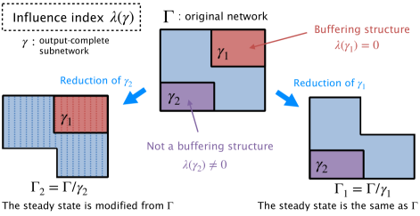
Figure 1: Schematic of the reduction procedure. For a given subnetwork $\gamma$ satisfying a condition called output-completeness, we assign a nonnegative integer that we call the influence index, $\lambda(\gamma)$. A subnetwork with vanishing influence index is called a buffering structure. Although an elimination of a subnetwork ($\gamma_{2}$ in the figure) generally modifies the steady state of the remaining part of the network, a buffering structure ($\gamma_{1}$) can be reduced while preserving the original steady state of the remaining part.

Figure 2: Example of the reduction. In a chemical reaction network with a stoichiometric matrix $S$, if a subnetwork $\gamma$ with $S_{\gamma}$ is output-complete, the system can be reduced to a smaller system, whose stoichiometric matrix $S^{\prime}$ is given by the generalized Schur complement $S^{\prime}\coloneqq S/S_{\gamma}$. The reduced system can reproduce the same steady-state properties of the original system, if the influence index of the subnetwork is zero. Note that $S^{\prime}$ is in general different from the corresponding submatrix of $S$ (compare the lower-right block of $S$ with $S^{\prime}$, where the difference between them is indicated by the colored components in $S^{\prime}$). This alteration is pictorially represented as ‘rewiring’ of the network (e.g., the head of $e_{5}$ is rewired to $v_{3}$). See Fig. 5 for an application to the central carbon metabolism of E. coli.

The rest of the paper is organized as follows. In Sec. II, we introduce concepts for characterizing the structure of chemical reaction networks. Further, we introduce the homology and cohomology groups for chemical reaction networks, and the steady-state reaction rates and concentrations are determined by the elements of the cohomology groups. In Sec. III, we review the structural sensitivity analysis and the law of localization. We also show that the influence index is submodular as a function over output-complete subnetworks. In Sec. IV, we introduce the reduction procedure and illustrate the method with simple examples. In Sec. V, we discuss the relation between the structural sensitivity analysis and the reduction method. We show that the reduction of a buffering structure, that is an output-complete subnetwork with vanishing influence index, has a particularly nice property: The reduced system admits the same steady states as the original system. In Sec. VI, as an application to realistic networks, we demonstrate the reduction method for the metabolic pathways of Escherichia coli. Section VII is devoted to summary and outlook. In Appendix A, we discuss the Hodge decomposition and Laplace operators for chemical reaction networks. In Appendix B, we provide intuitive interpretations of the cycles and conserved charges of various types that appear in the decomposition of the influence index. We also illustrate how the decomposition of the index can be seen visually in the structure of the A-matrix, which characterizes the response of the steady state to the perturbations of parameters. In Appendix C, the role of emergent conserved charges in subnetworks is discussed. In Appendix D, we provide the details of the metabolic pathways of E. coli. discussed in Sec. VI.

II Topology of chemical reaction networks

In this section, we introduce definitions and concepts for characterizing the topology of chemical reaction networks. Those concepts will be used to track the change of reaction networks under reductions.

II.1 Chemical reaction networks

Definition 1 (Chemical reaction network).

A chemical reaction network (CRN) $\Gamma$ is a quadruple $\Gamma=(V,E,s,t)$, where $V$ is a set of chemical species, $E$ is a set of chemical reactions, and $s$ and $t$ are source and target functions,

$$s:E\to{\mathbb{N}}^{V},\quad t:E\to{\mathbb{N}}^{V},$$ (1)

which specify the reactants/products of a reaction. Here, $\mathbb{N}$ indicates nonnegative integers, and the elements of $\mathbb{N}^{V}$ are maps from $V$ to $\mathbb{N}$.

Let us explain the definition in more detail. We will use the indices $i,j,k,\cdots$ for chemical species and $A,B,C,\cdots$ for chemical reactions. Given a reaction $e_{A}\in E$, we have a map, $s(e_{A}):V\to\mathbb{N}$, and $s(e_{A})(v_{i})\in\mathbb{N}$ for $v_{i}\in V$ indicates how many $v_{i}$ are needed as reactants for the reaction $e_{A}$. Similarly, $t(e_{A})(v_{i})\in\mathbb{N}$ is the number of $v_{i}$ created in reaction $e_{A}$. An element of $\mathbb{N}^{V}$ will be referred to as a chemical complex. The system can be an open reaction network , when there is a reaction whose source or target function is zero for any species (see the example reactions below). When $t(e_{A})(v_{i})=0$ for any $v_{i}\in V$, the product of reaction $e_{A}$ is deposited to the outer world. Similarly, a reaction with $s(e_{A})(v_{i})=0$ for any $v_{i}\in V$ is sourced from outside. A reaction is usually represented in the following form,

$$e_{A}:\sum_{i}y_{iA}v_{i}\to\sum_{i}\bar{y}_{iA}v_{i},$$ (2)

where $v_{i}\in V$, and $y_{iA}$ and $\bar{y}_{iA}$ are nonnegative integers. Those integers are given by the source and target functions as

$$y_{iA}=s(e_{A})(v_{i}),\quad\bar{y}_{iA}=t(e_{A})(v_{i}).$$ (3)

The stoichiometry of the reaction is specified by the stoichiometric matrix $S$, whose components are given by

$$S_{iA}\coloneqq\bar{y}_{iA}-y_{iA}.$$ (4)

Remark 1.

There are several equivalent ways to formulate a chemical reaction network such as a hypergraph [32] or a Petri net [33, 34].

Remark 2.

A reaction that involves at most one chemical species as reactants and products, such as $v_{1}\to v_{2}$, is called monomolecular. When all the reactions in the system are monomolecular, the corresponding reaction network is a usual directed graph. In this case, the stoichiometric matrix is the incidence matrix of the graph. If we regard $\Gamma$ as a directed hypergraph, the stoichiometric matrix is the incidence matrix of a directed hypergraph.

We consider formal summations of species and reactions with real coefficients, and consider vector spaces whose bases are chemical species/reactions. We denote the resulting vector spaces as

$$C_{0}(\Gamma) \coloneqq \big{\{}\sum_{i}a_{i}v_{i}\,|\,v_{i}\in V,\,a_{i}\in\mathbb{R}\big{\}},$$ (5)

$$C_{1}(\Gamma) \coloneqq \big{\{}\sum_{A}b_{A}e_{A}\,|\,e_{A}\in E,\,b_{A}\in\mathbb{R}\big{\}}.$$ (6)

Elements of those spaces are referred to as 0-chains and 1-chains. Higher ($n\geq 2$) chains do not exist in the current setting. The stoichiometric matrix provides us with natural boundary operators on the spaces of chains,

$$\partial_{n}:C_{n}(\Gamma)\to C_{n-1}(\Gamma).$$ (7)

The action of $\partial_{1}$ is defined by its action on the basis $e_{A}\in C_{1}(\Gamma)$ and $v_{i}\in C_{0}(\Gamma)$,

$$\partial_{1}e_{A}=\sum_{i}(S^{T})_{Ai}\,v_{i},\quad\partial_{0}v_{i}=0.$$ (8)

We often use the notation of linear algebra, where an element $\sum_{i}a_{i}v_{i}\in C_{0}(\Gamma)$ is represented by the vector $\bm{a}=(a_{1},a_{2},\cdots)^{T}$, and we also write $\bm{a}\in C_{0}(\Gamma)$. For $\bm{b}\in C_{1}(\Gamma)$, the action of the boundary operator is given by the multiplication of the stoichiometric matrix,

$$\partial_{1}:\bm{b}\mapsto S\bm{b}\in C_{0}(\Gamma).$$ (9)

On the spaces of chains, let us define inner products by

$$\langle e_{A},e_{B}\rangle_{1}=\delta_{AB},\quad\langle v_{i},v_{j}\rangle_{0}=\delta_{ij}.$$ (10)

With these inner products, we can define the adjoint of the boundary operator, $\partial_{1}^{\dagger}:C_{0}(\Gamma)\to C_{1}(\Gamma)$ such that $\langle\partial_{1}^{\dagger}v_{i},e_{A}\rangle_{1}=\langle v_{i},\partial_{1}e_{A}\rangle_{0}$. The action on the basis $v_{i}\in C_{0}(\Gamma)$ is given by

$$\partial_{1}^{\dagger}v_{i}=\sum_{A}S_{iA}\,e_{A}.$$ (11)

In the linear-algebra notation, the action of $\partial^{\dagger}_{1}$ is the multiplication of the transpose of $S$ to $\bm{a}\in C_{0}(\Gamma)$,

$$\partial^{\dagger}_{1}:\bm{a}\mapsto S^{T}\bm{a}\in C_{1}(\Gamma).$$ (12)

Example 1.

Let us consider a reaction network $\Gamma=(\{v_{1},v_{2},v_{3},v_{4},v_{5}\},\{e_{1},e_{2},e_{3},e_{4},e_{5},e_{6}\})$ given by the following set of chemical reactions,

$$e_{1} :\text{(input)}\to v_{1},$$

$$e_{2} :\text{(input)}\to v_{2},$$

$$e_{3} :v_{1}+v_{2}\to v_{3}+v_{4},$$

$$e_{4} :v_{3}\to v_{5},$$ (13)

$$e_{5} :v_{4}\to\text{(output)},$$

$$e_{6} :v_{5}\to\text{(output)}.$$

The stoichiometric matrix of the network is

$$S=\begin{pmatrix}1&0&-1&0&0&0\\ 0&1&-1&0&0&0\\ 0&0&1&-1&0&0\\ 0&0&1&0&-1&0\\ 0&0&0&1&0&-1\end{pmatrix}.$$ (14)

It can be drawn as

(15)

We represent a monomolecular reaction by a single arrow, and we use a rectangle to represent a multimolecular reaction. In this network, $e_{3}$ is a multimolecular reaction and others are all monomolecular. The action of the boundary operator is, for example,

$$\partial_{1}e_{4}=v_{5}-v_{3},\quad\partial_{1}e_{3}=v_{3}+v_{4}-v_{1}-v_{2},\quad\partial_{1}e_{1}=v_{1},$$ (16)

and so on. Those are intuitively understood from the figure. The network is open, since we have inputs from the outside ($e_{1}$ and $e_{2}$) and outputs to the external world ($e_{5}$ and $e_{6}$). For example, $s(e_{1})(v_{i})=0$ for any $v_{i}\in V$. The action of $\partial^{\dagger}_{1}$ is

$$\partial_{1}^{\dagger}v_{1}=e_{1}-e_{3},\quad\partial_{1}^{\dagger}v_{3}=e_{3}-e_{4},$$ (17)

for example. Namely, the operator $\partial_{1}^{\dagger}$ measures the net inflow of the reactions on a vertex.

The chemical concentrations and reaction rates are $\mathbb{R}$-valued linear maps over 0-chains and 1-chains, respectively,

$$C^{n}(\Gamma):C_{n}(\Gamma)\to\mathbb{R},$$ (18)

for $n=0,1$. Given an $x\in C^{0}(\Gamma)$, $x(v_{i})\in\mathbb{R}$ represents the concentration of the chemical species $v_{i}$. Similarly, for a given $r\in C^{1}(\Gamma)$, $r(e_{A})\in\mathbb{R}$ represents the rate of the reaction $e_{A}$. We will also use short-hand notations $x_{i}\coloneqq x(v_{i})$ and $r_{A}\coloneqq r(e_{A})$. We will also denote an element as a vector as $\bm{x}\in C^{0}(\Gamma)$ and $\bm{r}\in C^{1}(\Gamma)$, where the components of $\bm{x}$ and $\bm{r}$ are given by $x_{i}$ and $r_{A}$, respectively.

We define a coboundary operator in a usual way using the boundary operator,

$$({\rm d}_{0}x)(e_{A})\coloneqq x(\partial_{1}e_{A})=x\left(\sum_{i}(S^{T})_{Ai}\,v_{i}\right)=\sum_{i}(S^{T})_{Ai}\,x(v_{i}),$$ (19)

where we have used the linearity of the map $x$. Thus, we can identify the coboundary operator that acts on the chemical concentration $\bm{x}\in C^{0}(\Gamma)$ as the multiplication of the matrix $S^{T}$.

We define the inner product of $n$-cochains as

$$\langle x,y\rangle_{0}\coloneqq\sum_{i}x(v_{i})y(v_{i}),\quad\langle r,s\rangle_{1}\coloneqq\sum_{A}r(e_{A})s(e_{A}),$$ (20)

where $x,y\in C^{0}(\Gamma)$ and $r,s\in C^{1}(\Gamma)$. With these inner products, the adjoint of the coboundary operator ${\rm d}_{n}$, ${\rm d}_{n}^{\dagger}:C^{n+1}(\Gamma)\to C^{n}(\Gamma)$, is defined by

$$\langle f_{n+1},{\rm d}_{n}g_{n}\rangle_{n+1}=\langle{\rm d}^{\dagger}_{n}f_{n+1},g_{n}\rangle_{n}.$$ (21)

Following the definition, we can identify ${\rm d}^{\dagger}_{0}$ as follows,

$$\begin{split}\langle r,{\rm d}_{0}x\rangle_{1}&=\sum_{A}r(e_{A})\,({\rm d}_{0}x)(e_{A})\\ &=\sum_{i,A}S_{iA}r(e_{A})x(v_{i})\\ &\coloneqq\sum_{i}({\rm d}_{0}^{\dagger}r)(v_{i})\,x(v_{i})\\ &=\langle{\rm d}_{0}^{\dagger}r,x\rangle_{0}\,,\end{split}$$ (22)

where $r\in C^{1}(\Gamma)$ and $x\in C^{0}(\Gamma)$. Thus, the action of ${\rm d}_{0}^{\dagger}$ is given by

$$({\rm d}^{\dagger}_{0}r)(v_{i})\coloneqq\sum_{A}S_{iA}r(e_{A}).$$ (23)

By construction, the adjoint of coboundary operator satisfies $({\rm d}^{\dagger}_{0}r)(v_{i})=r(\partial^{\dagger}_{1}v_{i})$.

II.2 Homology, cohomology, and steady states

With the (co)chains and (co)boundary operators defined above, we can discuss (co)homology groups. We have the following chain complex,

$$\lx@xy@svg{\hbox{\raise 0.0pt\hbox{\kern 5.5pt\hbox{\ignorespaces\ignorespaces\ignorespaces\hbox{\vtop{\kern 0.0pt\offinterlineskip\halign{\entry@#!@&&\entry@@#!@\cr&&&\crcr}}}\ignorespaces{\hbox{\kern-5.5pt\raise 0.0pt\hbox{\hbox{\kern 0.0pt\raise 0.0pt\hbox{\hbox{\kern 3.0pt\raise 0.0pt\hbox{$\textstyle{0\ignorespaces\ignorespaces\ignorespaces\ignorespaces}$}}}}}}}\ignorespaces\ignorespaces\ignorespaces\ignorespaces{}{\hbox{\lx@xy@droprule}}\ignorespaces{\hbox{\kern 29.5pt\raise 0.0pt\hbox{\hbox{\kern 0.0pt\raise 0.0pt\hbox{\lx@xy@tip{1}\lx@xy@tip{-1}}}}}}{\hbox{\lx@xy@droprule}}{\hbox{\lx@xy@droprule}}{\hbox{\kern 29.5pt\raise 0.0pt\hbox{\hbox{\kern 0.0pt\raise 0.0pt\hbox{\hbox{\kern 3.0pt\raise 0.0pt\hbox{$\textstyle{C_{1}(\Gamma)\ignorespaces\ignorespaces\ignorespaces\ignorespaces}$}}}}}}}\ignorespaces\ignorespaces\ignorespaces\ignorespaces{}{\hbox{\lx@xy@droprule}}\ignorespaces\ignorespaces\ignorespaces{\hbox{\kern 66.33215pt\raise 6.075pt\hbox{{}\hbox{\kern 0.0pt\raise 0.0pt\hbox{\hbox{\kern 3.0pt\hbox{\hbox{\kern 0.0pt\raise-1.78612pt\hbox{$\scriptstyle{\partial_{1}}$}}}\kern 3.0pt}}}}}}\ignorespaces{\hbox{\kern 84.1903pt\raise 0.0pt\hbox{\hbox{\kern 0.0pt\raise 0.0pt\hbox{\lx@xy@tip{1}\lx@xy@tip{-1}}}}}}{\hbox{\lx@xy@droprule}}{\hbox{\lx@xy@droprule}}{\hbox{\kern 84.1903pt\raise 0.0pt\hbox{\hbox{\kern 0.0pt\raise 0.0pt\hbox{\hbox{\kern 3.0pt\raise 0.0pt\hbox{$\textstyle{C_{0}(\Gamma)\ignorespaces\ignorespaces\ignorespaces\ignorespaces}$}}}}}}}\ignorespaces\ignorespaces\ignorespaces\ignorespaces{}{\hbox{\lx@xy@droprule}}\ignorespaces{\hbox{\kern 138.88062pt\raise 0.0pt\hbox{\hbox{\kern 0.0pt\raise 0.0pt\hbox{\lx@xy@tip{1}\lx@xy@tip{-1}}}}}}{\hbox{\lx@xy@droprule}}{\hbox{\lx@xy@droprule}}{\hbox{\kern 138.88062pt\raise 0.0pt\hbox{\hbox{\kern 0.0pt\raise 0.0pt\hbox{\hbox{\kern 3.0pt\raise 0.0pt\hbox{$\textstyle{0}$}}}}}}}\ignorespaces}}}}\ignorespaces. \textstyle{0\ignorespaces\ignorespaces\ignorespaces\ignorespaces} \textstyle{C_{1}(\Gamma)\ignorespaces\ignorespaces\ignorespaces\ignorespaces} \scriptstyle{\partial_{1}} \textstyle{C_{0}(\Gamma)\ignorespaces\ignorespaces\ignorespaces\ignorespaces} \textstyle{0} \textstyle{0\ignorespaces\ignorespaces\ignorespaces\ignorespaces} \textstyle{C_{1}(\Gamma)\ignorespaces\ignorespaces\ignorespaces\ignorespaces} \scriptstyle{\partial_{1}} \textstyle{C_{0}(\Gamma)\ignorespaces\ignorespaces\ignorespaces\ignorespaces} \textstyle{0}$$ (24)

Noting that the action of $\partial_{1}$ is the multiplication of the stoichiometric matrix $S$, we can identify the homology groups as

$$H_{0}(\Gamma) = C_{0}(\Gamma)/\partial_{1}C_{1}(\Gamma)=C_{0}(\Gamma)/{\rm im\,}S=\mathop{{\rm coker}}S,$$ (25)

$$H_{1}(\Gamma) = \ker S.$$ (26)

Remark 3.

Note that $C_{0}(\Gamma)$ is endowed with a standard inner product, with respect to which we can take the orthogonal linear subspace $({\rm im}\,S)^{\perp}$. Moreover, the restriction of the quotient map $C_{0}(\Gamma)\to\mathop{{\rm coker}}S$ to $({\rm im}\,S)^{\perp}$ induces an isomorphism $({\rm im}\,S)^{\perp}\xrightarrow{\cong}\mathop{{\rm coker}}S$. Therefore, we can always regard $\mathop{{\rm coker}}S$ as a linear subspace of $C_{0}(\Gamma)$. Note also that the orthogonal subspace $({\rm im}\,S)^{\perp}$ is the same as the kernel of the transpose of $S$, $\ker S^{T}$. Combined with the above observation, this implies that we can always identify $\mathop{{\rm coker}}S$ with $\ker S^{T}\subset C_{0}(\Gamma)$.

Similarly, with the coboundary operator ${\rm d}_{0}$, we can define a complex of cochains as

$$\lx@xy@svg{\hbox{\raise 0.0pt\hbox{\kern 5.5pt\hbox{\ignorespaces\ignorespaces\ignorespaces\hbox{\vtop{\kern 0.0pt\offinterlineskip\halign{\entry@#!@&&\entry@@#!@\cr&&&\crcr}}}\ignorespaces{\hbox{\kern-5.5pt\raise 0.0pt\hbox{\hbox{\kern 0.0pt\raise 0.0pt\hbox{\hbox{\kern 3.0pt\raise 0.0pt\hbox{$\textstyle{0\ignorespaces\ignorespaces\ignorespaces\ignorespaces}$}}}}}}}\ignorespaces\ignorespaces\ignorespaces\ignorespaces{}{\hbox{\lx@xy@droprule}}\ignorespaces{\hbox{\kern 29.5pt\raise 0.0pt\hbox{\hbox{\kern 0.0pt\raise 0.0pt\hbox{\lx@xy@tip{1}\lx@xy@tip{-1}}}}}}{\hbox{\lx@xy@droprule}}{\hbox{\lx@xy@droprule}}{\hbox{\kern 29.5pt\raise 0.0pt\hbox{\hbox{\kern 0.0pt\raise 0.0pt\hbox{\hbox{\kern 3.0pt\raise 0.0pt\hbox{$\textstyle{C^{0}(\Gamma)\ignorespaces\ignorespaces\ignorespaces\ignorespaces}$}}}}}}}\ignorespaces\ignorespaces\ignorespaces\ignorespaces{}{\hbox{\lx@xy@droprule}}\ignorespaces\ignorespaces\ignorespaces{\hbox{\kern 66.24586pt\raise 6.075pt\hbox{{}\hbox{\kern 0.0pt\raise 0.0pt\hbox{\hbox{\kern 3.0pt\hbox{\hbox{\kern 0.0pt\raise-1.78612pt\hbox{$\scriptstyle{{\rm d}_{0}}$}}}\kern 3.0pt}}}}}}\ignorespaces{\hbox{\kern 84.1903pt\raise 0.0pt\hbox{\hbox{\kern 0.0pt\raise 0.0pt\hbox{\lx@xy@tip{1}\lx@xy@tip{-1}}}}}}{\hbox{\lx@xy@droprule}}{\hbox{\lx@xy@droprule}}{\hbox{\kern 84.1903pt\raise 0.0pt\hbox{\hbox{\kern 0.0pt\raise 0.0pt\hbox{\hbox{\kern 3.0pt\raise 0.0pt\hbox{$\textstyle{C^{1}(\Gamma)\ignorespaces\ignorespaces\ignorespaces\ignorespaces}$}}}}}}}\ignorespaces\ignorespaces\ignorespaces\ignorespaces{}{\hbox{\lx@xy@droprule}}\ignorespaces{\hbox{\kern 138.88062pt\raise 0.0pt\hbox{\hbox{\kern 0.0pt\raise 0.0pt\hbox{\lx@xy@tip{1}\lx@xy@tip{-1}}}}}}{\hbox{\lx@xy@droprule}}{\hbox{\lx@xy@droprule}}{\hbox{\kern 138.88062pt\raise 0.0pt\hbox{\hbox{\kern 0.0pt\raise 0.0pt\hbox{\hbox{\kern 3.0pt\raise 0.0pt\hbox{$\textstyle{0}$}}}}}}}\ignorespaces}}}}\ignorespaces. \textstyle{0\ignorespaces\ignorespaces\ignorespaces\ignorespaces} \textstyle{C^{0}(\Gamma)\ignorespaces\ignorespaces\ignorespaces\ignorespaces} \scriptstyle{{\rm d}_{0}} \textstyle{C^{1}(\Gamma)\ignorespaces\ignorespaces\ignorespaces\ignorespaces} \textstyle{0} \textstyle{0\ignorespaces\ignorespaces\ignorespaces\ignorespaces} \textstyle{C^{0}(\Gamma)\ignorespaces\ignorespaces\ignorespaces\ignorespaces} \scriptstyle{{\rm d}_{0}} \textstyle{C^{1}(\Gamma)\ignorespaces\ignorespaces\ignorespaces\ignorespaces} \textstyle{0}$$ (27)

The associated cohomology groups are

$$H^{0}(\Gamma) = \{\bm{d}\in C^{0}(\Gamma)\,|\,S^{T}\bm{d}=0\}=({\rm im\,}S)^{\perp}\cong C_{0}(\Gamma)/{\rm im\,}S=\mathop{{\rm coker}}S,$$ (28)

$$H^{1}(\Gamma) = C^{1}(\Gamma)/{\rm d}_{0}C^{0}(\Gamma)=C^{1}(\Gamma)/{\rm im\,}S^{T}\cong({\rm im\,}S^{T})^{\perp}=\ker S,$$ (29)

where $(-)^{\perp}$ denotes taking orthogonal spaces with respect to the standard inner product on $C_{0}(\Gamma)$ and $C^{1}(\Gamma)$.

An Euler number for this complex can be defined as

$$\chi(\Gamma)\coloneqq|H_{0}(\Gamma)|-|H_{1}(\Gamma)|=|\mathop{{\rm coker}}S|-|\ker S|,$$ (30)

where $|W|$ indicates the dimension of the vector space $W$.

Several remarks on the homology and cohomology groups are in order:

Remark 4.

Since we consider the $\mathbb{R}$ coefficients, the homology and cohomology groups are the same, $H_{n}(\Gamma)\cong H^{n}(\Gamma)$ for $n=0,1$.

Remark 5.

In the chemistry literature, the elements of $H_{1}(\Gamma)$ are referred to as cycles, and this is consistent with the mathematical terminology.

Remark 6.

When the network is monomolecular and the corresponding network is a directed graph, the dimension $|H_{0}(\Gamma)|$ is the number of connected components.

Remark 7.

Similarly to the homology groups of topological spaces, Laplace operators can be defined and we can perform Hodge decomposition of $C^{1}(\Gamma)$. See Appendix A.

The cohomology groups defined above are closely related to the steady states of a reaction network as we see below. Let us consider the time evolution of spatially homogeneous chemical concentrations. The change of the chemical concentration is driven by the reactions. The time derivative of the concentration of species $v_{i}$ is given by the divergence of the reaction rate,

$$\frac{d}{dt}x(v_{i})=({\rm d}^{\dagger}_{0}r)(v_{i}),$$ (31)

which is more explicitly written as

$$\frac{d}{dt}x_{i}(t)=\sum_{A}S_{iA}\,r_{A}.$$ (32)

To solve the rate equations, we have to specify kinetics of chemical reactions, such as the mass-action kinetics and the Michaelis-Menten kinetics. A reaction’s kinetics gives the reaction rate $r_{A}$ as a function of its substrate concentrations (i.e., the concentrations of species with $y_{iA}>0$) and parameters, $r_{A}=r_{A}(\bm{x};k_{A})$, where $k_{A}$ represents any one of the parameters for the $A$-th reaction; for example, in the Michaelis-Menten kinetics, $k_{A}$ represents the Michaelis constant or the maximum rate.

The elements of $H^{0}(\Gamma)$ and $H^{1}(\Gamma)$ characterize the steady states of chemical reaction networks. The rate equation (32) at the steady state reads

$$({\rm d}^{\dagger}_{0}r)(v_{i})=0,\text{ or equivalently }\sum_{A}S_{iA}\,r_{A}=0,$$ (33)

which means that the steady-state reaction rate is an element of the kernel of $S$, $\bm{r}\in\ker S\cong H^{1}(\Gamma)$. The cokernel of $S$ is related to conserved quantities of the system. Given $\bm{d}\in\mathop{{\rm coker}}S\cong H^{0}(\Gamma)$, that satisfies $\sum_{i}d_{i}S_{iA}=0$, we have

$$\frac{d}{dt}\langle d,x\rangle_{0}=\frac{d}{dt}(\sum_{i}d_{i}x_{i})=\sum_{i,A}d_{i}S_{iA}r_{A}=0.$$ (34)

Thus, the linear combination $\sum_{i}d_{i}x_{i}$ is independent of time and hence is conserved. For this reason, we refer to the elements of $\mathop{{\rm coker}}S$ as conserved charges . To find the steady-state solutions, we have to specify the value of all the conserved charges. A steady state is specified by an element of $H^{0}(\Gamma)$ and $H^{1}(\Gamma)$,

$$\sum_{\bar{\alpha}}\ell_{\bar{\alpha}}\,\bm{d}^{\bar{\alpha}}\in H^{0}(\Gamma),\quad\sum_{\alpha}\mu_{\alpha}(\bm{k},\bm{\ell})\,\bm{c}^{\alpha}\in H^{1}(\Gamma),$$ (35)

where $\{\bm{d}^{\bar{\alpha}}\}$ and $\{\bm{c}^{\alpha}\}$ are basis vectors of $H^{0}(\Gamma)$ and $H^{1}(\Gamma)$, respectively. The coefficients $\mu_{\alpha}(\bm{k},\bm{\ell})$ depend on the parameters $\bm{k}$ and $\bm{\ell}$.

Example 2.

We consider a network $\Gamma=(\{v_{1},v_{2},v_{3},v_{4}\},\{e_{1},e_{2},e_{3},e_{4},e_{5}\})$ with the following reactions,

$$e_{1} :\text{(input)}\to v_{1},$$

$$e_{2} :v_{1}\to v_{2},$$

$$e_{3} :v_{2}\to\text{(output)},$$ (36)

$$e_{4} :v_{1}+v_{2}\to v_{3}+v_{4},$$

$$e_{5} :v_{3}+v_{4}\to v_{1}+v_{2}.$$

The network structure can be drawn as

(37)

We here take the mass-action kinetics, and the equations of motion are written as

$$\frac{d}{dt}\begin{pmatrix}x_{1}\\ x_{2}\\ x_{3}\\ x_{4}\end{pmatrix}=\begin{pmatrix}1&-1&0&-1&1\\ 0&1&-1&-1&1\\ 0&0&0&1&-1\\ 0&0&0&1&-1\end{pmatrix}\begin{pmatrix}r_{1}\\ r_{2}\\ r_{3}\\ r_{4}\\ r_{5}\end{pmatrix},\quad\begin{pmatrix}r_{1}\\ r_{2}\\ r_{3}\\ r_{4}\\ r_{5}\end{pmatrix}=\begin{pmatrix}k_{1}\\ k_{2}x_{1}\\ k_{3}x_{2}\\ k_{4}x_{1}x_{2}\\ k_{5}x_{3}x_{4}\end{pmatrix},$$ (38)

where $x_{i}=x(v_{i})$ and $r_{A}=r(e_{A})$ are the concentration and reaction rate for the species $v_{i}$ and reaction $e_{A}$, respectively. The kernel and cokernel of the stoichiometric matrix are given by

$$\ker S ={\rm span\,}\{\begin{pmatrix}1&1&1&0&0\end{pmatrix}^{T},\begin{pmatrix}0&0&0&1&1\end{pmatrix}^{T}\},$$ (39)

$$\mathop{{\rm coker}}S ={\rm span\,}\{\begin{pmatrix}0&0&1&-1\end{pmatrix}^{T}\},$$ (40)

where ${\rm span\,}\{\bm{v}_{1},\bm{v}_{2},\cdots\}$ indicates the vector space spanned by vectors $\bm{v}_{1},\bm{v}_{2},\cdots$. The cokernel is one-dimensional and the system has one conserved charge. To find the steady states, we need to specify the value of the charge as

$$\ell=x_{3}-x_{4}.$$ (41)

The steady-state reaction rates and concentrations are

$$\bar{\bm{r}} =k_{1}\begin{pmatrix}1&1&1&0&0\end{pmatrix}^{T}+\frac{k_{4}k_{1}^{2}}{k_{2}k_{3}}\begin{pmatrix}0&0&0&1&1\end{pmatrix}^{T},$$ (42)

$$\bar{\bm{x}} =\begin{pmatrix}\frac{k_{1}}{k_{2}}&\frac{k_{1}}{k_{3}}&\frac{1}{2}\left(\ell+\sqrt{\ell^{2}+4K}\right)&&\frac{1}{2}\left(-\ell+\sqrt{\ell^{2}+4K}\right)\end{pmatrix}^{T},$$ (43)

where we set $K\coloneqq k_{4}k_{1}^{2}/k_{2}k_{3}$. The vector $\bar{\bm{r}}$ is spanned by the basis vectors of $\ker S$ and their coefficients are $\mu_{\alpha}$.

II.3 Subnetworks

Let us consider a subset of chemicals and reactions, $\gamma\subset\Gamma$, which we specify by $\gamma=(V_{\gamma},E_{\gamma})$ with $V_{\gamma}\subset V$ and $E_{\gamma}\subset E$. Correspondingly, we have a submatrix $S_{\gamma}$ of the stoichiometric matrix $S$, whose components are given by

$$(S_{\gamma})_{iA}=S_{iA},$$ (44)

where the indices are restricted to those of the subnetwork, $v_{i}\in V_{\gamma},e_{A}\in E_{\gamma}$. We denote the space of relative chains by

$$C_{n}(\gamma)\coloneqq C_{n}(\Gamma)/C_{n}(\Gamma\setminus\gamma),$$ (45)

where $\Gamma\setminus\gamma\coloneqq(V\setminus V_{\gamma},E\setminus E_{\gamma})$ is the complement of the subnetwork $\gamma$. The homology and cohomology groups for the subnetwork can be defined similarly. The chain complex for a subnetwork $\gamma$ is

$$\lx@xy@svg{\hbox{\raise 0.0pt\hbox{\kern 5.5pt\hbox{\ignorespaces\ignorespaces\ignorespaces\hbox{\vtop{\kern 0.0pt\offinterlineskip\halign{\entry@#!@&&\entry@@#!@\cr&&&\crcr}}}\ignorespaces{\hbox{\kern-5.5pt\raise 0.0pt\hbox{\hbox{\kern 0.0pt\raise 0.0pt\hbox{\hbox{\kern 3.0pt\raise 0.0pt\hbox{$\textstyle{0\ignorespaces\ignorespaces\ignorespaces\ignorespaces}$}}}}}}}\ignorespaces\ignorespaces\ignorespaces\ignorespaces{}{\hbox{\lx@xy@droprule}}\ignorespaces{\hbox{\kern 29.5pt\raise 0.0pt\hbox{\hbox{\kern 0.0pt\raise 0.0pt\hbox{\lx@xy@tip{1}\lx@xy@tip{-1}}}}}}{\hbox{\lx@xy@droprule}}{\hbox{\lx@xy@droprule}}{\hbox{\kern 29.5pt\raise 0.0pt\hbox{\hbox{\kern 0.0pt\raise 0.0pt\hbox{\hbox{\kern 3.0pt\raise 0.0pt\hbox{$\textstyle{C_{1}(\gamma)\ignorespaces\ignorespaces\ignorespaces\ignorespaces}$}}}}}}}\ignorespaces\ignorespaces\ignorespaces\ignorespaces{}{\hbox{\lx@xy@droprule}}\ignorespaces\ignorespaces\ignorespaces{\hbox{\kern 65.25943pt\raise 6.075pt\hbox{{}\hbox{\kern 0.0pt\raise 0.0pt\hbox{\hbox{\kern 3.0pt\hbox{\hbox{\kern 0.0pt\raise-1.78612pt\hbox{$\scriptstyle{\partial_{1}}$}}}\kern 3.0pt}}}}}}\ignorespaces{\hbox{\kern 83.11758pt\raise 0.0pt\hbox{\hbox{\kern 0.0pt\raise 0.0pt\hbox{\lx@xy@tip{1}\lx@xy@tip{-1}}}}}}{\hbox{\lx@xy@droprule}}{\hbox{\lx@xy@droprule}}{\hbox{\kern 83.11758pt\raise 0.0pt\hbox{\hbox{\kern 0.0pt\raise 0.0pt\hbox{\hbox{\kern 3.0pt\raise 0.0pt\hbox{$\textstyle{C_{0}(\gamma)\ignorespaces\ignorespaces\ignorespaces\ignorespaces}$}}}}}}}\ignorespaces\ignorespaces\ignorespaces\ignorespaces{}{\hbox{\lx@xy@droprule}}\ignorespaces{\hbox{\kern 136.73517pt\raise 0.0pt\hbox{\hbox{\kern 0.0pt\raise 0.0pt\hbox{\lx@xy@tip{1}\lx@xy@tip{-1}}}}}}{\hbox{\lx@xy@droprule}}{\hbox{\lx@xy@droprule}}{\hbox{\kern 136.73517pt\raise 0.0pt\hbox{\hbox{\kern 0.0pt\raise 0.0pt\hbox{\hbox{\kern 3.0pt\raise 0.0pt\hbox{$\textstyle{0}$}}}}}}}\ignorespaces}}}}\ignorespaces, \textstyle{0\ignorespaces\ignorespaces\ignorespaces\ignorespaces} \textstyle{C_{1}(\gamma)\ignorespaces\ignorespaces\ignorespaces\ignorespaces} \scriptstyle{\partial_{1}} \textstyle{C_{0}(\gamma)\ignorespaces\ignorespaces\ignorespaces\ignorespaces} \textstyle{0} \textstyle{0\ignorespaces\ignorespaces\ignorespaces\ignorespaces} \textstyle{C_{1}(\gamma)\ignorespaces\ignorespaces\ignorespaces\ignorespaces} \scriptstyle{\partial_{1}} \textstyle{C_{0}(\gamma)\ignorespaces\ignorespaces\ignorespaces\ignorespaces} \textstyle{0}$$ (46)

where the action of the boundary operator $\partial_{1}$ on the basis of $C_{1}(\gamma)$ is defined with the partial stoichiometric matrix $S_{\gamma}$,

$$\partial_{1}e_{A}=\sum_{i}(S^{T}_{\gamma})_{Ai}\,v_{i}.$$ (47)

The associated homologies with the complex (46) are

$$H_{0}(\gamma) = C_{0}(\gamma)/\partial_{1}C_{1}(\gamma)=C_{0}(\gamma)/{\rm im\,}S_{\gamma}=\mathop{{\rm coker}}S_{\gamma},$$ (48)

$$H_{1}(\gamma) = \ker S_{\gamma}.$$ (49)

The Euler number for a subnetwork is given by

$$\chi(\gamma)\coloneqq|H_{0}(\gamma)|-|H_{1}(\gamma)|.$$ (50)

Note that

$$\chi(\gamma)=|H_{0}(\gamma)|-|H_{1}(\gamma)|=|C_{0}(\gamma)|-|C_{1}(\gamma)|=|V_{\gamma}|-|E_{\gamma}|.$$ (51)

The value of the concentrations and reaction fluxes inside a subset $\gamma$ are given by $\mathbb{R}$-valued functions over the space of chemicals and reactions,

$$C^{n}(\gamma):C_{n}(\gamma)\to\mathbb{R}.$$ (52)

The cohomology for subnetworks can be defined similarly to the homology.

II.4 Mayer-Vietoris exact sequence

In this subsection, we give a long exact sequence of homology groups that connects local and global information. Suppose that there are two subnetworks $\gamma_{1},\gamma_{2}\subset\Gamma$, which consist of $\gamma_{1}=(V_{\gamma_{1}},E_{\gamma_{1}})$ and $\gamma_{2}=(V_{\gamma_{2}},E_{\gamma_{2}})$. We can consider the intersection and union of the subnetworks,

$$\gamma_{1}\cap\gamma_{2}\coloneqq(V_{\gamma_{1}}\cap V_{\gamma_{2}},E_{\gamma_{1}}\cap E_{\gamma_{2}}),\quad\gamma_{1}\cup\gamma_{2}\coloneqq(V_{\gamma_{1}}\cup V_{\gamma_{2}},E_{\gamma_{1}}\cup E_{\gamma_{2}}).$$ (53)

The exact sequence (56) below explains the relationship among cohomology groups of $\gamma_{1}\cup\gamma_{2}$, $\gamma_{1}$, $\gamma_{2}$ and $\gamma_{1}\cap\gamma_{2}$. Regarding the family $\{\gamma_{1},\gamma_{2}\}$ as a ‘covering’ of $\gamma_{1}\cup\gamma_{2}$, we can think of Eq. (56) as an analogue of the Mayer-Vietoris sequence associated with an open covering of a topological space. Following the usual technique in topology, we will derive the long exact sequence from a short exact sequence of chain complexes. We have the following short exact sequence of chain complexes,

(54)

where the horizontal maps are given by

$$f_{n}:c\mapsto(c,-c),\quad g_{n}:(c_{1},c_{2})\mapsto c_{1}+c_{2}.$$ (55)

By applying the snake lemma to Eq. (54), we obtain

(56)

In general, if there is an exact sequence of finite-dimensional vector spaces, the alternating sum of the dimensions of them is equal to zero. Therefore, the exact sequence (56) implies

$$\chi(\gamma_{1}\cup\gamma_{2})=\chi(\gamma_{1})+\chi(\gamma_{2})-\chi(\gamma_{1}\cap\gamma_{2}).$$ (57)

III Law of localization

A sensitivity analysis studies the response of the system to the perturbations of reaction parameters or initial conditions (conserved charges). In the context of metabolic networks, a theoretical framework called the metabolic control analysis has been developed [35, 36, 37, 38, 39]. Under the mass-action framework, biologically insightful results have been obtained regarding the sensitivity to conserved charges [11, 14] as well as stability properties of stable states [40, 41, 42, 43], although the mass-action law is not necessarily appropriate for some biological systems. Among the studies on sensitivity analysis, the structural sensitivity analysis [44, 45, 46] aims at constraining the response of reaction systems from the network structure alone.

In this section, we first review the structural sensitivity analysis and the law of localization [24, 25, 26]. For a given subnetwork, we assign a nonnegative integer, which we call the influence index. The influence index is determined from the topology of the subnetwork, and plays a decisive role in structural sensitivity. When the influence index is zero, the perturbation of the parameters and conserved charges inside the subnetwork does not affect the rest of the network. Such a structure is called a buffering structure. In Sec. III.3, we prove that the influence index is submodular as a function over subnetworks. As a corollary of this property, we show that buffering structures are closed under intersection and union.

III.1 Structural sensitivity analysis

At the steady state, the reaction rates and the chemical concentrations satisfy

$$\sum_{A}S_{iA}r_{A}(\bm{x}(\bm{k},\bm{\ell}),k_{A}) =0,$$ (58)

$$\sum_{i}d^{\bar{\alpha}}_{i}x_{i}(\bm{k},\bm{\ell}) =\ell^{\bar{\alpha}},$$ (59)

where $\{\bm{d}^{\bar{\alpha}}\}$ is a basis of $\mathop{{\rm coker}}S$ and the second equation specifies the values of conserved charges. Considerable effort has been devoted to the study of the existence or uniqueness of steady states under the mass-action kinetics [47]. In the current analysis, we assume the existence of a steady state, and we focus on how it is perturbed under the change of parameters. The steady-state values of the concentrations and reaction rates are determined by the values of rate parameters and conserved charges, $\{k_{A},\ell^{\bar{\alpha}}\}$. The reaction rates $r_{A}(\bm{x}(\bm{k},\bm{\ell}),k_{A})$ have explicit dependence on $k_{A}$, and also dependence on $\bm{k}$ and $\bm{\ell}$ through $x_{i}(\bm{k},\bm{\ell})$. Equation (58) means that the reaction rates are in the kernel of $S$ and can be expanded using a basis $\{\bm{c}^{\alpha}\}$ of $\ker S$ as

$$r_{A}(\bm{x}(\bm{k},\bm{\ell}),k_{A})=-\sum_{\alpha}\mu_{\alpha}(\bm{k},\bm{\ell})c^{\alpha}_{A}.$$ (60)

We are interested in the sensitivity of the reaction rates and concentrations under the perturbation of the parameters,

$$k_{A}\mapsto k_{A}+\delta k_{A},\quad\ell^{\bar{\alpha}}\mapsto\ell^{\bar{\alpha}}+\delta\ell^{\bar{\alpha}}.$$ (61)

By taking the derivative of Eqs. (59) and (60) with respect to $k_{B}$ and $\ell^{\bar{\beta}}$, we obtain the following equations,

$$\sum_{i}\frac{\partial r_{A}}{\partial x_{i}}\frac{\partial x_{i}}{\partial k_{B}}+\frac{\partial r_{A}}{\partial k_{B}} =-\sum_{\alpha}\frac{\partial\mu_{\alpha}}{\partial k_{B}}c^{\alpha}_{A},$$ (62)

$$\sum_{i}\frac{\partial r_{A}}{\partial x_{i}}\frac{\partial x_{i}}{\partial\ell^{\bar{\alpha}}} =-\sum_{\alpha}\frac{\partial\mu_{\alpha}}{\partial\ell^{\bar{\alpha}}}c^{\alpha}_{A},$$ (63)

$$\sum_{i}d_{i}^{\bar{\alpha}}\frac{\partial x_{i}}{\partial k_{A}} =0,$$ (64)

$$\sum_{i}d_{i}^{\bar{\alpha}}\frac{\partial x_{i}}{\partial\ell^{\bar{\beta}}} =\delta^{\bar{\alpha}\bar{\beta}}.$$ (65)

Note that $r_{A}(\bm{x}(\bm{k},\bm{\ell}),k_{A})$ depends explicitly on $k_{A}$ and also depends implicitly on $\bm{k}$ and $\bm{\ell}$ through $\bm{x}$. The equations can be compactly written in the matrix form,

$$A\,\begin{pmatrix}\partial_{B}x_{i}\\ \partial_{B}\mu_{\alpha}\end{pmatrix}=-\begin{pmatrix}\partial_{B}r_{A}\\ \bm{0}\end{pmatrix},\quad A\,\begin{pmatrix}\partial_{\bar{\beta}}x_{i}\\ \partial_{\bar{\beta}}\mu_{\alpha}\end{pmatrix}=\begin{pmatrix}\bm{0}\\ \delta^{\bar{\alpha}\bar{\beta}}\end{pmatrix},$$ (66)

where $\partial_{B}\coloneqq\partial/\partial k^{B}$ , $\partial_{\bar{\beta}}\coloneqq\partial/\partial\ell^{\bar{\beta}}$, and we have introduced a partitioned square matrix,

$$A\coloneqq\begin{pmatrix}\partial_{i}r_{A}&c^{\alpha}_{A}\\ d^{\bar{\alpha}}_{i}&\bm{0}\end{pmatrix},$$ (67)

where the upper-left block is an $|A|\times|i|$ matrix whose $(A,i)$-th element is given by $\frac{\partial r_{A}}{\partial x_{i}}$ evaluated at the steady state, the upper-right one an $|A|\times|\alpha|$ matrix consisting of the basis $\{\bm{c}^{\alpha}\}$ of $\ker S$, the lower-left one $d^{\bar{\alpha}}_{i}$ an $|\bar{\alpha}|\times|i|$ matrix consisting of the basis $\{\bm{d}^{\bar{\alpha}}\}$ of $\mathop{{\rm coker}}S$, and the lower-right one the $|\bar{\alpha}|\times|\alpha|$ zero matrix. Here, we use the notation that index $i$ for chemicals runs from $1$ to $|i|$. The matrix $A$ is square due to the identity,

$$|i|+|\alpha|=|A|+|\bar{\alpha}|.$$ (68)

One can see from Eq. (66) that the response to the change of the parameter is determined by the inverse of the matrix $A$,

$$\begin{pmatrix}\partial_{B}x_{i}\\ \partial_{B}\mu_{\alpha}\end{pmatrix}=-A^{-1}\begin{pmatrix}\partial_{B}r_{A}\\ \bm{0}\end{pmatrix},\quad\begin{pmatrix}\partial_{\bar{\beta}}x_{i}\\ \partial_{\bar{\beta}}\mu_{\alpha}\end{pmatrix}=A^{-1}\begin{pmatrix}\bm{0}\\ \delta^{\bar{\alpha}\bar{\beta}}\end{pmatrix}.$$ (69)

We refer to $A$ as the A-matrix (“A” indicates that it is an augmented matrix). Its inverse, $-A^{-1}$ determines the sensitivity of the system and is called the sensitivity matrix. If we partition $A^{-1}$ as

$$A^{-1}=\begin{pmatrix}(A^{-1})_{iA}&(A^{-1})_{i\bar{\alpha}}\\ (A^{-1})_{\alpha A}&(A^{-1})_{\alpha\bar{\alpha}}\end{pmatrix},$$ (70)

and noting that $\partial_{B}r_{A}$ is a diagonal matrix, $\partial_{B}r_{A}\propto\delta_{BA}$, the responses of steady-state concentrations and reaction rates [or equivalently, the coefficients $\mu_{\alpha}$ in Eq. (60)] to the perturbations of $k_{A}$ and $\ell^{\bar{\alpha}}$ are given by

$$\partial_{A}x_{i}\propto(A^{-1})_{iA},\quad\partial_{\bar{\alpha}}x_{i}\propto(A^{-1})_{i\bar{\alpha}},\quad\partial_{\bar{\alpha}}\mu_{\alpha}\propto(A^{-1})_{\alpha\bar{\alpha}},\quad\partial_{A}\mu_{\alpha}\propto(A^{-1})_{\alpha A}.$$ (71)

In this paper, we consider the following class of chemical reaction systems:

Definition 2 (Regularity of a chemical reaction network with kinetics).

A chemical reaction network with kinetics is called regular, if it admits a stable steady state and the associated $A$-matrix is invertible.

Note that whether a reaction system is regular or not depends on the choice of kinetics. Throughout the paper, we assume the regularity unless otherwise stated so that $A$ is invertible and the response of the system is well-defined. The regularity implies the asymptotic stability of the steady state, through the relation between $\det A$ and the determinant of the Jacobian [26].

III.2 Law of localization

Definition 3 (Output-completeness).

When a subnetwork $\gamma=(V_{\gamma},E_{\gamma})$ satisfies the condition that $E_{\gamma}$ includes all the chemical reactions affected by $V_{\gamma}$, $\gamma$ is called output-complete.

Definition 4 (Influence index).

For an output-complete subnetwork $\gamma$, the influence index is defined by

$$\lambda(\gamma)\coloneqq-|V_{\gamma}|+|E_{\gamma}|-|(\ker S)_{{\rm supp\,}\gamma}|+|P^{0}_{\gamma}(\mathop{{\rm coker}}S)|.$$ (72)

The definitions of the spaces that appear in the influence index are given as follows:

$$(\ker S)_{{\rm supp}\,\gamma} \coloneqq \left\{\bm{c}\,\middle|\,\bm{c}\in\ker S,P^{1}_{\gamma}\bm{c}=\bm{c}\right\},$$ (73)

$$P^{0}_{\gamma}(\mathop{{\rm coker}}S) \coloneqq \left\{P^{0}_{\gamma}\bm{d}\,\middle|\,\bm{d}\in\mathop{{\rm coker}}S\right\},$$ (74)

where $S$ is the stoichiometric matrix, $P^{0}_{\gamma}$ and $P^{1}_{\gamma}$ are the projection matrices to $\gamma$ in the space of chemical species and reactions, respectively. Namely, $(\ker S)_{{\rm supp}\,\gamma}$ is the space of vectors of $\ker S$ supported inside $\gamma$, and $P^{0}_{\gamma}(\mathop{{\rm coker}}S)$ is the projection of $\mathop{{\rm coker}}S$ to $\gamma$. Here, recall from Remark 3 that we regard $\mathop{{\rm coker}}S$ as a subspace of $C_{0}(\Gamma)$ via the identification $\mathop{{\rm coker}}S\cong({\rm im}\,S)^{\perp}$. We will use similar identifications throughout this paper.

Remark 8.

The influence index is nonnegative, $\lambda(\gamma)\geq 0$, for a regular chemical reaction network. It will be shown in the proof of Theorem 1.

Theorem 1 (Law of localization).

Let $\gamma$ be an output-complete subnetwork of a regular chemical reaction network $\Gamma$. When $\gamma$ is a buffering structure, $\lambda(\gamma)=0$, chemical concentrations and reaction rates outside $\gamma$ do not change under the perturbation of rate parameters or conserved charges inside $\gamma$.

Definition 5 (Buffering structures).

For a given chemical reaction network $\Gamma$, an output-complete subnetwork $\gamma$ with the vanishing influence index, $\lambda(\gamma)=0$, is called a buffering structure.

Example 3.

The influence index of the empty subnetwork is zero. The index of the whole network $\Gamma$ is also zero,

$$\begin{split}\lambda(\Gamma)&=-|C_{0}(\Gamma)|+|C_{1}(\Gamma)|-|\ker S|+|\mathop{{\rm coker}}S|\\ &=|H_{0}(\Gamma)|-|H_{1}(\Gamma)|-(|C_{0}(\Gamma)|-|C_{1}(\Gamma)|)\\ &=0.\end{split}$$ (75)

This is natural in the sense that there is no “outside” of the whole network.

Example 4.

Let us take the same network as Example 2. The A-matrix of this system is

$$A=\left(\begin{array}[]{cccc|cc}0&0&0&0&1&0\\ r_{2,1}&0&0&0&1&0\\ 0&r_{3,2}&0&0&1&0\\ r_{4,1}&r_{4,2}&0&0&0&1\\ 0&0&r_{5,3}&r_{5,4}&0&1\\ \hline\cr 0&0&1&-1&0&0\end{array}\right),$$ (76)

where $r_{A,i}\coloneqq\partial r_{A}/\partial x_{i}$ and it is evaluated at the steady state. With this matrix $A$, the responses of the concentration and reaction rates to the change of parameters and the value of conserved charges can be obtained by Eq. (69). The subnetwork $\gamma_{1}=(\{v_{3},v_{4}\},\{e_{5}\})$ is output-complete and is a buffering structure, since $\lambda(\gamma_{1})=-2+1-0+1=0$. The output-complete subnetwork $\gamma_{2}=(\{v_{3},v_{4}\},\{e_{4},e_{5}\})$ is also a buffering structure, $\lambda(\gamma_{2})=-2+2-1+1=0$, which contains a cycle supported on $\gamma_{2}$. This explains the fact that $x_{1}$ and $x_{2}$ do not depend on the value of conserved charge $\ell=x_{3}-x_{4}$. The subnetwork $\gamma_{3}=(\{v_{1},v_{3},v_{4}\},\{e_{2},e_{4},e_{5}\})$ is also a buffering structure, $\lambda(\gamma_{3})=-3+3-1+1=0$, and hence $x_{2}$ does not depend on $k_{2},k_{4},k_{5},$ and $\ell$.

Proof.

The law of localization follows from the structure of the matrix $A$. Given an output-complete subnetwork $\gamma$, we can bring the rows and columns associated with $\gamma$ in the way shown in Fig. 3. All the component of the lower-left part is zero, because the reaction rate $r_{A}$ outside $\gamma$ does not depend on the chemical species in $\gamma$ (since $\gamma$ is output-complete), and those cycles are supported in $\gamma$.

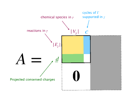
Figure 3: Structure of the A-matrix. The numbers $c$ and $\underline{d}$ are given by $c=|(\ker S)_{{\rm supp}\,\gamma}|$ and $\underline{d}=|P^{0}_{\gamma}(\mathop{{\rm coker}}S)|$.

The index $\lambda(\gamma)$ measures how far the black rectangle on the upper-left corner is from a square matrix. The numbers $c$ and $\underline{d}$ in Fig. 3 are given by $c=|(\ker S)_{{\rm supp}\,\gamma}|$ and $\underline{d}=|P^{0}_{\gamma}(\mathop{{\rm coker}}S)|$, which appear in Eq. (72). Because of the assumption of regularity, we have $\det A\neq 0$, and the black rectangle on the upper-left corner should be vertically long (if it is horizontally long, the determinant vanishes), which is equivalent to the condition $\lambda(\gamma)\geq 0$.

When $\lambda(\gamma)=0$, the black box in the upper-left corner is a square matrix. Then, $A^{-1}$ inherits the same structure,

$$A^{-1}=\begin{pmatrix}*&*\\ \bm{0}&*\end{pmatrix}.$$ (77)

Namely, if we denote the generic index of $(A^{-1})$ as $\mu,\nu,\cdots$ and write the index inside and outside $\gamma$ as $\mu^{\star}$ and $\mu^{\prime}$, respectively, we have $(A^{-1})_{\mu^{\prime}\nu^{\star}}=0$. Because of this structure,

$$\partial_{A^{\star}}x_{i^{\prime}}\propto(A^{-1})_{i^{\prime}A^{\star}}=0,$$ (78)

which means that the concentrations out of $\gamma$ do not depend on the parameter $k_{B}$ inside $\gamma$. Consequently, we have

$$\partial_{A^{\star}}r_{A^{\prime}}\propto\sum_{i^{\prime}}\partial_{i^{\prime}}r_{A^{\prime}}\partial_{A^{\star}}x_{i^{\prime}}=0,$$ (79)

where we used the fact that $r_{A^{\prime}}$ only depends on the concentrations outside $\gamma$ because of the output-completeness. The same is true for the perturbation of the conserved charge,

$$\partial_{{\bar{\alpha}}^{\star}}x_{i^{\prime}}\propto(A^{-1})_{i^{\prime}{\bar{\alpha}}^{\star}}=0,\quad\partial_{{\bar{\alpha}}^{\star}}r_{A^{\prime}}\propto\sum_{i^{\prime}}\partial_{i^{\prime}}r_{A^{\prime}}\partial_{{\bar{\alpha}}^{\star}}x_{i^{\prime}}=0.$$ (80)

∎

III.3 Submodularity of the influence index

The influence index $\lambda(\gamma)$ can be regarded as a function over subnetworks. We here show that the influence index satisfies an inequality. As a corollary, we show that the buffering structures are closed under union and intersection. This fact is useful in enumerating buffering structures in large reaction networks.

We first note that:

• Given output-complete subnetworks $\gamma_{1},\gamma_{2}\subset\Gamma$, the union and intersection, $\gamma_{1}\cup\gamma_{2}$ and $\gamma_{1}\cap\gamma_{2}$, are also output-complete. This follows from the definition of output-completeness.

• A function $f(\gamma)$ over a set is called submodular, when it satisfies

  $$f(\gamma_{1}\cup\gamma_{2})\leq f(\gamma_{1})+f(\gamma_{2})-f(\gamma_{1}\cap\gamma_{2}).$$ (81)

  When $\leq$ is replaced with $\geq$, the function satisfying the replaced equation is called supermodular.

Theorem 2.

Let $\gamma_{1},\gamma_{2}\subset\Gamma$ be output-complete subnetworks. The influence index satisfies

$$\lambda(\gamma_{1}\cup\gamma_{2})\leq\lambda(\gamma_{1})+\lambda(\gamma_{2})-\lambda(\gamma_{1}\cap\gamma_{2}).$$ (82)

Namely, $\lambda(\gamma)$ is a submodular function over output-complete subnetworks.

Proof.

We show that

$$\lambda(\gamma)=-|V_{\gamma}|+|E_{\gamma}|-|(\ker S)_{{\rm supp}\,\gamma}|+|P^{0}_{\gamma}(\mathop{{\rm coker}}S)|$$ (83)

is submodular. Recall that $\chi(\gamma)=|V_{\gamma}|-|E_{\gamma}|=|H_{0}(\gamma)|-|H_{1}(\gamma)|$ is the Euler number for subnetwork $\gamma=(V_{\gamma},E_{\gamma})$. We note that $\chi(\gamma)$ is a modular function, meaning that it satisfies

$$\chi(\gamma_{1}\cup\gamma_{2})=\chi(\gamma_{1})+\chi(\gamma_{2})-\chi(\gamma_{1}\cap\gamma_{2}),$$ (84)

which is derived from the Mayer-Vietoris exact sequence (56). Thus, it suffices to show that the last two terms on the right-hand side (RHS) of Eq. (83) are submodular. In fact, we show that each of them is submodular.

Let us first look at $|P^{0}_{\gamma}(\mathop{{\rm coker}}S)|$. If denote $W\coloneqq\mathop{{\rm coker}}S$, the submodularity of $|P^{0}_{\gamma}(\mathop{{\rm coker}}S)|$ reads

$$|P^{0}_{\gamma_{1}\cup\gamma_{2}}W|\leq|P^{0}_{\gamma_{1}}W|+|P^{0}_{\gamma_{2}}W|-|P^{0}_{\gamma_{1}\cap\gamma_{2}}W|.$$ (85)

We prove this equation just after this proof. Thus, we have shown the submodularity of $|P^{0}_{\gamma}(\mathop{{\rm coker}}S)|$.

Next, we show that $|(\ker S)_{{\rm supp}\,\gamma}|$ is supermodular. Consider the following vector space,

$$Z\coloneqq(\ker S)_{{\rm supp}\,\gamma_{1}}+(\ker S)_{{\rm supp}\,\gamma_{2}}.$$ (86)

Its dimension is given by

$$\begin{split}|Z|&=|(\ker S)_{{\rm supp}\,\gamma_{1}}|+|(\ker S)_{{\rm supp}\,\gamma_{2}}|-|(\ker S)_{{\rm supp}\,\gamma_{1}}\cap(\ker S)_{{\rm supp}\,\gamma_{2}}|\\ &=|(\ker S)_{{\rm supp}\,\gamma_{1}}|+|(\ker S)_{{\rm supp}\,\gamma_{2}}|-|(\ker S)_{{\rm supp}\,\gamma_{1}\cap\gamma_{2}}|.\end{split}$$ (87)

Since any element of $Z$ is supported in $\gamma_{1}\cup\gamma_{2}$, we have $(\ker S)_{{\rm supp}\,\gamma_{1}\cup\gamma_{2}}\supset Z$, which implies $|(\ker S)_{{\rm supp}\,\gamma_{1}\cup\gamma_{2}}|\geq|Z|$. Thus, we have shown that $|(\ker S)_{{\rm supp}\,\gamma}|$ is a supermodular function, and $-|(\ker S)_{{\rm supp}\,\gamma}|$ is submodular.

Therefore, $|P^{0}_{\gamma}(\mathop{{\rm coker}}S)|$ and $-|(\ker S)_{{\rm supp}\,\gamma}|$ are both submodular function, and we obtain the claim. ∎

Proof of Eq. (85). Let us pick a basis of the space $W$ as $\{\bm{w}_{1},\cdots,\bm{w}_{n}\}$ and we denote the basis as a matrix, $w_{ij}$. The set of possible row and column indices are denoted as $V$ and $N$, respectively. For a subset of indices $v\subset V$, we denote the corresponding submatrix of $w_{ij}$ as $w[v,N]$. With this notation, the dimension of a projected subspace of $W$ is written as $|P^{0}_{\gamma}W|={\rm rank\,}w[v_{\gamma},N]$ for a subnetwork $\gamma=(v_{\gamma},e_{\gamma})$.

Let us pick two subnetworks $\gamma_{1}$ and $\gamma_{2}$, and denote the sets of chemical species by $v_{1}$ and $v_{2}$, respectively. We consider the submatrix $w[v_{1}\cap v_{2},N]$. We can pick a row basis as $\{\bm{a}_{i}^{T}\,|\,i\in\alpha_{1\cap 2}\}$, where $\alpha_{1\cap 2}\subset v_{1}\cap v_{2}$. Here, $|\alpha_{1\cap 2}|={\rm rank\,}w[v_{1}\cap v_{2},N]$. We can form a row basis of $w[v_{1},N]$ by adding row vectors from $w[v_{1}\setminus v_{2},N]$ to $\alpha_{1\cap 2}$. Let $\alpha_{1}$ be the picked indices, then

$$|\alpha_{1\cap 2}|+|\alpha_{1}|={\rm rank\,}w[v_{1},N].$$ (88)

We can further pick row vectors from $w[v_{2}\setminus v_{1},N]$ and form a basis of $w[v_{1}\cup v_{2},N]$. Let us denote the added indices as $\alpha_{2}$, then

$$|\alpha_{1\cap 2}|+|\alpha_{1}|+|\alpha_{2}|={\rm rank\,}w[v_{1}\cup v_{2},N].$$ (89)

Since the vectors specified by the indices $\alpha_{1\cap 2}\cup\alpha_{2}$ are linearly independent and $\alpha_{1\cap 2}\cup\alpha_{2}\subset v_{2}$, we have $|\alpha_{1\cap 2}|+|\alpha_{2}|\leq{\rm rank\,}w[v_{2},N]$. This can be written as

$${\rm rank\,}w[v_{1}\cup v_{2},N]\leq{\rm rank\,}w[v_{1},N]+{\rm rank\,}w[v_{2},N]-{\rm rank\,}w[v_{1}\cap v_{2},N].$$ (90)

This is equivalent to Eq. (85).

$\Box$

Corollary 1.

Let $\Gamma$ be a regular chemical reaction network. The union and the intersection of two buffering structures inside $\Gamma$ are also buffering structures.

Proof.

Suppose $\gamma_{1}$ and $\gamma_{2}$ are buffering structures inside $\Gamma$. Then $\lambda(\gamma_{1})=\lambda(\gamma_{2})=0$. From the submodularity of the influence index, we have

$$\lambda(\gamma_{1}\cup\gamma_{2})+\lambda(\gamma_{1}\cap\gamma_{2})\leq 0.$$ (91)

Since influence indices are nonnegative for a regular chemical reaction network, we have $\lambda(\gamma_{1}\cup\gamma_{2})=\lambda(\gamma_{1}\cap\gamma_{2})=0$. Thus, we obtain the claim. ∎

IV Reduction of chemical reaction networks

Generically, a reduction is a process to reduce the number of degrees of freedom while keeping some features of the original system. Let us here introduce a reduction method which consists of the following two steps,

• Identify a subnetwork to be reduced.

• Perform the reduction for given a subnetwork.

As a result, we obtain a new reaction network with fewer chemical species and reactions,

$$\Gamma\longrightarrow\Gamma^{\prime}.$$ (92)

The reduced network is characterized by a new stoichiometric matrix,

$$S\longrightarrow S^{\prime}.$$ (93)

Crucial points are, how to identify a subnetwork to be eliminated, and how to obtain the new stoichiometric matrix $S^{\prime}$, which determines the structure of the reduced network. In this section, we mainly discuss step (2). We will discuss more on the choice of a subnetwork in Sec. (V).

IV.1 Reduction procedure

Let us here illustrate a method of reduction based on the network topology. We denote the whole reaction network by $\Gamma=(V,E)$, where $V$ and $E$ are the sets of chemical species and reactions, respectively. We choose a subnetwork $\gamma=(V_{\gamma},E_{\gamma})$, where $V_{\gamma}\subset V$ and $E_{\gamma}\subset E$, and eliminate the degrees of freedom inside $\gamma$. We refer to the chemical species and reactions inside $\gamma$ as internal, and those in $\Gamma\setminus\gamma$ as boundary. For the given subnetwork $\gamma$, we separate the chemical concentrations and reaction rates as

$$\bm{x}=\begin{pmatrix}\bm{x}_{1}\\ \bm{x}_{2}\end{pmatrix},\quad\bm{r}=\begin{pmatrix}\bm{r}_{1}\\ \bm{r}_{2}\end{pmatrix},$$ (94)

where $1$ and $2$ correspond to internal and boundary degrees of freedom, respectively. Accordingly, the stoichiometric matrix $S$ can be partitioned as

$$S=\begin{pmatrix}S_{11}&S_{12}\\ S_{21}&S_{22}\end{pmatrix}.$$ (95)

Note that the submatrix $S_{11}$ is the same matrix as $S_{\gamma}$ that appeared in Sec. II.3. Hereafter we use $S_{11}$ for notational convenience. With the separation of internal and boundary degrees of freedom, the rate equations of the whole reaction system is written as

$$\frac{d}{dt}\begin{pmatrix}\bm{x}_{1}\\ \bm{x}_{2}\end{pmatrix}=\begin{pmatrix}S_{11}&S_{12}\\ S_{21}&S_{22}\end{pmatrix}\begin{pmatrix}\bm{r}_{1}\\ \bm{r}_{2}\end{pmatrix}=\begin{pmatrix}S_{11}\bm{r}_{1}+S_{12}\bm{r}_{2}\\ S_{21}\bm{r}_{1}+S_{22}\bm{r}_{2}\end{pmatrix}.$$ (96)

While the internal reaction rates $\bm{r}_{1}=\bm{r}_{1}(\bm{x}_{1},\bm{x}_{2})$ in general depend on both of the internal and boundary chemical concentrations, when $\gamma$ is chosen to be output-complete, the boundary reaction rates $\bm{r}_{2}=\bm{r}_{2}(\bm{x}_{2})$ do not depend on the internal chemical concentrations $\bm{x}_{1}$. The first equation of Eq. (96) can be solved for $\bm{r}_{1}$ as

$$\bm{r}_{1}=S_{11}^{+}\frac{d}{dt}\bm{x}_{1}-S_{11}^{+}S_{12}\bm{r}_{2}+\bm{c}_{11},$$ (97)

where $S_{11}^{+}$ is the Moore-Penrose inverse of $S_{11}$, and $\bm{c}_{11}\in\ker S_{11}$. Substituting this to the second equation of Eq. (96), we get

$$\frac{d}{dt}\left({\bm{x}}_{2}-S_{21}S^{+}_{11}{\bm{x}}_{1}\right)=(S_{22}-S_{21}S_{11}^{+}S_{12})\bm{r}_{2}+S_{21}\bm{c}_{11}.$$ (98)

When the following condition is satisfied,

$$\ker S_{11}\subset\ker S_{21},$$ (99)

$S_{21}\bm{c}_{11}=\bm{0}$ and the second term of the RHS of Eq. (98) vanishes. Then, the rate equation is written as

$$\frac{d}{dt}\left({\bm{x}}_{2}-S_{21}S^{+}_{11}{\bm{x}}_{1}\right)=S^{\prime}\bm{r}_{2},$$ (100)

where $S^{\prime}$ is the generalized Schur complement,

$$S^{\prime}=S/S_{11}\coloneqq S_{22}-S_{21}S_{11}^{+}S_{12}.$$ (101)

As long as steady states are concerned, the subnetwork $(\bm{x}_{2},\bm{r}_{2})$ satisfies the rate equation whose stoichiometric matrix is $S^{\prime}$. This motivates us to consider the subnetwork $(\bm{x}_{2},\bm{r}_{2})$ whose rate equation is given by

$$\frac{d}{dt}{\bm{x}}_{2}=S^{\prime}\bm{r}_{2}(\bm{x}_{2}).$$ (102)

Based on the considerations above, we define the reduction of a reaction system in the following way:

Definition 6 (Reduction).

Let $\Gamma=(V,E)$ be a chemical reaction network with stoichiometric matrix $S$ and $\gamma=(V_{\gamma},E_{\gamma})$ be an output-complete subnetwork whose stoichiometric matrix is denoted by $S_{11}$. We define a reduced network $\Gamma^{\prime}=(V\setminus V_{\gamma},E\setminus E_{\gamma})$ obtained by eliminating $\gamma$ from $\Gamma$, by a stoichiometric matrix $S^{\prime}$ given by the generalized Schur complement (101). We denote the resultant reaction network by $\Gamma^{\prime}=\Gamma/\gamma$. Accordingly, the chemical concentrations and reaction rates of the reduced system $(\bm{x}^{\prime},\bm{r}^{\prime})$ are obtained from the original ones $(\bm{x},\bm{r})$ as

$$\bm{x}=\begin{pmatrix}\bm{x}_{1}\\ \bm{x}_{2}\end{pmatrix} \longrightarrow\bm{x}^{\prime}=\bm{x}_{2},$$ (103)

$$\bm{r}(\bm{x})=\begin{pmatrix}\bm{r}_{1}(\bm{x}_{1},\bm{x}_{2})\\ \bm{r}_{2}(\bm{x}_{2})\end{pmatrix} \longrightarrow\bm{r}^{\prime}(\bm{x}^{\prime})=\bm{r}_{2}(\bm{x}_{2}),$$ (104)

and the rate equation of the reduced system is given by

$$\frac{d}{dt}{\bm{x}}^{\prime}=S^{\prime}\bm{r}^{\prime}(\bm{x}^{\prime}).$$ (105)

Remark 9.

The structure of the reduced network is determined by the generalized Schur complement (101) of the stoichiometric matrix. The second term in Eq. (101) represents the rewiring of the network associated with the elimination of $\gamma$.

Remark 10.

The reduced system can be always defined if $\gamma$ is output-complete; otherwise, the reduction is ill-defined since the reduced system would depend on $\bm{x}_{1}$ through $\bm{r}_{2}$. We emphasize that the output-completeness is a topological condition determined by the stoichiometry and the details of the reactions, namely the kinetics, are irrelevant. Thus, the reduction is applicable to any kind of kinetics. How the reduced system is related to the original system depends on further nature of $\gamma$. In the following sections, we will discuss more on the features of the subnetworks that behave nicely under reductions. In Sec. V.3, we prove that, when $\gamma$ has a vanishing influence index (see Sec. III), which is determined by the network topology, the steady state of the reduced system is assured to be the same as the steady state of the original system.

Remark 11.

In Sec. IV.3, we show that the reduction we introduced here can be regarded as a morphism of reaction networks that ‘shrinks’ a subnetwork to a point, followed by the removal of degenerate (chemically meaningless) reactions.

Remark 12.

We note that the elements of the matrix $S^{\prime}$ are rational, since the Moore-Penrose inverse of an integral matrix is rational [48]. The matrix $S^{\prime}$ can be always transformed into an integral matrix by columnwise rescaling of $S^{\prime}$ together with the rescaling of reaction rates.

Remark 13.

The stoichiometric matrix given by the generalized Schur complement has appeared previously in flux balance analysis [49, 50]. The current method is different from the ones discussed for reaction networks with the mass-action kinetics in detailed balanced [51] and complex balanced [52] situations, where the Schur complementation is performed for the weighted Laplacian similarly to the Kron reduction of electrical circuits [53, 54, 55]. In the current formulation, the Schur complementation is performed for the stoichiometric matrix.

IV.2 Simple examples of reduction

To illustrate the reduction procedure, here we discuss simple examples. In Sec. VI, we discuss the reduction of the metabolic pathway of E. coli as a more realistic example.

Example 5.

We consider a monomolecular reaction network that consists of $(V,E)=(\{v_{1},v_{2}\},\{e_{1},e_{2},e_{2}\})$. We take a subnetwork $\gamma=(\{v_{1}\},\{e_{2}\})$ to be reduced. Under the reduction, the stoichiometric matrix changes as

(106)

where we have brought the reduced part to the upper-left part. The reduction looks like

(107)

The original rate equation is

$$\frac{d}{dt}\begin{pmatrix}x_{1}\\ x_{2}\end{pmatrix}=\begin{pmatrix}-1&1&0\\ 1&0&-1\\ \end{pmatrix}\begin{pmatrix}r_{2}(x_{1})\\ r_{1}\\ r_{3}(x_{2})\end{pmatrix},$$ (108)

where $x_{1}=x(v_{1})$, $r_{2}=r(e_{2})$ and so on. If we eliminate $r_{2}(x_{1})$,

$$\frac{d}{dt}\left(x_{2}+x_{1}\right)=\begin{pmatrix}1&-1\end{pmatrix}\begin{pmatrix}r_{1}\\ r_{3}(x_{2})\end{pmatrix}.$$ (109)

The reduced equation of motion is obtained by replacing $x_{2}+x_{1}$ with $x_{2}$ on the left-hand side.

To compute the steady-state solutions, let us for example employ the mass-action kinetics,

$$\begin{pmatrix}r_{2}(x_{1})\\ r_{1}\\ r_{3}(x_{2})\\ \end{pmatrix}=\begin{pmatrix}k_{2}x_{1}\\ k_{1}\\ k_{3}x_{2}\\ \end{pmatrix}.$$ (110)

The steady-state reaction rates and concentrations are given by

$$\begin{pmatrix}\bar{r}_{2}\\ \bar{r}_{1}\\ \bar{r}_{3}\\ \end{pmatrix}=k_{1}\begin{pmatrix}1\\ 1\\ 1\end{pmatrix},\quad\begin{pmatrix}\bar{x}_{1}\\ \bar{x}_{2}\end{pmatrix}=\begin{pmatrix}k_{1}/k_{2}\\ k_{1}/k_{3}\end{pmatrix}.$$ (111)

The steady-state solutions of the reduced system are

$$\begin{pmatrix}\bar{r}_{1}\\ \bar{r}_{3}\end{pmatrix}=k_{1}\begin{pmatrix}1\\ 1\end{pmatrix},\quad\bar{x}_{2}=\frac{k_{1}}{k_{3}}.$$ (112)

Note that this solution of the reduced system is exactly the same as the solution (111) of the original system for the boundary concentrations and rates. Indeed, this is a special property of buffering structures. In this example, the subnetwork has a vanishing influence index, $\lambda(\gamma)=-1+1-0+0=0$, and hence is a buffering structure. Generically, when the reduced subnetwork is a buffering structure, the steady-state solution of the reduced system is the same as the original system, and this is the content of Theorem 201. Although we used the mass-action kinetics in this example, the theorem applies to any kind of kinetics. We give a proof of the theorem in Sec. V.3.

Example 6.

$(V,E)=(\{v_{1},v_{2},v_{3}\},\{e_{1},e_{2},e_{3}\})$. The stoichiometric matrices of the original and reduced system are given by

where we reduced the subnetwork $\gamma=(\{v_{1}\},\{e_{1}\})$. The reduction is visually expressed as

(113)

Suppose that we take the mass-action kinetics,

$$\begin{pmatrix}r_{1}(x_{1})\\ r_{2}(x_{2})\\ r_{3}(x_{3})\\ \end{pmatrix}=\begin{pmatrix}k_{1}x_{1}\\ k_{2}x_{2}\\ k_{3}x_{3}\\ \end{pmatrix}.$$ (114)

The system has one conserved charge and we specify the value as $\ell=x_{1}+x_{2}+x_{3}.$ The steady-state reaction rates of the original system are

$$\begin{pmatrix}\bar{r}_{1}\\ \bar{r}_{2}\\ \bar{r}_{3}\end{pmatrix}=\ell K\begin{pmatrix}1\\ 1\\ 1\end{pmatrix},$$ (115)

where $K$ is defined by $\frac{1}{K}\coloneqq\frac{1}{k_{1}}+\frac{1}{k_{2}}+\frac{1}{k_{3}}.$ In the reduced system, $\ell^{\prime}=x_{2}+x_{3}$ is a conserved charge. The steady-state rates in the reduced system are

$$\begin{pmatrix}\bar{r}_{2}\\ \bar{r}_{3}\end{pmatrix}=\ell^{\prime}K^{\prime}\begin{pmatrix}1\\ 1\end{pmatrix},$$ (116)

where $\frac{1}{K^{\prime}}\coloneqq\frac{1}{k_{2}}+\frac{1}{k_{3}}.$ Note that, if we want to have the same steady-state in the reduced system as the one in the original system, we have to choose the parameters so that $\ell K=\ell^{\prime}K^{\prime}$. This is in contrast to Example 5, where no fine-tuning of the parameters is needed. The difference is attributed to the fact that the subnetwork $\gamma$ is not a buffering structure and the index is nonzero, $\lambda(\gamma)=-1+1-0+1=1$.

Example 7.

$(V,E)=(\{v_{1},v_{2},v_{3},v_{4}\},\{e_{1},e_{2},e_{3},e_{4},e_{5},e_{6}\})$. The stoichiometric matrix changes under reduction as

(117)

where we chose the subnetwork $\gamma=(\{v_{1},v_{2}\},\{e_{2},e_{3}\})$ to be reduced. The reduction is visually expressed as

(118)

The subnetwork is a buffering structure, $\lambda(\gamma)=-2+2-0+0=0$.

Example 8.

$(V,E)=(\{v_{1},\ldots,v_{9}\},\{e_{1},\ldots,e_{13}\})$ with the following stoichiometric matrix,

.

We choose the subnetwork $\gamma=(\{v_{3},v_{4},v_{5},v_{7},v_{8}\},\{e_{5},e_{6},e_{7},e_{8},e_{9},e_{11},e_{12}\})$ to be reduced. The reduced subnetwork is given by

.

The subnetwork $\gamma$ is a buffering structure: $\lambda(\gamma)=-5+7-2+0=0$. The reduction is visually expressed as

(119)

We note that, under the reduction, the stoichiometries for reactions $e_{3},\ e_{4},\ e_{10}$ are changed from the original ones. In particular, $e_{10}$, which is originally monomolecular, becomes non-monomolecular, $2v_{6}\rightarrow v_{9}$. To reproduce steady states of the original system, the rate $r_{10}$ is required to be the same as before the reduction; for example, in the mass-action kinetics, $r_{10}$ is given by $r_{10}(x_{6})=k_{10}x_{6}$ rather than by $r_{10}(x_{6})=k_{10}x_{6}^{2}$, even after the reduction.

IV.3 Reduction as a morphism of chemical reaction networks

The structure of a reduced network is characterized by the generalized Schur complement (101). Here, let us show that this form arises if we consider a map between chemical reactions that shrink a subnetwork to a point. The morphisms of chemical reaction networks have been discussed, for example, in Ref. [56]. Let us prepare some terminologies.

Definition 7.

(Degenerate reactions) A reaction $e\in E$ is said to be degenerate in stoichiometry if $s(e)(v_{i})=t(e)(v_{i})$ for any $v_{i}\in V$.

A degenerate reaction is a trivial reaction since it does not change anything, and the removal of degenerate reactions does not affect the chemical properties of the reaction network. A degenerate reaction is represented as a $0-$column in the stoichiometric matrix.

Let us slightly extend the definition of CRNs for technical reasons.

Definition 8 (Generalized CRNs).

A generalized chemical reaction network $\Gamma$ is a quadruple $\Gamma=(V,E,s,t)$, where $V$ is a set of chemical species, $E$ is a set of chemical reactions, and $s$ and $t$ are source and target functions,

$$s:E\to{\mathbb{R}}^{V},\quad t:E\to{\mathbb{R}}^{V}.$$ (120)

Compared with the previous definition of a CRN, $\mathbb{N}$ is replaced with real numbers, $\mathbb{R}$. We also call an element of ${\mathbb{R}}^{V}$ as a chemical complex. In the remainder of this paper, we will mean a generalized CRN when we write a CRN. This extension is needed because the reductions we consider do not necessarily preserve the integrality of the source and target functions. However, we note that the integrality can be always recovered by reactionwise rescaling, if the original $s$ and $t$ functions are valued in integers.

Definition 9 (CRN morphisms).

A CRN morphism $\varphi$ from $\Gamma=(V,E,s,t)$ to $\Gamma^{\prime}=(V^{\prime},E^{\prime},s^{\prime},t^{\prime})$ is a pair of maps, $(\varphi_{0},\varphi_{1})$, where

$$\varphi_{0} : {\mathbb{R}}^{V}\to{\mathbb{R}}^{V^{\prime}},$$ (121)

$$\varphi_{1} : E\to E^{\prime},$$ (122)

which we call a chemical complex map and a reaction map, respectively, such that the following diagrams commute,

(123)

We introduce the matrix representation of a chemical complex map and a reaction map,

$$\varphi_{0}(v_{i}) =\sum_{i^{\prime}}(\varphi_{0})_{ii^{\prime}}\,v_{i^{\prime}},$$ (124)

$$\varphi_{1}(e_{A}) =\sum_{A^{\prime}}(\varphi_{1})_{AA^{\prime}}\,e_{A^{\prime}}.$$ (125)

On the spaces of chains, a CRN morphism induces the following commutative diagram,

(126)

where $\partial^{\prime}_{1}$ is the boundary operator on $C_{1}(\Gamma^{\prime})$. Namely,

$$\varphi_{0}\circ\partial_{1}=\partial^{\prime}_{1}\circ\varphi_{1}.$$ (127)

In terms of the matrix components,

$$\sum_{i}S_{iA}\,(\varphi_{0})_{ii^{\prime}}=\sum_{A^{\prime}}(\varphi_{1})_{AA^{\prime}}\,S^{\prime}_{i^{\prime}A^{\prime}}.$$ (128)

We write this relation in the matrix form,

$$\varphi_{0}^{T}S=S^{\prime}\varphi_{1}^{T}.$$ (129)

Now we are ready to discuss a morphism that corresponds to the reduction:

Definition 10 (Reduction morphisms).

We define a reduction morphism from $\Gamma$ to $\Gamma^{\prime}$, associated with a subnetwork $\gamma\subset\Gamma$, as a CRN morphism satisfying the following properties:

1. The chemical complexes and reactions in $\Gamma\setminus\gamma$ are unchanged.

2. All the chemical complexes in $\gamma$ are collapsed into one chemical complex $\bar{c}$ in $\Gamma\setminus\gamma$, in such a way that image of all the reactions in $\gamma$ are degenerate in stoichiometry.

Let us here show that a reduction morphism gives rise to the reduced stoichiometric matrix given by the generalized Schur complement (101). We consider the matrix representation of a reduction morphism. From property 2 of reduction morphisms, the chemical complex map and the reaction map are both identity on $v_{i}\in V_{\Gamma\setminus\gamma}$ and $e_{A}\in E_{\Gamma\setminus\gamma}$,

$$\varphi_{0}|_{\Gamma\setminus\gamma}=\bm{1},\quad\varphi_{1}|_{\Gamma\setminus\gamma}=\bm{1}.$$ (130)

Furthermore, we can always set $\varphi_{1}|_{\gamma}=\bm{1}$ without affecting the chemical properties, since degenerate reactions do nothing chemically. By arranging the rows and columns, the species and reaction maps of a reduction morphism can be written in the following form,

$$\varphi_{0}=\begin{pmatrix}F^{T}\\ \bm{1}\end{pmatrix},\quad\varphi_{1}=\bm{1},$$ (131)

where $F$ is some matrix (see examples later in this section). The explicit form of $F$ does not matter here. By plugging Eq. (131) into the commutativity condition (129), we find that $S^{\prime}$ is written as

$$S^{\prime}=\begin{pmatrix}F&\bm{1}\end{pmatrix}\begin{pmatrix}S_{11}&S_{12}\\ S_{21}&S_{22}\end{pmatrix}=\begin{pmatrix}FS_{11}+S_{21}&\,\,FS_{12}+S_{22}\end{pmatrix}.$$ (133)

From the condition that the image of the reactions in $\gamma$ under a reduction morphism is degenerate reactions, we have

$$FS_{11}+S_{21}=\bm{0}.$$ (134)

This condition implies

$$\ker S_{11}\subset\ker S_{21}.$$ (135)

This is because, if $\bm{c}\in\ker S_{11}$, Eq. (134) implies $S_{21}\bm{c}=\bm{0}$, we have Eq. (135). A generic solution to Eq. (134) for $F$ is written as

$$F=-S_{21}S_{11}^{+}+D,$$ (136)

where $D$ is a matrix satisfying $DS_{11}=0$. The stoichiometric matrix $S^{\prime}$ can be now written as

$$S^{\prime}=\begin{pmatrix}\bm{0}&\,\,S_{22}-S_{21}S_{11}^{+}S_{12}+DS_{12}\end{pmatrix}.$$ (137)

The term $DS_{12}$ vanishes if and only if

$$\mathop{{\rm coker}}S_{11}\subset\mathop{{\rm coker}}S_{12}.$$ (138)

Note that the combination $S_{21}S_{11}^{+}S_{12}$ does not depend on the choice of the pseudo-inverse, as long as Eqs. (135) and (138) are satisfied. After removing degenerate reactions from Eq. (137), which does not change the chemical property of the system, we arrive at the generalized Schur complement (101) that we introduced earlier. In this way, a CRN morphism that shrinks a subnetwork gives rise to the reduced stoichiometric matrix given by the Schur complement.

What we have just shown can be summarized as the following statement:

Theorem 3.

Under a reduction morphism associated with $\gamma\subset\Gamma$, the stoichiometric matrix of $\Gamma^{\prime}$ can be written uniquely (up to the changes of rows and columns) in the form

$$S^{\prime}=\begin{pmatrix}\bm{0}&\,\,S_{22}-S_{21}S_{11}^{+}S_{12}\end{pmatrix},$$ (139)

if and only if the following conditions are satisfied for the subnetwork $\gamma$,

$$\ker S_{11}\subset\ker S_{21},\quad\mathop{{\rm coker}}S_{11}\subset\mathop{{\rm coker}}S_{12}.$$ (140)

Conversely, for a given output-complete subnetwork such that Eq. (140) is satisfied, we can construct the following reduction map by

$$\varphi_{0}=\begin{pmatrix}(-S_{21}S^{+}_{11}+D)^{T}\\ \bm{1}\end{pmatrix},\quad\varphi_{1}=\bm{1},$$ (141)

where $D$ is a matrix satisfying $DS_{11}=\bm{0}$. The commutativity condition reads

$$S^{\prime}=\begin{pmatrix}S_{21}(\bm{1}-S_{11}^{+}S_{11})&\,\,S_{22}-S_{21}S^{+}_{11}S_{12}+DS_{12}\end{pmatrix}.$$ (142)

Since $(\bm{1}-S_{11}^{+}S_{11})$ is a projection matrix to $\ker S_{11}$ and we have $\ker S_{11}\subset\ker S_{21}$ by assumption, the matrix $S_{21}(\bm{1}-S_{11}^{+}S_{11})$ is a zero matrix. Furthermore, $DS_{12}=\bm{0}$ by the assumption $\mathop{{\rm coker}}S_{11}\subset\mathop{{\rm coker}}S_{12}$. Thus, we arrive at the reduced stoichiometric matrix of the form (139).

Below, let us illustrate reduction morphisms in simple examples.

Example 9.

Let us consider the following closed directed graph. We consider the morphism, which can be pictorially represented as

(143)

The reduction shrinks the vertices in $\gamma$ to a single complex, $\bar{c}=v_{3}^{\prime}$. The species and reactions are mapped as

$$\varphi_{0}(v_{1}) =v_{1}^{\prime},\quad\varphi_{0}(v_{2})=v_{3}^{\prime},\quad\varphi_{0}(v_{3})=v_{3}^{\prime},\quad\varphi_{0}(v_{4})=v_{4}^{\prime},$$ (144)

$$\varphi_{1}(e_{1}) =e_{1}^{\prime},\quad\varphi_{1}(e_{2})=e_{2}^{\prime},\quad\varphi_{1}(e_{3})=e_{3}^{\prime}.$$ (145)

In the matrix form,

$$\varphi_{0}=\blockarray{cccc}&\\ \block{c(ccc)}{\color[rgb]{0.9140625,0.078125,0.13671875}v_{2}}\quad\,010\\ v_{1}\quad\,100\\ v_{3}\quad\,010\\ v_{4}\quad\,001\\ {v_{1}^{\prime}}v_{3}^{\prime}v_{4}^{\prime}\quad,\quad\varphi_{1}=\bm{1}_{3}.$$ (146)

Using the consistency condition (129), the stoichiometric matrix of $\Gamma^{\prime}$ can be written as

$$S^{\prime}=\begin{pmatrix}0&1&0&0\\ 1&0&1&0\\ 0&0&0&1\end{pmatrix}\begin{pmatrix}-1&1&0\\ 0&-1&0\\ 1&0&-1\\ 0&0&1\end{pmatrix}\bm{1}_{3}=\blockarray{cccc}&\\ \block{c(ccc)}v_{1}^{\prime}\quad\,0-10\\ v_{3}^{\prime}\quad\,01-1\\ v_{4}^{\prime}\quad\,001\\ e_{2}^{\prime}e_{1}^{\prime}e_{3}^{\prime}\,\,\,\,.$$ (147)

This is indeed of the form (139).

Example 10.

$\Gamma=(\{v_{1},v_{2},v_{3}\},\{e_{1},e_{2}\})$. We consider the reduction of $\gamma=(\{v_{1}\},\{e_{1}\})$. The corresponding reduction morphism is visualized as

(148)

The chemical complex map and the reaction map are given by

$$\varphi_{0}(v_{1}) =v^{\prime}_{2}+v^{\prime}_{3},\quad\varphi_{0}(v_{2})=v^{\prime}_{2},\quad\varphi_{0}(v_{3})=v^{\prime}_{3},$$ (149)

$$\varphi_{1}(e_{1}) =e_{1}^{\prime},\quad\varphi_{1}(e_{2})=e_{2}^{\prime}.$$ (150)

The action $\varphi_{0}(v_{1})$ is determined so that the image of $e_{1}$ be degenerate in stoichiometry. The image of $e_{1}$ is the following degenerate reaction,

$$e_{1}^{\prime}:v^{\prime}_{2}+v^{\prime}_{3}\to v^{\prime}_{2}+v^{\prime}_{3}.$$ (151)

In the matrix form,

$$\varphi_{0}=\blockarray{ccc}&\\ \block{c(cc)}{\color[rgb]{0.9140625,0.078125,0.13671875}v_{1}}\quad\,11\\ v_{2}\quad\,10\\ v_{3}\quad\,01\\ {v_{2}^{\prime}}v_{3}^{\prime}\,\,\,,\quad\varphi_{1}=\bm{1}_{2}.$$ (152)

The stoichiometric matrix of $\Gamma^{\prime}$ is written as

$$S^{\prime}=\begin{pmatrix}1&1&0\\ 1&0&1\end{pmatrix}\begin{pmatrix}-1&0\\ 1&-1\\ 1&1\end{pmatrix}=\begin{pmatrix}0&-1\\ 0&1\end{pmatrix}.$$ (153)

V Reduction and buffering structures

We here explore the close connection between the structural sensitivity analysis and the reduction method we introduced in the previous section. The structural sensitivity analysis works as a guide to identify ’unimportant’ subnetworks. In this section, we present a key result of this paper: we show that, when a subnetwork is a buffering structure, the reduced network has exactly the same steady-state solution as the original reaction network. The proof will be completed in Sec. V.3.

The structure of this section is as follows: In Sec. V.1, we show that the influence index allows for a decomposition in terms of the numbers of cycles and conserved charges. In Sec. V.2, we construct a short exact sequence of the chain complexes for a subnetwork $\gamma\subset\Gamma$, under some conditions. This short exact sequence automatically derives a long exact sequence of homology groups. Using this exact sequence, we can describe the relationship among cycles and conserved charges of $\gamma$, $\Gamma$ and $\Gamma^{\prime}$. In Sec. V.3, we show the main result, that is, that the steady state of the reduced network is the same as the one of the original network, under some conditions. In the proof, the long exact sequence prepared in subsection B plays an important role. In Sec. V.4, we study the situation where we have nested subnetworks $\gamma^{\prime}\subset\gamma\subset\Gamma$. In this case, we have a subnetwork $\gamma/\gamma^{\prime}\subset\Gamma/\gamma^{\prime}$. We will show that the reduced network $\Gamma/\gamma$ is the same as $(\Gamma/\gamma^{\prime})/(\gamma/\gamma^{\prime})$. This ensures that the eventual network does not depend on the ordering of the reductions.

V.1 Decomposition of the influence index

As we detailed in Sec. II, steady-state properties are captured by cycles and conserved charges, which are the elements of homology groups. In this subsection, we study their meaning in more detail, and discuss the relation between the influence index $\lambda(\gamma)$ and cycles/conserved charges in $\gamma$, $\Gamma$, and $\Gamma^{\prime}$. We introduce a decomposition of the influence index in terms of the spaces of cycles/conserved charges of certain classes.

We first note that the index can be written as

$$\begin{split}\lambda(\gamma)&=-|V_{\gamma}|+|E_{\gamma}|-|(\ker S)_{{\rm supp}\,\gamma}|+|P^{0}_{\gamma}(\mathop{{\rm coker}}S)|\\ &=|\ker S_{11}|-|(\ker S)_{{\rm supp}\,\gamma}|+|P^{0}_{\gamma}(\mathop{{\rm coker}}S)|-|\mathop{{\rm coker}}S_{11}|,\end{split}$$ (154)

where we used Eq. (51). With the first two terms, we define

$$\widetilde{c}(\gamma)\coloneqq|\ker S_{11}|-|(\ker S)_{{\rm supp}\,\gamma}|.$$ (155)

The number $\widetilde{c}(\gamma)$ is a nonnegative integer, because there is an injective map from $(\ker S)_{{\rm supp}\,\gamma}$ to $\ker S_{11}$. Indeed, an element of $(\ker S)_{{\rm supp}\,\gamma}$ is written as $\bm{c}=\begin{pmatrix}\bm{c}_{1}\\ \bm{0}\end{pmatrix}$ satisfying the condition

$$\begin{pmatrix}S_{11}&S_{12}\\ S_{21}&S_{22}\end{pmatrix}\begin{pmatrix}\bm{c}_{1}\\ \bm{0}\end{pmatrix}=\begin{pmatrix}S_{11}\bm{c}_{1}\\ S_{21}\bm{c}_{1}\end{pmatrix}=\bm{0}.$$ (156)

Consider an injective map $\bm{c}\mapsto\bm{c}_{1}$. Equation (156) indicates that the image of this map is always included in $\ker S_{11}$,

$$(\ker S)_{{\rm supp}\,\gamma}\ni\bm{c}\mapsto\bm{c}_{1}\in\ker S_{11}.$$ (157)

Thus, we have $\widetilde{c}(\gamma)\geq 0$.

Now let us turn to the latter two terms in Eq. (154). Note that

$$|P^{0}_{\gamma}(\mathop{{\rm coker}}S)|=|\mathop{{\rm coker}}S|-|{\rm im}\,\bar{P}^{0}_{\gamma}\cap\mathop{{\rm coker}}S|,$$ (159)

where $\bar{P}^{0}_{\gamma}\coloneqq 1-P^{0}_{\gamma}$. The second term of the RHS of Eq. (159) is the number of the conserved charges of $\Gamma$ supported in $\Gamma\setminus\gamma$,

$$\bar{d}^{\prime}(\gamma)\coloneqq|{\rm im}\,\bar{P}^{0}_{\gamma}\cap\mathop{{\rm coker}}S|=|\bar{D}^{\prime}(\gamma)|,$$ (160)

where the space $\bar{D}^{\prime}(\gamma)$ is given by

$$\bar{D}^{\prime}(\gamma)\coloneqq\left\{\begin{pmatrix}\bm{d}_{1}\\ \bm{d}_{2}\end{pmatrix}\in\mathop{{\rm coker}}S\,\middle|\,\bm{d}_{1}=\bm{0}\right\}.$$ (161)

We divide the space $\mathop{{\rm coker}}S$ according to the following distinctions:

• Projection to $\gamma$ is also a conserved charge in $\gamma$.

• Projection to $\gamma$ is not a conserved charge in $\gamma$.

Correspondingly to the two distinctions above, we introduce the following spaces,

$$D(\gamma) \coloneqq X(\gamma)/\bar{D}^{\prime}(\gamma),$$ (162)

$$D^{\prime}(\gamma) \coloneqq\mathop{{\rm coker}}S/D(\gamma)\cong(\mathop{{\rm coker}}S)/X(\gamma)\oplus\bar{D}^{\prime}(\gamma),$$ (163)

where we defined

$$X(\gamma)\coloneqq\left\{\begin{pmatrix}\bm{d}_{1}\\ \bm{d}_{2}\end{pmatrix}\in\mathop{{\rm coker}}S\,\middle|\,\bm{d}_{1}\in\mathop{{\rm coker}}S_{11}\right\}.$$ (164)

Namely, we have the following decomposition of $\mathop{{\rm coker}}S$,

$$\mathop{{\rm coker}}S\cong D(\gamma)\oplus D^{\prime}(\gamma)\cong D(\gamma)\oplus(\mathop{{\rm coker}}S)/X(\gamma)\oplus\bar{D}^{\prime}(\gamma).$$ (165)

The dimension of $\mathop{{\rm coker}}S$ is written as

$$|\mathop{{\rm coker}}S|=d(\gamma)+d^{\prime}(\gamma),$$ (166)

where $d(\gamma)\coloneqq|D(\gamma)|$, and $d^{\prime}(\gamma)\coloneqq|D^{\prime}(\gamma)|$. We now have the expression

$$|P^{0}_{\gamma}(\mathop{{\rm coker}}S)|=d(\gamma)+d^{\prime}(\gamma)-\bar{d}^{\prime}(\gamma).$$ (167)

To rewrite $|\mathop{{\rm coker}}S_{11}|$, we introduce the following spaces,

$$D_{11}(\gamma) \coloneqq\left\{\bm{d}_{1}\in\mathop{{\rm coker}}S_{11}\,\middle|\,{}^{\exists}\bm{d}_{2}{\text{ such that }}\begin{pmatrix}\bm{d}_{1}\\ \bm{d}_{2}\end{pmatrix}\in\mathop{{\rm coker}}S\right\},$$ (168)

$$\widetilde{D}(\gamma) \coloneqq\mathop{{\rm coker}}S_{11}/D_{11}(\gamma).$$ (169)

The elements of $D_{11}(\gamma)$ are conserved charges in $\gamma$ that can be extended to a global conserved charge, while those in $\widetilde{D}(\gamma)$ are emergent conserved charges that are only conserved in the subnetwork $\gamma$.

Observe that $D(\gamma)\cong D_{11}(\gamma)$. Indeed, there is a surjection

$$X(\gamma)\ni\begin{pmatrix}\bm{d}_{1}\\ \bm{d}_{2}\end{pmatrix}\to\bm{d}_{1}\in D_{11}(\gamma).$$ (170)

The kernel of this map is $\bar{D}^{\prime}(\gamma)$, and the induced map $D(\gamma)=X(\gamma)/\bar{D}^{\prime}(\gamma)\to D_{11}(\gamma)$ is an isomorphism. Thus, $|D_{11}(\gamma)|=|D(\gamma)|=d(\gamma)$ and we have the decomposition,

$$|\mathop{{\rm coker}}S_{11}|=d(\gamma)+\widetilde{d}(\gamma),$$ (171)

where $\widetilde{d}(\gamma)\coloneqq|\widetilde{D}(\gamma)|$ is the number of charges that cannot be obtained as the projections of conserved charges in $\Gamma$.

Combining Eqs. (155), (167), and (171), we find that the influence index is written as

$$\lambda(\gamma)=\widetilde{c}(\gamma)+d_{l}(\gamma)-\widetilde{d}(\gamma),$$ (172)

where we defined

$$d_{l}(\gamma)\coloneqq d^{\prime}(\gamma)-\bar{d}^{\prime}(\gamma)=|(\mathop{{\rm coker}}S)/X(\gamma)|.$$ (173)

The decomposition (172) is the central result of this subsection. Each term of Eq. (172) allows for the following intuitive interpretations:

• The first term $\widetilde{c}(\gamma)=|\ker S_{11}/(\ker S)_{{\rm supp}\,\gamma}|$ represents the number of emergent cycles in $\gamma$. Namely, $\widetilde{c}(\gamma)$ is the number of cycles in $\gamma$, which are not cycles in $\Gamma$.

• The second term $d_{l}(\gamma)=|(\mathop{{\rm coker}}S)/X(\gamma)|$ is the dimension of the space of lost conserved charges by focusing on $\gamma$, namely those that are conserved in $\Gamma$ but their projection to $\gamma$ are not.

• The third term $\widetilde{d}(\gamma)=|\widetilde{D}(\gamma)|$ is the number of emergent conserved charges in $\gamma$. It is the number of conserved charge in $\gamma$ that cannot be extended to conserved charges in $\Gamma$. The meaning becomes evident if we note that $\widetilde{D}(\gamma)$ is isomorphic to the space that consists of $\bm{d}_{1}\in\mathop{{\rm coker}}S_{11}$ that are orthogonal to the vectors that can be extended to conserved charges in $\mathop{{\rm coker}}S$.

For more detailed explanations with examples, see Appendix B.1. In Appendix B.2, we show that the decomposition (172) can be visually understood from the structure of A-matrices.

An element of $D^{\prime}(\gamma)$ can be regarded as a conserved charge in $\Gamma^{\prime}$ via an injective map $\bar{\varphi}_{0}:D^{\prime}(\gamma)\to\mathop{{\rm coker}}S^{\prime}$, which we will construct as follows. We define $\bar{\varphi}_{0}$ on each component of $D^{\prime}(\gamma)=(\mathop{{\rm coker}}S)/X(\gamma)\oplus\bar{D}^{\prime}(\gamma)$. The map $\bar{D}^{\prime}(\gamma)\to\mathop{{\rm coker}}S^{\prime}$ is given by $\begin{pmatrix}\bm{0}\\ \bm{d}_{2}\end{pmatrix}\mapsto{\bm{d}_{2}},$ which is obviously injective, and is well-defined since ${\bm{d}_{2}}$ belongs to $\mathop{{\rm coker}}S^{\prime}$ by

$$\bm{d}_{2}^{T}S^{\prime}=\bm{d}_{2}^{T}(S_{22}-S_{21}S_{11}^{+}S_{12})=\bm{0}.$$ (174)

Note that the second equality follows from $\bm{d}_{2}^{T}S_{22}=\bm{0}$ and $\bm{d}_{2}^{T}S_{21}=\bm{0}$, which hold by the assumption $\begin{pmatrix}\bm{0}\\ \bm{d}_{2}\end{pmatrix}\in\bar{D}^{\prime}(\gamma)$. Next, we construct an injection $(\mathop{{\rm coker}}S)/X(\gamma)\to\mathop{{\rm coker}}S^{\prime}$. For $\left[\begin{pmatrix}\bm{d}_{1}\\ \bm{d}_{2}\end{pmatrix}\right]\in(\mathop{{\rm coker}}S)/X(\gamma)$, we can always choose a representative $\begin{pmatrix}\bm{d}_{1}\\ \bm{d}_{2}\end{pmatrix}$ such that $\bm{d}_{1}\in(\mathop{{\rm coker}}S_{11})^{\perp}$ and $\begin{pmatrix}\bm{d}_{1}\\ \bm{d}_{2}\end{pmatrix}\in[\bar{D}^{\prime}(\gamma)]^{\perp}.$ Using $\bm{d}^{T}S=\bm{0}$,

$$\begin{split}\bm{d}_{2}^{T}S^{\prime}&=\bm{d}_{2}^{T}S_{22}-\bm{d}_{2}^{T}S_{21}S_{11}^{+}S_{12}\\ &=-\bm{d}_{1}^{T}S_{12}+\bm{d}_{1}^{T}S_{11}S_{11}^{+}S_{12}\\ &=-\bm{d}_{1}^{T}(1-S_{11}S_{11}^{+})S_{12}.\end{split}$$ (175)

Since $(1-S_{11}S_{11}^{+})$ is a projection matrix to $\mathop{{\rm coker}}S_{11}$, we have $\bm{d}_{1}^{T}(1-S_{11}S_{11}^{+})=\bm{0}$, and thus $\bm{d}_{2}\in\mathop{{\rm coker}}S^{\prime}$. This defines an injective map $(\mathop{{\rm coker}}S)/X(\gamma)\to\mathop{{\rm coker}}S^{\prime}$.

Thus, we have obtained a map $\bar{\varphi}_{0}:D^{\prime}(\gamma)=(\mathop{{\rm coker}}S)/X(\gamma)\oplus\bar{D}^{\prime}(\gamma)\to\mathop{{\rm coker}}S^{\prime}$. To see the injectivity of $\bar{\varphi}_{0}$, since it is injective on each component, it suffices to show that the intersection of the images of $(\mathop{{\rm coker}}S)/X(\gamma)$ and $\bar{D}^{\prime}(\gamma)$ by $\bar{\varphi}_{0}$ is zero. To show this, let us pick an arbitrary element $\bm{d}_{2}\in\bar{\varphi}_{0}((\mathop{{\rm coker}}S)/X(\gamma))\cap\bar{\varphi}_{0}(\bar{D}^{\prime}(\gamma))$. It suffices to show that $\bm{d}_{2}=\bm{0}$. Since $\bm{d}_{2}$ comes from $(\mathop{{\rm coker}}S)/X(\gamma)$ by assumption, there is an element $\begin{pmatrix}\bm{d}_{1}\\ \bm{d}_{2}\end{pmatrix}\in\mathop{{\rm coker}}S$ such that $\bm{d}_{1}\in(\mathop{{\rm coker}}S_{11})^{\perp}$. Since $\bm{d}_{2}$ is also in the image of $\bar{D}^{\prime}(\gamma)$, we have $\bm{d}_{1}=\bm{0}$, and $\begin{pmatrix}\bm{0}\\ \bm{d}_{2}\end{pmatrix}\in\bar{D}^{\prime}(\gamma)^{\perp}$. This means that $\bm{d}_{2}=\bm{0}$ as desired.

We also define $\bar{\varphi}_{0}$ for the elements of $D(\gamma)$ by $\bar{\varphi}_{0}|_{D(\gamma)}=\bm{0}$. Hence, $\bar{\varphi}_{0}$ is now defined as a map from $\mathop{{\rm coker}}S$ to $\mathop{{\rm coker}}S^{\prime}$, and its kernel and coimage are given by $\ker\bar{\varphi}_{0}=D(\gamma)$ and ${\rm coim}\,\bar{\varphi}_{0}=D^{\prime}(\gamma)$.

In general, the conserved charges in $\Gamma^{\prime}$ consists of those obtained from the conserved charges of $\Gamma$ and emergent ones,

$$|\mathop{{\rm coker}}S^{\prime}|=d^{\prime}(\gamma)+\widetilde{d}^{\prime}(\gamma),$$ (176)

where $\widetilde{d}^{\prime}(\gamma)\coloneqq|(\mathop{{\rm coker}}S^{\prime})/{\rm im\,}\bar{\varphi}_{0}|$ indicates the number of emergent conserved charges in $\Gamma^{\prime}$.

V.2 Long exact sequence of a pair of chemical reaction networks

The reduction of a reaction network naturally induces the reduction of (co)homology groups, which are the steady-state characteristics of reaction networks. Suppose that we have a reaction network $\Gamma$, and choose a subnetwork $\gamma\subset\Gamma$, and reduce it to obtain $\Gamma^{\prime}=\Gamma/\gamma$. The inter-relations of homologies of $\gamma$, $\Gamma$, and $\Gamma^{\prime}$, can be systematically treated using a long exact sequence for a pair of chemical reaction networks, which we define momentarily. We consider the following short exact sequence of chain complexes,

(177)

where the space of chains in $\Gamma^{\prime}$ is given by $C_{n}(\Gamma^{\prime})\coloneqq C_{n}(\Gamma)/C_{n}(\gamma)$. In the linear-algebra notations, the boundary maps are given by the following multiplications of matrices on vectors,

$$\partial_{\gamma}:\bm{c}_{1}\mapsto S_{11}\bm{c}_{1},\quad\partial:\bm{c}=\begin{pmatrix}\bm{c}_{1}\\ \bm{c}_{2}\end{pmatrix}\mapsto S\bm{c},\quad\partial^{\prime}:\bm{c}_{2}\mapsto S^{\prime}\bm{c}_{2}.$$ (178)

We define the horizontal maps by

$$\psi_{1}:\bm{c}_{1}\mapsto\begin{pmatrix}\bm{c}_{1}\\ \bm{0}\end{pmatrix},\quad\varphi_{1}:\begin{pmatrix}\bm{c}_{1}\\ \bm{c}_{2}\end{pmatrix}\mapsto\bm{c}_{2},$$ (179)

$$\psi_{0}:\bm{d}_{1}\mapsto\begin{pmatrix}\bm{d}_{1}\\ S_{21}S^{+}_{11}\bm{d}_{1}\end{pmatrix},\quad\varphi_{0}:\begin{pmatrix}\bm{d}_{1}\\ \bm{d}_{2}\end{pmatrix}\mapsto\bm{d}_{2}-S_{21}S^{+}_{11}\bm{d}_{1}.$$ (180)

The exactness of the rows of Eq. (177) can be checked easily. Note that $\varphi$ is the reduction morphism (141) followed by the removal of degenerate reactions. One can check that the diagram (177) commutes when the following condition is satisfied:

$$S_{21}(1-S_{11}^{+}S_{11})\bm{c}_{1}=\bm{0},$$ (181)

where $\bm{c}_{1}\in C_{1}(\gamma)$. The matrix $(1-S_{11}^{+}S_{11})$ is the projection matrix to $\ker S_{11}$, and Eq. (181) is equivalent to

$$\ker S_{11}\subset\ker S_{21}.$$ (182)

This condition is the same as the condition that an arbitrary term in Eq. (98) vanishes.

The condition (182) has a natural interpretation in terms of cycles: Eq. (182) is equivalent to $\widetilde{c}(\gamma)=0$, namely the absence of emergent cycles, which can be checked as follows. When $\widetilde{c}(\gamma)=|\ker S_{11}/(\ker S)_{{\rm supp}\,\gamma}|=0$, any $\bm{c}_{1}\in\ker S_{11}$ is a cycle in $\Gamma$ by an inclusion to $C_{1}(\Gamma)$. Thus, $\bm{c}_{1}$ satisfies

$$\begin{pmatrix}S_{11}&S_{12}\\ S_{21}&S_{22}\end{pmatrix}\begin{pmatrix}\bm{c}_{1}\\ \bm{0}\end{pmatrix}=\bm{0}.$$ (183)

This implies $S_{21}\bm{c}_{1}=\bm{0}$ and we have $\ker S_{11}\subset\ker S_{21}$. Conversely, when $\ker S_{11}\subset\ker S_{21}$ is true, the map $\ker S_{11}\ni\bm{c}_{1}\mapsto\begin{pmatrix}\bm{c}_{1}\\ \bm{0}\end{pmatrix}\in(\ker S)_{{\rm supp}\,\gamma}$ is a bijection. This implies $\widetilde{c}(\gamma)=0$. Thus, we have shown that the diagram (177) commutes if and only if $\gamma$ has no emergent cycle.

Applying the snake lemma to Eq. (177), we obtain a long exact sequence,

(184)

where $\bar{\psi}_{0}$ and $\bar{\varphi}_{0}$ are induced maps of $\psi_{0}$ and $\varphi_{0}$. The map $\delta_{1}:H_{1}(\Gamma^{\prime})\to H_{0}(\gamma)$ is called the connecting map. For a given $\bm{c}_{2}\in H_{1}(\Gamma^{\prime})$, the connecting map is given by

$$\delta_{1}:\bm{c}_{2}\mapsto[S_{12}\bm{c}_{2}]\in H_{0}(\gamma)=\mathop{{\rm coker}}S_{11},$$ (185)

where $[...]$ means to identify the differences in ${\rm im\,}S_{11}$.

Let us look at the consequences of the long exact sequence (184). Suppose that we choose $\gamma$ so that its homology groups are trivial,

$$H_{1}(\gamma)\cong\ker S_{11}\cong\bm{0},\quad H_{0}(\gamma)\cong\mathop{{\rm coker}}S_{11}\cong\bm{0}.$$ (186)

Then, we have the isomorphisms,

$$H_{1}(\Gamma)\cong H_{1}(\Gamma^{\prime}),\quad H_{0}(\Gamma)\cong H_{0}(\Gamma^{\prime}),$$ (187)

equivalently,

$$\ker S\cong\ker S^{\prime},\quad\mathop{{\rm coker}}S\cong\mathop{{\rm coker}}S^{\prime}.$$ (188)

Thus, the spaces of cycles and conserved charges before and after the reduction are isomorphic when $\gamma$ has trivial homologies. Example 6 in Sec. IV corresponds to this situation, where the partial stoichiometric matrix is given by $S_{11}=\begin{pmatrix}-1\end{pmatrix}$, whose kernel and cokernel are trivial.

The exact sequence applies as long as the commutativity condition, $\ker S_{11}\subset\ker S_{21}$, is satisfied, and we can consider more general cases with $\ker S_{11}\neq\bm{0}$. If the connecting map $\delta_{1}:H_{1}(\Gamma^{\prime})\to H_{0}(\gamma)$ is a zero map, the long exact sequence (184) results in the following two exact sequences,

$$\lx@xy@svg{\hbox{\raise 0.0pt\hbox{\kern 5.5pt\hbox{\ignorespaces\ignorespaces\ignorespaces\hbox{\vtop{\kern 0.0pt\offinterlineskip\halign{\entry@#!@&&\entry@@#!@\cr&&&&\crcr}}}\ignorespaces{\hbox{\kern-5.5pt\raise 0.0pt\hbox{\hbox{\kern 0.0pt\raise 0.0pt\hbox{\hbox{\kern 3.0pt\raise 0.0pt\hbox{$\textstyle{0\ignorespaces\ignorespaces\ignorespaces\ignorespaces}$}}}}}}}\ignorespaces\ignorespaces\ignorespaces\ignorespaces{}{\hbox{\lx@xy@droprule}}\ignorespaces{\hbox{\kern 29.5pt\raise 0.0pt\hbox{\hbox{\kern 0.0pt\raise 0.0pt\hbox{\lx@xy@tip{1}\lx@xy@tip{-1}}}}}}{\hbox{\lx@xy@droprule}}{\hbox{\lx@xy@droprule}}{\hbox{\kern 29.5pt\raise 0.0pt\hbox{\hbox{\kern 0.0pt\raise 0.0pt\hbox{\hbox{\kern 3.0pt\raise 0.0pt\hbox{$\textstyle{H_{1}(\gamma)\ignorespaces\ignorespaces\ignorespaces\ignorespaces}$}}}}}}}\ignorespaces\ignorespaces\ignorespaces\ignorespaces{}{\hbox{\lx@xy@droprule}}\ignorespaces{\hbox{\kern 84.38007pt\raise 0.0pt\hbox{\hbox{\kern 0.0pt\raise 0.0pt\hbox{\lx@xy@tip{1}\lx@xy@tip{-1}}}}}}{\hbox{\lx@xy@droprule}}{\hbox{\lx@xy@droprule}}{\hbox{\kern 84.38007pt\raise 0.0pt\hbox{\hbox{\kern 0.0pt\raise 0.0pt\hbox{\hbox{\kern 3.0pt\raise 0.0pt\hbox{$\textstyle{H_{1}(\Gamma)\ignorespaces\ignorespaces\ignorespaces\ignorespaces}$}}}}}}}\ignorespaces\ignorespaces\ignorespaces\ignorespaces{}{\hbox{\lx@xy@droprule}}\ignorespaces{\hbox{\kern 140.33286pt\raise 0.0pt\hbox{\hbox{\kern 0.0pt\raise 0.0pt\hbox{\lx@xy@tip{1}\lx@xy@tip{-1}}}}}}{\hbox{\lx@xy@droprule}}{\hbox{\lx@xy@droprule}}{\hbox{\kern 140.33286pt\raise 0.0pt\hbox{\hbox{\kern 0.0pt\raise 0.0pt\hbox{\hbox{\kern 3.0pt\raise 0.0pt\hbox{$\textstyle{H_{1}(\Gamma^{\prime})\ignorespaces\ignorespaces\ignorespaces\ignorespaces}$}}}}}}}\ignorespaces\ignorespaces\ignorespaces\ignorespaces{}{\hbox{\lx@xy@droprule}}\ignorespaces{\hbox{\kern 197.82562pt\raise 0.0pt\hbox{\hbox{\kern 0.0pt\raise 0.0pt\hbox{\lx@xy@tip{1}\lx@xy@tip{-1}}}}}}{\hbox{\lx@xy@droprule}}{\hbox{\lx@xy@droprule}}{\hbox{\kern 197.82562pt\raise 0.0pt\hbox{\hbox{\kern 0.0pt\raise 0.0pt\hbox{\hbox{\kern 3.0pt\raise 0.0pt\hbox{$\textstyle{0}$}}}}}}}\ignorespaces}}}}\ignorespaces, \textstyle{0\ignorespaces\ignorespaces\ignorespaces\ignorespaces} \textstyle{H_{1}(\gamma)\ignorespaces\ignorespaces\ignorespaces\ignorespaces} \textstyle{H_{1}(\Gamma)\ignorespaces\ignorespaces\ignorespaces\ignorespaces} \textstyle{H_{1}(\Gamma^{\prime})\ignorespaces\ignorespaces\ignorespaces\ignorespaces} \textstyle{0} \textstyle{0\ignorespaces\ignorespaces\ignorespaces\ignorespaces} \textstyle{H_{1}(\gamma)\ignorespaces\ignorespaces\ignorespaces\ignorespaces} \textstyle{H_{1}(\Gamma)\ignorespaces\ignorespaces\ignorespaces\ignorespaces} \textstyle{H_{1}(\Gamma^{\prime})\ignorespaces\ignorespaces\ignorespaces\ignorespaces} \textstyle{0}$$ (191)

$$\lx@xy@svg{\hbox{\raise 0.0pt\hbox{\kern 5.5pt\hbox{\ignorespaces\ignorespaces\ignorespaces\hbox{\vtop{\kern 0.0pt\offinterlineskip\halign{\entry@#!@&&\entry@@#!@\cr&&&&\crcr}}}\ignorespaces{\hbox{\kern-5.5pt\raise 0.0pt\hbox{\hbox{\kern 0.0pt\raise 0.0pt\hbox{\hbox{\kern 3.0pt\raise 0.0pt\hbox{$\textstyle{0\ignorespaces\ignorespaces\ignorespaces\ignorespaces}$}}}}}}}\ignorespaces\ignorespaces\ignorespaces\ignorespaces{}{\hbox{\lx@xy@droprule}}\ignorespaces{\hbox{\kern 29.5pt\raise 0.0pt\hbox{\hbox{\kern 0.0pt\raise 0.0pt\hbox{\lx@xy@tip{1}\lx@xy@tip{-1}}}}}}{\hbox{\lx@xy@droprule}}{\hbox{\lx@xy@droprule}}{\hbox{\kern 29.5pt\raise 0.0pt\hbox{\hbox{\kern 0.0pt\raise 0.0pt\hbox{\hbox{\kern 3.0pt\raise 0.0pt\hbox{$\textstyle{H_{0}(\gamma)\ignorespaces\ignorespaces\ignorespaces\ignorespaces}$}}}}}}}\ignorespaces\ignorespaces\ignorespaces\ignorespaces{}{\hbox{\lx@xy@droprule}}\ignorespaces{\hbox{\kern 84.38007pt\raise 0.0pt\hbox{\hbox{\kern 0.0pt\raise 0.0pt\hbox{\lx@xy@tip{1}\lx@xy@tip{-1}}}}}}{\hbox{\lx@xy@droprule}}{\hbox{\lx@xy@droprule}}{\hbox{\kern 84.38007pt\raise 0.0pt\hbox{\hbox{\kern 0.0pt\raise 0.0pt\hbox{\hbox{\kern 3.0pt\raise 0.0pt\hbox{$\textstyle{H_{0}(\Gamma)\ignorespaces\ignorespaces\ignorespaces\ignorespaces}$}}}}}}}\ignorespaces\ignorespaces\ignorespaces\ignorespaces{}{\hbox{\lx@xy@droprule}}\ignorespaces{\hbox{\kern 140.33286pt\raise 0.0pt\hbox{\hbox{\kern 0.0pt\raise 0.0pt\hbox{\lx@xy@tip{1}\lx@xy@tip{-1}}}}}}{\hbox{\lx@xy@droprule}}{\hbox{\lx@xy@droprule}}{\hbox{\kern 140.33286pt\raise 0.0pt\hbox{\hbox{\kern 0.0pt\raise 0.0pt\hbox{\hbox{\kern 3.0pt\raise 0.0pt\hbox{$\textstyle{H_{0}(\Gamma^{\prime})\ignorespaces\ignorespaces\ignorespaces\ignorespaces}$}}}}}}}\ignorespaces\ignorespaces\ignorespaces\ignorespaces{}{\hbox{\lx@xy@droprule}}\ignorespaces{\hbox{\kern 197.82562pt\raise 0.0pt\hbox{\hbox{\kern 0.0pt\raise 0.0pt\hbox{\lx@xy@tip{1}\lx@xy@tip{-1}}}}}}{\hbox{\lx@xy@droprule}}{\hbox{\lx@xy@droprule}}{\hbox{\kern 197.82562pt\raise 0.0pt\hbox{\hbox{\kern 0.0pt\raise 0.0pt\hbox{\hbox{\kern 3.0pt\raise 0.0pt\hbox{$\textstyle{0}$}}}}}}}\ignorespaces}}}}\ignorespaces. \textstyle{0\ignorespaces\ignorespaces\ignorespaces\ignorespaces} \textstyle{H_{0}(\gamma)\ignorespaces\ignorespaces\ignorespaces\ignorespaces} \textstyle{H_{0}(\Gamma)\ignorespaces\ignorespaces\ignorespaces\ignorespaces} \textstyle{H_{0}(\Gamma^{\prime})\ignorespaces\ignorespaces\ignorespaces\ignorespaces} \textstyle{0} \textstyle{0\ignorespaces\ignorespaces\ignorespaces\ignorespaces} \textstyle{H_{0}(\gamma)\ignorespaces\ignorespaces\ignorespaces\ignorespaces} \textstyle{H_{0}(\Gamma)\ignorespaces\ignorespaces\ignorespaces\ignorespaces} \textstyle{H_{0}(\Gamma^{\prime})\ignorespaces\ignorespaces\ignorespaces\ignorespaces} \textstyle{0}$$ (194)

This implies the isomorphisms,

$$\ker S/\ker S_{11}\cong\ker S^{\prime},\quad\mathop{{\rm coker}}S/\mathop{{\rm coker}}S_{11}\cong\mathop{{\rm coker}}S^{\prime}.$$ (195)

Note that $\ker S_{11}$ consists of only locally supported global cycles, due to the assumption $\ker S_{11}\subset\ker S_{21}$. The isomorphisms (195) represent equivalence of chemical reaction networks up to locally supported global cycles and locally supported global conserved charges (emergent conserved charges are also absent when $\delta_{1}$ is a zero map, as we see below).

Let us examine the condition when the connecting map is a zero map. $\delta_{1}$ is a zero map if

$$S_{12}\bm{c}_{2}\in{\rm im\,}S_{11}=(\mathop{{\rm coker}}S_{11})^{\perp},$$ (196)

for any $\bm{c}_{2}\in H_{1}(\Gamma^{\prime})$. Below we show that, if every conserved charge in $\gamma$ is obtained by the projection of a global conserved charge in $\Gamma$ (namely, when there is no emergent conserved charge), the connecting map $\delta_{1}$ is a zero map. For a given $\bm{d}_{1}\in\mathop{{\rm coker}}S_{11}$, there exists an element of $\mathop{{\rm coker}}S$, $\bm{d}^{T}=(\bm{d}_{1}^{T},\bm{d}_{2}^{T})$. The condition $\bm{d}^{T}S=\bm{0}$ reads

$$\bm{d}_{2}^{T}S_{21} = \bm{0},$$ (197)

$$\bm{d}_{1}^{T}S_{12}+\bm{d}_{2}^{T}S_{22} = \bm{0},$$ (198)

where we used $\bm{d}^{T}_{1}S_{11}=\bm{0}$. Let us pick $\bm{c}_{2}\in H_{1}(\Gamma^{\prime})=\ker S^{\prime}$. The quantity $\bm{d}_{1}^{T}S_{12}\bm{c}_{2}$ can be shown to vanish as follows:

$$\bm{d}_{1}^{T}S_{12}\bm{c}_{2}\underset{{\rm(\ref{eq:db2})}}{=}-\bm{d}_{2}^{T}S_{22}\bm{c}_{2}\underset{S^{\prime}\bm{c}_{2}=\bm{0}}{=}-\bm{d}_{2}^{T}S_{21}S^{+}_{11}S_{12}\bm{c}_{2}\underset{\rm(\ref{eq:db1})}{=}0.$$ (199)

Therefore, we have shown $\bm{d}_{1}^{T}S_{12}\bm{c}_{2}=0$ for any $\bm{d}_{1}\in\mathop{{\rm coker}}S_{11}$ and $\bm{c}_{2}\in\ker S^{\prime}$. This is equivalent to $S_{12}\bm{c}_{2}\in(\mathop{{\rm coker}}S_{11})^{\perp}$.

The relation between the long exact sequence and the numbers of cycles and conserved charges of various types is summarized in Fig. 4. The vertical lines represent the spaces, and the kernels are shown in black. Since it is an exact sequence, the kernel and image coincide at each space, such as ${\rm im\,}\psi_{1}=\ker\varphi_{1}$ and so on. The exactness is the key to the connections between cycles and conserved charges of particular types. Let us see an example. The image of $\delta_{1}$ is the space of emergent conserved charges, ${\rm im\,}\delta_{1}=\widetilde{D}(\gamma)$. They are emergent, because the image of $\delta_{1}$ is the kernel of $\bar{\psi}_{0}$, and there is no counterpart in $\Gamma$. The connecting map $\delta_{1}$ provides us with a one-to-one mapping between an emergent cycle in $\Gamma^{\prime}$ and an emergent conserved charge in $\gamma$ (elements of $\ker\delta_{1}$ are not emergent, since they can be written as an image of $\varphi_{1}$ due to the exactness). The numbers $d(\gamma)$, $d^{\prime}(\gamma)$ in Fig. 4 are the same as the dimensions of the spaces (162) and (163) that we defined previously.

Compare Fig. 4 also with Fig. 7 in the Appendix B.2, where we discuss the relation between the numbers of cycles and conserved charges and the structure of the A-matrix. The long exact sequence is valid when $\widetilde{c}(\gamma)=0$ (i.e., when the diagram (177) commutes). This implies $\widetilde{d}^{\prime}(\gamma)=0$ and there is not emergent conserved charge in $\Gamma^{\prime}$, since $\bar{\varphi}_{0}$ is surjective.

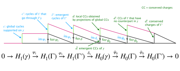
Figure 4: Long exact sequence and conserved charges/cycles of various types.

V.3 Reduction of buffering structures

Here we present the main result, regarding the reduction of buffering structures. The following theorem represents a particularly nice property of buffering structures under reductions. We show that the steady-state concentrations and rates of the network obtained by reducing a buffering structure are exactly the same as those of the network before reduction, without any modification of parameters. Thus, the reduction of a buffering structure preserves the steady-state properties of the boundary degrees of freedom. The theorem only relies on topological information of the network and is true regardless of the kinetics.

Theorem 4.

Let $\Gamma$ be a regular chemical reaction network with kinetics $\bm{r}(\bm{x})$ and let $\gamma$ be an output-complete subnetwork of $\Gamma$. We assume that the subnetwork $\gamma$ does not have an emergent conserved charge. We consider a reduced network $\Gamma^{\prime}=\Gamma/\gamma$. If $\gamma$ is a buffering structure, we have the isomorphisms,

$$\ker S/\ker S_{11}\cong\ker S^{\prime},\quad\mathop{{\rm coker}}S/\mathop{{\rm coker}}S_{11}\cong\mathop{{\rm coker}}S^{\prime},$$ (200)

Furthermore, when $(\bm{r},\bm{x})$ is steady-state reaction rates concentrations of $\Gamma$, whose components we separate into those in $\gamma$ and $\Gamma\setminus\gamma$ as

$$\bm{r}=\begin{pmatrix}\bm{r}_{1}\\ \bm{r}_{2}\end{pmatrix},\quad\bm{x}=\begin{pmatrix}\bm{x}_{1}\\ \bm{x}_{2}\end{pmatrix},$$ (201)

then, $(\bm{r}_{2},\bm{x}_{2})$ is a steady-state solution of $\Gamma^{\prime}$.

Remark 14.

Let us comment on the assumption of the absence of emergent conserved charges. Under the assumption of the regularity, the appearance of emergent conserved charges in an output-complete subnetwork $\gamma$ is quite unlikely. In fact, in the case of monomolecular reaction networks, we can prove $\widetilde{d}(\gamma)=0$ for a connected and output-complete subnetwork $\gamma$, assuming that $\Gamma$ is regular (see Appendix C.2), and this condition is redundant. So far, the examples of buffering structures with nonzero emergent conserved charges are pathological in some sense. Presently, we have not been able to prove the absence of emergent conserved charges for a generic (sound) reaction network, and thus it is assumed. We have more discussions on this point in Appendix C.

Remark 15.

We note that there is a possibility that the reduced system might have some solutions which are not allowed in the original system, depending on the kinetics. This can occur when the reactions in a subnetwork have limitations in the values of reaction rates. When such a subnetwork is removed, the reduced system does not have the restrictions, and there may appear additional solutions. Let us illustrate this with an example. We consider a reaction network $\Gamma=(\{v_{1},v_{2},v_{3}\},\{e_{1},e_{2},e_{3},e_{4},e_{5},e_{6},e_{7}\})$ given by the following set of reactions,

$$e_{1} :v_{1}\to v_{2},$$

$$e_{2} :v_{2}\to\text{(output)},$$

$$e_{3} :2v_{3}\to 3v_{3},$$

$$e_{4} :v_{3}\to\text{(output)},$$ (202)

$$e_{5} :\text{(input)}\to v_{3},$$

$$e_{6} :v_{3}\to v_{1}.$$

$$e_{7} :3v_{3}\to\text{(output)}.$$

Let us here choose the kinetics as

$$\begin{pmatrix}r_{1}(x_{1})\\ r_{2}(x_{2})\\ r_{3}(x_{3})\\ r_{4}(x_{3})\\ r_{5}\\ r_{6}(x_{3})\\ r_{7}(x_{3})\end{pmatrix}=\begin{pmatrix}\frac{k_{1}x_{1}}{c_{1}+x_{1}}\\ k_{2}x_{2}\\ k_{3}(x_{3})^{2}\\ k_{4}x_{3}\\ k_{5}\\ k_{6}x_{3}\\ k_{7}(x_{3})^{3}\end{pmatrix}.$$ (203)

For reaction $r_{1}$, we adopted the Michaelis-Menten kinetics, and we chose the mass-action kinetics for other reactions. The rate equations read

$$\frac{d}{dt}x_{1} =r_{6}(x_{3})-r_{1}(x_{1})=k_{6}x_{3}-\frac{k_{1}x_{1}}{c_{1}+x_{1}},$$ (204)

$$\frac{d}{dt}x_{2} =r_{1}(x_{1})-r_{2}(x_{2})=\frac{k_{1}x_{1}}{c_{1}+x_{1}}-k_{2}x_{2},$$ (205)

$$\frac{d}{dt}x_{3} =-k_{7}(x_{3})^{3}+k_{3}(x_{3})^{2}-k_{4}x_{3}+k_{5}-k_{6}x_{3}\eqqcolon-k_{7}(x_{3}-d_{1})(x_{3}-d_{2})(x_{3}-d_{3}),$$ (206)

where we reparametrized the equation for $\frac{d}{dt}x_{3}$ using $d_{1}$, $d_{2}$, and $d_{3}$ such that $d_{1}<d_{2}<d_{3}$. From Eq. (206), we get two candidates of stable steady-state values, $\bar{x}_{3}=d_{1},d_{3}$ (note that $d_{2}$ is unstable). However, those candidates may not lead to the solutions of whole equations when the reaction rate $r_{1}$ has a bound, as in the current example. Using Eq. (204), the steady-state value of $x_{1}$ is given by

$$\bar{x}_{1}=\frac{c_{1}k_{6}\bar{x}_{3}}{k_{1}-k_{6}\bar{x}_{3}}.$$ (207)

If the denominator of Eq. (207) is negative, it is not a valid solution. Thus, depending on the values of $d_{1}$ and $d_{3}$, the original network may have no, or one, or two solutions. The subnetwork $\gamma=\{(v_{1}),(e_{1})\}$ is a buffering structure, and we can consider the corresponding reduced network $\Gamma^{\prime}=\Gamma/\gamma$. In the reduced network, such a restriction on the values of (internal) reaction rates is invisible. Hence, the reduced system may admit more solutions that were not possible in the original system.

Proof.

The regularity of $\Gamma$ requires $\lambda(\gamma)\geq 0$ (Remark 8). In the absence of the emergent conserved charges, we have

$$\lambda(\gamma)=\widetilde{c}(\gamma)+d_{l}(\gamma)=0.$$ (208)

Since $\widetilde{c}(\gamma)$ and $d_{l}(\gamma)$ are nonnegative integers, we have $\widetilde{c}(\gamma)=0$ and $d_{l}(\gamma)=0$. Since $\widetilde{c}(\gamma)=0$, we can use the long exact sequence (184). Because there is no emergent conserved charge, $\widetilde{d}(\gamma)=0$, by assumption, the connecting map $\delta_{1}$ is a zero map in the long exact sequence. This proves Eq. (200).

Let us proceed to the latter part of the claim. The steady-state condition of $\Gamma$ is written as

$$S\bm{r}(\bm{x}) =0,$$ (209)

$$\bm{d}^{\bar{\alpha}}\cdot\bm{x} =\ell^{\bar{\alpha}}.$$ (210)

As usual, we divide the degrees of freedom to those in $\gamma$ and $\Gamma\setminus\gamma$. Then Eq. (209) is written as

$$\begin{pmatrix}S_{11}&S_{12}\\ S_{21}&S_{22}\end{pmatrix}\begin{pmatrix}\bm{r}_{1}(\bm{x}_{1},\bm{x}_{2})\\ \bm{r}_{2}(\bm{x}_{2})\end{pmatrix}=\bm{0}.$$ (211)

The reactions $\bm{r}_{2}(\bm{x}_{2})$ depend only on $\bm{x}_{2}$, because $\gamma$ is chosen to be output-complete. The first equation can be solved for $\bm{r}_{1}$ as $\bm{r}_{1}=-S_{11}^{+}S_{12}\bm{r}_{2}+\bm{c}_{11},$ with $\bm{c}_{11}\in\ker S_{11}$, and we have

$$S^{\prime}\bm{r}_{2}(\bm{x}_{2})=-S_{21}\bm{c}_{11}=\bm{0},$$ (212)

where the last equality is due to $\widetilde{c}(\gamma)=0$, that is equivalent to $\ker S_{11}\subset\ker S_{21}$.

Let us turn to the conserved charges. Recall that $d_{l}(\gamma)$ is written as $d_{l}(\gamma)=|(\mathop{{\rm coker}}S)/X(\gamma)|$. Because of the decomposition (165), when $d_{l}(\gamma)=0$, the space $\mathop{{\rm coker}}S$ is written as the direct sum of $D(\gamma)$ and $\bar{D}^{\prime}(\gamma)$,

$$\mathop{{\rm coker}}S\cong D(\gamma)\oplus(\mathop{{\rm coker}}S)/X(\gamma)\oplus\bar{D}^{\prime}(\gamma)\cong D(\gamma)\oplus\bar{D}^{\prime}(\gamma).$$ (213)

Correspondingly, we can divide the basis vectors of $\mathop{{\rm coker}}S$ into two classes, $\{\bm{d}^{\bar{\alpha}}\}=\{\bm{d}^{\bar{\alpha}_{\gamma}},\bm{d}^{\bar{\alpha}^{\prime}}\}$, where $\{\bm{d}^{\bar{\alpha}_{\gamma}}\}$ is a basis of $D(\gamma)$, and $\{\bm{d}^{\bar{\alpha}^{\prime}}\}$ is a basis of $\bar{D}^{\prime}(\gamma)$. The basis vectors are of the form,

$$\bm{d}^{\bar{\alpha}_{\gamma}}=\begin{pmatrix}\bm{d}^{\bar{\alpha}_{\gamma}}_{1}\\ \bm{d}^{\bar{\alpha}_{\gamma}}_{2}\end{pmatrix}\text{ with }\bm{d}^{\bar{\alpha}_{\gamma}}_{1}\neq\bm{0},\quad\bm{d}^{\bar{\alpha}^{\prime}}=\begin{pmatrix}\bm{0}\\ \bm{d}^{\bar{\alpha}^{\prime}}_{2}\end{pmatrix}.$$ (214)

With this basis of $\mathop{{\rm coker}}S$, Eq. (210) is written as

$$\bm{d}_{1}^{\bar{\alpha}_{\gamma}}\cdot\bm{x}_{1}+\bm{d}_{2}^{\bar{\alpha}_{\gamma}}\cdot\bm{x}_{2} =\ell^{\bar{\alpha}_{\gamma}},$$ (215)

$$\bm{d}_{2}^{\bar{\alpha}^{\prime}}\cdot\bm{x}_{2} =\ell^{\bar{\alpha}^{\prime}}.$$ (216)

In fact, $\bm{d}^{\bar{\alpha}^{\prime}}_{2}$ is a conserved charge in $\Gamma^{\prime}$, $\bm{d}^{\bar{\alpha}^{\prime}}_{2}\in\mathop{{\rm coker}}S^{\prime}$, as we see in the following. Since $\bm{d}^{\bar{\alpha}^{\prime}}\in\mathop{{\rm coker}}S$ , it satisfies

$$\begin{pmatrix}\bm{0}&(\bm{d}^{\bar{\alpha}^{\prime}}_{2})^{T}\end{pmatrix}\begin{pmatrix}S_{11}&S_{12}\\ S_{21}&S_{22}\end{pmatrix}=\begin{pmatrix}(\bm{d}^{\bar{\alpha}^{\prime}}_{2})^{T}S_{21}&(\bm{d}^{\bar{\alpha}^{\prime}}_{2})^{T}S_{22}\end{pmatrix}=\bm{0}.$$ (217)

This implies that $\bm{d}^{\bar{\alpha}^{\prime}}_{2}$ satisfies

$$(\bm{d}^{\bar{\alpha}^{\prime}}_{2})^{T}S^{\prime}=(\bm{d}^{\bar{\alpha}^{\prime}}_{2})^{T}(S_{22}-S_{21}S^{+}_{11}S_{12})=\bm{0},$$ (218)

hence $\bm{d}^{\bar{\alpha}^{\prime}}_{2}\in\mathop{{\rm coker}}S^{\prime}$. Thus we have obtained an injective map,

$$\mathop{{\rm coker}}S\ni\bm{d}^{\bar{\alpha}^{\prime}}=\begin{pmatrix}\bm{0}\\ \bm{d}^{\bar{\alpha}^{\prime}}_{2}\end{pmatrix}\mapsto\bm{d}^{\bar{\alpha}^{\prime}}_{2}\in\mathop{{\rm coker}}S^{\prime}.$$ (219)

This map is nothing but the induced map $\bar{\varphi}_{0}$. It is important to note that, when $\widetilde{c}(\gamma)=0$, this map is a surjection, that is evident from the long exact sequence (184). The equations satisfied by the boundary part (denoted by 2) of the concentrations/rates of $\Gamma$ are Eqs. (212) and (216). Since all the conserved charges in $\Gamma^{\prime}$ is given as a image $\bar{\varphi}_{0}$, we find that the set of Eqs. (212) and (216) are exactly the same as the steady-state condition for the reduced network $\Gamma^{\prime}$,

$$S^{\prime}\bm{r}^{\prime}(\bm{x}^{\prime}) =\bm{0},$$ (220)

$$\bm{d}_{2}^{\bar{\alpha}^{\prime}}\cdot\bm{x}^{\prime} =\ell^{\bar{\alpha}^{\prime}}.$$ (221)

where $\bm{x}^{\prime}=\bm{x}_{2}$ and $\bm{r}^{\prime}(\bm{x}^{\prime})=\bm{r}_{2}(\bm{x}_{2})$. Thus, the steady-state solution of $\Gamma^{\prime}$ should also be the steady-state solution of $\Gamma$ for the boundary degrees of freedom. This concludes the proof. ∎

V.4 Hierarchy of subnetworks

Let us consider nested subnetworks $\gamma^{\prime}\subset\gamma\subset\Gamma$. Given the stoichiometric matrix $S$ of the whole network, we denote the stoichiometric matrices of the subnetworks $\gamma$ and $\gamma^{\prime}$ by $S_{\gamma}$ and $S_{\gamma^{\prime}}$, respectively. The submatrices are included in the following form,

$$S=\begin{pmatrix}S_{\gamma}&\ast\\ \ast&\ast\end{pmatrix},\quad S_{\gamma}=\begin{pmatrix}S_{\gamma^{\prime}}&\ast\\ \ast&\ast\end{pmatrix},$$ (222)

where $\ast$ indicates an arbitrary matrix. Let us consider the situation where $\gamma$ and $\gamma^{\prime}$ has no emergent cycle and emergent conserved charge in $\Gamma$, namely $\widetilde{c}(\gamma)=\widetilde{d}(\gamma)=0$, and $\widetilde{c}(\gamma^{\prime})=\widetilde{d}(\gamma^{\prime})=0$. Under those assumptions, the quotient formula of the generalized Schur complement [57] holds,

$$S/S_{\gamma}=(S/S_{\gamma^{\prime}})/(S_{\gamma}/S_{\gamma^{\prime}}).$$ (223)

This indicates the isomorphisms of homology groups,

$$H_{n}(\Gamma/\gamma)\cong H_{n}((\Gamma/\gamma^{\prime})/(\gamma/\gamma^{\prime})),$$ (224)

for $n=0,1$. Thus, when we perform the reductions of nested subnetworks that have no emergent cycles and emergent conserved charges, the order of the reduction of them does not matter.

VI Example of reduction: metabolic pathway of E. coli

As an application of the reduction method, let us examine the central metabolism of E. coli. We use the stoichiometric matrix presented in Ref. [45], which is constructed based on Ref. [4] with minor modifications. The network structure is shown in Fig. 5a, which consists of the glycolysis, the pentose phosphate pathway (PPP), and the tricarboxylic acid cycle (TCAC). The list of the reactions for this system is given in Appendix D.1. Here, we assume that H₂O and cofactors such as ATP and NADH are abundant and do not affect the behavior of the system. Buffering structures in this network have been identified in Ref. [24] and there are in total 17 buffering structures, which we list in Appendix D.2. As we showed in Sec. III.3, the intersections or unions of buffering structures are also buffering structures. They form a hierarchy, and such an architecture can be regarded as a source of robustness against perturbations, since buffering structures work as a kind of firewalls.

Let us now perform reductions of buffering structures, under which the steady state is ensured to be the same as the original network as we showed in Sec. V.3. We denote the whole network by $\Gamma$. We can pick a buffering structure $\gamma_{8}$, which is a part of the pentose phosphate pathway (the yellow subnetwork in Fig. 5a) and given by

$$\gamma_{8}=(\{\text{X5P, S7P, E4P}\},\{17,18,19,20,21\}),$$ (225)

and perform a reduction to obtain $\Gamma_{1}\coloneqq\Gamma/\gamma_{8}$. The stoichiometric matrix of the reduced reaction network can be computed by Eq. (101). The resulting network is shown in Fig. 5b. The reduction procedure induces rewiring of the reactions, which are colored in magenta in Fig. 5. Reactions 15 and 22 are rewired, and 22 is now a degenerate reaction. The fraction $1/2$ shown at reaction 15 indicates the weight of the species. Those reconnections including the change of weights are necessary if we want the steady state to be the same as those of the original network. Otherwise, the steady state is changed in general. We can proceed further and reduce the subnetwork $(\{\text{G3P,R5P}\},\{7,22,40\})$ (colored in red and orange in Fig. 5a). This reduction is the same as reducing $\gamma_{5}\cup\gamma_{14}$ from $\Gamma$. The result of the reduction is shown in Fig. 5c. Again, rewiring occurs and the reactions 5,6,15, and 36 are modified from the original system. Finally, let us focus on the part colored in green in Fig. 5a, which consists of the following subsets of chemical species and reactions,

$$(\{\text{G6P},\text{F6P},\text{F16P},\text{6PG},\text{Ru5P},\text{DHAP}\},\{2,3,4,5,6,13,14,15,16,36,43\}).$$ (226)

The complement of the subset (226) is given by $\gamma_{5}\cup\gamma_{7}\cup\gamma_{14}$, which hence is a buffering structure, and a reduction can be performed. The structure of the reduced network $\Gamma_{3}=\Gamma/(\gamma_{5}\cup\gamma_{7}\cup\gamma_{14})$ is given in Fig. 5d. Compared to the original network, we notice that the reactions 15 and 43 are rewired.

To demonstrate our theoretical prediction, we numerically solve the rate equations for the four systems in Fig. 5 (the original network $\Gamma$ and the reduced ones, $\Gamma_{1},\,\Gamma_{2},\,\Gamma_{3}$), using the same initial condition and reaction rate constants in all of the four cases (see Appendix D.3 for details of parameter values). The time-series of concentrations are presented in Fig. 6. After the initial transient dynamics, the original system approaches a (stable) steady state [Fig. 6(a)]. We can see that the reduced systems can reproduce the steady-state concentrations that the original system eventually reaches, although they have distinct short-time dynamics [Fig. 6(b-d)].

In this way, buffering structures work as a guide as to how to perform the reduction and simplify a complex reaction network. As long as the reduced part is a buffering structure and we use the generalized Schur complement (101) as a stoichiometric matrix of a reduced network, the steady-state concentrations and rates of the remaining part stay the same as the original ones regardless of the details of the kinetics, as a consequence of Theorem 201.

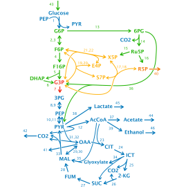
(a)

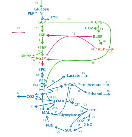
(b)

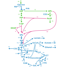
(c)

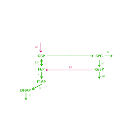
(d)

Figure 5: Central metabolic pathway (a) of E. coli and reduced networks (b, c, d). In the reduced networks, rewired reactions under the reductions are colored in magenta. (b) Reduced network $\Gamma_{1}=\Gamma/\gamma_{8}$, where $\gamma_{8}$ is colored in yellow in (a). The fraction $1/2$ written in black indicates the weight in the stoichiometric matrix. (c) $\Gamma_{2}=\Gamma/(\gamma_{5}\cup\gamma_{14})$, where $\gamma_{5}\cup\gamma_{14}$ is colored in yellow, red, and orange in (a). (d) $\Gamma_{3}=\Gamma/(\gamma_{5}\cup\gamma_{7}\cup\gamma_{14})$, where $\gamma_{5}\cup\gamma_{7}\cup\gamma_{14}$ is colored in yellow, red, orange, and blue in (a).

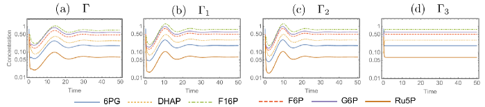
Figure 6: Time-series of concentrations of DHAP, F16P, F6P, G6P, PG6, Ru5P computed by solving the whole system $\Gamma$ (a) and the reduced systems $\Gamma_{1},\,\Gamma_{2},\,\Gamma_{3}$ (b, c, d). The same initial condition and reaction rate constants are used in the four cases.

VII Summary and outlook

The main focus of the present paper was the relationship between the structure and functions of the chemical reaction network. As a characterization of the structure, homology and cohomology groups for chemical reaction networks were introduced, in which the actions of boundary and coboundary operators are determined by the stoichiometry. The elements of homology groups correspond to cycles and conserved charges of chemical reaction networks, and steady states were shown to be determined by the elements of the cohomology groups. In a similar way to the homology and cohomology groups of topological spaces, the Mayer-Vietoris sequence and the long exact sequence of a pair of chemical reaction networks were introduced, the latter being particularly useful for studying the reduction of reaction networks.

We propose a method of reduction of chemical reaction networks. The reduced network is characterized by the stoichiometric matrix obtained by eliminating the chemical species and reactions of an output-complete subnetwork via the Schur complementation. The reduction relies only on the stoichiometry, which determines the topology of the reaction networks, and thus is applicable to any kind of kinetics. This represents an advantage since in many biological systems it is difficult to experimentally determine the kinetics and parameters of the reactions. For tracking the change of cycles and conserved charges under the reductions, the tools of algebraic topology, such as the long exact sequence, have been useful. We have studied how the law of localization can be understood from this perspective. We showed that the influence index is expressed in terms of the numbers of cycles/conserved charges of particular types, as in Eq. (172). We also showed that the influence index is a submodular function over output-complete subnetworks. A corollary of this is that buffering structures are closed under intersection and union, which is useful when we enumerate the buffering structures of a large reaction network. As a central result of the paper, we showed that buffering structures, which are subnetworks with vanishing influence index, behave nicely under the reduction. Namely, under the reduction of a buffering structure, the steady state of the remaining elements of the network stays the same as the original network (Theorem 201). The theorem justifies the intuition that buffering structures are regarded as ‘irrelevant’ substructures: they can be safely eliminated through the reduction method proposed here without changing the long-time behavior of the system. The reduction procedure introduces rewiring of reactions, which is necessary so that the steady state is not modified under the reduction. As an application of the reduction method, we discussed the reduction of the central metabolic pathway of E. coli and illustrated that reactions are rewired non-trivially under the reduction. We also demonstrated the invariance of the steady state under the reduction of buffering structures by numerically solving the rate equations before and after the reduction.

Our results highlight that special care should be taken when simplifying a reaction network. A naive elimination of a subnetwork not of interest would alter steady-state properties of the original system. As long as the subnetwork has the vanishing influence index and reactions are rewired appropriately using the generalized Schur complement, it can be eliminated while keeping the steady state intact.

Another significance of our method is that it allows us to identify the modules in a complex network and facilitates the biological interpretation of the whole system. For example, the central metabolic pathway of E. coli consists of three modules; glycolysis, TCAC, and PPP. Interestingly, the reduced network in Fig. 5d roughly corresponds to the glycolysis. The fact of glycolysis being a reduced network may suggest that E. coli can control the glycolysis in an isolated manner, and the expression levels of enzymes in the TCAC and the PPP do not affect the physiological states of the glycolysis.

For practical applications, one important issue is how to find the buffering structures efficiently in large-scale reaction networks. Although we defer this as a future problem, let us make some comments on this point. One practical way of finding buffering structures is as follows: We first compute the sensitivity matrix $A^{-1}$ by assigning random values to $\frac{\partial r_{A}}{\partial x_{i}}$. From this, we can identify, for each parameter $k_{A}$ (and for each conserved concentration $l^{\bar{\alpha}}$ if exists), the subset $V_{A}$ of chemicals that show nonzero responses to the perturbation of $k_{A}$ under generic kinetics. The inclusion relation among $V_{A}$’s indicates candidate buffering structures (see Figs. 3 and 5 in [24] for the illustrations). For example, $V_{A}\subset V_{B}$ indicates the existence of two nested buffering structures. Finally, for those candidates, we can compute the influence index and verify if they are indeed buffering structures.

Establishing a combinatorial method for identifying buffering structures is an amusing problem. We believe that the basic properties of buffering structures that we showed in this paper would be useful for this purpose. For example, if a network contains many small buffering structures, we can use the reduction method repeatedly and make the network smaller one we fine a small buffering structure. This procedure is possible because the order of reduction does not matter for the buffering structures, as we showed in Sec. V.4. The submodular property of the influence index and the subsequent closure property of buffering structures under unions/intersections would also be useful in enumerating buffering structures.

We believe that the mathematical formulation that we used to characterize the topology of chemical reaction networks will be useful for understanding the static and dynamical properties of reaction systems. The eigenvalues of the Laplacian operators entail the information of the topology of the network connectivity. Steady states correspond to the eigenvectors with zero eigenvalues and they incorporate the crudest topological information of the reaction network. The eigenvectors with higher eigenvalues are going to be needed if we want to extend the reduction method to approximate the dynamics as well as the steady states.

Appendix A Laplace operators and Hodge decomposition

In this section, we discuss the Hodge decomposition and Laplace operators, which are closely related to the cohomology groups introduced in the main text.

We can define Laplace operators, $\Delta_{n}:C^{n}(\Gamma)\to C^{n}(\Gamma)$, as

$$\Delta_{0}\coloneqq{\rm d}^{\dagger}_{0}{\rm d}_{0},\quad\Delta_{1}\coloneqq{\rm d}_{0}{\rm d}^{\dagger}_{0}.$$ (227)

Recall that the coboundary operator (19) and its adjoint (23) are given by $({\rm d}_{0}a_{0})(e_{A})=\sum_{i}(S^{T})_{Ai}a_{0}(v_{i})$ for $a_{0}\in C^{0}(\Gamma)$ and $({\rm d}^{\dagger}_{0}a_{1})(v_{i})=\sum_{A}S_{iA}a_{1}(e_{A})$ for $a_{1}\in C^{1}(\Gamma)$. The action of the Laplacians are written in the matrix form as

$$(\Delta_{0}a_{0})(v_{i})=\sum_{j}(SS^{T})_{ij}\,a_{0}(v_{j}),\quad(\Delta_{1}a_{1})(e_{A})=\sum_{B}(S^{T}S)_{AB}\,a_{1}(e_{B}),$$ (228)

for $a_{0}\in C^{0}(\Gamma)$ and $a_{1}\in C^{1}(\Gamma)$. Those are generalizations of the graph Laplacian to hypergraphs. The properties of hypergraph Laplacians were discussed recently in Refs. [58, 59, 60]. When all the reactions are monomolecular, the Laplacian reduces to the graph Laplacian of the directed graph.

The space $C^{1}(\Gamma)$ admits the following orthogonal decomposition,

$$C^{1}(\Gamma)={\rm im\,}{\rm d}_{0}\oplus\ker\Delta_{1}.$$ (229)

This is a natural generalization of the Hodge decomposition of flows on networks [61] to the case of a hypergraph. Thus, given a 1-cochain $f\in C^{1}(\Gamma)$, we can decompose it in a unique way as

$$f={\rm d}_{0}a+c,$$ (230)

where $c\in\ker{\rm d}_{0}^{\dagger}\,\cap\,\ker{\rm d}_{1}$ is a harmonic cochain and $a\in C^{0}(\Gamma)$. This is the Hodge decomposition associated with the complex (27). By acting ${\rm d}^{\dagger}_{0}$ on Eq. (230), we have

$${\rm d}^{\dagger}_{0}f={\rm d}^{\dagger}_{0}{\rm d}_{0}a=\Delta_{0}a.$$ (231)

We can solve this for the potential $a$ as

$$a=\Delta_{0}^{+}{\rm d}^{\dagger}_{0}f+a_{0}.$$ (232)

Here, $\Delta_{0}^{+}:C^{0}(\Gamma)\to C^{0}(\Gamma)$ is the operator defined by $(\Delta^{+}_{0}b_{0})(v_{i})\coloneqq\sum_{j}(SS^{T})^{+}_{ij}b_{0}(v_{j})$ for $b_{0}\in C^{0}(\Gamma)$, where $M^{+}$ indicates the Moore-Penrose inverse of a matrix $M$, and $a_{0}\in\ker\Delta_{0}$. The harmonic component $c$ can be obtained by

$$c=f-{\rm d}_{0}a=(1-{\rm d}_{0}\Delta^{+}_{0}{\rm d}^{\dagger}_{0})f.$$ (233)

Using the properties of the Moore-Penrose inverse, the action of the operator that appears on the RHS of Eq. (233) is written as

$$[(1-{\rm d}_{0}\Delta^{+}_{0}{\rm d}^{\dagger}_{0})b_{1}](e_{A})=\sum_{B}(1-S^{+}S)_{AB}\,b_{1}(e_{B}),$$ (234)

for an arbitrary $b_{1}\in C^{1}(\Gamma)$. The matrix $1-S^{+}S$ is the projection matrix to $\ker S$. Thus, the harmonic component can be identified by the projection to $\ker S$,

$$c(e_{A})=\sum_{B}(1-S^{+}S)_{AB}f(e_{B}).$$ (235)

This is consistent with the fact that $c\in H^{1}(\Gamma)=\ker S$. The potential $a$ can be obtained by the multiplication of the Moore-Penrose inverse of $S$ to $f$,

$$a(v_{i})=\sum_{A}(S^{T})^{+}_{iA}f(e_{A})+a_{0}(v_{i}),$$ (236)

where $a_{0}\in\ker\Delta_{0}$.

Appendix B Cycles and conserved charges

B.1 Interpretation of $\widetilde{c}(\gamma)$ and $d_{l}(\gamma)$, and $\widetilde{d}(\gamma)$

Let us here discuss intuitive interpretations of the integers appearing in the decomposition (172). We will refer to the elements of $\ker S$ as “global cycles” and those of $\mathop{{\rm coker}}S$ as “global conserved charges.” Similarly, the elements $\ker S_{11}$ and $\mathop{{\rm coker}}S_{11}$ are referred to as “local cycles” and “local conserved charges.” With this terminology, the elements of $(\ker S)_{{\rm supp}\,\gamma}$ are called as “locally supported global cycles.”

We first look at $\widetilde{c}(\gamma)$. We denote the space by

$${\rm\widetilde{C}}(\gamma)\coloneqq\ker S_{11}/(\ker S)_{{\rm supp}\,\gamma}.$$ (237)

Then, $\widetilde{c}(\gamma)=|{\rm\widetilde{C}}(\gamma)|$. To clarify its meaning, we represent the space (237) as follows,

$$\begin{split}{\rm\widetilde{C}}(\gamma)&=\{\bm{c}\in C_{1}(\Gamma)\,|\,S\bm{c}=\bar{P}^{0}_{\gamma}\bm{v},\,P^{1}_{\gamma}\bm{c}=\bm{c}\}/\{\bm{c}\in C_{1}(\Gamma)\,|\,S\bm{c}=0,\,P^{1}_{\gamma}\bm{c}=\bm{c}\}\\ &=\{\bm{c}\in C_{1}(\Gamma)\,|\,S\bm{c}=\bm{v}\neq\bm{0},\,\bm{v}\in C_{0}(\Gamma\setminus\gamma),\,P^{1}_{\gamma}\bm{c}=\bm{c}\}.\end{split}$$ (238)

An element of ${\rm\widetilde{C}}(\gamma)$ is a local cycle that is not a global cycle, by which we mean that $\bm{c}\in{\rm\widetilde{C}}(\gamma)$ has its boundary in $\Gamma\setminus\gamma$. For example, let us take the subnetwork $\gamma=(\{v_{2}\},\{e_{1},e_{2}\})$ of a monomolecular reaction network,

(239)

Although $e_{1}+e_{2}\in C_{1}(\Gamma)$ has its support in $\gamma$, its boundary,

$$\partial_{1}(e_{1}+e_{2})=-v_{1}+v_{3},$$ (240)

is outside of $\gamma$. The element $e_{1}+e_{2}$ is a local cycle, since $\partial_{1}(e_{1}+e_{2})$ is zero as a relative chain in $C_{0}(\gamma)=C_{0}(\Gamma)/C_{0}(\Gamma\setminus\gamma)$. Note that the network (239) as a whole does not have a cycle and $\ker S=\bm{0}$. Thus, we can identify $\bm{c}\in{\rm\widetilde{C}}(\gamma)$ to be a local cycle whose boundary is out of $\gamma$. When $\bm{c}$ is viewed in $\Gamma$, it may be extended to a global cycle, but it does not have to be. Considering its meaning, we will refer to the elements of ${\rm\widetilde{C}}(\gamma)$ as emergent cycles, which only appear when we focus on a subnetwork.

Let us illustrate the space ${\rm\widetilde{C}}(\gamma)$ pictorially. The matrix $S$ works as a boundary operator on the space of chemical reactions. Thus, the kernel of $S$ are linear combinations of reactions without boundaries. Cycles and non-cycles can be drawn pictorially as

,

where the boundary of the box is identified.

We consider an output-complete subnetwork $\gamma$. The space ${\ker}\,S_{11}$ is spanned by local cycles in $\gamma$, for example,

,

where the inner box represents a subnetwork $\gamma$ and the red lines constitute the basis of the space. Here, the symbol means that the cut ends are reactions and not chemical species. See the following two choices for example:

For the left one, cut ends are both reactions. For the right one, the cut ends are a species and a reaction. Both ends have to be reactions so that the cut cycle can be a local cycle. An element of $\ker S_{11}$ may be extended to a global cycle, or it may be a part of a global noncycle.

The space $({\ker}S)_{{\rm supp}\,\gamma}$ for the same configuration takes into account only the global cycles supported on $\gamma$,

.

Therefore, the coset space is generated by the following elements,

.

As we see in the figure, the space $\ker S_{11}/(\ker S)_{{\rm supp}\,\gamma}$ consists of local cycles that are not global cycles.

We can similarly interpret conserved charges. The transpose of the stoichiometric matrix, $S^{T}$, can be regarded as a boundary operator acting on $C_{0}(\Gamma)$, which is the space of chemical species. In this sense, an element of $\mathop{{\rm coker}}S$ has no boundary, with respect to this boundary operator. We here visualize this in a similar way to the cycles,

.

Note that the boundary of the box is identified. The filled circles represent a source or a drain of chemical species, because of which the charge is not conserved.

The space $\mathop{{\rm coker}}S$ represents the global conserved charges, and $P^{0}_{\gamma}(\mathop{{\rm coker}}S)$ is the projection of $\mathop{{\rm coker}}S$ to $\gamma$,

.

Here, how the conserved charges are cut does not matter. The space $\mathop{{\rm coker}}S_{11}$ is generated by the red and green elements in the following figure,

,

where filled and open rectangles mean boundaries with chemical species and reactions, respectively. The parts we denoted by green lines, , are emergent conserved charges, which are conserved when it is seen in a subnetwork but not conserved in $\Gamma$. In fact, the appearance of emergent conserved charges typically leads to “unphysical” systems, in the sense that either a steady state does not exist or the matrix $A$ is not invertible and the response of the system to the perturbation of parameters is not well-defined. For example, one can consider the following network and subnetwork,

The whole network does not have a conserved charge, but the subnetwork $\gamma$ has one, $v_{1}+v_{2}+v_{3}$. However, such a reaction network cannot reach a steady state, since the concentration of $v_{3}$ continues to increase. When we take the difference $|P^{0}_{\gamma}(\mathop{{\rm coker}}S)|-|\mathop{{\rm coker}}S_{11}|$ , we can count the number of lost conserved charges minus the number of emergent conserved charges (if any),

,

where the part colored in red in the first term indicates lost conserved charges, that are conserved in $\Gamma$ but their projections to $\gamma$ are not. This equation is equal to the latter two terms of the decomposition (172), $d_{l}(\gamma)-\widetilde{d}(\gamma)$.

Example 11.

Consider a monomolecular network $\Gamma=(V,E)=(\{v_{1},v_{2},v_{3}\},\{e_{1},e_{2}\})$ with the following structure,

We take a subnetwork $\gamma_{1}=(\{v_{2}\},\{e_{1},e_{2}\})$ that is indicated by a box. The whole network does not have a cycle, and the subnetwork $\gamma_{1}$ has one emergent cycle given by $c=e_{1}+e_{2}$. Also, $\Gamma$ has one conserved charge, $d=v_{1}+v_{2}+v_{3}$. Its projection to $\gamma_{1}$ is given by $v_{2}$ and it is not a conserved charge in $\gamma_{1}$. So we have one lost conserved charge. Each integer appearing in the decomposition of $\lambda(\gamma_{1})$ is

$$\widetilde{c}(\gamma_{1})=1,\quad d_{l}(\gamma_{1})=1,\quad\widetilde{d}(\gamma_{1})=0,$$ (241)

and $\lambda(\gamma_{1})=2$. For the same $\Gamma$, let us consider a different choice of a subnetwork,

The subnetwork $\gamma_{2}$ does not have a cycle, and there is one lost conserved charge, so we have

$$\widetilde{c}(\gamma_{2})=0,\quad d_{l}(\gamma_{2})=1,\quad\widetilde{d}(\gamma_{2})=0,\quad\lambda(\gamma_{2})=1.$$ (242)

Example 12.

Consider a network $(V,E)=(\{v_{1},v_{2},v_{3}\},\{e_{1},e_{2},e_{3}\})$ with the following structure,

If we choose a subnetwork $\gamma=(\{v_{3}\},\{e_{2},e_{3}\})$,

$$\widetilde{c}(\gamma)=1,\quad d_{l}(\gamma)=1,\quad\widetilde{d}(\gamma)=0,\quad\lambda(\gamma)=2.$$ (243)

The subnetwork $\gamma$ has one emergent cycle and one lost conserved charge and the influence index is $2$.

B.2 Embedding of A-matrices

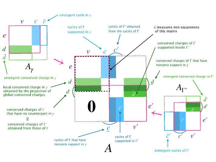
Figure 7: Embedding of the A-matrices for a generic output-complete subnetwork.

It is useful to look at the A-matrix to visualize the relations among cycles/conserved charges of various types in subnetworks and reduced networks.

Let us first summarize the notations. In this section, we suppress the dependence on $\gamma$ for notational simplicity. General rules are as follows. Quantities with a tilde are emergent ones, and we use character $c$ for cycles and $d$ for conserved charges. The numbers with a prime are associated with $\Gamma^{\prime}$. The relevant numbers are listed as follows:

• $v,v^{\prime}$: number of chemical species in $\gamma,\Gamma^{\prime}$

• $e,e^{\prime}$: number of chemical reactions in $\gamma,\Gamma^{\prime}$

• $\widetilde{c},\widetilde{c}^{\prime}$: number of emergent cycles of $\gamma,\Gamma^{\prime}$

• $\widetilde{d},\widetilde{d}^{\prime}$: number of emergent conserved charges of $\gamma,\Gamma^{\prime}$

• $c,c^{\prime}$: number of cycles of $\Gamma$, whose projections to $\gamma,\Gamma^{\prime}$ are also cycles of $\gamma,\Gamma^{\prime}$

• $d,d^{\prime}$: number of conserved charges of $\Gamma$, whose projections to $\gamma,\Gamma^{\prime}$ are also conserved in $\gamma,\Gamma^{\prime}$

• $\bar{c}^{\prime},\bar{d}^{\prime}$: number of cycles/conserved charges of $\Gamma$ that are locally supported in $\Gamma^{\prime}$

• $\underline{c},\underline{d}$: number of cycles/conserved charges of $\Gamma$ that have nonzero support in $\gamma$

In Fig. 7, we illustrate a more detailed structure of the matrix $A$ than Fig. 3. In the center is the matrix $A$ of the total system $\Gamma$. We choose an output-complete subnetwork $\gamma$, and bring the rows/columns related to $\gamma$ to the upper-left part. Then the matrix $A$ looks like one in the center of Fig. 7. We consider an output-complete subnetwork $\gamma$, and the A-matrix of $\gamma$, which we denote by $A_{\gamma}$, is shown in the upper-left part of Fig. 7. The part surrounded by a pink rectangle is the common part of $A_{\gamma}$ and $A$. The subnetwork $\gamma$ can in general contain additional (i.e., emergent) cycles and conserved charges, whose numbers are denoted by $\widetilde{c}$ and $\widetilde{d}$. Because the matrix $A_{\gamma}$ is square, we have the relation,

$$e+d+\widetilde{d}=v+c+\widetilde{c}.$$ (244)

This equation is in fact the same as Eq. (51). Similarly, we can consider the matrix $A$ for the network $\Gamma^{\prime}=\Gamma/\gamma$ obtained by reducing $\gamma$ from $\Gamma$. The numbers of the emergent cycles and emergent conserved charges in $\Gamma^{\prime}$ are denoted by $\widetilde{c}^{\prime}$ and $\widetilde{d}^{\prime}$. The matrix $A_{\Gamma^{\prime}}$ is also square and we have

$$e^{\prime}+d^{\prime}+\widetilde{d}^{\prime}=v^{\prime}+c^{\prime}+\widetilde{c}^{\prime}.$$ (245)

The influence index is given by

$$\lambda\coloneqq e+d+d^{\prime}-\bar{d}^{\prime}-v-c,$$ (246)

which measures how far the rectangle in the upper-left part (indicated by black dashed lines) is from a square matrix. Note that this expression is consistent with the one in Sec. III.2 since $\underline{d}=d+d^{\prime}-\bar{d}^{\prime}$. Using Eq. (244), we can also express $\lambda$ as

$$\lambda=\widetilde{c}+d^{\prime}-\bar{d}^{\prime}-\widetilde{d},$$ (247)

which is the same the decomposition (172). We can also consider a similar quantity that measure the non-squareness of the lower-right part,

$$\lambda^{\prime}\coloneqq v^{\prime}+c^{\prime}-e^{\prime}-\bar{d}^{\prime}=\widetilde{d}^{\prime}+d^{\prime}-\bar{d}^{\prime}-\widetilde{c}^{\prime},$$ (248)

where the second expression is obtained using Eq. (245). In fact, due to the squareness of the whole matrix $A$, $\lambda^{\prime}$ is equal to the influence index, $\lambda=\lambda^{\prime}$. This results in the following relation,

$$\widetilde{c}-\widetilde{d}+\widetilde{c}^{\prime}-\widetilde{d}^{\prime}=0.$$ (249)

Appendix C Emergent conserved charges in chemical reaction networks

In this section, we discuss the role of emergent conserved charges in chemical reaction networks.

C.1 Systems with emergent conserved charges

As far as we observe, the chemical reaction systems with emergent conserved charges in output-complete subnetworks are pathological, in either of the following senses:

• The steady-state condition,

  $$\sum_{A}S_{iA}r_{A}(\bm{x}(\bm{k},\bm{\ell}),k_{A})=0,\quad\sum_{i}d_{i}^{\bar{\alpha}}x_{i}=\ell^{\bar{\alpha}},$$ (250)

  does not fully determine the steady-state solution, and arbitrary parameters have to be introduced to specify the solution.

• No steady-state solution exists.

• The reaction kinetics is unphysical.

Below, we discuss some examples of each case.

C.1.1 Pattern A : solutions have arbitrary parameters

An example of pattern (A) is given by

$$\frac{d}{dt}\begin{pmatrix}x\\ y\end{pmatrix}=\begin{pmatrix}1&0\\ -1&-1\end{pmatrix}\begin{pmatrix}r_{1}\\ r_{2}\end{pmatrix},\quad\,\,\,\begin{pmatrix}r_{1}\\ r_{2}\end{pmatrix}=\begin{pmatrix}k_{1}y\\ k_{2}y\end{pmatrix}.$$ (251)

The matrix $A$ for this system is

$$A=\begin{pmatrix}0&k_{1}\\ 0&k_{2}\end{pmatrix}.$$ (252)

This is not invertible. The steady-state solution for the mass-action kinetics is given by

$$\begin{pmatrix}\bar{r}_{1}\\ \bar{r}_{2}\end{pmatrix}=\bm{0},\quad\begin{pmatrix}\bar{x}\\ \bar{y}\end{pmatrix}=\begin{pmatrix}m\\ 0\end{pmatrix},$$ (253)

where $m$ is an arbitrary parameter. If we choose a subnetwork $\gamma=\{x\}$, there is an emergent conserved charge. Let us consider the fluctuations around the steady state,

$$\frac{d}{dt}\begin{pmatrix}\delta x\\ \delta y\end{pmatrix}=\begin{pmatrix}1&0\\ -1&-1\end{pmatrix}\begin{pmatrix}k_{1}\delta y\\ k_{2}\delta y\end{pmatrix}=\begin{pmatrix}k_{1}\delta y\\ -(k_{1}+k_{2})\delta y\end{pmatrix},$$ (254)

where $\delta x(t)\coloneqq x(t)-\bar{x}$ indicates the fluctuation from the steady state. The fluctuation associated with the emergent charge, $\delta x$, is a zero mode. This means that the system is not asymptotically stable.

Generically, when we have to introduce arbitrary parameters $\bm{m}$, the matrix $A$ has a null vector, as we see below. The steady-state condition reads

$$r_{A}(\bm{x}(\bm{k},\bm{\ell},\bm{m}),\bm{k}) = -\sum_{\alpha}\mu_{\alpha}(\bm{k},\bm{\ell},\bm{m})c^{\alpha}_{A},$$ (255)

$$\sum_{i}d^{\bar{\alpha}}_{i}x_{i}(\bm{k},\bm{\ell},\bm{m}) = \ell^{\bar{\alpha}}.$$ (256)

By taking the derivative of those equations with respect to $\bm{m}$, we find

$$\begin{pmatrix}r_{A,i}&c^{\alpha}_{A}\\ d^{\bar{\alpha}}_{i}&\bm{0}\end{pmatrix}\frac{\partial}{\partial m^{a}}\begin{pmatrix}x_{i}\\ \mu_{\alpha}\end{pmatrix}=\bm{0}.$$ (257)

This means that $A$ has a null vector and $\det A=0$.

C.1.2 Pattern B: no steady-state solution

An example of pattern (B) is given by the following reaction system with the mass-action kinetics,

$$\frac{d}{dt}\begin{pmatrix}x_{1}\\ x_{2}\\ x_{3}\end{pmatrix}=\begin{pmatrix}-1&0&1&0\\ -1&0&0&1\\ 1&-1&0&0\end{pmatrix}\begin{pmatrix}r_{1}(x_{1},x_{2})\\ r_{2}(x_{3})\\ r_{3}\\ r_{4}\end{pmatrix},\quad\begin{pmatrix}r_{1}\\ r_{2}\\ r_{3}\\ r_{4}\end{pmatrix}=\begin{pmatrix}k_{1}x_{1}x_{2}\\ k_{2}x_{3}\\ k_{3}\\ k_{4}\\ \end{pmatrix}.$$ (258)

The steady-state solution does not exist in general. We need to fine-tune the parameters to have a solution. When $k_{3}=k_{4}$ is satisfied, we have a steady state

$$\bar{\bm{r}}=k_{3}\begin{pmatrix}1&1&1&1\end{pmatrix}^{T}.$$ (259)

The matrix $A$ is

$$A=\begin{pmatrix}\partial_{1}r_{1}&\partial_{2}r_{1}&0&1\\ 0&0&\partial_{3}r_{2}&1\\ 0&0&0&1\\ 0&0&0&1\\ \end{pmatrix},$$ (260)

where $\partial_{j}r_{i}\coloneqq\partial r_{i}/\partial x_{j}$ and it is evaluated at the steady state. This matrix is not regular, $\det A=0$.

Let us choose an output-complete subnetwork $\gamma=(\{v_{1},v_{2}\},\{e_{1}\})$. The matrix $A$ for the subnetwork is

$$A_{\gamma}=\begin{pmatrix}\partial_{1}r_{1}&\partial_{2}r_{1}\\ 1&-1\end{pmatrix}.$$ (261)

The subnetwork has an emergent conserved charge, $\widetilde{\bm{d}}_{1}^{T}=\begin{pmatrix}1&-1\end{pmatrix}.$ The time derivative of this charge is

$$\frac{d}{dt}\widetilde{\bm{d}}^{T}\bm{x}_{\gamma}=\frac{d}{dt}\begin{pmatrix}1&-1\end{pmatrix}\begin{pmatrix}x_{1}\\ x_{2}\end{pmatrix}=r_{3}-r_{4}=k_{3}-k_{4}.$$ (262)

Although $\widetilde{\bm{d}}^{T}S\neq\bm{0}$, where $\widetilde{\bm{d}}^{T}\coloneqq(\widetilde{\bm{d}}^{T}_{1}\,\,a)$, for any parameter $a$, when the steady state exists, $k_{3}=k_{4}$, the combination $\widetilde{\bm{d}}^{T}\bm{x}$ is in fact a conserved charge of the whole system. It is not conserved unless the parameters are fine-tuned.

Let us consider the fluctuations around the steady state,

$$\frac{d}{dt}\begin{pmatrix}\delta x_{1}\\ \delta x_{2}\\ \delta x_{3}\end{pmatrix}=\begin{pmatrix}-1&0&1&0\\ -1&0&0&1\\ 1&-1&0&0\end{pmatrix}\begin{pmatrix}\delta r_{1}(x_{1},x_{2})\\ \delta r_{2}(x_{3})\\ \delta r_{3}\\ \delta r_{4}\end{pmatrix}.$$ (263)

The fluctuation associated with the emergent conserved charge leads to a zero mode,

$$\frac{d}{dt}\delta(x_{1}-x_{2})=\delta(r_{3}-r_{4})=0.$$ (264)

C.1.3 Pattern C: example with emergent conserved charges and unphysical kinetics

Here we discuss an example that has a subnetwork with vanishing influence index and also has an emergent conserved charge, while the kinetics is unphysical. The rate equation of this system is

$$\frac{d}{dt}\begin{pmatrix}x_{1}\\ x_{2}\\ x_{3}\\ x_{4}\end{pmatrix}=\begin{pmatrix}-1&1&1&1\\ -1&1&1&2\\ 1&0&0&0\\ 0&-2&-1&-1\end{pmatrix}\begin{pmatrix}r_{1}(x_{1},x_{2})\\ r_{2}(x_{2},x_{4})\\ r_{3}(x_{3},x_{4})\\ r_{4}(x_{4})\end{pmatrix}.$$ (265)

We have added catalytic dependencies in the reactions $r_{2}(x_{2},x_{4})$ and $r_{3}(x_{3},x_{4})$. The stoichiometric matrix has a trivial kernel and $\bar{r}_{A}=0$ at the steady state. The cokernel of $S$ is also trivial.

The matrix $A$ is

$$A=\begin{pmatrix}\partial_{1}r_{1}&\partial_{2}r_{1}&0&0\\ 0&\partial_{2}r_{2}&0&\partial_{4}r_{2}\\ 0&0&\partial_{3}r_{3}&\partial_{4}r_{3}\\ 0&0&0&\partial_{4}r_{4}\end{pmatrix}.$$ (266)

Its determinant is in general nonvanishing,

$$\det A=\partial_{1}r_{1}\,\partial_{2}r_{2}\,\partial_{3}r_{3}\,\partial_{4}r_{4}.$$ (267)

Let us consider an output-complete subnetwork $\gamma=(\{x_{1},x_{2}\},\{r_{1},r_{2}\})$. The index of $\gamma$ is zero,

$$\lambda(\gamma)=-2+2-0+0=0,$$ (268)

and hence it is a buffering structure. The matrix $A$ of the local system reads

$$A_{\gamma}=\begin{pmatrix}\partial_{1}r_{1}&\partial_{2}r_{1}&1\\ 0&\partial_{2}r_{2}&1\\ 1&-1&0\end{pmatrix}.$$ (269)

Although $\gamma$ is a buffering structure, the subnetwork $\gamma$ has one emergent cycle and one emergent conserved charge.

For the mass-action kinetics,

$$\begin{pmatrix}r_{1}(x_{1},x_{2})\\ r_{2}(x_{2},x_{4})\\ r_{3}(x_{3},x_{4})\\ r_{4}(x_{4})\end{pmatrix}=\begin{pmatrix}k_{1}x_{1}x_{2}\\ k_{2}x_{2}x_{4}\\ k_{3}x_{3}x_{4}\\ k_{4}x_{4}\end{pmatrix},$$ (270)

the steady-state concentrations are

$$\begin{pmatrix}\bar{x}_{1}\\ \bar{x}_{2}\\ \bar{x}_{3}\\ \bar{x}_{4}\\ \end{pmatrix}=\begin{pmatrix}0\\ m_{1}\\ m_{2}\\ 0\end{pmatrix}\text{ or }\begin{pmatrix}m^{\prime}_{1}\\ 0\\ m^{\prime}_{2}\\ 0\end{pmatrix},$$ (271)

where $m_{1},m_{2},m^{\prime}_{1},m^{\prime}_{2}$ are arbitrary parameters. With this kinetics, $\det A=0$.

Let us instead employ the following kinetics,

$$\begin{pmatrix}r_{1}(x_{1},x_{2})\\ r_{2}(x_{2},x_{4})\\ r_{3}(x_{3},x_{4})\\ r_{4}(x_{4})\end{pmatrix}=\begin{pmatrix}k_{1}(x_{1}+x_{2})\\ k_{2}(x_{2}+x_{4})\\ k_{3}(x_{3}+x_{4})\\ k_{4}x_{4}\end{pmatrix},$$ (272)

where all the concentrations vanish at the steady state, $\bar{x}_{i}=0$. The matrix $A$ is now invertible, $\det A=k_{1}k_{2}k_{3}k_{4}\neq 0$. Although $A$ is regular, the sensitivity is trivial, $\partial_{A}\bar{x}_{i}=0$, since $\partial_{A}\bar{r}_{B}=0$ at the steady state. The kinetics (272) is not physically sound, because the reaction $r_{2}(x_{2},x_{4})$ can be nonzero even if the concentration of the reactant $x_{4}$ is zero (note that $x_{2}$ is catalytic). The same is true for $r_{3}$.

Let us consider the fluctuations around the steady state of the emergent conserved charge.

$$\frac{d}{dt}(\delta x_{1}-\delta x_{2})=-\delta r_{4}(x_{4})=-r_{4,4}\delta x_{4},$$ (273)

where we denote $r_{i,j}\coloneqq\partial_{j}r_{i}$. The time derivative of $\delta x_{4}$ is

$$\begin{split}\frac{d}{dt}\delta x_{4}&=-2(r_{2,2}\delta x_{2}+r_{2,4}\delta x_{4})-(r_{3,3}\delta x_{3}+r_{3,4}\delta x_{4})-r_{4,4}\delta x_{4}\\ &=-2r_{2,2}\,\delta x_{2}-r_{3,3}\,\delta x_{3}+(-2r_{2,4}-r_{3,4}-r_{4,4})\delta x_{4}.\end{split}$$ (274)

Hence, there is a zero mode when $r_{2,2}=0$ at the steady state, and then $A$ is not invertible.

C.1.4 Emergent conserved charges and zero modes of fluctuations

We denote the matrix $R$ whose components are given by $r_{i,j}=\partial_{j}r_{i}$ and and separate it into block matrices,

$$R=\begin{pmatrix}R_{11}&R_{12}\\ R_{21}&R_{22}\end{pmatrix},$$ (275)

according to the separation $\bm{x}=\begin{pmatrix}\bm{x}_{1}\\ \bm{x}_{2}\end{pmatrix}$. The linear fluctuations around the steady state satisfy the following equations of motion,

$$\frac{d}{dt}\begin{pmatrix}\delta\bm{x}_{1}\\ \delta\bm{x}_{2}\end{pmatrix}=SR\delta\bm{x}=\begin{pmatrix}S_{11}R_{11}\delta\bm{x}_{1}+(S_{11}R_{12}+S_{12}R_{22})\delta\bm{x}_{2}\\ S_{21}R_{11}\delta\bm{x}_{1}+(S_{21}R_{12}+S_{22}R_{22})\delta\bm{x}_{2}\end{pmatrix},$$ (276)

where we have also separated the stoichiometric matrix into submatrices, and we used $R_{21}=\bm{0}$, which follows from the output-completeness. We consider the fluctuation associated with the emergent conserved charge $\widetilde{\bm{d}}_{1}$,

$$\frac{d}{dt}\widetilde{\bm{d}}_{1}^{T}\delta\bm{x}_{1}=\widetilde{\bm{d}}_{1}^{T}S_{12}R_{22}\delta\bm{x}_{2}.$$ (277)

Since it is an emergent charge, $\widetilde{\bm{d}}_{1}^{T}S_{12}\neq\bm{0}$. The time derivative of the RHS of Eq. (277) reads

$$\frac{d}{dt}\widetilde{\bm{d}}_{1}^{T}S_{12}R_{22}\delta\bm{x}_{2}=\widetilde{\bm{d}}_{1}^{T}S_{12}R_{22}S_{21}R_{11}\delta\bm{x}_{1}+(\cdots)\delta\bm{x}_{2}.$$ (278)

Therefore, an emergent conserved charge results in a zero mode when $\widetilde{\bm{d}}_{1}^{T}S_{12}R_{22}S_{21}R_{11}$ vanishes. We are not aware of a physical example in which $\widetilde{\bm{d}}_{1}^{T}S_{12}R_{22}S_{21}R_{11}$ does not vanish. In the example given by Eq. (265), the first term of Eq. (278) is computed as

$$\begin{split}\widetilde{\bm{d}}_{1}^{T}S_{12}R_{22}S_{21}R_{11}\delta\bm{x}_{1}&=\begin{pmatrix}1&-1\end{pmatrix}\begin{pmatrix}1&1\\ 1&2\end{pmatrix}\begin{pmatrix}r_{3,3}&r_{3,4}\\ 0&r_{4,4}\end{pmatrix}\begin{pmatrix}1&0\\ 0&-2\end{pmatrix}\begin{pmatrix}r_{1,1}&r_{1,2}\\ 0&r_{2,2}\end{pmatrix}\begin{pmatrix}\delta x_{1}\\ \delta x_{2}\end{pmatrix}\\ &=\begin{pmatrix}0&2r_{4,4}r_{2,2}\end{pmatrix}\begin{pmatrix}\delta x_{1}\\ \delta x_{2}\end{pmatrix}.\end{split}$$ (279)

When this vanishes, the matrix $A$ acquires a zero mode and is not invertible.

C.2 Absence of emergent conserved charges in monomolecular reaction networks

Here we consider monomolecular reaction networks and we show that, if there exists a nonzero emergent charge in an output-complete subnetwork, the index $\lambda(\gamma)$ is necessarily negative. If the index is negative in an output-complete subnetwork, the matrix $A$ is not invertible, and the response of the system to the parameter-perturbation is not well-defined. We here show the following statement:

Theorem 5.

Suppose that $\gamma$ is a connected and output-complete subnetwork of a monomolecular reaction network $\Gamma$. If $\widetilde{d}(\gamma)>0$, then the influence index $\lambda(\gamma)$ is negative.

Proof.

To have an emergent conserved charge in $\gamma$, all the boundaries of $\gamma$ should be chemical species and not reactions, in a monomolecular reaction network. Then, all the reactions in $\gamma$ should end on the chemical species inside $\gamma$, which means $S_{21}=\bm{0}$.

Recall that an emergent cycle is $\bm{c}_{1}\in\ker S_{11}$ which is not a cycle of the whole network,

$$S\begin{pmatrix}\bm{c}_{1}\\ \bm{0}\end{pmatrix}=\begin{pmatrix}\bm{0}\\ S_{21}\bm{c}_{1}\end{pmatrix}\neq\bm{0}.$$ (280)

When $S_{21}=\bm{0}$, there is no such $\bm{c}_{1}$ meaning that all the local cycles are also a global cycle. Namely, for a given $\bm{c}_{1}\in\ker S_{11}$, $\begin{pmatrix}\bm{c}_{1}\\ \bm{0}\end{pmatrix}\in\ker S$ always holds. Thus, we have $\widetilde{c}(\gamma)=0$.

This also results in $d_{l}(\gamma)=d^{\prime}(\gamma)-\bar{d}^{\prime}(\gamma)=0$ as follows. If $d^{\prime}(\gamma)-\bar{d}^{\prime}(\gamma)$ is nonzero, there should exist $\bm{d}_{1}$ and $\bm{d}_{2}$ such that [recall the definitions of spaces, Eqs. (163) and (161)]

$$\bm{d}_{1}^{T}S_{11}+\bm{d}^{T}_{2}S_{21} = \bm{0},$$ (281)

$$\bm{d}_{1}^{T}S_{12}+\bm{d}^{T}_{2}S_{22} = \bm{0},$$ (282)

$$\bm{d}^{T}_{1}S_{11}\neq\bm{0}.$$ (283)

However, when $S_{21}=\bm{0}$, Eqs. (281) and (283) are contradictory. Thus $d^{\prime}(\gamma)-\bar{d}^{\prime}(\gamma)=0$ and we have $d_{l}(\gamma)=0$.

Therefore, we have shown that $\widetilde{c}(\gamma)=0$ and $d_{l}(\gamma)=0$, and the index is written as

$$\lambda(\gamma)=\widetilde{c}(\gamma)+d_{l}(\gamma)-\widetilde{d}(\gamma)=-\widetilde{d}(\gamma),$$ (284)

which is negative due to the assumption $\widetilde{d}(\gamma)>0$.

∎

Appendix D Metabolic pathways of E. coli

We here provide the details of the metabolic pathways discussed in Sec. VI.

D.1 List of reactions

1: Glucose + PEP $\rightarrow$ G6P + PYR.

2: G6P $\rightarrow$ F6P.

3: F6P $\rightarrow$ G6P.

4: F6P $\rightarrow$ F16P.

5: F16P $\rightarrow$ G3P + DHAP.

6: DHAP $\rightarrow$ G3P.

7: G3P $\rightarrow$ 3PG.

8: 3PG $\rightarrow$ PEP.

9: PEP $\rightarrow$ 3PG.

10: PEP $\rightarrow$ PYR.

11: PYR $\rightarrow$ PEP.

12: PYR $\rightarrow$ AcCoA + CO2.

13: G6P $\rightarrow$ 6PG.

14: 6PG $\rightarrow$ Ru5P + CO2.

15: Ru5P $\rightarrow$ X5P.

16: Ru5P $\rightarrow$ R5P.

17: X5P + R5P $\rightarrow$ G3P + S7P.

18: G3P + S7P $\rightarrow$ X5P + R5P.

19: G3P + S7P $\rightarrow$ F6P + E4P.

20: F6P + E4P $\rightarrow$ G3P + S7P.

21: X5P + E4P $\rightarrow$ F6P + G3P.

22: F6P + G3P $\rightarrow$ X5P + E4P.

23: AcCoA + OAA $\rightarrow$ CIT.

24: CIT $\rightarrow$ ICT.

25: ICT $\rightarrow$ 2${\rm\mathchar 45\relax}$KG + CO2.

26: 2-KG $\rightarrow$ SUC + CO2.

27: SUC $\rightarrow$ FUM.

28: FUM $\rightarrow$ MAL.

29: MAL $\rightarrow$ OAA.

30: OAA $\rightarrow$ MAL.

31: PEP + CO2 $\rightarrow$ OAA.

32: OAA $\rightarrow$ PEP + CO2.

33: MAL $\rightarrow$ PYR + CO2.

34: ICT $\rightarrow$ SUC + Glyoxylate.

35: Glyoxylate + AcCoA $\rightarrow$ MAL.

36: 6PG $\rightarrow$ G3P + PYR.

37: AcCoA $\rightarrow$ Acetate.

38: PYR $\rightarrow$ Lactate.

39: AcCoA $\rightarrow$ Ethanol.

40: R5P $\rightarrow$ (output).

41: OAA $\rightarrow$ (output).

42: CO2 $\rightarrow$ (output).

43: (input) $\rightarrow$ Glucose.

44: Acetate $\rightarrow$ (output).

45: Lactate $\rightarrow$ (output).

46: Ethanol $\rightarrow$ (output).

D.2 List of buffering structures

$\gamma_{1}=(\{\rm Glucose\},\{1\})$,

$\gamma_{2}=(\{\rm Glucose,PEP,G6P,F6P,F16P,DHAP,G3P,3PG,PYR,6PG,Ru5P,X5P,R5P,S7P,E4P,AcCoA,OAA,\\ CIT,ICT,2{\rm\mathchar 45\relax KG},SUC,FUM,MAL,CO2,Glyoxylate,Acetate,Lactate,Ethanol\},\{1,2,3,4,5,6,7,8,9,10,11,12,13,14,\\ 15,16,17,18,19,20,21,22,23,24,25,26,27,28,29,30,31,32,33,34,35,36,37,38,39,40,41,42,44,45,46\})$,

$\gamma_{3}=(\{\rm F16P\},\{5\})$,

$\gamma_{4}=(\{\rm DHAP\},\{6\})$,

$\gamma_{5}=(\{\rm G3P,X5P,S7P,E4P\},\{7,17,18,19,20,21,22\})$,

$\gamma_{6}=(\{\rm 3PG\},\{8\})$,

$\gamma_{7}=(\{\rm Glucose,PEP,3PG,PYR,AcCoA,OAA,CIT,ICT,2{\rm\mathchar 45\relax KG},SUC,FUM,MAL,CO2,Glyoxylate,Acetate,\\ Lactate,Ethanol\},\{1,8,9,10,11,12,23,24,25,26,27,28,29,30,31,32,33,34,35,37,38,39,41,42,44,45,46\})$,

$\gamma_{8}=(\{\rm X5P,S7P,E4P\},\{17,18,19,20,21\})$ ,

$\gamma_{9}=(\{\rm CIT\},\{24\})$,

$\gamma_{10}=(\{\rm 2{\rm\mathchar 45\relax KG}\},\{26\})$,

$\gamma_{11}=(\{\rm SUC\},\{27\})$ ,

$\gamma_{12}=(\{\rm FUM\},\{28\})$

$\gamma_{13}=(\{\rm Glyoxylate\},\{35\})$,

$\gamma_{14}=(\{\rm X5P,R5P,S7P,E4P\},\{17,18,19,20,21,40\})$ ,

$\gamma_{15}=(\{\rm Acetate\},\{44\})$,

$\gamma_{16}=(\{\rm Lactate\},\{45\})$,

$\gamma_{17}=(\{\rm Ethanol\},\{46\})$.

D.3 Parameter values used in Figure 6

In Fig. 6, for an illustration purpose, we employ the mass-action kinetics, where the rate of the $i$-th reaction is given by the product of its substrate concentrations, $r_{i}=k_{i}\prod_{A}(x_{A}(t))^{y_{iA}}$ (see Eq. (3) for the definition of $y_{iA}$).

In the simulation, the initial concentrations and the reaction rate constants are chosen randomly: $x_{\text{6PG}}=0.8$, $x_{\text{AcCoA}}=0.8$, $x_{\text{Acetate}}=0.4$, $x_{\text{CIT}}=0.3$, $x_{\text{CO2}}=0.6$, $x_{\text{DHAP}}=0.1$, $x_{\text{E4P}}=0.8$, $x_{\text{Ethanol}}=0.2$, $x_{\text{F16P}}=0.2$, $x_{\text{F6P}}=0.5$, $x_{\text{FUM}}=0.3$, $x_{\text{G3P}}=0.3$, $x_{\text{G6P}}=0.2$, $x_{\text{Glucose}}=0.7$, $x_{\text{Glyoxylate}}=0.6$, $x_{\text{ICT}}=0.4$, $x_{\text{KG2}}=0.5$, $x_{\text{Lactate}}=1.$, $x_{\text{MAL}}=0.4$, $x_{\text{OAA}}=1.$, $x_{\text{PEP}}=0.6$, $x_{\text{PG3}}=1.$, $x_{\text{PYR}}=0.1$, $x_{\text{R5P}}=0.2$, $x_{\text{Ru5P}}=0.4$, $x_{\text{S7P}}=0.7$, $x_{\text{SUC}}=0.1$, $x_{\text{X5P}}=0.6$ and $k_{1}=1$, $k_{2}=4.7$, $k_{3}=7.8$, $k_{4}=5.7$, $k_{5}=3.8$, $k_{6}=9.7$, $k_{7}=5.0$, $k_{8}=6.2$, $k_{9}=3.5$, $k_{10}=9.8$, $k_{11}=2.5$, $k_{12}=6.1$, $k_{13}=4.0$, $k_{14}=3.8$, $k_{15}=7.8$, $k_{16}=2.6$, $k_{17}=3.8$, $k_{18}=5.5$, $k_{19}=5.7$, $k_{20}=4.7$, $k_{21}=8.0$, $k_{22}=7.3$, $k_{23}=9.2$, $k_{24}=1.1$, $k_{25}=9.6$, $k_{26}=7.4$, $k_{27}=7.4$, $k_{28}=8.3$, $k_{29}=6.2$, $k_{30}=6.4$, $k_{31}=6.2$, $k_{32}=7.9$, $k_{33}=9.1$, $k_{34}=6.7$, $k_{35}=1.6$, $k_{36}=9.6$, $k_{37}=4.7$, $k_{38}=5.1$, $k_{39}=7.3$, $k_{40}=3.8$, $k_{41}=8.4$, $k_{42}=9.7$, $k_{43}=4.8$, $k_{44}=2.0$, $k_{45}=8.0$, $k_{46}=3.7$.

References

- [1] M. Kanehisa and S. Goto, “Kegg: kyoto encyclopedia of genes and genomes,” Nucleic acids research 28 no. 1, (2000) 27–30.
- [2] H. Jeong, B. Tombor, R. Albert, Z. N. Oltvai, and A.-L. Barabási, “The large-scale organization of metabolic networks,” Nature 407 no. 6804, (2000) 651–654.
- [3] E. Ravasz, A. L. Somera, D. A. Mongru, Z. N. Oltvai, and A.-L. Barabási, “Hierarchical organization of modularity in metabolic networks,” science 297 no. 5586, (2002) 1551–1555.
- [4] N. Ishii, K. Nakahigashi, T. Baba, M. Robert, T. Soga, A. Kanai, T. Hirasawa, M. Naba, K. Hirai, A. Hoque, et al., “Multiple high-throughput analyses monitor the response of e. coli to perturbations,” Science 316 no. 5824, (2007) 593–597.
- [5] J. Munger, B. D. Bennett, A. Parikh, X.-J. Feng, J. McArdle, H. A. Rabitz, T. Shenk, and J. D. Rabinowitz, “Systems-level metabolic flux profiling identifies fatty acid synthesis as a target for antiviral therapy,” Nature biotechnology 26 no. 10, (2008) 1179–1186.
- [6] N. Zamboni, S.-M. Fendt, M. Rühl, and U. Sauer, “13 c-based metabolic flux analysis,” Nature protocols 4 no. 6, (2009) 878.
- [7] N. Barkai and S. Leibler, “Robustness in simple biochemical networks,” Nature 387 no. 6636, (1997) 913–917.
- [8] U. Alon, M. G. Surette, N. Barkai, and S. Leibler, “Robustness in bacterial chemotaxis,” Nature 397 no. 6715, (1999) 168–171.
- [9] H. Kitano, “Biological robustness,” Nature Reviews Genetics 5 no. 11, (2004) 826–837.
- [10] H. Kitano, “Towards a theory of biological robustness,” Molecular systems biology 3 no. 1, (2007) 137.
- [11] G. Shinar and M. Feinberg, “Structural sources of robustness in biochemical reaction networks,” Science 327 no. 5971, (2010) 1389–1391.
- [12] A. Larhlimi, S. Blachon, J. Selbig, and Z. Nikoloski, “Robustness of metabolic networks: A review of existing definitions,” Biosystems 106 no. 1, (2011) 1–8. https://www.sciencedirect.com/science/article/pii/S0303264711001079.
- [13] J. Whitacre, “Biological robustness: Paradigms, mechanisms, and systems principles,” Frontiers in Genetics 3 (2012) 67. https://www.frontiersin.org/article/10.3389/fgene.2012.00067.
- [14] J. M. Eloundou-Mbebi, A. Küken, N. Omranian, S. Kleessen, J. Neigenfind, G. Basler, and Z. Nikoloski, “A network property necessary for concentration robustness,” Nature communications 7 no. 1, (2016) 1–7.
- [15] M. S. Okino and M. L. Mavrovouniotis, “Simplification of mathematical models of chemical reaction systems,” Chemical reviews 98 no. 2, (1998) 391–408.
- [16] T. J. Snowden, P. H. van der Graaf, and M. J. Tindall, “Methods of model reduction for large-scale biological systems: a survey of current methods and trends,” Bulletin of mathematical biology 79 no. 7, (2017) 1449–1486.
- [17] J. Kuo and J. Wei, “Lumping analysis in monomolecular reaction systems. analysis of approximately lumpable system,” Industrial & Engineering chemistry fundamentals 8 no. 1, (1969) 124–133.
- [18] J. Wei and J. C. Kuo, “Lumping analysis in monomolecular reaction systems. analysis of the exactly lumpable system,” Industrial & Engineering chemistry fundamentals 8 no. 1, (1969) 114–123.
- [19] Z. Zi, “Sensitivity analysis approaches applied to systems biology models,” IET Systems Biology 5 (November, 2011) 336–346(10). https://digital-library.theiet.org/content/journals/10.1049/iet-syb.2011.0015.
- [20] D. Degenring, C. Froemel, G. Dikta, and R. Takors, “Sensitivity analysis for the reduction of complex metabolism models,” Journal of Process Control 14 no. 7, (2004) 729 – 745. http://www.sciencedirect.com/science/article/pii/S0959152403001379. Dynamics, Monitoring, Control and Optimization of Biological Systems.
- [21] M. Apri, M. de Gee, and J. Molenaar, “Complexity reduction preserving dynamical behavior of biochemical networks,” Journal of Theoretical Biology 304 (2012) 16 – 26. http://www.sciencedirect.com/science/article/pii/S0022519312001439.
- [22] S. Danø, M. F. Madsen, H. Schmidt, and G. Cedersund, “Reduction of a biochemical model with preservation of its basic dynamic properties,” The FEBS journal 273 no. 21, (2006) 4862–4877.
- [23] S. R. Taylor, F. J. Doyle 3rd, and L. R. Petzold, “Oscillator model reduction preserving the phase response: application to the circadian clock,” Biophysical journal 95 no. 4, (2008) 1658–1673.
- [24] T. Okada and A. Mochizuki, “Law of localization in chemical reaction networks,” Phys. Rev. Lett. 117 (Jul, 2016) 048101. https://link.aps.org/doi/10.1103/PhysRevLett.117.048101.
- [25] T. Okada and A. Mochizuki, “Sensitivity and network topology in chemical reaction systems,” Phys. Rev. E 96 (Aug, 2017) 022322. https://link.aps.org/doi/10.1103/PhysRevE.96.022322.
- [26] T. Okada, J.-C. Tsai, and A. Mochizuki, “Structural bifurcation analysis in chemical reaction networks,” Phys. Rev. E 98 (Jul, 2018) 012417. https://link.aps.org/doi/10.1103/PhysRevE.98.012417.
- [27] B. Fong, “Decorated cospans,” Theory and Applications of Categories 30 no. 33, (2015) 1096–1120, arXiv:1502.00872.
- [28] J. C. Baez and B. S. Pollard, “A compositional framework for reaction networks,” Reviews in Mathematical Physics 29 no. 09, (Sep, 2017) 1750028. http://dx.doi.org/10.1142/S0129055X17500283.
- [29] J. C. Baez and K. Courser, “Structured cospans,” 2020.
- [30] R. Rao and M. Esposito, “Nonequilibrium thermodynamics of chemical reaction networks: Wisdom from stochastic thermodynamics,” Phys. Rev. X 6 (Dec, 2016) 041064. https://link.aps.org/doi/10.1103/PhysRevX.6.041064.
- [31] M. Polettini and M. Esposito, “Irreversible thermodynamics of open chemical networks. i. emergent cycles and broken conservation laws,” The Journal of chemical physics 141 no. 2, (2014) 07B610_1.
- [32] S. Klamt, U.-U. Haus, and F. Theis, “Hypergraphs and cellular networks,” PLoS Comput Biol 5 no. 5, (2009) e1000385.
- [33] M. Heiner, D. Gilbert, and R. Donaldson, “Petri nets for systems and synthetic biology,” in International school on formal methods for the design of computer, communication and software systems, pp. 215–264, Springer. 2008.
- [34] V. N. Reddy, M. L. Mavrovouniotis, M. N. Liebman, et al., “Petri net representations in metabolic pathways.” in ISMB, vol. 93, pp. 328–336. 1993.
- [35] H. Kacser and J. Burns, “The control of flux.” in Symposia of the Society for Experimental Biology, vol. 27, p. 65. 1973.
- [36] D. A. Fell, “Metabolic control analysis: a survey of its theoretical and experimental development,” Biochemical Journal 286 no. 2, (1992) 313–330.
- [37] E. Szathmary, “Do deleterious mutations act synergistically? metabolic control theory provides a partial answer.” Genetics 133 no. 1, (1993) 127–132.
- [38] R. MacLean, “Predicting epistasis: an experimental test of metabolic control theory with bacterial transcription and translation,” Journal of evolutionary biology 23 no. 3, (2010) 488–493.
- [39] H. C. Bagheri and G. P. Wagner, “Evolution of dominance in metabolic pathways,” Genetics 168 no. 3, (2004) 1713–1735.
- [40] M. Feinberg, “The existence and uniqueness of steady states for a class of chemical reaction networks,” Archive for Rational Mechanics and Analysis 132 no. 4, (1995) 311–370.
- [41] M. Feinberg, “Multiple steady states for chemical reaction networks of deficiency one,” Archive for Rational Mechanics and Analysis 132 no. 4, (1995) 371–406.
- [42] G. Craciun and M. Feinberg, “Multiple equilibria in complex chemical reaction networks: I. the injectivity property,” SIAM Journal on Applied Mathematics 65 no. 5, (2005) 1526–1546.
- [43] G. Craciun and M. Feinberg, “Multiple equilibria in complex chemical reaction networks: Ii. the species-reaction graph,” SIAM Journal on Applied Mathematics 66 no. 4, (2006) 1321–1338.
- [44] A. Mochizuki and B. Fiedler, “Sensitivity of chemical reaction networks: A structural approach. 1. examples and the carbon metabolic network,” Journal of Theoretical Biology 367 (2015) 189 – 202. http://www.sciencedirect.com/science/article/pii/S0022519314006158.
- [45] B. Fiedler and A. Mochizuki, “Sensitivity of chemical reaction networks: a structural approach. 2. regular monomolecular systems,” Mathematical Methods in the Applied Sciences 38 no. 16, (2015) 3519–3537. https://onlinelibrary.wiley.com/doi/abs/10.1002/mma.3436.
- [46] B. Brehm and B. Fiedler, “Sensitivity of chemical reaction networks: A structural approach. 3. regular multimolecular systems,” Mathematical Methods in the Applied Sciences 41 no. 4, (2018) 1344–1376. https://onlinelibrary.wiley.com/doi/abs/10.1002/mma.4668.
- [47] M. Feinberg, Foundations of chemical reaction network theory. Springer, 2019.
- [48] M. Koecher, “The generalized inverse of integral matrices,” Linear Algebra and its Applications 71 (1985) 187 – 198. http://www.sciencedirect.com/science/article/pii/0024379585902460.
- [49] R. Van der Heijden, J. Heijnen, C. Hellinga, B. Romein, and K. C. A. Luyben, “Linear constraint relations in biochemical reaction systems: I. classification of the calculability and the balanceability of conversion rates,” Biotechnology and Bioengineering 43 no. 1, (1994) 3–10.
- [50] S. Klamt, S. Schuster, and E. D. Gilles, “Calculability analysis in underdetermined metabolic networks illustrated by a model of the central metabolism in purple nonsulfur bacteria,” Biotechnology and Bioengineering 77 no. 7, (2002) 734–751.
- [51] A. van der Schaft, S. Rao, and B. Jayawardhana, “On the mathematical structure of balanced chemical reaction networks governed by mass action kinetics,” SIAM Journal on Applied Mathematics 73 no. 2, (2013) 953–973.
- [52] S. Rao, A. van der Schaft, and B. Jayawardhana, “A graph-theoretical approach for the analysis and model reduction of complex-balanced chemical reaction networks,” Journal of Mathematical Chemistry 51 no. 9, (2013) 2401–2422.
- [53] G. Kron, Tensor analysis of networks. Wiley, New York, 1939.
- [54] F. Dörfler, J. W. Simpson-Porco, and F. Bullo, “Electrical networks and algebraic graph theory: Models, properties, and applications,” Proceedings of the IEEE 106 no. 5, (2018) 977–1005.
- [55] F. Dorfler and F. Bullo, “Kron reduction of graphs with applications to electrical networks,” IEEE Transactions on Circuits and Systems I: Regular Papers 60 no. 1, (2013) 150–163.
- [56] L. Cardelli, “Morphisms of reaction networks that couple structure to function,” BMC systems biology 8 no. 1, (2014) 84.
- [57] D. Carlson, E. Haynsworth, and T. Markham, “A generalization of the schur complement by means of the moore–penrose inverse,” SIAM Journal on Applied Mathematics 26 no. 1, (1974) 169–175.
- [58] J. Jost and R. Mulas, “Hypergraph laplace operators for chemical reaction networks,” Advances in Mathematics 351 (2019) 870 – 896. http://www.sciencedirect.com/science/article/pii/S0001870819302671.
- [59] R. Mulas and D. Zhang, “Spectral theory of laplace operators on oriented hypergraphs,” Discrete Mathematics 344 no. 6, (2021) 112372. https://www.sciencedirect.com/science/article/pii/S0012365X21000856.
- [60] J. Jost and R. Mulas, “Normalized Laplace operators for hypergraphs with real coefficients,” Journal of Complex Networks 9 no. 1, (04, 2021) , https://academic.oup.com/comnet/article-pdf/9/1/cnab009/37026625/cnab009.pdf. https://doi.org/10.1093/comnet/cnab009. cnab009.
- [61] X. Jiang, L.-H. Lim, Y. Yao, and Y. Ye, “Statistical ranking and combinatorial hodge theory,” Mathematical Programming 127 no. 1, (2011) 203–244.