Thermal dynamics and electronic temperature waves in layered correlated materials

Abstract

We explore layered strongly correlated materials as a platform to identify and control unconventional heat transfer phenomena. We demonstrate that these systems can be tailored to sustain a wide spectrum of heat transport regimes, ranging from ballistic, to hydrodynamic all the way to diffusive. Within the hydrodynamic regime, wave-like temperature oscillations are predicted up to room temperature. All the above phenomena have a purely electronic origin, stemming from the existence of two components in the electronic system, each one thermalized at different temperatures. The interaction strength can be exploited as a knob to control the different thermal transport regimes. The present results pave the way to transition-metal oxide heterostructures as building blocks for nanodevices exploiting the wave-like nature of heat transfer on the picosecond time scale.

I Introduction

Understanding the mechanism of heat transfer in nanoscale devices remains one of the greatest intellectual challenges in the field of thermal dynamics, by far the most relevant under an applicative standpoint Chen (2005); Volz et al. (2016); Li et al. (2012); Luo and Chen (2013); Cahill et al. (2014). When thermal dynamics is confined to the nanoscale, the characteristic timescales become ultrafast, engendering the failure of the general assumptions on which the conventional description of energy propagation relies.

The capability to access ultrafast thermal dynamics recently gave access to striking phenomena that take place in materials at the nanoscale before complete local energy equilibration among heat carriers is achieved. For instance, non-Fourier heat transport regimes have been reported for hot spots dimensions inferior to the phonon mean free-path Siemens et al. (2010); Minnich et al. (2011); Johnson et al. (2013), in which energy is ballistically carried point to point, or have been engineered via nano-patterning of dielectric substrates Hoogeboom-Pot et al. (2015); Chen et al. (2018); Frazer et al. (2019). As a consequence of the existence of two non-thermal populations, wave-like thermal transport, often referred to as second sound Guyer and Krumhansl (1966); Beck et al. (1974), has been predicted in graphene, both in the frame of microscopic Lee et al. (2015); Ding et al. (2018); Cepellotti et al. (2015); Li and Lee (2019) and macroscopic models Gandolfi et al. (2019). Temperature wave-like phenomena have been recently observed at high temperatures in graphene Huberman et al. (2019) and 2D materials Zhang et al. (2020) on sub-nanosecond timescales and scheme for their coherent control have been proposed Gandolfi et al. (2020). So far most of the effort has been devoted to phononic non-Fourier heat transport Cepellotti and Marzari (2017); Torres et al. (2019); Li and Lee (2019); Huberman et al. (2019); Machida et al. (2020), where, only recently, a theoretical framework, covering on equal footing Fourier diffusion, hydrodynamic propagation, and all regimes in between, has been proposed Simoncelli et al. (2020). On the contrary, despite its applicative relevance, electronic non-Fourier heat transport remains relatively unexplored Gandolfi et al. (2019, 2017); Zhang et al. (2020).

Quantum correlated materials offer a new platform to control electronic nanoscale heat transfer. The strong electronic interactions give rise to emerging many-body properties, such as collective and decoupled diffusion of energy and charge Hartnoll (2015); Lee et al. (2017). Tuning the interaction strength thus opens the possibility to investigate novel electronic regimes with no counterpart in conventional weakly-interacting materials Tokura et al. (2017); Basov et al. (2017).

In this work, we propose layered correlated materials (LCM) as the ideal platform to access the entire spectrum of unconventional electronic heat transport regimes. We present a microscopic description of the non-equilibrium dynamics and electronic heat transfer phenomena occurring in LCM on ultrashort space- and time-scales triggered by an impulsive excitation. We show that on sub-picosecond timescales the electronic heat transfer is initially characterized by ballistic wave-front propagation, followed by an hydrodynamic regime, which eventually evolves into conventional Fourier heat transfer on longer timescales. In the hydrodynamic regime, we predict that LCM may sustain temperature wave oscillations at THz frequencies and up to ambient temperature.

The present work rationalizes the microscopic interactions underlying unconventional electronic heat transfer phenomena in LCM. Our findings enlarge the functionalities of quantum materials Tokura et al. (2017); Basov et al. (2017) to the realm of nanoscale heat transport Ordonez-Miranda et al. (2018), beyond the case of radiative energy transfer Cesarini et al. (2019); Ben-Abdallah and Biehs (2014); Ordonez-Miranda et al. (2019). Under an applicative stand-point these results pave the way to novel paradigms in thermal device concepts and to artificial nano-engineered materials Gandolfi et al. (2020).

II The platform: Layered correlated materials

We consider an impulsive excitation on the surface of a LCM characterized by a strong local Coulomb interaction $U$ (see Fig. 1). The interaction $U$ can drive fast local thermalization processes leading to the rapid build up of a hot intra-layer electronic temperature before relaxation via slower scattering paths takes place. At the same time, the interaction leads to heavier quasiparticles with enhanced effective mass $m^{*}$ and a reduced kinetic energy. As a consequence, energy propagation across the layers is expected to slow down for increasing $U$. Overall the interaction $U$ may thus act as a tuning parameter to control the relative inter- and intra-layer energy exchange processes in LCM. Eventually, as the interaction increases, the two processes can effectively decouple, thus opening to novel electronic heat transport regimes occurring on the ultra short space and time scales.

We investigate the possibility for unconventional heat transport regimes by focusing on the impulsive thermal dynamics of the layered single-band Hubbard model, which represents a general framework for understanding the effects of electronic interactions in a large family of correlated materials. The thermal dynamics is triggered by a sudden increase of the electronic temperature localized within the first few surface layers of the LCM as can be achieved, for instance, by excitation with a femtosecond light pulse Gandolfi et al. (2017). By tuning the interaction strength $U$ and the anisotropy of the system through the interlayer coupling $t_{\perp}$, we demonstrate that it is possible to control the energy transfer dynamics and explore three different heat transfer regimes: ballistic, hydrodynamic and Fourier-like.

In order to contextualise the present concepts within the frame of real systems and to connect with the realm of technologically relevant materials, we focus on the correlated metal SrVO₃ (SVO). SVO is a paradigmatic representative of the wider class of correlated transition metal oxides (TMOs) and it has been proposed as a platform for a wealth of potential technological applications ranging from ideal electrode materials Moyer et al. (2013), to Mott transistors Zhong et al. (2015) and transparent conductors Zhang et al. (2015). We argue that the degree of correlation of SVO, as measured by the interaction strength, is such that ballistic transport first, and wave-like thermal transport afterwords, are accessible on the sub-picosecond timescale. Our results, together with the possibility of heterostructuring TMO to atomic layer accuracy, promote these materials to ideal building blocks for nanothermal device architectures based on non-Fourier heat transport.

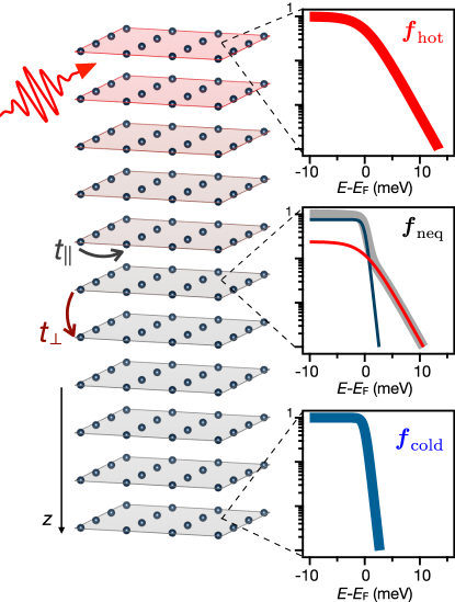
Figure 1: Setup. Cartoon of the layered correlated material impulsively excited on the top surface by ultrafast light pulses. We assume that the excitation drives a fast thermalization of the electronic population establishing an electronic temperature $T_{\mathrm{hot}}$ on the topmost layers of the sample. The right panels display the calculated transient electronic distributions at different depths. $f_{\mathrm{hot}}$ and $f_{\mathrm{cold}}$ are Fermi distribution functions at temperatures $T_{\mathrm{h}}$ and $T$ respectively. In the right-middle panel the non-equilibrium distribution is plotted in grey. In red and blue we report the ”hot” and ”cold” contributions to the non-equilibrium distribution function (see text). The transient temperature of the so-called ”cold” electrons can be different from the initial temperature $T_{c0}$ (see text).

II.1 The model

In order to identify the intrinsic role of electronic correlations, we model the LCM by a simple single-band layered Hubbard model. We do not include the interaction with phonons, which is however effective on longer timescales than the ones here addressed and does not significantly affect the present findings. The Hamiltonian reads:

$$H=\sum_{n=1}^{L}h_{n}+\sum_{n=1}^{L-1}\tau_{n,n+1}$$ (1)

with

$$h_{n}=\sum_{<i,j>\sigma}t_{\parallel}c^{\dagger}_{in\sigma}c^{\phantom{\dagger}}_{jn\sigma}+U\sum_{i}n_{in\uparrow}n_{in\downarrow}$$ (2)

and

$$\tau_{n,n+1}=\sum_{\sigma}t_{\perp}c^{\dagger}_{in\sigma}c^{\phantom{\dagger}}_{in+1\sigma}+h.c.$$ (3)

where $c^{\dagger}_{in\sigma}$ is a fermionic creation operator for an electron with spin $\sigma$ at the site $i$ belonging to the layer indexed by $n$, which ranges from 0 to $L$. $t_{\parallel}$ and $t_{\perp}$ represent, respectively, the intra- and inter-plane hopping amplitudes. The sum in the in-plane hopping term runs over pairs of nearest neighbouring sites and we introduce the number operator $n_{in\sigma}=c^{\dagger}_{in\sigma}c^{\phantom{\dagger}}_{in\sigma}$. We assume in-plane translational invariance so that we can introduce an in-plane momentum $\boldsymbol{k}=(k_{x},k_{y})$ and recast $h_{n}=\sum_{\boldsymbol{k}\sigma}\epsilon({\boldsymbol{k}})c^{\dagger}_{\boldsymbol{k}n\sigma}c^{\phantom{\dagger}}_{\boldsymbol{k}n\sigma}+U\sum_{i}n_{in\uparrow}n_{in\downarrow}$ with $\epsilon({\boldsymbol{k}})=-2t_{\parallel}(\cos(k_{x}a)+\cos(k_{y}a))$ and $a$ the lattice spacing. We fix the chemical potential in order to have an average occupation of one electron per site (half-filling) corresponding to the perfect particle-hole symmetric case. As a consequence, the total number of electrons per layer is conserved during the dynamics. This choice allows us to model energy transport in the absence of mass and charge transport.

We study the non-equilibrium dynamics in the frame of model (1) by means of a time-dependent variational approach based on the generalized Gutzwiller approximation for layered systems Fabrizio (2012); Mazza et al. (2015). This approach provides a versatile tool for describing, in a non-perturbative way, the dynamics in the Hubbard model which is governed by the interplay between the hopping terms $t_{\parallel},t_{\perp}$ and the local Coulomb interaction $U$.

Within this approach, the effect of the interaction is described in terms of the effective mass renormalization $m^{*}=m/Z$ which is controlled by the interaction $U$ through the quasiparticle weight $Z(U)$. In the non-interacting limit $Z(U=0)$=1, whereas at finite interaction $Z<1$ and decreases as a function of $U$. Eventually, for a critical interaction strength, $U_{c}$, the system undergoes a metal-to-insulator Mott transition, corresponding to a vanishing quasiparticle weight, i.e. $Z(U_{c})\rightarrow 0$. In this regime, quasiparticle excitations are completely suppressed and the dynamics becomes dominated by high-energy incoherent excitations at energies $\sim U$ Georges et al. (1996). In this work we focus on the thermal dynamics of hot quasi-particles in the correlated metal regime, where Z is finite but significantly smaller than one.

II.2 Non-equilibrium protocol

We investigate the thermal dynamics by considering the time evolution, regulated by the interacting Hamiltonian (1), of two electronic populations at different temperatures. To tackle this non-equilibrium problem we define the following protocol. We start from the solution of the equilibrium variational problem at zero temperature and set an electronic temperature on each layer by coupling each layer to an external reservoir of electrons with dispersion $\epsilon_{bath}(\boldsymbol{k})$ and non-zero temperature. In practice, this is achieved by considering an auxiliary master equation for the quasiparticles and performing a short-time evolution of the coupled system until equilibration is reached.

We first solve the finite temperature equilibration for the entire system at a base temperature that we will refer to as $T_{c0}$, where the subscript ”c” stands for ”cold” and ”0” indicates the instant preceding the impulsive excitation, and obtain the finite temperature occupation matrix elements, $\langle c^{\dagger}_{\boldsymbol{k}n\sigma}c^{\phantom{\dagger}}_{\boldsymbol{k}n^{\prime}\sigma}\rangle(T_{c0})$, and quasiparticle renormalizations, $Z$. We then repeat the finite temperature equilibration with an higher temperature $T_{h}>T_{c0}$ for a smaller subsystem of five layers. At time $t=0$ we switch off the coupling with the reservoirs and we let the system evolve starting from the condition

$$\langle c^{\dagger}_{\boldsymbol{k}n\sigma}c^{\phantom{\dagger}}_{\boldsymbol{k}n^{\prime}\sigma}\rangle(T_{h})~{}\quad \mathrm{for} \quad n,n^{\prime}=1,\ldots,5$$ (4)

$$\langle c^{\dagger}_{\boldsymbol{k}n\sigma}c^{\phantom{\dagger}}_{\boldsymbol{k}n^{\prime}\sigma}\rangle(T_{c0})~{}\quad \mathrm{for} \quad n,n^{\prime}=6,\ldots,L.$$ (5)

II.3 Observables

We study the thermal transport by tracking the time evolution of the energy density of the $n^{th}$ layer

$$E_{n}(t)\equiv\langle\Psi(t)|h_{n}+\tau_{n,n+1}|\Psi(t)\rangle$$ (6)

and the layer-dependent occupation numbers $f_{n}(\boldsymbol{k},t)$, defined as

$$f_{n}(\boldsymbol{k},t)\equiv\langle\Psi(t)|c^{\dagger}_{\boldsymbol{k}n\sigma}c^{\phantom{\dagger}}_{\boldsymbol{k}n\sigma}|\Psi(t)\rangle,$$ (7)

where in both equations $\left|\Psi(t)\right\rangle$ represents the time-evolved Gutzwiller wavefunction. The observables defined by Eqs. 6 and 7 are used to extract, respectively, the heat flux and the evolution of the local electronic temperature.

In order to obtain the layer- and time-dependent electronic temperatures, we need to transform the layer-dependent occupation numbers given by Eq. (7) into energy distribution functions by means of a proper variable substitution. We note that in the equilibrated initial state at time $t=0$ the occupation numbers reproduce Fermi-Dirac distribution functions, at the corresponding layer temperatures, expressed as a function of the bath dispersion. We therefore define the non-equilibrium energy distribution functions by adopting the bath dispersion relation and expressing the occupation numbers as a function of the energy $\epsilon_{bath}(\boldsymbol{k})$:

$$f_{\mathrm{neq}}^{(n)}(\epsilon,t)\equiv f_{n}(\epsilon_{bath}(\boldsymbol{k}),t)$$ (8)

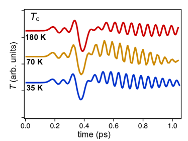
Figure S1: Temperature $T(t)$ of the quasi-equilibrium electronic distribution calculated at the 15^th layer for different values of the initial base temperature $T_{c}$=35 K (red), 70 K (yellow), 180 K (red).

In the rest of the paper we will measure temperatures by setting the bath dispersion equal to the bare electronic dispersion, i.e. $\epsilon_{bath}(\boldsymbol{k})=\epsilon(\boldsymbol{k})$. We mention here that a different choice would corresponds to a simple rescaling of the base temperature $T_{c0}$. In the supplemental (Fig. S1) we show that our results do not depend crucially on this choice.

Typical energy distribution functions are shown in Fig. 1 for a fixed instant of time at different depths of the layered system. We find that the non-equilibrium distribution function $f_{\mathrm{neq}}^{(n)}(\epsilon,t)$ can be fitted with a superposition of two equilibrium Fermi-Dirac distributions: i) a hot distribution at the temperature $T_{h}$, fixed by the initial perturbation, and of weight $\rho_{\mathrm{hot}}(n,t)$; ii) a cold distribution characterized by a time- and layer-dependent temperature $T(n,t)$ and of weight $1-\rho_{hot}(n,t)$. This decomposition can be written as:

$$f_{\mathrm{neq}}^{(n)}(\epsilon,t)=f_{\mathrm{hot}}\rho_{\mathrm{hot}}(n,t)+f_{\mathrm{cold}}\left[1-\rho_{\mathrm{hot}}(n,t)\right],$$ (9)

with $0\leq\rho_{\mathrm{hot}}(n,t)\leq 1$, $f_{\mathrm{hot}}=f(\epsilon,T_{h})$ and $f_{\mathrm{cold}}=f(\epsilon,T(n,t))$. Practically, for each fixed $n$ and $t$ values, we fitted $f_{\mathrm{neq}}^{(n)}(\epsilon,t)$, computed via Eq. 8, with the expression given by Eq. 9, $\rho_{\mathrm{hot}}(n,t)$ and $T(n,t)$ being the only two fitting parameters.

Eq. (9) is found to hold for any instant of time and layer index. This provides a clear physical interpretation of the transient propagation of energy and the definition of a local time-dependent electronic temperature. Initially, the perturbation creates a population of hot electrons described by $\rho_{\mathrm{hot}}(n,t)$ which propagates across the layers. Remarkably, while the temperature of the hot electrons is fixed at $T_{h}$, the temperature of the remaining $1-\rho_{\mathrm{hot}}(n,t)$ fraction of electrons in the ”cold” state $T(n,t)$ changes in time . We therefore identify $T(n,t)$ as the spatio-temporal evolution of the local electronic temperature which is determined by the interaction between the cold electrons on each layer and the hot electrons propagating through the system. We pinpoint that $T(n,t)$ (referred throughout the manuscript as the ”cold” electrons temperature) should not be confused with the initial system’s temperature $T_{c0}$.

The heat flux $q_{n}$ at layer $n$ and along the $z$-direction perpendicular to the planes is extracted by applying the continuity equation to the energy density (6)

$$\frac{\partial q_{n}}{\partial z}+\frac{\partial E_{n}}{\partial t}=0$$ (10)

where the discrete spatial derivative defined with respect to the interlayer distance $a$, $\frac{\partial q_{n}}{\partial z}=(q_{n+1}-q_{n})/a$.

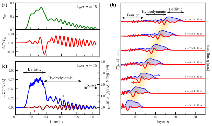
Figure 2: Sub-picosecond thermal dynamics. (a) Dynamics of the hot electron population (top) and relative temperature variation of the ”cold” electronic population (bottom) recorded on layer $n=15$. (b) Layer profiles of the temperature of the ”cold” electronic population (red, left axis) and of the heat flux (blue, right axis) at different instant of times. The blurred yellow band highlights the wave packet of temperature oscillations that follows the ballistic front. (c) Dynamics of the heat flux (blue, right axis) and temperature gradient of the ”cold” electronic population (red, left axis) on layer $n=15$. Arrows indicates the three regimes of thermal transport discussed in the main text.

III Ultrafast thermal dynamics

In this section we show how this model offers the possibility to access different regimes of non-conventional heat transport on the sub-picosecond timescale. Each regime will be then discussed and analysed in the following sections. We consider $t_{\perp}$=$t_{\parallel}=60~{}\mathrm{meV}$ and $U=0.65~{}\mathrm{eV}$, which correspond to an interaction-driven mass renormalization $m/m^{*}\simeq 0.3$, and a lattice spacing $a=5$ Å. As we shall see, this value of effective mass renormalization is consistent with experimental estimates for SrVO₃.

Initially the system is at the temperature $T_{c0}\simeq 35~{}\mathrm{K}$ and we create at time $t=0$ a non-equilibrium population of hot electrons on the first five layers corresponding to a hot temperature $T_{h}=10\times T_{c0}.$

Fig. 2a reports the results for the time evolution of the hot population weight and the local electronic relative temperature variation, $\Delta T/T_{c0}(n,t)$ with $\Delta T=T(n,t)-T_{c0}$, recorded on layer $n$=15, which we take as representative of the inner region of the slab. For times $0<t\lesssim 150~{}\mathrm{fs}$, both $\rho_{\mathrm{hot}}(15,t)$ and $T(15,t)$ remain fixed to the equilibrium values $\rho_{\mathrm{hot}}=0$ and $T=T_{c0}$. At $t\sim 150~{}\mathrm{fs}$ the perturbation reaches the $n=15$ layer and the dynamics that follows can be neatly divided in three steps.

i) In the time window $150-400~{}\mathrm{fs}$ the dynamics is characterized by a significant increase of $\rho_{\mathrm{hot}}(15,t)$ highlighting the arrival of the propagating hot electron population. On this time scale, the electronic relative temperature variation remains limited. This is indicative of a ballistic regime of energy transport in which the energy flows without inducing any heating in the underlying quasi-equilibrium distribution.

ii) For $t\gtrsim 400~{}\mathrm{fs}$ the hot electron population displays a sharp drop and, concomitantly, we observe the activation of a fast oscillatory dynamics in the electronic temperature of the cold electrons. Initially the oscillations are centered around a value higher than the initial equilibrium temperature $T_{c0}$ indicating that the transit of the ballistic front of hot electrons induced the heating of the population of cold electrons on the layer.

iii) Eventually the system equilibrates for $t\gtrsim 0.9~{}\mathrm{ps}$ with the residual damped temperature oscillations converging to $T_{c0}$.

We gain further insight into the thermal dynamics by comparing the dynamics of the local electronic temperature with the heat flux $q_{n}(t)$ at layer $n$. Panel (b) of Fig. 2 reports the spatial profiles of the heat flux (right axis, blue trace) and of the local electronic temperature (left axis, red trace) at fixed instants of time. The broad feature at the forefront of the heat flux profile indicates the propagation of a ballistic energy front accompanied by a small and more localized perturbation of the electronic temperature. At the back front of the ballistic heat flux, as indicated by the blurred yellow band in Fig. 2b, we observe the formation of a sharp sinusoidal feature in the spatial profile of the temperature. In the time domain, this sharp feature marks the separation between the first two dynamical regimes of the local temperature observed in panel (a) for the layer $n=15$. The presence of this pronounced oscillation of the temperature spatial profile is accompanied by weaker temperature oscillations with smaller spatial periodicity in the layers behind the ballistic front.

To fully characterize the thermal dynamics regimes occurring after the ballistic front has transited, we further compare the dynamics of the heat flux with that of the temperature gradient $\nabla_{\perp}T(t)=(T_{n+1}(t)-T_{n}(t))/a$ perpendicular to the layers. These quantities are shown in Fig. 2c for the $n$=15 layer. In the time window $0.15-0.4~{}\mathrm{ps}$, the ballistic regime shows up as a sharp increase of the heat flux with no sizeable effect on the temperature gradient. In correspondence of the end of the ballistic regime, i.e. the sharp drop of the heat current, an oscillatory dynamics is activated for the temperature gradient. The oscillatory dynamics of $\nabla_{\perp}T(t)$ is maintained in the 0.4-0.9 ps time window, along with a residual positive heat current on the layer. At $t\gtrsim~{}0.9$ ps the heat current displays damped oscillations centred around zero indicating the recovery of local thermal equilibrium. Remarkably, the equilibration is characterized by the synchronization between the dynamics of the temperature gradient and the heat flux. In this regime, we can define an instantaneous proportionality between the heat flux and temperature gradient, i.e. $q_{n}(t)\propto-\nabla_{\perp}T(t)$, indicating that the heat transfer process is well described by a Fourier-like heat transfer law.

At intermediate times ($0.4<t<0.9~{}\mathrm{ps}$), before Fourier-like transport sets in, there is a residual positive flow of the heat current with an oscillatory dynamics of $-\nabla_{\perp}T(t)$ that is not simply proportional to that of $q_{n}$($t$). This fact reveals the presence of a new heat transport regime which bridges the ballistic regime established at the arrival of the perturbation ($0.15<t<0.4~{}\mathrm{ps}$) and the Fourier-like transport setting in at long times after the perturbation has transited ($t>$0.9 ps). This intermediate regime is characterized by a residual population of hot electrons on the layer and by an oscillatory dynamics of the temperature of the cold electron population. We identify this regime as a hydrodynamic transport of heat sustained by the exchange of energy between the two sub-populations of hot and cold electrons. By comparing the dynamics on the single layer (Figs. 2a,c) with the layer profiles at different times (Fig. 2b), we can observe that the emergence of the hydrodynamic regime coincides with transit of the sharp sinusoidal feature in the spatial profile of the temperature at the trailing edge of the heat flux ballistic front. As it will be further discussed in the following sections, this feature can be considered as a temperature wave-packet propagating through the system.

Summarising, the sub-picosecond thermal dynamics of electrons displays three subsequent regimes of heat transport: i) the ballistic propagation of energy at the front of the perturbation; ii) the hydrodynamic regime at the trailing edge of the ballistic front. The former is characterized by a wave-like propagation of the electronic temperature; iii) a Fourier-like heat transport driving the recovery of thermal equilibrium. The time and space extension of the three regimes are indicated by the arrows in the plots of the dynamics at fixed layer index (see Fig. 2c) and of spatial profiles at fixed time (see Fig. 2b). In the remaining of the paper we analyse in detail the different regimes and discuss the possibility to control their onset in layered correlated materials.

IV Ballistic energy transport

In this section we will address the possibility of controlling the initial ballistic energy transport by tuning the microscopic parameters entering in the Hubbard model (1). In the ballistic regime, the energy is mostly carried by the population of hot electrons at temperature $T_{h}$. The energy propagates through hopping processes of the hot electrons excited in the first layers. Layered correlated materials thus offer two complementary ways to control the inter-layer coupling and, in turn, the velocity of propagation of the ballistic front, namely tuning either the anisotropy of the system, $t_{\perp}$/$t_{\parallel}$, or the strength of the interaction, $U$. The increase of the latter drives a reduction of the quasiparticle weight $Z$, which leads to a larger effective mass for the interlayer motion and a smaller effective hopping, $t_{\perp}^{*}=Zt_{\perp}$.

We show these effects in Fig 3 where we report the spatio-temporal dynamics of the hot electron population $\rho_{\mathrm{hot}}(n,t)$ obtained for different values of anisotropy (horizontal gray arrow) and relative interaction strength (vertical red arrow). Increasing either one the propagation velocity of the wavefront is diminished. In the inset we plot the velocity of ballistic propagation $v_{\mathrm{b}}$ as a function of $U$ for $t_{\perp}$/$t_{\parallel}$ = 1. $v_{\mathrm{b}}$ is defined as the slope of the white dashed line in Fig. 3. The correlation-induced renormalization of $t^{*}_{\perp}$ strongly suppresses the energy propagation along the $z$-direction.

For the sake of applications, we note that, in nanosystems with sizes of the order of the ballistic mean free path, the thermal conductivity becomes a size-dependent property Mingo and Broido (2005); Muñoz et al. (2010); Bae et al. (2013); Caddeo et al. (2017). Nanoengineering of LCM, combined with proper tuning of $U$ and $t_{\perp}$/$t_{\parallel}$, thus offers a new mean to control, on the picosecond timescale, the velocity of ballistic heat pulses and, therefore, the thermal conductivity of nanodevices.

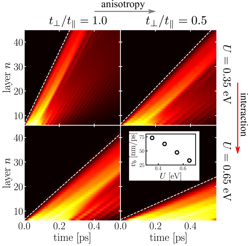
Figure 3: Control of ballistic energy propagation. The four panels matrix displays the ballistic dynamics of the hot-electron population for varying values of the correlation strength $U$ and anisotropy $t_{\perp}/t_{\parallel}$ ($t_{\parallel}$=60 meV). The color scale represents the amplitude of $\rho_{\mathrm{hot}}(n,t)$ (yellow: maximum; black: minimum). The inset displays the speed $v_{\mathrm{b}}$ of the ballistic wavefront (see dashed lines in the main panels) for different values of $U$ at $t_{\parallel}=t_{\perp}$.

V Hydrodynamic energy transport: emergent electronic temperature waves

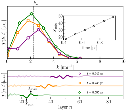
Figure 4: Spectral analysis in $k$-space of the electronic temperature waves. Top panel: spatial Fourier transform of the layer profile of the electronic temperature at three different times, $t=0.505~{}\mathrm{ps}$ (diamonds), $t=0.735~{}\mathrm{ps}$ (squares) and $t=0.945~{}\mathrm{ps}$ (circles). The inset shows the position of the minimum of the temperature oscillation, indicated in the bottom panel, as a function of time. The vertical dashed line indicated by $k_{*}$ shows the average of the position of the three peaks. Bottom panel: Portions of the temperature profiles at different times used to compute the discrete Fourier transform.

V.1 Temperature wave-packets

The results reported in Fig. 2 demonstrate that a purely electronic hydrodynamic transport regime can be achieved in our correlated system on much faster time scales than the more conventional phononic counterpart Beck et al. (1974); Lee et al. (2015); Huberman et al. (2019). Similarly to the phononic case, this hydrodynamic regime manifests itself by a wave-like propagation of temperature oscillations, which emerge after the ballistic front has transited (see arrows in Fig. 2c). In this section, we will quantitatively describe the characteristics of temperature wave-like propagation, as it emerges from our microscopic model.

In order to characterize this regime we track the position of the minimum of the wave packet $X_{\mathrm{min}}$ and we observe that it linearly increases in time (See the inset of Fig. 4a), allowing us to estimate the wave packet group velocity from the simple relation $X_{\mathrm{min}}=v_{g}t$. We obtain $v_{g}\sim 30~{}\mathrm{nm}/\mathrm{ps}$ of the same order of magnitude of the ballistic energy wavefront velocity. A similar result is obtained when tracking the time-dependent maximum of the wave-packet, $X_{\mathrm{max}}$. This result suggests that we can approximately describe the wave packet as a superposition of weakly-dispersive waves with frequencies $\nu_{k}=v_{g}k/2\pi$.

In order to identify the barycentric wavevector of the propagating wave packet, in the top panel of Fig.  4 we report the spatial Fourier transform of the electronic temperature profile in the spatial window where the propagating packet is present, as highlighted in the three curves of the bottom panel, which correspond to three different times, $t=0.505~{}\mathrm{ps}$, $t=0.735~{}\mathrm{ps}$ and $t=0.945~{}\mathrm{ps}$. The small number of layers included in the Fourier window produces spectrally broaden peaks with the maximum occurring at slightly different $k$ values for different times. We estimate the peak wavevector by taking the average of the three peaks observed at the three chosen times, obtaining $k_{*}\sim 2.2~{}\mathrm{nm^{-1}}$, corresponding to a wavelength $\lambda\sim 2.85~{}\mathrm{nm}$. Inserting this result in the linear dispersion relation we obtain a frequency $\nu_{*}\sim 10.5~{}\mathrm{THz}$. We notice that in the time domain, and at fixed layer index, this frequency corresponds to the inverse of the period of the large amplitude temperature oscillation originating after the transit of the ballistic energy wavefront, as shown in Fig. 2a.

V.2 Macroscopic model

We now compare the predictions of the microscopic model to a phenomenological model for the description of the hydrodynamic regime characterized by the emergence of electronic temperature waves. This approach recently proved effective in describing phononic temperature wave oscillations in graphite Gandolfi et al. (2019).

The phenomenological approach is based on the Dual Phase Lag Model (DPLM)Tzou (2014), which modifies Fourier law by introducing a causality relation between the onset of $\nabla_{\perp}T$ and the heat flux

$$q\left(t+\tau_{q},z\right)=-\kappa_{T,el}\ \nabla_{\perp}T\left(t+\tau_{T},z\right).$$ (11)

In other words, the DPLM introduces a delay between the time at which the temperature gradient $\nabla_{\perp}T$ is established, $t+\tau_{T}$, and the time when the interlayer heat flux $q$ sets in, $t+\tau_{q}$. The expansion of Eq. 11 to first order, and its combination with the local conservation of energy at time $t$, gives rise to a second order parabolic differential equation for the temperature variation $\Delta T(t,z)$=$T(t,z)-T_{\mathrm{c0}}$.

We look for wave-like solutions of this differential equation starting from a temperature pulse triggered at initial time on the top side of the sample slab. Following Ref. 18, the pulse can be described by a superposition of plane-waves of real-valued wave vectors $k$ and complex frequencies $\nu$. Underdamped plane-wave solutions for $\Delta T(t,z)$ are found if the condition $\tau_{q}>2\tau_{T}$ is met. These temperature waves are characterized by the complex-valued dispersion relation

$$\nu(k,R,\alpha)=\nu_{1}(k,R,\alpha)+\mathrm{i}\nu_{2}(k,R,\alpha),$$ (12)

where $\nu_{1,2}(k,R,\alpha)$ depend on the wavevector $k$, and on the parameters $R=\frac{\tau_{T}}{\tau_{q}}$ and thermal diffusivity $\alpha=\frac{\kappa_{T,el}}{C_{el}}$, $\kappa_{T,el}$ and $C_{el}$ being the electronic thermal conductivity and specific heat, respectively.

The analytic expressions for the real-valued $\nu_{1}$ and $\nu_{2}$, together with the quality factor defined as $Q(k,R,\alpha)=\frac{\nu_{1}}{\nu_{2}}$, are reported in Supplementary Information. In principle, the quantities $R$ and $\alpha$ do depend on the electronic temperature $T$. However, since the relative variation $|\Delta T(t)|/T_{c0}\ll 1$ (see Fig. 2a), the temperature dependence may be taken with respect to the initial base temperature $T_{c0}$, i.e. $R$=$R$($T_{c0}$) and $\alpha$=$\alpha$($T_{c0}).$

In order to reveal under which conditions temperature waves are sustained, we exploit the dispersion $\nu_{1}$($k$) and its quality factor $Q$, upon insertion of the microscopic parameters relevant for SrVO₃ as extracted both from solution of the Hubbard model (previous sections) and supplemented by parameters derived from the literature. We first determine the quantities $R$ and $\alpha$. We identify the time for setting a variation in the temperature gradient, $\tau_{T}$, as the electronic thermalization time. The local thermalization time in SVO is estimated to be as short as $\sim$5 fs on the basis of angle-resolved photoemission spectroscopy Aizaki et al. (2012) and optical conductivity Zhang et al. (2015) data (see Supplementary Information). We thus set $\tau_{T}$=5 fs. This time scale is compatible with the attribution of an instantaneous local temperature on the sub-picosecond time scale, as assumed in the previous sections. On the other hand, the heat flux dynamics in Fig. 2c shows that the synchronization between $\nabla_{\perp}T$ and $q$ starts at $\sim 900~{}\mathrm{fs}$, i.e. $500~{}\mathrm{fs}$ after the ballistic wavefront has transited through the 15^th layer. We can thus assume $\tau_{q}\simeq$500 fs. Based on these assumptions, we obtain $R=\tau_{T}/\tau_{q}\sim 0.01$ which is well below the threshold $R<0.5$ for the observation of a wavelike behaviour. While the electronic scattering time is expected to weakly depend on the temperature, the temperature dependence of $\tau_{q}$ is tested by calculating the solution of the single-band Hubbard model at different base temperatures $T_{c0}$. As shown in Fig. S1, the results demonstrate that $\tau_{q}$ is almost independent of $T_{c0}$, thus allowing to assume a temperature independent value of $R$. The temperature dependence of the wave frequencies is instead retained through $\alpha$. Specifically, for the case of SVO, $C_{el}$=$\gamma T$ with $\gamma$=2.4$\times 10^{2}~{}\mathrm{Jm}^{-3}\mathrm{K}^{-2}$ Inoue et al. (1998). As for $\kappa_{T,el}$($T$) we retrieve it from the temperature dependent electrical conductivity, $\sigma(T)$, of SVO single crystals Inoue et al. (1998) upon application of the Wiedemann-Franz-Lorentz relation: $\kappa_{T,el}$=$L\sigma T$, $L$=2.44$\cdot$10^-8 W$\Omega$K^-2 being the Lorentz number. The temperature-dependent $\kappa_{T,el}$ ranges from $\simeq$10 Wm^-1K^-1 at 300 K to $\simeq$20 Wm^-1K^-1 at 35 K.

With this parameters at hand, in Fig. 5 we show the dispersion relation for the temperature oscillation frequency $\nu_{1}$ (top panel) and the corresponding $Q-$factor (bottom panel) as a function of wavelength $\lambda=2\pi/k$ and base temperature $T_{c0}$. The temperature wave frequency $\nu_{*}\sim 10.5~{}\mathrm{THz}$, obtained from the microscopic model at the base temperature $T_{c0}=35$ K, falls within the range of the allowed frequencies and is compatible with two possible wavelengths, $\lambda\sim 6.5~{}\mathrm{nm}$ and $\lambda\sim 1.1~{}\mathrm{nm}$. These wavelengths correspond to $Q-$factors $\sim$ 5 and 0.2, respectively, therefore only the longest wavelength is expected to be detectable. This wavelength falls pretty close to the estimate $\lambda\sim 2.85~{}\mathrm{nm}$ obtained from the microscopic single-band Hubbard model.

Given the quite general assumptions on the parameters of the microscopic model and the realistic values used in the phenomenological model, the above comparison shows an overall good agreement between the temperature waves dynamics obtained from the sub-picoseconds dynamics of the single-band Hubbard model and the predictions based on a macroscopic model. Such an agreement further confirms that LCM can sustain, in the hydrodynamic regime, temperature waves with wavelengths and periods fully compatible with state-of-the-art materials growth techniques and time-resolved spectroscopies. More in general, the frequencies and $Q$-factor values reported in Fig. 5 show that the manifestation of temperature waves in LCM can be observed up to temperatures as high as $300~{}\mathrm{K}$. This is the consequence of the fact that the energy scales controlling the electronic dynamics, i.e. $t_{\parallel}$=$t_{\perp}$=60 meV and $U$=650 meV, correspond to temperatures of $\simeq$ 700 K and $\simeq$ 7000 K respectively. At variance with the phononic case, the sub-picosecond electronic hydrodynamic regime is thus expected to be very robust against temperature, giving rise to the emergence of temperature wave-like oscillations in real materials at ambient conditions.

V.3 Control of temperature waves in the hydrodynamic regime

We end this section by discussing how, similarly to the ballistic transport regime, the electronic interactions are key to control the wave-like temperature propagation. In Fig. 6 we report the temperature dynamics at layer $n=15$ for different values of the interaction $U$. We observe that the smaller the interaction the smaller is the temperature oscillation amplitude triggered in the population of cold electrons by the transit of the hot electron wavefront. The data further show that the temperature oscillation periods, indicated in Fig. 6 by the black arrows, decrease as the interaction $U$ is decreased. In general, the thermal dynamics of quasiparticles become slower as the interaction is increased, a fact also observed for the case of the ballistic energy propagation. This may be traced back to the effect of the correlation-driven renormalization of the quasi-particle effective mass. Wrapping up, tuning the electronic correlations strength, which controls the quasiparticle effective mass renormalization, can act as a control parameter for the frequency and amplitude of transient temperature waves in LCM.

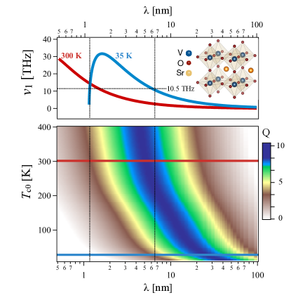
Figure 5: Temperature wave dispersion in SVO₃. Top panel: electronic temperature oscillation frequency, $\nu$=$\omega_{1}/2\pi$, vs oscillation’s wavelength, $\lambda$, at a base temperatures $T_{c0}$=35 K (blue line) and 300 K (red line). Bottom panel: quality factor (colormap) vs oscillation’s wavelength, $\lambda$, and base temperature $T_{c0}$. Calculations based on Ref. Gandolfi et al. (2019) upon insertion of input parameters from experiments, $\alpha$ and $\tau_{T}$, and from non-equilibrium thermal dynamics results from the layered Hubbard model (see text), $\tau_{q}$. In both panels a linear-log plot is adopted.

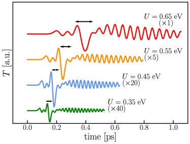
Figure 6: Control of temperature wave-like oscillations. Temperature $T(t)$ of the ”cold” electronic oscillation at the $n=15$ layer for different values of $U$ (the same values used in the inset of Fig. 3) Some of the data have been magnified and the curves shifted for graphical reasons. The horizontal arrows highlight the oscillation periods that match the frequency $\nu_{*}$ extracted from spectral analysis of the temperature wave packet.

VI Recovery of Fourier-like heat transport

After the transit of the ballistic heat wavefront and of the temperature wave-packet, the hydrodynamic regime gradually evolves into a more conventional dynamics ($t>$0.9 ps in Fig. 2). Here, the non-equilibrium hot electron population has already left the region of interest, giving rise to a free oscillatory equilibration dynamics of the temperature of ”cold” electrons. The wavelength of the temperature oscillation is smaller than that of the temperature wavepacket propagating with speed $v_{g}$ (hydrodynamic regime), as may be seen in Fig. 2(b). In the present regime, the oscillation frequency (see Fig. 2(c)) exactly matches 4$t^{*}_{\perp}/h$, which is the renormalized bandwidth in the direction perpendicular to the layers (Figure 1). The heat flux left behind by the temperature wavepacket freely oscillates with a frequency controlled by $t^{*}_{\perp}$, which is the only intrinsic energy scale of the Hubbard Hamiltonian playing a role on the hundreds femtoseconds timescale. The oscillating $q_{n}$($t$) thus acts as the source for the temperature gradient, which instantaneously follows the temperature variation, i.e. without any delay, as expressed in Fourier law $q\left(t,z\right)=-\kappa_{T,el}\ \nabla_{\perp}T\left(t,z\right)$. For instance, for $U=0.65~{}\mathrm{eV}$ one has $t^{*}_{\perp}\simeq 0.33t_{\perp}$=20 meV and the oscillation periods reads $h/4t^{*}_{\perp}\simeq$ 50 fs.

Interestingly, we can estimate the electronic thermal conductivity by evaluating the ratio between the oscillation amplitude of the heat flux and that of the temperature gradient, i.e. $\kappa_{T,el}$=$\left\lVert q\right\rVert/\left\lVert\nabla_{\perp}T\right\rVert$ where the symbol $\left\lVert...\right\rVert$ represents the oscillation amplitude. As an example of the moderately interacting regime we consider $U=0.45~{}\mathrm{eV}$, resulting in $\frac{U}{U_{c}}\sim$0.55, that is quite far from the Mott transition critical point, $U/U_{c}\sim$1. In doing so we estimate $\kappa_{T,el}\simeq$440 Wm^-1K^-1, which is in the order of typical zero-frequency electronic thermal conductivity of conventional metals. On the other hand, when we increase $U$, the interactions drive a larger temperature gradient (see Fig. S2) which in turn results in a very small value of $\kappa_{T,el}$ Karrasch et al. (2016). For instance, when $U/U_{c}$=0.7-0.8, the estimated thermal conductivity is in the range 40-2.5 Wm^-1K^-1, a value of the same order of the zero-frequency conductivity reported for SVO (Inoue et al., 1998). Thus, despite its simplicity, the layered Hubbard model predicts the correct order of magnitude of Fourier-like thermal conductivity of materials for a very wide range of correlation strengths.

VII Conclusions

In conclusion, we have proposed layered correlated materials as a platform enabling to access a rich variety of heat transport regimes. We consider a paradigmatic layered Hubbard model in equilibrium at a given temperature and we impulsively heat one side of the system. The transient dynamics undergoes, on ultrashort space and timescales, a crossover between ballistic energy transport and electronic temperature wave-like oscillations in the hydrodynamic regime. Eventually, the Fourier-like heat transport regime is recovered on the picosecond time-scale. Specifically, transition metal oxides thin films and heterostructures, with typical thicknesses and periodicities in the few nanometers range, are here predicted to sustain electronic temperature wave-like oscillations in a parameter space fully compatible with state-of-the-art time resolved calorimetry techniques Giannetti et al. (2016). The temperature oscillation frequency can be tuned via the correlation strength and is predicted to persist up to room temperature.

The outreach of our results ranges beyond LCM. Among the most interesting applications we foresee is nanoengineering of superlattices made out of correlated materials, allowing for coherent control of temperature waves in nanodevices. For instance, LCM can be grown in heterostructures with control of the physical properties at the level of single atomic layers Hwang et al. (2012) and with the possibility of engineering artificial periodicities to select high-$Q$ modes of temperature waves. The recent introduction of the temperonic crystal Gandolfi et al. (2020), i.e. a periodically modulated structure which behaves like a crystal for temperature waves, provides a new tool to coherently control temperature pulses in correlated heterostructures. Furthermore, strong correlations, and their control via the interlayer twist angle, have recently been reported in graphene superlattices Cao et al. (2018); Seyler et al. (2019); Lu et al. (2019). The present work paves the way to the control of electronic ballistic propagation and to the engineering of nanodevices exploiting the wavelike nature of the electronic heat transfer on the sub-picosecond timescale.

VIII Acknowledgments

G.M. acknowledges financial support from the Swiss National Science Foundation through an AMBIZIONE grant. Part of this work has been supported from the European Research Council (ERC-319286-QMAC). M.G. acknowledges financial support from the CNR Joint Laboratories program 2019-2021. F.B. acknowledges financial support from Université de Lyon in the frame of the IDEXLYON Project -Programme Investissements d’ Avenir (ANR-16-IDEX-0005) and from Université Claude Bernard Lyon 1 through the BQR Accueil EC 2019 grant. M.G and F.B acknowledge financial support from the MIUR Futuro in ricerca 2013 Grant in the frame of the ULTRANANO Project (project number: RBFR13NEA4). C.G acknowledge support from Università Cattolica del Sacro Cuore through D.2.2 and D.3.1 grants. M.C. and C.G. acknowledge financial support from MIUR through the PRIN 2015 (Prot 2015C5SEJJ001) and PRIN 2017 (Prot. 20172H2SC4$\_$005) programs.

Supplementary Information for Thermal dynamics and electronic temperature waves in layered correlated materials

Supplementary figures

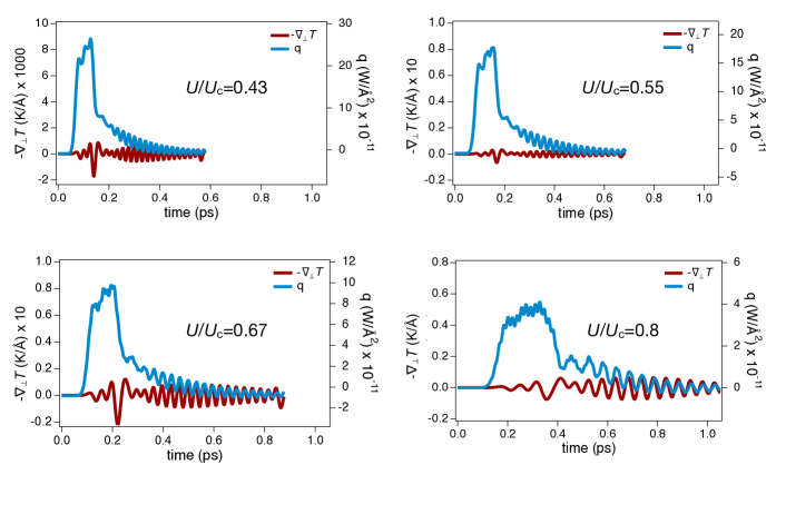
Figure S2: Dynamics of the interlayer temperature gradient -$\nabla_{\perp}T(t)$ (purple line) and heat flux $q(t)$ (blue line) at the 15^th layer for different values of $U/U_{c}$. The data reported in the figure have been used to retrieve the electronic thermal conductivity in the Fourier-like regime.

Allowed frequencies and wavevectors

As discussed in Ref. 18, the wave equation for the temperature variation $\Delta T(t,z)$=$T(t,z)$-$T_{\mathrm{c0}}$ is derived from the combination of Eq. 9 and the local energy conservation. A wave-like behaviour of $\Delta T(x,t)$ emerges Gandolfi et al. (2019) when the wavevector $k$ falls in the range $k_{lo}<k<k_{hi}$ with

$${k_{lo(hi)}=\sqrt{\frac{2}{\alpha\tau_{T}}\left(\frac{\tau_{q}}{\tau_{T}}\right)\left(1-\frac{1}{2}\frac{\tau_{T}}{\tau_{q}}-(+)\sqrt{1-\frac{\tau_{T}}{\tau_{q}}}\ \right)}}$$ (S1)

yielding real and imaginary frequency components:

$$\omega_{1}=\mp\sqrt{-\left[\frac{\alpha^{2}}{4}\left(\frac{\tau_{T}}{\tau_{q}}\right)^{2}k^{4}+\frac{\alpha}{\tau_{q}}\left[{1\over 2}\left(\frac{\tau_{T}}{\tau_{q}}\right)-1\right]k^{2}+\frac{1}{4\tau_{q}^{2}}\right]}$$ (S2)

$$\omega_{2}=\left[\frac{1}{2\tau_{q}}+\frac{\alpha}{2}\left(\frac{\tau_{T}}{\tau_{q}}\right)k^{2}\right]$$ (S3)

The $Q$-factor is easily calculated as $Q$=$|\omega_{1}|/\omega_{2}$

Scattering time in SVO from optical data

The electronic scattering rate can be extracted from optical spectroscopy data. For strongly interacting electrons, the interactions strongly affects the scattering rate and give rise to a frequency dependent scattering rate, which is accounted for by the extended Drude model. The inverse scattering is directly related to the Drude dielectric function through the relation:

$$\frac{1}{\tau(\omega)}=-\frac{\omega^{2}_{p}}{\omega}\mathrm{Im}\frac{1}{\epsilon_{D}(\omega)-\epsilon_{\infty}}$$ (S4)

$\omega_{p}$ being the undressed plasma frequency and $\epsilon_{\infty}$ the effective permittivity that accounts for the interband transitions involving electronic states in the valence and other bands. In Fig. S3 we report the optical scattering rate extracted from the optical data reported in Ref. 37. Considering the density of carriers in SVO, $n$=1.76$\cdot$10²² cm^?3, we obtain $\omega_{p}$=4.6 eV, which corresponds to the plasma frequency obtained from the fitting with a Drude model. The calculated $\tau(\omega)$ shows a pronounced decrease in the range 0.1-0.6 eV, which is connected to the strong scattering with modes at very high frequency, in agreeement with the photoemission data discussed in the next session. A value $\tau\approx$2 fs is reached at $\omega>$0.6 eV, whereas the low-frequency limit is $\tau\approx$5 fs. If we consider a pump-probe experiment, which represents a promising configuration to observe wave-like temperature oscillations, it is natural to assume that the high-energy ($>$0.6 eV) excitations, directly photoinjected by the pump pulse (usually in the near-infrared or visible), scatter with high-energy modes within $\approx$1 fs. The low-energy electrons generated during this fast relaxation stage experience a progressively slower scattering time, which reaches a constant value of $\approx$5 fs at energies smaller than 0.1 eV (see Fig. S3). Since thermalization is related to the low-energy carriers, we can assume that the typical thermalization time is $\tau_{T}\approx$5 fs.

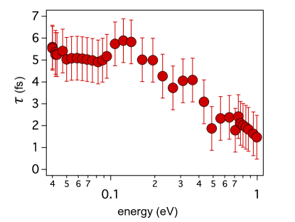
Figure S3: Optical scattering time of the conduction electrons for SVO, as extracted from the optical spectroscopy data reported in Ref. Zhang et al. (2015) by using Eq. S4.

Scattering time in SVO from photoemission

In order to evaluate the local thermalization time we can also refer to the SVO band structure, as measured by angle-resolved photoemission spectroscopy Aizaki et al. (2012). The electronic correlations manifest themselves in a high-energy contribution to the electronic self-energy, which exhibits a broad kink at $\hbar\Omega_{k}\sim$0.3 eV. We can thus assume that the typical timescale of electron-electron interactions is 1/$\hbar\Omega_{k}\sim$2 fs, which is perfect agreement with the high-energy scattering rate extracted from optical data, as discussed in the previous section.

References

- Chen (2005) Gang Chen, Nanoscale energy transport and conversion (Oxford University Press, 2005).
- Volz et al. (2016) Sebastian Volz, Jose Ordonez-Miranda, Andrey Shchepetov, Mika Prunnila, Jouni Ahopelto, Thomas Pezeril, Gwenaelle Vaudel, Vitaly Gusev, Pascal Ruello, Eva M Weig, et al., “Nanophononics: state of the art and perspectives,” The European Physical Journal B 89, 15 (2016).
- Li et al. (2012) Nianbei Li, Jie Ren, Lei Wang, Gang Zhang, Peter Hänggi, and Baowen Li, “Colloquium: Phononics: Manipulating heat flow with electronic analogs and beyond,” Rev. Mod. Phys. 84, 1045–1066 (2012).
- Luo and Chen (2013) Tengfei Luo and Gang Chen, “Nanoscale heat transfer - from computation to experiment,” Phys. Chem. Chem. Phys. 15, 3389–3412 (2013).
- Cahill et al. (2014) David G Cahill, Paul V Braun, Gang Chen, David R Clarke, Shanhui Fan, Kenneth E Goodson, Pawel Keblinski, William P King, Gerald D Mahan, Arun Majumdar, et al., “Nanoscale thermal transport. ii. 2003–2012,” Appl. Phys. Rev. 1, 011305 (2014).
- Siemens et al. (2010) Mark E. Siemens, Qing Li, Ronggui Yang, Keith A. Nelson, Erik H. Anderson, Margaret M. Murnane, and Henry C. Kapteyn, “Quasi-ballistic thermal transport from nanoscale interfaces observed using ultrafast coherent soft x-ray beams,” Nat. Mater. 9, 26 (2010).
- Minnich et al. (2011) J. Minnich, J. A. Johnson, A. J. Schmidt, K. Esfarjani, M. S. Dresselhaus, K. A. Nelson, and G. Chen, “Thermal conductivity spectroscopy technique to measure phonon mean free paths,” Phys. Rev. Lett. 107, 095901 (2011).
- Johnson et al. (2013) Jeremy A. Johnson, A. A. Maznev, John Cuffe, Jeffrey K. Eliason, Austin J. Minnich, Timothy Kehoe, Clivia M. Sotomayor Torres, Gang Chen, and Keith A. Nelson, “Direct measurement of room-temperature nondiffusive thermal transport over micron distances in a silicon membrane,” Phys. Rev. Lett. 110, 025901 (2013).
- Hoogeboom-Pot et al. (2015) Kathleen M. Hoogeboom-Pot, Jorge N. Hernandez-Charpak, Xiaokun Gu, Travis D. Frazer, Erik H. Anderson, Weilun Chao, Roger W. Falcone, Ronggui Yang, Margaret M. Murnane, Henry C. Kapteyn, and Damiano Nardi, “A new regime of nanoscale thermal transport: Collective diffusion increases dissipation efficiency,” Proc. Natl. Acad. Sci. USA 112, 4846 (2015).
- Chen et al. (2018) Xiangwen Chen, Chengyun Hua, Hang Zhang, Navaneetha K. Ravichandran, and Austin J. Minnich, “Quasiballistic thermal transport from nanoscale heaters and the role of the spatial frequency,” Phys. Rev. Applied 10, 054068 (2018).
- Frazer et al. (2019) Travis D. Frazer, Joshua L. Knobloch, Kathleen M. Hoogeboom-Pot, Damiano Nardi, Weilun Chao, Roger W. Falcone, Margaret M. Murnane, Henry C. Kapteyn, and Jorge N. Hernandez-Charpak, “Engineering nanoscale thermal transport: Size- and spacing-dependent cooling of nanostructures,” Phys. Rev. Applied 11, 024042 (2019).
- Guyer and Krumhansl (1966) R. A. Guyer and J. A. Krumhansl, “Thermal conductivity, second sound, and phonon hydrodynamic phenomena in nonmetallic crystals,” Phys. Rev. 148, 778–788 (1966).
- Beck et al. (1974) H. Beck, P.F. Meier, and A. Thellun, “Phonon hydrodynamics in solids,” Phys. Stat. Sol. (a) 24, 11–63 (1974).
- Lee et al. (2015) Sangyeop Lee, David Broido, Keivan Esfarjani, and Gang Chen, “Hydrodynamic phonon transport in suspended graphene,” Nature Communications 6, 6290 (2015).
- Ding et al. (2018) Zhiwei Ding, Jiawei Zhou, Bai Song, Vazrik Chiloyan, Mingda Li, Te-Huan Liu, and Gang Chen, “Phonon hydrodynamic heat conduction and knudsen minimum in graphite,” Nano Letters 18, 638–649 (2018).
- Cepellotti et al. (2015) Andrea Cepellotti, Giorgia Fugallo, Lorenzo Paulatto, Michele Lazzeri, Francesco Mauri, and Nicola Marzari, “Phonon hydrodynamics in two-dimensional materials,” Nature communications 6, 1–7 (2015).
- Li and Lee (2019) Xun Li and Sangyeop Lee, “Crossover of ballistic, hydrodynamic, and diffusive phonon transport in suspended graphene,” Phys. Rev. B 99, 085202 (2019).
- Gandolfi et al. (2019) Marco Gandolfi, Giulio Benetti, Christ Glorieux, Claudio Giannetti, and Francesco Banfi, “Accessing temperature waves: a dispersion relation perspective,” International Journal of Heat and Mass Transfer 143, 118553 (2019).
- Huberman et al. (2019) S. Huberman, R.A. Duncan, K. Chen, B. Song, V. Chiloyan, Z. Ding, A.A. Maznev, G. Chen, and K.A. Nelson, “Observation of second sound in graphite at temperatures above 100 K,” Science 364, 375 (2019).
- Zhang et al. (2020) Yingchao Zhang, Xun Shi, Wenjing You, Zhensheng Tao, Yigui Zhong, Fairoja Cheenicode Kabeer, Pablo Maldonado, Peter M. Oppeneer, Michael Bauer, Kai Rossnagel, Henry Kapteyn, and Margaret Murnane, “Coherent modulation of the electron temperature and electron–phonon couplings in a 2D material,” Proceedings of the National Academy of Sciences 117, 8788–8793 (2020).
- Gandolfi et al. (2020) Marco Gandolfi, Claudio Giannetti, and Francesco Banfi, “Temperonic crystal: A superlattice for temperature waves in graphene,” Phys. Rev. Lett. 125, 265901 (2020).
- Cepellotti and Marzari (2017) Andrea Cepellotti and Nicola Marzari, “Transport waves as crystal excitations,” Phys. Rev. Materials 1, 045406 (2017).
- Torres et al. (2019) Pol Torres, Francesc Xavier Alvarez, Xavier Cartoixà, and Riccardo Rurali, “Thermal conductivity and phonon hydrodynamics in transition metal dichalcogenides from first-principles,” 2D Materials 6, 035002 (2019).
- Machida et al. (2020) Yo Machida, Nayuta Matsumoto, Takayuki Isono, and Kamran Behnia, “Phonon hydrodynamics and ultrahigh–room-temperature thermal conductivity in thin graphite,” Science 367, 309–312 (2020).
- Simoncelli et al. (2020) Michele Simoncelli, Nicola Marzari, and Andrea Cepellotti, “Generalization of Fourier’s Law into Viscous Heat Equations,” Phys. Rev. X 10, 011019 (2020).
- Gandolfi et al. (2017) Marco Gandolfi, Luca Giuseppe Celardo, Fausto Borgonovi, Gabriele Ferrini, Adolfo Avella, Francesco Banfi, and Claudio Giannetti, “Emergent ultrafast phenomena in correlated oxides and heterostructures,” Phys. Scripta 92, 034004 (2017).
- Hartnoll (2015) Sean A Hartnoll, “Theory of universal incoherent metallic transport,” Nature Physics 11, 54–61 (2015).
- Lee et al. (2017) Sangwook Lee, Kedar Hippalgaonkar, Fan Yang, Jiawang Hong, Changhyun Ko, Joonki Suh, Kai Liu, Kevin Wang, Jeffrey J. Urban, Xiang Zhang, Chris Dames, Sean A. Hartnoll, Olivier Delaire, and Junqiao Wu, “Anomalously low electronic thermal conductivity in metallic vanadium dioxide,” Science 355, 371–374 (2017).
- Tokura et al. (2017) Yoshinori Tokura, Masashi Kawasaki, and Naoto Nagaosa, “Emergent functions of quantum materials,” Nature Physics 13, 1056–1068 (2017).
- Basov et al. (2017) D N Basov, N D Averitt, and D Hsieh, “Towards properties on demand in quantum materials,” Nat. Mat. 16, 1077–1088 (2017).
- Ordonez-Miranda et al. (2018) Jose Ordonez-Miranda, Younès Ezzahri, Karl Joulain, Jérémie Drevillon, and J. J. Alvarado-Gil, “Modeling of the electrical conductivity, thermal conductivity, and specific heat capacity of ,” Phys. Rev. B 98, 075144 (2018).
- Cesarini et al. (2019) Gianmario Cesarini, Grigore Leahu, Alessandro Belardini, Marco Centini, Roberto Li Voti, and Concita Sibilia, “Quantitative evaluation of emission properties and thermal hysteresis in the mid-infrared for a single thin film of vanadium dioxide on a silicon substrate,” International Journal of Thermal Sciences 146, 106061 (2019).
- Ben-Abdallah and Biehs (2014) Philippe Ben-Abdallah and Svend-Age Biehs, “Near-field thermal transistor,” Phys. Rev. Lett. 112, 044301 (2014).
- Ordonez-Miranda et al. (2019) Jose Ordonez-Miranda, Younès Ezzahri, Jose A. Tiburcio-Moreno, Karl Joulain, and Jérémie Drevillon, “Radiative thermal memristor,” Phys. Rev. Lett. 123, 025901 (2019).
- Moyer et al. (2013) Jarrett A. Moyer, Craig Eaton, and Roman Engel-Herbert, “Highly conductive srvo3 as a bottom electrode for functional perovskite oxides,” Advanced Materials 25, 3578–3582 (2013).
- Zhong et al. (2015) Zhicheng Zhong, Markus Wallerberger, Jan M. Tomczak, Ciro Taranto, Nicolaus Parragh, Alessandro Toschi, Giorgio Sangiovanni, and Karsten Held, “Electronics with Correlated Oxides: as a Mott Transistor,” Phys. Rev. Lett. 114, 246401 (2015).
- Zhang et al. (2015) Lei Zhang, Yuanjun Zhou, Lu Guo, Weiwei Zhao, Anna Barnes, Hai-Tian Zhang, Craig Eaton, Yuanxia Zheng, Matthew Brahlek, Hamna F. Haneef, Nikolas J. Podraza, Moses H. W. Chan, Venkatraman Gopalan, Karin M. Rabe, and Roman Engel-Herbert, “Correlated metals as transparent conductors,” Nature Materials 15, 204–210 (2015).
- Fabrizio (2012) Michele Fabrizio, “The out-of-equilibrium time-dependent gutzwiller approximation,” NATO Science for Peace and Security Series B: Physics and Biophysics (2012), 10.1007/978-94-007-4984-916.
- Mazza et al. (2015) G. Mazza, A. Amaricci, M. Capone, and M. Fabrizio, “Electronic transport and dynamics in correlated heterostructures,” Phys. Rev. B 91, 195124 (2015).
- Georges et al. (1996) Antoine Georges, Gabriel Kotliar, Werner Krauth, and Marcelo J. Rozenberg, “Dynamical mean-field theory of strongly correlated fermion systems and the limit of infinite dimensions,” Rev. Mod. Phys. 68, 13–125 (1996).
- Note (1) This result is confirmed using different fitting procedures in which is either considered a fixed parameter or fitting parameter.
- Mingo and Broido (2005) N. Mingo and D. A. Broido, “Carbon nanotube ballistic thermal conductance and its limits,” Phys. Rev. Lett. 95, 096105 (2005).
- Muñoz et al. (2010) Enrique Muñoz, Jianxin Lu, and Boris I Yakobson, “Ballistic Thermal Conductance of Graphene Ribbons,” Nano Letters 10, 1652–1656 (2010).
- Bae et al. (2013) Myung-Ho Bae, Zuanyi Li, Zlatan Aksamija, Pierre N Martin, Feng Xiong, Zhun-Yong Ong, Irena Knezevic, and Eric Pop, “Ballistic to diffusive crossover of heat flow in graphene ribbons,” Nature Communications 4, 1734 (2013).
- Caddeo et al. (2017) Claudia Caddeo, Claudio Melis, Andrea Ronchi, Claudio Giannetti, Gabriele Ferrini, Riccardo Rurali, Luciano Colombo, and Francesco Banfi, “Thermal boundary resistance from transient nanocalorimetry: A multiscale modeling approach,” Phys. Rev. B 95, 085306 (2017).
- Tzou (2014) Da Yu Tzou, Macro-to microscale heat transfer: the lagging behavior (John Wiley & Sons, 2014).
- Aizaki et al. (2012) S. Aizaki, T. Yoshida, K. Yoshimatsu, M. Takizawa, M. Minohara, S. Ideta, A. Fujimori, K. Gupta, P. Mahadevan, K. Horiba, H. Kumigashira, and M. Oshima, “Self-Energy on the Low- to High-Energy Electronic Structure of Correlated Metal ,” Phys. Rev. Lett. 109, 056401 (2012).
- Inoue et al. (1998) I. H. Inoue, O. Goto, H. Makino, N. E. Hussey, and M. Ishikawa, “Bandwidth control in a perovskite-type -correlated metal I. Evolution of the electronic properties and effective mass,” Phys. Rev. B 58, 4372–4383 (1998).
- Karrasch et al. (2016) C. Karrasch, D. M. Kennes, and F. Heidrich-Meisner, “Thermal Conductivity of the One-Dimensional Fermi-Hubbard Model,” Phys. Rev. Lett. 117, 116401 (2016).
- Giannetti et al. (2016) C. Giannetti, M. Capone, D. Fausti, M. Fabrizio, F. Parmigiani, and D. Mihailovic, “Ultrafast optical spectroscopy of strongly correlated materials and high-temperature superconductors: a non-equilibrium approach,” Adv. Phys. 65, 58 (2016).
- Hwang et al. (2012) H. Y. Hwang, Y. Iwasa, M. Kawasaki, B. Keimer, N. Nagaosa, and Y. Tokura, “Emergent phenomena at oxide interfaces,” Nature Materials 11, 103–113 (2012).
- Cao et al. (2018) Yuan Cao, Valla Fatemi, Ahmet Demir, Shiang Fang, Spencer L. Tomarken, Jason Y. Luo, Javier D. Sanchez-Yamagishi, Kenji Watanabe, Takashi Taniguchi, Efthimios Kaxiras, and et al., “Correlated insulator behaviour at half-filling in magic-angle graphene superlattices,” Nature 556, 80?84 (2018).
- Seyler et al. (2019) Kyle L Seyler, Pasqual Rivera, Hongyi Yu, Nathan P Wilson, Essance L Ray, David G Mandrus, Jiaqiang Yan, Wang Yao, and Xiaodong Xu, “Signatures of moiré-trapped valley excitons in MoSe2/WSe2 heterobilayers,” Nature 567, 66–70 (2019).
- Lu et al. (2019) Xiaobo Lu, Petr Stepanov, Wei Yang, Ming Xie, Mohammed Ali Aamir, Ipsita Das, Carles Urgell, Kenji Watanabe, Takashi Taniguchi, Guangyu Zhang, et al., “Superconductors, orbital magnets and correlated states in magic-angle bilayer graphene,” Nature 574, 653–657 (2019).