Model-Independent Detection of New Physics Signals Using Interpretable Semi-Supervised Classifier Tests

Abstract

A central goal in experimental high energy physics is to detect new physics signals that are not explained by known physics. In this paper, we aim to search for new signals that appear as deviations from known Standard Model physics in high-dimensional particle physics data. To do this, we determine whether there is any statistically significant difference between the distribution of Standard Model background samples and the distribution of the experimental observations, which are a mixture of the background and a potential new signal. Traditionally, one also assumes access to a sample from a model for the hypothesized signal distribution. Here we instead investigate a model-independent method that does not make any assumptions about the signal and uses a semi-supervised classifier to detect the presence of the signal in the experimental data. We construct three test statistics using the classifier: an estimated likelihood ratio test (LRT) statistic, a test based on the area under the ROC curve (AUC), and a test based on the misclassification error (MCE). Additionally, we propose a method for estimating the signal strength parameter and explore active subspace methods to interpret the proposed semi-supervised classifier in order to understand the properties of the detected signal. We also propose a Score test statistic that can be used in the model-dependent setting. We investigate the performance of the methods on a simulated data set related to the search for the Higgs boson at the Large Hadron Collider at CERN. We demonstrate that the semi-supervised tests have power competitive with the classical supervised methods for a well-specified signal, but much higher power for an unexpected signal which might be entirely missed by the supervised tests.

, and

1 Introduction

Statistical and machine learning tools have been extensively used over the past few decades to answer fundamental questions in particle physics (Bhat, 2011; Behnke et al., 2013). To answer these questions, one needs to experimentally test the predictions of the Standard Model, which describes our current understanding of elementary particles and their interactions. For example, the empirical confirmation of the Higgs boson at CERN in 2012 was an essential step towards its inclusion in the Standard Model (ATLAS Collaboration, 2012a; CMS Collaboration, 2012b).

In this paper, we develop statistical tools to address the problem of searching for evidence of new particle physics phenomena in high-dimensional experimental data, which is beyond what is explained by the Standard Model (SM). The goal is to search for a signal, which represents any anomalous phenomenon that is unexplained by the Standard Model. On the other hand, any event predicted by the Standard Model, including all the previously discovered rich, structured signals predicted by the model, comprise the background. For example, for more recent searches, background would include Higgs signals, which were only recently the focus of attention. The search is performed on the observed unlabelled data, called here the experimental data, which are a mixture of the background and a potential new signal.

In experiments conducted with large particle accelerators such as the Large Hadron Collider (LHC), the searches for new physics signals in the high-dimensional experimental data have been primarily conducted using model-dependent data analysis methods. These searches are generally structured as likelihood ratio tests based on a model assumption for the specific new signal (Cowan et al., 2011; ATLAS Collaboration and CMS Collaboration, 2011). Due to the high-dimensionality of the data, tests based on classifiers that are optimized to detect a particular hypothesized signal are preferred over density estimation or mixture model approaches. Specifically, tests based on supervised, multivariate classification algorithms such as neural networks and boosted decision trees have proved beneficial. The training samples for the classifier are generated using Monte Carlo (MC) event generators, which enable sampling collision events from specific physics models. The classifier output is then used to extract a signal enriched sample which is used to perform likelihood ratio tests for the detection of the signal (ATLAS Collaboration, 2012a; CMS Collaboration, 2012b).

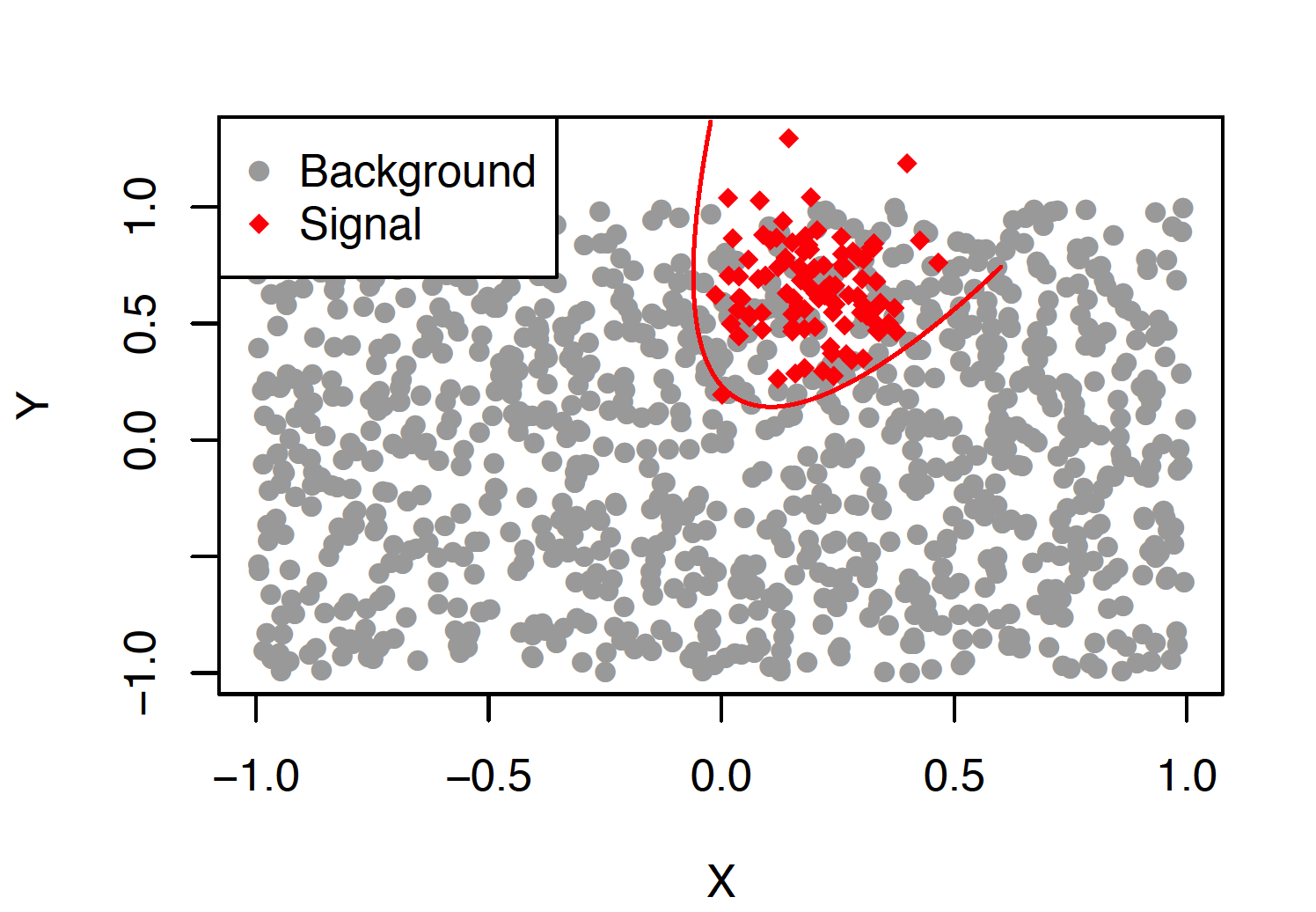
(a) Training Samples

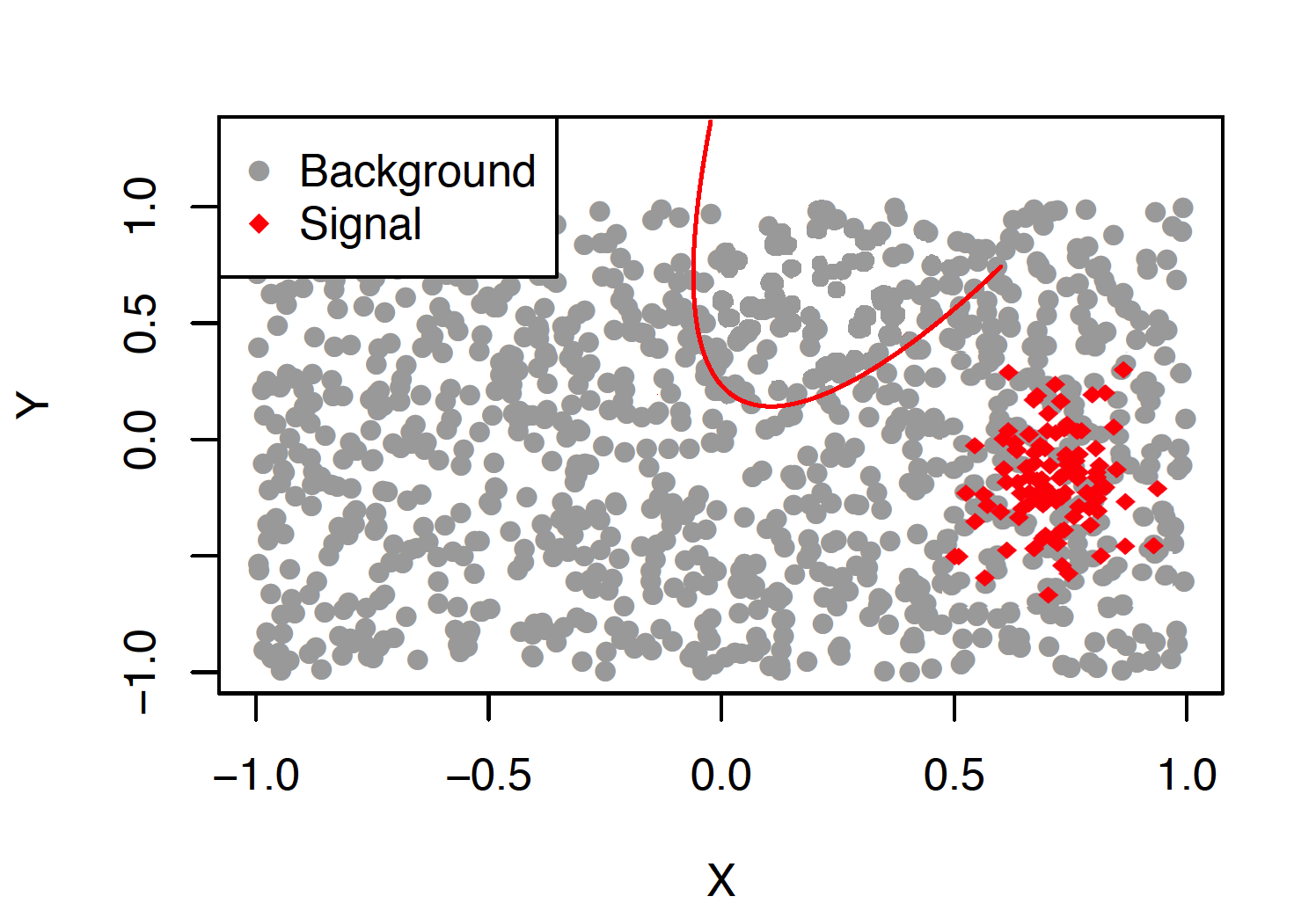
(b) Experimental Samples

Figure 1: Decision boundary using a supervised classifier to separate the signal (red rhombuses) from the background (grey). (a) The decision boundary of the classifier when trained on signal generated from the assumed signal model. (b) When the signal model is mis-specified, the classifier completely misses the actual signal data when used on the experimental samples. We consider a two-dimensional example here for illustration purposes only. The real data can be of much higher dimensionality. In the experiments considered in this paper, we have a 16-dimensional sample.

But there are disadvantages to this approach. First, this approach may have trouble finding novel, unexpected deviations from the background model. Second, a search targeting one kind of new physics signal/scenario is not going to be powerful for finding a different new physics signal/scenario. Figure 1 illustrates the problem. If a classifier is trained on training signal data as shown in Figure 1(a), it gives the classification boundary as shown. But what if the signal in the experimental data actually looks like Figure 1(b)? Then the classifier ends up misclassifying the signal as background. So an algorithm trained on a mis-specified signal model might completely miss the actual signal. The two-dimensional example considered here is for illustration purposes only. In reality, the data lie in a high-dimensional space which further aggravates the problem.

In this paper, we study model-independent tests, which do not assume a particular signal model, and compare them to more traditional model-dependent tests for search of new physics signals. We use data from an event generator for background events together with observed experimental data, which are a mixture of background and a potential signal. But we do not use data from signal simulations. In other words, we assume access to labeled background data and unlabeled experimental data, where events may either have background or signal labels. (Note that in practice, systematic uncertainty in the background makes the situation more complex than this. Please refer to Sections 2 and 7 for further discussion.) We then use a semi-supervised approach that trains a classifier to differentiate the background data from the experimental data. Crucially, we do not assume availability of labelled signal data, which differentiates this approach from model-dependent or supervised methods.

In particular, we make the following three main contributions:

1. We propose and investigate several variants of classifier-based model-dependent and model-independent tests to detect a new signal in the experimental data. These tests involve four steps:

   1. Training a probabilistic classifier to differentiate between background events and potential new signal events in the model-dependent mode and to differentiate between background events and experimental events in the model-independent mode.

   2. Constructing classifier-based test statistics using the output of the probabilistic classifier. We construct four different test statistics, using two different strategies, and compare them.

   3. Estimating the null distributions of the test statistics using asymptotic, nonparametric bootstrap, and permutation methods, and comparing them.

   4. Testing for the presence of a new signal using the test statistics and their estimated null distributions. We consider each combination of a test statistic and a method for estimating its null distribution as a separate test method.

2. We develop a method for estimating the signal strength in the experimental data, which is a challenging problem in model-independent searches since we do not have information about the signal model to characterize the signal.

3. We develop active subspace methods to interpret the signal detected by the semi-supervised classifier in the high-dimensional space.

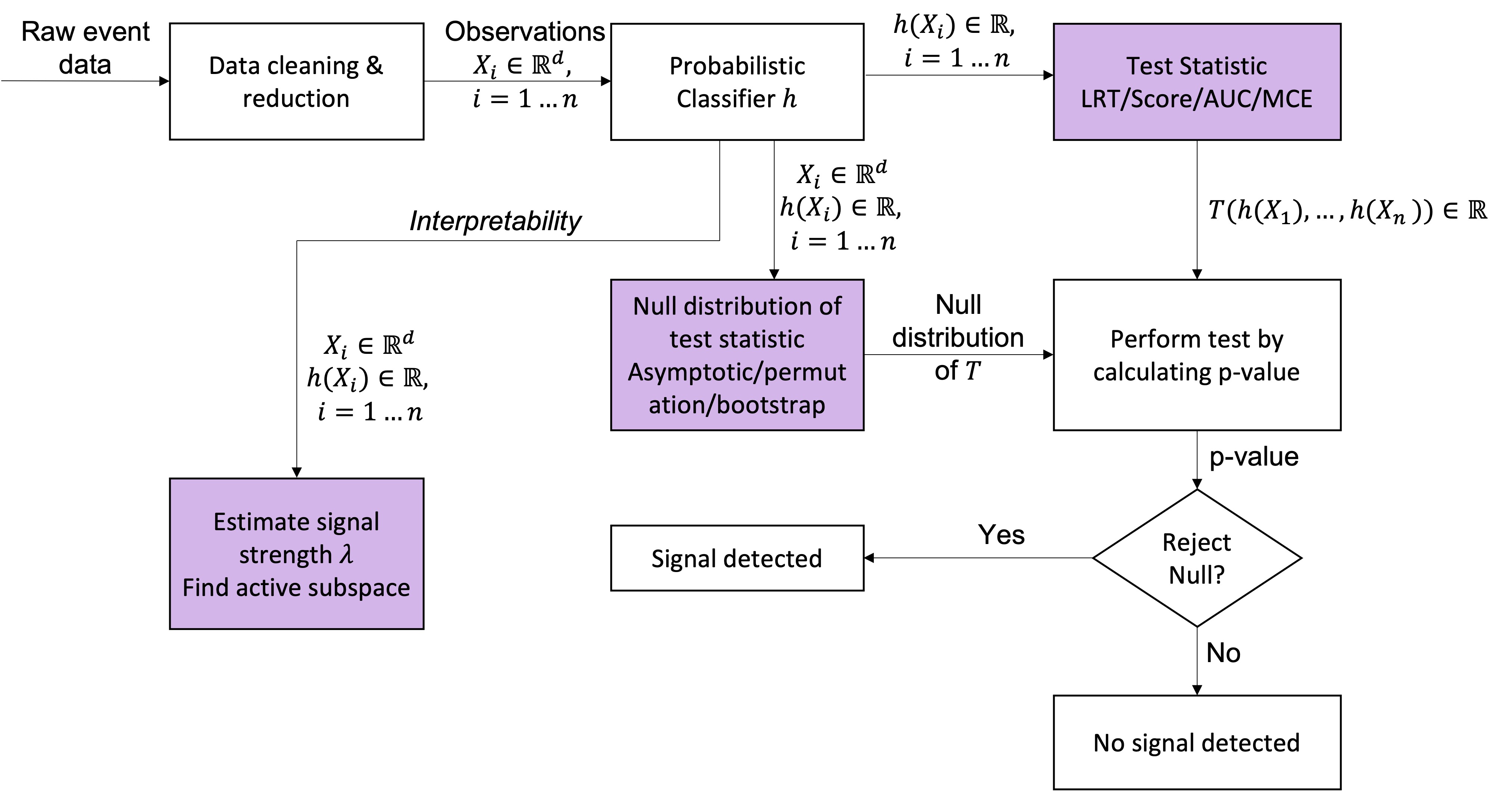
Figure 2: Data flow diagram presenting the signal detection approach, including the interpretability of the trained classifier, from raw data to concluding whether there is any signal in the data. The colored boxes represent our contributions presented in this paper. The raw data and data reduction steps are presented, e.g., in Adam-Bourdarios et al. (2015).

The data flow diagram presented in Figure 2, illustrates the signal detection approach in four stages: training the probabilistic classifier, computing the test statistics, estimating the null distribution of the test statistics and finally performing the test. There is also the stage where we use the fitted classifier to estimate the signal strength and interpret the classifier using active subspace methods. The colored boxes in the diagram represent our contributions in this paper, namely introducing the different test statistics, introducing methods to estimate the null distribution, estimating the signal strength, and interpretability via active subspace methods. The diagram also demonstrates how the dimensionality of the data reduces from observations (16-D in our case) to the classifier outputs (1-D) which are then used to find the scalar test statistics. Below we detail selected parts of our approach.

Training a probabilistic classifier. The approach we take is one introduced by particle physicists in the model-dependent mode, where we first train a probabilistic classifier ($h$) and then use its output to construct the test statistics. In the model-dependent (MD) mode, the classifier ($h$) finds differences between the properties of simulated background data and simulated signal data. The classifier ($h$) is then applied on the experimental data ($W_{i}$’s) and the output $(h(W_{i}))$ is used to construct the test statistics. In the model-independent (MI) mode, we do not make assumptions about the signal model, and hence do not have access to simulated signal data. So, the classifier instead is trained to find differences between the simulated background data and the experimental data, and if it is able to differentiate between them, it indicates the presence of a signal component in the experimental data.

Constructing classifier-based test statistics. We propose two different strategies to construct test statistics from the probabilistic classifier. Using each of the two strategies, we then construct two test statistics. The first strategy, creating density ratio based test statistics, takes advantage of the fact that for a probabilistic classifier, the output $h$ is the posterior binary class probability. Now, the posterior probability ($h(w)$) can be written as a one-to-one function of the ratio ($\psi(w)$) of the probability densities of the two classes. Hence, the density ratio $\psi(w)$ can be estimated using the classifier output $h(w)$. Using these density ratio estimates, we create two classical test statistics – the likelihood ratio test statistic (LRT) and the score statistic. Note that the two classes are background and signal in the MD mode and background and experimental in the MI mode. This strategy leverages the fact that classifiers have been found to give accurate estimates of density ratios (Cranmer, Pavez and Louppe, 2015).

The second strategy is to construct classification performance based test statistics. This strategy, which is only applicable in the MI setting, takes advantage of the fact that in the MI mode, in the absence of a signal in the experimental data, a classifier should not be able to differentiate the experimental data from the background data, since they have the same distribution. This is analogous to a high-dimensional two-sample testing problem where we compare the distributions of the background and the experimental data using a classifier (Friedman, 2003; Kim et al., 2016, 2019). In this case, the performance of the classifier is indicative of whether there is any signal in the data. We measure the performance in two ways, resulting in two test statistics – the area under the ROC curve (AUC) and the misclassification error (MCE). The reason we include these test statistics is because they are properties of the classifier itself in contrast to the LRT which is being estimated using the classifier.

The four test statistics according to the two strategies are presented in Table 1. In the model-dependent mode we cannot use classification performance based test statistics since the classifier is trained on background and signal data. In the model-independent mode, we cannot use the score statistic. This is because the score statistic is a function of the density ratio of the signal data and the background data, whereas, in the model-independent setting, we only have an estimate for the density ratio of the experimental data and the background data.

Table 1: Test statistics considered for model-dependent (MD) and model-independent (MI) searches.“X” marks cells that do not have a corresponding test statistic.

	Test Statistics
	Density Ratio Based			Classification Performance Based
	LRT	Score		AUC	MCE
Model-dependent	MD-LRT	MD-Score		X	X
Model-independent	MI-LRT	X		MI-AUC	MI-MCE

One of our model-independent tests based on the LRT statistic is similar to the test proposed by D’Agnolo and Wulzer (2019) and D’Agnolo et al. (2021). The other two model-independent test statistics are the AUC and MCE statistics. To the best of our knowledge, these two are novel in this application. Though the test that uses the LRT is similar to the test proposed by D’Agnolo and Wulzer (2019) and D’Agnolo et al. (2021), unlike them, we use the nonparametric bootstrap as well as permutation methods to estimate the null distribution, comparing the performance of the different re-sampling techniques. We also apply the tests in a higher-dimensional setting than them. Additionally, since our test has a simple null versus a composite alternative, the LRT is not guaranteed to yield an optimal test in this setting. Hence, it is important to compare the performance of the different test statistics.

Estimating the null distributions and Testing. We estimate the null distributions of the test statistics using four different approaches - asymptotic, nonparametric bootstrap, permutation, and slow permutation. The bootstrap and permutation approaches are resampling methods that utilize the fact that under the null, the experimental data and the background data have the same distribution and so, the data can be resampled from a combination of the two data sets and their labels can be permuted. The bootstrap and the regular permutation method split the data into training and test data sets and re-sample the test data sets only, whereas the slow permutation method re-samples the entire data set and re-trains the classifier on each re-sampled data set, which increases its computational complexity. A combination of a test statistic and a null distribution estimation method forms a test. In principle, every test statistic has a true null distribution, which these methods are trying to estimate. So, under the null, these methods should give similar distributions. However, it is important to note that the estimated null distribution is a function of the experimental data, and hence only when there is no signal in the experimental data (when null is true), it estimates the true null distribution. So, the power of the tests, when there is signal, is expected to be different for the different null estimation methods. Hence, it is important to compare the performance of the different null estimation methods for the different test statistics.

Estimating the signal strength. Towards our second contribution of estimating the signal strength, the problem is particularly challenging in the MI mode, since the classifier differentiates between background and experimental data, and hence cannot directly identify signal events. We solve this by showing that estimating the signal strength is equivalent to estimating a monotone univariate density over the interval $[0,1]$ at the right boundary at 1. In particular, we need to estimate the density of a statistic built by considering the quantile of a Neyman–Pearson-style likelihood ratio. Similar to the estimator given by Storey (2002), which is a special case of a boundary density estimator using histograms, we use histograms to estimate the density, and then use a Poisson regression (Nelder and Wedderburn, 1972) model of the histogram bin counts to estimate the density at the boundary point. The additional use of Poisson regression makes the boundary estimate more stable. We also find confidence intervals for the estimates using GLM regression intervals and three different bootstrap methods.

Active subspace methods. For our third contribution, to interpret the classifier and characterize the signal, we propose using active subspace methods (Constantine, Dow and Wang, 2014; Constantine, 2015) to explore which aspects of the covariates are the most informative for the test. Active subspaces have been used as a form of sensitivity analysis to quantify uncertainty in an output (Constantine et al., 2015) and they have also been used to analyze the internal structure and vulnerability of deep neural networks (Cui et al., 2020). Similar to these works, in this paper, we propose active subspace methods to interpret the variability in the classifier output in terms of its inputs. Our proposed methods identify the directions that capture the most variability in the gradient of the classifier. These directions are found using an eigen decomposition (PCA) of the gradients of the classifier surface at observed points. These directions give us information about the combinations of the covariates that most influence the classifier in distinguishing the experimental data from the background data, hence giving us an idea of what the signal looks like. Importantly, this process helps us better understand the classifier that detects the signal, which otherwise would be a black box.

Alternative variable importance methods have been used to understand the intrinsic predictiveness potential of the covariates (Van der Laan, 2006; Lei et al., 2018; Williamson et al., 2020) which identify the individual covariates that play an important role in the classifier. Variable importance has been addressed extensively for random forests (Breiman, 2001; Ishwaran et al., 2007; Strobl et al., 2008; Grömping, 2009) and neural networks (Bach et al., 2015; Shrikumar, Greenside and Kundaje, 2017; Sundararajan, Taly and Yan, 2017). But contrary to the active subspace methods, these methods concentrate on finding the variables that are individually the most important and potentially miss detecting combinations of covariates that might have more predictive power.

It is worth noting that the methods presented in this paper can also be applied more generally. In this paper, we demonstrate an application of the methods to the search of new phenomena in particle physics, but the methods presented here are applicable beyond particle physics. In general, these methods can be applied whenever there is a need to search for, detect or characterize collective anomalies in a high-dimensional space, where a single data point is not necessarily anomalous but a collection of data points is. For example, these methods could potentially be used to find anomalous weather changes in high-dimensional climate science data sets, where individual weather events might themselves not be anomalous but a collection of certain types of weather events over a period of time might be. Potential further applications range from engineering to medicine and other areas of the physical sciences.

The rest of this paper is structured as follows. In the following section, we describe the role of model-independent methods in the search for new physics phenomena and discuss some existing literature on it. In Section 3, we introduce the problem setup mathematically. We describe the MD methods in Section 3.1 and the proposed MI methods in Section 3.2. We then discuss methods to estimate the signal strength in the experimental data in Section 4. In Section 5, we describe active subspace methods to understand the subspace affecting the classifier the most, leading to an understanding of the detected signal. Finally, in Section 6, we demonstrate the performance of the proposed MI methods and compare them to the MD methods using publicly available simulated data from a machine learning data challenge that includes events corresponding to the SM Higgs boson signal. We include concluding remarks and possible future directions of research in Section 7. We also provide exploratory analysis of the Higgs boson data set that is used to perform the experiments in Section 6 and include some other experimental details in the Supplementary Material (Chakravarti et al., 2022). We defer the proofs of the theorems and some of the proposed algorithms to the Supplementary Material as well.

2 Overview of Model-Independent Searches of New Physics

In particle physics, before any search analysis is performed, the experimental data is typically filtered for specific types of final-state particles. Different choices here specify different search channels. For example, the search could be restricted to a decay channel where four muons are observed. The data set would then contain kinematic and other features of these particles observed using the particle detector, which dictates the dimensionality of the data. The data set is further restricted by selection cuts on these features that are used to remove data points that lie in regions of the phase space that are believed to be signal-free. For example, one might choose only those events where the particles have large transverse momenta (larger than some threshold). These cuts are generally performed to increase the signal-to-background ratio in the final experimental data that is considered in the analysis. Even after the selection cuts, a typical data set that needs to be analyzed may have a sample size ranging from hundreds of thousands of events to million or billions of events. All of the methods presented in this paper can handle such large data sets (as demonstrated in Section 6). In the experiments performed in this paper, we use a 16-dimensional data set which is also typical for the searches, although the dimensionality can also be much larger for complex search channels or if low-level detector information is used.

Most model-independent approaches find the signal in experimental data by comparing it to a reference background dataset, which is an essential requirement for these strategies. Hence, it is necessary for these approaches to have a trustable reference dataset. As discussed in D’Agnolo et al. (2022), it is conceptually unavoidable for these model-independent approaches to require a reference background dataset, since they search for “new” phenomena, and hence require a necessary notion of “old” phenomena. The required reference background datasets are usually generated using Monte Carlo event generators, which sample collision events consistent with the equations of the Standard Model of particle physics. Some recent approaches, such as ANODE (Nachman and Shih, 2020) and CWoLa (Classification Without Labels) Bump Hunting (Collins, Howe and Nachman, 2018, 2019), estimate the background from the data itself, which requires assumptions on the signal region and access to data not in the signal region. Here we do not make any assumptions on the signal region, so we use Monte Carlo simulations from the Standard Model as the reference background dataset. However, it is good to note that model-independent approaches are not necessarily restricted to Monte Carlo backgrounds, as demonstrated by ANODE and CWoLa.

Even though these model-independent approaches are dependent on the availability of a reliable, trustable background dataset to find new phenomena, the key advantage of model-independent approaches is that they can detect discrepancies between the background data and the experimental data irrespective of the distribution of the signal events. Such capability can be essential for ensuring the maximal reach of the LHC physics program. In the case that a discrepancy is found, it should be investigated further in order to understand if it results from (a) an inaccurate background MC generator, (b) a particle detector defect or a lack of understanding of the detector, or (c) a previously unknown physics process. The active subspace methods proposed in this paper may provide a preliminary indication in this process. A model-independent search indicating a significant discrepancy can also guide the selection of new model-dependent analyses to further investigate the nature of the discrepancy.

It is important to note here that there is no one “right” approach to finding new physics signals. The different model-dependent and model-independent approaches are complementary and not superior to each other. For example, when a reliable signal model is available, model-dependent approaches should yield greater power since they use the information available about the signal model to optimize the test. It is also good to note that there is no black-and-white distinction between model-independent and model-dependent methods. Rather, there is a continuum of methods that vary in terms of the strength of the assumptions involved. Any “model-independent” method at minimum needs to make assumptions about the background. Furthermore, to perform the model-independent search, one would in practice use some amount of physics knowledge to choose a particular decay channel (say, 4 muons) and to impose further cuts within that channel (e.g., to choose events where the particles have large transverse momenta) to narrow down the search to a part of the phase space that is believed to be fertile for new signals and where the background can be modeled sufficiently well. One might then be willing to make further assumptions about the location or shape of the signal region, and so on. At the far end of this spectrum are fully “model-dependent” methods that assume a specific signal model.

Additionally, both model-independent and model-dependent methods are affected by systematic uncertainties in the background (Cranmer, 2015; Lyons and Wardle, 2018; Dorigo and de Castro, 2020). Background systematics in high-energy physics are typically parameterized using nuisance parameters that affect, among other things, the rate and shape of the background samples. In low-dimensional situations, a standard approach is to handle these nuisance parameters using likelihood profiling (Cranmer, 2015), while recent work has focused on incorporating nuisance parameters into classifier training for high-dimensional data. Training a classifier on simulated data generated using specific values for the nuisance parameters may not be optimal for handling background data generated using other values of the nuisance parameters. Even if the classifiers are trained on data generated using the most likely values of the nuisance parameters, and their effect is accounted for in the calibration, the power of the methods to detect new signals may be affected (Dorigo and de Castro, 2020). Some classifier-based model-dependent approaches have been recently suggested to handle the nuisance parameters. For example, Ghosh, Nachman and Whiteson (2021) profile the nuisance parameters by constructing classifiers that are explicitly dependent on the different values of the nuisance parameters. Reviews of model-dependent approaches that deal with nuisance parameters in classifier-based searches can be found in Nachman (2020) and Dorigo and de Castro (2020). Overall, dealing with systematic uncertainties in the background in the model-independent setting is a challenging problem that affects any model-independent method and whose detailed treatment is beyond the scope of this paper. However, we note there is no reason to believe that it would not be possible to extend existing approaches for handling background systematics from the model-dependent setting into the model-independent case. D’Agnolo et al. (2022) is, to the best of our knowledge, a first contribution toward this important goal.

Below, we present a non-exhaustive review of existing literature on model-independent approaches and other related work.

2.1 Related Literature

Due to their advantages, model-independent approaches have been used for new physics searches (Knuteson, 2000; CDF Collaboration, 2008; Soha, 2008) at the Tevatron (Choudalakis, 2008; CDF Collaboration, 2009; D0 Collaboration, 2012c), HERA (H1 Collaboration, 2004), and the LHC (CMS Collaboration, 2017; ATLAS Collaboration, 2019; CMS Collaboration, 2020). These methods typically compare a large set of binned distributions to the prediction from the background Monte Carlo simulation, in search for bins in the experimental data that exhibit a deviation larger than some predefined threshold. For example, the approach of ATLAS Collaboration (2019), employed by the ATLAS experiment, uses a (quasi-)model-independent method that considers some generic features of the potential new physics signals. These approaches have two limitations: (a) they do not consider the multivariate dependency structures between the variables in the data and (b) they might miss certain signals that do not show a localized excess in one of the studied distributions.

More recent approaches like CWoLa (Classification Without Labels) Bump Hunting (Collins, Howe and Nachman, 2018, 2019), ANODE (Nachman and Shih, 2020), SALAD (Andreassen, Nachman and Shih, 2020) and simulation augmented CWoLa (SA-CWoLa) (Kasieczka et al., 2021) are also based on searching for anomalies by assuming that the signal is localized in a single feature. These approaches use this weak assumption about the signal which causes them to have the second limitation mentioned above, namely they might miss signals that do not show a localized excess along one of the features. Some of the algorithms additionally assume that the signal’s distribution for the other features is independent of the selected single feature that is being scanned. Kasieczka et al. (2021) describes a variety of current methods for signal detection along with results on the LHC Olympics 2020 datasets.

A different approach that uses a semi-supervised nonparametric clustering algorithm is presented by Casa and Menardi (2018). They assume that in high energy physics, a new particle manifests itself as a significant peak emerging from the background process. They use nonparametric modal clustering to search for a signal that is expected to emerge as a bump in the background distribution. BuHuLaSpa and Bump Hunter methods presented in Kasieczka et al. (2021) also use similar bump hunting ideas to find the signal. UCluster presented in Kasieczka et al. (2021) uses clustering to find the localized signal. These methods suffer from the second problem mentioned above: they can only find localized signals.

Model-independent semi-supervised searches were also proposed by Kuusela et al. (2012) and Vatanen et al. (2012) who use multivariate Gaussian mixture models to estimate the densities of the background and the experimental data. They test for the significance of the additional Gaussian components which quantify the anomalous contribution. The drawback of this method is that Gaussian mixture models are very difficult to fit in a high-dimensional setting. Additionally, since the signal strength is typically very small, the quality of the fit influences the power of the test in detecting the signal.

These drawbacks of the mixture modeling methods along with the fact (as mentioned before) that classification algorithms have demonstrated excellent performance in detecting signals in the model-dependent approaches, especially in the high-dimensional setting, motivates us to use classifiers instead of mixture modeling to find the deviations of the experimental data from the background.

The problem of comparing the distributions of the background and the experimental data is also analogous to a high-dimensional two-sample testing problem (Kim et al., 2016, 2019), where the signal events appear as a collective anomaly (Chandola, Banerjee and Kumar, 2009) in a cluster close to each other. Hence, we also compare the methods proposed in this paper to nearest-neighbor two-sample tests introduced in Schilling (1986) and Henze (1988) for a sub-sample of the data. In the experiments, we observe that methods that use a semi-supervised classifier have much higher power to detect the signal than the nearest-neighbor two-sample tests.

3 Classifier-Based Tests for Signal Detection

In this section, we introduce both model-dependent and model-independent approaches to signal detection in the experimental particle physics data. Both approaches use background data from MC event generators for background events based on the Standard Model, together with experimental data, which are a mixture of background and a potential signal. First, we discuss the model-dependent approach that additionally assumes access to signal data that are generated using MC event generators for a hypothesized signal model. Then we describe the model-independent approach that does not assume access to the signal data. We now introduce formal notation to discuss the two different approaches.

The background, signal and experimental data are samples from Poisson point processes (Cranmer, 2015; Reiss, 2012). We condition on the sample sizes of the individual datasets so that the data in all three of the cases may be treated as independent samples from a density (i.e., from a binomial point process). Specifically, we have three datasets:

Background: $$\quad\mathcal{X}=\{X_{1},\ldots,X_{m_{b}}\}, \quad X_{i}\sim p_{b}$$

Signal: $$\quad\mathcal{Y}=\{Y_{1},\ldots,Y_{m_{s}}\}, \quad Y_{i}\sim p_{s}$$ (1)

Experimental: $$\quad\mathcal{W}=\{W_{1},\ldots,W_{n}\}, \quad W_{i}\sim q=(1-\lambda)p_{b}+\lambda p_{s},$$

where $p_{b},p_{s}$ are the densities of the background and signal data respectively, $q$ is the density of the experimental data and $\lambda$ is a scalar parameter representing the signal strength.

The likelihood function for $\lambda$ given the experimental data ($\mathcal{W}$) (treating $p_{b}$ and $p_{s}$ as known for the moment) is

$${\cal L}(\lambda)=\prod_{i}((1-\lambda)p_{b}(W_{i})+\lambda p_{s}(W_{i})).$$ (2)

The null hypothesis ($H_{0}$) that there is no signal corresponds to $\lambda=0$. So the goal is to test $H_{0}:\lambda=0$ versus $H_{1}:\lambda>0$. We additionally have the likelihood ratio:

$$\frac{{\cal L}(\lambda)}{{\cal L}(0)}=\prod_{i}(1-\lambda+\lambda\psi(W_{i}))$$ (3)

where $\psi(w)=p_{s}(w)/p_{b}(w)$. Note that the function $\psi$ can be seen as an infinite dimensional nuisance parameter.

In the idealized case where $p_{b}$ and $p_{s}$ are known, we could use the usual likelihood ratio test (LRT) statistic

$$T=-2\log({\cal L}(0)/{\cal L}(\widehat{\lambda}))=2\sum_{i}\log(1-\widehat{\lambda}+\widehat{\lambda}\psi(W_{i})),$$ (4)

where $\widehat{\lambda}$ is the maximum likelihood estimator (MLE) of $\lambda$ based on the experimental data $\mathcal{W}$. Alternatively, we could use the score test statistic

$$\mathcal{T}=\frac{1}{n}\sum_{i}(\psi(W_{i})-1).$$ (5)

In practice, the densities $p_{b}$ and $p_{s}$ are unknown. The two different approaches described in this section show how a classifier can be used to estimate the desired statistics directly. We prefer estimating the density ratio required for the desired statistics directly instead of taking the ratio of the estimated densities. This is due to the high-dimensionality of the data which makes estimating the high-dimensional density with limited data very difficult.

3.1 The Model-Dependent (Supervised) Case

In this case, we make use of the signal data $\mathcal{Y}$, where $Y_{1},\ldots,Y_{m_{s}}\sim p_{s}$ are generated using a MC event generator for a hypothized signal model. Such approach is standard in most new physics searches at the LHC, and serves here as a point of comparison against the model-independent methods. The strategy underlying our implementation of this approach is to use a classifier to estimate $\psi=p_{s}/p_{b}$ and then use the LRT or the score test with the estimated $\psi$. Since $\psi$ is estimated, we cannot rely on standard asymptotics to get the null distribution. Instead we use permutation or nonparametric bootstrap methods.

Before we train a classifier, we first combine the background and signal data into a single dataset

$$\{Z_{1},\ldots,Z_{m_{b}+m_{s}}\}=\mathcal{X}\cup\mathcal{Y}=\{X_{1},\ldots,X_{m_{b}},Y_{1},\ldots,Y_{m_{s}}\}$$

and we define $S_{i}=1$ if $Z_{i}$ is from the signal data $\mathcal{Y}$ and $S_{i}=0$ otherwise. We treat $(Z_{i},S_{i})$ as a sample from a density $p(z,s)$ with $\pi_{0}:=\mbox{$\mathbb{P}$}(S=1)=m_{s}/(m_{b}+m_{s})$, the probability of any sample being from the signal distribution.

Let $h_{0}(z):={\mbox{$\mathbb{P}$}}\left(S=1|Z=z\right)$ denote the probability of a sample being from the signal distribution given $Z=z$. Then using Bayes’s rule,

$$h_{0}(z)={\mbox{$\mathbb{P}$}}\left(S=1|Z=z\right)=\frac{\pi_{0}\psi(z)}{\pi_{0}\psi(z)+(1-\pi_{0})}.$$ (6)

Inverting this,

$$\psi(z)=\left(\frac{1-\pi_{0}}{\pi_{0}}\right)\left(\frac{h_{0}(z)}{1-h_{0}(z)}\right).$$ (7)

This leads to our estimate of $\psi$,

$$\widehat{\psi}(z)=\left(\frac{1-\pi_{0}}{\pi_{0}}\right)\left(\frac{\widehat{h}_{0}(z)}{1-\widehat{h}_{0}(z)}\right),$$ (8)

where $\widehat{h}_{0}(z)$ is a classifier that separates the signal data $\mathcal{Y}$ from the background data $\mathcal{X}$. In this paper, we take $\widehat{h}_{0}$ to be a random forest, but in principle, any classifier can be used.

To use $\widehat{\psi}(z)$ to calculate the LRT statistic in (4), we estimate $\lambda$ using its MLE as follows. We can write the likelihood of the experimental data as

$${\cal L}(\lambda)=\prod_{i}p_{b}(W_{i})\times\prod_{i}(1-\lambda+\lambda\psi(W_{i})).$$ (9)

The first term does not involve $\lambda$ so we can ignore it. Hence,

$${\cal L}(\lambda)\propto\prod_{i}(1-\lambda+\lambda\psi(W_{i})).$$ (10)

We then define the estimated likelihood

$$\widehat{\cal L}(\lambda)\propto\prod_{i}(1-\lambda+\lambda\widehat{\psi}(W_{i}))$$ (11)

and we define $\widehat{\lambda}$ to be the maximizer of $\widehat{\cal L}(\lambda)$. We can now use $\widehat{\lambda}$ and $\widehat{\psi}$ to estimate the LRT and the score test statistics as given in (4) and (5).

To see the effect of maximizing the estimated likelihood using the estimated $\psi$ instead of maximizing the actual likelihood, let $\ell(\lambda)=\log{\cal L}(\lambda)$, let $\widehat{\ell}(\lambda)=\log\widehat{\cal L}(\lambda)$, and note that, for small $\lambda$

$$\ell(\lambda)=\lambda\sum_{i}(\psi(W_{i})-1)-\frac{\lambda^{2}}{2}\sum_{i}(\psi(W_{i})-1)^{2}+o_{P}(\lambda^{2})+C,$$ (12)

where $C=\sum_{i}\log(p_{b}(W_{i}))$ is just a constant and can be ignored. A similar relation holds for $\widehat{\ell}(\lambda)$ and $\widehat{\psi}$. So

$$\frac{1}{n}\widehat{\ell}(\lambda)-\frac{1}{n}\ell(\lambda)=\frac{\lambda}{n}\sum_{i}(\widehat{\psi}(W_{i})-\psi(W_{i}))+o_{P}(\lambda)$$ (13)

which shows how the accuracy of the classifier affects the log-likelihood. The maximizer $\widetilde{\lambda}$ of $\ell(\lambda)$ and the maximizer $\widehat{\lambda}$ of $\widehat{\ell}(\lambda)$ are

$$\widetilde{\lambda}=\left[\frac{\sum_{i}(\psi(W_{i})-1)}{\sum_{i}(\psi(W_{i})-1)^{2}}\right]_{+}+o_{P}(\lambda),\ \ \ \ \ \widehat{\lambda}=\left[\frac{\sum_{i}(\widehat{\psi}(W_{i})-1)}{\sum_{i}(\widehat{\psi}(W_{i})-1)^{2}}\right]_{+}+o_{P}(\lambda).$$ (14)

Hence, $\widehat{\lambda}-\widetilde{\lambda}=O_{P}(\frac{1}{n}\sum_{i}(\widehat{\psi}(W_{i})-\psi(W_{i})))$, emphasizing again the importance of an accurate classifier. Note that in practice, instead of using the above approximation, we evaluate the MLE of $\lambda$ by performing a grid search on $[0,1]$.

As $n\to\infty$, the usual likelihood ratio test statistic (Ghosh and Sen, 1984; Böhning et al., 1994),

$$T=2\sum_{i}\log\left((1-\widehat{\lambda})+\widehat{\lambda}\psi(W_{i})\right)\overset{d}{\rightsquigarrow}\frac{1}{2}\delta_{0}+\frac{1}{2}\chi^{2}_{1},$$ (15)

where $\delta_{0}$ is a degenerate distribution at $0$. But when $\widehat{\psi}$ is substituted for $\psi$, the asymptotic distribution is unknown so the null distribution needs to be estimated by simulating from the background model. If the available background data is limited, we can use permutation or nonparametric bootstrap methods; see Section 6.2.

Similar remarks apply to the score statistic $\mathcal{T}=n^{-1}\sum_{i}(\psi(W_{i})-1)$ and its estimated version $\widehat{\mathcal{T}}=n^{-1}\sum_{i}(\widehat{\psi}(W_{i})-1)$. There are conditions under which $\widehat{\mathcal{T}}$ has a tractable distribution. Suppose that $\widehat{\psi}$ is estimated on part of the data and $\widehat{\mathcal{T}}$ on another. Now

$$\sqrt{n}\widehat{\mathcal{T}}=\sqrt{n}\mathcal{T}+\sqrt{n}\left(\frac{1}{n}\sum_{i}\left(\widehat{\psi}(W_{i})-\psi(W_{i})\right)\right).$$ (16)

The first term converges to $N(0,\sigma^{2})$ where $\sigma^{2}=\mathbb{E}_{p_{b}}[(\psi(W)-1)^{2}]$. If $\psi$ is in a Hölder class of smoothness index $\beta$ and $\beta>d/2$, then it can be shown that $\frac{1}{n}\sum_{i}(\widehat{\psi}(W_{i})-\psi(W_{i}))=O_{P}(n^{-2\beta/(2\beta+d)})$, where $d$ is the dimension of the $W_{i}$’s. Hence, if $\beta>d/2$, the second term is negligible so that $\sqrt{n}\widehat{\mathcal{T}}\rightsquigarrow N(0,\sigma^{2})$. However, we have found that the Normal approximation is poor in practice and instead we use permutation and bootstrap methods to approximate the null distribution. Similar to the LRT, the null distribution can also be estimated by simulating from the background model.

To use nonparametric bootstrap or permutation methods, we randomly split the available background data $\mathcal{X}$ into two sets $\mathcal{X}_{1}$ and $\mathcal{X}_{2}$. We use the first set $\mathcal{X}_{1}$ along with the signal data $\mathcal{Y}$ to train the classifier $\widehat{h_{0}}$. We use the second set $\mathcal{X}_{2}$ along with the experimental data $\mathcal{W}$ to approximate the null distributions of the LRT and the score statistics. Note that, under the null $H_{0}:\lambda=0$, the experimental data $\mathcal{W}$ and background data $\mathcal{X}_{2}$ have the same distribution $p_{b}$. In the case of nonparametric bootstrap, we approximate the null distributions by repeatedly sampling with replacement from $\mathcal{X}_{2}\cup\mathcal{W}$, and computing the test statistics. For the permutation test, we do the same using sampling without replacement.

3.2 Model-Independent (Semi-Supervised) Case

In this case, we assume that we do not have access to (or do not completely trust) the signal training sample $\mathcal{Y}=\{Y_{1},\ldots,Y_{m_{s}}\}$. So the data available are $\mathcal{X}=\{X_{1},\ldots,X_{m_{b}}\}$ and $\mathcal{W}=\{W_{1},\ldots,W_{n}\},$ where $X_{i}\sim p_{b}$ and $W_{i}\sim q=(1-\lambda)p_{b}+\lambda p_{s}$, with $p_{b}$, $p_{s}$ and $\lambda$ unknown. We want to test $H_{0}:\lambda=0$ versus $H_{1}:\lambda>0$ which is equivalent to testing $H_{0}:p_{b}=q$ versus $H_{1}:p_{b}\neq q$. Hence we are in a two-sample testing scenario (Kim et al., 2016, 2019).

Again, we want to leverage the fact that classifiers have been found to give accurate estimates of density ratios (Hastie, Tibshirani and Friedman, 2009, Ch.14) (Goodfellow et al., 2014; Cranmer, Pavez and Louppe, 2015). One strategy is to use a classifier like before to obtain a likelihood ratio test statistic, but this time we estimate the density ratio $\psi^{\dagger}=q/p_{b}$. To do this, we train a classifier to differentiate between the experimental ($\mathcal{W}$) and background events ($\mathcal{X}$) instead of the signal ($\mathcal{Y}$) and background events ($\mathcal{X}$) . As mentioned in the introduction, this strategy is similar to the one taken by D’Agnolo et al. (2021) and D’Agnolo and Wulzer (2019), who use a neural network to estimate the likelihood ratio test statistic.

A second strategy is to use the area under the curve statistic (AUC) (Hanley and McNeil, 1982) or the misclassification error/misclassification rate (MCE) to evaluate the performance of the classifier. The intuition behind the second strategy is that in the absence of signal under the null, a classifier should not be able to differentiate between the background and the experimental data. We discuss both the strategies below.

As before, let $h$ denote a classifier in the combined (background and experimental) sample, then

$$\psi^{\dagger}(z)=\left(\frac{1-\pi}{\pi}\right)\left(\frac{h(z)}{1-h(z)}\right)$$ (17)

where now $\pi=n/(n+m_{b})$. This leads to our estimate of $\psi^{\dagger}$

$$\widehat{\psi^{\dagger}}(z)=\left(\frac{1-\pi}{\pi}\right)\left(\frac{\widehat{h}(z)}{1-\widehat{h}(z)}\right)$$ (18)

where $\widehat{h}(z)$ is the trained classifier.

The likelihood ratio as given in (3) can be rewritten as

$$\frac{\mathcal{L}(\lambda)}{\mathcal{L}(0)}=\prod_{i}\psi^{\dagger}(W_{i}).$$ (19)

Hence, the LRT statistic is given by

$$T=2\sum_{i}\log\widehat{\psi^{\dagger}}(W_{i}).$$ (20)

Similar to the arguments presented in the model-dependent case, since we are estimating $\psi^{\dagger}$ using $\widehat{\psi^{\dagger}}$, usual asymptotics do not hold for the LRT statistic. Instead we propose a conditional asymptotic test. We split the background and the experimental data into training and test data and estimate $\widehat{h}$ on the training data. We then use the test experimental data to calculate the test statistic $T$ and use the test background data to approximate the null distribution. Unlike the chi-squared null distribution considered by D’Agnolo et al. (2021) and D’Agnolo and Wulzer (2019), we instead use an asymptotic Normal distribution to approximate the null distribution. In this paper, the split of the data into training and test data sets is performed roughly equally. The reason for this is that if the size of the training data is small, we might not have sufficient signal samples in the training data for the classifier to recognize them, and if the size of the test data is small, there might not be enough signal samples in the test set for the test to give a significant result. We additionally propose nonparametric bootstrap and permutation methods to approximate the null distribution as well.

For the second strategy that uses the performance of the classifier ($\widehat{h}$) in separating the background data from the experimental data, we consider two statistics - AUC (Area Under the Curve) statistic and MCE (Misclassification Error) statistic.

A conventional summary of the ROC curve is the Area Under the Curve, or AUC. The ROC curve (Metz, 1978; Hanley et al., 1989) demonstrates the performance of a classifier by plotting the true positive rate (TPR) versus the false positive rate (FPR) at various threshold settings of the classifier output. For example, for our classifier $\widehat{h}(z)$, given a threshold parameter $t$, an instance $Z$ is classified as experimental (“positive”) if $\widehat{h}(Z)>t$ and background (“negative”) otherwise. Now $Z\sim q$ if $Z$ actually belongs to the experimental class and $Z\sim p_{b}$ if $Z$ actually belongs to the background class. Therefore, the TPR is given by $\mbox{TPR}(t)=\mbox{$\mathbb{P}$}_{q}\left(\widehat{h}(Z)>t\right)$ and the FPR is given by $\mbox{FPR}(t)=\mbox{$\mathbb{P}$}_{p_{b}}\left(\widehat{h}(Z)>t\right)$, where $\mbox{$\mathbb{P}$}_{q}$ is the probability when $Z\sim q$ and $\mbox{$\mathbb{P}$}_{p_{b}}$ is the probability when $Z\sim p_{b}$. Since, the ROC curve plots $\mbox{TPR}(t)$ (y-axis) versus $\mbox{FPR}(t)$ (x-axis) with varying $t$, the AUC $\theta$ is given by:

$$\theta=\int_{0}^{1}\mbox{TPR}(\mbox{FPR}^{-1}(x))\ dx=\mbox{$\mathbb{P}$}\left(\widehat{h}(W)>\widehat{h}(X)\right),$$ (21)

by standard derivation. So, the AUC can also be interpreted as the probability that a classifier will rank a randomly chosen positive instance higher than a randomly chosen negative one. Hence we can estimate it using

$$\widehat{\theta}=\frac{1}{m_{b}\ n}\ \sum_{i}\sum_{j}\ \mathbb{I}\left\{\widehat{h}(W_{j})>\widehat{h}(X_{i})\right\}.$$ (22)

Under the null $H_{0}:\lambda=0$, we have that $q=p_{b}$, i.e., $X$ and $W$ have the same distribution. So under $H_{0}$, $\theta=0.5$ and an AUC that is significantly greater than $0.5$ provides evidence of $q\neq p_{b}$. In other words, testing $H_{0}:\lambda=0$ versus $H_{1}:\lambda>0$ is equivalent to testing $H_{0}:\theta=0.5$ versus $H_{1}:\theta>0.5$.

We can also use the MCE (misclassification error/classification error rate) to measure the performance of the classifier (Kim et al., 2016), where we define the MCE as:

$$M=0.5\ \mbox{$\mathbb{P}$}(\widehat{h}(X)>\pi)+0.5\ \mbox{$\mathbb{P}$}(\widehat{h}(W)<\pi).$$ (23)

Note that this is the average of the false positive rate (first term) and the false negative rate (second term) for threshold $\pi=n/(n+m_{b})$. This can be estimated using

$$\widehat{M}=\frac{1}{2}\left[\frac{1}{m_{b}}\ \sum_{i}\ \mathbb{I}\left\{\widehat{h}(X_{i})>\pi\right\}+\frac{1}{n}\ \sum_{j}\ \mathbb{I}\left\{\widehat{h}(W_{j})<\pi\right\}\right].$$ (24)

Under the null, $H_{0}:\lambda=0$ and as a result, $q=p_{b}$, i.e., $X_{i}\overset{d}{=}W_{j}$. Hence, $M=0.5$ under the null. The classifier will have a true accuracy significantly above half (and hence $M$ below half), only if $q\neq p$. Hence we can use $\widehat{M}$ as a test statistic and test $H_{0}:M=0.5$ versus $H_{1}:M<0.5$.

As with the LRT statistic, the tests using the AUC and the MCE statistics can also be performed using asymptotic, bootstrap and permutation methods. The asymptotic AUC method, unlike the asymptotic LRT and MCE methods, does not use a conditional test. For the AUC we derive the asymptotic distribution of the statistic using results presented in Newcombe (2006). These methods also use data splitting, where we use the training data to fit the classifier ($\widehat{h}$) and use the test data to perform the test. We detail the nonparametric bootstrap and one of the permutation methods in Method 3.1 below. We provide algorithms for the other methods, including the asymptotic methods using the three statistics LRT, AUC and MCE, and the slower in-sample permutation method in the Supplementary Material (Chakravarti et al., 2022).

Remark.

1. All the model-independent methods presented in this section, except the in-sample permutation method, use data splitting of the background and the experimental data into training and test data, to approximate the null distribution and to perform the test. This has the benefit that the classifier can be kept fixed when estimating the null distribution. Here splitting a sample means randomly splitting the sample into two disjoint subsamples. The training data is used to train the classifier $\widehat{h}$ and the test data is used to perform the signal detection test. The in-sample permutation method, on the other hand, re-trains the classifier on permuted background and experimental data when approximating the null. This has the advantage of using all the data to train the classifier, but the computing time is much longer due to the classifier re-training required when obtaining the null distribution.

2. It is also important to note that here we used the random forest (RF) classifier to predict posterior probabilities. However, the “vote tallies” produced by RF classifiers are not posterior probabilities from a generative model, and very often are uncalibrated when interpreted as such. To calibrate the random forest classifier outputs, one can use methods to improve the calibration by using Platt scaling or other more sophisticated methods (Niculescu-Mizil and Caruana, 2005; Boström, 2008) on the random forest outputs before performing the tests. We performed several experiments for the model-independent asymptotic tests using Platt scaling on the random forest outputs for calibration and the results were similar to the uncalibrated random forests used here. So we leave the decision of whether to further calibrate the random forest outputs before using the tests to the discretion of the user.

Method 3.1.

Bootstrap and Permutation Methods — faster than the in-sample permutation method, but slower than the asymptotic methods. 1. Split background data ${\cal X}=\{X_{1},\ldots,X_{m_{b}}\}$ into ${\cal X}_{1}$ and ${\cal X}_{2}$ of sizes $m_{1}$ and $m_{2}$ respectively. 2. Split experimental data ${\cal W}=\{W_{1},\ldots,W_{n}\}$ into ${\cal W}_{1}$ and ${\cal W}_{2}$ of sizes $n_{1}$ and $n_{2}$ respectively, with $n_{2}=m_{2}$ 3. Train the classifier $\widehat{h}$ on ${\cal X}_{1}$ and ${\cal W}_{1}$. 4. Evaluate the LRT statistic $T$ on ${\cal W}_{2}$ using (18) and (20) as $$\widetilde{T}=\frac{T}{2n_{2}}=\log\left(\frac{1-\pi}{\pi}\right)+\frac{1}{n_{2}}\sum_{W_{i}\in{\cal W}_{2}}\log\left(\frac{\widehat{h}(W_{i})}{1-\widehat{h}(W_{i})}\right)$$ (25) where $\pi=n_{1}/(m_{1}+n_{1})$. Similarly evaluate the AUC statistic $\widehat{\theta}$, as defined in Equation (22), and the MCE statistic $\widehat{M}$, as defined in Equation (24), on ${\cal X}_{2}$ and ${\cal W}_{2}$ as $$\widehat{\theta}=\frac{1}{m_{2}n_{2}}\sum_{X_{i}\in{\cal X}_{2}}\sum_{W_{j}\in{\cal W}_{2}}\mathbb{I}\left\{\widehat{h}(W_{j})>\widehat{h}(X_{i})\right\}$$ (26) $$\widehat{M}=\frac{1}{2}\left[\frac{1}{m_{2}}\ \sum_{X_{i}\in{\cal X}_{2}}\ \mathbb{I}\left\{\widehat{h}(X_{i})>\pi\right\}+\frac{1}{n_{2}}\ \sum_{W_{j}\in{\cal W}_{2}}\mathbb{I}\left\{\widehat{h}(W_{j})<\pi\right\}\right]$$ (27) respectively. 5. Estimate the null distribution of $\widetilde{T}$, $\widehat{\theta}$ and $\widehat{M}$, by repeatedly drawing $m_{2}+n_{2}$ random observations from ${\cal X}_{2}\cup{\cal W}_{2}$ (with replacement for bootstrap and without replacement for permutation) and randomly labelling $m_{2}$ of them as $X$’s and $n_{2}$ of them as $W$’s before computing $\widetilde{T}$, $\widehat{\theta}$ and $\widehat{M}$ on them. (Note that under the null, $q=p_{b}$ implying that the $X$’s and the $W$’s have the same distribution.) 6. Calculate the p-values based on the estimated null distributions.

4 Estimating $\lambda$ in the Model Independent Scenario

Here we discuss the problem of estimating the signal strength $\lambda$ in the semi-supervised setting. As we have seen in Section 3.2, the ratio of the densities $\psi^{\dagger}=q/p_{b}$ can be written as:

$$\psi^{\dagger}(z)=\left(\frac{1-\pi}{\pi}\right)\left(\frac{h(z)}{1-h(z)}\right),$$

where $\pi=n/(n+m_{b})$ and $h$ is the classifier differentiating the experimental data from the background data. Since

$$\psi^{\dagger}(z)=\frac{q(z)}{p_{b}(z)}=\frac{(1-\lambda)p_{b}(z)+\lambda p_{s}(z)}{p_{b}(z)}=1-\lambda+\lambda\psi(z),$$ (28)

we see that, for any $z$ such that $\psi(z)\neq 1$ we have

$$\lambda=\frac{1-\left(\frac{1-\pi}{\pi}\right)\left(\frac{h(z)}{1-h(z)}\right)}{1-\psi(z)}.$$ (29)

Hence, if we can find any $z$ for which $p_{s}(z)=0$ (no signal) then we can estimate $\lambda$ by

$$\widehat{\lambda}=1-\left(\frac{1-\pi}{\pi}\right)\left(\frac{\widehat{h}(z)}{1-\widehat{h}(z)}\right),$$ (30)

where $\widehat{h}(z)$ is the trained semi-supervised classifier. The problem is that the search for such a $z$ may not be obvious.

Instead we take a different approach. To ensure identifiability, we assume $\inf_{z}p_{s}(z)/p_{b}(z)=0$. We believe this is true in most high-energy physics problems. To simplify the discussion, we also assume $p_{b},q>0$ everywhere.

Next we show that the problem of estimating $\lambda$ can be transformed into a problem of estimating $g_{q}(1)$, where $g_{q}$ is the density of a univariate random variable supported on $[0,1]$. We define for any $t\geq 0$, $C_{t}=\{z\in\mathbb{R}^{d}:p_{s}(z)\geq tp_{b}(z)\}$. Then for any $z\in\mathbb{R}^{d}$, we define the Neyman-Pearson Quantile Transform of $z$ as:

$$\rho(z)=\mbox{$\mathbb{P}$}_{X\sim p_{b}}\left(\psi^{\dagger}(X)\geq\psi^{\dagger}(z)\right)=\mbox{$\mathbb{P}$}_{X\sim p_{b}}\left(h(X)\geq h(z)\right).$$ (31)

Let $g_{0}$, $g_{1}$ and $g_{q}$ be the density functions of $\rho(Z)$ when $Z\sim p_{b}$, $Z\sim p_{s}$ and $Z\sim q$ respectively. Then we can show, as stated in Theorem 4.1 below, that $g_{q}(1)=1-\lambda$ and therefore $\lambda=1-g_{q}(1)$. So, we can estimate $\lambda$ using

$$\widehat{\lambda}=1-\widehat{g_{q}}(1),$$ (32)

where $\widehat{g_{q}}$ is a density estimate based on the $\widehat{\rho}(W_{i})$’s defined as

$$\widehat{\rho}(W_{i})=\frac{1}{m_{b}}\sum_{j}\mathbb{I}\left\{\widehat{h}(X_{j})\geq\widehat{h}(W_{i})\right\}$$ (33)

Theorem 4.1.

Assuming $\rho(Z)$ has continuous density under either $Z\sim p_{b}$ or $Z\sim p_{s}$, then the following hold.

1. $g_{0}(u)=1$ for all $u\in[0,1]$. That is, $\rho(Z)\sim\mathrm{Unif}(0,1)$ if $Z\sim p_{b}$.

2. $g_{1}(u)=t_{u}$ where $t_{u}$ satisfies $P_{X\sim p_{b}}(X\in C_{t_{u}})=u$. In particular, $g_{1}(1)=0$.

3. $g_{q}(1)=1-\lambda$.

We detail the proof of the Theorem in Section 1 of the Supplementary Material (Chakravarti et al., 2022).

Now the problem of estimating $\lambda$ reduces to estimating a monotone density at a boundary point. We can estimate the density $g_{q}(1)$ based on the $\widehat{\rho}(W_{i})$’s using a simple histogram based estimator:

$$\widehat{g_{q}}(1)=\frac{1}{nb}\sum_{i}\mathbb{I}\left\{\widehat{\rho}(W_{i})\in(1-b,1]\right\},$$ (34)

where $b$ is the bin-width of the histogram estimator. But, since the density is a monotonically decreasing function, the density estimates at points close to 1 could also be indicative of the estimate at 1.

We therefore propose using a Poisson regression on bins close to 1, in order to estimate the density at 1. We fit a Poisson regression $\widehat{f}(t)=\exp(\beta_{0}+\beta_{1}t),$ with $\beta_{1}\leq 0$ to the histogram estimates

$$H_{t}=\sum_{i}\mathbb{I}\left\{\widehat{\rho}(W_{i})\in(t-b,t]\right\},T\leq t-b\leq t\leq 1,$$ (35)

where $b$ is the bin-width of the histogram estimator and $T$ determines the neighborhood of 1 that is used to estimate the density at 1. Then the estimated density at 1 is given by:

$$\widehat{g_{q}}(1)=\widehat{f}(1),$$ (36)

the estimate given by the Poisson regression at 1.

Remark.

1. Note that the bins $(t-b,t]$ for $T\leq t-b\leq t\leq 1$ form a partition of $[T,1]$ and we regress on the bin end points for the Poisson regression model.

2. We constrain $\beta_{1}\leq 0$, since we know that $g_{q}$ is a monotonically decreasing function. In practice, we implement this condition by setting $\widehat{\beta_{1}}=0$, when the Poisson regression models estimates $\widehat{\beta_{1}}>0$ and fit $\widehat{f}(t)=\exp(\beta_{0})$.

3. In practice, we additionally perform data-splitting in order to get out-of-sample estimates of $\lambda$. It’s important to consider out-of-sample estimates since the Poisson regression model is conditioned on the trained classifier and computing the signal strength estimates on the same data that is used to train the classifier could give biased estimators.

4. Instead of fitting a Poisson regression model on the histogram estimates $H_{t}$, we additionally tried using just the mean of the density estimates given by the histogram above a threshold $T$ to estimate $\widehat{f}(1)$. We also tried using a simple linear regression on $\log(H_{t})$. These methods experimentally gave poorer estimates compared to the Poisson model.

We compute the out-of-sample estimate of $\lambda$ as mentioned in Method 4.1 below. We can additionally use nonparametric bootstrap to understand the stability of the signal strength estimates to perturbations in the data. We detail the bootstrap process below in Method 4.2. The method provides standard error estimates as well as bootstrapped confidence intervals that characterize the stability of the estimated signal strength $\lambda$.

Method 4.1.

Estimating the Signal Strength $\lambda$. 1. Split background data ${\cal X}=\{X_{1},\ldots,X_{m_{b}}\}$ into ${\cal X}_{1}$ and ${\cal X}_{2}$ of sizes $m_{1}$ and $m_{2}$ respectively. 2. Split experimental data ${\cal W}=\{W_{1},\ldots,W_{n}\}$ into ${\cal W}_{1}$ and ${\cal W}_{2}$ of sizes $n_{1}$ and $n_{2}=m_{2}$ respectively. 3. Train the classifier $\widehat{h}$ on ${\cal X}_{1}$ and ${\cal W}_{1}$. 4. Compute $\widehat{\rho}(W_{i})$ for all $W_{i}\in{\cal W}_{2}$ as defined in (33) based on $\widehat{h}$ and ${\cal X}_{2}$ as $$\widehat{\rho}(W_{i})=\frac{1}{m_{2}}\sum_{X_{j}\in{\cal X}_{2}}\mathbb{I}\left\{\widehat{h}(X_{j})\geq\widehat{h}(W_{i})\right\},\quad W_{i}\in{\cal W}_{2}.$$ (37) 5. Get histogram estimates $H_{t}$ of $\widehat{\rho}(W_{i})$’s for bins larger than $T$ with bin-width $b$ using Equation (35). 6. Use Poisson regression to estimate the density at 1 as $\widehat{g_{q}}(1)$. Then $\widehat{\lambda}=1-\widehat{g_{q}}(1)$.

Method 4.2.

Bootstrapped Uncertainty Intervals for $\widehat{\lambda}$. 1. Repeatedly draw with replacement $m_{b}$ background samples from $\mathcal{X}$ and $n$ experimental samples from $\mathcal{W}$ and split them into ${\cal X}_{1}^{*}$, ${\cal X}_{2}^{*}$, ${\cal W}_{1}^{*}$ and ${\cal W}_{2}^{*}$ of sizes $m_{1},m_{2},n_{1}$ and $n_{2}$ at random ensuring no overlap between the training and test data sets. That is, ${\cal X}_{1}^{*}\cap{\cal X}_{2}^{*}=\phi$ and ${\cal W}_{1}^{*}\cap{\cal W}_{2}^{*}=\phi$. $m_{1},n_{1},m_{2}$ and $n_{2}$ are same as ones used in Method 4.1 above. 2. Find $\widehat{\lambda}^{*}$ in each case using steps 3-6 in Method 4.1. Note that the classifier is re-trained on ${\cal X}_{1}^{*}\cup{\cal W}_{1}^{*}$ for every random sample. 3. We can then use the empirical standard deviation or quantiles of the $\widehat{\lambda}^{*}$’s to create bootstrap confidence intervals that will give estimates of the stability of the estimator $\widehat{\lambda}$ to perturbations in the data.

Remark.

Since the data are split to consider an out-of-sample estimate of $\lambda$, it is also necessary in the bootstrapped samples for the training set to be disjoint of the test set, to avoid problems caused by considering an in-sample estimate.

5 Interpreting the Classifier

The signal detection test relies on the classifier; here we use Random Forest. So, to understand, characterize and interpret the new physics signal detected by the test, it is useful and necessary to find a way to interpret the fitted classifier. In this section, we propose two methods to help interpret the random forest classifier.

The methods are based on understanding how the gradient of the classifier surface ($\widehat{h}(z)$) varies. The underlying idea is that directions in which the surface is sloped or changes a lot contain useful information for the classification, while directions in which the surface is flat do not. For the first method, we look at the density of the gradients of the classifier marginally along each of the variables. For the second method, we find multivariate dependencies that jointly affect the gradient of the classifier, via finding the active subspace (Constantine, 2015) of the classifier surface. The active subspace is found by looking at the leading eigenvectors of the standardized gradients of the classifier surface by performing PCA on the standardized gradients.

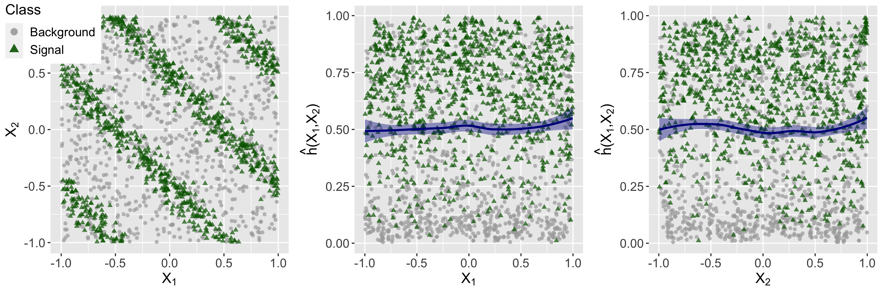
(a) $X_{1}$ versus $X_{2}$, $\widehat{h}(X_{1},X_{2})$ versus $X_{1}$ and $\widehat{h}(X_{1},X_{2})$ versus $X_{2}$

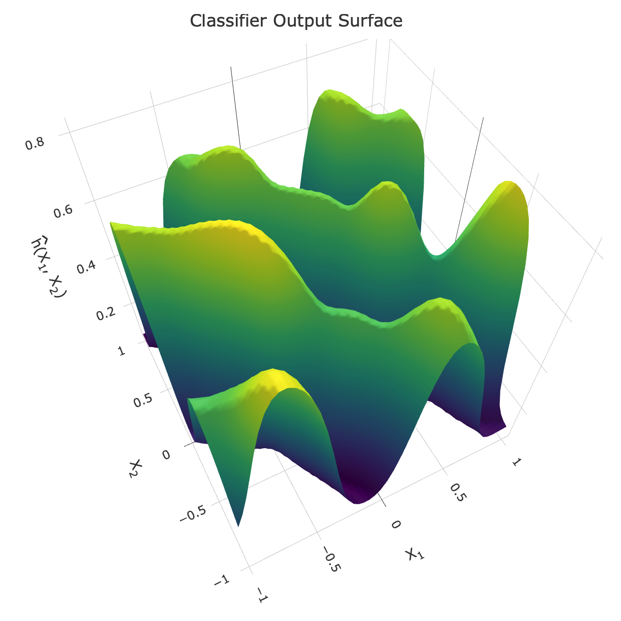
(b) Smoothed Classifier Surface

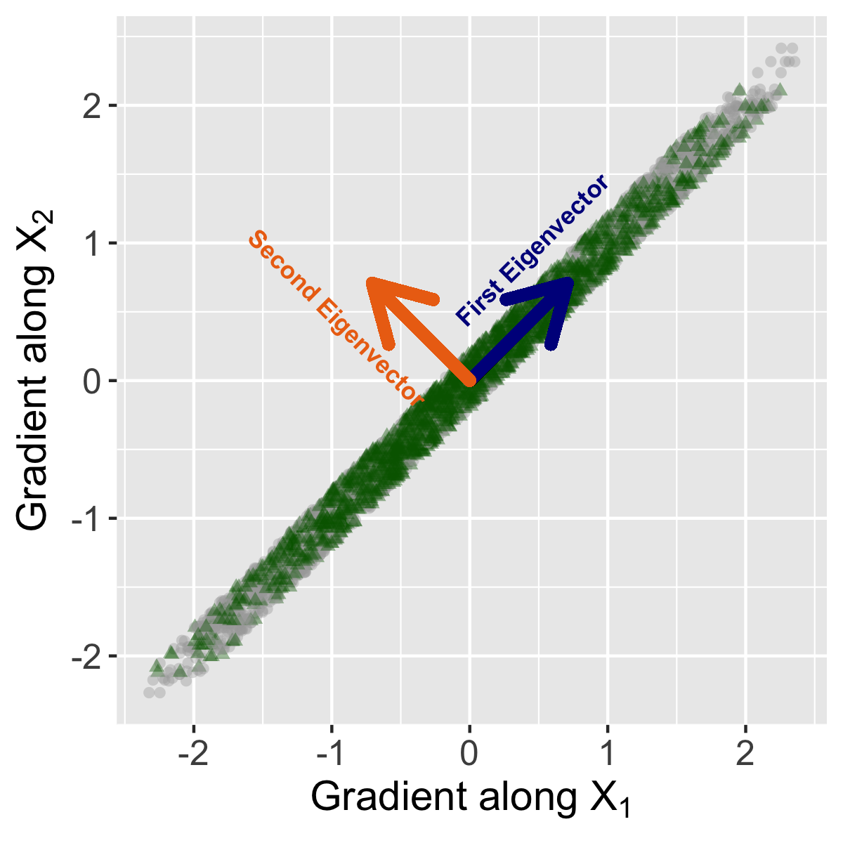
(c) PCA of the Standardized Gradients

Figure 3: We demonstrate the active subspace method on a two-dimensional example as shown in (a), where grey circles denote the uniformly distributed background and the green triangles denote the signal. The signal lies around lines parallel to the line $X_{1}+X_{2}=0$. Additionally, (a) also shows the output of the classifier that separates the signal from the background, $\widehat{h}(X_{1},X_{2})$, as a function of $X_{1}$ and $X_{2}$ individually. Neither of these variables marginally has separation power for the signal. (b) shows the smoothed classifier surface as a function of both $X_{1}$ and $X_{2}$. The active subspace method then performs PCA on the standardized gradients of the smoothed classifier output in (b). (c) shows a scatter plot of the standardized gradients of the smoothed classifier output as well as the two eigenvectors. We see that, as expected, the first eigenvector picks the direction in which the classifier output varies the most, namely $X_{1}-X_{2}=0$. We consider a two-dimensional example here for illustration purposes only. The real data can be of much higher dimensionality.

Figure 3 demonstrates the active subspace method on a two-dimensional example for simplicity, where the data $(X_{1},X_{2})\in[-1,1]\times[-1,1]$ and the signal lies around lines parallel to the line $X_{1}+X_{2}=0$. We then train a classifier $\widehat{h}(X_{1},X_{2})$ to separate the signal from the background. We notice that the classifier output does not appear to have any relationship with either $X_{1}$ or $X_{2}$ marginally, as shown in Figure 3(a). But the smoothed classifier surface detects the signal around lines parallel to the line $X_{1}+X_{2}=0$, as can be seen by the ridges along those lines in Figure 3(b). So, looking at the standardized gradients of the classifier surface gives us information about the direction in which the surface changes. As seen in Figure 3(c), the first eigenvector of the standardized gradients reflects the direction in which the classifier surface changes the most, which is along the $X_{1}-X_{2}=0$ line. Identifying this subspace helps us understand the directions in the feature space that separate the signal from the background. Note that we consider a two-dimensional example here for illustration purposes only. The real data can be of much higher dimensionality.

In what follows, instead of directly looking at the classifier $\widehat{h}(z)$, we look at $\text{logit}(\widehat{h}(z))=\log\left(\widehat{h}(z)/(1-\widehat{h}(z))\right)$. In practice for computational purposes, we add a small noise (e.g. $10^{-10}$) to $\widehat{h}(z)$ when $\widehat{h}(z)\in\{0,1\}$ to ensure that $\text{logit}(\widehat{h}(z))$ stays finite. We notice that taking the logit transformation provides more stable estimates of the gradients of the surface. Henceforth, we will instead look at the gradients of $H(z):=\text{logit}(\widehat{h}(z))$.

To find the gradient $\nabla_{z}H(z)$, we fit a local linear smoother to the logit of the random forest output. That is, we fit the logit of the classifier outputs $H(Z_{i})=\text{logit}(\widehat{h}(Z_{i}))$ locally around $z^{*}$ using

$$\widehat{H}(z)=\alpha(z^{*})+\beta(z^{*})^{T}(z-z^{*})+o\left(||z-z^{*}||_{2}^{2}\right).$$ (38)

Then, $\widehat{\beta}(Z_{i})$ provides estimates of the gradient of the logit classifier output on the data. We furthermore replace the gradient estimates $\widehat{\beta}_{j}(Z_{i})$ by their standardized versions $\widehat{\beta}_{j}(Z_{i})/sd(\widehat{\beta}_{j}(Z_{i}))$ at every data point $Z_{i}$, to get more stabilized values. So, henceforth $\widehat{\beta}(Z_{i})$ will be used to indicate the standardized gradient estimates for notational simplicity.

Remark.

The data used for estimating the gradient can either be the background data or the experimental data or a combination of both. We use a combination of both since experimentally we see that using the combination captures the classifier surface better.

We can then look at:

• The density of $\widehat{\beta}_{j}(Z)$, the estimated standardized gradient of $H(Z)$ along the $j^{th}$ variable.

• The active subspace found using the estimated standardized gradients $\widehat{\beta}(Z)$ as detailed in Section 5 below.

The density of $\widehat{\beta}_{j}(Z)$ explains how the classifier behaves marginally along each variable, whereas the active subspace identifies relationships between multiple variables that cause the most change in the classifier. We now describe the active subspace method in detail below.

5.1 Active Subspace of the Classifier

In this section we find the active subspace of the classifier $\widehat{h}$, which is assumed to be fixed and all the expectations in this section are with respect to the inputs of the fixed classifier. Let us consider the mean and the covariance matrix of $\nabla_{z}H(z)$. We define

$$C=\mbox{$\mathbb{E}$}_{f}\left[\left(\nabla_{z}H-\mbox{$\mathbb{E}$}\left[\nabla_{z}H\right]\right)\left(\nabla_{z}H-\mbox{$\mathbb{E}$}\left[\nabla_{z}H\right]\right)^{T}\right],$$ (39)

where $\mbox{$\mathbb{E}$}_{f}$ is the expectation with respect to the density $f=cp_{b}+(1-c)q$, where $c=m_{2}/(m_{2}+n_{2})$ gives the proportion of background data in the combined sample of background data $\mathcal{X}_{2}$ of size $m_{2}$ and experimental data $\mathcal{W}_{2}$ of size $n_{2}$ and $q=(1-\lambda)p_{b}+\lambda p_{s}$. We consider expectations with respect to $f$ since as explained in the remark above, we use a combination of the experimental data and the background data to find the active subspace of the classifier.

The mean $\mbox{$\mathbb{E}$}_{f}\left[\nabla_{z}H\right]$ gives the expected slope of the surface of $H(z)$. For example, a positive mean gradient along the $j^{th}$ variable indicates an increasing trend in the classifier output with that variable, meaning that increasing that variable increases the probability of an experimental data point and decreases the probability of a background data point. The covariance matrix $C$, on the other hand, encodes the variable relationships that cause variability in the classifier surface.

Consider the real eigenvalue decomposition of $C$,

$$C=M\Lambda M^{T},\ \ \ \Lambda=\text{diag}(\lambda_{1},\ldots,\lambda_{d}),\ \ \lambda_{1}\geq\ldots\geq\lambda_{d}\geq 0,$$ (40)

where $M$ has columns $\{{M}_{\cdot 1},\ldots,{M}_{\cdot d}\}$, the normalized eigenvectors of $C$. Then the vector ${M}_{\cdot 1}$ corresponding to $\lambda_{1}$, gives the association between the variables (i.e., the direction in the input space) that best captures the changes in $H(z)$ around the expected slope, followed by ${M}_{\cdot 2}$ and so on. Therefore the eigenvectors corresponding to the leading eigenvalues $\lambda_{1},\lambda_{2},\ldots$, give us an idea about the directions along which the classifier output changes the most. These are directions that contain meaningful information for separating the experimental data from the background data and therefore enable us to characterize how the experimental data differs from the background data. Towards this end, we propose Method 5.1 that uses the gradient estimates $\widehat{\beta}(Z)$ derived from a local linear smoother.

Method 5.1.

Active Subspace for the classifier $\widehat{h}$. 1. Split background data into ${\cal X}_{1}$ and ${\cal X}_{2}$ of sizes $m_{1}$ and $m_{2}$ respectively. Split experimental data into ${\cal W}_{1}$ and ${\cal W}_{2}$ of sizes $n_{1}$ and $n_{2}=m_{2}$ respectively. Train the classifier $\widehat{h}$ on ${\cal X}_{1}$ and ${\cal W}_{1}$. 2. Fit a local linear smoother that estimates $H(Z_{i})=\text{logit}\left(\widehat{h}(Z_{i})\right)$ for $Z_{i}\in{\cal X}_{2}\cup{\cal W}_{2}$ using the model given in (38). 3. Consider the coefficients of the local linear smoother $\widehat{\beta}(Z_{i})$ for $Z_{i}\in{\cal X}_{2}\cup{\cal W}_{2}$. They provide an estimate of the gradient $\nabla_{z}H$ at $Z_{i}$, i.e., $\widehat{\nabla_{z}H(Z_{i})}=\widehat{\beta}(Z_{i})$ for $Z_{i}\in{\cal X}_{2}\cup{\cal W}_{2}$. 4. Standardize the estimated gradients $\widehat{\beta}_{j}(Z_{i})$ to $\widehat{\beta}_{j}(Z_{i})/\widehat{sd(\widehat{\beta}_{j}(Z_{i}))}$ by using the estimated $\widehat{sd(\widehat{\beta}_{j}(Z_{i}))}$ given by the local linear smoother. 5. Then instead of $C$ we can use the estimate $$\widehat{C}=\frac{1}{N}\sum_{Z_{j}\in{\cal X}_{2}\cup{\cal W}_{2}}\left(\widehat{\beta}(Z_{j})-\overline{\widehat{\beta}(Z)}\right)\left(\widehat{\beta}(Z_{j})-\overline{\widehat{\beta}(Z)}\right)^{T},$$ (41) where $\overline{\widehat{\beta}(Z)}=\sum_{Z_{j}\in{\cal X}_{2}\cup{\cal W}_{2}}\widehat{\beta}(Z_{j})/N$ and $N=m_{2}+n_{2}$. 6. Find the eigenvalue decomposition of $\widehat{C}$ as $$\widehat{C}=\widehat{M}\widehat{\Lambda}\widehat{M}^{T},$$ which gives the estimates $\widehat{M}$ and $\widehat{\Lambda}$ of $M$ and $\Lambda$ as defined in (40) respectively. We find the eigenvectors by performing PCA on the standardized gradients. 7. Then $\overline{\widehat{\beta}(Z)}$ and the estimated eigenvectors $\widehat{M}_{\cdot 1},\widehat{M}_{\cdot 2},\ldots$ given by the columns of $\widehat{M}$, best capture the slope and variations in $H(\cdot)$ and hence the classifier surface, respectively.

We can additionally construct bootstrapped uncertainty intervals by repeatedly drawing with replacement $m_{b}$ background samples from ${\cal X}$ and $n$ experimental samples from ${\cal W}$ and split them into ${\cal X}_{1}^{*}$, ${\cal X}_{2}^{*}$, ${\cal W}_{1}^{*}$ and ${\cal W}_{2}^{*}$ of sizes $m_{1},m_{2},n_{1}$ and $n_{2}$ at random ensuring no overlap between the training and test data sets. That is, ${\cal X}_{1}^{*}\cap{\cal X}_{2}^{*}=\phi$ and ${\cal W}_{1}^{*}\cap{\cal W}_{2}^{*}=\phi$. In each case, we first re-train the classifier on the new training data ${\cal X}_{1}^{*}\cup{\cal W}_{1}^{*}$ and then find $\overline{\widehat{\beta}(Z)}$, and the estimated eigen values $\widehat{M}_{\cdot 1},\widehat{M}_{\cdot 2},\ldots$ on the new test data ${\cal X}_{2}^{*}\cup{\cal W}_{2}^{*}$. Here $m_{1},m_{2},n_{1}$ and $n_{2}$ are the same as in Method 5.1. We can then use the standard deviation or quantiles of the bootstrapped estimates to create bootstrap confidence intervals that will give estimates of the stability of the estimators, given by the algorithm, to perturbations in the data.

6 Experiments: Search for the Higgs Boson

We demonstrate the performance of the proposed semi-supervised classifier tests on the Higgs boson machine learning challenge data set available on the CERN Open Data Portal at http://opendata.cern.ch/record/328 (ATLAS Collaboration, 2014). The data set consists of simulated data provided by the ATLAS experiment at CERN’s Large Hadron Collider to optimize the search for the Higgs boson.

Our goal is to demonstrate the performance of the proposed tests in identifying the presence of the Higgs boson particle without assuming an a priori ansatz of the signal and demonstrate their applicability to model-independent searches of new physics signals in experimental particle physics.

6.1 Data Description

The Higgs boson has many different ways through which it can decay in an experiment and produce other particles. This particular challenge, from which our data set originates, focuses on the collision events where the Higgs boson decays into two tau particles (Adam-Bourdarios et al., 2015). The data provided for the challenge consist of collision events labelled as background and signal. The signal class is comprised of events in which a Higgs boson (with a fixed mass of 125 GeV) was produced and then decayed into two taus. The events are simulated using the official ATLAS full detector simulator. The simulator yields simulated events with properties that mimic the statistical properties of the real events of the signal type as well as several important backgrounds. For the sake of simplicity, background events generated from only three different background processes were included in the challenge data set. Our objective is to show that semi-supervised classifier tests are able to identify the Higgs signal without any prior knowledge.

The data set has 818,238 observations, where each observation is a simulated proton-proton collision event in the detector. Each of these collision events produces clustered showers of hadrons, which originate from a quark or a gluon produced during the collision. These showers are called jets. The data contain information on the measured properties of the jets as well as the other particles produced during the collision. There are $d=35$ features whose individual details can be found on CERN’s Open Data Portal or in Appendix B of Adam-Bourdarios et al. (2015). Here we give some insight into the most important characteristics of the features.

The features whose names start with PRI are primitive variables that record the raw quantities as measured by the detector. The features whose names start with DER are derived variables which are evaluated as functions of the primitive variables. Since all collision events do not produce the same number of jets, the number of jets produced in the collisions, denoted by PRI_jet_num, ranges from $0-3$ (events with more than $3$ jets are capped at $3$). Note that it is possible for the collisons to not produce any jets (PRI_jet_num$=0$) and hence there are structurally absent missing values in the data that relate to the jets produced in the collisions. To avoid these missing values in the data, we only consider events that have two jets (PRI_jet_num$=2$). This results in 165,027 events; 80,806 background events and 84,221 signal events. Since the derived quantities are functions of the primitives, we use just the primitive variables ($d=16$) for our analysis. Since we only use the primitive variables, we drop the pre-fix PRI from the variable names and further shorten some of the variable names intuitively for convenience. Descriptions of the primitive variables used are provided in Table 2.

Among the primitive features, five of them provide the azimuth angle $\phi$ of the particles generated in the event (variables ending with _phi). These features are rotation invariant in the sense that the event does not change if all of them are rotated together by the same angle. Hence to interpret these variables more easily using the active subspace method, we remove the invariance of the azimuth angle variables by rotating all the $\phi$’s so that the azimuth angle of the leading jet at $0$ (lead_phi$=0$). lead_phi can then be removed from the analysis, leading to a 15-dimensional feature space.

Table 2: Descriptions of the variables used in the analysis of the Higgs boson machine learning challenge data set (Adam-Bourdarios et al., 2015). We drop the pre-fix PRI from the variable names and further shorten some of the variable names intuitively for convenience.

Variable	Description
tau_pt	The transverse momentum of the hadronic tau.
tau_eta	The pseudorapidity $\eta$ of the hadronic tau.
tau_phi	The azimuth angle $\phi$ of the hadronic tau.
lep_pt	The transverse momentum of the lepton (electron or muon).
lep_eta	The pseudorapidity $\eta$ of the lepton.
lep_phi	The azimuth angle $\phi$ of the lepton.
met	The missing transverse energy.
met_phi	The azimuth angle $\phi$ of the missing transverse energy.
met_sumet	The total transverse energy in the detector.
lead_pt	The transverse momentum of the leading jet, i.e., the jet with the largest transverse momentum (undefined if PRI_jet_num $=0$).
lead_eta	The pseudorapidity $\eta$ of the leading jet (undefined if PRI_jet_num $=0$).
lead_phi	The azimuth angle $\phi$ of the leading jet (undefined if PRI_jet_num $=0$).
sublead_pt	The transverse momentum of the subleading jet, i.e., the jet with the second largest transverse momentum (undefined if PRI_jet_num $\leq 1$).
sublead_eta	The pseudorapidity $\eta$ of the subleading jet (undefined if PRI_jet_num $\leq 1$).
sublead_phi	The azimuth angle $\phi$ of the subleading jet (undefined if PRI_jet_num $\leq 1$).
all_pt	The scalar sum of the transverse momentum of all the jets in the event.
Weight	The event weight.
Label	The event label (string) (s for signal, b for background).

Additionally, we take logarithmic transformations of the variables that give the transverse momentum of the particles produced (variables ending with _pt), the missing transverse energy (met) and the total transverse energy in the detector (met_sumet). Exploratory analysis of the data as well as details and justifications for the transformations considered above, can be found in the Supplementary Material (Chakravarti et al., 2022).

Experimental Setting: In all the following experiments on the Higgs boson data set, we randomly sample without replacement background and signal events from the original data set to form background data with $m_{b}=$ 40,403 events, signal data with $m_{s}=$ 20,403 events, and experimental data with $n=$ 40,403 events. In this manner we generate 50 replicates of each of these data sets for use in our power studies.

Recall that the experimental data is a mixture of background and signal data, where the proportion of signal data is given by $\lambda$, the signal strength. So, the number of signal events in the experimental data is decided according to $\lambda$ by randomly generating from Bin$(n,\lambda)$. For methods that require data-splitting, the data-splitting is done by randomly splitting the background data into $m_{1}=$ 20,403 training and $m_{2}=$20,000 test background samples and by randomly splitting the experimental data into $n_{1}=$20,403 training and $n_{2}=$20,000 test experimental samples. We construct the splits so the number of signal events in the training and test experimental samples are randomly generated from Bin$(n_{1},\lambda)$ and Bin$(n_{2},\lambda)$, respectively. Additionally, when randomly generating the experimental data, events are selected in a weighted fashion using the Weight variable provided in the data set as described in Table 2. Note that the classifiers for the model-dependent approaches are trained on $m_{1}=$ 20,403 background and $m_{s}=$ 20,403 signal training samples, and the classifiers for the model-independent approaches are trained on $m_{1}=$ 20,403 background and $n_{1}=$ 20,403 experimental training samples. Hence, all the classifiers are trained on balanced datasets. For each of the bootstrap and permutation methods we consider 1,000 bootstrap and permutation cycles respectively.

In the following sections, we first explore the power of the classifier tests described in Section 3 to detect the presence of the Higgs boson signal in the experimental data. We then estimate the signal strength ($\lambda$) using the methods introduced in Section 4 and then use the active subspace method introduced in Section 5 to characterize the signal. All the code used for this section is available at https://github.com/purvashac/MIDetectionClassifierTests.

6.2 Anomaly Detection Using the Classifier Tests

We compare the power of the model-dependent supervised methods and the model-independent semi-supervised methods introduced in Section 3 in detecting the Higgs boson signal, by varying the signal strength from $\lambda=0.15$ to $\lambda=0.01$. We also check that the tests have the right error control under the null case ($\lambda=0$). We demonstrate the performance of the different methods – asymptotic, bootstrap, permutation (using out-of-sample statistics), and slow permutation (using in-sample statistics), used along with the different test statistics – Likelihood Ratio Test statistic (LRT), Score statistic, Area Under the Curve (AUC), and Misclassification Error (MCE).

For the model-dependent methods, since we have only finitely many samples from the background available, and not the background generator itself, we split the available background data into training and test sets as described above. We then use the training set for fitting the classifier and the test set for estimating the null distribution of the test statistic by bootstrapping or permuting as described in Section 3. In real life, since the background MC generator is known, we should, in many cases, be able to generate more training background samples for estimating the null distribution of the test statistic.

6.2.1 Anomaly Detection when Data has a Correctly Specified Signal

We first compare the methods when the signal model is correctly specified. The tests are run on $50$ random samplings of the data, and the percentage of times each of the tests rejects the null that there is no signal, is given in Table 3. “Permutation” indicates the faster permutation method from Section 3.2, that uses out-of sample test statistics for testing, and “Slow Perm” indicates the slower permutation method from Section 3.2 that uses in-sample test statistics for testing and re-trains the classifier in every permutation cycle. The significance level for all the tests is considered at $\alpha=0.05$.

Table 3: Power of detecting the signal in the Higgs boson data for each method in percentages. We consider 50 random samplings of the data and 1,000 bootstrap and permutation cycles. We perform each test at $\alpha=5\%$ significance level. The last column ($\lambda=0$) represents the Type I error of the methods.

		Signal Strength ($\lambda$)
Model	Method	$0.15$	$0.1$	$0.07$	$0.05$	$0.03$	$0.01$	$0$
Supervised LRT	Asymptotic	100	100	96	62	18	18	6
	Bootstrap	100	96	78	58	6	0	0
	Permutation	100	98	98	86	28	6	0
Supervised Score	Bootstrap	64	66	74	50	18	0	0
	Permutation	94	92	100	92	80	24	12
Semi-Supervised LRT	Asymptotic	100	98	74	38	16	6	2
	Bootstrap	100	98	48	10	2	2	0
	Permutation	100	98	72	38	16	6	2
	Slow Perm	82	8	0	4	2	0	4
Semi-Supervised AUC	Asymptotic	100	96	78	32	14	4	2
	Bootstrap	100	98	70	32	20	6	2
	Permutation	100	98	68	32	20	4	2
	Slow Perm	100	100	94	56	20	8	4
Semi-Supervised MCE	Asymptotic	100	92	60	28	14	2	2
	Bootstrap	100	96	52	28	16	6	4
	Permutation	100	96	52	30	14	6	6
	Slow Perm	100	98	86	58	16	6	2

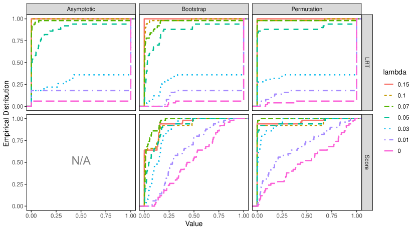
Figure 4: Empirical CDF of the p-values given by the supervised tests for different signal strengths ($\lambda$). The columns in the grid of plots represent the different methods of testing (asymptotic, bootstrap and permutation) and the rows represent the use of the different test statistics (LRT and Score). Note that the plot for the asymptotic test using the score statistic is missing since we do not consider that test due to the poor quality of the asymptotic approximation.

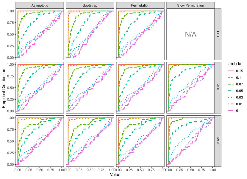
Figure 5: Empirical CDF of the p-values given by the semi-supervised tests for different signal strengths ($\lambda$). The columns in the grid of plots represent the different methods of testing (asymptotic, bootstrap, permutation and slow permutation) and the rows represent the use of the different test statistics (LRT, AUC and MCE). We leave out the plot for slow permutation test using the LRT statistic since in practice it demonstrates very poor performance. It suffers from bias caused by over-fitting since for slow permutation we consider the in-sample LRT.

As seen in Table 3, among the supervised methods, the permutation tests out-perform all the other supervised methods in terms of power. The permutation test with the score statistic has the most power for smaller values of $\lambda$. However, it is worth noting that it might be anticonservative for $\lambda=0$ and hence, might not have the right significance level. Conversely, as Table 3 and Figure 4 show, the supervised tests that use the LRT statistic appear to be overly conservative for smaller values of $\lambda$, because the LRT statistic uses an estimate of the density ratio $p_{s}/p_{b}$ using the classifier. This problem mainly appears when two conditions are both in effect: (1) the classifier for background versus signal overfits the class probabilities, by overfitting to the data, and (2) when $\lambda=0$; i.e., when the experimental data has no signal. Under this situaton, then, with probability higher than expected, almost the entire experimental data is classified as background with $\widehat{h}({Z_{i}})=0$, and $\widehat{p_{s}/p_{b}}=0$. This makes $\widehat{\lambda}_{\text{MLE}}$, the maximum likelihood estimator of $\lambda$, also zero, making the LRT statistic zero as well. This is also observed when we use the permutation or bootstrap methods to estimate the null distribution. The estimated distributions have a point mass at zero that is much higher than $0.5$ (as given by the asymptotic distribution in Equation (15) when true $p_{s}/p_{b}$ is used). Note that we additionally leave out the asymptotic score test both in Table 3 and Figure 4 since we tried the test for a sub-sample of the data and decided to not consider that test for the larger data set due to the poor quality of the asymptotic approximation.

Among the semi-supervised approaches, the AUC and MCE slow permutation methods (slow perm) have power that is only slightly worse than that of the supervised methods, as shown in Table 3. Importantly, the semi-supervised methods achieve this without having access to the labeled signal sample during training. Among the asymptotic and the faster permutation methods, using LRT or MCE gives similar performance to AUC in the semi-supervised approaches. We also observe that the slow permutation method using the LRT statistic has very low power. This is due to bias in estimating the LRT using an in-sample estimate which is influenced by over-fitting.

Figure 5 shows the empirical distributions of the $p$-values produced by the semi-supervised tests for different $\lambda$ values. All the tests appear to have correct (or at least almost correct) type I error control as indicated by the close to uniform CDFs in the $\lambda=0$ case. We also notice that none of the tests have much power to detect signals that are less than $3\%$ of the experimental data $(\lambda<0.03)$. We omit the plot for the slow permutation method using the LRT as it has anomalously low power for most $\lambda$ values due to the reasons mentioned above.

We additionally compared these methods to nearest neighbor (NN) two-sample tests as introduced in Schilling (1986) and Henze (1988). We considered the nearest neighbor tests as opposed to other tests, since the signal that we are trying to detect, appears as a collection of nearby data points. Hence tests based on neighborhoods should have better power to detect it. We compared the methods presented in this paper to the NN tests (asymptotic and permutation versions) for a sub-sample of the data set. We observed that the asymptotic version especially had very poor power. The permutation version performed better, but was out-performed by the semi-supervised AUC, MCE and LRT methods. Additionally, it was not scalable to extend it to the larger data set. Hence we concluded that it was computationally impractical to apply it to the larger full data set.

In conclusion, we see that slow permutation method when using the AUC and MCE statistics out-performs the other semi-supervised methods and additionally gives comparable performance to the supervised methods in detecting the signal in the experimental data. Note that the power of the slow permutation method using the AUC and MCE statistics is much better than the one using the LRT statistic, which is the statistic used by D’Agnolo and Wulzer (2019) and D’Agnolo et al. (2021). So these methods give an improvement over using just the LRT statistic.

6.2.2 Anomaly Detection when Data has a Misspecified Signal

As mentioned in the introduction, a model-dependent search that targets one kind of new physics signal will not be powerful to detect a different signal which might actually be present in the data. This is one of the main motivations for model-independent methods. In this section, we demonstrate that if the signal model is misspecified in just one dimension, model-independent methods are still able to detect the signal, whereas the model-dependent methods fail to detect the signal.

We transform the signal in the experimental data to intentionally make it different from the signal model, which makes the signal model misspecified. We consider a transformation in just one variable, transforming

$$\verb!tau_pt!^{*}=\verb!tau_pt!-0.7\ \left(\verb!tau_pt!-\min(\verb!tau_pt!)\right).$$ (42)

in the experimental data. Meanwhile, we do not transform the signal data used by the supervised methods for training the classifier. This simulates a misspecified signal situation, where the signal in the experimental data is not from the same distribution as the signal used by the supervised methods for training. This is to emulate a situation where the signal in the experimental data is different from the signal that the signal model specifies in just one dimension.

We chose this particular transformation for multiple reasons. First, it transforms the variable that has the most marginally different means for the background and the signal data as demonstrated by Figure 4 in the Supplementary Material (Chakravarti et al., 2022). Second, the marginal distribution of the signal along this variable is different from the marginal distribution of the background. These two reasons make tau_pt a variable that potentially influences the classifier. By transforming the variable, we lower the mean tau_pt for the signal in the experimental data, causing the model dependent methods to lose power in detecting the transformed signal.

We now compare the power of the supervised and the semi-supervised methods in detecting the transformed signal in the experimental data. The tests are run on $50$ random samplings of the data, and the percentage of times each of the tests rejects the null that there is no signal, is given in Table 4. As before, “Permutation” indicates the faster permutation method from Section 3.2, that uses out-of-sample test statistics for testing and “Slow Perm” indicates the slower permutation method from Section 3.2, that uses in-sample test statistics for testing and re-trains the classifier in every permutation cycle. The significance level for all the tests is considered at $\alpha=0.05$.

Table 4: Power of detecting the misspecified signal in the Higgs boson data for each model in percentages. We consider 50 random samplings of the data and 1,000 bootstrap and permutation cycles. We perform each test at $\alpha=5\%$ significance level. The last column ($\lambda=0$) represents the Type I error of the methods.

		Signal Strength ($\lambda$)
Model	Method	$0.15$	$0.1$	$0.07$	$0.05$	$0.03$	$0.01$	$0$
Supervised LRT	Asymptotic	2	10	2	8	8	6	4
	Bootstrap	0	0	0	0	0	0	0
	Permutation	0	0	0	0	0	2	0
Supervised Score	Bootstrap	0	0	0	0	0	0	0
	Permutation	0	0	0	0	0	2	8
Semi-Supervised LRT	Asymptotic	100	100	100	82	18	4	4
	Bootstrap	100	100	100	60	4	2	0
	Permutation	100	100	100	82	18	4	2
	Slow Perm	100	100	78	22	2	4	6
Semi-Supervised AUC	Asymptotic	100	100	100	78	16	8	4
	Bootstrap	100	100	100	82	20	10	0
	Permutation	100	100	100	80	20	8	2
	Slow Perm	100	100	100	100	34	10	4
Semi-Supervised MCE	Asymptotic	100	100	100	66	24	6	4
	Bootstrap	100	100	100	62	16	6	4
	Permutation	100	100	100	62	14	6	4
	Slow Perm	100	100	100	98	22	8	2

As seen in Table 4, as expected, the supervised methods have no power at all in detecting the transformed signal. An interesting observation from the table is that, it appears that the supervised methods are more conservative when there is some signal present compared to when there is no signal present. This occurs as the signal labels that the supervised models are trained on are inconsistent with the signal in the experimental data, when the signal is present.

The semi-supervised methods on the other hand, still have power to detect the transformed signal since they are not trained on the misspecified signal training data. In fact, the semi-supervised methods appear to have higher power with the transformed signal than with the original signal, indicating that the transformed signal is somewhat easier to disentangle from the background than the original signal. Comparing the semi-supervised methods, we again observe that the slow permutation method using AUC has the highest power. We also notice that the asymptotic and permutation tests that use LRT demonstrate power comparable to the AUC. The slow permutation method with MCE also performs comparably to the slow permutation method with AUC. The slow permutation method with LRT has again anomalously low power for smaller $\lambda$, due to the bias caused by using the in-sample LRT as the test statistic.

In conclusion, semi-supervised methods continue to demonstrate power similar to the previous case where the signal model was not misspecified. On the other hand, the supervised models do not have any power to detect the transformed signal in the misspecified model case, which motivates the use of semi-supervised models in such a case.

6.2.3 Anomaly Detection with Smaller Signal Strengths

So far, the signal strengths that we have considered in this paper have been in the order of $10^{-2}$ and the sample sizes have been in the order of $10^{4}$. But, in many high-energy physics searches, the signal strengths that the physicists are looking for are in the order of $10^{-3}-10^{-4}$ and they have much larger sample sizes as well. For example, the true signal strength of the Higgs Boson signal in the data set where the two jets are produced is $\lambda=0.0035$. In this section, we show that the power of the model-independent methods to detect signal for smaller signal strengths increases as the sample size increases.

We perform the asymptotic model-independent tests on equally sized background and experimental data sets whose sample sizes vary from $2\times 10^{4}$ to $2\times 10^{6}$, with signal strengths $\lambda$ varying from $0.001-0.05$. To make this experiment feasible (due to the lack of availability of sufficient background samples in our original data set), we fit a mixture of 8 multivariate Normals to the background data and a mixture of 9 multivariate Normals to the signal data in the Higgs boson data set. We then generate samples from the estimated mixtures of Normals to create our simulated data sets for this experiment.

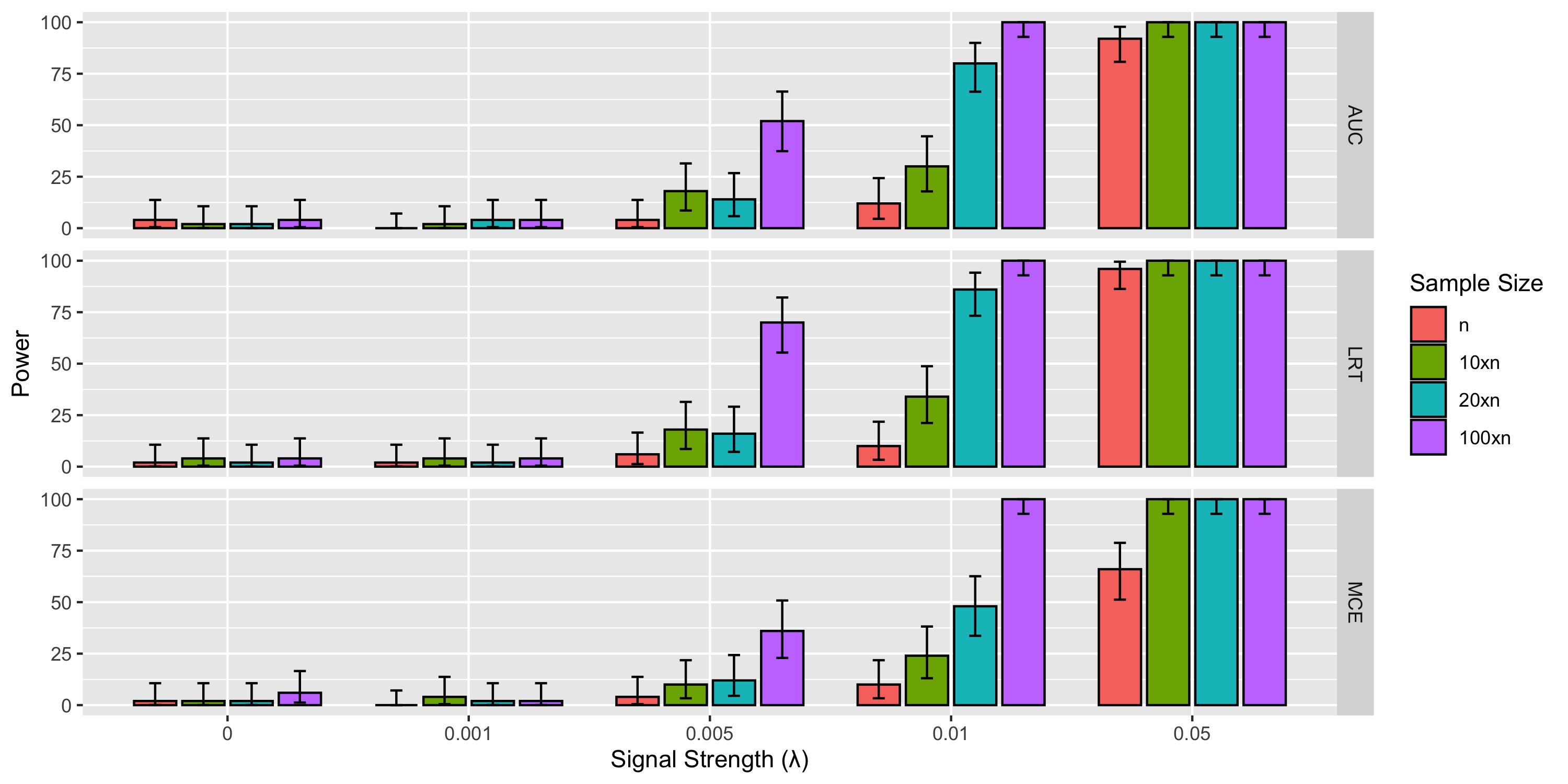
Figure 6: Power of the asymptotic model-independent tests using AUC, LRT, and MCE statistics to detect different signal strengths ($\lambda=0,0.001,0.005,0.01,0.05$) in 50 simulations with samples of sizes $n,10n,20n,$ and $100n$, where $n=2\times 10^{4}$. $\lambda=0$ represents the Type I error rate. The error bars represent the $95\%$ Clopper-Pearson confidence intervals for the power. We note that for all the three statistics, the power increases in larger sized samples for $\lambda=0.005,0.01,0.05$. For $\lambda=0.001$, none of the tests appear to have power to detect the signal, but further increases in the sample size should provide power in this case as well.

Figure 6 shows that for smaller signal strengths, for, e.g., $\lambda=0.005$, the power of the model-independent tests increases as the sample size increases. We see that for the largest sample size, $100n=2\times 10^{6}$, the model-independent tests have good power even for $\lambda=0.005$, which is comparable to the true Higgs Boson signal strength ($0.0035$) in the two jets channel. Whereas, for the sample size that we used in our previous experiments, $n=2\times 10^{4}$, the model-independent tests have small power for $\lambda=0.01$ and no power for $\lambda=0.005$. This demonstrates that when larger data sets are available, the model-independent methods have power to detect even smaller signal strengths. In many search channels, LHC data sets are of the order of millions or billions of events, so these tests should have power for detecting reasonably small signals in those channels.

6.3 Estimating the Higgs Boson Signal Strength

In this section, we demonstrate the performance of the methods proposed in Section 4 to estimate the signal strength ($\lambda$) using the Higgs boson data set. We vary the signal strength from $\lambda=0.5$ to $\lambda=0$ and look at the estimates of the signal strength as well as the bootstrapped uncertainty intervals given by Method 4.1 in Section 4.

We consider $100$ bootstrap cycles to get the $95\%$ bootstrapped uncertainty intervals. For the estimates, we consider $T\in\{0.8,0.5\}$ and $b\in\{0.01,0.005\}$, where $T$ is the threshold that indicates the neighborhood of $1$ where we fit the Poisson regression model and $b$ is the bin-width of the histogram that we use to estimate the densities. Note that bin-width $b\in\{0.01,0.005\}$ is equivalent to the number of bins, Bins $\in\{100,200\}$. To construct the bootstrapped uncertainty intervals, we use three different methods using $\alpha=5\%$ and compare them in Figure 7 below.

First, we use the basic bootstrap confidence interval, also known as the Reverse Percentile Interval, which uses empirical quantiles of the bootstrap distribution of $\widehat{\lambda}$ in a reverse order to construct the confidence interval (see Davison and Hinkley (1997), Eq. (5.6), p. 194): $(2{\widehat{\lambda\,}}-\lambda_{(1-\alpha/2)}^{*},2{\widehat{\lambda\,}}-\lambda_{(\alpha/2)}^{*})$, where $\lambda_{(1-\alpha/2)}^{*}$ denotes the $1-\alpha/2$ quantile of the bootstrapped estimates $\lambda^{*}$.

Second, we use the bootstrapped quantiles to form percentile bootstrap confidence intervals (see Davison and Hinkley (1997), Eq. (5.18), p. 203, Efron and Tibshirani (1994), Eq. (13.5), p. 171): $(\lambda_{(\alpha/2)}^{*},\lambda_{(1-\alpha/2)}^{*})$.

Third, we use bootstrapped standard errors and normal distribution’s quantiles to create bootstrap confidence intervals: $(\widehat{\lambda}-z_{1-\alpha/2}\ {\widehat{\text{se}}}_{\lambda^{*}},\widehat{\lambda}+z_{1-\alpha/2}\ {\widehat{\text{se}}}_{\lambda^{*}})$ where $z_{1-\alpha/2}$ denotes the $1-\alpha/2$ quantile of the standard normal distribution, and ${\widehat{\text{se}}}_{\lambda^{*}}$ is the standard error estimated using the empirical standard deviation of the bootstrapped estimates $\lambda^{*}$.

We additionally present the confidence intervals given by the GLM model (Dobson and Barnett, 2018) itself in Figure 7.

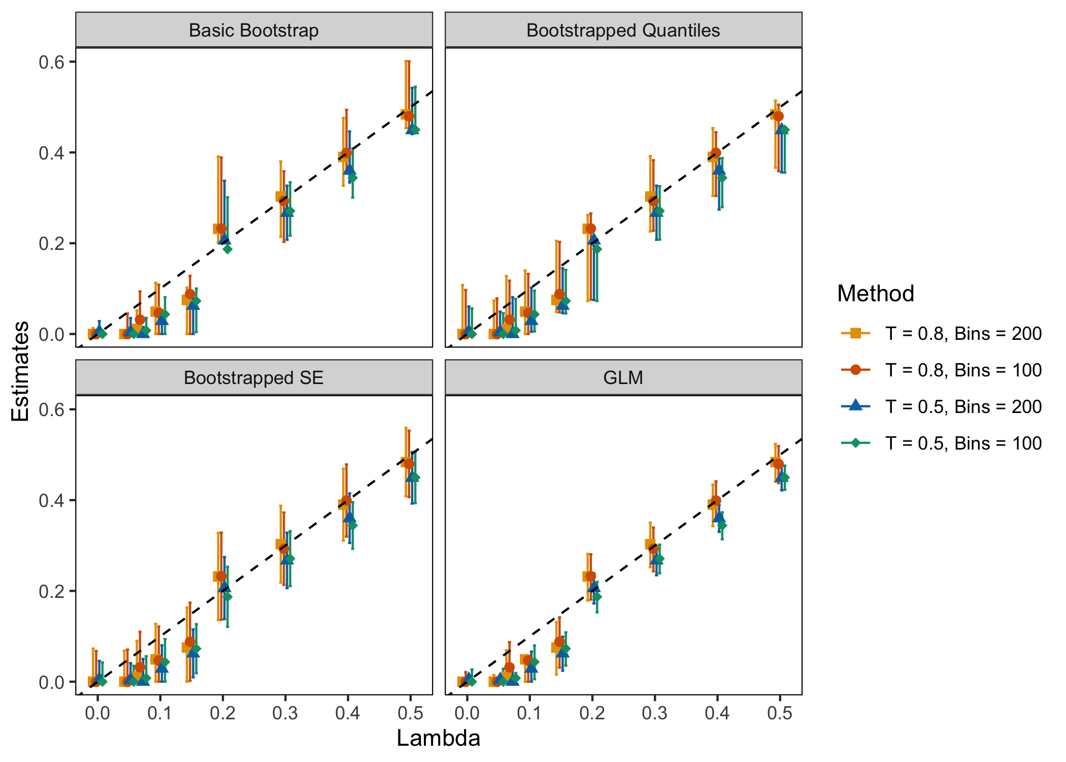
Figure 7: Estimates of the signal strength ($\lambda$), along with the $95\%$ uncertainty intervals, of the Higgs boson in the experimental data. The true $\lambda$, given by the dotted diagonal line, varies from $0$ to $0.5$. $T$ specifies the threshold that controls the size of the neighborhood of $1$ that is considered in the Poisson regression model and Bins specifies the number of bins considered in the histogram when estimating the density of $\widehat{g_{q}}(1)$ as described in Section 4.

We observe from Figure 7 that the estimates of $\lambda$ do not vary much with the number of bins used for the histogram estimate of the density. We also notice that thresholding at $T=0.8$ which is closer to $1$ as compared to $T=0.5$, gives better estimates of $\lambda$. We additionally tried $T=0.9$ on a sub-sample of the data set. But the estimates in that case were not very stable and hence, we decided to not consider them for the final larger data set. The uncertainty intervals created using bootstrapped quantiles and bootstrapped standard errors appear to be relatively well-calibrated when $T=0.8$, i.e., they include the true value of $\lambda$, given by the dotted diagonal line, in each of the plots. The uncertainty intervals given by the GLM model and basic bootstrap, on the other hand, do not contain the true $\lambda$ for some smaller values of $\lambda$. So, $\widehat{\lambda}$ using $T=0.8$ with the number of bins either $100$ or $200$, accompanied with either bootstrapped quantile or bootstrapped standard error uncertainty intervals, appears to give the best performance in estimating and quantifying the uncertainty of the signal strength $\lambda$. An additional advantage of the uncertainty intervals using bootstrapped standard errors is that they are centered about the estimate $\widehat{\lambda}$.

6.4 Interpreting the Classifier Using Active Subspace Methods

We demonstrate the application of the active subspace methods for a random simulation (one of the 50 simulations in Section 6.2) which detects the signal at significance level $\alpha=0.05$, when $\lambda=0.15$, i.e., $15\%$ of the experimental data is from the signal sample. We consider $\lambda=0.15$, since the random forests demonstrate good power in detecting the signal for that signal strength (Table 3).

We then use Method 5.1 presented in Section 5 to find the active subspace of the fitted semi-supervised classifier. The second step of the algorithm requires us to choose a linear smoother as well as a smoothing parameter for it. We choose a Gaussian kernel smoother as the linear smoother and $h=0.5$ as the smoothing parameter. The smoothing parameter $h$ is used to scale the standard deviations of the variables, which is then used as the standard deviation of the multivariate Gaussian kernel, i.e., $\widehat{sd}(Z)/h$ is considered as the standard deviation of the multivariate Gaussian kernel. The smoothing parameter selection process is described in the Supplementary Material (Chakravarti et al., 2022).

Figure 8 gives us the active variables given by the mean standardized gradient, the first eigenvector and the second eigenvector. The higher eigenvectors do not contain much information and have been included in the Supplementary Material (Chakravarti et al., 2022). The figure additionally gives the distribution of the bootstrapped active subspace estimates as violin plots. These help us construct $95\%$ uncertainty intervals for the active subspace variables using the bootstrapped empirical percentiles. We consider $500$ bootstrap cycles to get the $95\%$ bootstrapped uncertainty intervals.

Figure 8(a) additionally provides the violin plots of the standardized gradient estimates $\widehat{\beta}_{j}(Z_{i})/\widehat{sd(\widehat{\beta}_{j}(Z_{i}))}$ given by the local linear smoother at every point in the combined test data $Z_{i}\in\mathcal{X}_{2}\cup\mathcal{W}_{2}$. We notice that the violin plots are not very informative since they are all symmetric about zero, i.e., they don’t appear to give any information about the slope of the classifier surface.

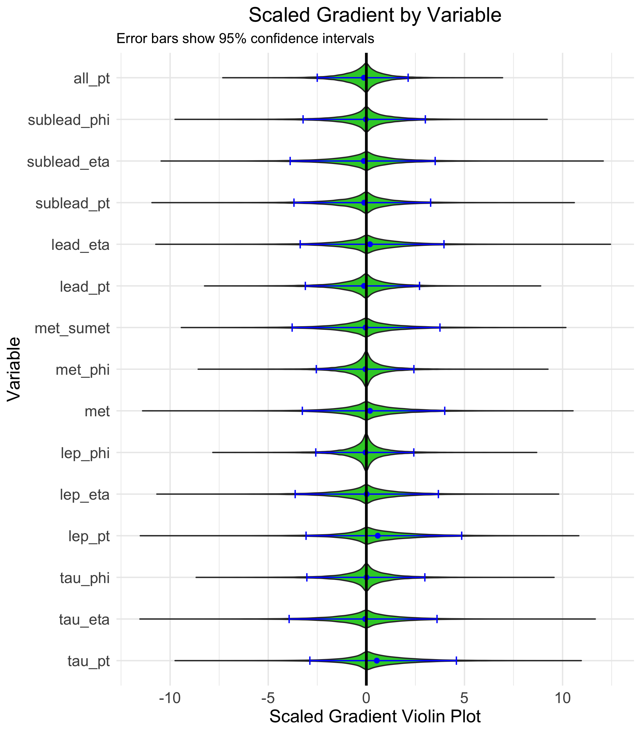
(a) Standardized Gradient Distribution

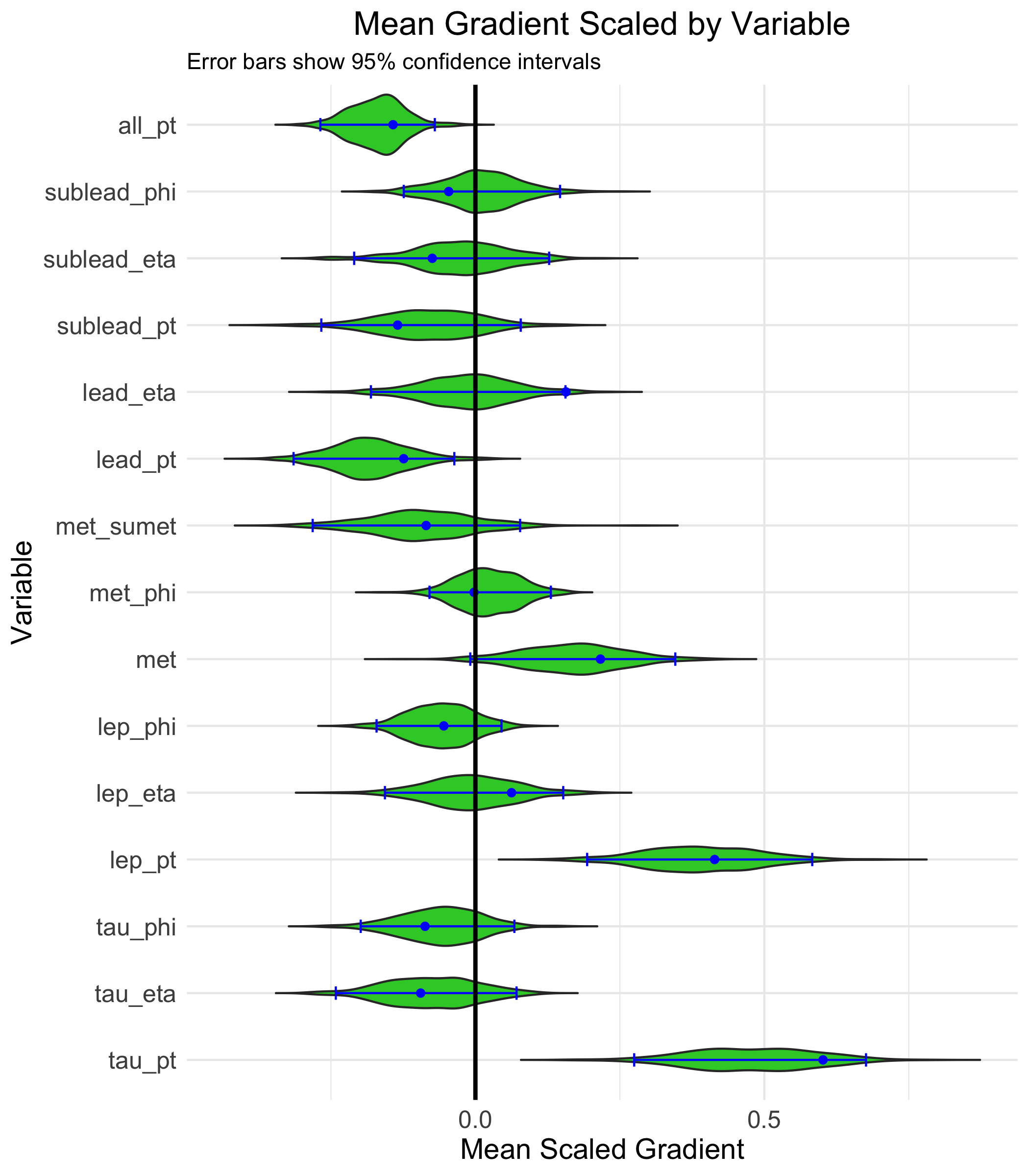
(b) Mean Standardized Gradient

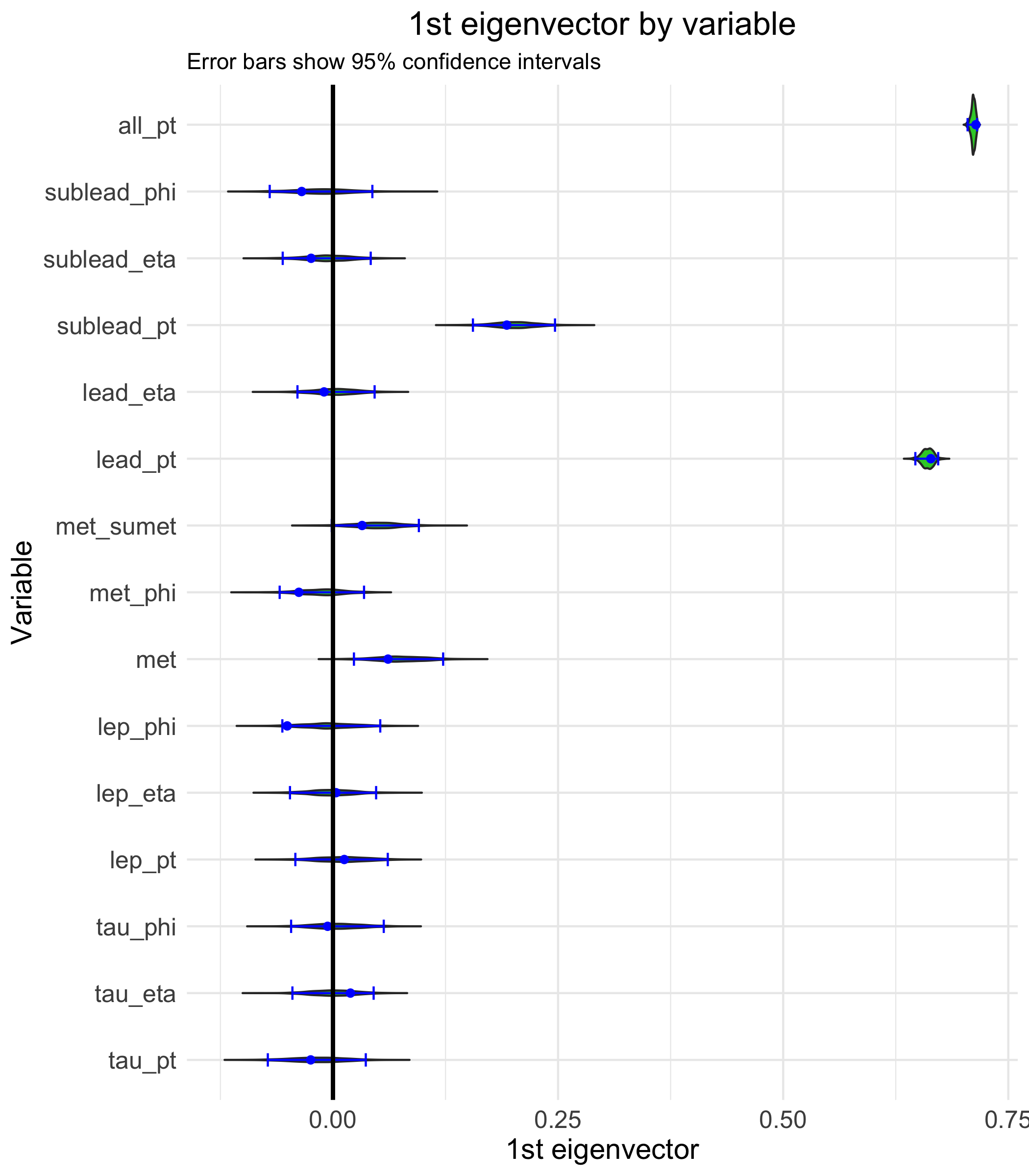
(c) First Eigenvector

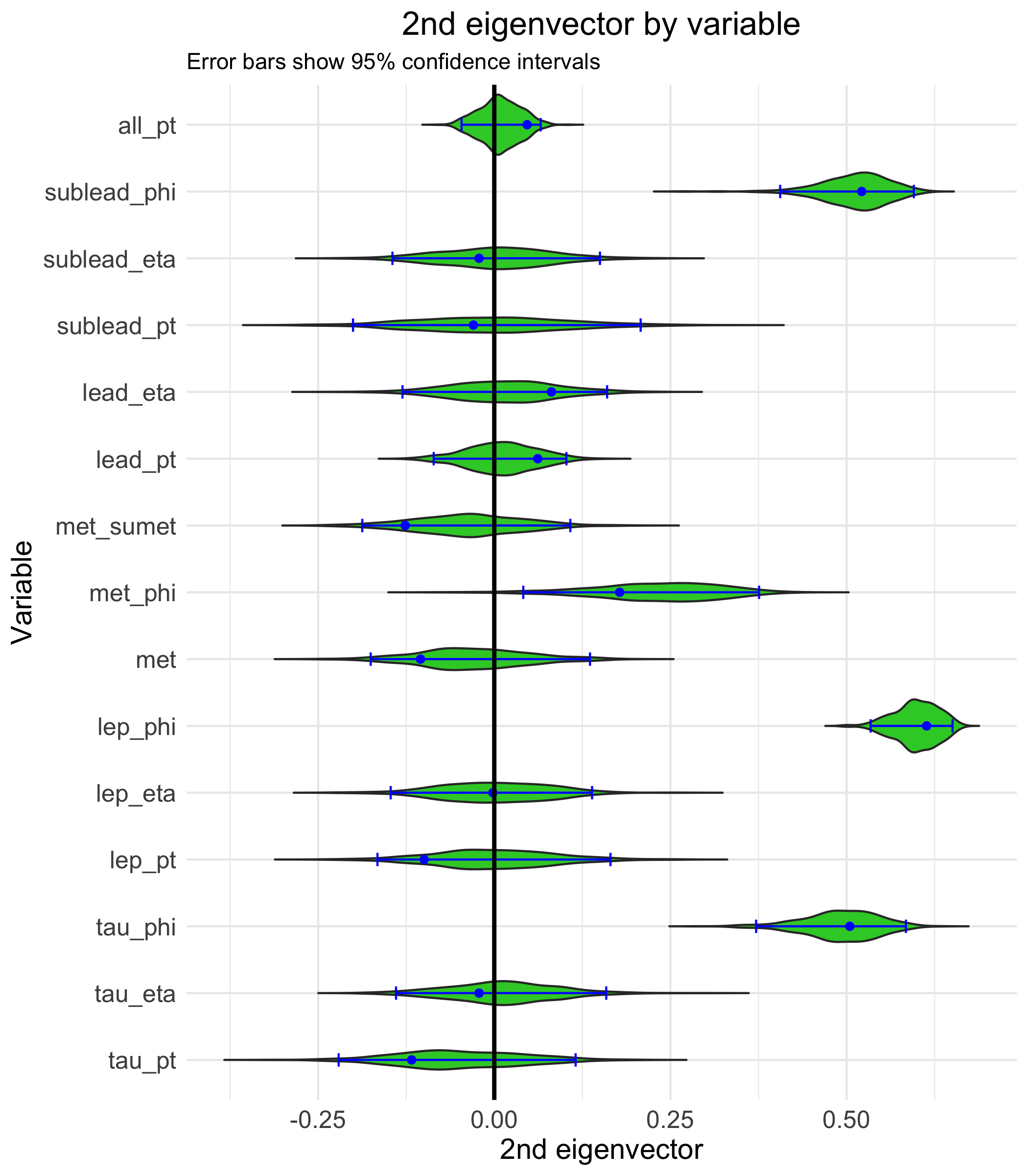
(d) Second Eigenvector

Figure 8: The active subspace variables for the classifier trained on data with signal strength $\lambda=0.15$ computed using a local linear smoother that uses the gaussian kernel with smoothing parameter $h=0.5$. (a) gives the distribution of the standardized gradients $\widehat{\beta}_{j}(Z_{i})/\widehat{sd(\widehat{\beta}_{j}(Z_{i}))}$ given by the local linear smoother at every point in the combined test data $Z_{i}\in\mathcal{X}_{2}\cup\mathcal{W}_{2}$. The dots denote the mean. In (b), (c) and (d), the violin plot and the dashes give the bootstrapped empirical distribution and the bootstrapped uncertainty intervals computed using the empirical quantiles respectively for the standardized mean, the first eigenvector and the second eigenvector. In (b) the dots give the mean standardized gradient similar to (a). In (c) and (d) the dots represent the first eigenvector and the second eigenvector computed on the combined test data, respectively.

The mean standardized gradient in Figure 8(b) gives the direction in which the classifier output changes most rapidly on average. We see that jointly higher transverse momentums of the hadronic tau (tau_pt) and the remaining lepton (lep_pt) contribute the most to an increase in the classifier output. Increase in these transverse momentums, combined with a decrease in the transverse momentum of the leading jet (lead_pt) and the scalar sum of the transverse momentum of all the jets (all_pt), leads to an increase in the classifier output. This implies that the detected signal events display higher momentums of the hadronic tau and the other lepton, lower momentums of the leading jet and lower scalar sum of the momentums of all the jets as compared to background events. Note that the mean gradient vector not only captures the dependency of the classifier on each variable individually, but also characterizes the multivariable dependencies that influence the classifier.

The first eigenvector gives the first principal component of the gradients, which demonstrates the relationship between the variables that causes the most variability in the gradients of the classifier. The first eigenvector, as seen in Figure 8(c), indicates that when all_pt, the scalar sum of the transverse momentums, lead_pt, the transverse momentum of the leading jet, sublead_pt, the transverse momentum of the subleading jet and met, the missing transverse energy, jointly change in the same direction, it causes the most variation in the classifier. This means that these variables together, help the classifier separate the signal from the background. The second eigenvector, i.e., the second principal component of the gradients, as seen in Figure 8(d), appears to capture the relationship between the azimuth angle $\phi$ of the different objects in the event that most influences the classifier. Recall that the $\phi$ values of the objects have been transformed to denote the difference in the angle between each object and the leading jet. So, the second eigenvector indicates that the $\phi$ angle between the leading jet and all the other four objects (the subleading jet, the hadronic tau, the lepton and the missing transverse energy) influences the classifier. This has an appealing physical interpretation in that it indicates that the azimuthal orientation between the leading jet and the rest of the event is a useful feature for separating the signal from the background.

Remark.

Note that for any eigenvector $M_{\cdot j}$ of the standardized gradients of the trained classifier, $-M_{\cdot j}$ is also an eigenvector. This causes the violin plots of the bootstrapped eigenvectors to be systematically symmetric about zero. To solve this problem, we first take the variable that has the largest absolute eigenvector value, i.e. $k_{j}=\arg\max_{i}|\widehat{M}_{ij}|$. Then we fix the sign of the bootstrapped eigenvectors $\widehat{M}_{\cdot j}^{*}$ such that the sign of the $k_{j}^{th}$ variable matches, i.e., $\text{sgn}(\widehat{M}_{k_{j}j}^{*})=\text{sgn}(\widehat{M}_{k_{j}j})$. This process has been followed in Figures 8(c) and 8(d) to handle the problem.

So, the active subspace methods provide an algorithm to interpret the semi-supervised classifier once it has detected a signal in the experimental data. The methods imply that the classifier that detects the Higgs boson is positively influenced by tau_pt and lep_pt, and negatively influenced by all_pt and lead_pt. Additionally, it is also influenced by joint changes in the values of all_pt, lead_pt, lsubead_pt and lmet. The classifier is also influenced by the difference between the azimuth angle $\phi$ of the leading jet and those of the other four objects, indicating that this might be an important feature for detecting the signal events. Finally, we note that without techniques like these it would have been very difficult to understand what kind of a signal the semi-supervised classifier has detected within the high-dimensional feature space.

7 Conclusion

In this paper, we studied model-independent anomaly detection tests using semi-supervised classifiers, that can detect the presence of signal events hidden within background events in high energy particle physics data sets. Additionally, we proposed methods to estimate the signal strength and to identify the active subspace affecting the classifier most strongly, leading to an understanding of the detected signal. We demonstrated the performance of the methods and also compared the proposed tests with comparable model-dependent supervised methods as well as nearest neighbor two-sample tests on a data set related to the search for the Higgs boson at the Large Hadron Collider.

We presented multiple model-independent methods that search for the signal without assuming any knowledge of the signal model. By not assuming any signal model, we retain the ability to detect unknown and unexpected signals. This is an important capability for future searches at the Large Hadron Collider, where model-dependent searches have so far not yielded evidence of physics beyond the Standard Model. We used a semi-supervised classifier to distinguish the experimental data from the background data and used the performance of the classifier to perform a test to detect a significant difference between the two data sets. We proposed three test statistics that can be used for the test: the likelihood ratio test (LRT) statistic, the area under the curve (AUC) statistic and the misclassification error (MCE) statistic.

We compared the use of the different test statistics, as well as the use of different techniques for obtaining the null distribution, in building the test that has the most power in detecting the signal. We compared the power of the methods to detect the Higgs boson at different signal strengths and showed that a version of the proposed AUC method has power that is competitive with the model-dependent methods. So, even when the signal model is correctly assumed by the model-dependent methods, the proposed model-independent methods appear to still have competitive power to detect the presence of the signal. However, when the signal model is incorrectly assumed or misspecified, the model-dependent methods can totally miss the signal, whereas the proposed model-independent ones are still able to detect the signal, as demonstrated in our experiments. In particular, the proposed methods demonstrate the ability to find new particles without specific a priori knowledge of their properties.

As described in Section 3.1, model-dependent methods currently in use in experimental high-energy physics, are slightly different from the ones presented in Section 3.1. In this paper, to make the model-dependent methods comparable to the proposed model-independent ones, we consider high-dimensional model-dependent tests. In current practice though, a threshold is placed on the supervised classifier output to select a subset of the experimental data that is richer in signal events. Then the high-dimensional data set is transformed into a univariate one, and the transformed data are fitted using a one-dimensional mixture model consisting of signal and background components. This is used to construct a profile likelihood ratio test (ATLAS Collaboration and CMS Collaboration, 2011), where some of the nuisance parameters are related to the one-dimensional background model. Dauncey et al. (2015) proposed a discrete profiling method for this test based on considering the choice of the background functional form as a discrete nuisance parameter which is profiled in an analogous way to continuous nuisance parameters.

These considerations motivate multiple avenues for future exploration. We could construct an analogous model-independent version of the approach described above, where we first use the semi-supervised classifier output to select a signal-rich subset of the experimental data, then transform the selected data to a one-dimensional space and finally perform a test in the one-dimensional space using a mixture model. For well-chosen transformations, this could increase the power of the test. More interestingly, for many signals, the signal distribution corresponding to a transformation into the invariant mass variable is predicted by quantum mechanics to be the Cauchy distribution (also known as the Breit–Wigner distribution in particle physics; see Chapter 49 in Particle Data Group (2020)), whose parameters, under the model-independent scenario, are unknown to us. It would be interesting to built this knowledge into the semi-supervised method. A straightforward approach would be to simply use the Cauchy distribution, convolved with a model for detector smearing, in the one-dimensional mixture model, but it might also be possible to incorporate this knowledge into the training of the high-dimensional semi-supervised classifier.

Another important avenue of future work would be to find ways to account for systematic uncertainties in the background training data. As described above, the current supervised techniques account for systematics using profile likelihoods for one-dimensional summary statistics, with the systematic variations in the one-dimensional space parameterized using potentially hundreds or thousands of nuisance parameters. This should also be feasible for one-dimensional semi-supervised tests. However, it might also be possible to use profiling in the high-dimensional semi-supervised likelihood ratio tests. For example, if we had two plausible background samples from two different MC generators, we could use optimal transport (Peyré et al., 2019) to find the geodesic between the samples. We could then profile over the parameter corresponding to the location on the geodesic, which would account for the systematic uncertainty corresponding to the envelope of background models spanned by the two MC generators.

[Acknowledgments] The authors would like to thank the anonymous referees, the Associate Editor and the Editor of Annals of Applied Statistics for their extensive, thoughtful and constructive comments that greatly improved the quality of this paper. This work was supported in part by NSF awards PHY-2020295, DMS-2053804 and DMS-2113684.

Supplement to “Model-Independent Detection of New Physics Signals Using Interpretable Semi-Supervised Classifier Tests” The supplementary material contains the proof of Theorem 4.1, some of the proposed algorithms from Section 3.2, and details about the exploratory data analysis of the Higgs boson data used in the experiments in Section 6. It additionally describes the selection of the smoothing parameter for the active subspace methods. The supplementary material can be found at https://github.com/purvashac/MIDetectionClassifierTests/blob/main/Supplementary.pdf

References

- Adam-Bourdarios et al. (2015) {binproceedings}[author] \bauthor\bsnmAdam-Bourdarios, \bfnmClaire\binitsC., \bauthor\bsnmCowan, \bfnmGlen\binitsG., \bauthor\bsnmGermain, \bfnmCécile\binitsC., \bauthor\bsnmGuyon, \bfnmIsabelle\binitsI., \bauthor\bsnmKégl, \bfnmBalàzs\binitsB. and \bauthor\bsnmRousseau, \bfnmDavid\binitsD. (\byear2015). \btitleThe Higgs boson machine learning challenge. In \bbooktitleProceedings of the NIPS 2014 Workshop on High-energy Physics and Machine Learning (\beditor\bfnmGlen\binitsG. \bsnmCowan, \beditor\bfnmCécile\binitsC. \bsnmGermain, \beditor\bfnmIsabelle\binitsI. \bsnmGuyon, \beditor\bfnmBalàzs\binitsB. \bsnmKégl and \beditor\bfnmDavid\binitsD. \bsnmRousseau, eds.). \bseriesProceedings of Machine Learning Research \bvolume42 \bpages19–55. \bpublisherPMLR, \baddressMontreal, Canada. \endbibitem
- Andreassen, Nachman and Shih (2020) {barticle}[author] \bauthor\bsnmAndreassen, \bfnmAnders\binitsA., \bauthor\bsnmNachman, \bfnmBenjamin\binitsB. and \bauthor\bsnmShih, \bfnmDavid\binitsD. (\byear2020). \btitleSimulation assisted likelihood-free anomaly detection. \bjournalPhysical Review D \bvolume101 \bpages095004. \bdoi10.1103/PhysRevD.101.095004 \endbibitem
- Bach et al. (2015) {barticle}[author] \bauthor\bsnmBach, \bfnmSebastian\binitsS., \bauthor\bsnmBinder, \bfnmAlexander\binitsA., \bauthor\bsnmMontavon, \bfnmGrégoire\binitsG., \bauthor\bsnmKlauschen, \bfnmFrederick\binitsF., \bauthor\bsnmMüller, \bfnmKlaus-Robert\binitsK.-R. and \bauthor\bsnmSamek, \bfnmWojciech\binitsW. (\byear2015). \btitleOn pixel-wise explanations for non-linear classifier decisions by layer-wise relevance propagation. \bjournalPloS One \bvolume10 \bpagese0130140. \bdoihttps://doi.org/10.1371/journal.pone.0130140 \endbibitem
- Behnke et al. (2013) {bbook}[author] \bauthor\bsnmBehnke, \bfnmOlaf\binitsO., \bauthor\bsnmKröninger, \bfnmKevin\binitsK., \bauthor\bsnmSchott, \bfnmGrégory\binitsG. and \bauthor\bsnmSchörner-Sadenius, \bfnmThomas\binitsT. (\byear2013). \btitleData Analysis in High Energy Physics: A Practical Guide to Statistical Methods. \bpublisherJohn Wiley & Sons. \endbibitem
- Bhat (2011) {barticle}[author] \bauthor\bsnmBhat, \bfnmPushpalatha C\binitsP. C. (\byear2011). \btitleMultivariate analysis methods in particle physics. \bjournalAnnual Review of Nuclear and Particle Science \bvolume61 \bpages281–309. \endbibitem
- Böhning et al. (1994) {barticle}[author] \bauthor\bsnmBöhning, \bfnmDankmar\binitsD., \bauthor\bsnmDietz, \bfnmEkkehart\binitsE., \bauthor\bsnmSchaub, \bfnmRainer\binitsR., \bauthor\bsnmSchlattmann, \bfnmPeter\binitsP. and \bauthor\bsnmLindsay, \bfnmBruce G\binitsB. G. (\byear1994). \btitleThe distribution of the likelihood ratio for mixtures of densities from the one-parameter exponential family. \bjournalAnnals of the Institute of Statistical Mathematics \bvolume46 \bpages373–388. \endbibitem
- Boström (2008) {binproceedings}[author] \bauthor\bsnmBoström, \bfnmHenrik\binitsH. (\byear2008). \btitleCalibrating random forests. In \bbooktitle2008 Seventh International Conference on Machine Learning and Applications \bpages121-126. \bdoi10.1109/ICMLA.2008.107 \endbibitem
- Breiman (2001) {barticle}[author] \bauthor\bsnmBreiman, \bfnmLeo\binitsL. (\byear2001). \btitleRandom forests. \bjournalMachine Learning \bvolume45 \bpages5–32. \endbibitem
- Casa and Menardi (2018) {barticle}[author] \bauthor\bsnmCasa, \bfnmAlessandro\binitsA. and \bauthor\bsnmMenardi, \bfnmGiovanna\binitsG. (\byear2018). \btitleNonparametric semisupervised classification for signal detection in high energy physics. \bjournalarXiv preprint arXiv:1809.02977. \endbibitem
- Chakravarti et al. (2022) {barticle}[author] \bauthor\bsnmChakravarti, \bfnmPurvasha\binitsP., \bauthor\bsnmKuusela, \bfnmMikael\binitsM., \bauthor\bsnmLei, \bfnmJing\binitsJ. and \bauthor\bsnmWasserman, \bfnmLarry\binitsL. (\byear2022). \btitleSupplement to “Model-Independent Detection of Signals Using Interpretable Semi-Supervised Classifier Tests.”. \endbibitem
- Chandola, Banerjee and Kumar (2009) {barticle}[author] \bauthor\bsnmChandola, \bfnmVarun\binitsV., \bauthor\bsnmBanerjee, \bfnmArindam\binitsA. and \bauthor\bsnmKumar, \bfnmVipin\binitsV. (\byear2009). \btitleAnomaly detection: A survey. \bjournalACM Computing Surveys (CSUR) \bvolume41 \bpages1–58. \endbibitem
- Choudalakis (2008) {barticle}[author] \bauthor\bsnmChoudalakis, \bfnmGeorgios\binitsG. (\byear2008). \btitleModel independent search for new physics at the Tevatron. \bjournalarXiv preprint arXiv:0805.3954. \endbibitem
- H1 Collaboration (2004) {barticle}[author] \bauthor\bsnmH1 Collaboration (\byear2004). \btitleA general search for new phenomena in ep scattering at HERA. \bjournalPhysics Letters B \bvolume602 \bpages14–30. \endbibitem
- CDF Collaboration (2008) {barticle}[author] \bauthor\bsnmCDF Collaboration (\byear2008). \btitleModel-independent and quasi-model-independent search for new physics at CDF. \bjournalPhysical Review D \bvolume78 \bpages012002. \bdoi10.1103/PhysRevD.78.012002 \endbibitem
- CDF Collaboration (2009) {barticle}[author] \bauthor\bsnmCDF Collaboration (\byear2009). \btitleGlobal search for new physics with at CDF. \bjournalPhysical Review D \bvolume79 \bpages011101. \endbibitem
- ATLAS Collaboration (2012a) {barticle}[author] \bauthor\bsnmATLAS Collaboration (\byear2012a). \btitleObservation of a new particle in the search for the Standard Model Higgs boson with the ATLAS detector at the LHC. \bjournalPhysics Letters B \bvolume716 \bpages1–29. \endbibitem
- CMS Collaboration (2012b) {barticle}[author] \bauthor\bsnmCMS Collaboration (\byear2012b). \btitleObservation of a new boson at a mass of 125 GeV with the CMS experiment at the LHC. \bjournalPhysics Letters B \bvolume716 \bpages30–61. \endbibitem
- D0 Collaboration (2012c) {barticle}[author] \bauthor\bsnmD0 Collaboration (\byear2012c). \btitleModel independent search for new phenomena in pp (bar) collisions at TeV. \bjournalPhysical Review D \bvolume85. \endbibitem
- ATLAS Collaboration (2014) {barticle}[author] \bauthor\bsnmATLAS Collaboration (\byear2014). \btitleDataset from the ATLAS Higgs Boson Machine Learning Challenge 2014. \bjournalCERN Open Data Portal. \bdoi10.7483/OPENDATA.ATLAS.ZBP2.M5T8 \endbibitem
- CMS Collaboration (2017) {barticle}[author] \bauthor\bsnmCMS Collaboration (\byear2017). \btitleMUSiC, a model unspecific search for new physics, in pp collisions at TeV. \bjournalCMS Physics Analysis Summary CMS-PAS-EXO-14/016. \endbibitem
- ATLAS Collaboration (2019) {barticle}[author] \bauthor\bsnmATLAS Collaboration (\byear2019). \btitleA strategy for a general search for new phenomena using data-derived signal regions and its application within the ATLAS experiment. \bjournalThe European Physical Journal C \bvolume79 \bpages120. \endbibitem
- CMS Collaboration (2020) {btechreport}[author] \bauthor\bsnmCMS Collaboration (\byear2020). \btitleMUSiC, a model unspecific search for new physics, in pp collisions at sqrt (s)= 13 TeV \btypeTechnical Report, \bpublisherTechnical report CMS-PAS-EXO-19-008, CERN, Geneva. \endbibitem
- ATLAS Collaboration and CMS Collaboration (2011) {btechreport}[author] \bauthor\bsnmATLAS Collaboration and CMS Collaboration (\byear2011). \btitleLHC Higgs Combination Group, Procedure for the LHC Higgs boson search combination in Summer 2011 \btypeTechnical Report, \bpublisherCMS-NOTE-2011-005. \endbibitem
- Collins, Howe and Nachman (2018) {barticle}[author] \bauthor\bsnmCollins, \bfnmJack\binitsJ., \bauthor\bsnmHowe, \bfnmKiel\binitsK. and \bauthor\bsnmNachman, \bfnmBenjamin\binitsB. (\byear2018). \btitleAnomaly detection for resonant new physics with machine learning. \bjournalPhysical Review Letters \bvolume121 \bpages241803. \endbibitem
- Collins, Howe and Nachman (2019) {barticle}[author] \bauthor\bsnmCollins, \bfnmJack H\binitsJ. H., \bauthor\bsnmHowe, \bfnmKiel\binitsK. and \bauthor\bsnmNachman, \bfnmBenjamin\binitsB. (\byear2019). \btitleExtending the search for new resonances with machine learning. \bjournalPhysical Review D \bvolume99 \bpages014038. \endbibitem
- Constantine (2015) {bbook}[author] \bauthor\bsnmConstantine, \bfnmPaul G\binitsP. G. (\byear2015). \btitleActive subspaces: Emerging ideas for dimension reduction in parameter studies \bvolume2. \bpublisherSIAM. \endbibitem
- Constantine, Dow and Wang (2014) {barticle}[author] \bauthor\bsnmConstantine, \bfnmPaul G\binitsP. G., \bauthor\bsnmDow, \bfnmEric\binitsE. and \bauthor\bsnmWang, \bfnmQiqi\binitsQ. (\byear2014). \btitleActive subspace methods in theory and practice: applications to kriging surfaces. \bjournalSIAM Journal on Scientific Computing \bvolume36 \bpagesA1500–A1524. \endbibitem
- Constantine et al. (2015) {barticle}[author] \bauthor\bsnmConstantine, \bfnmPaul G\binitsP. G., \bauthor\bsnmEmory, \bfnmMichael\binitsM., \bauthor\bsnmLarsson, \bfnmJohan\binitsJ. and \bauthor\bsnmIaccarino, \bfnmGianluca\binitsG. (\byear2015). \btitleExploiting active subspaces to quantify uncertainty in the numerical simulation of the HyShot II scramjet. \bjournalJournal of Computational Physics \bvolume302 \bpages1–20. \endbibitem
- Cowan et al. (2011) {barticle}[author] \bauthor\bsnmCowan, \bfnmGlen\binitsG., \bauthor\bsnmCranmer, \bfnmKyle\binitsK., \bauthor\bsnmGross, \bfnmEilam\binitsE. and \bauthor\bsnmVitells, \bfnmOfer\binitsO. (\byear2011). \btitleAsymptotic formulae for likelihood-based tests of new physics. \bjournalThe European Physical Journal C \bvolume71 \bpages1554. \endbibitem
- Cranmer (2015) {barticle}[author] \bauthor\bsnmCranmer, \bfnmKyle\binitsK. (\byear2015). \btitlePractical statistics for the LHC. \bjournalarXiv preprint arXiv:1503.07622. \endbibitem
- Cranmer, Pavez and Louppe (2015) {barticle}[author] \bauthor\bsnmCranmer, \bfnmKyle\binitsK., \bauthor\bsnmPavez, \bfnmJuan\binitsJ. and \bauthor\bsnmLouppe, \bfnmGilles\binitsG. (\byear2015). \btitleApproximating likelihood ratios with calibrated discriminative classifiers. \bjournalarXiv preprint arXiv:1506.02169. \endbibitem
- Cui et al. (2020) {barticle}[author] \bauthor\bsnmCui, \bfnmChunfeng\binitsC., \bauthor\bsnmZhang, \bfnmKaiqi\binitsK., \bauthor\bsnmDaulbaev, \bfnmTalgat\binitsT., \bauthor\bsnmGusak, \bfnmJulia\binitsJ., \bauthor\bsnmOseledets, \bfnmIvan\binitsI. and \bauthor\bsnmZhang, \bfnmZheng\binitsZ. (\byear2020). \btitleActive Subspace of Neural Networks: Structural Analysis and Universal Attacks. \bjournalSIAM Journal on Mathematics of Data Science \bvolume2 \bpages1096–1122. \endbibitem
- D’Agnolo and Wulzer (2019) {barticle}[author] \bauthor\bsnmD’Agnolo, \bfnmRaffaele Tito\binitsR. T. and \bauthor\bsnmWulzer, \bfnmAndrea\binitsA. (\byear2019). \btitleLearning new physics from a machine. \bjournalPhysical Review D \bvolume99 \bpages015014. \endbibitem
- D’Agnolo et al. (2021) {barticle}[author] \bauthor\bsnmD’Agnolo, \bfnmRaffaele Tito\binitsR. T., \bauthor\bsnmGrosso, \bfnmGaia\binitsG., \bauthor\bsnmPierini, \bfnmMaurizio\binitsM., \bauthor\bsnmWulzer, \bfnmAndrea\binitsA. and \bauthor\bsnmZanetti, \bfnmMarco\binitsM. (\byear2021). \btitleLearning multivariate new physics. \bjournalThe European Physical Journal C \bvolume81 \bpages1–21. \endbibitem
- D’Agnolo et al. (2022) {barticle}[author] \bauthor\bsnmD’Agnolo, \bfnmRaffaele Tito\binitsR. T., \bauthor\bsnmGrosso, \bfnmGaia\binitsG., \bauthor\bsnmPierini, \bfnmMaurizio\binitsM., \bauthor\bsnmWulzer, \bfnmAndrea\binitsA. and \bauthor\bsnmZanetti, \bfnmMarco\binitsM. (\byear2022). \btitleLearning new physics from an imperfect machine. \bjournalThe European Physical Journal C \bvolume82 \bpages1–37. \endbibitem
- Dauncey et al. (2015) {barticle}[author] \bauthor\bsnmDauncey, \bfnmPD\binitsP., \bauthor\bsnmKenzie, \bfnmM\binitsM., \bauthor\bsnmWardle, \bfnmN\binitsN. and \bauthor\bsnmDavies, \bfnmGJ\binitsG. (\byear2015). \btitleHandling uncertainties in background shapes: the discrete profiling method. \bjournalJournal of Instrumentation \bvolume10 \bpagesP04015. \endbibitem
- Davison and Hinkley (1997) {bbook}[author] \bauthor\bsnmDavison, \bfnmAnthony Christopher\binitsA. C. and \bauthor\bsnmHinkley, \bfnmDavid Victor\binitsD. V. (\byear1997). \btitleBootstrap Methods and their Application \bvolume1. \bpublisherCambridge University Press. \endbibitem
- Dobson and Barnett (2018) {bbook}[author] \bauthor\bsnmDobson, \bfnmAnnette J\binitsA. J. and \bauthor\bsnmBarnett, \bfnmAdrian G\binitsA. G. (\byear2018). \btitleAn Introduction to Generalized Linear Models. \bpublisherCRC press. \endbibitem
- Dorigo and de Castro (2020) {barticle}[author] \bauthor\bsnmDorigo, \bfnmTommaso\binitsT. and \bauthor\bparticlede \bsnmCastro, \bfnmPablo\binitsP. (\byear2020). \btitleDealing with nuisance parameters using machine learning in high energy physics: A review. \bjournalarXiv preprint arXiv:2007.09121. \endbibitem
- Efron and Tibshirani (1994) {bbook}[author] \bauthor\bsnmEfron, \bfnmBradley\binitsB. and \bauthor\bsnmTibshirani, \bfnmRobert J\binitsR. J. (\byear1994). \btitleAn Introduction to the Bootstrap. \bpublisherCRC press. \endbibitem
- Friedman (2003) {binproceedings}[author] \bauthor\bsnmFriedman, \bfnmJerome H.\binitsJ. H. (\byear2003). \btitleOn multivariate goodness-of-fit and two-sample testing. In \bbooktitlePHYSTAT 2003, SLAC, Stanford, California. \endbibitem
- Ghosh, Nachman and Whiteson (2021) {barticle}[author] \bauthor\bsnmGhosh, \bfnmAishik\binitsA., \bauthor\bsnmNachman, \bfnmBenjamin\binitsB. and \bauthor\bsnmWhiteson, \bfnmDaniel\binitsD. (\byear2021). \btitleUncertainty-aware machine learning for high energy physics. \bjournalPhysical Review D \bvolume104 \bpages056026. \bdoi10.1103/PhysRevD.104.056026 \endbibitem
- Ghosh and Sen (1984) {barticle}[author] \bauthor\bsnmGhosh, \bfnmJayanta K\binitsJ. K. and \bauthor\bsnmSen, \bfnmPranab Kumar\binitsP. K. (\byear1984). \btitleOn the asymptotic performance of the log likelihood ratio statistic for the mixture model and related results. \bjournalBerkeley Conference In Honor of Jerzy Neyman and Jack Kiefer. \endbibitem
- Goodfellow et al. (2014) {binproceedings}[author] \bauthor\bsnmGoodfellow, \bfnmIan\binitsI., \bauthor\bsnmPouget-Abadie, \bfnmJean\binitsJ., \bauthor\bsnmMirza, \bfnmMehdi\binitsM., \bauthor\bsnmXu, \bfnmBing\binitsB., \bauthor\bsnmWarde-Farley, \bfnmDavid\binitsD., \bauthor\bsnmOzair, \bfnmSherjil\binitsS., \bauthor\bsnmCourville, \bfnmAaron\binitsA. and \bauthor\bsnmBengio, \bfnmYoshua\binitsY. (\byear2014). \btitleGenerative adversarial nets. In \bbooktitleAdvances in neural information processing systems \bpages2672–2680. \endbibitem
- Grömping (2009) {barticle}[author] \bauthor\bsnmGrömping, \bfnmUlrike\binitsU. (\byear2009). \btitleVariable importance assessment in regression: linear regression versus random forest. \bjournalThe American Statistician \bvolume63 \bpages308–319. \endbibitem
- Particle Data Group (2020) {barticle}[author] \bauthor\bsnmParticle Data Group (\byear2020). \btitleReview of Particle Physics. \bjournalPTEP \bvolume2020 \bpages083C01. \bdoi10.1093/ptep/ptaa104 \endbibitem
- Hanley et al. (1989) {barticle}[author] \bauthor\bsnmHanley, \bfnmJohn A\binitsJ. A. \betalet al. (\byear1989). \btitleReceiver operating characteristic (ROC) methodology: the state of the art. \bjournalCrit Rev Diagn Imaging \bvolume29 \bpages307–335. \endbibitem
- Hanley and McNeil (1982) {barticle}[author] \bauthor\bsnmHanley, \bfnmJames A\binitsJ. A. and \bauthor\bsnmMcNeil, \bfnmBarbara J\binitsB. J. (\byear1982). \btitleThe meaning and use of the area under a receiver operating characteristic (ROC) curve. \bjournalRadiology \bvolume143 \bpages29–36. \endbibitem
- Hastie, Tibshirani and Friedman (2009) {bbook}[author] \bauthor\bsnmHastie, \bfnmTrevor\binitsT., \bauthor\bsnmTibshirani, \bfnmRobert\binitsR. and \bauthor\bsnmFriedman, \bfnmJerome H\binitsJ. H. (\byear2009). \btitleThe Elements of Statistical Learning: Data Mining, Inference, and Prediction \bvolume2. \bpublisherSpringer. \endbibitem
- Henze (1988) {barticle}[author] \bauthor\bsnmHenze, \bfnmNorbert\binitsN. (\byear1988). \btitleA multivariate two-sample test based on the number of nearest neighbor type coincidences. \bjournalThe Annals of Statistics \bpages772–783. \endbibitem
- Ishwaran et al. (2007) {barticle}[author] \bauthor\bsnmIshwaran, \bfnmHemant\binitsH. \betalet al. (\byear2007). \btitleVariable importance in binary regression trees and forests. \bjournalElectronic Journal of Statistics \bvolume1 \bpages519–537. \endbibitem
- Kasieczka et al. (2021) {barticle}[author] \bauthor\bsnmKasieczka, \bfnmGregor\binitsG., \bauthor\bsnmNachman, \bfnmBenjamin\binitsB., \bauthor\bsnmShih, \bfnmDavid\binitsD., \bauthor\bsnmAmram, \bfnmOz\binitsO., \bauthor\bsnmAndreassen, \bfnmAnders\binitsA., \bauthor\bsnmBenkendorfer, \bfnmKees\binitsK., \bauthor\bsnmBortolato, \bfnmBlaz\binitsB., \bauthor\bsnmBrooijmans, \bfnmGustaaf\binitsG., \bauthor\bsnmCanelli, \bfnmFlorencia\binitsF., \bauthor\bsnmCollins, \bfnmJack H\binitsJ. H. \betalet al. (\byear2021). \btitleThe LHC Olympics 2020: A community challenge for anomaly detection in high energy physics. \bjournalarXiv preprint arXiv:2101.08320. \endbibitem
- Kim et al. (2016) {barticle}[author] \bauthor\bsnmKim, \bfnmIlmun\binitsI., \bauthor\bsnmRamdas, \bfnmAaditya\binitsA., \bauthor\bsnmSingh, \bfnmAarti\binitsA. and \bauthor\bsnmWasserman, \bfnmLarry\binitsL. (\byear2016). \btitleClassification accuracy as a proxy for two sample testing. \bjournalarXiv preprint arXiv:1602.02210. \endbibitem
- Kim et al. (2019) {barticle}[author] \bauthor\bsnmKim, \bfnmIlmun\binitsI., \bauthor\bsnmLee, \bfnmAnn B\binitsA. B., \bauthor\bsnmLei, \bfnmJing\binitsJ. \betalet al. (\byear2019). \btitleGlobal and local two-sample tests via regression. \bjournalElectronic Journal of Statistics \bvolume13 \bpages5253–5305. \endbibitem
- Knuteson (2000) {barticle}[author] \bauthor\bsnmKnuteson, \bfnmBruce\binitsB. (\byear2000). \btitlePh.D. thesis, University of California at Berkeley. \endbibitem
- Kuusela et al. (2012) {binproceedings}[author] \bauthor\bsnmKuusela, \bfnmMikael\binitsM., \bauthor\bsnmVatanen, \bfnmTommi\binitsT., \bauthor\bsnmMalmi, \bfnmEric\binitsE., \bauthor\bsnmRaiko, \bfnmTapani\binitsT., \bauthor\bsnmAaltonen, \bfnmTimo\binitsT. and \bauthor\bsnmNagai, \bfnmYoshikazu\binitsY. (\byear2012). \btitleSemi-supervised anomaly detection–towards model-independent searches of new physics. In \bbooktitleJournal of Physics: Conference Series \bvolume368 \bpages012032. \bpublisherIOP Publishing. \endbibitem
- Lei et al. (2018) {barticle}[author] \bauthor\bsnmLei, \bfnmJing\binitsJ., \bauthor\bsnmG’Sell, \bfnmMax\binitsM., \bauthor\bsnmRinaldo, \bfnmAlessandro\binitsA., \bauthor\bsnmTibshirani, \bfnmRyan J\binitsR. J. and \bauthor\bsnmWasserman, \bfnmLarry\binitsL. (\byear2018). \btitleDistribution-free predictive inference for regression. \bjournalJournal of the American Statistical Association \bvolume113 \bpages1094–1111. \endbibitem
- Lyons and Wardle (2018) {barticle}[author] \bauthor\bsnmLyons, \bfnmLouis\binitsL. and \bauthor\bsnmWardle, \bfnmNicholas\binitsN. (\byear2018). \btitleStatistical issues in searches for new phenomena in High Energy Physics. \bjournalJournal of Physics G: Nuclear and Particle Physics \bvolume45 \bpages033001. \bdoi10.1088/1361-6471/aa9408 \endbibitem
- Metz (1978) {binproceedings}[author] \bauthor\bsnmMetz, \bfnmCharles E\binitsC. E. (\byear1978). \btitleBasic principles of ROC analysis. In \bbooktitleSeminars in nuclear medicine \bvolume8 \bpages283–298. \bpublisherElsevier. \endbibitem
- Nachman (2020) {barticle}[author] \bauthor\bsnmNachman, \bfnmBenjamin\binitsB. (\byear2020). \btitleA guide for deploying Deep Learning in LHC searches: How to achieve optimality and account for uncertainty. \bjournalSciPost Phys. \bvolume8 \bpages90. \bdoi10.21468/SciPostPhys.8.6.090 \endbibitem
- Nachman and Shih (2020) {barticle}[author] \bauthor\bsnmNachman, \bfnmBenjamin\binitsB. and \bauthor\bsnmShih, \bfnmDavid\binitsD. (\byear2020). \btitleAnomaly detection with density estimation. \bjournalPhysical Review D \bvolume101 \bpages075042. \endbibitem
- Nelder and Wedderburn (1972) {barticle}[author] \bauthor\bsnmNelder, \bfnmJohn Ashworth\binitsJ. A. and \bauthor\bsnmWedderburn, \bfnmRobert WM\binitsR. W. (\byear1972). \btitleGeneralized linear models. \bjournalJournal of the Royal Statistical Society: Series A (General) \bvolume135 \bpages370–384. \endbibitem
- Newcombe (2006) {barticle}[author] \bauthor\bsnmNewcombe, \bfnmRobert G\binitsR. G. (\byear2006). \btitleConfidence intervals for an effect size measure based on the Mann–Whitney statistic. Part 2: asymptotic methods and evaluation. \bjournalStatistics in Medicine \bvolume25 \bpages559–573. \endbibitem
- Niculescu-Mizil and Caruana (2005) {binproceedings}[author] \bauthor\bsnmNiculescu-Mizil, \bfnmAlexandru\binitsA. and \bauthor\bsnmCaruana, \bfnmRich\binitsR. (\byear2005). \btitlePredicting good probabilities with supervised learning. In \bbooktitleProceedings of the 22nd International Conference on Machine Learning. \bseriesICML 2005 \bpages625–632. \bpublisherAssociation for Computing Machinery, \baddressNew York, NY, USA. \bdoi10.1145/1102351.1102430 \endbibitem
- Peyré et al. (2019) {barticle}[author] \bauthor\bsnmPeyré, \bfnmGabriel\binitsG., \bauthor\bsnmCuturi, \bfnmMarco\binitsM. \betalet al. (\byear2019). \btitleComputational optimal transport: With applications to data science. \bjournalFoundations and Trends® in Machine Learning \bvolume11 \bpages355–607. \endbibitem
- Radovic et al. (2018) {barticle}[author] \bauthor\bsnmRadovic, \bfnmAlexander\binitsA., \bauthor\bsnmWilliams, \bfnmMike\binitsM., \bauthor\bsnmRousseau, \bfnmDavid\binitsD., \bauthor\bsnmKagan, \bfnmMichael\binitsM., \bauthor\bsnmBonacorsi, \bfnmDaniele\binitsD., \bauthor\bsnmHimmel, \bfnmAlexander\binitsA., \bauthor\bsnmAurisano, \bfnmAdam\binitsA., \bauthor\bsnmTerao, \bfnmKazuhiro\binitsK. and \bauthor\bsnmWongjirad, \bfnmTaritree\binitsT. (\byear2018). \btitleMachine learning at the energy and intensity frontiers of particle physics. \bjournalNature \bvolume560 \bpages41–48. \endbibitem
- Reiss (2012) {bbook}[author] \bauthor\bsnmReiss, \bfnmR-D\binitsR.-D. (\byear2012). \btitleA Course on Point Processes. \bpublisherSpringer Science & Business Media. \endbibitem
- Schilling (1986) {barticle}[author] \bauthor\bsnmSchilling, \bfnmMark F\binitsM. F. (\byear1986). \btitleMultivariate two-sample tests based on nearest neighbors. \bjournalJournal of the American Statistical Association \bvolume81 \bpages799–806. \endbibitem
- Shrikumar, Greenside and Kundaje (2017) {barticle}[author] \bauthor\bsnmShrikumar, \bfnmAvanti\binitsA., \bauthor\bsnmGreenside, \bfnmPeyton\binitsP. and \bauthor\bsnmKundaje, \bfnmAnshul\binitsA. (\byear2017). \btitleLearning important features through propagating activation differences. \bjournalarXiv preprint arXiv:1704.02685. \endbibitem
- Soha (2008) {binproceedings}[author] \bauthor\bsnmSoha, \bfnmAron L.\binitsA. L. (\byear2008). \btitleGeneral searches for new physics. In \bbooktitle34th International Conference on High Energy Physics. \endbibitem
- Storey (2002) {barticle}[author] \bauthor\bsnmStorey, \bfnmJohn D\binitsJ. D. (\byear2002). \btitleA direct approach to false discovery rates. \bjournalJournal of the Royal Statistical Society: Series B (Statistical Methodology) \bvolume64 \bpages479–498. \endbibitem
- Strobl et al. (2008) {barticle}[author] \bauthor\bsnmStrobl, \bfnmCarolin\binitsC., \bauthor\bsnmBoulesteix, \bfnmAnne-Laure\binitsA.-L., \bauthor\bsnmKneib, \bfnmThomas\binitsT., \bauthor\bsnmAugustin, \bfnmThomas\binitsT. and \bauthor\bsnmZeileis, \bfnmAchim\binitsA. (\byear2008). \btitleConditional variable importance for random forests. \bjournalBMC bioinformatics \bvolume9 \bpages307. \endbibitem
- Sundararajan, Taly and Yan (2017) {barticle}[author] \bauthor\bsnmSundararajan, \bfnmMukund\binitsM., \bauthor\bsnmTaly, \bfnmAnkur\binitsA. and \bauthor\bsnmYan, \bfnmQiqi\binitsQ. (\byear2017). \btitleAxiomatic attribution for deep networks. \bjournalarXiv preprint arXiv:1703.01365. \endbibitem
- Van der Laan (2006) {barticle}[author] \bauthor\bparticleVan der \bsnmLaan, \bfnmMark J\binitsM. J. (\byear2006). \btitleStatistical inference for variable importance. \bjournalThe International Journal of Biostatistics \bvolume2. \endbibitem
- Vatanen et al. (2012) {binproceedings}[author] \bauthor\bsnmVatanen, \bfnmTommi\binitsT., \bauthor\bsnmKuusela, \bfnmMikael\binitsM., \bauthor\bsnmMalmi, \bfnmEric\binitsE., \bauthor\bsnmRaiko, \bfnmTapani\binitsT., \bauthor\bsnmAaltonen, \bfnmTimo\binitsT. and \bauthor\bsnmNagai, \bfnmYoshikazu\binitsY. (\byear2012). \btitleSemi-supervised detection of collective anomalies with an application in high energy particle physics. In \bbooktitleThe 2012 International Joint Conference on Neural Networks (IJCNN) \bpages1–8. \bpublisherIEEE. \endbibitem
- Williamson et al. (2020) {barticle}[author] \bauthor\bsnmWilliamson, \bfnmBrian D\binitsB. D., \bauthor\bsnmGilbert, \bfnmPeter B\binitsP. B., \bauthor\bsnmSimon, \bfnmNoah R\binitsN. R. and \bauthor\bsnmCarone, \bfnmMarco\binitsM. (\byear2020). \btitleA unified approach for inference on algorithm-agnostic variable importance. \bjournalarXiv preprint arXiv:2004.03683. \endbibitem