Simulation-based Optimization and Sensibility Analysis of MPI Applications: Variability Matters

Abstract

Finely tuning MPI applications and understanding the influence of key parameters (number of processes, granularity, collective operation algorithms, virtual topology, and process placement) is critical to obtain good performance on supercomputers. With the high consumption of running applications at scale, doing so solely to optimize their performance is particularly costly. Having inexpensive but faithful predictions of expected performance could be a great help for researchers and system administrators. The methodology we propose decouples the complexity of the platform, which is captured through statistical models of the performance of its main components (MPI communications, BLAS operations), from the complexity of adaptive applications by emulating the application and skipping regular non-MPI parts of the code. We demonstrate the capability of our method with High-Performance Linpack (HPL), the benchmark used to rank supercomputers in the TOP500, which requires careful tuning. We briefly present (1) how the open-source version of HPL can be slightly modified to allow a fast emulation on a single commodity server at the scale of a supercomputer. Then we present (2) an extensive (in)validation study that compares simulation with real experiments and demonstrates our ability to predict the performance of HPL within a few percent consistently. This study allows us to identify the main modeling pitfalls (e.g., spatial and temporal node variability or network heterogeneity and irregular behavior) that need to be considered. Last, we show (3) how our “surrogate” allows studying several subtle HPL parameter optimization problems while accounting for uncertainty on the platform.

Keywords: Simulation, validation, sensibility analysis, SimGrid, HPL

1 Introduction

Today, supercomputers with 100,000 cores and more are common, and several machines beyond the 1,000,000 cores mark are already in production. These compute resources are interconnected through complex non-uniform memory hierarchies and network infrastructures. This complexity requires careful optimization of application parameters, such as granularity, process organization, or algorithm choice, as these have an enormous impact on load distribution and network usage. Scientific application developers and users often spend a substantial amount of time and effort running their applications at different scales solely to tune parameters for optimizing their performance. Whenever actual performance does not match expectations, it can be challenging to understand whether the mismatch originates from application misunderstanding or machine misconfiguration. Similar difficulties are encountered when (co-)designing supercomputers for specific applications. A large part of this tuning work could be simplified if a generic and faithful performance prediction tool was available. This article presents a decisive step in this direction.

Several techniques have been proposed to predict the performance of a given application on a supercomputer. A first approach consists in building a mathematical performance model (i.e., an analytic formula) accounting for both platform and application key characteristics. However, it is rarely accurate, except for elementary applications on highly regular and well-provisioned platforms, and can thus be merely used to predict broad trends. A more precise approach consists in capturing a trace of the application at scale and replaying it using a simulator. This is an effective approach for capacity planning, but since the application trace is specific to a given set of parameters (and even specific to a given run for dynamic applications that exhibit non-deterministic behaviors due to, e.g., the use of asynchronous collective operations), it cannot be used to study how application parameters should be set for optimizing performance. The main difficulty resides in capturing and modeling the interplay between the application and the platform while faithfully accounting for their respective complexity. A promising approach recently pioneered in several tools[1, 2, 3] consists in emulating the application in a controlled way so that a platform simulator governs its execution. Although this approach’s scalability is a primary concern that has already received lots of attention, the accuracy of the simulation is even more challenging. It is still an open research question since Engelmann and Naughton[4] report, for example, an error ranging from 20% to 40% for NPB LU when using 128 ranks.

In a previous publication[5], we presented how an application like HPL can be emulated at a reasonable cost on a single commodity server to study scenarios similar to qualification runs of supercomputers for the Top500 ranking[6]. We also showed how to predict the performance of HPL for a specific set of parameters on a recent cluster (running a thousand MPI ranks) within a few percent of reality. The tuning of HPL is generally performed by skilled engineers but the way it is done is considered as a sensitive information for vendors and it is thus not well documented. HPL is particularly challenging to study because it implements several custom non-trivial MPI collective communication algorithms to overlap communications with computations efficiently. Since it is a tightly coupled application, it is also expected to be quite sensitive to platform variability (both spatial and temporal) but to the best of our knowledge, although it is well known by HPL experts, it has never been properly quantified. We demonstrated in our previous publication[5] that a careful modeling of variability was a key ingredient to obtain good predictions and we study this sensitivity more in details hereafter (Section 5). In this article, we conduct an extensive validation study. We show that our approach allows us to consistently predict the real-life performance of HPL within a few percent regardless of its input parameters, thereby showing that application parameters can be tuned fully in simulation. The reason why our approach is particularly effective is two-fold: (1) HPL control flow is data-independent (up to some micro-variations) and (2) the bulk of communications consists of large messages. Although our work focuses on HPL, it could be applied to other similar MPI applications satisfying these conditions.

Throughout this validation, which spanned over two years, we also highlight key issues that may arise when modeling the platform and should be carefully addressed to obtain reliable predictions. Last, given the sensibility of applications to computing and communication resource variability, we showcase how to conduct what-if performance analysis of HPC applications in a capacity planning context.

This article is organized as follows: Section 2 presents the main characteristics of the HPL application and provides information on how the runs are conducted on modern supercomputers. In Section 3, we briefly present the simulator we used for this work, SimGrid/SMPI, and the modifications of HPL that were required to obtain a scalable simulation and some initial validation results presented in an earlier work[5]. These results highlight the importance of modeling both spatial and temporal variability. In Section 4, we compare simulation results with real experiments through two typical HPL performance studies that cover a wider range of application parameters. Section 5 presents how our HPL surrogate can be used to study and possibly optimize the performance of HPL in the presence of uncertainty on the platform. Section 6 discusses related work and explains how our approach compares with other approaches. Section 7 concludes by discussing future work.

2 Background on High-Performance Linpack

HPL implements a matrix factorization based on a right-looking variant of the LU factorization with row partial pivoting and allows for multiple look-ahead depths. In this work, we use the freely-available reference-implementation of HPL[7], which relies on MPI, and from which most vendor-specific implementations (e.g., from Intel or ATOS) have been derived. Figure 1 illustrates the principle of the factorization which consists of a series of panel factorizations followed by an update of the trailing sub-matrix. HPL uses a two-dimensional block-cyclic data distribution of $A$, which allows for a smooth load-balancing of the work across iterations.

allocate and initialize $A$

for $k=N$ to $0$ step NB do

       allocate the panel

       factor the panel

       broadcast the panel

       update the sub-matrix;

Figure 1: Overview of High-Performance Linpack.

The sequential computational complexity of this factorization is $\mathrm{flop}(N)=\frac{2}{3}N^{3}+2N^{2}+\mathcal{O}(N)$ where $N$ is the order of the matrix to factorize. The time complexity on a $P\times Q$ processor grid can thus be approximated by

$$T(N)\approx\frac{\left(\frac{2}{3}N^{3}+2N^{2}\right)}{P\cdot{}Q\cdot{}w}+\Theta((P+Q)\cdot{}N^{2}),$$

where $w$ is the flop rate of a single node and the second term corresponds to the communication overhead which is influenced by the network capacity and many configuration parameters of HPL. Indeed, HPL implements several custom MPI collective communication algorithms to efficiently overlap communications with computations. The main parameters of HPL are thus:

• $N$ is the order of the square matrix $A$.

• NB is the “blocking factor”, i.e., the granularity at which HPL operates when panels are distributed or worked on. This parameter influences the efficiency of the dgemm BLAS kernel, which is the kernel used in the sub-matrix updates, but also the efficiency of MPI communications.

• $P$ and $Q$ denote the number of process rows and process columns. For this algorithm, the total amount of data transfers is proportional to $(P+Q).N^{2}$, which generally favors virtual topologies where $P$ and $Q$ are approximately equal.

• RFACT determines the panel factorization algorithm. Possible values are Crout, left- or right-looking.

• SWAP specifies the swapping algorithm used while pivoting. Two algorithms are available: one is based on a binary exchange (along a virtual tree topology) and the other one is based on a spread-and-roll (with a higher number of parallel communications). HPL also provides a panel-size threshold triggering a switch from one variant to the other.

• BCAST sets the algorithm used to broadcast a panel of columns over the process columns. Legacy versions of the MPI standard only supported non-blocking point-to-point communications, which is why HPL ships with in total 6 self-implemented variants to overlap the time spent waiting for an incoming panel with updates to the trailing matrix: ring, ring-modified, 2-ring, 2-ring-modified, long, and long-modified. The modified versions guarantee that the process right after the root (i.e., the process that will become the root in the next iteration) receives data first and does not further participate in the broadcast. This process can thereby start working on the panel as soon as possible. The ring and 2-ring versions each broadcast along the corresponding virtual topologies while the long version is a spread and roll algorithm where messages are chopped into $Q$ pieces. This generally leads to better bandwidth exploitation. The ring and 2-ring variants rely on MPI_Iprobe, meaning they return control if no message has been fully received yet, hence facilitating partial overlap of communication with computations. In HPL 2.1 and 2.2, this capability has been deactivated for the long and long-modified algorithms. A comment in the source code states that some machines apparently get stuck when there are too many ongoing messages.

• DEPTH controls how many iterations of the outer loop can overlap with each other. As indicated in the HPL documentation, a depth equal to 1 often gives better results than a depth equal to 0 for large problem sizes, but a look-ahead of depth equal to 3 and larger is not expected to bring any improvement.

All the previously listed parameters interact uniquely with the interconnection network capability and the MPI library to influence the overall performance of HPL, which makes it very difficult to predict precisely. To illustrate the diversity of real-life configurations, we report in Table 1 a few ones used for the TOP500 ranking that some colleagues agreed to share with us.

Table 1: Typical HPL configurations.

	Stampede@TACC	Theta@ANL
	#6th   June 2013	#18th   Nov. 2017
Rpeak	$8520.1\text{\,}\mathrm{TFlop}\text{\,}{\mathrm{s}}^{-1}$	$9627.2\text{\,}\mathrm{TFlop}\text{\,}{\mathrm{s}}^{-1}$
$N$	$3875000$	$8360352$
NB	$1024$	336
P$\times$Q	77$\times$78	32$\times$101
RFACT	Crout	Left
SWAP	Binary-exch.	Binary-exch.
BCAST	Long modified	2 Ring modified
DEPTH	0	0
Rmax	$5168.1\text{\,}\mathrm{TFlop}\text{\,}{\mathrm{s}}^{-1}$	$5884.6\text{\,}\mathrm{TFlop}\text{\,}{\mathrm{s}}^{-1}$
Duration	2 hours	28 hours
Memory	$120\text{\,}\mathrm{TB}$	$559\text{\,}\mathrm{TB}$
MPI ranks	1/node	1/node

The performance typically achieved by supercomputers (Rmax) needs to be compared to the much larger peak performance (Rpeak). The difference can be attributed to the node usage, to the MPI library, to the network topology that may be unable to deal with the intense communication workload, to load imbalance among nodes (e.g., due to a defect, system noise,…), to the algorithmic structure of HPL, etc. All these factors make it difficult to know precisely what performance to expect without running the application at scale. Due to the complexity of both HPL and the underlying hardware, simple performance models (analytic expressions based on $N,P,Q$ and estimations of platform characteristics as presented in Section 2) may at best be used to determine broad trends but can by no means accurately predict the performance for each configuration (e.g., consider the exact effect of HPL’s six different broadcast algorithms on network contention). Additionally, these expressions do not allow engineers to improve the performance through actively identifying performance bottlenecks. For complex optimizations such as partially non-blocking collective communication algorithms intertwined with computations, a very faithful model of both the application and the platform is required.

3 Emulating HPL with SimGrid/SMPI

In this section, we present an overview of Simgrid/SMPI and of the modifications of HPL required to obtain a scalable simulation and a first validation of the simulations. The results of Sections 3.1– 3.4 previously appeared in a conference publication[5] and are included here for completeness.

3.1 Simgrid/SMPI in a Nutshell

SimGrid[8] is a flexible and open-source simulation framework that was initially designed in 2000 to study scheduling heuristics tailored to heterogeneous grid computing environments but was later extended to study cloud and HPC infrastructures. The main development goal for SimGrid has been to provide validated performance models, particularly for scenarios making heavy use of the network. Such a validation usually consists of comparing simulation predictions with real experiments to confirm or debunk and improve network and application models.

SMPI, a simulator based on SimGrid, has been developed and used to simulate unmodified MPI applications written in C/C++ or FORTRAN[1]. To this end, SMPI maps every MPI rank of the application onto a lightweight simulation thread. These threads are then run in mutual exclusion and controlled by SMPI, which measures the time spent computing between two MPI calls. This duration is injected in the simulator as a simulated delay, scaled up or down depending on the speed difference between the simulated machine and the simulation machine.

The complex optimizations done in real MPI implementations need to be considered when predicting the performance of applications. For instance, the “eager” and “Rendez-vous” protocols are selected based on the message size, with each protocol having its synchronization semantic, which strongly impacts performance. Another problematic issue is to model network topologies and contention. SMPI relies on SimGrid’s communication models, where each ongoing communication is represented as a single flow (as opposed to a collection of individual packets). Assuming steady-state, contention between active communications can then be modeled as a bandwidth sharing problem while accounting for non-trivial phenomena (e.g., cross-traffic interference[9]). The time spent in MPI is thus derived from the SMPI network model that accounts for MPI peculiarities (depending on the message size), the machine topology, and the contention with all other ongoing flows. For more details, we refer the interested reader to[1].

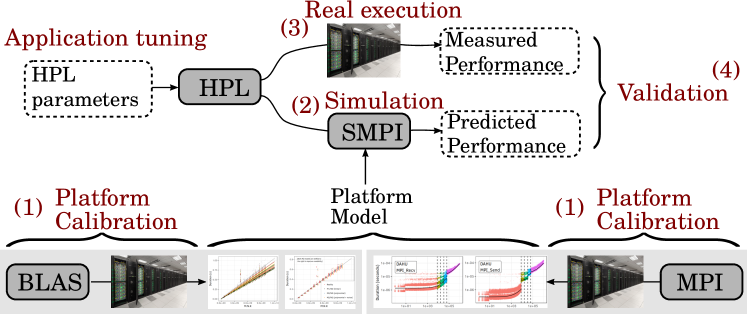
Figure 2: Experimental and simulation workflow with SMPI.

Figure 2 provides an overview of how performance evaluation studies are conducted with SMPI and in this article. First, a series of benchmarks is conducted on the target machine to calibrate (step 1) the platform model. Once this model is built, the application can be simulated over SMPI (step 2) at low cost to predict performance while varying its parameters (e.g., for application tuning) without resorting to the target machine anymore. This approach should be contrasted with the classical one which solely relies on real executions on the target machine (step 3). In this article, as we are particularly interested in evaluating how accurate the predictions are, we propose an extensive comparison of predicted performance with measured performance (step 4). More precisely, we show in Sections 3.4- 4 that predictions are particularly faithful for HPL provided the platform is calibrated with care (steps 1-4) and we show in Section 5 how specific characteristics of HPL can be studied in simulation by slightly varying and extrapolating the platform model (steps 1-2).

3.2 Emulating HPL

⬇

#define HPL_dgemm(layout, TransA, TransB, M, N, K, \

alpha, A, lda, B, ldb, beta, C, ldc) ({ \

double size = ((double)M)*((double)N)*((double)K); \

double expected_time = 1.029e-11*size + 1.981e-12; \

smpi_execute_benched(expected_time); \

})

Figure 3: Non-intrusive macro replacement with a very simple performance model.

HPL relies heavily on BLAS kernels such as dgemm (for matrix-matrix multiplication). Since these kernels’ output does not influence the control flow, simulation time can be reduced considerably by substituting these function calls with a performance model of the respective kernel. Figure 3 shows an example of this macro-based mechanism that allows us to keep HPL code modifications to an absolute minimum. The (1.029e-11) value represents the inverse of the flop rate for this compute kernel and is obtained by benchmarking the target nodes. The kernel’s estimated duration is calculated based on the given parameters and passed on to smpi_execute_benched that advances the simulated clock of the executing rank by this estimate. Skipping compute kernels makes the content of output variables invalid, but in simulation, only the application’s behavior and not the correctness of computation results are of concern. These minor modifications to the original source code (HPL comprises 16K lines of ANSI C over 149 files, our modifications only changed 14 files with 286 line insertions and 18 deletions) enabled us to simulate the configuration used for the Stampede cluster in 2013 for the TOP500 ranking (see Table 1) in less than 62 hours and using $19\text{\,}\mathrm{GB}$ on a single node of a commodity cluster (instead of $120\text{\,}\mathrm{TB}$ of RAM over a 6006 node supercomputer). Further speed-up could probably be obtained by modifying HPL further, but our primary interest in this article is on the prediction quality.

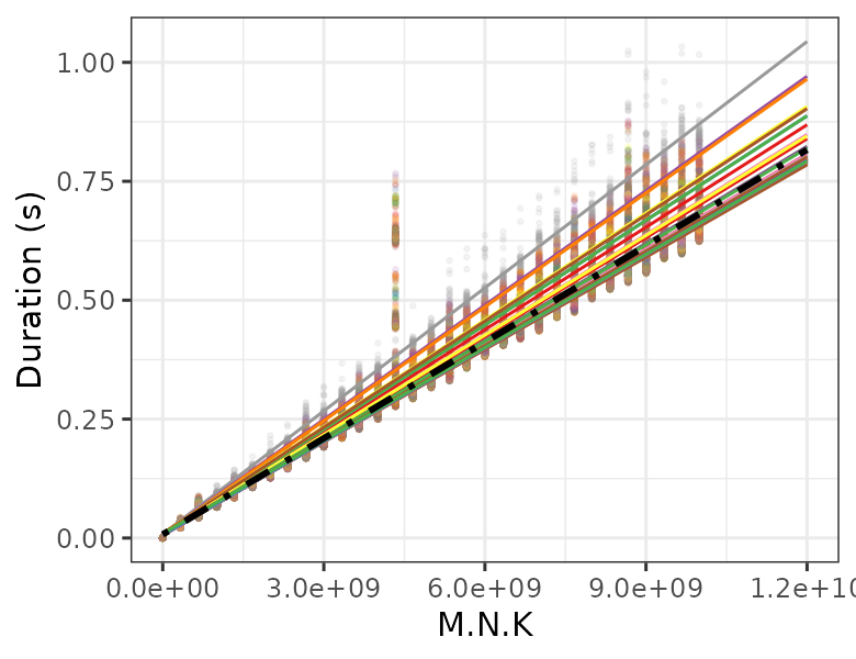
(a) dgemm heterogeneity

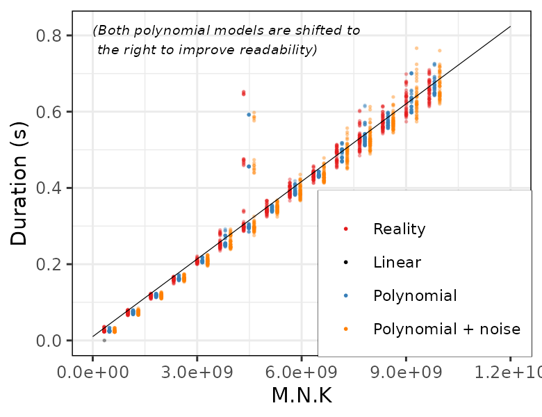
(b) dgemm model

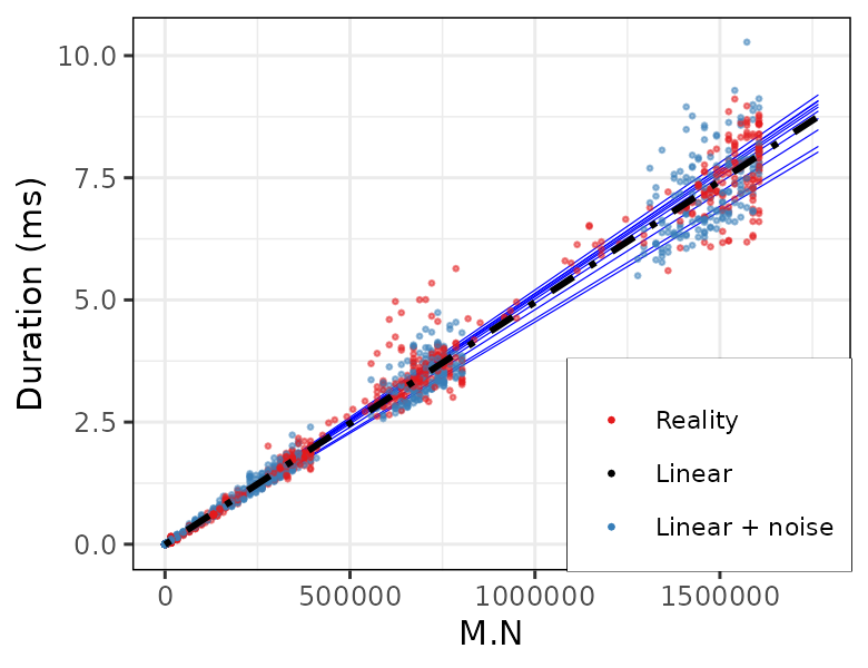
(c) HPL_dlatcpy model

Figure 4: Illustrating the realism of modeling for BLAS and HPL functions.

Most BLAS kernels have several parameters from which a straightforward model can generally easily be identified (e.g., proportional to the product of the parameters), but refinements including the individual contribution of each parameter as well as the spatial and temporal variability of the operation are also possible. In the following, all the simulations have been done with the following model for the dgemm kernel:

$$\begin{split}\text{For each processor $p$, }\textsf{dgemm}_{p}(M,N,K)\sim\mathcal{H}(\mu_{p},\sigma_{p})\\ \begin{cases}\mu_{p}&=\alpha_{p}MNK+\beta_{p}MN+\gamma_{p}MK+\delta_{p}NK+\epsilon_{p}\\ \sigma_{p}&=\omega_{p}MNK+\psi_{p}MN+\phi_{p}MK+\tau_{p}NK+\rho_{p}\end{cases},\end{split}$$ (1)

where $\mathcal{H}(\mu,\sigma)$ denotes a half-normal random variable with parameters $\mu,\sigma$ accounting for the expectation and the standard deviation. The dependency on $p$ allows to account for platform heterogeneity (since $\alpha_{p},\beta_{p},\dots,\rho_{p}$ can be specific to each node), i.e., the aforementioned spatial variability. Figure 4(a) illustrates the importance of distinguishing between nodes: each color and each regression line under a simple linear model corresponds to a different cpu, whereas the black dotted line corresponds to a regression line over all the nodes. Figure 4(b) illustrates the gain brought by a fully polynomial model (blue) over a simple linear model (black) for a given node. Indeed, for $M.N.K\approx 4.5\times 10^{9}$ some duration are systematically higher regardless of the node. In this particular set of experiments the corresponding combination of $M,N,K$ corresponds to some particular (e.g., tall and skinny) matrix geometry which are better handled by a full polynomial model. Last, the $\sigma_{p}$ parameter allows to account for (short-term) temporal variability, i.e., to model the fact that the duration of two successive calls to dgemm with the same parameters $M,N,K$ are never identical. Modeling this variability is important as it may propagate through the communication pattern of the application (late sends and late receives). Figure 4(b) illustrates the gain brought by modeling this variability (orange). The rationale for using a half-normal distribution rather than a normal distribution stems from the natural positive skewness of compute kernel duration. This model is much more complex than the simple deterministic one used in Figure 3 but, as we will explain, this complexity is key to obtain good performance prediction[5]. There are four other BLAS kernel (e.g., daxpy) and a few HPL kernels (often related to memory management) but their total duration represents a negligible fraction of the overall execution time, which have been modeled with a simple deterministic and homogeneous model such as $\texttt{{daxpy}}(N)=\alpha N+\beta$ or $\texttt{{HPL\_dlatcpy}}(M,N)=\alpha M.N+\beta$ (see Figure 4(c)).

3.3 Experimental Setup

To evaluate the soundness of our approach, we compare several real executions of HPL with simulations using the previous models. We used the Dahu cluster from the Grid’5000 testbed. It has 32 nodes connected through a single switch by $100\text{\,}\mathrm{Gbit}\text{\,}{\mathrm{s}}^{-1}$ Omnipath links. Each node has two Intel Xeon Gold 6130 CPUs with 16 cores per CPU, and we disabled hyperthreading. We used HPL version 2.2 compiled with GCC version 6.3.0. We also used the libraries OpenMPI version 2.0.2 and OpenBLAS version 0.3.1. Unless specified otherwise, HPL executions were done using a block size of 128, a matrix of varying size (from $50000$ to $500000$), one single-threaded MPI rank per core, a look-ahead depth of 1, and the increasing-2-ring broadcast with the Crout panel factorization algorithms as this is the combination that led to the best performance overall. Although this machine is much smaller than top supercomputers, faithfully simulating an HPL execution with such settings is quite challenging.

• We used one rank per core to obtain a higher number (1024) of MPI processes. This configuration is more difficult than simulating one rank per node, as (1) it increases the amount of data transferred through MPI, and (2) the performance is subject to memory interference and network heterogeneity (intra-node communications vs. inter-node communications).

• We used a much smaller block size than what is commonly used, which leads to a higher number of iterations and hence more complex communication patterns.

• We used relatively small input matrices, which reduces the makespan and makes good predictions harder to obtain.

3.4 A First Validation

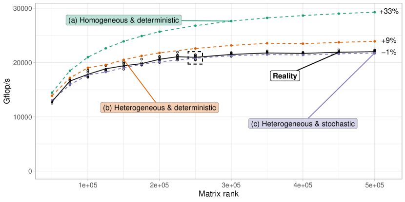
NB	$128$
P$\times$Q	32$\times$32
PFACT	Crout
RFACT	Right
SWAP	Binary-exch.
BCAST	2 Ring
DEPTH	1

Figure 5: HPL performance: predictions (dashed lines) vs. reality (solid lines).

We now present a first quantitative comparison of the prediction with the reality on a typical scenario. We report in Figure 5 the $\mathrm{GFlop}\text{\,}{\mathrm{s}}^{-1}$ rate reported by HPL when varying the matrix size $N$. Real executions are depicted in solid black, and the natural variability of the overall performance is illustrated by reporting eight runs of HPL for each matrix size. The dashed line (a), on top, is our first attempt to simulate HPL with the naive model (homogeneous and deterministic for both the kernels and for the network) illustrated in Figure 3. This model overestimates HPL performance by more than $30\text{\,}\mathrm{\char 37\relax}$. Modeling the heterogeneity of dgemm (i.e., introducing the dependency on $p$ for dgemm as done in Eq (1) but without the temporal variability induced by $\sigma_{p}$) increases significantly the realism of the simulation as the performance is then overestimated by only $9\text{\,}\mathrm{\char 37\relax}$ (dashed line (b)). Finally, we found that adding the temporal variability is the key ingredient to obtain the last bit of realism. The prediction using the full-fledged model (dashed line (c)) is extremely close to reality as it slightly underestimates the performance by less than $5\text{\,}\mathrm{\char 37\relax}$ and even as little as $1\text{\,}\mathrm{\char 37\relax}$ for the larger matrices.

As illustrated in Figure 5 and explained in our previous work[5], accurate predictions require careful modeling of both spatial and temporal variability, as they appear to have a very strong effect on HPL performance. Somehow, this is expected since HPL is an iterative program that synchronizes through the broadcast of factorization panels. A single slower or late process will eventually delay all the other ones. In the scenario presented in Figure 5, a large fraction of the overall execution time is spent in MPI communications but foremost in synchronizations (induced by late sends and let receives) rather than in actual data transfers. As a consequence, careful modeling of computations is essential, but careless modeling of the network was enough to obtain good predictions. This article presents an extensive (in)validation study that demonstrates the importance of careful modeling of the whole platform.

3.5 Experiment Time Frame

This validation study has been carried out over several years (from 2018 to 2020). Despite our efforts to keep the experimental setup stable for the sake of reproducibility, the platform has evolved. The Linux kernel had a minor update, from version 4.9.0-6 to version 4.9.0-13, and the BIOS and firmware of the nodes have been upgraded. During this time frame, the cluster has also suffered from hardware issues, like a cooling malfunction on four of its nodes and several faulty memory modules that had to be changed. This malfunction had an enormous impact on the performance of HPL, which significantly complicated our validation study but also makes it more meaningful as it has been conducted on a particularly challenging setup.

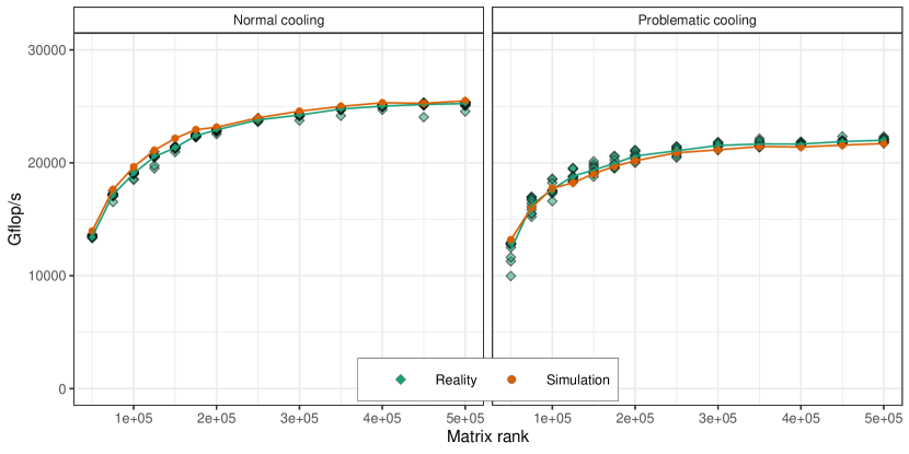
NB	$128$
P$\times$Q	32$\times$32
PFACT	Crout
RFACT	Right
SWAP	Binary-exch.
BCAST	2 Ring
DEPTH	1

Figure 6: HPL performance: predictions vs. reality (effect of the cooling issue on the nodes dahu-{13,14,15,16}).

Our simulation approach makes it possible to predict the performance of HPL for a new platform state by merely making a new calibration whenever a significant change is detected. This ability to reflect in simulation a platform change is illustrated in Figure 6 which, similarly to Figure 5 (acquired in March 2019), showcases the influence of matrix size on the performance but at different periods. The left plot represents the normal state of the cluster (in September 2020), whereas the right plot has been obtained (in March-April 2019) when 4 of the 32 nodes had a cooling issue which lowered their performance by about 10%. In all cases, we consistently predict performance within a few percent and performing a new dgemm calibration on these four nodes was all that was needed to reflect this platform change in the simulation.

This result illustrates both the faithfulness of our simulations and a potential use case for predictive simulations: a discrepancy between the reality and the predictions can sometimes indicate a real issue on the platform (similar situations have already been reported in[1]).

4 Comprehensive Validation Through HPL Performance Tuning

This section reports a few typical performance studies involving HPL through both real experiments and simulations. The comparison of both approaches allows us (1) to cover a broader range of parameters than solely matrix size as done in our earlier work, (2) to evaluate how faithful to reality our simulations are even in suboptimal configurations, and (3) to report the main difficulties encountered when conducting such a study.

4.1 Evaluating the Influence of the Geometry

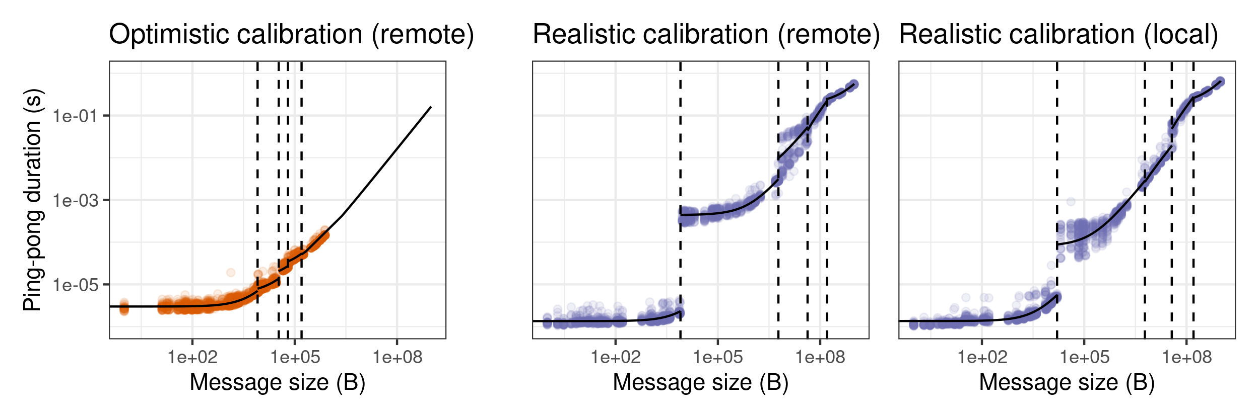
(a) Illustrating the effect of the two MPI calibration methods.

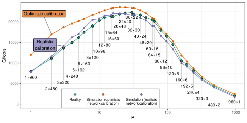
N	$250000$
NB	$128$
P$\times$Q	960
PFACT	Crout
RFACT	Right
SWAP	Binary-exch.
BCAST	2 Ring
DEPTH	1

(b) HPL performance: predictions vs. reality (testing all the possible geometries for 960 MPI ranks).

Figure 7: The first (optimistic) network calibration gave poor predictions for very elongated geometries while the improved calibration provides perfect predictions.

Figure 7(b) illustrates the influence on the performance of the geometry of the virtual topology (P and Q) used in HPL. As expected, geometries that are too distorted lead to degraded performance. All the HPL parameters were fixed (matrix rank is fixed to $250000$ and the other parameters are the same as in Section 3.4) except for the geometry as we evaluate all the pairs (P, Q) such that $\texttt{{P}}\times\texttt{{Q}}=960$. We used only 30 nodes instead of 32 to cover a larger number of geometries, as $960$ has more divisors than $1024$.

As in all our previous studies, we report both the predicted performance and the one measured in reality. Like the comparisons presented in the previous section, the simulation was done with the dgemm model from Eq (1) (stochastic, heterogeneous, and polynomial) and the simplest linear models for the other kernels. In our first simulation attempt that relied on a relatively simple network model (deterministic yet piecewise-linear to account for protocol switch) depicted on the leftmost plot of Figure 7(a), we obtained the unsatisfying orange line on top of Figure 7(b) for the prediction. The simulations with the smallest value of P had relatively large prediction errors, with a systematic over-estimation that reaches up to +50% for the $1\times 960$ and $2\times 480$ geometries. A qualitative comparison of the execution traces obtained in reality and simulation showed that the broadcast phases’ duration was greatly underestimated in simulation. We found out that with such elongated geometries, the message size is significantly larger than what we had used in our calibration, and the performance surprisingly and significantly drops for such size (compare with the rightmost plots of Figure 7(a) for messages larger than $160\text{\,}\mathrm{MB}$). This performance drop is explained by poor optimization of the DMA locking mechanism in the Infiniband network layer[10]. A similar performance drop also happens for intra-node communications that poorly manage the caches above a given size. Furthermore, the communication patterns generated by HPL during the ring broadcast are significantly impacted by the busy waiting of HPL that intensively calls MPI_Probe and dgemm on small sub-matrices. Our initial procedure for calibrating the network did not capture this phenomenon since we did not inject any additional CPU load.

We addressed this problem by improving our network calibration procedure: (1) we use a distinct model for local and remote calibrations, (2) we sample the message sizes in a larger interval (up to $2\text{\,}\mathrm{GB}$ instead of only $1\text{\,}\mathrm{MB}$), and (3) we add calls to dgemm and MPI_Iprobe between each call to MPI_Send and MPI_Recv. The goal was to make the calibration environment more similar to what happens in HPL. The resulting network model is illustrated in the rightmost plots of Figure 7(a). This more realistic network model solved every previous misprediction and allows us to produce very faithful simulations (purple line on Figure 7(b)), which are now a few percent of the reality regardless of the geometry. This figure also illustrates the influence of the geometry on overall performance since there is almost a factor of ten between the worst configuration ($960\times 1$) and the best one ($30\times 32$). Although it is not surprising to see that the geometries which are as square as possible lead to better performance as they minimize the overall amount of data movements, it is interesting to observe the asymmetric role of P and Q in the overall performance (smaller values for P lead to better performance) and which can be explained by the structure of the collective operations but requires a close look at the code.

4.2 Optimizing the HPL Configuration Through a Factorial Experiment

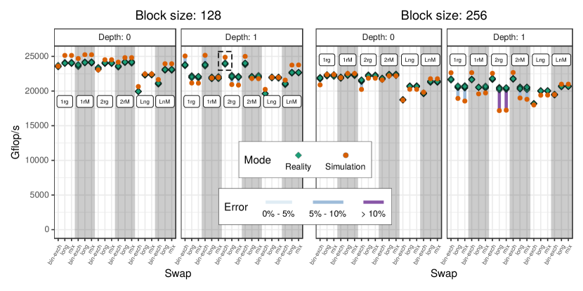
Figure 8: Influence of HPL configuration on the performance (factorial experiment).

Although geometry is among the most important parameter to tune, six other parameters control the behavior of HPL. In Figure 8, we compare the performance reported by HPL when fixing the matrix rank to $250000$ and varying the following parameters: block size (128 or 256), depth (0 or 1), broadcast (the six available algorithms), swap (the three available algorithms). The geometry was fixed to $\text{P}\times\text{Q}=32\times 32=1024$ as it is optimal (the simpler calibration procedure and the network model depicted on the leftmost plot of Figure 7(a) were thus used). The parameters pfact and rfact (panel factorization) were respectively fixed to Crout and Right, as they had nearly no influence on HPL performance in our early experiments.

Figure 8 depicts the 72 parameter combinations we tested. Parameters have been reorganized based on their influence on performance to improve readability. The boxed configuration corresponds to the one boxed in Figure 5. These parameters account for up to $30\text{\,}\mathrm{\char 37\relax}$ of variability in the performance, which is less important than the geometry but is still quite significant. For 61 of them, the prediction error is lower than $5\text{\,}\mathrm{\char 37\relax}$. Only two combinations have shown a large error of approximately $15\text{\,}\mathrm{\char 37\relax}$, obtained with a block size of 256, a depth of 1, the 2-ring broadcast algorithm, and either the long or the mix swap algorithm. This demonstrates the soundness of our approach, as our predictions are reasonably accurate most of the time. This experiment confirms that, although the prediction of HPL performance for a given parameter combination has a systematic bias, the error remains within a few percent most of the time. Therefore, this surrogate is good enough for parameter tuning and should be considered when preparing a large-scale run.

While testing all the parameter combinations is the safest method to discover the combination that provides the highest performance, its cost can be prohibitive due to the high number of combinations. An alternative often used in practice is to explore only a small subset of the parameter space and to analyze variance (ANOVA) to identify the parameters with the more substantial effect on performance and then select the appropriate combination. We applied this procedure on samples of both datasets (the one obtained from real runs and the one obtained in simulation). In both cases, the two parameters with the highest effect were the block size NB and the depth, as shown in Figure 8, followed by bcast and swap. The best combinations selected in both cases were also identical, demonstrating once again the faithfulness of our simulation approach and how it can be used to reduce the experimental cost of parameter tuning.

4.3 Conclusion

Accurately predicting the performance of an application is not a trivial task. Discrepancies between reality and simulation can be multiple: the platform may have changed (e.g., the cooling issue that affected four nodes in Section 3.5), the model could be inaccurate (e.g., the homogeneous and deterministic dgemm model is too simple as in[5]) or not correctly calibrated (e.g., the calibration procedure does not cover the appropriate parameter space, or the experimental conditions are too different as in Section 4.1). As expected in any serious investigation of model validity, our validation study is not a mere collection of positive cases. Instead, it is the result of a thorough (we extensively covered the HPL parameter space) attempt to invalidate our model as well as explanations on how we did so. By meticulously overcoming each of these issues, we have demonstrated the ability of our approach to produce very faithful predictions of HPL performance on a given platform.

5 Sensibility Analysis in What-if Scenarios

We have shown that many typical HPL case studies could be conducted in simulation. However, their conclusions (optimal geometry and parameters) are specific to the cluster we used and they require a precise model of several aspects of the target cluster, which may not be possible at early experimental stages. In particular, only a few cluster nodes may be available at first and the whole cluster model should then be constructed from a limited set of observations and carefully extrapolated. This section shows how typical what-if simulation studies should be conducted given such uncertainty. Section 5.1 presents a generative model of node performance that can easily be fit from daily measurements and used to produce a similar platform. This model is used to quantify the importance on overall performance of temporal variability of the dgemm kernel in Section 5.2 and of spatial variability of nodes in Section 5.3. In particular, we show how to study the efficiency of a simple slow node eviction strategy. Finally, we study in Section 5.4 the influence of the physical network topology on overall performance. Most of these studies are particularly difficult to conduct through real experiments because of the difficulty to finely control the platform.

5.1 A Generative Model of Node Performance

As we have seen in Section 4, the performance of nodes exhibits several kinds of variability: i) a spatial variability (between nodes) ii) a “short-term” temporal variability (the one experienced within an HPL run) but also iii) a “long term” temporal variability (from a day to another). As illustrated in Section 3.4, accounting for the first two kinds of variability is essential but during our investigation of the simulation validity, which spanned over several months, we also had to deal with the fact that the node performance from a day to another could significantly vary, thereby making our comparisons between a real experiment and the simulation driven by model obtained with past measurements sometimes irrelevant.

This section explains how all sources of variability can be accounted for in a single unified model. From our observations, we assume that on a given node $p$ and a given day $d$, the duration of the dgemm kernel can be modeled as follows:

$$\forall M,N,K,\textsf{dgemm}_{p,d}(M,N,K)\sim\mathcal{H}(\alpha_{p,d}MNK+\beta_{p,d},\,\,\gamma_{p,d}MNK)\\$$ (2)

Compared to the model (1), this model includes the daily variability but drops the complexity of a full-fledged polynomial. Such complexity may be important whenever trying to model a particular platform. However, when performing sensibility analysis, a simpler model is preferred, especially as not all terms of the polynomial may be statistically significant. In this model, the short-term temporal variability stems from the $\gamma_{p,d}$ term while the average performance of the node stems from the $\alpha_{p,d}$ and $\beta_{p,d}$ terms, which we gather in a single 3-dimensional vector

$$\mu_{p,d}=(\alpha_{p,d},\beta_{p,d},\gamma_{p,d}).$$ (3)

Now, since every machine is unique it is natural to assume that for each machine:

$$\forall d,\mu_{p,d}\sim\mathcal{N}(\mu_{p},\Sigma_{T})$$ (4)

In this model, $\mu_{p}$ accounts for the average performance of the machine $p$, while $\Sigma_{T}$ accounts for its day-to-day variability. From our observation we had no particular reason to assume that this variability was different from a machine to another, hence, $\Sigma_{T}$ is not indexed by $p$ but global to all machines. However, the parameters $\alpha_{p,d},\beta_{p,d},\gamma_{p,d}$ are generally correlated to each others, hence $\Sigma_{T}$ is full covariance matrix to account for interactions. The choice of a Normal distribution is natural since it is the simpler distribution that accounts for a specific mean and variance, but we will discuss its relevance later in this section.

Finally, we need to account for the spatial variability, which we propose to model as follows:

$$\forall p,\mu_{p}\sim\mathcal{N}(\mu,\Sigma_{S})$$ (5)

Again, in such a model $\mu$ accounts for the machines’ average performance while $\Sigma_{S}$ accounts for the (weak) heterogeneity. This hierarchical model is depicted in Figure 9. The shaded node represents observed variables and diamond node represents deterministic variables, while non-shaded nodes represent latent variables. The solid node is the variable which is estimated when conducting (in)validation studies while the dashed ones are useful when conducting sensibility analysis and extrapolating to an hypothetical cluster.

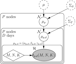
Figure 9: Generative model of kernel duration accounting for the spatial ($\Sigma_{S}$), long-term ($\Sigma_{T}$) and short-term variability ($\gamma_{p,d}$).

The relevance of model (2) has already been illustrated in Section 3.4,  3.5, and 4 but the relevance of models (4) and (5) requires some attention. Figure 10(a) represent the empirical distribution of $\mu_{p,d}=(\alpha_{p,d},\beta_{p,d},\gamma_{p,d})$ (the result of the linear regression) for the 32 nodes of the Dahu cluster on 40 different days from November 2019 to February 2020. The distribution for each node appears approximately normal and passed a Shapiro-Wilk normality test. Although the distribution of the $\beta_{p,d}$ appears slightly skewed toward larger values and one of the nodes (the one with the larger $\alpha_{p,d}$) stands out, there is no good reason for using a more complex distribution than a Gaussian one. Although the correlation between $\alpha$, $\beta$, and $\gamma$ is very weak, it appeared to be statistically significant (most ellipses are slightly tilted toward North-East), hence a full variance matrix is needed (at least for $\Sigma_{T}$).

yReal data  

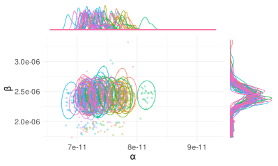
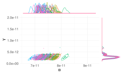
(a) Distribution of $\alpha$, $\beta$, and $\gamma$ (observations on $2\times 32$ CPUs from November 2019 to February 2020).

Synthetic data  

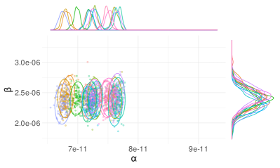
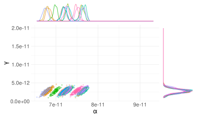
(b) Distribution of $\alpha$, $\beta$, and $\gamma$ (synthetic data for 16 CPUs).

Figure 10: Distribution of the regression parameters for around 20 dgemm calibrations made on each of the 32 nodes. Each color/ellipse corresponds to a different CPU.

yReal data  

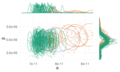
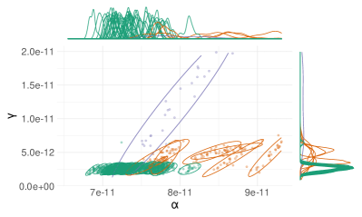
(c) Distribution of $\alpha$, $\beta$, and $\gamma$ (observations on $2\times 32$ CPUs from October to November 2019).

Synthetic data  

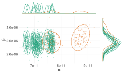
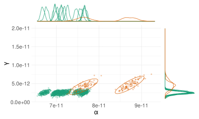
(d) Distribution of $\alpha$, $\beta$, and $\gamma$ (synthetic data for 16 CPUs).

Figure 11: Same as Figure  11, except that 4 of these nodes had a cooling problem, leading to longer and more variable durations.

Table 2: $R^{2}$ values obtained with the linear regressions for dgemm durations, with both the linear and polynomial models.

	Linear	Polynomial
per host and day ($\mu_{p,d}$)	$[0.9842,0.9994]$	$[0.9958,0.9998]$
per host ($\mu_{p}$)	$[0.9960,0.9971]$	$[0.9994,0.9997]$
global ($\mu$)	$0.9963$	$0.9996$

Although fitting a full polynomial model for each day and each processor provides the best predictions it is important to understand that even cruder models are quite good. Table 2 provides indication about the quality of the prediction (the coefficient of determination $R^{2}$, which is comprised between 0 and 1, with 1 indicating a systematically perfect prediction) for the 32 Dahu nodes over the November 2019 to February 2020 period. Regardless of the model complexity (linear/polynomial) and of the granularity of the regression (global, per host, per host and day) the model quality is excellent and above $0.99$, so it could appear that there is no need for a complex model. Yet, we have seen in Section 3.4 that a simple and global linear model of dgemm which is yet an excellent microscopic model ($R^{2}=0.9963$) fails to provide good macroscopic prediction of HPL. The spatial variability is essential, just like the short-term and daily variability, which is why modeling the variability of $\mu_{p,d}$ is key. Last, we recall that if a full polynomial model (with 10 parameters as in (1) instead of 3 as in (2)) is particularly suited to predict the performance of a specific machine and day, it is inadequate to extrapolate performance in general as the covariance matrices $\Sigma_{T}$ and $\Sigma_{S}$ would then have $10\times 9/2=45$ parameters instead of $3$. This is why in the following, we opt for a simpler linear model.

It is easy to estimate $\mu_{p}$ and $\Sigma_{T}$ by averaging over the $\mu_{p,d}$ of each node, and then to estimate $\mu$ and $\Sigma_{S}$ by averaging over all the nodes. This moment-matching method is simple and provides very good estimates for $\mu$, $\Sigma_{T}$, and $\Sigma_{S}$ because we have enough measurements at our disposal and because it is particularly suited to the Gaussian modeling assumption. Should more complex models (e.g., a mixture to account for “outlier” nodes or a SkewNormal distribution to account for the distribution’s skewness) be used, a general Bayesian sampling framework like STAN[11] would be more adapted. Such frameworks allow to easily specify hierarchical generative models like the one presented in Figure 9 and to draw samples from the posterior distribution of $\mu$, $\Sigma_{T}$, and $\Sigma_{S}$, which can be used to generate realistic $\mu_{p,d}$ values for a new hypothetical cluster easily.

Such a process is depicted in Figure 10(b) where hypothetical regression parameters for 16 nodes have been generated. Comparing such synthetic data with the original samples from Figures 10(a) allows us to evaluate the model’s potential weaknesses. Although the orders of magnitude of all parameters and the ellipses are excellent, a few subtle differences are visible. First, the variability of $\alpha_{p}$ seems a bit overestimated (the spread along the x-axis is larger). This can be explained by the fact that one of the nodes seemed to be significantly slower (with much larger $\alpha_{p}$), which artificially increased the spatial variability. Second, as expected from a Gaussian model, the distributions of the $\beta_{p,d}$ are symmetrical whereas there was a slight negative skew in the original samples but this should be of little significance for our study. The distributions of the $\gamma_{p,d}$ however are particularly realistic.

We also illustrate the generality of this model with the data from Figure 10(c). These measurements were obtained from October to November 2019 where the cluster was less stable and where some nodes particularly misbehaved. Three nodes (in orange, hence a total of 6 CPUs) are distinguished from the 28 others (in green) and have lower performance (higher values for $\alpha$, $\beta$, and $\gamma$) and one node (in blue) is particularly unstable. Although this last node may be considered too abnormal to represent anything, it would be reasonable to assume that a larger cluster would present at least the two kinds of behaviors (green for stable nodes, and orange for slower nodes). The higher layer of the model in Figure 9 should then be replaced by a mixture of normal distributions (whose weights would then be sampled from a Dirichlet distribution). Again, hypothetical regression parameters for 16 CPUs have been generated with such a process on Figure 10(d) are very similar, although different, to the original measurements.

Overall this model is therefore of excellent quality and can be used to generate large configurations very easily and evaluate the influence of different kinds of variability on the performance of HPL.

5.2 Influence of dgemm’s Temporal Variability

In Section 3.4, we could highlight the importance of accounting for temporal variability of the dgemm kernel to obtain faithful HPL predictions. To the best of our knowledge, HPL developers and experts are often aware of this influence (or at least suspect it). However, they have never fully quantified it since designing and performing real experiments to evaluate this would be quite difficult. Although increasing this variability wouldn’t be too hard, reducing it would be particularly complicated. This can however easily be done through simulation using the hierarchical model of the previous section. In our experiments, the order of magnitude of the temporal variability with respect to actual performance (i.e., the ratio between $\gamma_{p,d}$ and $\alpha_{p,d}$ in Equation (2)) was around 3%. This may be a “normal” value or could be considered too high and possibly improved by better controlling thread mapping or Operating System noise. Such a task can be quite tedious and knowing how much performance gain can be expected beforehand is thus quite useful. In this section, we study the influence of this variability by generating 10 cluster scenarios using the previous model (as in Figure 11), comprising 1,024 nodes each, but by constraining $\gamma_{p,d}$ to be equal to $\gamma.\alpha_{p,d}$ with $\gamma\in[0,0.1]$, which represents the coefficient of variation of the dgemm kernel. We evaluate the performance of HPL with one multi-threaded MPI rank per node, a block size of 512, a look-ahead depth of 1. We used the increasing-2-ring broadcast with the Crout panel factorization algorithms and $\texttt{{P}}\times\texttt{{Q}}=8\times 32$ and we tested matrix sizes ranging from 100,000 to 500,000. Let us denote by $T(N,C_{i},\gamma)$ the performance of HPL when factorizing a matrix of rank $N$ on cluster $C_{i}$ with a temporal variability of $\gamma$. The overhead for this configuration is the ratio

$$O(N,C_{i},\gamma)=\frac{\mathbb{E}[T(N,C_{i},\gamma)]}{T(N,C_{i},0)}-1.$$

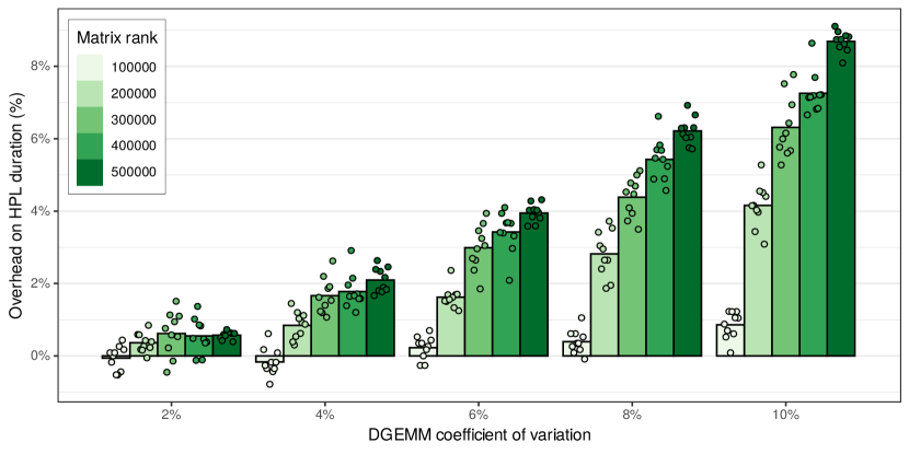
Figure 12: The overhead on HPL duration appears to be linear in dgemm temporal variability. Although it is negligible for small matrices, it severely inflates for larger matrices.

Each bubble in Figure 12 represents one such overhead. For any $\gamma$, this overhead appears to be negligible for small matrices and to increase and flatten when $N$ grows large. In most TOP5000 qualification runs, the matrix is made as large as possible and the overhead would thus appear to grow roughly linearly with $\gamma$. On a new cluster, a simple statistical evaluation of the nodes’ performance using the model of Section 5.1 would thus be a good first diagnosis of whether trying to decreasing temporal variability is a promising tuning target or not.

5.3 Influence of Spatial Variability

Although we showed in Section 3.4 that temporal variability could account for about 9% of performance, spatial variability was even more important as it was responsible for 22% of overhead compared to a fully homogeneous cluster. In practice, the replacement of a few nodes may be possible but such spatial variability is expected and common[12] and a workaround would have to be found. A common approach consists in dropping out a few of the slowest nodes. Indeed, since the matrix is evenly divided between the nodes, the computation inevitably progresses at the speed of the slowest node. However, removing the slowest nodes also decreases the overall processing capability and impacts the virtual topology’s geometry (the P and Q parameters of HPL). Such adjustment is often done by trial and error and is all the more tricky as temporal variability and uncertainty from real experiments come into play. In this section, we show how such a subtle trade-off can be studied in simulation.

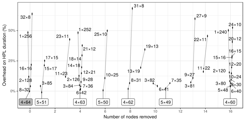
Figure 13: Influence of the number of nodes and of the geometry of the virtual topology on the performance of HPL: $\mathtt{P}\times\mathtt{Q}$ configurations with a small $\mathtt{P}$ perform significantly better then those with a larger $\mathtt{P}$.

Using the model from Section 5.1, we generate 10 mildly heterogeneous 256 node clusters (i.e., where nodes are similar to the ones of our cluster when operating in the normal state as in Figure 10(a)) and we study the performance obtained when removing 1 to 16 of the slowest nodes. When removing nodes, the geometry should be adjusted depending on how the number of remaining nodes decomposes in prime factors. As observed in Figure 7(b), having P $\approx$ Q is generally a good idea to reduce the total amount of communication. However it may be counter-productive for a given broadcast or swap algorithm that serializes communications. Figure 13 shows the overhead for a matrix of rank 250,000 compared to the best performance obtained using the whole cluster. We group the different $\texttt{{P}}\times\texttt{{Q}}$ decompositions and order them by increasing P. Again, we use the 2-Ring and Binary-exch algorithms, which are among the best configurations according to the study of Section 4.2. Each configuration is summarized through the average overhead over the 10 clusters and errorbars represent a 95% confidence interval. It appears that the $4\times 64$ geometry now achieves the best trade-off between the total amount of communications and how well they overlap with each other. The optimal configuration for each number of nodes is boxed in Figure 13. It reveals that there is not much to gain, probably because of the mild spatial heterogeneity of our cluster, but that optimizing the virtual topology is particularly important.

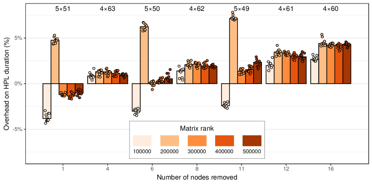
Figure 14: Influence of node removal on performance while taking into account the matrix rank. Due to the mild heterogeneity of these scenarios, evicting nodes brings no benefit.

Figure 14 investigates how this overhead for the best geometry and node selection also depends on the matrix rank. It appears that in this scenario, except for very small matrices, removing nodes cannot help improving performance. Note that the overhead for $5\times\texttt{{Q}}$ configurations with a matrix rank 200,000 appears to behave differently from what happens for other matrix sizes. This surprising effect probably arises from a subtle combination of matrix size and virtual topology. We could indeed observe on our cluster that such configurations had a weakly but significantly worse performance than the other configurations. Such interaction also explains why designing a faithful analytical model of HPL is so difficult and why a full simulation of the whole application is generally required. Although absolute performance should be taken with a grain of salt when studying such subtle effects, they are easily overlooked when conducting real experiments. In this particular small scale mild heterogeneity scenario, there is thus no gain in removing nodes but, as illustrated in Figure 15 where we used a multimodal spatial heterogeneity (as in Figure 11), this may be a relevant approach. This sensibility analysis shows how, for a given supercomputer, a simple statistical evaluation of the spatial heterogeneity allows evaluating whether spatial variability is a promising tuning target or not.

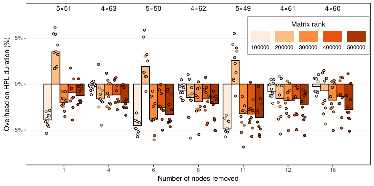
Figure 15: Influence of node removal on performance in a stronger heterogeneity scenario (extrapolation of our test cluster when it had a cooling problem on 4 of its nodes). Removing 6 to 12 nodes our of 256 nodes may bring substantial improvement and such optimization would therefore be worth investigating.

5.4 Influence of the Physical Topology

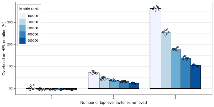
Figure 16: Influence of the physical topology on the overall performance. Up to 2 of the top-level switches can be removed without significantly hurting performances for large matrices. Beyond this point, communications become the main performance bottleneck.

Finally, since virtual topology and communications appear to significantly influence the overall performance, one may wonder how much the physical topology influences the performance. Indeed, several recent articles[13, 14] report that interconnect networks are often oversized compared to the actual need of applications and that turning off some switches could sometimes go completely unnoticed by end-users. In this section we consider ten 256 node clusters with variable node performance (as in Figure 11) interconnected by a 2-level fat-tree and quantify by how much performance degrades when the top-tier switches are gradually deactivated. More formally, we use a (2;32,8;1,N;1,8) fat-tree with $\texttt{{N}}\in\{1,2,3,4\}$. Figure 16 depicts this degradation as a function of matrix size. As one could expect, the impact is more significant for smaller matrix sizes (where the execution is more network bound). Although removing one switch leads to absolutely no visible performance loss, removing two or three switches can have a dramatic effect. Again, such degradation depends on the broadcast and swap algorithms and may be slightly mitigated. To the best of our knowledge, it is the first time such sensibility analysis is conducted faithfully. Generating random node configurations allows avoiding potential bias, in particular against perfectly homogeneous scenarios. We believe such a tool can be quite useful in the earlier steps of a supercomputer design when performing capacity planning to adjust the network capacity to a given cost and power envelope.

6 Discussion

Analytical models are often used for estimating application performance. For instance, Aspen[15] is a domain specific language for specifying formally the characteristics of kernels and combining them to model a whole application. However, such an approach can only provide rough estimates, subtle phenomena like network contention cannot be captured by these models. Another approach for predicting the performance of applications like HPL consists in statistical modeling the application as a whole[16]. By running the application several times with small and medium problem sizes (of a few iterations of large problem sizes) and using simple linear regressions, it is possible to predict its makespan for larger sizes with an error of only a few percent and a relatively low cost. Unfortunately, the predictions are limited to the same application configuration and studying the influence of the number of rows and columns of the virtual grid, or the broadcast algorithms requires a new model and new (costly) runs using the whole target machine. Our attempts to build a black-box analytical model (involving, polynomials, inverse, and logarithms of P and Q) of HPL from a limited set of observations always failed to provide a faithful model with decent prediction and extrapolation capabilities. Furthermore, this approach does not allow studying what-if scenarios (e.g., to evaluate what would happen if the network bandwidth was increased or if node heterogeneity was decreased) that go beyond parameter tuning.

Simulation provides the details and flexibility missing to such a black-box modeling approach. Performance prediction of MPI applications through simulation has been widely studied over the last decades but two approaches can be distinguished in the literature: offline and online simulation.

With the most common approach, offline simulation, a trace of the application is first obtained on a real platform. This trace comprises sequences of MPI operations and CPU bursts and is given as an input to a simulator that implements performance models for the CPUs and the network to derive predictions. Researchers interested in finding out how their application reacts to changes to the underlying platform can replay the trace on commodity hardware at will with different platform models. Most HPC simulators available today, notably BigSim[17], Dimemas[18] and CODES[19], rely on this approach. The main limitation of this approach comes from the trace acquisition requirement. Not only is a large machine required but the compressed trace of a few iterations (out of several thousands) of HPL typically reaches a few hundred MB, making this approach quickly impractical[20]. Worse, tracing an application provides only information about its behavior of a specific run: slight modifications (e.g., to communication patterns) may make the trace inaccurate. The behavior of simple applications (e.g., stencil) can be extrapolated from small-scale traces[21, 22] but this fails if the execution is non-deterministic, e.g., whenever the application relies on non-blocking communication patterns, which is, unfortunately, the case for HPL.

The second approach discussed in the literature is online simulation. Here, the application is executed (emulated) on top of a platform simulator that determines when each process is run. This approach allows researchers to study directly the behavior of MPI applications but only a few recent simulators such as SST Macro[2], SimGrid/SMPI[8] and the closed-source xSim[3] support it. To the best of our knowledge, only SST Macro and SimGrid/SMPI are mature enough to faithfully emulate HPL. In this work, we decided to rely on SimGrid as its performance models and its emulation capabilities are quite solid but the work we present would a priori also be possible with SST. The SST simulator has also been used for uncertainty quantification (UQ)[23], but with a different purpose than what we did in Section 5. Note that the HPL emulation we describe in Section 3.2 should not be confused with the application skeletonization[24] commonly used with SST and more recently introduced in CODES. Skeletons are code extractions of the most important parts of a complex application whereas we only modify a few dozens of lines of HPL before emulating it with SMPI. Some researchers from Intel unaware of our recent work recently applied the same methodology as the one we proposed in[5] to both Intel HPL and OpenHPL in the closed-source CoFluent simulator[25]. To the best of our knowledge, their work reports two faithful predictions for two large-scale supercomputers but without investigating at all the impact of variability, heterogeneity, nor of communications as we do in this article. Finally, it is important to understand that the approach we propose is intended to help studies at the whole machine and application level, not the influence of microarchitectural details as intended by gem5[26] or MUSA[27].

7 Conclusion

HPC application developers implement many elaborate algorithmic strategies whose impact on performance is often dependent on both the input workload and the target platform. This structure makes it very difficult to model and accurately forecast the overall application performance, and many HPC application developers and users are often left with no other option but to study and tune their applications at scale, which can be very time- and resource-consuming. We believe that being capable of precisely predicting an application’s performance on a given platform is useful for application developers and users and will become invaluable in the future as it can, for example, help computing centers with deciding which one of the envisioned technologies for a new machine would work best for a given application or if an upgrade of the current machine should be considered.

Simulation is an effective approach in this context and SimGrid/SMPI has previously been successfully validated in several small-scale studies with simple HPC benchmarks[1, 28]. In an earlier work[5], we have explained how SMPI could be used to efficiently emulate HPL. The proposed approach only requires minimal code modifications and applies to any application whose behavior does not strongly depend on data-dependent intermediate computation results. Although HPL is not a real application, it is quite optimized from an algorithmic point of view and its behavior can be controlled through 6 different parameters (granularity, geometry of the virtual topology, broadcast/swapping/factorization algorithm, and the number of concurrent iterations). HPL features classical optimization techniques such as heavily relying on MPI_Iprobe to overlap communication with computations, making it particularly challenging both in terms of tuning and simulation.

In this article (Section 3 and 4), we present an extensive validation study which covers the whole parameter space of HPL. Our study emphasizes the importance of carefully modeling (1) the platform heterogeneity (not all nodes have exactly the same performance), (2) the short-term temporal variability (e.g., system noise) for compute kernels as it may propagate in communication patterns, and (3) the complexity of MPI (performance often wildly differs between small and large messages and between intra-node and extra-node communications). We show that disregarding any of these aspects may lead to wildly inaccurate predictions even on an application as regular as HPL. By building on a few well-identified micro-benchmarks of the BLAS and MPI, we show that these aspects can be well modeled, which allows us to systematically predict the overall performance of HPL within a few percent. Our experimental results span over two years and we report situations (in Section 3.5 and 4.1) where the simulation helped us to identify performance regression or anomalies incurred by the platform when the prediction did not match the real experiments.

We show (in Section 4) how this faithful surrogate can be used to evaluate the significance of application parameters and tune them accordingly solely through simulations. We also propose a generative model for the compute nodes’ performance that can easily be fit from daily measurements and used to produce synthetic platforms similar to the ones at hand. We show (in Section 5) how this model, which allows us to easily control temporal and spatial variability, can feed our simulations to assess the impact of variability on the performance of the application or of mitigation strategies (e.g., the eviction of the slower nodes). Likewise, the simulation allows to easily assess the influence of the physical network on the overall performance. Most of these what-if studies would be particularly difficult to conduct through real experiments because of the difficulty to finely control the platform. This is to the best of our knowledge one of the first sensitivity analyses of a real HPC code accounting for platform uncertainty.

As future work, building on the effort of SimGrid developers on supporting the emulation of a wide variety of applications with SMPI[29], we also intend to conduct similar studies with other HPC benchmarks (e.g., HPCG[30] or HPGMG[31]), real applications (e.g., BigDFT[32]) and larger infrastructures. As explained in this article, a good model of compute kernels and the MPI library is essential. Thereby, the main challenge for systematic use of our simulation technique now lies in the automation of measurements through well-designed experiments and the automatic detection of when the envisioned models miss essential characteristics of the platform (multi-modal behaviors, heteroscedasticity, discontinuities,…). We intend to provide a fully automatic calibration procedure for MPI as well as for every BLAS function, which would allow us to effortlessly predict the performance of many applications by simply linking against a BLAS-replacement library.

7.1 Acknowledgments

Experiments presented in this paper were carried out using the Grid’5000 testbed, supported by a scientific interest group hosted by Inria and including CNRS, RENATER, and several Universities as well as other organizations (see https://www.grid5000.fr). Last, we warmly thank the SimGrid developers for their help in integrating our contributions and for their early feedback on this work before submission.

This research did not receive any specific grant from funding agencies in the public, commercial, or not-for-profit sectors.

References

- [1] A. Degomme, A. Legrand, G. Markomanolis, M. Quinson, M. S. Stillwell, F. Suter, Simulating MPI applications: the SMPI approach, IEEE Transactions on Parallel and Distributed Systems 28 (8) (2017) 2387–2400. doi:10.1109/TPDS.2017.2669305.
- [2] C. L. Janssen, H. Adalsteinsson, S. Cranford, J. P. Kenny, A. Pinar, D. A. Evensky, J. Mayo, A simulator for large-scale parallel architectures, International Journal of Parallel and Distributed Systems 1 (2) (2010) 57–73, http://dx.doi.org/10.4018/jdst.2010040104. doi:10.4018/jdst.2010040104.
- [3] C. Engelmann, Scaling To A Million Cores And Beyond: Using Light-Weight Simulation to Understand The Challenges Ahead On The Road To Exascale, FGCS 30 (2014) 59–65.
- [4] C. Engelmann, T. Naughton, A network contention model for the extreme-scale simulator, in: Proceedings of the IASTED International Conference on Modelling, Identification and Control (MIC) 2015, ACTA Press, Innsbruck, Austria, 2015. doi:10.2316/P.2015.826-043.
-
[5]
T. Cornebize, A. Legrand, F. C. Heinrich,
Fast and Faithful Performance
Prediction of MPI Applications: the HPL Case Study, in: 2019 IEEE
International Conference on Cluster Computing (CLUSTER), Albuquerque, United
States, 2019.
doi:10.1109/CLUSTER.2019.8891011.
URL https://hal.inria.fr/hal-02096571 - [6] H. W. Meuer, E. Strohmaier, J. Dongarra, H. D. Simon, The TOP500: History, Trends, and Future Directions in High Performance Computing, 1st Edition, Chapman & Hall/CRC, 2014.
- [7] A. Petitet, C. Whaley, J. Dongarra, A. Cleary, P. Luszczek, HPL - a portable implementation of the High-Performance Linpack benchmark for distributed-memory computers, http://www.netlib.org/benchmark/hpl, version 2.2 (February 2016).
- [8] H. Casanova, A. Giersch, A. Legrand, M. Quinson, F. Suter, Versatile, Scalable, and Accurate Simulation of Distributed Applications and Platforms, Journal of Parallel and Distributed Computing 74 (10) (2014) 2899–2917.
- [9] P. Velho, L. Schnorr, H. Casanova, A. Legrand, On the Validity of Flow-level TCP Network Models for Grid and Cloud Simulations, ACM Transactions on Modeling and Computer Simulation 23 (4) (2013) 23.
-
[10]
A. Denis, A High-Performance
Superpipeline Protocol for InfiniBand, in: E. Jeannot, R. Namyst, J. Roman
(Eds.), Euro-Par 2011, Vol. 6853 of Lecture Notes in Computer Science,
Springer, Bordeaux, France, 2011, pp. 276–287.
URL https://hal.inria.fr/inria-00586015 -
[11]
B. Carpenter, A. Gelman, M. D. Hoffman, D. Lee, B. Goodrich, M. Betancourt,
M. Brubaker, J. Guo, P. Li, A. Riddell,
Stan: A probabilistic
programming language, Journal of Statistical Software 76 (1) (2017).
doi:10.18637/jss.v076.i01.
URL https://doi.org/10.18637%2Fjss.v076.i01 - [12] Y. Inadomi, T. Patki, K. Inoue, M. Aoyagi, B. Rountree, M. Schulz, D. Lowenthal, Y. Wada, K. Fukazawa, M. Ueda, M. Kondo, I. Miyoshi, Analyzing and mitigating the impact of manufacturing variability in power-constrained supercomputing, in: SC ’15: Proceedings of the International Conference for High Performance Computing, Networking, Storage and Analysis, 2015, pp. 1–12. doi:10.1145/2807591.2807638.
- [13] E. A. León, I. Karlin, A. Bhatele, S. H. Langer, C. Chambreau, L. H. Howell, T. D’Hooge, M. L. Leininger, Characterizing parallel scientific applications on commodity clusters: An empirical study of a tapered fat-tree, in: SC ’16: Proceedings of the International Conference for High Performance Computing, Networking, Storage and Analysis, 2016, pp. 909–920. doi:10.1109/SC.2016.77.
- [14] P. Taffet, S. Rao, E. León, I. Karlin, Testing the limits of tapered fat tree networks, in: 2019 IEEE/ACM Performance Modeling, Benchmarking and Simulation of High Performance Computer Systems (PMBS), 2019, pp. 47–52. doi:10.1109/PMBS49563.2019.00011.
- [15] K. L. Spafford, J. S. Vetter, Aspen: A domain specific language for performance modeling, in: SC ’12: Proceedings of the International Conference on High Performance Computing, Networking, Storage and Analysis, 2012, pp. 1–11. doi:10.1109/SC.2012.20.
-
[16]
P. Luszczek, J. Dongarra,
Reducing the time to
tune parallel dense linear algebra routines with partial execution and
performance modeling, in: Parallel Processing and Applied Mathematics,
Springer Berlin Heidelberg, 2012, pp. 730–739.
doi:10.1007/978-3-642-31464-3_74.
URL https://doi.org/10.1007%2F978-3-642-31464-3_74 - [17] G. Zheng, G. Kakulapati, L. Kale, BigSim: A Parallel Simulator for Performance Prediction of Extremely Large Parallel Machines, in: Proc. of the 18th IPDPS, 2004.
- [18] R. M. Badia, J. Labarta, J. Giménez, F. Escalé, Dimemas: Predicting MPI Applications Behaviour in Grid Environments, in: Proc. of the Workshop on Grid Applications and Programming Tools, 2003.
- [19] M. Mubarak, C. D. Carothers, R. B. Ross, P. H. Carns, Enabling parallel simulation of large-scale HPC network systems, IEEE Transactions on Parallel and Distributed Systems (2016).
-
[20]
H. Casanova, F. Desprez, G. S. Markomanolis, F. Suter,
Simulation of MPI applications with
time-independent traces, Concurrency and Computation: Practice and
Experience 27 (5) (2015) 24.
doi:10.1002/cpe.3278.
URL https://hal.inria.fr/hal-01232776 - [21] X. Wu, F. Mueller, ScalaExtrap: Trace-based communication extrapolation for SPMD programs, in: Proc. of the 16th ACM Symp. on Principles and Practice of Parallel Programming, 2011, pp. 113–122.
- [22] L. Carrington, M. Laurenzano, A. Tiwari, Inferring large-scale computation behavior via trace extrapolation, in: Proc. of the Workshop on Large-Scale Parallel Processing, 2013.
- [23] J. J. Wilke, K. Sargsyan, J. P. Kenny, B. Debusschere, H. N. Najm, G. Hendry, Validation and uncertainty assessment of extreme-scale hpc simulation through bayesian inference, in: F. Wolf, B. Mohr, D. an Mey (Eds.), Euro-Par 2013 Parallel Processing, Springer Berlin Heidelberg, Berlin, Heidelberg, 2013, pp. 41–52.
- [24] R. F. Bird, S. A. Wright, D. A. Beckingsale, S. A. Jarvis, Performance modelling of magnetohydrodynamics codes, in: M. Tribastone, S. Gilmore (Eds.), Computer Performance Engineering, Springer Berlin Heidelberg, Berlin, Heidelberg, 2013, pp. 197–209.
- [25] G. Xu, H. Ibeid, X. Jiang, V. Svilan, Z. Bian, Simulation-based performance prediction of hpc applications: A case study of hpl, in: 2020 IEEE/ACM International Workshop on HPC User Support Tools (HUST) and Workshop on Programming and Performance Visualization Tools (ProTools), 2020, pp. 81–88. doi:10.1109/HUSTProtools51951.2020.00016.
- [26] J. Lowe-Power, A. M. Ahmad, A. Akram, M. Alian, R. Amslinger, M. Andreozzi, A. Armejach, N. Asmussen, B. Beckmann, S. Bharadwaj, G. Black, G. Bloom, B. R. Bruce, D. R. Carvalho, J. Castrillon, L. Chen, N. Derumigny, S. Diestelhorst, W. Elsasser, C. Escuin, M. Fariborz, A. Farmahini-Farahani, P. Fotouhi, R. Gambord, J. Gandhi, D. Gope, T. Grass, A. Gutierrez, B. Hanindhito, A. Hansson, S. Haria, A. Harris, T. Hayes, A. Herrera, M. Horsnell, S. A. R. Jafri, R. Jagtap, H. Jang, R. Jeyapaul, T. M. Jones, M. Jung, S. Kannoth, H. Khaleghzadeh, Y. Kodama, T. Krishna, T. Marinelli, C. Menard, A. Mondelli, M. Moreto, T. Mück, O. Naji, K. Nathella, H. Nguyen, N. Nikoleris, L. E. Olson, M. Orr, B. Pham, P. Prieto, T. Reddy, A. Roelke, M. Samani, A. Sandberg, J. Setoain, B. Shingarov, M. D. Sinclair, T. Ta, R. Thakur, G. Travaglini, M. Upton, N. Vaish, I. Vougioukas, W. Wang, Z. Wang, N. Wehn, C. Weis, D. A. Wood, H. Yoon, Éder F. Zulian, The gem5 simulator: Version 20.0+ (2020). arXiv:2007.03152.
-
[27]
T. Grass, C. Allande, A. Armejach, A. Rico, E. Ayguadé, J. Labarta,
M. Valero, M. Casas, M. Moreto,
Musa: A multi-level
simulation approach for next-generation hpc machines, in: Proceedings of the
International Conference for High Performance Computing, Networking, Storage
and Analysis, SC ’16, IEEE Press, Piscataway, NJ, USA, 2016, pp. 45:1–45:12.
URL http://dl.acm.org/citation.cfm?id=3014904.3014965 -
[28]
F. C. Heinrich, T. Cornebize, A. Degomme, A. Legrand, A. Carpen-Amarie,
S. Hunold, A.-C. Orgerie, M. Quinson,
Predicting the Energy Consumption
of MPI Applications at Scale Using a Single Node, in: Proc. of the 19th
IEEE Cluster Conference, 2017.
URL https://hal.inria.fr/hal-01523608 - [29] S. Developers, Continuous integration of ECP Proxy Apps, CORAL and Trinity-Nersc benchmarks with SimGrid/SMPI, https://github.com/simgrid/SMPI-proxy-apps/ (2019).
- [30] J. J. Dongarra, M. A. Heroux, P. Luszczek, HPCG benchmark : a new metric for ranking high performance computing systems, Tech. Rep. UT-EECS-15-736, Technion Israel Institute of Technology (2015).
- [31] M. F. Adams, J. Brown, J. Shalf, B. Straalen, E. Strohmaier, S. Williams, Hpgmg 1.0: A benchmark for ranking high performance computing systems, Tech. rep., LBNL (05 2014).
- [32] L. Genovese, A. Neelov, S. Goedecker, T. Deutsch, S. A. Ghasemi, A. Willand, D. Caliste, O. Zilberberg, M. Rayson, A. Bergman, R. Schneider, Daubechies wavelets as a basis set for density functional pseudopotential calculations, Journal of Chemical Physics 129 (2008).