Higgs boson self-coupling constraints from single Higgs, double Higgs and Electroweak measurements

Abstract

We set constraints on the trilinear Higgs boson self-coupling, $\lambda_{3}$, by combining the information coming from the $W$ mass and leptonic effective Weinberg angle, electroweak precision observables, with the single Higgs boson analyses targeting the $\gamma\gamma,\,ZZ^{*},\,WW^{*},\,\tau^{+}\tau^{-}$ and $\bar{b}b$ decay channels and the double Higgs boson analyses in the $b\bar{b}b\bar{b},\,b\bar{b}b\tau^{+}\tau^{-}$ and $b\bar{b}b\gamma\gamma$ decay channels, performed by the ATLAS collaboration. With the assumption that the new physics affects only the Higgs potential, values outside the interval $-1.8\,\lambda_{3}^{\rm SM}<\lambda_{3}<9.2\,\lambda_{3}^{\rm SM}$ are excluded at $95\%$ confidence level. With respect to similar analyses that do not include the information coming from the electroweak precision observables our analysis shows a stronger constraint on both positive and negative values of $\lambda_{3}$.

1 Introduction

With the discovery of the Higgs boson [1, 2, 3, 4], the study of the Higgs boson potential and of the Higgs self-interactions [5] has become of great interest in the scientific community [6]. The shape of the Higgs boson energy potential and the value of the Higgs self-couplings have deep implications on cosmology [7, 8, 9] and on quantum field theory, in particular in connection with gravity [10].

In the Standard Model (SM) the coupling of the quartic term in the Higgs potential, $\lambda$, dictates the trilinear and quadrilinear Higgs self-interactions and its value is related to the Higgs field vacuum expectation value, $v$, and the Higgs boson mass, $m_{\scriptscriptstyle H}$, by $\lambda\equiv\lambda_{3}^{\rm SM}=m_{\scriptscriptstyle H}^{2}/2v^{2}$. Thus, it can be expressed as a function of physically measurable quantities in terms of $G_{F}$ and $m_{\scriptscriptstyle H}$ as $\lambda_{3}^{\rm SM}=G_{F}m_{\scriptscriptstyle H}^{2}\,\sqrt{2}$, where $G_{F}$ is the Fermi coupling constant, linked to $v$ via $v=({\sqrt{2}\,G_{F}})^{-1/2}$, whose value is obtained from the muon lifetime measurement: $G_{F}=1.1663788\times 10^{-5}\,\textrm{GeV}^{-2}$ [11], while $m_{\scriptscriptstyle H}$ is the Higgs boson mass measured from the Higgs boson decay products [12, 13, 14, 15], $m_{\scriptscriptstyle H}=125.14$ GeV.

The Higgs self-interactions affect any observable either at the tree-level or via quantum corrections. In particular, the trilinear Higgs coupling, $\lambda_{3}$, affects the double-Higgs boson production, $pp\to HH$ at the tree-level [5, 16] while both single-Higgs boson production and decay processes are affected at the one-loop level [17]. Going on in the perturbative expansion, i.e. at the two-loop level, $\lambda_{3}$ affects observables with no Higgs bosons as external states, like the electroweak precision observables (EWPO), in particular the $W$ boson mass, $m_{\scriptscriptstyle W}$, and the leptonic effective Weinberg angle $\sin^{2}\theta^{{\rm lep}}_{{\rm eff}}$ [18]. The latter differs from the Weinberg angle $\theta_{W}$ defined in terms of the physical $W$ and $Z$ boson masses through the relation $\cos\theta_{W}=m_{\scriptscriptstyle W}/m_{\scriptscriptstyle Z}$, by a renormalization factor $\kappa^{lep}$ such that $\sin^{2}\theta^{{\rm lep}}_{{\rm eff}}=\kappa^{lep}\sin^{2}\theta_{W}$, where $\kappa^{lep}$ includes all higher order corrections affecting the coupling of the Z boson to leptons.

While the couplings of the Higgs boson to vector bosons and fermions have been measured at the $5\%$ level [19, 20, 21], among the Higgs self-interactions only the trilinear one can be constrained experimentally, although very weakly. Then, it is worth to use all the available experimental information in order to strengthen the constraint on $\lambda_{3}$, albeit under some assumptions. At present the constraint on $\lambda_{3}$ obtained by the ATLAS collaboration combines the information from double Higgs analyses with an integrated luminosity up to $36.1\>{\rm fb}^{-1}$ with single Higgs analyses up to $79.8\>{\rm fb}^{-1}$ reporting that values of $\lambda_{3}$ outside the interval $-2.3\,\lambda_{3}^{\rm SM}<\lambda_{3}<10.3\,\lambda_{3}^{\rm SM}$ are excluded at $95\%$ confidence level (CL) [22]. Instead the CMS collaboration, using the process $pp\to HH\to b\bar{b}\gamma\gamma$ with an integrated luminosity of $137\>{\rm fb}^{-1}$, is able to exclude $\lambda_{3}$ values outside $-3.3\,\lambda_{3}^{\rm SM}<\lambda_{3}<8.5\,\lambda_{3}^{\rm SM}$ at 95 % CL [23].

In this letter we make a further step on the path of strengthening the constraint on $\lambda_{3}$ by combining the public information available on the double and single-Higgs processes from the ATLAS Collaboration with the information coming from the EWPO. We perform a fit to double and single-Higgs production cross sections and Higgs decay channels together with the value of $W$ mass and $\sin^{2}\theta^{{\rm lep}}_{{\rm eff}}$ building a likelihood function of one parameter of interest, $\kappa_{\lambda}$, that measures the deformation of the Higgs trilinear coupling with respect to its SM value, or $\lambda_{3}=\kappa_{\lambda}\lambda_{3}^{\rm SM}$.

The paper is organized as follows. In section 2 we discuss the theoretical framework in which our analysis is inserted. In section 3 the experimental inputs that enter in our analysis are presented and discussed. Section 4 contains the fit procedure we employed, while the next section contains the results of the various fits we perform. Finally we present our conclusions.

2 Theoretical framework

In this section we briefly review some of the results presented in refs.[17, 18, 24] that were used as a basis for our analysis. We are interested in studying a Beyond the Standard Model (BSM) scenario where the dominant effect of an unknown new physics (NP) is concentrated on the modification of the Higgs potential

$$V(H)_{\rm BSM}=\frac{1}{2}m_{\scriptscriptstyle H}^{2}H^{2}+\kappa_{\lambda}\lambda_{3}^{\rm SM}vH^{3}+\kappa_{\lambda 4}\frac{\lambda_{3}^{\rm SM}}{4}H^{4}+\cdots,$$ (1)

where the dots represent higher orders interactions, while at the same time the effects of NP on the other SM couplings are assumed to be negligible. This scenario can be described by a Lagrangian that differs from the SM one only in the scalar potential part that is modified via an (in)finite tower of $(\Phi^{\dagger}\Phi)^{n}$ terms or

$$V^{NP}=\sum_{n=1}^{N}\mathcal{C}_{2n}(\Phi^{\dagger}\Phi)^{n}\,,\qquad\qquad\Phi=\binom{0}{\frac{1}{\sqrt{2}}(v+H)}\,,$$ (2)

with $\Phi$ the Higgs doublet, as shown in the Unitary gauge.

The $\kappa$ factors in eq.(1) can be easily related to the coefficient $\mathcal{C}_{2n}$ in eq.(2). In particular for the trilinear Higgs self-interaction one finds [18]

$$\kappa_{\lambda}=1+2\frac{v^{2}}{m_{\scriptscriptstyle H}^{2}}\,\frac{1}{3}\sum_{n=3}^{N}\mathcal{C}_{2n}\,n(n-1)(n-2)\left(\frac{v^{2}}{2}\right)^{n-2}\,.$$ (3)

We remark that the potential in eq.(2) is assumed to be general, i.e. the coefficients $\mathcal{C}_{2n}$ are not supposed to obey a hierarchy scaling as $\mathcal{C}_{2n+2}\sim\mathcal{C}_{2n}v^{2}/\Lambda_{NP}^{2}$, with $\Lambda_{NP}$ the scale of NP, like in a well-behaved Effective Field Theory (EFT).

The effects induced on the observables by a modified trilinear Higgs self-interaction occur at different orders in the perturbative expansion (tree or loop level) depending on the observable under consideration. When these effects appear for the first time at the loop level, i.e. in single-Higgs processes and EWPO, the modification of the observable induced by the lowest-order contribution can be parametrized as

$$\mathcal{O}_{\rm BSM}=\mathcal{O}_{\rm SM}\,\left(1+(\kappa_{\lambda}-1)C_{1}+(\kappa_{\lambda}^{2}-1)C_{2}\right),$$ (4)

where $\mathcal{O}$ is a generic observable defined in the BSM scenario or in the SM respectively, and $C_{1}$ and $C_{2}$ are finite numerical coefficients, i.e. their values do not depend on $\Lambda_{NP}$.

	$C_{1}$	$C_{2}$
$m_{\scriptscriptstyle W}$	$5.62\times 10^{-6}$	$-1.54\times 10^{-6}$
$\sin^{2}\theta^{{\rm lep}}_{{\rm eff}}$	$-1.56\times 10^{-5}$	$4.55\times 10^{-6}$

Table 1: Values of the coefficients $C_{1}$ and $C_{2}$ for the EWPO.

The values of the $C_{1},\,C_{2}$ coefficients for single-Higgs observables are reported in ref.[17] while those for the EWPO can be found in ref.[18]. Here we use the latest SM theoretical predictions for $m_{\scriptscriptstyle W}$ [25] and $\sin^{2}\theta^{{\rm lep}}_{{\rm eff}}$ [26] to refine the calculation of the latter coefficients. We employ as SM predictions $m_{\scriptscriptstyle W}=80.359\pm 0.06$ GeV and $\sin^{2}\theta^{{\rm lep}}_{{\rm eff}}=0.23151\pm 0.00006$ where the errors reported are obtained combining in quadrature the parametric uncertainties with our estimate of the missing higher order terms [18]. In Table 1 the updated values of the $C_{1},\,C_{2}$ coefficients are presented.

Before concluding this section we want to comment on the total uncertainties that affect our analysis. For any measurement, besides the experimental uncertainty, we take into account a theory uncertainty that can be divided in a part related to the SM prediction and another $\kappa_{\lambda}$-dependent associated to missing higher order terms. The former is usually already included in the experimental analyses while the latter is actually very difficult to estimate. In ref.[17] the $\kappa_{\lambda}$-dependent uncertainty was estimated in terms of the process-dependent coefficient $C_{1}$, however the result of that analysis showed a very mild dependence on this uncertainty. Concerning the $\kappa_{\lambda}$-dependent uncertainty of the EWPO we used the same kind of estimate of ref.[17] finding also in our case a very mild dependence on this uncertainty.

3 Data inputs

In this Section we discuss the experimental inputs we use in the fit. The observables we consider are: the $pp\to HH\to b\bar{b}\gamma\gamma$, the $pp\to HH\to b\bar{b}b\bar{b}$ and the $pp\to HH\to b\bar{b}\tau^{+}\tau^{-}$ production cross sections as measured by the ATLAS collaboration [27, 28, 29, 30]; the measurements of the single-Higgs boson production cross sections including the gluon fusion (ggF), the vector boson fusion (VBF), the associate production (VH) and the $t\bar{t}H$ production modes; the branching fractions of the $H\to\gamma\gamma$, $H\to ZZ$, $H\to W^{+}W^{-}$, $H\to b\bar{b}$ and $H\to\tau^{+}\tau^{-}$ decay channels [19]; the value of the $W$ boson mass from the world average [12, 31, 32, 33, 34, 35, 36, 37]; $\sin^{2}\theta^{{\rm lep}}_{{\rm eff}}$ as estimated in ref.[25] from the average of the LEP [38, 39, 40, 41], SLD [42, 43], Tevatron [44, 45, 46] and LHC [47, 48, 49] data.

The $\sin^{2}\theta^{{\rm lep}}_{{\rm eff}}$ measurements are slightly inconsistent due to a discrepancy at the level of 3$\sigma$ between the LEP and the SLD most accurate measurements, namely the measurement obtained from the forward-backward asymmetry in the $e^{+}e^{-}\to Z\to b\bar{b}$ at LEP and the one obtained from the left-right asymmetry A_LR in $e^{+}e^{-}\to Z\to l^{+}l^{-}$ at SLD. The $\chi^{2}$ of the fit is 11.5 with 5 degrees of freedom. In order to not underestimate the error on the average, from combining discrepant measurements, and to be conservative, we assume that the discrepancy is due to an underestimated systematic error that affects all measurements. Therefore all measurement uncertainties are multiplied by a scaling factor $\kappa=\sqrt{11.5/5}$ such that the $\chi^{2}$ of the fit of the combined measurements equals its expectation value, this in turn consists in multiplying by 1.52 the error of the average computed in ref.[25]: $\sin^{2}\theta^{{\rm lep}}_{{\rm eff}}=0.23151\pm 0.00014$. The single-Higgs boson measurements were taken from the ATLAS collaboration results, nevertheless few measurements were excluded from the fit to extract $\kappa_{\lambda}$. In particular the $t\bar{t}H$ production mode with the $H\to\gamma\gamma$ decay mode was excluded to avoid double counting between this channel and the $pp\to HH\to b\bar{b}\gamma\gamma$ channel, as discussed in ref.[22]. Table 2 summarises all the input measurements used in this work.

Double Higgs-boson production (ATLAS data)
Channel		$\mathcal{L}\,$[fb-1]
$pp\to HH\to b\bar{b}\gamma\gamma$		36.1
$pp\to HH\to b\bar{b}b\bar{b}$		27.5
$pp\to HH\to b\bar{b}\tau^{+}\tau^{-}$		36.1
Single Higgs-boson production (ATLAS data)
Decay Channel	Production Mode	$\mathcal{L}$ [fb-1]
$H\to\gamma\gamma$	ggF, VBF, $WH$, $ZH$	139
$H\to ZZ^{*}$	ggF, VBF, $WH$, $ZH$, $t\bar{t}H$	36.1 - 139
$H\to W^{+}W^{-}$	ggF, VBF, $t\bar{t}H$	36.1
$H\to\tau^{+}\tau^{-}$	ggF, VBF, $t\bar{t}H$	36.1
$H\to b\bar{b}$	VBF, $WH$, $ZH$, $t\bar{t}H$	24.5 - 139
Precision electroweak observables
Observable	Value	Reference
$m_{W}$	$80.379\pm 0.012$ GeV	PDG World Average
$\sin^{2}\theta_{\rm eff}^{lep}$	$0.23151\pm 0.00021$	LEP/SLD/Tevatron/LHC

Table 2: Input measurements used in the present work. For the ATLAS measurements the analysed dataset has been specified being the experiment still on-going and analyses updates on larger datasets are expected in the future.

For the single-Higgs boson production and decay modes, it is conventional to fit data using the production cross section and decay branching fraction signal strengths ($\mu_{i}$,$\mu_{f}$), defined as the ratio between the observed values and their SM expectations:

$$\mu_{i} = \sigma^{\rm observed}_{i}/\sigma^{\rm SM}_{i}\,,~{}~{}~{}~{}~{}~{}~{}~{}~{}~{}~{}i=\mathrm{ggF},\,\mathrm{VBF},\,WH,\,ZH,\,t\bar{t}H$$

$$\mu_{f} = \mathrm{Br}_{H\to f}^{\rm observed}/\mathrm{Br}_{H\to f}^{\rm SM}\,,~{}~{}~{}~{}~{}f=\gamma\gamma,\,ZZ^{*},W^{+}W^{-},\,b\bar{b},\,\tau^{+}\tau^{-}~{}.$$

In this work the signal strengths are taken from ref.[19] where the product $\mu_{i}\times\mu_{f}$ is tabulated for each production and decay mode; the values used in this fit are summarised in Table 3. The fit performed in ref.[19] combines the $ZH$ and the $WH$ channel assuming that the ratio of their cross section equals its SM expectation. Such assumption cannot be made in our case because $\kappa_{\lambda}\neq 1$ affects differently the $WH$ and $ZH$ cross sections. Nevertheless the sensitivity of the $VH$ result is dominated by the $H\to b\bar{b}$ channel where $ZH$ provides the most accurate measurement of the $VH$ signal strength value [50]. In this work the $VH$ signal strength is therefore assigned to $ZH$, the impact of this assumption has been tested assigning the $VH$ signal strength of the $\gamma\gamma$ channel (the second most relevant channel after $H\to b\bar{b}$) to $WH$ and decoupling the $WH$ and $ZH$ signal strengths in the $H\to b\bar{b}$ channel using inputs from ref.[50]. The impact on the result has been found to be negligible. In addition, the signal strength relative to $t\bar{t}H+tH$ of the original paper has been assigned to $t\bar{t}H$ being the $tH$ contribution negligible, and the $VV$ channel indicated in ref.[19] has been assigned to $W^{+}W^{-}$ that dominates the sensitivity. Finally the uncertainties on the signal strengths have been symmetrised by averaging the squares of the positive and negative uncertainties.

$\mu_{i}\times\mu_{f}$	ggF	VBF	$ZH$	$t\bar{t}H$
$\gamma\gamma$	1.03 $\pm$ 0.11	1.31 $\pm$ 0.25	1.32 $\pm$ 0.32	–
$ZZ^{*}$	0.94 $\pm$ 0.11	1.25 $\pm$ 0.46	1.53 $\pm$ 1.03	–
$W^{+}W^{-}$	1.08 $\pm$ 0.19	0.60 $\pm$ 0.35	–	1.72 $\pm$ 0.55
$b\bar{b}$	–	3.03 $\pm$ 1.65	1.02 $\pm$ 0.18	0.79 $\pm$ 0.60
$\tau^{+}\tau^{-}$	1.02 $\pm$ 0.58	1.15 $\pm$ 0.55	–	1.20 $\pm$ 1.00

Table 3: Values of the product $\mu_{i}\times\mu_{f}$ used in the fit procedure. The values corresponds to the product $\sigma\times\mathrm{Br}$ normalised to its Standard Model expectation. Rows span over the decay mode $f$ while colums over the production mode $i$.

The measurements shown in Table 3 are correlated due to the cross contamination of signal events among different production and decay channels and the correlation matrix is provided in Figure 6 of ref.[19]; in the present work only correlations larger than 0.05 are taken into account for simplicity; this choice doesn’t have impact on the final results. The correlation coefficients are shown in Table 4.

	ggF	VBF				$VH$	$t\bar{t}H$
$\rho$	$\tau^{+}\tau^{-}$	$\gamma\gamma$	$ZZ^{*}$	$W^{+}W^{-}$	$\tau^{+}\tau^{-}$	$ZZ^{*}$	$W^{+}W^{-}$	$\tau^{+}\tau^{-}$
ggF
$\gamma\gamma$	0.06	-0.11
$ZZ^{*}$			-0.21			-0.28
$W^{+}W^{-}$				-0.08
$\tau^{+}\tau^{-}$					-0.45
VBF
$\gamma\gamma$			0.07
$VH$
$ZZ^{*}$							-0.07
$t\bar{t}H$
$W^{+}W^{-}$								-0.42

Table 4: Correlation matrix of the signal strength measurements used in the fit. Only elements larger or equal to 0.05 are used in the present fit and are shown in the table. The correlation matrix is symmetric therefore only its upper triangle section is reported.

The determination of constraints on $\kappa_{\lambda}$ has been performed by the ATLAS collaboration in ref.[27] using data from the $pp\to HH$ production measurements, with the $HH$ pair decaying to the final states $b\bar{b}\gamma\gamma$, $b\bar{b}\tau^{+}\tau^{-}$ and $b\bar{b}b\bar{b}$, finding $-5.0<\kappa_{\lambda}<12.0$ ($-5.8<\kappa_{\lambda}<12.0$) at $95\%$ CL in observation (expectation). In that paper only the $HH$ production cross section was parameterised as a function of $\kappa_{\lambda}$ while the decay branching fractions were assumed to be independent from $\kappa_{\lambda}$ and equal to their SM expectation. This assumption was removed in a conference note of the same collaboration [22] where the $HH$ constraints were combined with single-Higgs differential measurements. In the $pp\to HH$ process the $\kappa_{\lambda}$ value has a big impact on the dynamic of the decay products affecting strongly the Higgs-pair invariant mass distribution, therefore it is not possible to extract sensible information from the final result without the information on the likelihood of each channel expressed as a function of $\kappa_{\lambda}$.

The likelihood shapes have been taken from ref.[51, 52]. The shape of the expected and observed likelihood of the combination $HH\to b\bar{b}b\bar{b}$, $HH\to b\bar{b}\gamma\gamma$ and $HH\to b\bar{b}\tau^{+}\tau^{-}$ has been first scanned with 200 points and then interpolated using a third degree polynomial. Continuity of the first and the second derivative has been imposed at each point of the scan. The resulting likelihood function used in the fit procedure is shown in Figure 1.

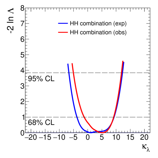
Figure 1: Likelihood function used in the fit procedure from the combination of the $HH\to b\bar{b}b\bar{b}$, the $HH\to b\bar{b}\gamma\gamma$ and the $HH\to b\bar{b}\tau^{+}\tau^{-}$ channels.

4 Fit procedure

The fit procedure is performed by building up a likelihood function as a product of the likelihood function associated to each experimental measurement:

$$\mathcal{L}=\mathcal{L}_{H}\times\mathcal{L}_{HH}\times\mathcal{L}_{m_{W}}\times\mathcal{L}_{\sin^{2}\theta^{\rm lep}_{\rm eff}}$$

The likelihood $\mathcal{L}$ is a function of one parameter of interest $\kappa_{\lambda}$, the ratio: $\Lambda(\kappa_{\lambda})=\mathcal{L}(\kappa_{\lambda})/\mathcal{L}(\hat{\kappa}_{\lambda})$ is used to extract the best fit values and confidence intervals on $\kappa_{\lambda}$, where $\hat{\kappa}_{\lambda}$ is the value that maximises $\mathcal{L}$.

The likelihoods $\mathcal{L}_{H}$, $\mathcal{L}_{HH}$, $\mathcal{L}_{m_{W}}$ and $\mathcal{L}_{\sin^{2}\theta^{{\rm lep}}_{{\rm eff}}}$ are relative to the single Higgs production and decay measurements, the $HH$ production, the $m_{\scriptscriptstyle W}$ and the $\sin^{2}\theta^{{\rm lep}}_{{\rm eff}}$ measurements respectively. The minimisation is performed on the quantity $-2\,{\rm ln}\Lambda$ whose expression is:

$$-2\,{\rm ln}\Lambda=-2\,{\rm ln}\mathcal{L}_{H}-2\,{\rm ln}\mathcal{L}_{HH}-2\,{\rm ln}\mathcal{L}_{m_{\scriptscriptstyle W}}-2\,{\rm ln}\mathcal{L}_{\sin^{2}\theta^{{\rm lep}}_{{\rm eff}}}+2\,{\rm ln}\mathcal{L}(\hat{\kappa}_{\lambda})~{}.$$

The $-2\,{\rm ln}\mathcal{L}_{HH}$ is obtained directly from Figure 1, $-2\,{\rm ln}{\mathcal{L}_{m_{W}}}$ and $-2\,{\rm ln}\mathcal{L}_{\sin^{2}\theta^{{\rm lep}}_{{\rm eff}}}$ are $\chi^{2}$ function built as:

$$-2\,{\rm ln}{\mathcal{L}_{m_{\scriptscriptstyle W}}}=\chi^{2}_{m_{\scriptscriptstyle W}}=\frac{[m_{\scriptscriptstyle W}^{\rm exp}-m_{\scriptscriptstyle W}^{\rm theo}(\kappa_{\lambda})]^{2}}{[\sigma^{2\;exp}_{m_{\scriptscriptstyle W}}+\sigma^{2\,theo}_{m_{\scriptscriptstyle W}}]^{2}}$$

$$-2\,{\rm ln}{\mathcal{L}_{\sin^{2}\theta^{{\rm lep}}_{{\rm eff}}}}=\chi^{2}_{\sin^{2}\theta^{{\rm lep}}_{{\rm eff}}}=\frac{\left[\sin^{2}\theta_{\rm eff}^{\rm lep,exp}-\sin^{2}\theta_{\rm eff}^{\rm lep,theo}(\kappa_{\lambda})\right]^{2}}{\left[\sigma^{2\;{\rm exp}}_{\sin^{2}\theta^{{\rm lep}}_{{\rm eff}}}+\sigma^{2\;{\rm theo}}_{\sin^{2}\theta^{{\rm lep}}_{{\rm eff}}}\right]^{2}}~{}.$$

In this expression the labels ”exp” and ”theo” refer to the experimental and theoretical quantities respectively, while $\sigma$ is the uncertainty on the observable denoted at the subscript. The experimental uncertainties are listed in Table 2 while theoretical uncertainties are discussed in section 2.

The likelihood function $\mathcal{L}_{H}$ contains information from single Higgs boson production and decay measurements, the quantity $-2\,{\rm ln}\mathcal{L}_{H}$ is a $\chi^{2}$ function defined as:

$$-2\,{\rm ln}\mathcal{L}_{H}=\chi^{2}_{H}=\left[\vec{\mu}^{\rm exp}-\vec{\mu}^{\rm theo}(\kappa_{\lambda})\right]^{T}C(\kappa_{\lambda})^{-1}\left[\vec{\mu}^{\rm exp}-\vec{\mu}^{\rm theo}(\kappa_{\lambda})\right]$$

where $\vec{\mu}^{\rm exp}$ is a fifteen dimensional vector containing the measurements $\mu_{i}\times\mu_{f}$ listed in Table 3 and their theoretical expectation as a function of $\kappa_{\lambda}$ described in section 2. The matrix $C(\kappa_{\lambda})^{-1}$ is the inverse of the covariance matrix $C(\kappa_{\lambda})=C^{\rm theo}(\kappa_{\lambda})+C^{\rm exp}$ where $C^{\rm exp}$ is built from the uncertainties shown in Table 3 and the correlation matrix $\rho$ shown in Table 4, while $C^{\rm theo}(\kappa_{\lambda})$ is a diagonal matrix containing the square of the theoretical uncertainties on $\mu_{i}\times\mu_{f}$ due to missing higher order terms as discussed in section 2.

5 Results

The value of $-2\,{\rm ln}\Lambda$ as a function of the $\kappa_{\lambda}$ parameter is shown in the left panel of Figure 2. For positive $\kappa_{\lambda}$ values, i.e. when the interference between the box and the self-coupling diagram in the $pp\to HH$ process is destructive and brings to a sensitivity loss of the double-Higgs channel, all the three measurements ($HH$, single-$H$ and EWPO) show a comparable constraining power, with a stronger impact of the EWPO for low values of $\kappa_{\lambda}$. On the other hand, for negative $\kappa_{\lambda}$ values, the higher statistics of the single-Higgs analyses allows to reach a better constraint on $\kappa_{\lambda}$ while the EWPO have a smaller impact on the result. The fit results are summarised in Table 5.

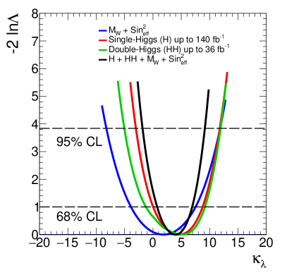
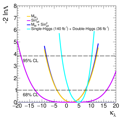
Figure 2: Values of $-2\,\rm{ln}\Lambda$ as a function of $\kappa_{\lambda}$. Left panel: the $m_{\scriptscriptstyle W}+\sin^{2}\theta^{{\rm lep}}_{{\rm eff}}$ combination, the single-Higgs analyses, the double-Higgs analyses and their combination. Right panel: The $m_{\scriptscriptstyle W}$, the $\sin^{2}\theta^{{\rm lep}}_{{\rm eff}}$, their combination and the combination of the single-Higgs and double-Higgs analyses.

observables	best fit	68 % CL interval	95 % CL interval
$\sin^{2}\theta^{{\rm lep}}_{{\rm eff}}$	0.2	-12.8 $-$ 16.2	-18.5 $-{}[>20]$
$m_{W}$	1.8	-3.9 $-$ 7.6	-8.4 $-$ 12.1
$m_{\scriptscriptstyle W}+\sin^{2}\theta^{{\rm lep}}_{{\rm eff}}$	1.8	-3.9 $-$ +7.5	-8.2 $-$ 11.8
$HH$	5.2	-1.2 $-$ +9.2	-5.0 $-$ 11.9
single-$H$	4.6	+0.05 $-$ +8.8	-3.0 $-$ 11.8
Combination	4.0	0.7 $-$ 6.9	-1.8 $-$ 9.2

Table 5: Best fit results, 68% and 95% CL intervals for all measurements used in this work and their combination.

In order to compare the impact on the fit of the two EWPO we disentangle the likelihood functions of $m_{\scriptscriptstyle W}$ and $\sin^{2}\theta^{{\rm lep}}_{{\rm eff}}$ from the $m_{\scriptscriptstyle W}+\sin^{2}\theta^{{\rm lep}}_{{\rm eff}}$ combination and from the combination of single-Higgs plus double-Higgs results, as shown on the right panel of Figure 2. The sensitivity of the EWPO is dominated by the $m_{\scriptscriptstyle W}$ measurement that represents an important addition to the single-Higgs and double-Higgs combination. In order to investigate if this result is due to the intrinsic sensitivity of the EWPO, we have performed the likelihood scan setting all the fit parameters to their SM expectations. For the $HH$ analyses the expected likelihood function has been taken directly from ref.[52], while for the single-Higgs analyses and the EWPO, it has been assumed that the correlation matrix and the fractional error on the fitted parameters don’t change when the parameters move from their observed values to their expected ones. The resulting -2 ln$\Lambda$ functions are shown in Figure 3.

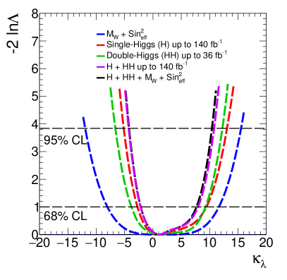
Figure 3: Value of -2  ln$\Lambda$ as a function of $\kappa_{\lambda}$ obtained setting all observables to their SM expectation. The function is shown for the EWPO, the single-Higgs, the double-Higgs observables, the single-Higgs plus double-Higgs combination and the full combination.

The functional shapes of -2 ln$\Lambda$ show that the constraining power of the EWPO is expected to be lower than what observed in data, in fact the full combined -2 ln$\Lambda$ doesn’t show large differences with respect to the combination of only the single-Higgs and double Higgs -2 ln$\Lambda$. From Figure 2 is possible to see that the combined $H$ and $HH$ -2 ln$\Lambda$ has a minimum far from its SM expectation of $\kappa_{\lambda}=1$, while the minimum of the EWPO -2 ln$\Lambda$ is closer to its SM expectation. Therefore the EWPO have an higher impact on the final observed result, in particular at the upper edge of the confidence interval.

6 Conclusion

In this paper we combine the ATLAS data analyses of the single-Higgs and double-Higgs processes with the information coming from the EWPO in order to constraint the Higgs boson trilinear self-coupling modifier $\kappa_{\lambda}=\lambda_{3}/\lambda_{3}^{\rm SM}$. Under the assumption that NP affects only the Higgs potential we find as the best fit value of the trilinear self-coupling modifier $\kappa_{\lambda}=4.0^{+2.9}_{-3.3}$ excluding values outside the interval $-1.8<\kappa_{\lambda}<9.2$ at $95\%$ CL. With respect to analyses where single-Higgs data [22] or double-Higgs data [27] or a combination of both [22] are taken into account, our study shows that the inclusion in the fit of the information coming from the EWPO $m_{\scriptscriptstyle W}$ and $\sin^{2}\theta^{{\rm lep}}_{{\rm eff}}$ gives rise to a stronger constraint on $\kappa_{\lambda}$, in particular on the positive side of the CL interval.

At the moment the information coming from EWPO gives an indication for $\lambda_{3}$ values closer to $\lambda_{3}^{\rm SM}$ than the single and double-Higgs analyses. It is interesting to see if, in the future, with the LHC collaborations analysing larger set of single and double-Higgs data and with possible improvements on the measurement of the $m_{\scriptscriptstyle W}$ from LHC, this different indication will remain in the data.

References

- [1] P.W Higgs, Phys. Lett. 12 (1964) 132
- [2] F. Englert, R. Brout, Phys. Rev. Lett. 13 (1964) 321
- [3] The ATLAS Collaboration, G. Aad et al., Phys. Lett. B 716 (2012) 1
- [4] The CMS Collaboration, S. Chatrchyan et al., Phys. Lett. B 716 (2012) 30
- [5] S. Dawson, S. Dittmaier and M. Spira, Phys. Rev. D 58 (1998) 115012
- [6] B. Di Micco et al., Review in Physics (2020) 100045
- [7] I. Masina, A. Notari, Phys. Rev. D85 (2012) 123506
- [8] D. Buttazzo et al., J. High Energy Phys. 12 (2013) 089
- [9] F.L. Bezrukov, M. Shaposhnikov, Phys. Lett. B (2008) 659
- [10] M. Shaposhnikov, C. Wetterich, Phys. Lett. B (2010) 196
- [11] D. M. Webber et al., Phys. Rev. Lett. 106 (2011) 041803
- [12] P.A. Zyla et al., Prog. Theor. Exp. Phys. (2020) 083C01
- [13] The ATLAS Collaboration, M. Aaboud et al., Phys. Lett. B784 (2018) 345
- [14] The CMS Collaboration, A.M.Sirunyan et al., Phys. Lett. B805 (2020) 135425
- [15] The ATLAS and CMS collaborations, Phys. Rev. Lett. 114 (2015) 191803
- [16] R. Frederix et al., Phys. Lett. B732 (2014) 142
- [17] G. Degrassi et al., J. High Energy Phys. 12 (2016) 080
- [18] G. Degrassi, M. Fedele, P.P. Giardino, J. High Energy Phys. 04 (2017) 155
- [19] The ATLAS collaboration, ATLAS-CONF-2020-027, https://cds.cern.ch/record/2725733
- [20] The ATLAS Collaboration, G. Aad et al. , Phys. Rev. D101 (2020) 012002
- [21] The CMS Collaboration, A. Sirunyan et al., Eur. Phys. J. C79 (2019) 421
- [22] The ATLAS collaboration, ATLAS-CONF-2019-049,https://cds.cern.ch/record/2693958
- [23] The CMS Collaboration, arXiv:2011.12373, https://arxiv.org/abs/2011.12373
- [24] G. Degrassi and M. Vitti, Eur. Phys. J. C80 (2020) 307
- [25] J. Erler, M. Schott, Prog. in Part. and Nuc. Phys. 106 (2019) 68
- [26] I. Dubovyk, A. Freitas, J. Gluza, T. Riemann and J. Usovitsch, JHEP 08 (2019) 113
- [27] The ATLAS collaboration, G. Aad et al., Phys. Lett. B 800 (2020) 135103
- [28] The ATLAS collaboration, M. AAboud et al., J. High Energ. Phys. 2019 (2019) 30
- [29] The ATLAS collaboration, M. AAboud et al., J. High Energ. Phys. 2018 (2018) 40
- [30] The ATLAS collaboration, M. AAboud et al., Phys. Rev. Lett. 122 (2019) 089901
- [31] M. AAboud et al., Eur. Phys. J. C78 (2018) 110
- [32] The ALEPH collaboration, S. Schael et al., Eur. Phys. J. C 47 (2006) 47
- [33] The L3 collaboration, P. Achard et al., Eur. Phys. J. C 45 (2006) 569
- [34] The OPAL collaboration, G. Abbiendi et al., Eur. Phys. J. C 45 (2006) 307
- [35] J. Abdallah et al., Eur. Phys. J. C 55 (2008) 1
- [36] The CDF collaboration, T. Aaltonen et al., Phys. Rev. Lett. 108 (2012) 151803
- [37] The D0 collaboration, V.M. Abazov et al., Phys. Review D89 (2014) 012005
- [38] The ALEPH collaboration, R. Barate et al., Eur. Phys. J. C14 (2000) 1
- [39] The DELPHI collaboration, P. Abreu et al., Eur. Phys. J. C16 (2000) 371
- [40] The L3 collaboration, M. Acciarri et al., Eur. Phys. J. C16 (2000) 1
- [41] The OPAL collaboration, G. Abbiendi et al., Eur. Phys. J. C19 (2001) 587
- [42] The SLD collaboration, K. Abe et al., Phys. Rev. Lett. 84 (2000) 5945
- [43] LEP Electroweak Working Group, SLD Electroweak and Heavy Flavour Groups, ALEPH, DELPHI, L3, OPAL and SLD collaboration, S. Schael, et al., Phys. Rep. 427 (2006) 257
- [44] The D0 collaboration, V.M. Abazov, et al., Phys. Rev. Lett. 120 (2018) 241802
- [45] The CDF collaboration, T. Aaltonen, et al., Phys. Rev. D 93 (2016) 112016 [Addendum: Phys. Rev. D 95 (2017) 119901]
- [46] The CDF and DØ collaboration, T. Aaltonen, et al., Phys. Rev. D 97 (2018) 112007
- [47] The CMS collaboration, A.M. Sirunyan, et al., Eur. Phys. J. C 78 (2018) 701
- [48] The ATLAS collaboration, ATLAS-CONF-2018-037, http://cds.cern.ch/record/2630340
- [49] The LHCb collaboration, R. Aaij, et al., J. High Energy Phys. 11 (2015) 190 The CMS collaboration, A.M. Sirunyan, et al., Eur. Phys. J. C 78 (9) (2018) 701, arXiv:1806.00863 [hep-ex].
- [50] The ATLAS collaboration, G. Aad et al., arXiv:2007.02873, https://arxiv.org/abs/2007.02873
- [51] E. Rossi, CERN-THESIS-2019-320, https://arxiv.org/abs/2010.05252
- [52] E. Rossi, Il Nuovo Cimento C43 (2020) 95