Phase transitions in random mixtures of elementary cellular automata

Abstract

We investigate one–dimensional Probabilistic Cellular Automata, called Diploid Elementary Cellular Automata (DECA), obtained as random mixture of two different Elementary Cellular Automata rules. All the cells are updated synchronously and the probability for one cell to be $0$ or $1$ at time $t$ depends only on the value of the same cell and that of its neighbors at time $t-1$. These very simple models show a very rich behavior strongly depending on the choice of the two Elementary Cellular Automata that are randomly mixed together and on the parameter which governs probabilistically the mixture. In particular, we study the existence of phase transition for the whole set of possible DECA obtained by mixing the null rule which associates $0$ to any possible local configuration, with any of the other $255$ elementary rule. We approach the problem analytically via a Mean Field approximation and via the use of a rigorous approach based on the application of the Dobrushin Criterion. The distinguishing trait of our result is the possibility to describe the behavior of the whole set of considered DECA without exploiting the local properties of the individual models. The results that we find are coherent with numerical studies already published in the scientific literature and also with some rigorous results proven for some specific models.

Keywords: Probabilistic Cellular Automata; Synchronization; Stationary measures; First hitting times; Mean field.

1 Introduction

Probabilistic Cellular Automata (PCA) generalize deterministic Cellular Automata (CA) as discrete–time Markov chains. Despite the simplicity of their stochastic evolution rules, PCA exhibit a large variety of dynamical behaviors and for this reason are powerful modeling tools (see [9] for a general introduction to the topic). In this paper we study the relaxation towards stationarity of a family of one–dimensional PCA, called Diploid Elementary Cellular Automata (DECA), which are defined as Bernoulli mixtures of two Elementary Cellular Automata (ECA) rules [17, 18]. DECA have originally introduced and analyzed in [4] by means of numerical simulations.

By varying the ECA chosen in the mixture, the class of DECA considered in the present manuscript is indeed very rich an includes among the others: the percolation PCA studied in [1] and [16], the noisy additive PCA [11], the Stavskaya’s PCA [13] and the directed animals PCA [5].

The long–time limit of the PCA has been the subject of many numerical and theoretical results in the last fifty years, see for instance [15, 16]. In this paper we focus on the properties of DECA’s stationary states in function of the parameter $\lambda$ governing the Bernoulli mixture. In particular, we study the presence of phase transitions associated to multiple invariant measures.

In case of uniqueness of the invariant measure, a natural questions are related to attractiveness and ergodicity of the system [16]. However, ergodicity will not be the focus of this paper and we just recall that the uniqueness of the invariant measure does not imply ergodicity [2, 8]. We will be interested instead to the structure of the phase diagram of the DECA in relation to the mixing parameter $\lambda$ and to the choice of the two mixed ECA.

A rigorous study of the phase diagram of DECA is possible only for a tiny subset of the ECA rules. For this reason, we thus use a Mean Field (MF) approximation [7, 12] to get a wide overview of the possible behaviors of all the possible DECA. The MF approximation assumes that at a given time the values of the cells are independent and not correlated with each other. Thus, the joint probability of the neighborhood state is a product of the single–site probabilities. Therefore, a polynomial on these single–site probabilities is derived and its curve can be used to classify the DECA, in terms of the presence of phase transition [12]. By the MF approximation we are able to explain the presence of the phase transitions suggested by the simulations in [4].

Moreover, we can provide rigorous lower bounds for the critical point, by using a Dobrushin single site sufficient condition [6], stated in the case of PCA and extended in [10]. This Dobrushin criterion provides an instrument to prove ergodicity, and hence existence of a unique invariant measure, to be compared with the results of the MF approximation.

A third contribution of the present paper is the description of the relaxation towards stationarity in the finite volume regime. By looking at the DECA from the perspective of a finite volume Markov chain, we show that for any finite size $n$ of the chain and for the mixing parameter $\lambda$ large enough, the system has essentially two time scales, sharing some features with PCA which exhibit metastable states [3]. On a small time scale, the chain seems to be frozen in a non–null stationary state (i.e., with a non–null asymptotic density), while on an exponentially larger time the system relaxes abruptly to the unique stationary configuration with zero density.

The paper is organized as follows. In Section 2 we define the class of DECA of interest and recall the findings of [4]. In Section 3 we introduce the MF model and prove the uniqueness of the invariant measure in case of odd models and the presence of a phase transition for a subset of even models, for $\lambda$ large enough. In Section 4 we find a lower bound for the critical parameter $\lambda_{\textup{c}}$ by using a Dobrushin criterion and we prove that for $\lambda<1/3$ the Dobrushin criterion ensures that the invariant measure is unique in the infinite volume case and coincides with the delta measure in $0$. Furthermore, according to the number of marginal cells of the neighborhood of the local rule, we improve this lower bound for a subclass of models. In Section 5 we consider the DECA in finite volume. In this regime we prove the convergence of the system towards the stationary state $0$ with probability one. Moreover, we show a behavior resembling metastability, namely, the persistence in a non–null state for an exponentially long time before an abrupt transition towards the state $0$.

2 Phase transitions in diploid elementary cellular automata

A finite cellular automata with binary states and periodic boundary condition is defined considering a set of states $Q=\{0,1\}$ and a ring $\mathbb{L}_{n}=\mathbb{Z}/n\mathbb{Z}$ made of $n$ cells. The configuration space is $X_{n}=Q^{\mathbb{L}_{n}}$. For $x\in X_{n}$, $x_{i}$ is called value of the cell $i$ or occupation number of the cell $i$. The configuration with all the cell states equal to zero will be simply denoted by $0$ and, similarly, the one with all the cell states equal to $1$ will be denoted by $1$.

In elementary cellular automata all cells are updated synchronously so that the state of each cell is updated according to the state of the cell itself and to that of the two neighboring cells. The set of these three cells will be called neighborhood of a given cell. More precisely, given a local rule $f:Q^{3}\to Q$, we denote by $F:X_{n}\to X_{n}$ the map defined by letting

$$(F(x))_{i}=f(x_{i-1},x_{i},x_{i+1})$$

for any $i\in\mathbb{L}_{n}$. The Elementary Cellular Automata (ECA) associated with the local rule $f$ is the collection of all the sequences of configurations $(x^{t})_{t\in\mathbb{N}}$ obtained by applying the map $F$ iteratively, namely, such that $x^{t}=F(x^{t-1})$. The particular sequence $(x^{t})_{t\in\mathbb{N}}$ such that $x^{0}=x\in X_{n}$ is called trajectory of the cellular automaton associated with the initial condition $x$.

Each of the possible $256$ local rules $f$ is identified by the integer number $W\in\{0,\dots,255\}$ such that

$$\begin{array}[]{rcl}W&\!\!=&\!\!f(1,1,1)\cdot 2^{7}+f(1,1,0)\cdot 2^{6}+f(1,0,1)\cdot 2^{5}+f(1,0,0)\cdot 2^{4}\\ &&\!\!{\displaystyle+f(0,1,1)\cdot 2^{3}+f(0,1,0)\cdot 2^{2}+f(0,0,1)\cdot 2^{1}+f(0,0,0)\cdot 2^{0}=\sum_{i=0}^{7}c_{i}\cdot 2^{i},}\end{array}$$ (2.1)

where the last equality defines the coefficients $c_{i}$, see Figure 2.1. The collection of the digits $c_{7}c_{6}c_{5}c_{4}c_{3}c_{2}c_{1}c_{0}$ is the binary representation of the number $W$. We shall often denote the ECA with both the decimal and the binary representation, namely, we shall write $W(c_{7}c_{6}c_{5}c_{4}c_{3}c_{2}c_{1}c_{0})$. Note that all the rules represented by an even number associated to the local configuration $000$ the states $0$.

Figure 2.1: Schematic representation of the coefficients $c_{i}$: $c_{i}$ is equal to one if the cell value corresponding to the associated configuration of the local neighborhood is $1$; otherwise it is zero. In the picture, black squares represents ones and empty squares represent zeroes.

Some examples. The rule $0$ is called the null rule and associates the state $0$ to any configuration in the neighborhood. The rule $22(00010110)$ associates the state $0$ to any configuration in the neighborhood but for the three local configurations in which one single $1$ is present in the neighborhood ($001$, $010$, and $100$) to which it associates $1$. The rule $150(10010110)$ associates the state $0$ to any configuration in the neighborhood but for the four local configurations in which an odd number of $1$’s is present in the neighborhood ($001$, $010$, $100$, and $111$) to which it associates $1$. The rule $204(11001100)$ is called the identity and associates to any configuration in the neighborhood the state of the cell at the center (namely, the cell that one is going to update). The rule $224(11100000)$ associates the state $1$ to any configuration in the neighborhood but for the local configuration $000$ to which it associates $0$. The rule $232(11101000)$ is called the majority rule and associates to any configuration in the neighborhood the majority state, namely $0$ to $000$, $001$, $010$, and $100$ and $1$ to the others. The rule $255(11111111)$ associates the state $1$ to any configuration in the neighborhood.

In this context a Probabilistic Cellular Automata, called probabilistic or stochastic ECA, is a Markov chain $(\xi^{t})_{t\in\mathbb{N}}$ on the configuration space $X_{n}$ with transition matrix

$$p(x,y)=\prod_{i\in\mathbb{L}_{n}}p_{i}(y_{i}|x)\;\textrm{ with }\;p_{i}(y_{i}|x)=y_{i}\phi(x_{i-1},x_{i},x_{i+1})+(1-y_{i})[1-\phi(x_{i-1},x_{i},x_{i+1})]$$ (2.2)

where $\phi:Q^{3}\to[0,1]$ has to be interpreted as the probability to set the cell to $1$ given the neighborhood $x_{i-1}x_{i}x_{i+1}$ and, similarly, $1-\phi$ the probability to select $0$. We denote by $P_{x}$ the probability associated with the process started at $x\in X_{n}$. We shall denote by $\mu^{x}_{t}(y)=P_{x}(\xi^{t}=y)$ the probability that the chain started at $x$ will be in the configuration $y$ at time $t$. Abusing the notation, $\mu^{x}_{t}(Y)=P_{x}(\xi^{t}\in Y)$ will denote the probability that the chain started at $x$ will be in the set of configurations $Y\subset X_{n}$ at time $t$.

An important class of stochastic ECA is made of those models obtained by randomly mixing two of the $256$ elementary cellular automata. More precisely, given $\lambda\in(0,1)$ and picked two local rules $f_{1}\neq f_{2}$, the stochastic ECA defined by

$$\phi=(1-\lambda)f_{1}+\lambda f_{2}$$ (2.3)

is called a Diploid ECA (DECA). Note that in the limiting cases $\lambda=0,1$ or $f_{1}=f_{2}$ a (deterministic) ECA is recovered.

It is important to note that the time evolution of the diploid ECA can be described as follows: at time $t$ for each cell $i\in\mathbb{L}_{n}$ one chooses either the rule $f_{1}$ with probability $1-\lambda$ or the rule $f_{2}$ with probability $\lambda$ and performs the updating based on the neighborhood configuration at time $t-1$. Indeed, with this algorithm the probability to set the cell to $1$ a time $t$ is $0$ if $f_{1}=0$ and $f_{2}=0$ (where the local rules are computed in the neighborhood configuration at time $t-1$), $1-\lambda$ if $f_{1}=1$ and $f_{2}=0$, $\lambda$ if $f_{1}=0$ and $f_{2}=1$, $1$ if $f_{1}=1$ and $f_{2}=1$, which is coherent with the definition (2.3)

In the following we shall consider the case in which $f_{1}$ is the null rule (i.e., ECA 0) and $f_{2}$ is any other rule; those diploid elementary cellular automata will be called NDECA. In order to further simplify the exposition, we will call NDECA $n$ the NDECA with $f_{2}$ the ECA $n$. We note that the measure concentrated on the zero configuration $0$ is an invariant measure for the finite volume NDECA in case in which the $f_{2}$ rule is even.

In this framework the main question is to understand if in the infinite volume limit, namely, $n\to\infty$, a different stationary measure exists, with a positive value of the average cell occupation number.

This problem has been extensively studied in [4] via numerical simulations: the diploid is started at an initial configuration $x\in X_{n}$ in which cells are populated with zeros or ones with equal probability. For the chain $\xi^{t}$ the quantity $P_{x}(\xi_{i}^{t}=1)$ is the average value of the cell $i$ at time $t$; its spatial average

$$\delta_{x}(t)=\frac{1}{n}\sum_{i\in\mathbb{L}_{n}}P_{x}(\xi_{i}^{t}=1)$$ (2.4)

is called density and represents the quantity of interest in these simulations. In particular, NDECA with $n=10^{4}$ cells have been extensively simulated for the time $T=5\cdot 10^{3}$; the fraction of cells set to $1$ measured in the final configuration has been considered as the stationary measure of the density. Clearly, whether or not this number is an estimate of the averaged density along an infinite long run of the diploid in the infinite volume limit $n\to\infty$, it will depends on the infinite volume ergodic properties of the chain. The measure is repeated for any choice of the elementary rule $f_{2}$ and for many different choices of the mixing rate $\lambda\in(0,1)$. As reported in [4, Table 1 and Figure 1], if the rule $f_{2}$ is chosen from the list

$$\mathcal{F} \!\!\!\!\!\!\!\!= \!\!\!\!\!\!\!\!\{18,22,26,28,30,50,54,58,60,62,78,90,94,110,122,126,146,150,154,156,158,$$

$$\!\!\!\!\!178,182,186,188,190,202,206,218,220,234,238,250,254\}$$

a continuous transition is observed, in the sense that the measured stationary density is equal to zero for $\lambda\in(0,\lambda_{\textup{c}})$ and is continuously monotonically growing for $\lambda\geq\lambda_{\textup{c}}$. The critical value $\lambda_{\textup{c}}$ is close to $0.7$ but it seems to depend on the choice of the rule $f_{2}$, see Figures 3.4 and 3.5.

These results are partially explained in the following sections by means of a MF approximation and by using rigorous arguments based in the Dobrushin single site condition.

Our general analysis will cover models well known in the literature, whose asymptotic behavior is studied rigorously and/or numerically. We will consider indeed directed animals PCA (NDECA 17), diffusion PCA (NDECA 18), noisy additive PCA (NDECA 102), the Stavskaya model (NDECA 238), and the percolation PCA (NDECA 254).

3 Mean field approximation

We derive a Mean Field (MF) approximation of the stationary density of any NDECA and find results consistent with the numerical predictions in [4].

Since $f_{1}$ is the null rule, from (2.2) and (2.3), we have that, for any $i=1,\dots.n$, $p_{i}(1|y)=\lambda\textbf{1}\{f_{2}(y_{i-1}y_{i}y_{i+1})=1\}$. Thus,

$$\begin{array}[]{rcl}P_{x}(\xi_{i}^{t}=1)&\!\!=&\!\!{\displaystyle\sum_{y\in X_{n}}P_{x}(\xi_{i}^{t}=1|\xi^{t-1}=y){P}_{x}(\xi^{t-1}=y)}\\ &\!\!=&\!\!{\displaystyle\sum_{y\in X_{n}}p_{i}(1|\xi^{t-1}=y)P_{x}(\xi^{t-1}=y)}\\ &\!\!=&\!\!{\displaystyle\lambda\sum_{y\in X_{n}}\textbf{1}\left\{f(y_{i-1},y_{i},y_{i+1})=1\right\}P_{x}(\xi^{t-1}=y)}\\ &\!\!=&\!\!{\displaystyle\lambda\sum_{z\in f_{2}^{-1}(1)}P_{x}((\xi^{t-1}_{i-1},\xi^{t-1}_{i},\xi^{t-1}_{i+1})=z)},\end{array}$$ (3.5)

where, as usual, $f_{2}^{-1}(1)$ is the counter image of $1$ under $f_{2}$, namely, the set of neighbors (i.e., triples) mapped to one by the local rule $f_{2}$.

Considering a MF approximation, here, means approximating $P_{x}((\xi^{t-1}_{i-1},\xi^{t-1}_{i},\xi^{t-1}_{i+1})=z)$ with the product $P_{x}((\xi^{t-1}_{i-1}=z_{1})P_{x}((\xi^{t-1}_{i-1}=z_{2})P_{x}((\xi^{t-1}_{i-1}=z_{3})$, where $z=(z_{1},z_{2},z_{3})$. Thus, if we let $a_{i}(t;x)$ to be the MF approximation of the probability that the value of the cell $i$ is one at time $t$, from (3.5) we get

$$a_{i}(t;x)=\lambda\sum_{(z_{1},z_{2},z_{3})\in f_{2}^{-1}(1)}\prod_{k=1}^{3}[z_{k}a_{i-2+k}(t-1;x)+(1-z_{k})(1-a_{i-2+k}(t-1;x))],$$ (3.6)

which is the MF iterative equation for the occupation probability.

Starting from an homogeneous initial configuration $x$, which is the case in the simulations performed in [4], the MF iterations (3.6) preserve such a homogeneity character. Thus, we seek for the NDECA phases by looking for homogeneous stationary (not dependent on time) solution $a$ of the MF equation (3.6), that is to say, we consider the equation

$$a=\lambda\sum_{(z_{1},z_{2},z_{3})\in f_{2}^{-1}(1)}\prod_{k=1}^{3}[z_{k}a+(1-z_{k})(1-a)].$$ (3.7)

If the ECA $f_{2}$ is represented by the binary sequence of digits $c_{7}c_{6}c_{5}c_{4}c_{3}c_{2}c_{1}c_{0}$, see (2.1) and Figure 2.1, then (3.7) becomes

$$a=\lambda[c_{7}a^{3}+(c_{6}+c_{5}+c_{3})a^{2}(1-a)+(c_{4}+c_{2}+c_{1})a(1-a)^{2}+c_{0}(1-a)^{3}],$$

which can be rewritten as

$$a=\lambda[(c_{7}-S_{2}+S_{1}-c_{0})a^{3}+(S_{2}-2S_{1}+3c_{0})a^{2}+(S_{1}-3c_{0})a+c_{0}],$$ (3.8)

where $S_{2}=c_{6}+c_{5}+c_{3}$ is the number of configurations in $f_{2}^{-1}(1)$ in which only two cells have value one and $S_{1}=c_{4}+c_{2}+c_{1}$ is the number of configurations in $f_{2}^{-1}(1)$ in which one single cell has value one.

Figure 3.2: Two possible graphs of the cubic $q(a)$ in the case $c_{7}-S_{2}+S_{1}-1>0$.

3.1 Odd NDECA

We say that a NDECA is odd if $c_{0}=1$: the ECA $f_{2}$ maps the configuration $000$ to one. In this case we prove that (3.8) has a unique solution in $[0,1]$.

We first note that in this case the equation (3.8) can be rewritten as

$$q(a)\equiv(c_{7}-S_{2}+S_{1}-1)a^{3}+(S_{2}-2S_{1}+3)a^{2}+\Big{(}S_{1}-3-\frac{1}{\lambda}\Big{)}a+1=0$$ (3.9)

and compute $q(0)=1$ and $q(1)=c_{7}-1/\lambda<0$.

Case $c_{7}-S_{2}+S_{1}-1=0$: the polynomial $q(x)$ has degree equal to one or two. In both cases, since its graph in the plane $a$–$q(a)$ has to pass through the points $(0,1)$ and $(1,c_{7}-1/\lambda)$, with $c_{7}-1/\lambda<0$, we have that such a graph intersects the segment $[0,1]$ in one single point.

Case $c_{7}-S_{2}+S_{1}-1>0$: using that $\lim_{a\to\pm\infty}q(a)=\pm\infty$ and, again, the fact that the graph of the cubic polynomial $q(a)$ in the plane $a$–$q(a)$ has to pass through the points $(0,1)$ and $(1,c_{7}-1/\lambda)$, with $c_{7}-1/\lambda<0$, we have that such a graph intersects the segment $[0,1]$ in one single point (see Figure 3.2, where two possible situations are depicted).

Case $c_{7}-S_{2}+S_{1}-1<0$: we note that $\lim_{a\to\pm\infty}q(a)=\mp\infty$, recall $q(0)=1$ and $q(1)=c_{7}-1/\lambda<0$, and compute $q^{\prime}(a)=3(c_{7}-S_{2}+S_{1}-1)a^{2}+2(S_{2}-2S_{1}+3)a+(S_{1}-3-1/\lambda)$.

If $c_{7}=0$, the reduced discriminant $\Delta/4=-3S_{2}+S_{2}^{2}-S_{2}S_{1}+S_{1}^{2}+3(-S_{2}+S_{1}-1)/\lambda$ of the equation $q^{\prime}(a)=0$ is negative since the condition $-S_{2}+S_{1}-1<0$ implies $S_{1}\leq S_{2}\leq 3$. Thus, $q^{\prime}(a)$ is negative and hence the graph of $q(a)$ intersects the segment $[0,1]$ in one single point.

If $c_{7}=1$, the condition $-S_{2}+S_{1}<0$ implies $S_{2}\geq S_{1}+1$. We thus compute the reduced discriminant for all the possible cases $(S_{1},S_{2})=(0,1),(0,2),(0,3),(1,2),(1,3),(2,3)$ and, respectively, find $\Delta/4=7-3/\lambda,7-6/\lambda,9-9/\lambda,3-3/\lambda,4-6/\lambda,1-3/\lambda$. In the last four cases the reduced discriminant is negative, thus, $q^{\prime}(a)$ is negative and hence the graph of $q(a)$ intersects the segment $[0,1]$ in one single point.

We are left with two cases for which we compute explicitly the solutions of the equation $q^{\prime}(a)=0$. In the case $S_{1}=0$ and $S_{2}=1$ we find $a_{\pm}=(4\pm\sqrt{7-3/\lambda})/3$: when the two solutions are real we have $0<a_{-}<1$ and $a_{+}>1$, hence the graph of $q(a)$ intersects the segment $[0,1]$ in one single point. In the case $S_{1}=0$ and $S_{2}=2$ we find $a_{\pm}=(5\pm\sqrt{7-6/\lambda})/6$: when the two solutions are real they are such that $0<a_{\pm}<1$, but the value of the function at the maximum point is negative, namely, $q(a_{+})<0$. Thus, the graph of $q(a)$ intersects the segment $[0,1]$ in one single point.

$c_{7}$	$S_{2}$	$S_{1}$	$\lambda^{*}$	$a^{*}(\lambda)$	decimal and binary code
0	2	2	$\frac{1}{2}$	$1-\frac{1}{2\lambda}$	46(00101110), 58[00111010], 60[00111100],
					78[01001110], 90[01011010], 92(01011100),
					102(01100110), 114(01110010),
					116(01110100)
0	3	3	$\frac{1}{3}$	$1-\frac{1}{3\lambda}$	126[01111110]
1	3	2	$\frac{1}{2}$	$2-\frac{1}{\lambda}$	238[11101110], 250[11111010], 252(11111100)

Table 3.1: Case $c_{7}-S_{2}+S_{1}=0$: list of models for which the MF equation suggests existence of phase transition. Values of $c_{7}$, $S_{2}$, and $S_{1}$ in the first three columns, critical value $\lambda^{*}$, not trivial solution $a^{*}(\lambda)$ (order parameter) of the MF equation (3.8), decimal and binary representation of the code in the last column. The decimal code is in square bracket if the simulation in [4] shows the phase transition.

3.2 Even NDECA

We say that a NDECA is even if $c_{0}=0$: the ECA $f_{2}$ maps the configuration $000$ to zero. For some of the even NDECA the MF equation (3.8) has more than one solution if $\lambda$ is larger than a critical value $\lambda^{*}$, that is to say, in these cases the system exhibits a phase transition guided by the parameter $\lambda$. More precisely, the MF approximation predicts that the stationary density $a^{*}(\lambda)$ is the order parameter describing this transition and is equal to zero for $\lambda<\lambda^{*}$ and positive for $\lambda>\lambda^{*}$.

$c_{7}$	$S_{2}$	$S_{1}$	$\lambda^{*}$	$a^{*}(\lambda)$	decimal and binary code
0	0	2	$\frac{1}{2}$	$1-\sqrt{\frac{1}{2\lambda}}$	6[00000110], 18[00010010], 20(00010100)
0	0	3	$\frac{1}{3}$	$1-\sqrt{\frac{1}{3\lambda}}$	22[00010110]
0	1	2	$\frac{1}{2}$	$\frac{3}{2}-\sqrt{\frac{1}{4}+\frac{1}{\lambda}}$	14(00001110), 26[00011010], 28[00011100],
					38(00100110), 50[00110010], 52(00110100),
					70(01000110), 82(01010010), 84(01010100)
0	1	3	$\frac{1}{3}$	$\frac{5}{4}-\sqrt{\frac{1}{16}+\frac{1}{2\lambda}}$	30[00011110], 54[00110110], 86(01010110)
0	2	3	$\frac{1}{3}$	$2-\sqrt{1+\frac{1}{\lambda}}$	118(01110110), 94[01011110], 62[00111110]
1	0	2	$\frac{1}{2}$	$\frac{2}{3}-\sqrt{-\frac{2}{9}+\frac{1}{3\lambda}}$	134(10000110), 146[10010010], 148(1001010)
1	0	3	$\frac{1}{3}$	$\frac{3}{4}-\sqrt{-\frac{3}{16}+\frac{1}{4\lambda}}$	150[10010110]
1	1	2	$\frac{1}{2}$	$\frac{3}{4}-\sqrt{-\frac{7}{16}+\frac{1}{2\lambda}}$	142(10001110), 154[10011010], 156[10011100],
					166(10100110), 178[10110010], 180(10110100),
					198(11000110), 210(11010010), 212(11010100)
1	1	3	$\frac{1}{3}$	$\frac{5}{6}-\sqrt{-\frac{11}{36}+\frac{1}{3\lambda}}$	158[10011110], 182[10110110], 214(11010110)
1	2	2	$\frac{1}{2}$	$1-\sqrt{-1+\frac{1}{\lambda}}$	174(10101110), 186[10111010], 188[10111100],
					206[11001110], 218[11011010], 220(11011100),
					230(11100110), 242(11110010), 244(11110100)
1	2	3	$\frac{1}{3}$	$1-\sqrt{-\frac{1}{2}+\frac{1}{2\lambda}}$	190[10111110], 222(11011110), 246(11110110)
1	3	3	$\frac{1}{3}$	$\frac{3}{2}-\sqrt{-\frac{3}{4}+\frac{1}{\lambda}}$	254[11111110]

Table 3.2: As in Table 3.1 for $c_{7}-S_{2}+S_{1}>0$.

We first note that in this case the equation (3.8) can be rewritten as

$$\lambda p(a)\equiv\lambda[(c_{7}-S_{2}+S_{1})a^{3}+(S_{2}-2S_{1})a^{2}+S_{1}a]=a$$ (3.10)

and compute $p(0)=0$, $p(1)=c_{7}$, $p^{\prime}(0)=S_{1}$, and $p^{\prime}(1)=3c_{7}-S_{2}$.

Case $c_{7}-S_{2}+S_{1}=0$: if $S_{2}-2S_{1}>0$ the graph of the polynomial $\lambda p(a)$ is a convex parabola passing through $(0,0)$ and $(1,\lambda A)$; hence the equation (3.8) has the single solution $a=0$. If $S_{2}-2S_{1}=0$ the graph of the polynomial $\lambda p(a)$ is a straight line with slope $\lambda S_{1}$, hence the equation (3.8) has the single solution $a=0$. If $S_{2}-2S_{1}<0$ the graph of the polynomial $\lambda p(a)$ is a concave parabola passing through $(0,0)$ and $(1,\lambda A)$. Since $\lambda p^{\prime}(a)=\lambda S_{1}$, the equation (3.8) has one more solution, besides $a=0$, provided $\lambda$ is large enough. The second solution appears continuously from $0$ and increases with $\lambda$. The NDECA satisfying these conditions are listed in Table 3.1.

Case $c_{7}-S_{2}+S_{1}>0$: we note that $\lim_{a\to\pm\infty}p(a)=\pm\infty$, and recall $p(0)=0$, $\lambda p(1)=\lambda c_{7}$, $p^{\prime}(0)=S_{2}$. The graph of the cubic polynomial $\lambda p(a)$ intersects the straight line $a$ for $\lambda$ sufficiently large if the derivative $p^{\prime}(a)$ in $a=0$ is larger than $1$. Hence, the MF equation (3.8) has one more solution, besides $a=0$, provided $\lambda$ is large enough. The second solution appears continuously from $0$ and increases with $\lambda$. The NDECA satisfying these conditions are listed in Table 3.2.

Case $c_{7}-S_{2}+S_{1}<0$: the MF equation (3.8) for the nine possible cases $(c_{7},S_{2},S_{1})=(0,1,0),(0,2,0),(0,2,1),(0,3,0),(0,3,1),(0,3,2),(1,2,0),(1,3,0),(1,3,1)$ is solved and the NDECA for which a phase transition is found are listed in Table 3.3.

$c_{7}$	$S_{2}$	$S_{1}$	$\lambda^{*}$	$a^{*}(\lambda)$	decimal and binary code
0	3	1	$\frac{8}{9}$	$\frac{1}{4}+\sqrt{\frac{9}{16}-\frac{1}{2\lambda}}$	120(01111000), 108(01101100), 106(01101010)
0	3	2	$\frac{1}{2}$	$-\frac{1}{2}+\sqrt{\frac{9}{4}-\frac{1}{\lambda}}$	110[01101110], 122[01111010], 124(01111100)
1	3	0	$\frac{8}{9}$	$\frac{3}{4}+\sqrt{\frac{9}{16}-\frac{1}{2\lambda}}$	232(11101000)
1	3	1	$\frac{4}{5}$	$\frac{1}{2}+\sqrt{\frac{5}{4}-\frac{1}{\lambda}}$	234[11101010], 236(11101100), 248(11111000)

Table 3.3: As in Table 3.1 for $c_{7}-S_{2}+S_{1}<0$.

3.3 Discussion of MF results

In Sections 3.1 and 3.2 and in Tables 3.1–3.3 we have provided a detailed study of the MF equation (3.8).

We have proven that in the MF approximation odd NDECA do not exhibit phase transition, indeed, we have proven that equation (3.8) admits a single solution. This result is coherent with the numerical results discussed in [4].

In the even case, namely, $c_{0}=0$, the MF computation suggests that NDECA have to be classified through the parameters $c_{7}$, $S_{2}=c_{6}+c_{5}+c_{3}$, and $S_{1}=c_{4}+c_{2}+c_{1}$, where, we recall $S_{2}$ and $S_{1}$ count, respectively, the number of configurations in $f_{2}^{-1}(1)$ in which only two cells or only one single cell have value one. Models belonging to those classes share the same behavior in the sense that either they all exhibit phase transition or not; moreover, in case of phase transition, they share both the critical point $\lambda^{*}$ and the order parameter $a^{*}(\lambda)$.

The full list of rules for which the transition is found solving the MF equation is provided in Tables 3.1–3.3. It is worth noting that the NDECA reported in Tables 3.1 and 3.2, namely, those for which $c_{7}-S_{2}+S_{1}\geq 0$, exhibit a continuous phase transition in the sense that at the critical point $\lambda^{*}$ the value of the order parameter is zero, that is to say, $a^{*}(\lambda^{*})=0$. On the other hand, for $c_{7}-S_{2}+S_{1}<0$ in Table 3.3 four models are reported and the transition is continuous in the case $(c_{7},S_{2},S_{1})=(0,3,2)$ whereas it is discontinuous for $(c_{7},S_{2},S_{1})=(0,3,1),(1,3,0),(1,3,1)$; indeed, when $\lambda$ crosses the value $\lambda^{*}$ the stationary density jumps from $0$ to $1/4$, $3/4$, and $1/2$, respectively. To our knowledge this is the first time in which discontinuous phase transitions are found for NDECA models.

Finally, for even NDECA the MF approximation predicts the existence of the phase transition for all the models for which the simulations in [4] found the transition (see the list $\mathcal{F}$ given in Section 2), but for the NDECA with the map 202 as the rule $f_{2}$. We remark also that MF predicts the phase transition for many models which do not belong to $\mathcal{F}$.

3.4 Examples

The ECA 18(00010010) is a chaotic CA belonging to Wolfram’s class $W3$. It is also called diffusive rule, and the reason can be understood by looking at the left panel in Figure 3.3. The main feature for ECA 18 is that it creates a one at time $t$ only if there is a one either on its left or on its right at time $t-1$. Thus, it is an example of symmetric rule.

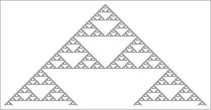
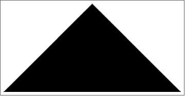
Figure 3.3: Time evolution (from the top to the bottom) starting from a single one of the ECA 18 (left) and 254 (right).

For the NDECA 18, which has $c_{7}=0$, $S_{2}=0$ and $S_{1}=2$, it is listed in Table 3.2, where the critical value $\lambda^{*}$ of the parameter $\lambda$ and the order parameter $a^{*}(\lambda)$ are reported. The MF prediction and numerical results are compared in Figure 3.4: although in both cases the phase transition is observed, the quantitative match is not very good.

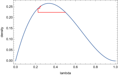
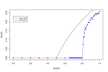
Figure 3.4: (Color online) On the left: finding the fixed point of equation (3.8) for $\lambda=0.9$ for the ECA 18. On the right: comparison between the MF prediction (solid line) for the order parameter and the numerical results (dots). Simulations have been performed starting from an initial configuration with density $1/2$, on a lattice $n=10000$ and running the simulations for the time $5000$.

We consider now the NDECA 254(11111110). ECA 254 is a simple rule having a configuration with all ones as fixed point (Wolfram’s class W1), see the right panel in Figure 3.3. For this diploid we have $c_{7}=1$, $S_{2}=3$ and $S_{1}=3$, and the associated NDECA is listed in Table 3.2, where the critical value $\lambda^{*}$ of the parameter $\lambda$ and the order parameter $a^{*}(\lambda)$ are reported. The MF prediction and numerical results are compared in Figure 3.5: the quantitative match is very good far from the critical point.

This diploid is well known in the literature and in [1, 16] is called percolation Probabilistic Cellular Automata. In [1, Example 2.4] it is proven that there exists $\lambda_{\textup{c}}\in(0,1)$ such that for $\lambda<\lambda_{\textup{c}}$ the map is ergodic and for $\lambda>\lambda_{\textup{c}}$ there are several invariant measures. In other words, for this map the paper [1] provides a rigorous proof of the existence of the phase transition. The exact value of $\lambda_{\textup{c}}$ is not known, but it is proven that it belongs to the interval $[\frac{1}{3},\frac{53}{54}]$, see [16]. A sharper result has been given in [14], where the lower bound $\lambda_{\textup{c}}>0.505$ is proven. Therefore, for the NDECA 254 the infinite volume situation is close to the simulation results discussed in [4] and illustrated in Figure 3.5. The simulations are indeed in an essentially infinite volume regime as we shall discuss in the sequel. We finally notice that the MF prediction $\lambda^{*}=1/2$ is very close to the lower bound $\lambda_{\textup{c}}>0.505$.

A third example is given by NDECA 238 (11101110). This model is called Stavskaya model and it is a particular case of the percolation PCA when we choose $Q=\{0,1\}$ instead of $Q=\{-1,0,+1\}$. Stavskaya model has a phase transition for $\lambda>\lambda_{\textup{c}}$, with $\lambda_{\textup{c}}>0.677$ (see [10]). Our MF approximation gives $\lambda^{*}=0.5$ ($c_{7}=1,\,S_{2}=3,\,S_{1}=2$).

Another example is the NDECA 102 (01100110), known as additive noise PCA and it is proven to be ergodic for all $\lambda$ (Proposition 3.5 in [11]). This result is compatible with the MF approximation that predicts the uniqueness of the invariant measure.

As a final example we consider the NDECA 17 (00010001), an odd NDECA, for which the MF predicts a unique non–null stationary measure. This model is known as directed animals PCA (see for instance Figure 7 in [11]) and it has been proven to have a unique invariant Markovian measure.

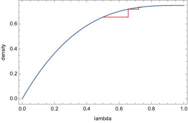
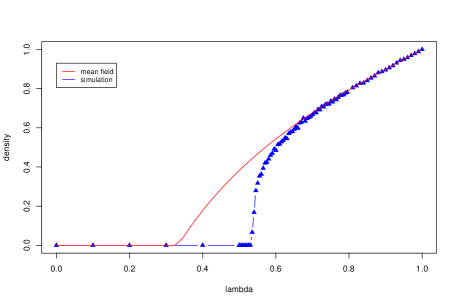
Figure 3.5: (Color online) On the left: finding the fixed point of equation (3.8) for $\lambda=0.75$ for the ECA 254. On the right: comparison between the MF prediction (solid line) for the order parameter and the numerical results (dots). Simulations have been performed starting from an initial configuration with density $1/2$, on a lattice $n=10000$ and running the simulations for the time $5000$.

4 Rigorous bounds for the critical point

The DECA defined in Section 2 with $f_{1}$ the null rule is considered here on $\mathbb{Z}$. Following [11], for some finite subset $K\subset\mathbb{Z}$, consider $y=(y_{k})_{k\in K}$. The cylinder of base $K$ defined by $y$ is the set:

$$[y]:=\left\{z\in Q^{\mathbb{Z}}:\forall k\in K,z_{k}=y_{k}\right\}$$

Thus, the probability of the cylinder of base $K$ corresponding to $y$ of the chain started in $x$, can be written as:

$$P_{x}([y]):=\prod_{i\in K}p_{i}(y_{i}|x)$$ (4.11)

with

$$p_{i}(y_{i}|x)=y_{i}\lambda f_{2}(x_{i-1},x_{i},x_{i+1})+(1-y_{i})[1-\lambda f_{2}(x_{i-1},x_{i},x_{i+1})].$$ (4.12)

Misusing the notation, we denote again by $P_{x}$ the probability associated with the infinite volume process started at $x\in X=Q^{\mathbb{Z}}$ and by $\mu^{x}_{t}(\cdot)$ the probability measure of the chain started at $x$ at time $t$.

In this framework the Dobrushin single site sufficient condition [6], stated in [10, equation (1–2)] in the case of Probabilistic Cellular Automata and extended in [10, Main Theorem], provides an instrument to prove ergodicity, and hence existence of a unique invariant measure, for NDECA. Let us introduce first the Dobrushin parameter

$$d=\sup_{a\in Q}\sum_{i\in\mathbb{Z}}\sup_{x\in Q^{\mathbb{Z}}}|p_{0}(a|x)-p_{0}(a|x^{i})|$$ (4.13)

where $x^{i}$ is the configuration such that $(x^{i})_{j}=x_{j}$ for $j\neq i$ and $(x^{i})_{i}=1-x_{i}$. By using the single–site Dobrushin Criterion [10], we have that if $d<1$ then the NDECA has a unique invariant measure.

We shall use this result, which will simply call the Dobrushin criterion, to find lower bounds to the critical value $\lambda_{\textup{c}}$ of the parameter $\lambda$. Indeed, the criterion will allow us to prove uniqueness of the invariant measure for $\lambda$ smaller than some value $\mu$, which will provide a lower bound to $\lambda_{\textup{c}}$, that is to say, $\lambda_{\textup{c}}\geq\mu$.

It is useful to note that, in our NDECA context, where we have only two symbols, the Dobrushin parameter simplifies to

$$d=\sum_{i\in\mathbb{Z}}\sup_{x\in Q^{\mathbb{Z}}}|p_{0}(1|x)-p_{0}(1|x^{i})|.$$ (4.14)

Moreover, using that $p_{0}(1|x)$ depends only on the value of the cells $i=-1,0,+1$, we can finally write

$$d=\sum_{i\in\{-1,0,+1\}}\sup_{x\in Q^{\mathbb{Z}}}|p_{0}(1|x)-p_{0}(1|x^{i})|.$$ (4.15)

Theorem 4.1.

For any choice of the ECA rule $f_{2}$,

1. for any $i\in\{-1,0,+1\}$ and $x\in Q^{3}$, $|p_{0}(1|x)-p_{0}(1|x^{i})|$ is either $0$ or $\lambda$;

2. the NDECA defined in (4.11) has a unique invariant measure for all $\lambda<1/3$.

Proof.

Item 1: from (4.12), the probability $p_{0}(1|x)$ is either $0$ or $\lambda$, hence $|p_{0}(1|x)-p_{0}(1|x^{i})|$ is either $0$ or $\lambda$. Item 2: Using item 1 and (4.15) we can then conclude that $d\leq 3\lambda$. Thus, for $\lambda<1/3$ the Dobrushin criterion ensures that the invariant measure is unique in the infinite volume case and coincides with the delta measure in $0$. ∎

Hence, by Theorem 4.1 we have the lower bound $\lambda_{\textup{c}}\geq 1/3$ for the critical value of the parameter $\lambda$. This estimate is rather poor if compared to the numerical and MF results, which predicts a value around $0.7$ for the critical point $\lambda_{\textup{c}}$. On the other hand, since the result in the Theorem 4.1 is uniform in the choice of the rule $f_{2}$ of the NDECA, one can expect that a better bound could be found if the Dobrushin criterion were applied to a particular subset of rules. In order to realize a useful classification of the NDECA we introduce the following notion: we say that the cell $i\in\{-1,0,+1\}$ is marginal for the NDECA if and only if $p_{0}(1|x)=p_{0}(1|x^{i})$ for any $x\in Q^{3}$. Note that, if $i\in\{-1,0,+1\}$ is not marginal for the NDECA then there exists $x\in Q^{3}$ such that $p_{0}(1|x)\not=p_{0}(1|x^{i})$. In other words if a NDECA has unessential cells, there exists a not empty subset of $\{-1,0,+1\}$ such that, for any configuration, the probability to set one at the origin is not affected if the value of a cell in this subset is varied, whereas there are configurations such that it changes if the value of any other cell is modified.

Theorem 4.2.

If $A\subset\{-1,0,+1\}$ is the maximal (with respect to inclusion) set of marginal cells, then $d=(3-|A|)\lambda$.

Proof.

By item 1 of Theorem 4.1 and the definition of marginal cells, we have that

$$\sup_{x\in Q^{3}}|p_{0}(1|x)-p_{0}(1|x^{i})|=\left\{\begin{array}[]{ll}0&\;\;\;\textup{if }i\in A\\ \lambda&\;\;\;\textup{otherwise}.\\ \end{array}\right.$$

The theorem then follows from (4.15). ∎

The above theorem allows a full classification of NDECA with respect to the number of marginal cells. Depending on this number the Dobrushin parameter can be exactly computed for the NDECA and hopefully the estimates of the critical point $\lambda_{\textup{c}}$ can be improved. Note that, in particular, that for a NDECA not having any marginal cells, since the maximal set of marginal set is the empty set, the Dobrushin parameter is $3\lambda$ so that in these cases the general blind bound of Theorem 4.1 is not improved. In the following sections all the possible cases will be reviewed.

4.1 Three marginal cells

This case is rather trivial. We consider the ECA mapping all configurations to the same cell value. Namely, we consider the maps 0(00000000) and 255(11111111): the first one maps all configurations to zero and the second all configurations to one. In both cases the number of marginal cells is three, so, by using Theorem 4.2, we have that $d=0$. Hence, by the Dobrushin criterion it follows that these two NDECA have a single invariant measure for any $\lambda\in(0,1)$.

4.2 Two marginal cells

All possible cases are listed in Table 4.4. Since the position of the not marginal cell can be chosen in three possible ways, we have the following six choices for the $f_{2}$ map. The not marginal cell is the left one: 240(11110000), 15(00001111). The not marginal cell is the central one: 204(11001100), 51(00110011). The not marginal cell is the right one: 170(10101010), 85(01010101). It s interesting to notice that the ECA $240$, $204$, and $170$ have a straightforward interpretation in terms of shift operators: right shift, identity, left shift. For the NDECA with rule $f_{2}$ one of the six rules listed above, since the maximal set of marginal set has cardinality equal to two, the Dobrushin parameter is $\lambda$. Hence, by the Dobrushin criterion it follows that these six NDECA have a single invariant measure for any $\lambda\in(0,1)$.

This rigorous result is coherent with simulations and the MF analysis, indeed for the six maps listed above neither simulations nor MF predict the existence of the phase transition.

not marginal	marginal	marginal	$f_{2}$	$f_{2}$
1	1	1	1	0
1	1	0
1	0	1
1	0	0
0	1	1	0	1
0	1	0
0	0	1
0	0	0

Table 4.4: Possible choices of the rule $f_{2}$ in case of two marginal cells. First column: not marginal cell. Second and third columns: marginal cells. Fourth and fifth columns possible values of $f_{2}$.

4.3 One marginal cell

Half of the possible cases are listed in Table 4.5, the remaining one can be found as described in the caption. Since the position of the marginal cell can be chosen in three possible ways, the five cases reported in the table gives rise to the following fifteen choices for the $f_{2}$ map. Marginal cell on the left: 153(10011001), 136(10001000), 187(10111011), 238(11101110), 221(11011101). Marginal cell at the center: 165(10100101), 160(10100000), 175(10101111), 250(11111010), 245(11110101). Marginal cell on the right: 195(11000011), 192(11000000), 207(11001111), 252(11111100), 243(11110011). The remaining fifteen maps can be found by those reported above by changing the zeroes with the ones so that the complement to 255 is found. Namely, we have: 102(01100110), 119(01110111), 68(01000100), 17(00010001), 34(00100010) for the marginal cell on the left, 90(01011010), 95(01011111), 80(01010000), 5(00000101), 10(00001010) for the marginal cell as central cell, 60(00111100), 63(00111111), 48(00110000), 2(00000011), 12(00001100) for the marginal cell on the right.

For the NDECA with rule $f_{2}$ one of the thirty rules listed above, since the maximal set of marginal set has cardinality equal to one, the Dobrushin parameter is $2\lambda$. Hence, by the Dobrushin criterion it follows that these thirty NDECA have a single invariant measure for any $\lambda<1/2$, which gives the lower bound $\lambda_{\textup{c}}\geq 1/2$ for the critical point.

It is worth noting that for the rules 2, 10, 34, 48, 68, 80, 136, 160, 192 neither simulations nor the MF analysis predict the phase transition. For the rules 10 and 252 the simulations do not observe the phase transition, whereas the MF approximation predict the existence of the transition with critical point $\lambda^{*}=1/2$. Finally, for the rules 60, 90, 238, and 250 both simulations and the MF analysis predict the phase transition with a MF estimate of the critical point $\lambda^{*}=1/2$.

not marginal	not marginal	marginal	$f_{2}$	$f_{2}$	$f_{2}$	$f_{2}$	$f_{2}$
1	1	1	1	1	1	1	1
1	1	0
1	0	1	0	0	0	1	1
1	0	0
0	1	1	0	0	1	1	0
0	1	0
0	0	1	1	0	1	0	1
0	0	0

Table 4.5: Possible choices of the rule $f_{2}$ in case of one marginal cell. First and second column: not marginal cells. Third column: marginal cell. Other columns: possible values of $f_{2}$. Five more cases are not listed: the values of the map $f_{2}$ are obtained by exchanging the symbols $0$ and $1$ in those reported in the table.

4.4 Examples

In this section we will look again at the examples given Section 3.4, under the perspective of the rigorous results of Section 4.

For the NDECA 18, NDECA 17 (directed animals) and NDECA 102 (noisy additive PCA) we have the Dobrushin bound: $\lambda_{\textup{c}}\geq 1/3$. However, in case of NDECA 102 (noisy additive PCA), NDECA 238 (Stavskaya model) and NDECA 254 ((percolation PCA )) we have one marginal cell (the left), so that $\lambda_{\textup{c}}>1/2$ (see Section 4.3), compatible with the known results reviewed in Section 3.4.

5 Time scales for finite volume diploids

In this section we change the perspective and examine the system in finite volume within time scales increasing with $n$. The main question is that of understanding to which extent finite volume simulations are a reasonable description of the infinite volume behaviors of diploids.

We will confine our discussion to NDECA with even $f_{2}$ rule, for which, as we have already remarked in Section 2, the measure concentrated on the zero configuration $0$ is an invariant measure at finite volume, since $p(0,x)=0$ for any $x\in X_{n}$. Moreover, since starting from any configuration the probability that the chain reaches the state $0$ is finite, we expect that any simulation, sooner or later, will be trapped in $0$. The aim of this section is precisely that of giving an estimate of the time needed by the chain to hit $0$.

We start with a a very rough heuristic argument suggesting that for $\lambda$ small enough the chain should reach the configuration $0$ in a time logarithmically increasing with the size $n$. Thus, consider a NDECA with even $f_{2}$ rule and choose the configuration $1$ as initial state:

• at the first step (time $1$) the number of $1$’s switched to $0$ is $(1-\lambda)n$, so that the number of ones at time $1$ is $n-(1-\lambda)n=\lambda n$.

• At the second step the number of $1$’s turned to $0$ will be $\lambda n(1-\lambda)$. But at this stage one has to consider that zeros can be switched to one: since the rule $f_{2}$ is even, one zero, in order to have the chance to be turned to $1$, must at least have a $1$ among its neighboring site. This, indeed, depends on the rule, but in this simple argument we consider the case which is most favorable to the $0$ to $1$ switch and assume that one single neighboring $1$ is sufficient to perform the switch according to the rule $f_{2}$. Under such assumption (exaggerating) we can estimate the number of zeros turning to one as twice the number of ones at time one times $\lambda$, namely, $2\lambda n\lambda$. Hence, at time two the number of ones will be $\lambda n-(1-\lambda)\lambda n+2n\lambda^{2}=3\lambda^{2}n$.

• Iterating the computation at time three we find $9\lambda^{3}n$ ones and at time $t$ we will find $(3\lambda)^{t}n/3$ ones. This number will be of order one at $t\sim\log(n/3)/\log(1/(3\lambda))$, meaning that for $\lambda<1/3$ we expect that in a logarithmic time the chain will converge to the zero configuration.

Thus, for $\lambda$ small the configuration $0$ is reached in a time logarithmically increasing with the size $n$. This is checked numerically in the left panel of Figure 5.6 for the $f_{2}$ map 254.

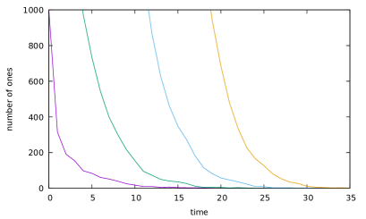
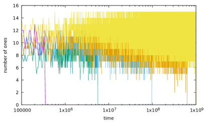
Figure 5.6: (Color online) Relaxation of NDECA with map $f_{2}$ 254 starting from the 1 configuration. On the left $\lambda=0.30$, $n=10^{3}$ (violet), $n=10^{4}$ (green), $n=10^{5}$ (blue), $n=10^{6}$ (orange); the corresponding values of the estimate $\log(n)/log(1/(3\lambda))$ for the relaxation time are $55.1$, $77.0$, $98.8$, $120.7$. On the right: the size $n$ of the lattice and the parameter $\lambda$ are chosen as follows: $n=15$ and $\lambda=0.7$ (violet), $n=10$ and $\lambda=0.82$ (green), $n=12$ and $\lambda=0.81$ (blue), $n=13$ and $\lambda=0.81$ (orange), $n=15$ and $\lambda=0.81$ (yellow); the corresponding values of the estimate $1/(1-\lambda)^{n}$ for the relaxation time are $6.9\times 10^{7}$, $2.8\times 10^{7}$, $4.5\times 10^{8}$, $2.4\times 10^{9}$, $6.6\times 10^{10}$.

The natural question, now, is about the behavior of the chain for $\lambda$ close to $1$. In the following lemma we give an upper bound for the probability of being at time $t$ in a configuration different from the stationary state $0$ and will provide us with an argument to estimate the relaxation time for $\lambda$ close to $1$.

Theorem 5.3.

Consider a NDECA with even map $f_{2}$. For any initial state $y\in X_{n}\setminus\{0\}$ we have that

$$P_{y}(\{\xi^{t}\neq 0\})\leq[1-(1-\lambda)^{n}]^{t}\leq\exp\{-t(1-\lambda)^{n}\}.$$ (5.16)

Proof.

Recall that the Markov chain is denoted by $\xi^{t}$. Since $0$ is a fixed point, for any initial state the event $\{\xi^{t}\in X_{n}\setminus\{0\}\}$ is a subset of the event $\{\xi^{t-1}\in X_{n}\setminus\{0\}\}$. Thus, given the initial state $y$, we have

$$P_{y}(\{\xi^{t}\neq 0\})=P_{y}(\{\xi^{t}\neq 0\}\cap\{\xi^{t-1}\neq 0\})=\sum_{x\neq 0}P_{y}(\{\xi^{t}\neq 0\}\cap\{\xi^{t-1}=x\})$$

and using the Markov property we get

$$P_{y}(\{\xi^{t}\neq 0\})=\sum_{x\neq 0}P_{y}(\{\xi^{t}\neq 0\}|\{\xi^{t-1}=x\})P_{y}(\{\xi^{t-1}=x\})$$

which yields the recursive bound

$$\begin{array}[]{rcl}P_{y}(\{\xi^{t}\neq 0\})&\leq&{\displaystyle\sup_{x\neq 0}P_{y}(\{\xi^{t}\neq 0\}|\{\xi^{t-1}=x\})\sum_{x\neq 0}P_{y}(\{\xi^{t-1}=x\})}\\ &=&{\displaystyle\sup_{x\neq 0}P_{y}(\{\xi^{t}\neq 0\}|\{\xi^{t-1}=x\})P_{y}(\{\xi^{t-1}\neq 0\})\;\;.}\end{array}$$

Moreover, we note that

$$\begin{array}[]{rcl}{\displaystyle\sup_{x\neq 0}P_{y}(\{\xi^{t}\neq 0\}|\{\xi^{t-1}=x\})}&=&{\displaystyle\sup_{x\neq 0}[1-P_{y}(\{\xi^{t}=0\}|\{\xi^{t-1}=x\})]}\\ &=&{\displaystyle 1-\inf_{x\neq 0}P_{y}(\{\xi^{t}=0\}|\{\xi^{t-1}=x\}).}\end{array}$$

Since to put $0$ in a cell has a probability cost at least $1-\lambda$, we have that

$$\inf_{x\neq 0}P_{y}(\{\xi^{t}=0\}|\{\xi^{t-1}=x\})\geq(1-\lambda)^{n}\;\;.$$

Collecting all the bounds and iterating with respect to $t$ we have that

$$\begin{array}[]{rcl}P_{y}(\{\xi^{t}\neq 0\})&\leq&{\displaystyle[1-(1-\lambda)^{n}]P_{y}(\{\xi^{t-1}\neq 0\})}\\ &\leq&{\displaystyle[1-(1-\lambda)^{n}]^{t-1}P_{y}(\{\xi^{1}\neq 0\})\leq[1-(1-\lambda)^{n}]^{t}.}\end{array}$$

The second bound is immediate. ∎

As we noticed before for $\lambda$ small a time $t(n)$ diverging logarithmically with $n$ seems to be sufficient for the finite volume diploid to approach the $0$ state, in the sense that $P_{y}(\{\xi^{t(n)}\neq 0\})$ tends to zero as $n\to\infty$. The above theorem, for any $\lambda\in(0,1)$, proves a weaker, but rigorous, statement: a time $t(n)$ diverging exponentially with $n$ is sufficient for the finite volume diploid to relax to the $0$ state in the sense specified above. Indeed, if $t(n)=\alpha^{n}$, with $\alpha\geq 1/(1-\lambda)$, then from Theorem 5.3 it follows that

$$P_{y}(\{\xi^{t(n)}\neq 0\})\leq e^{-[\alpha(1-\lambda)]^{n}}\to 0$$

in the limit $n\to\infty$. The Theorem 5.3 is useless for times $t(n)$ smaller than $(1-\lambda)^{n}$, namely, such that $t(n)(1-\lambda)^{n}\to 0$. Indeed, in such a case the r.h.s. of (5.16) tends to $1$ and the bound is trivial.

This behavior, which shares some common feature with metastable states, is checked numerically in the right panel of Figure 5.6 for the NDECA with $f_{2}$ map number 254. We had to use ridiculously small lattices, i.e., $n=10,12,13,15$, due to the exponential dependence of the relaxation time on $n$. In the picture on the horizontal axis we report the time on a logarithmic scale and on the vertical axis we report the number of cells with value one. Notice that in a time of order $10^{9}$ all the diploid ECA except the yellow one relax to the stationary state $0$.

Finally, we come back to the original question about the ability of the simulation to catch the infinite volume behavior of the NDECA. As it is absolutely reasonable, from the Theorem 5.3 it follows immediately that for a fixed $n$ the diploid converges to the stationary state $0$ with probability one in the limit $t\to\infty$. How is this result compatible with the numerical studies presented in Section 2? Indeed, those simulations are obviously performed at finite volume, nevertheless the system is found in a stationary state with density different from zero. The key is the choice of the time–scales considered in the simulations and the size $n$ of the chain: in the simulations $n=10^{4}$ and $t=5\cdot 10^{3}$, the bound (5.16) is thus irrelevant, indeed, $[1-(1-\lambda)^{n}]^{t}=[1-0.15^{10^{4}}]^{5\cdot 10^{3}}\cong 1$. It is reasonable to suppose that for that choice of the parameters, the system is essentially in the infinite volume regime, where the probability of flipping to zero at the same time a large number of cells is negligible.

The problem of the relaxation time has been treated at a high level of generality, namely, we considered any NDECA with $f_{2}$ an even map. In this perspective it is not possible to be more precise about the behavior of the relaxation time with respect to the volume $n$ of the system. On the other hand, considering particular NDECA one can prove more precise statements, as we discuss in the following subsections.

5.1 The case of the identity: logarithmic behavior of the relaxation time

Consider the NDECA with the map $f_{2}$ being the identity, namely, the rule 204(11001100): as mentioned in Section 2 this rule associates to any configuration the state of the cell at the center of the neighborhood, namely, the cell that one is going to update. Cells are thus updated independently one from each other but not on the past. The chain can be described as a collection of $n$ single cell Markov chains evolving with the transition matrix

$$q(0,0)=1,\;q(0,1)=0,\;q(1,0)=1-\lambda,\;q(1,1)=\lambda,$$

for any cell $i\in\mathbb{L}_{n}$. The stationary measure is product and the single cell stationary measure is concentrated on $0$, namely, $\pi_{i}(0)=1$ and $\pi_{i}(1)=0$. Moreover, for a single cell started at $1$, the probability that its state is $0$ at time $t$ is equal to $1-\lambda^{t}$, namely, $1$ minus the probability that from time $1$ to time $t$ it has always been sampled the rule $f_{2}$. Hence, if we look at the whole chain, we have that $\mu_{t}^{1}(0)=(1-\lambda^{t})^{n}$. Now, suppose to compute this probability on a time scale diverging logarithmically with $n$, namely, take $t(n)=\alpha\log n$ for some $\alpha$ such that $\alpha>-1/\log\lambda$:

$$\mu_{t}^{1}(0)=(1-\lambda^{t})^{n}\approx e^{-n\lambda^{\alpha\log n}}=e^{-\exp\{(1+\alpha\log\lambda)\log n\}}\to 0$$

in the limit $n\to\infty$. Thus, for any $\lambda\in(0,1)$, the NDECA under consideration will converge in probability to $0$, namely in this case the relaxation time is logarithmically large in $n$ (see Figure 5.7).

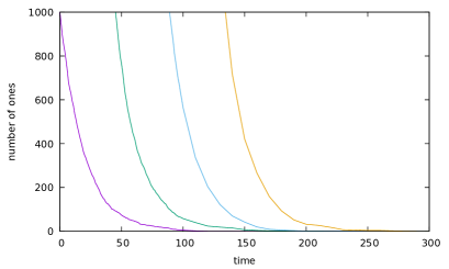
Figure 5.7: (Color online) Relaxation of NDECA with map $f_{2}$ 204 (identity) starting form the 1 configuration with $\lambda=0.95$, $n=10^{3}$ (violet), $n=10^{4}$ (green), $n=10^{5}$ (blue), $n=10^{6}$ (orange); the corresponding estimates $(-1/\log\lambda)\log n$ for the relaxation time are $134.7$, $179.5$, $224.4$, $269.3$.

5.2 The case of the percolation PCA: exponential behavior of the relaxation time

We consider, here, the NDECA with map 254 as map $f_{2}$, which, as discussed above, is an example of percolation PCA. In Figure 5.6 we have shown that for $\lambda$ small the relaxation time diverges logarithmically with $n$, whereas for $\lambda$ large this divergence is exponential. We have supported these conclusions with some analytical argument.

Indeed, for the percolation PCA this result is proven rigorously in [14, Theorem 2.1]. In this paper the author proves for the critical point the bound $\lambda_{\textup{c}}\geq 0.505$, see the table in the Appendix therein. Moreover the Theorem 2.1 which provides an estimate for the average relaxation time, can be restated as follows.

Theorem 5.4.

For the NDECA with map $f_{2}$ the ECA 254, let $\tau$ be the first hitting time to the state $0$ starting from the state $1$, then there exists $n_{0}\in\mathbb{N}$ and some positive constants $K_{1}$, $K_{2}$, $K_{3}$, $K_{4}$, $c_{1}$, $c_{2}$, $c_{3}$, and $c_{4}$ (dependent on $\lambda$) such that for all $n>n_{0}$

• if $\lambda<\lambda_{\textup{c}}$ then $K_{1}\log(c_{1}n)\leq\mathbb{E}_{1}[\tau]\leq K_{2}\log(c_{2}n)$;

• if $\lambda>\lambda_{\textup{c}}$ then $K_{3}\,\textup{exp}(c_{3}n)\leq\mathbb{E}_{1}[\tau]\leq K_{4}\,\textup{exp}(c_{4}n)$;

where we denote by $\mathbb{E}_{1}$ the mean on the trajectories of the Markov chain started at $1$.

6 Conclusions

We have studied the possibility for diploid Elementary Cellular Automata (DECA) to exhibit phase transitions. In particular we have analyzed the case in which one of the two ECA mixed to obtain the DECA is the null rule. In such case we have called NDECA the DECA so obtained.

The problem has been approached via a MF approximation and through the use of the rigorous Dobrushin Criterion. The two methods have allowed two different classifications of NDECA. The two approaches give coherent results and, to some extent, explain and justify some of the numerical results discussed in [4].

As we have often repeated, the point of view followed in this paper, and mainly borrowed from [4], allow a unified approach to many different PCA which has been studied in the Probability and Statistical Mechanics literature putting them in a different light. In some dedicated sections, for the PCA that we have been able to spot in the past literature, we have compared our results with some rigorous statements already present in the literature.

Acknowledgements

The authors thank R. Fernandez and N. Fatès for very useful discussions. ENMC expresses his thanks to the Mathematics Department of the Utrecht University for kind hospitality and STAR for financial support. The research of Francesca R. Nardi was partially supported by the NWO Gravitation Grant 024.002.003–NETWORKS and by the PRIN Grant 20155PAWZB Large Scale Random Structures.

References

- [1] A. Busic, J. Mairesse, I. Marcovici, Probabilistic cellular automata, invariant measures, and perfect sampling, Adv. in Appl. Probab. 45, 960-1980 (2013).
- [2] P. Chassaing, J. Mairesse, A non-ergodic probabilistic cellular automata with a unique invariant measure, Stochastic Process. Appl. 125, 2472–2487 (2010).
- [3] E. N. M. Cirillo, F. R. Nardi, C. Spitoni, Basic Ideas to Approach Metastability in Probabilistic Cellular Automata in Probabilistic Cellular Automata: theory, applications and future perspectives, Springer (2016).
- [4] N. Fatés, Diploid Celluar automata: First Experiments on the Random mixtures of Two Elementary Rules, Lectures Notes in Computer Science 10248, 97–108, 2017.
- [5] D. Dhar, Exact solution of a directed-site animals-enumeration problem in three dimensions, Phys. Rev. Lett. 51, 853-856 (1983).
- [6] R.L. Dobrushin, Markov Processes with a large number of locally interacting components: Existence of a limit process and its ergodicity. Problems Inform. Transmission 7, 149–164 (1971).
- [7] H. A. Gutowitz, J. D. Victor, Local Structure Theory in More than One Dimension, Complex Systems, 1, 57–68 (1987).
- [8] B. Jahnel, C. Kulske, A class of non-ergodic probabilistic cellular automata with unique invariant measure and quasi-periodic orbit, Stoch. Process. Appl. 125, 2427-2450 (2015).
- [9] P. Y. Louis, F. R. Nardi, Probabilistic Cellular Automata: theory, applications and future perspectives, Springer (2016).
- [10] C. Maes, S. Shlosman, Ergodicity of Probabilistic Cellular automata: A Constructive Criterion. Communication in Mathematical Physics 135, 233-251 (1991).
- [11] J. Mairesse, I. Marcovici, Around probabilistic cellular automata Theoretical Computer Science 559, 42-72 (2014)
- [12] H. V. McIntosh, Wolfram’s Class IV and a Good Life, Physica D 45, 105–121 (1990).
- [13] J. R. G. Mendonca, Monte Carlo investigation of the critical behavior of Stavskaya’s probabilistic cellular automaton Phys. Rev. E 83, 42-72 (2011)
- [14] L. Taggi, Critical Probabilities and Convergence Time of Percolation Probbilistic Cellular Automata, Journal of Statistical Physics 159, 853–892, 2015.
- [15] A. Toom, N. Vasilyev, O. Stavskaya, L. Mityushin, G. Kurdyumov, S. Pirogov, Discrete local Markov systems, in: R. Dobrushin, V. Kryukov, A. Toom (Eds.), Stochastic Cellular Systems: Ergodicity, Memory, Morphogenesis, Manchester University Press (1990).
- [16] A. Toom, Contours, convex sets and cellular automata IMPA mathematical publications (2004)
- [17] S. Wolfram, Statistical mechanics of cellular automata, Rev. Mod. Phys. 35, 601–644 (1983)
- [18] S. Wolfram, Computation theory of cellular automata, Comm. Math. Phys. 96, 15–57 (1984)