Jovian Auroral Radio Source Occultation Modelling and Application to the JUICE Science Mission Planning

Abstract

Occultations of the Jovian low frequency radio emissions by the Galilean moons have been observed by the PWS instrument of the Galileo spacecraft. We show that the ExPRES (Exoplanetary and Planetary Radio Emission Simulator) code accurately models the temporal occurrence of the occultations in the whole spectral range observed by Galileo/PWS. This validates of the ExPRES code. he method can be applied for preparing the JUICE moon flyby science operation planning.

[1] organization=LESIA, Observatoire de Paris, CNRS, PSL Research University, city=Meudon, country=France

[2] organization=School of Cosmic Physics, DIAS Dunsink Observatory, Dublin Institute for Advanced Studies, city=Dublin, country=Ireland

[3] organization=Aurora B.V., for European Space Agency, ESAC, city=Madrid, country=Spain

[4] organization=Rhea Group, for European Space Agency, ESAC, city=Madrid, country=Spain

1 Introduction

The magnetosphere of Jupiter produces low frequency radio emissions regions, along the active magnetic field lines connected to the Jovian auroral oval as well as to the Galilean moon auroral magnetic footprints. The Jovian radio emissions are intense and non-thermal radio frequency phenomena, spanning from a few kHz to about 40 MHz are produced through the Cyclotron Maser Instability (CMI), which converts the local plasma free-energy into electromagnetic radiation . They are used as a proxy for the Jovian magnetospheric activity. They discovered by Burke and Franklin (1955) and have been since studied with ground observatories (e.g., Nançay Array, Lamy et al., 2017) and space-borne instruments (with, e.g., the Voyager, Galileo, Cassini and Juno space missions).

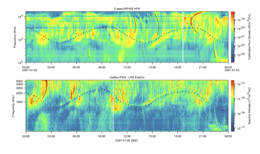
Figure 1: Calibrated Cassini/RPWS/HFR (Zarka et al., 2004; Cecconi and Zarka, 2019) (top) and GLL/PWS (see Section 2.1) (bottom) radio electric power spectral densities during 24 hours close to the Cassini flyby of Jupiter. Significant features have been highlighted: a few radio emission “arcs” are traced in plain line; Type III Solar radio bursts are traced in dashed line; and the attenuation lanes are traced in dotted line.

Observations from the Cassini Radio and Plasma Science (RPWS, Gurnett et al., 2004) and Galileo Plasma Science (PWS, Gurnett et al., 1992) experiments showed that the Jovian radio emission events are observed quasi-permanently along the spacecraft orbit. Figure 1 shows 24 hours of simultaneously observed spectral flux densities by the Cassini/RPWS and Galileo/PWS instruments, when Cassini was close to its flyby of Jupiter. Both panels of this figure display many arc-shaped radio events (a few of them are highlighted with a thin plain black line), with a few small time-frequency regions with quiet (background level) conditions. Radio arcs can be classified with orientation of their curvature: “vertex-early” and “vertex-late” arcs corresponds to opening “(” or closing “)” parenthesis shapes. The arc shape of Jovian radio emission is well explained by the CMI mechanism at the radio source, coupled with the shape of the magnetic field lines, and the rotation of Jupiter with respect of the observer, as described in Fig. 1 of Louis et al. (2019a). This figure also two other features of the observed radio spectrum around Jupiter: Type Solar radio bursts are also observed depending on the solar activity (three events are highlighted with a thin dashed black line); and the so-called “attenuation lanes” (Gurnett et al., 1998) resulting from the propagation of hectometric waves through the Io plasma torus (Menietti et al., 2003). The attenuation lanes are observed as a narrow-band attenuation feature modulated at the planetary rotation period. The attenuation is also accompanied or replaced with an intensification of the signal, to caustic optical phenomena.

Although not covering the full spectral range of the Jovian radio emissions, Galileo/PWS radio observations during its many orbits in the Jovian system. This data (Gurnett et al., 1997) shows quasi continuous emission from a few 100 kHz up to 5.6 MHz, the upper spectral limit of PWS. During the Galilean moon flybys, Galileo/PWS observed full occultations of the Jovian radio emissions (Kurth et al., 1997).

The ESA JUICE (JUpiter ICy moon Explorer, Witasse, 2019) will explore the Jupiter system and its magnetosphere. The study of the Jovian magnetosphere can strongly benefit from remote observations and modelling tools (Cecconi, 2019). Two instruments of the JUICE scientific payload in the low frequency radio range (below 50 MHz): the Radio and Plasma Waves Instrument (RPWI, Wahlund, 2013) has a receiver dedicated to the study of Jovian radio emissions; and the Radar for Icy Moon Exploration (RIME) experiment (Bruzzone et al., 2013) with a central frequency at 9 MHz, which lies within the Jovian radio emission spectral range. The Jovian radio emission may interfere with RIME active radar mode (Cecconi et al., 2012), but can be also used in a passive radar experiment mode during icy moon flybys (Romero-Wolf et al., 2015; Schroeder et al., 2016; Kumamoto et al., 2017).

The ExPRES code (Exoplanetary and Planetary Radio Emissions Simulator, Louis et al., 2019a) simulates for a given observer the geometrical visibility of radio emissions of a magnetised body. This visibility depends in particular of between the magnetic field vector at the source and the emitted wave vector, which is computed self-consistently in the frame of the CMI theory. The anisotropic shape of the radio source and their geometrical observability conditions are well described in Fig. 1 (panels c, d and e) of Louis et al. (2019a). This computation is iterated at each time/frequency step and for each source. The produced time-frequency map (or dynamic spectrum) can then directly be compared to observations.

In this study, we the Jovian radio emission occultations during (past) Galileo and (planned) JUICE Galilean moon flybys, using the ExPRES code.

2 Data Sets

Several sets of data have been used in this study and are presented in this section. For the Galileo spacecraft flybys, we compare the actual observed radio low frequency radio occultations predicted by the ExPRES code, using the actual flyby geometry (spacecraft and moon trajectory in a Jovian reference frame). The JUICE spacecraft study only includes modelled

2.1 Galileo PWS Observations

All Galilean moon flyby of Galileo with PWS data have been modelled and analysed. The Galileo PWS (hereafter referred to as GLL/PWS) data have been retrieved from University of Iowa das2 server interface (Piker et al., 2019), using the das2py python module. We have used the GLL/PWS LRS 152-channel calibratedelectric collection from that das2 server. The data are radio-electric power spectral densities provided in units of V²/m²/Hz. This dataset doesn’t include the instrument’s antenna gain calibration, but this has no consequence on this study. The data set has a native time resolution of 18.67 seconds. These data are also available in the full resolution GLL/PWS dataset (GO-J-PWS-2-REDR-LPW-SA-FULL-V1.0, Gurnett et al., 1997), at NASA PDS (Planetary Data System) PPI (Planetary Plasma Interaction) node.

2.2 Moons and Spacecraft Trajectory Data

The moons and spacecraft trajectory data are computed using SPICE kernels (Acton, 1996). In this study, the ephemeris data have been retrieved using the NASA-JPL (Jet Propulsion Laboratory of the National Aeronautics and Space Administration) instance of WebGeoCalc (Acton et al., 2018) for Galileo spacecraft and Jovian moons, and another WebGeoCalc instance at ESA-ESAC (European Space Astronomy Centre of the European Space Agency) for the JUICE spacecraft. The JUICE spacecraft SPICE kernels (ESA SPICE Service, 2020) contains all the studied orbital scenarii, as described in the JUICE CReMA (Consolidated Report on Mission Analysis) documents. In this study, the selected JUICE trajectory scenario is The ephemeris of all bodies have been retrieved in the IAU_JUPITER reference frame, also referred to as “IAU Jupiter System III (1965)”. In the WebGeoCalc interface, we use the “planetocentric” representation for coordinate retrieval, in which the longitude is oriented Eastward.

For each flyby, two ephemeris data files are retrieved, using the ‘State Vector’ WebGeoCalc capability: (a) the location of the moon and (b) that of the spacecraft, both in the IAU_JUPITER frame, as seen from the center of Jupiter, with a time interval of a few hours (2 to 4 hours, depending on the spacecraft velocity relative to the moon) on the closest approach epoch of the flyby, and a time sampling step of one minute. We do not correct for light time propagation. The resulting uncertainty in ephemeris data timing is of the order of 1 second, which is much below time resolution of the data and the simulations.

3 Jovian Radio Emissions Occultations

As shown by Kurth et al. (1997), the Jovian hectometric radio emissions are occulted by Ganymede during G01 flyby (Ganymede flyby during the first orbit around Jupiter) of the Galileo spacecraft, on June 27th 1996. Figure 1 of Kurth et al. (1997) shows the GLL/PWS spectrogram during G01 flyby (also displayed on the bottom-left panel of Figure 2). The full occultation is observed between 05:50 and 06:20 SCET. The occultation spectral ingress and egress profiles imply that the observed radio sources at higher frequencies (located close to Jupiter) are occulted earlier and reappears later than the lower frequency ones, which are located out from Jupiter. Possible occultation of the Jovian radio emissions have been also reported during the first Io flyby of Galileo (Louarn et al., 1997).

Table 1 shows our assessment of all targeted Galilean moon flybys by the Galileo spacecraft. Appendix D provides access to the full material used to conduct this study, with figures corresponding to each flyby. In this paper, we have selected one flyby of each Galilean moon, where the radio emission occultation was clearly observed (see the grey rows in Table 1). Figure 2 shows GLL/PWS observations for each of the selected flybys, i.e., from left to right and top to bottom: Io (I24), Europa (E12), Ganymede (G01) and Callisto (C30) flybys.

Orbit	Moon	Moon	Data Availability		Occultation
Name	Name	Closest Approach	GLL/PWS	SPICE	Assessment
I00	Io	1995-12-07 17:45:58	yes	yes	(?)
G01	Ganymede	1996-06-27 06:29:07	yes	yes	yes
G02	Ganymede	1996-09-06 18:59:34	yes	yes	(?)
C03	Callisto	1996-11-04 13:34:28	yes	yes	(?)
E04	Europa	1996-12-19 06:52:58	yes	yes	no
E06	Europa	1997-02-20 17:06:10	yes	yes	(?)
G07	Ganymede	1997-04-05 07:09:58	yes	yes	(?)
G08	Ganymede	1997-05-07 15:56:10	yes	yes	yes
C09	Callisto	1997-06-25 13:47:50	yes	yes	(?)
C10	Callisto	1997-09-17 00:18:55	yes	yes	no
E11	Europa	1997-11-06 20:31:44	yes	yes	no
E12	Europa	1997-12-16 12:03:20	yes	yes	yes
E14	Europa	1998-03-29 13:21:05	yes	yes	(?)
E15	Europa	1998-05-31 21:12:57	yes	no	yes
E16	Europa	1998-07-21 05:03:45	yes	yes	(?)
E17	Europa	1998-09-26 03:54:20	yes	yes	(?)
E18	Europa	1998-11-22 11:38:26	no	yes	—
E19	Europa	1999-02-01 02:19:50	yes	yes	(?)
C20	Callisto	1999-05-05 13:56:18	yes	yes	no
C21	Callisto	1999-06-30 07:46:50	yes	yes	no
C22	Callisto	1999-08-14 08:30:52	yes	yes	yes
C23	Callisto	1999-09-16 17:27:02	yes	yes	yes
I24	Io	1999-10-11 04:33:03	yes	yes	yes
I25	Io	1999-11-26 03:59:15	yes	yes	(?)
E26	Europa	2000-01-03 17:59:56	yes	yes	no
I27	Io	2000-02-22 13:46:36	yes	yes	yes
G28	Ganymede	2000-05-20 10:10:18	yes	yes	no
G29	Ganymede	2000-12-28 08:25:27	yes	yes	no
C30	Callisto	2001-05-25 11:23:58	yes	yes	yes
I31	Io	2001-08-06 04:59:21	yes	yes	no
I32	Io	2001-10-16 01:23:21	yes	yes	(?)
I33	Io	2002-01-17 14:08:23	yes	yes	(?)

Table 1: List of all targeted Galilean moon flybys with PWS/Electric-Survey data. The data from all flybys (except E18) are available through the University of Iowa das2 server end-point. The spacecraft ephemeris data is available for all flybys except E15. The occultation assessment indicates if the occultation is observed (yes or no) or unsure (?). The grey lines correspond to the flybys shown in Figure 2 and described in in this study. Table adapted from Table 1 (Orbital Facts) of the CATALOG/GO_MISSION.CAT label file available from Gurnett et al. (1997)

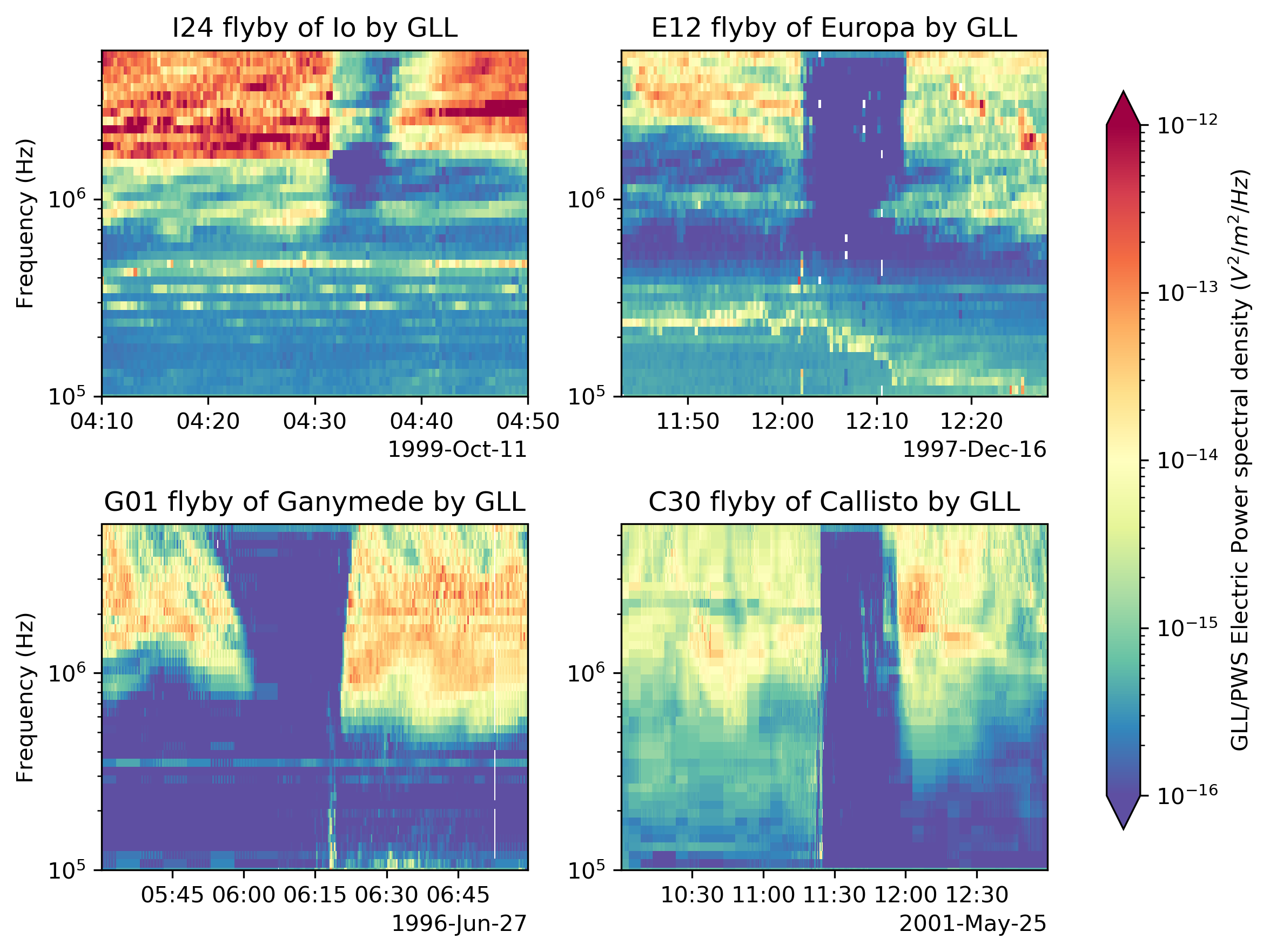
Figure 2: Jovian radio emission occultations by Io (upper left), Europa (upper right), Ganymede (lower left) and Callisto (lower right), as seen by GLL/PWS. The figures are showing radio electric power spectral densities in V²/m²/Hz.

3.1 Radio Emission

We model the location of the Jovian auroral radio sources visible at Galileo’s location using ExPRES (version 1.1.0, Louis et al., 2020)). Our simulation runs are configured as follows: (a) we use the JRM09 magnetic field model (Connerney et al., 2018) together with the Connerney et al. (1981) current sheet model; (b) the sources are set every 1^∘ in longitude along active magnetic field lines of $\textrm{M-shell}=30$ (M-shell being the measure of the magnetic apex, i.e., the distance in Jovian radii ($R_{J}$), of the magnetic field line at the magnetic equator), corresponding to the main auroral oval (Grodent, 2015); (c) the unstable electron temperature is set to 5 keV (Louarn et al., 2017); and (d) the location of the visible radio sources is with a temporal step of one minute. These parameters are fixed for all simulation runs used in this study. We also included Io-induced radio emissions in the simulation runs, with the same unstable electron distribution temperature (5 keV). The ExPRES configuration available, as described in appendix D.

When the observer is located near the magnetic equator, the radio source beaming pattern implies that the visible radio are split into four cluster locations, called A, B, C and D, corresponding respectively to the North-Eastern, North-Western, South-Eastern and South-Western quadrant around Jupiter as seen from the observer (see, e.g., Fig. 2 of Marques et al., 2017, for a definition).

The simulation runs have been computed using the OPUS (Observatoire de Paris UWS Server, Servillat et al., 2021a) instance operated by PADC for the MASER (Measurement, Analysis and Simulation of Emissions in the Radio range) project (Cecconi et al., 2020). OPUS is a framework running the Universal Worker Service (UWS) protocol (Harrison and Rixon, 2016). The ExPRES code is available for run-on-demand from this interface.

3.2 Occultation

The occultation is computed using a simple geometric derivation of the intercept distance between the center of the Galilean moon and the straight lines passing by each visible modelled radio source and the observer. Any source with an intercept distance shorter than one moon radius is occulted, assuming a spherical moon, as sketched on Figure 3.

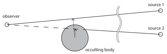
Figure 3: Simple geometric occultation scheme used in this study. The interception distance (dotted segment) is computed as the distance between the center of the occulting body and the line of sight between the observer and the source. In this case the source 1 is not occulted, while source 2 is.

3.3 Occultation timing uncertainty

Figure 4: Simple flyby geometry used to evaluate the occultation timing uncertainty. The observer is noted “S/C”. $\vec{V}$ is the relative velocity of the observed moon with respect to the observer. $d$ is the distance of the observer to the moon. $\delta\theta$ is the angular uncertainty of the radio source location.

4 Observations

All Galileo flybys have been analysed and modelled using ExPRES. In this section, we present the detailed modelling results corresponding to the highlighted rows of Table 1. Figures 5, 6, 7 and 9 present the results for these four flybys. The flybys are presented in order to show the simpler to the more complex cases. The GLL/PWS data (same data as in Figure 2) are plotted together with the simulations of observable auroral radio emissions (described in Section 3.1) separated into the four source types A, B, C and D (from white to black, respectively). The comparison of observations and modelled data shows that the simulations reproduce the Jovian radio occultation during the four flybys presented in Figure 2.

D describes the supplementary material available for all flybys (Cecconi et al., 2021), which contains all the material used to conduct this study. For each Galileo flyby, we provide: (a) a figure showing the GLL/PWS data and the observable radio sources by ExPRES, and (b) movies showing a subset of Jovian radio sources (a selected sub-set of frequencies), as seen from Galileo (‘pov’ movies), or from the top of the Jovian system (‘top’ movies).

4.1 Callisto C30 flyby

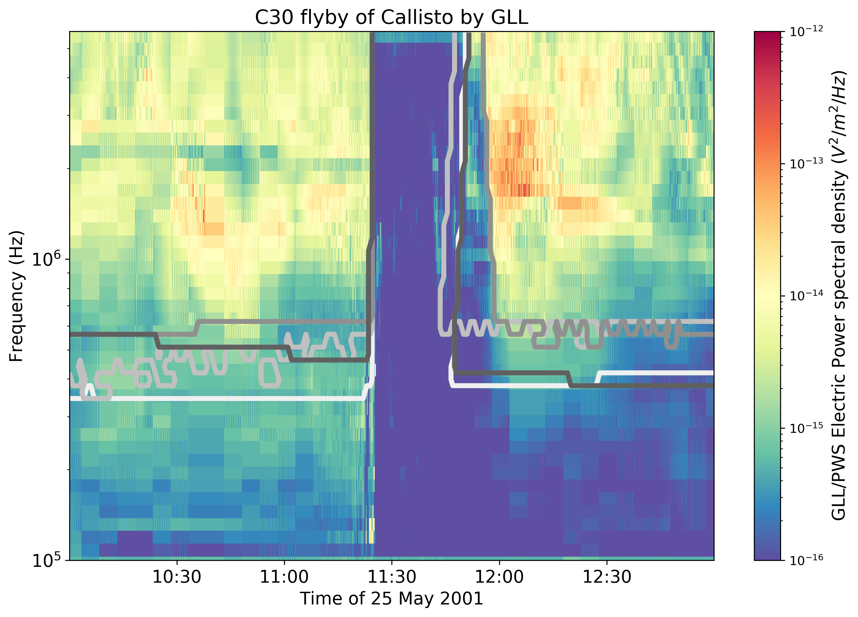
Figure 5: Superimposed GLL/PWS data and ExPRES simulations during Jovian radio emission occultations by Callisto (flyby C30). The four types of emission (A, B, C, D) are separated (from white to dark grey, resp.)

The occultation occurring during the C30 flyby of Callisto is displayed in Figure 5. The ingress occultation time is very well reproduced (within one minute accuracy). All sources are occulted simultaneously, with radio emissions intensity dropping instantly, at $\sim$11:25 SCET. At egress, we observe first a faint rise of the emission intensity from $\sim$11:50 to $\sim$12:00, and then a sudden return to maximum intensity at $\sim$12:00. This egress phase can be visualised in the supplementary material available for this flyby: https://doi.org/10.25935/8ZFF-NX36#C30. The frames between 11:44 to 11:59 of the ‘pov’ movie clearly shows the various sources reappearing one after the other: first, the B sources, then the A and D sources simultaneously and finally the C sources. The predicted reappearance of C sources perfectly coincides with the observed full egress phase. This leads to two observations: (i) the main radio contribution is that of the C sources at the time of observation, and (ii) the radio sources are occulted by the moon’s surface (or very close to it).

The low-frequency cut-off is not perfectly simulated (especially on the ingress side), with a of about $200$ kHz

An attenuation feature is observed starting at $\sim$2.5 MHz, and decreasing to $\sim$2 MHz at ingress. This corresponds to the attenuation lanes described in the introduction section. In addition, during the full occultation period of time, unexpected faint and sporadic signals are observed between $\sim$800 kHz and $\sim$2 MHz.

4.2 Europa E12 flyby

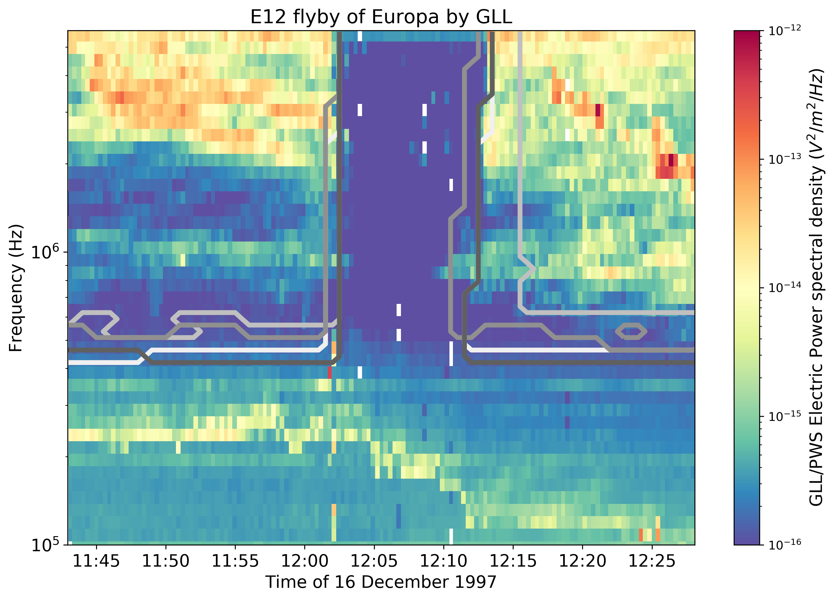
Figure 6: Superimposed GLL/PWS data and ExPRES simulations during Jovian radio emission occultations by Europa (flyby E12). The four types of emission (A, B, C, D) are separated (from white to dark grey, resp.)

The E12 flyby (Fig. 6) is similar to C30 Callisto’s flyby case, where all sources are occulted simultaneously at ingress. Faint and sporadic radio signatures are observed during the full occultation phase (as in the case of C30). At egress, the simulation well reproduces the end of the occultation, except in the $\simeq$ [$800$-$1000$] kHz frequency range where we observed emission during the modelled occultation. https://doi.org/10.25935/8zff-nx36#E12

The attenuation lane feature is observed at and below $\sim$2 MHz before ingress, with a corresponding feature after egress, up to $\sim$12:20. At about $\sim$1 MHz, an intensification is also observed, before ingress and after egress (corresponding to the aforementioned prediction mismatch), and is probably linked to the attenuation lanes.

The spectral line observed between $\sim$250 kHz (at the beginning of the interval) and $\sim$100 kHz (at the end) corresponds to the local plasma upper-hybrid frequency line

4.3 Ganymede G01 flyby

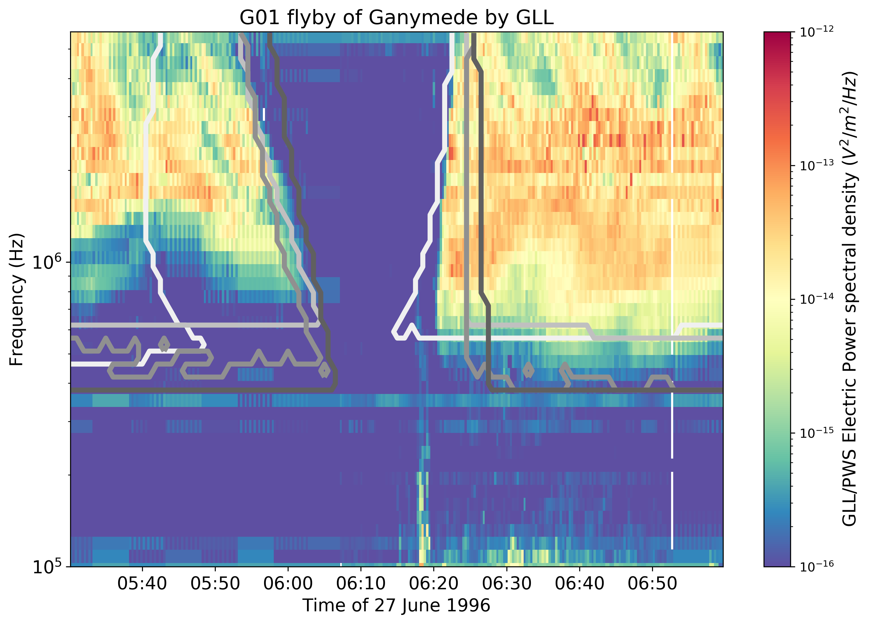
Figure 7: Superimposed Galileo PWS data and ExPRES simulations during Jovian radio emission occultations by Ganymede (flyby G01). The four types of emission (A, B, C, D) are separated (from white to dark grey, resp.)

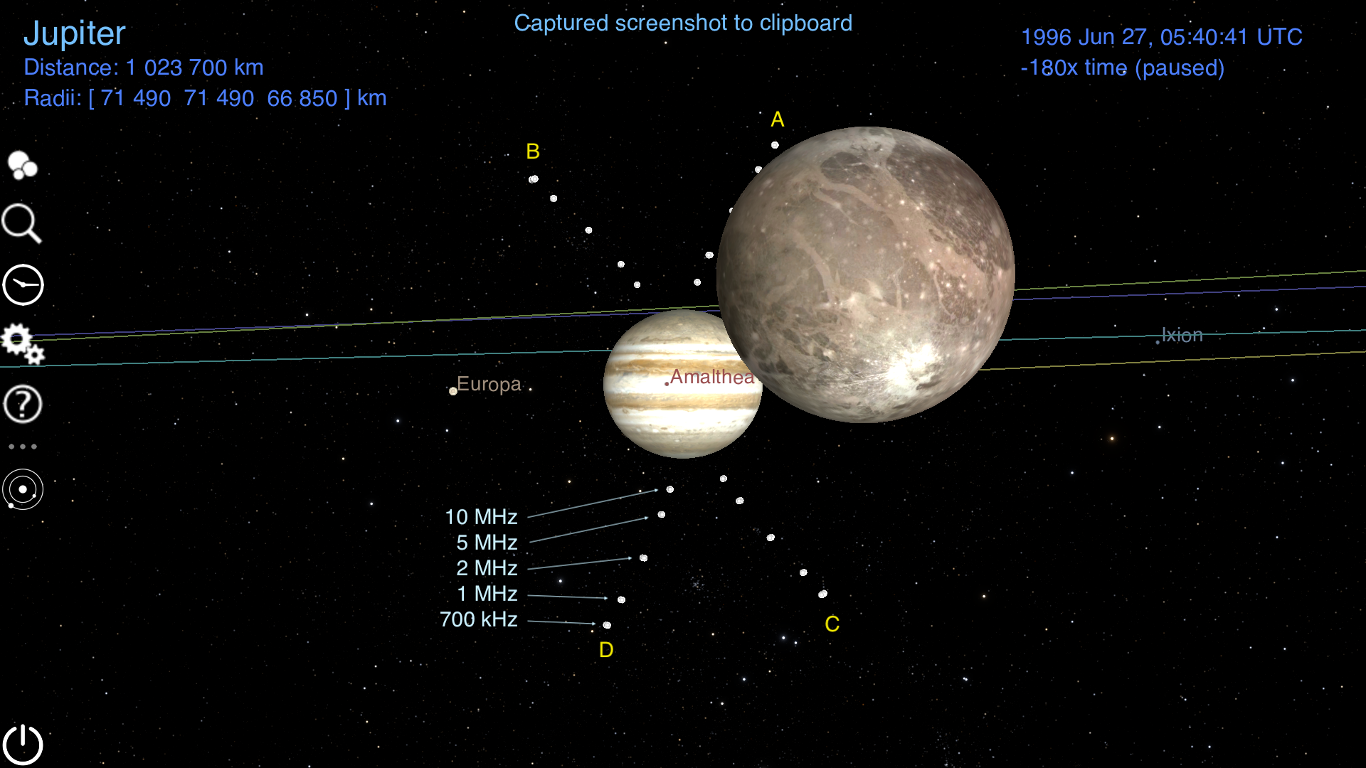
Figure 8: G01 Flyby visualised in the Cosmographia tool. The scene is set with an observer on the Galileo spacecraft, pointing to Jupiter. Ganymede is in the field of view. The ExPRES-modelled visible radio sources are also shown, at 700 kHz, 1 MHz, 2 MHz, 5 MHz and 10 MHz. The radio sources are naturally grouped in four sets (named A, B, C and D). A the time of the snapshot (1996-06-27T05:40:41 SCET), at 2 MHz in the A-group.

Figure 7 displays the occultation modelling of the Jovian radio emissions during the G01 flyby of Ganymede. At ingress, unlike the previous two cases, all sources are not occulted simultaneously. First the A sources are occulted, then the B, C and D sources, with the beginning of the full occultation. Before observed egress, a broadband noise burst at $\sim$06:18, going up to $\sim$800 kHz. This has been interpreted as the signature of Ganymede’s magnetopause crossing by Gurnett et al. (1996). At egress, the modelled reappearance of the A sources (white line) well the end of the observed occultation at frequencies higher than a few MHz. At lower frequencies, the egress occurs later than predicted. At $\sim 700$ kHz, it is observed at $\sim$06:21, and predicted at $\sim$06:16.

During this flyby, the radio sources are not occulted simultaneously at both egress and ingress, and not at the same time on the whole spectral range, which is due to the trajectory of Galileo. Figure 8 shows a modelled image, from the Galileo spacecraft point of view, at the beginning of the G01 occultation sequence. This frame is extracted from the G01 movie available in supplementary material at: https://doi.org/10.25935/8zff-nx36#G01.

4.4 Io I24 flyby

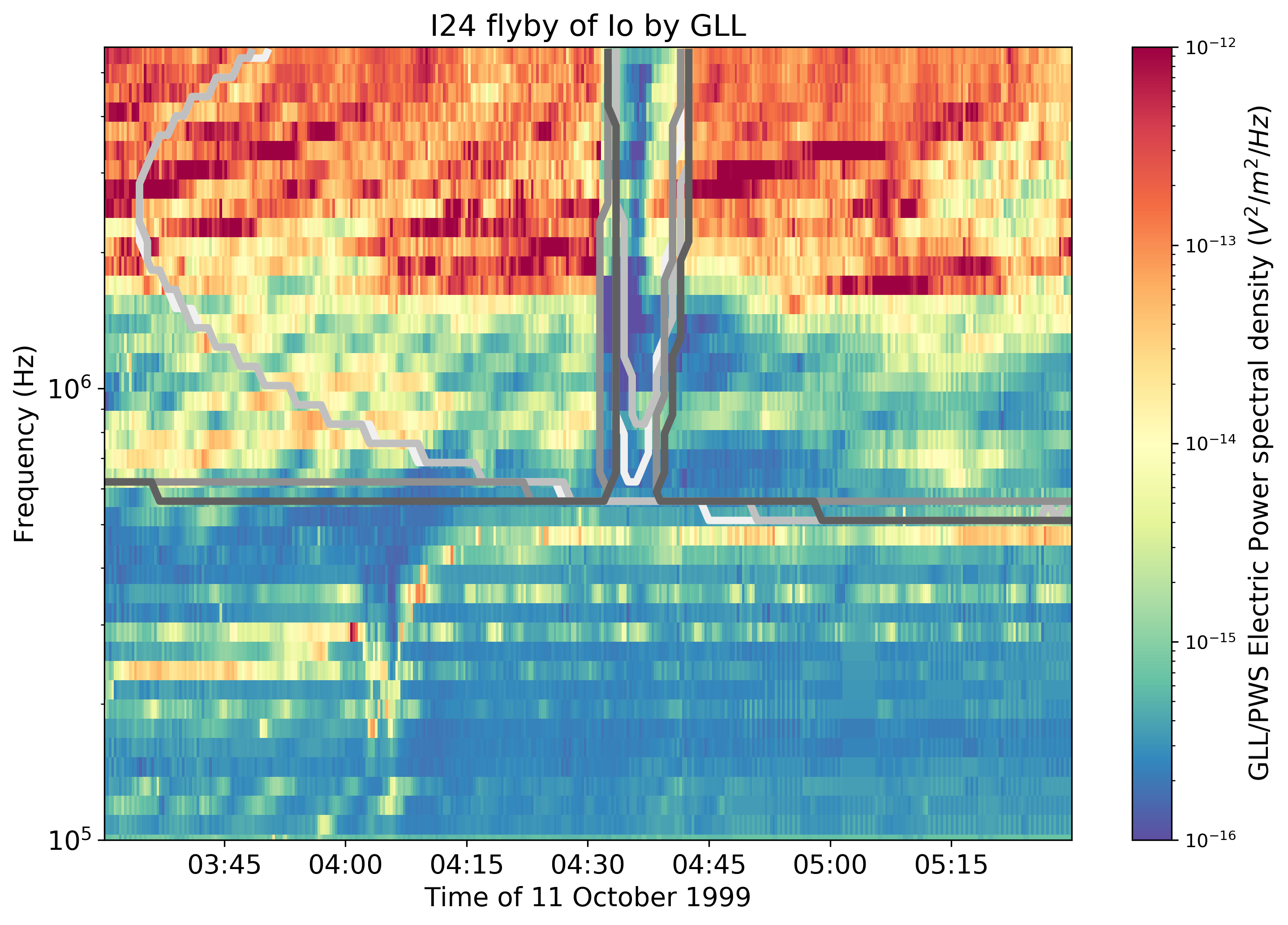
Figure 9: Superimposed GLL/PWS data and ExPRES simulations during Jovian radio emission occultations by Io (flyby I24). The four types of emission (A, B, C, D) are separated (from white to dark grey, resp.)

Figure 9 displays the occultation during the I24 Io’s flyby. At ingress, the occultation of the higher intensity is well modelled. We observe radio signals during the modelled full occultation, and the observed egress seems to occur earlier than the prediction. Intense radio arcs are visible above 2 MHz, showing the lower frequency part of vertex-late arcs. The radio signal is attenuated below 1 to 2 MHz, especially after the flyby. The $f_{UH}$ line is also observed ($\sim$300 kHz to $\sim$500 kHz). https://doi.org/10.25935/8zff-nx36#I24

This Io flyby also shows a noticeable feature. The modelled Northern radio sources (A and B, respectively in white and light-grey) are not observed at the beginning of the studied interval. This is due to the “Equatorial Shadow Zone” (ESZ) effect reported at Saturn (Lamy et al., 2008), see A for more details.

4.5 Other flybys

In the case of flybys with partial occultations (e.g., G02, G07, E11, E26 or G28), the Jovian radio signals are observed during the flyby, with no full occultation interval. During the G07 flyby, only D sources are occulted. The GLL/PWS data (see https://doi.org/10.25935/8zff-nx36#G07) shows an attenuation of the Jovian radio signals that fits the predicted occultation (see Figure 10), hence suggesting that several radio sources were active, including the D sources.

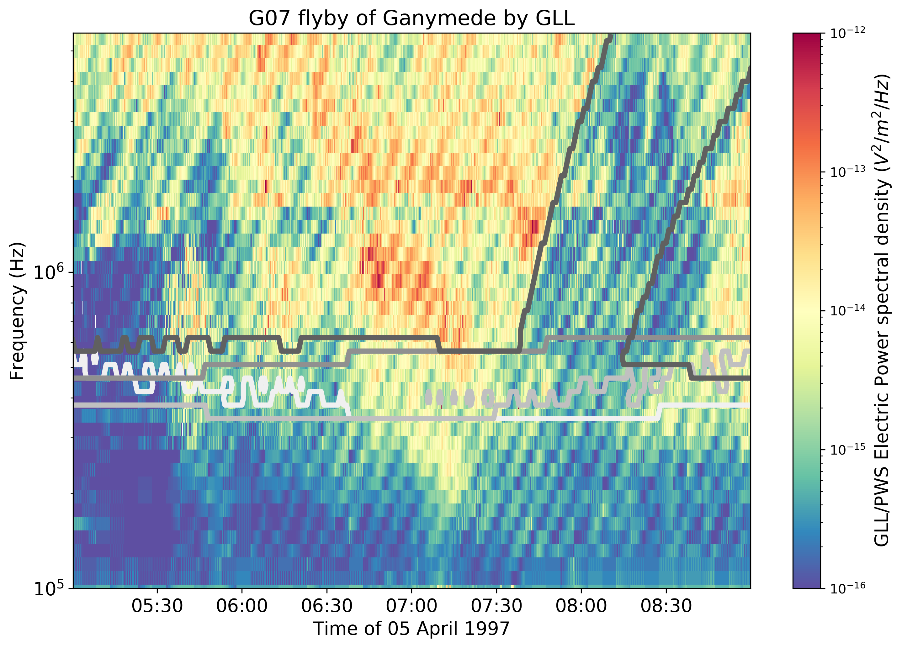
Figure 10: Superimposed Galileo PWS data and ExPRES simulations during Jovian radio emission occultations by Ganymede (flyby G07). The four types of emission (A, B, C, D) are separated (from white to dark grey, resp.)

Most of the other flybys (e.g., C03, E04, E06, G08, C10, E19) are occurring on the Jovian-facing side of the moon, where no occultation can occur.

5 Results and Discussion

5.1 Temporal Occurrence and Spectral Coverage of Jovian Auroral Radio Signals

The first result of this study is the fact that Jovian auroral radio emissions are present almost continuously, although this may not be obvious in some observational data sets, due to the limited sensitivity of instruments. Ground based radio telescopes (such as the Nançay Array, in France) provide the longest observation collections (Marques et al., 2017), but the distance to Jupiter limits the detection of low intensity events despite their intrinsic sensitivity. Space borne radio instruments (such as Voyager/PRA, Cassini/RPWS, GLL/PWS or Juno/Waves), provide observations from a closer range to Jupiter. Cassini and Galileo data show quasi-continuous radio signals (as shown on Figure 1). The ExPRES of auroral radio sources, configured with radio sources every 1^∘ in longitude, is consistent with this observation (with the noticeable exception of the ESZ, for an observer located around Io’s orbital distance to Jupiter).

The occultation analysis shows that all sources must be occulted in order to remove the natural radio signature of Jupiter’s magnetospheric activity. It is also noticeable that faint emissions are still visible during some occultations (e.g., during the G01, E12 and C30 Galileo flybys).

The JUICE/RPWI and RIME instruments will observe . The JUICE/RIME and Cassini/RPWS instruments have similar antenna characteristics, leading to an antenna resonance at about $\sim$9 MHz (Zarka et al., 2004; Bruzzone et al., 2013). It is thus very likely that JUICE/RIME will observe similar signals as those shown on Figure 1 (with a spectral range restricted around 9 MHz).

The low frequency limit is usually well predicted by ExPRES, as shown on Figures 5, 6, 7, 9 and 10. The ExPRES low frequency emission limit is determined by the CMI theory: the emission can occur only when $f_{pe}/f_{ce}<0.01$. This finding implies that our of the magnetic field and plasma density is consistent with the radio observations. Discrepancies (e.g., during flyby C30) may be related to the of the two aforementioned characteristic frequencies: $f_{pe}$ depends on the magnetospheric current sheet model; and $f_{ce}$ is determined by the magnetic field model. The JRM09 magnetic field model is derived from the Juno magnetic measurements in the polar regions of Jupiter. This model is thus perfectly adapted for our application. Conversely, the current sheet model could be improved. The results of this study will be and updated The effect of the Solar Wind conditions may also play a role (as studied by Hess et al., 2012)

5.2 Radio source location

Figure 11 displays the occultation of the Jovian radio sources during the flyby I24, for two sets of simulation runs. In the top and bottom panels, the sources are located on the magnetic field lines with an M-shell of 50 and 30 $R_{J}$, respectively, with the larger M-shell, corresponding to radio sources located at higher magnetic latitudes. We observe no difference for the occultation prediction.

The difference in the low cut-off frequency of the simulated emissions is very small (with a slightly lower low cut-off frequency for sources with M-shells of 50 $R_{J}$). The main difference is observed for the A and B sources (white and light-grey curve), with the ESZ feature occurring at a different time.

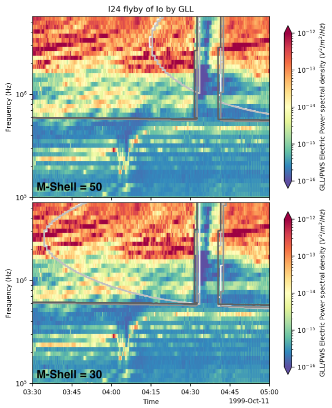
Figure 11: Comparison between the Jovian radio occultation during the I24 flyby for sources on magnetic field lines at M shell M=50 (top panel) and M=30 (bottom panel).

5.3 Occultation accuracy and propagation effects

The ExPRES modelling the observed occultation (e.g., C30 flyby, or E12 and I24 flyby ingress). The ExPRES simulation runs have been configured with a 1 minute sampling step, which sets the general temporal sampling of this study. The discrepancies between the predictions and observation have to be further studied. The mismatch mostly occurs at frequencies lower than $\sim$1 MHz. In this range, propagation effects (such as refraction effects) are known to occur, with, e.g., attenuation lanes. We observe them in all studied flybys, e.g., on E12, where the Jovian auroral radio waves are attenuated below $\sim$2 MHz, with an intensification at $\sim$1 MHz.

Flyby	Phase	Date Time (SCET)	Temporal accuracy (s)
G01	ingress	1996-06-27 06:00:00	55	45	32	19	13
G01	egress	1996-06-27 06:20:00	22	18	13	7	5
E12	ingress	1997-12-16 12:02:00	14	12	8	5	4
E12	egress	1997-12-16 12:12:00	29	24	17	11	8
I24	ingress	1999-10-11 04:33:00	23	19	14	9	6
I24	egress	1999-10-11 04:42:00	49	40	28	18	12
C30	ingress	2001-05-25 11:25:00	5	4	3	1	1
C30	egress	2001-05-25 11:50:00	26	20	15	8	5
Frequency (MHz)			0.7	1.0	2.0	5.0	10.0

Table 2: Estimation of the temporal uncertainty of the predicted occultation timing in seconds.

In the case of G01, the egress is observed several minutes after the predicted egress time. Figure 12 shows how the same observations can be interpreted considering refraction effects on the ionosphere of the moon.

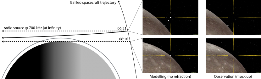
Figure 12: Sketch of G01 configuration, with a modelled radio source at 700 kHz, assumed to be at infinity on the left-hand side. The plain line is a sketched refracted ray path. The plain grey line represents the ionosphere of the moon. The dashed lines are the straight line propagation (no refraction) for the same source. Two locations of the Galileo spacecraft trajectory are illustrated on the right-hand side of the Figure. The “Modelling (no refraction)” column shows frames extracted from the G01 ‘pov’ movie at 06:16 and 06:21. The right-most column (“Observation”) shows at low frequencies.

In Figures 5, 6 and 7, we observe faint and sometimes sporadic radio signals, which are visible during the occultation interval, despite the predicted full occultation. Since the moon is geometrically occulting all the Jovian radio sources, refraction effects must be taken into account to interpret the observation. These effects can occur either in the moon’s atmosphere and ionosphere, in the Io plasma torus or in the magnetospheric plasma sheet. ExPRES assumes a straight line propagation between the radio source and the observer.

The two latter results (occultation ingress and egress prediction mismatch and faint signals during full occultation) indicate that propagation effects play an important role in the fine understanding of the Galilean radio occultations. Further analysis requires the coupling to a ray-tracing code, such as ARTEMIS-P (Anisotropic Ray Tracer for Electromagnetism in Magnetosphere, Ionosphere and Solar wind including Polarization, Gautier et al., 2013).

6 Usage for the JUICE mission planning tools

The science planning activity, coordinated by the JUICE Science Operations Center (JUICE SOC), relies on the identification, at each point in time, of the science opportunities, using science models or/and geometry. For JUICE, some of those depend on the Jupiter Radio emission simulation. Ionosphere active and/or passive radar sounding activities opportunities can benefit from an accurate simulation of Jupiter radio emission.

Since the ExPRES can provide as the of the radio sources as seen from the spacecraft for a range of frequencies (i.e., 1–40 MHz), the has implemented a standalone tool, which wraps the ExPRES and science opportunity windows based on the radio source position. This can be used to identify opportunity windows for one of the high priority science objectives of the RPWI instrument, the icy moon ionosphere through ionosphere refraction/distortion measurement.

The opportunity periods currently generated to drive the corresponding RPWI measurements are linked to the ingress and egress occultation events of the Jupiter , where at least one Jupiter radio sources with a frequency between 0.1–5 MHz crossing the moon ionosphere (with ).

In 13, the Jupiter auroral radio source as seen from JUICE during 21C13 (the last Callisto flyby of the tour) as a function of frequency (MHz) and UTC time is displayed: the red dots correspond to opportunity for ionosphere , i.e., whenever one of the radio source types (A, B, C or D) is seen by JUICE with a line of sight passing through the ionosphere within 0–100 km. This section is using the CReMA 3.0 trajectory scenario.

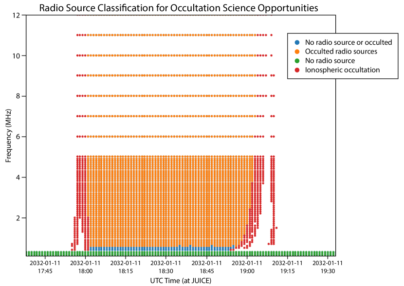
Figure 13: .

Figure 14 shows the resulting opportunities as a function of the spacecraft altitude in km (green background). There are a few gaps within the ingress and egress opportunities. Those gaps of 1-2 minutes are ignored to compute the final iono_ingress and iono_egress envelops used for the planning. Table 4 lists the RPWI in-situ and radio measurement sequence for the 21C13 scenario based on the Closest Approach (CA), and the ingress and egress windows envelope for ionosphere . .

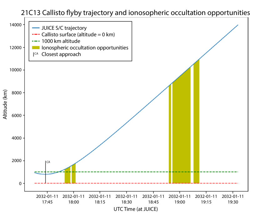
Figure 14: spacecraft in km for the 21C13 Flyby (blue line); surface (resp. the 1000km altitude above surface) is represented by the red dashed line (resp. green dashed line), and the ionosphere opportunities windows are filled in background.

	Date Time	Frequency	Altitude	Velocity	Uncertainty
Event	(SCET)	(MHz)	(km)	(km/s)	(s)
Full Occ. Start	2032-01-11 18:00:22	10.0	1686.7	2.88	5
Full Occ. End	2032-01-11 19:03:22	10.0	9880.1	2.45	18

Table 3:

UTC Date & Time	Reference Event	Relative Time	In-situ	Radio
2032-01-11T05:44:05	CA	$-$12:00:00	slow	full
2032-01-11T08:14:05	CA	$-$09:30:00	normal	full
2032-01-11T17:34:05	CA	$-$00:10:00	burst	full
2032-01-11T17:54:05	CA	$+$00:10:00	normal	full
2032-01-11T17:55:00	iono_ingress	$+$00:00:00	normal	burst
2032-01-11T18:01:00	iono_egress	$+$00:00:00	normal	full
2032-01-11T18:54:00	iono_ingress	$+$00:00:00	normal	burst
2032-01-11T19:11:00	iono_egress	$+$00:00:00	normal	full
2032-01-12T03:14:05	CA	$+$09:30:00	slow	full
2032-01-12T05:44:05	CA	$-$12:00:00	slow	full

Table 4: RPWI in-situ and radio observations mode sequence during the 21C13 Callisto flyby scenario. Some mode changes are scheduled w.r.t. Closest Approach event (CA), while ionosphere observations are scheduled w.r.t. ingress and egress events as identified using Express.

figure 15 is a screenshot of this measurement as shown by the JUICE SOC Mapping and Planning Payload Science software (MAPPS), used to simulate the spacecraft and payload status (i.e., power, data rate, on-board mass memory (SSMM)). The RPWI operations are planned around the CA and around ingress and egress ionosphere opportunities as described in Table 4. The high-resolution in-situ measurement mode is scheduled +/- 10 minutes around the closest approach (CA), while the high resolution radio measurement mode is scheduled during the ionosphere opportunities. High-resolution modes are the demanding in term of resources (power, data generated, stored in SSMM and to be downloaded (data rate)) and are reserved for priority scientific objectives. So it is crucial to be able to calculate the corresponding opportunities windows.

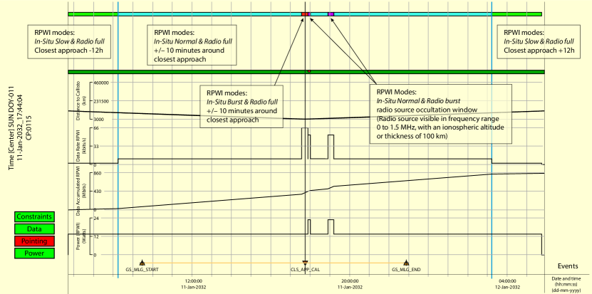
Figure 15:

The JUICE mission is in development phase, with a planned launch in 2022. At this stage the JUICE mission science planning process is being exercised by analysing representative science scenarios similar to 21C13. In this study, the scenario analysis covers $\pm$12 hours around the Callisto closest approach. . The JUICE SOC the same type of opportunity windows whenever a new candidate trajectory is available for JUICE.

The results can also be useful for other , and will be made available JUICE SOC instrument teams. This includes the measurement linked to the icy shell characterisation of the icy moons:

• Passive radar measurement by or by RPWI: Opportunities can be identified whenever any radio source is visible from the spacecraft for any source type (), and per source type (to differentiate source from northern and southern hemispheres) between 1 and 40 MHz (although lower frequencies are better );

• Active Radar measurement by : when the spacecraft is protected from Jupiter radio emission due to moon occultation for sources with frequency between 9 and 11 MHz (i.e., flybys and Ganymede phase) and when the spacecraft is within the RIME instrument operating range (altitude $<$1000 km).

7 Conclusions and Perspectives

The Galileo radio occultations observed the PWS data set are well modelled by ExPRES simulation, with a sampling of the order of one minute. Discrepancies between predicted and observed ingress or egress times can be attributed to refraction effects, which are not included in the current modelling scheme. The validation on GLL/PWS data allows us to apply the same modelling to the JUICE mission planning, in order to support the scientific segmentation of the Galilean moon flybys. The ExPRES modelling will also be useful for data analysis of “passive radar” observations, since it provides the location of the Jovian radio sources used to probe the moon’s sub-surface.

On a technical point of view, the JUICE modelling have been done running ExPRES through the PADC operated UWS interface based on OPUS. This framework is fully adapted to the usage presented in this study. Future developments of the ExPRES code and its implementation at PADC will include better management of Provenance metadata (Servillat et al., 2020, 2021b), to enhance the scientific traceability and reproducibility of the results.

Several means of refining the occultation modelling have been identified. The main one is involving ray-tracing in the Jovian system (mainly the Io Torus) and the moon’s environment. This extra modelling step requires models of the magnetic field and plasma density environments in the vicinity of the studied moon, including the magnetospheric and moon contributions (see, e.g., Modolo et al., 2018). A second order improvement may also be provided by the use of a more accurate magnetospheric current sheet model, which will refine the location of the radio sources on the low frequency end.

Appendix A Equatorial Shadow Zone

In the equatorial region, in the innermost magnetosphere, the auroral radio sources are not visible, due to combination of the shape of the radio emission beaming patterns and the topology of the magnetic field lines bearing the radio source. This effect is named “Equatorial Shadow Zone” (ESZ). This effect has been identified at Saturn (Lamy et al., 2008), using a preliminary version of the ExPRES code. It has also been observed at Earth (see, e.g., Morioka et al., 2011, Figure 1), but not explicitly described.

Our simulation runs show that some of the Jovian auroral radio sources are not always visible at the distance of Io’s orbit. Figure 16 shows the observability for each auroral radio source for an observer located on Io’s orbit, during one rotation of Jupiter. The simulation shows that the Southern radio sources (namely, the C and D source) are not visible in the CML range 180 to 210 degrees. The Northern radio sources (namely, the A and B source) are observable from all CML, with a drastically reduced spectral range at a CML of about 25 degrees. Since the Northern and Southern ESZs do not occur at the same time, an observer will not experience a full dropout of radio signals, to what is observed at Saturn.

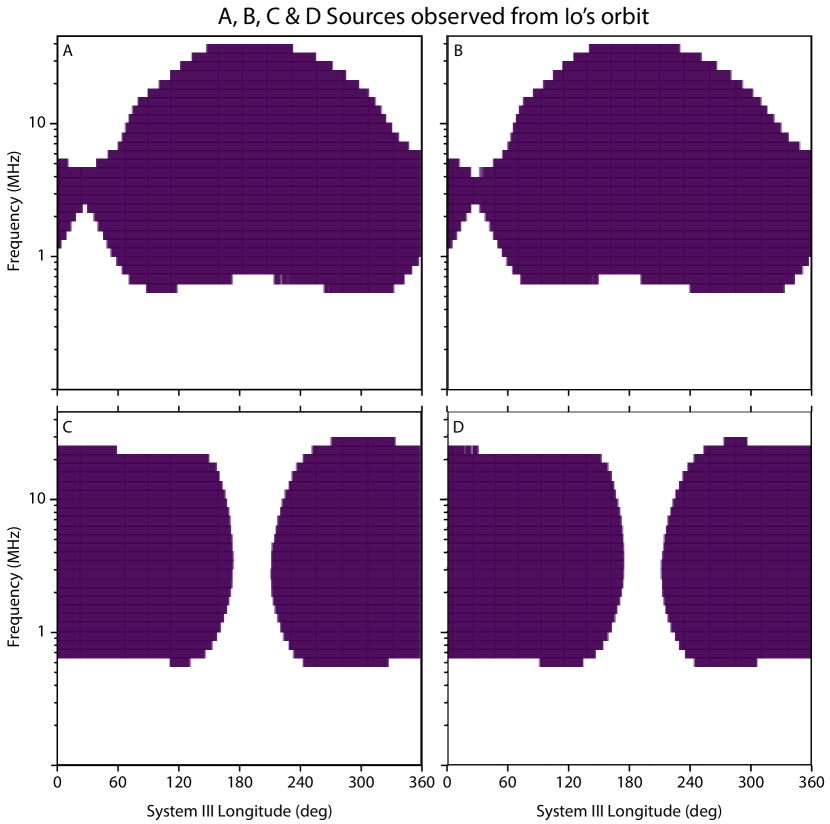
Figure 16: Jovian auroral radio source observability from Io’s orbit.

Appendix B Radio source location uncertainty

Figure 17: Radio sources location shifts (in Jovian radii) with varying M-shell (from 10 to 50 $R_{J}$), as a function of longitude, for the Northern (solid line) and Southern (dotted-dashed line) hemispheres, at different frequencies: 700 kHz (blue), 1 MHz (green), 2 MHz (red), 5 MHz (yellow) and 10 MHz (purple).

	Angular uncertainty (deg)
Moon	700 kHz	1 MHz	2 MHz	5 MHz	10 MHz
Io	4.3	3.5	2.5	1.6	1.1
Europa	2.7	2.2	1.6	1.0	0.7
Ganymede	1.7	1.4	1.0	0.6	0.4
Callisto	1.0	0.8	0.6	0.3	0.2

Table 5: Angular uncertainty (in degrees) of Jovian radio sources location for M-shells, as observed from each Galilean moons and for a set of 5 frequencies from 700 kHz to 10 MHz).

Appendix C Evaluation of refraction effects

Moon	$n_{0}\,(\textrm{cm}^{-3})$	$h_{0}\,(\textrm{km})$	Reference
Europa	9000	250	Kliore (1998)
Ganymede	400	600	Gurnett et al. (1996)
Ganymede	2200	125	Eviatar et al. (2001)
Callisto	10000	30	Hartkorn (2017)

Table 6: Plasma environment model parameters (reference density $n_{0}$ and scale height $h_{0}$) for Europa, Ganymede and Callisto.

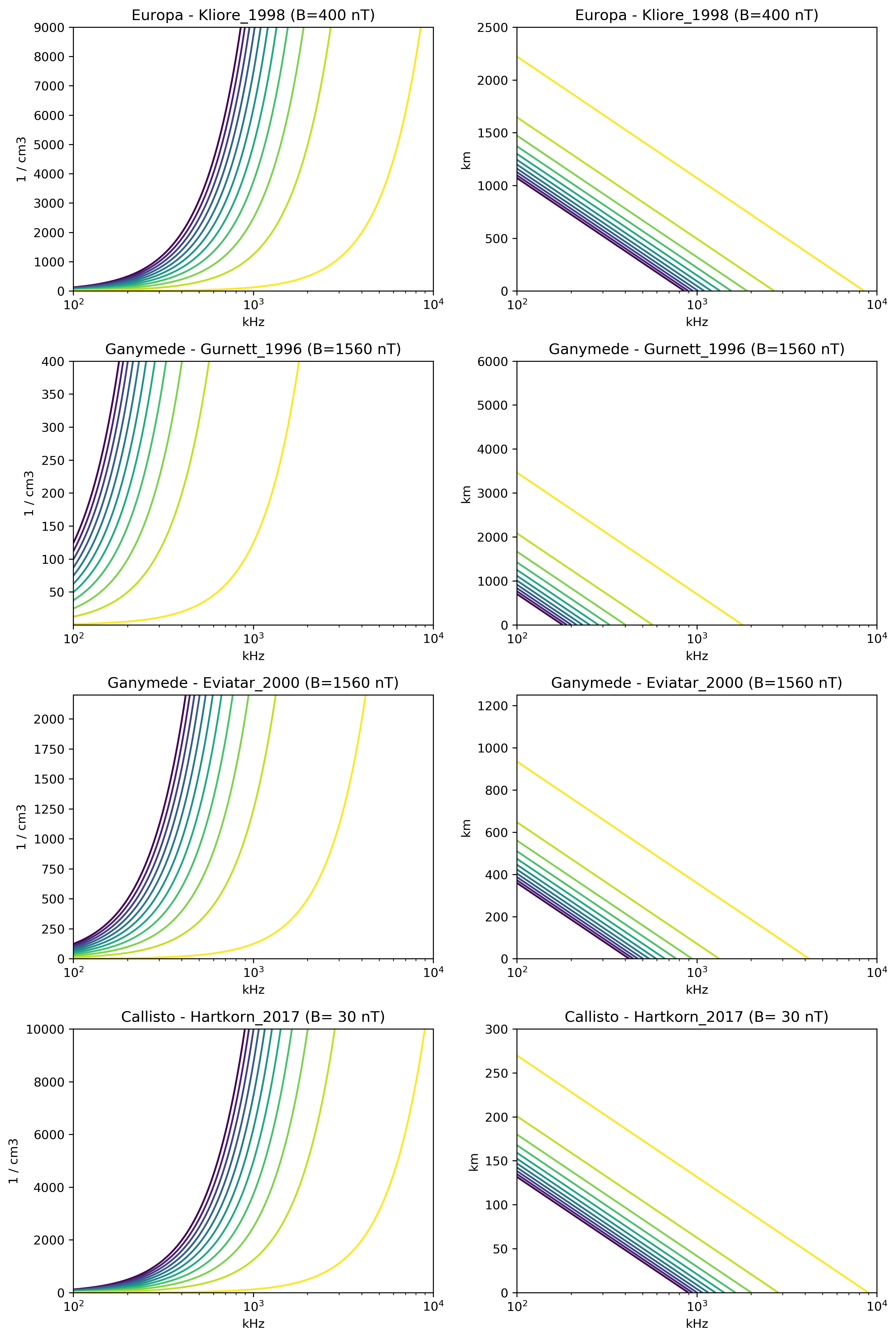
Figure 18: Contours of the refractive index values ($n^{2}$), for each selected environment models, with 11 contour levels at 0.0, 0.1, 0.2… 0.9 and 0.99, from left (purple) to right (yellow). From top to bottom: Europa with Kliore (1998), Ganymede with Gurnett et al. (1996) or Eviatar et al. (2001), and Callisto with Hartkorn (2017). The left-hand side columns shows the contour in the plasma density versus frequency space. The right-hand side column shows the altitude versus frequency space.

		Frequency (MHz)
Quantity	Moon (Reference)	0.7	1	2	5	10	Unit
Plasma Density	all	60	125	500	3000	12500	cm-3
Altitude	Europa (Kliore, 1998)	1250	1000	720	270	–	km
Altitude	Ganymede (Gurnett et al., 1996)	1100	700	–	–	–	km
Altitude	Ganymede (Eviatar et al., 2001)	450	360	180	–	–	km
Altitude	Callisto (Hartkorn, 2017)	150	130	90	35	–	km

Table 7: Estimated parameter thresholds accessible with low frequency radio occultations. The plasma density threshold is a lower limit, while the altitude threshold is an upper limit. Missing values (–) correspond to situations where no refraction is expected, considering no significant refraction occurs for $n^{2}>0.99$.

Appendix D Supplementary Material Description

The material used to conduct the Galileo flybys’ study are provided as a separate data collection (Cecconi et al., 2021, available at https://doi.org/10.25935/8zff-nx36) hosted by PADC (Paris Astronomical Data Centre). For each flyby, . The content of is described below.

D.1 ExPRES products

The ExPRES data set is composed of four files: (a) an ExPRES configuration file (JSON format), (b) a Galileo spacecraft ephemeris data exported from WebGeoCalc (CSV format), (c) the output ExPRES simulation run data (CDF format), and (d) the observed GLL/PWS data with the superimposed occultation contours (PNG format). Files (a) and (b) contains the ExPRES parameters and the SPICE Kernels used for the simulation, ensuring the results are reproducible.

D.2 Cosmographia context products

The Cosmographia data set is composed of a series of subdirectories, organised according to Cosmographia’s documentation. It contains all the required configuration catalogue files: the SPICE catalogue file listing the kernels in use for a scene; the spacecraft catalogue file defining the time interval of the scene and the spacecraft reference frame; the modelled radio source catalogue file, derived from an ExPRES simulation run; the ExPRES configuration file and simulation run; and the scripts used to produce the movie output. Two output movies are provided, showing the flyby scenes, as seen from the spacecraft (‘pov’ labelled movie) and from the top of the Jovian system (‘top’ labelled movie).

References

- Acton et al. (2018) Charles Acton, Nathaniel Bachman, Boris Semenov, and Edward Wright. A look towards the future in the handling of space science mission geometry. Planet. Space Sci., 150:9–12, 2018. doi: 10.1016/j.pss.2017.02.013.
- Acton (1996) Charles H. Acton. Ancillary data services of NASA’s Navigation and Ancillary Information Facility. Planet. Space Sci., 44(1):65–70, January 1996. doi: 10.1016/0032-0633(95)00107-7.
- Appleton (1932) E Appleton. Wireless studies of the ionosphere. Proceedings of the Wireless Section, Institution of Electrical Engineers, 7(21):257, 1932.
- Bruzzone et al. (2013) L Bruzzone, J J Plaut, G Alberti, D D Blankenship, F Bovolo, B A Campbell, A Ferro, Y Gim, W Kofman, G Komatsu, W McKinnon, G Mitri, R Orosei, G W Patterson, D Plettemeier, and R Seu. RIME: RADAR FOR ICY MOON EXPLORATION. 2013 IEEE International Geoscience and Remote Sensing Symposium - IGARSS, pages 3907–3910, July 2013. doi: 10.1109/IGARSS.2013.6723686.
- Burke and Franklin (1955) BF Burke and KL Franklin. Observations of a Variable Radio Source Associated with the Planet Jupiter. J. Geophys. Res., 60:213–217, 1955. doi: 10.1029/JZ060i002p00213.
- Cecconi et al. (2012) B Cecconi, SLG Hess, A Hérique, Maria Rosaria Santovito, Daniel Santos-Costa, Philippe Zarka, G Alberti, DD Blankenship, Jean-Louis Bougeret, L Bruzzone, and W Kofman. Natural radio emission of Jupiter as interferences for radar investigations of the icy satellites of Jupiter. Planet. Space Sci., 61:32–45, 2012. doi: 10.1016/j.pss.2011.06.012.
- Cecconi (2019) Baptiste Cecconi. Workflow studies: Magnetospheres science and support to ESA/JUICE mission planning, January 2019.
- Cecconi and Zarka (2019) Baptiste Cecconi and Philippe Zarka. Cassini rpws jupiter encounter calibrated dataset v1.0 [dataset]. PADC, 2019. doi: 10.25935/H98J-MA66.
- Cecconi et al. (2020) Baptiste Cecconi, Alan Loh, Pierre Le Sidaner, Renaud Savalle, Xavier Bonnin, Quynh Nhu Nguyen, Sonny Lion, Albert Shih, Stéphane Aicardi, Philippe Zarka, Corentin Louis, Andrée Coffre, Laurent Lamy, Laurent Denis, Jean-Mathias Grießmeier, Jeremy Faden, Chris Piker, Nicolas André, Vincent Génot, Stéphane Erard, Joseph N Mafi, Todd A King, Jim Sky, and Markus Demleitner. MASER: A Science Ready Toolbox for Low Frequency Radio Astronomy. Data Science Journal, 19(18):1062, 2020. doi: 10.5334/dsj-2020-012.
- Cecconi et al. (2021) Baptiste Cecconi, Corentin Louis, Claudio Muñoz Crego, and Claire Vallat. Auroral radio source occultation modeling and application to the juice science mission planning. supplementary material: Galileo flybys [dataset]. PADC, 2021. doi: 10.25935/8ZFF-NX36.
- Colin (1972) Lawrence Colin. Mathematics of Profile Inversion. Technical Report NASA-TM-X-62150, NASA, 1972.
- Connerney et al. (1981) J. E. P. Connerney, M. H. Acuna, and N. F. Ness. Modeling the Jovian current sheet and inner magnetosphere. J. Geophys. Res., 86:8370–8384, September 1981. doi: 10.1029/JA086iA10p08370.
- Connerney et al. (2018) J E P Connerney, S Kotsiaros, R J Oliversen, J R Espley, J L Joergensen, P S Joergensen, J M G Merayo, M Herceg, J Bloxham, K M Moore, S J Bolton, and S M Levin. A New Model of Jupiter’s Magnetic Field From Juno’s First Nine Orbits. Geophys. Res. Lett., 45(6):2590–2596, 2018. doi: 10.1002/2018GL077312.
- Connerney et al. (2020) J E P Connerney, S Timmins, M Herceg, and J L Joergensen. A Jovian Magnetodisc Model for the Juno Era. J. geophys. Res. Space Physics, 125:1–11, September 2020.
- ESA SPICE Service (2020) ESA SPICE Service. JUICE SPICE Kernel Dataset, V2.7 [Dataset]. ESA, 2020. doi: 10.5270/esa-ybmj68p.
- Eviatar et al. (2001) A Eviatar, V M Vasyliunas, and D Gurnett. The ionosphere of Ganymede. Planet. Space Sci., 49:327–336, 2001. doi: 10.1016/S0032-0633(00)00154-9.
- Gautier et al. (2013) Anne-Lise Gautier, Baptiste Cecconi, and Philippe Zarka. ARTEMIS-P: A general Ray Tracing code in anisotropic plasma for radioastronomical applications. Proceedings of the 2013 International Symposium on Electromagnetic Theory, pages 1–4, 2013.
- Grodent (2015) Denis Grodent. A Brief Review of Ultraviolet Auroral Emissions on Giant Planets. Space Sci. Rev., 187:23–50, 2015. doi: 10.1007/s11214-014-0052-8.
- Gurnett et al. (1996) D A Gurnett, W S Kurth, A Roux, S J Bolton, and C F Kennel. Evidence for a magnetosphere at Ganymede from plasma-waves observations by the Galileo spacecraft. Nature, 384:535–537, 1996. doi: 10.1038/384535a0.
- Gurnett et al. (1997) D. A. Gurnett, W. S. Kurth, and L. J. Granroth. GO J PWS REFORMATTED PLAYBACK SPECTRUM ANALYZER FULL V1.0 [Dataset]. NASA Planetary Data System, GO-J-PWS-2-REDR-LPW-SA-FULL-V1.0, 1997. doi: 10.17189/1519681.
- Gurnett et al. (2004) D A Gurnett, W S Kurth, D L Kirchner, G B Hospodarsky, T F Averkamp, P Zarka, A lecacheux, R. Manning, A Roux, P Canu, N Cornilleau-Wehrlin, P Galopeau, A Meyer, R Bostrom, G Gustafsson, J-E Wahlund, L Âhlen, H O Rucker, H. P. Ladreiter, W Macher, L J C Woolliscroft, H Alleyne, M L Kaiser, M D Desch, W M Farrell, C C Harvey, P Louarn, P J Kellogg, K Goetz, and A Pedersen. The Cassini Radio and Plasma Wave Investigation. Space Sci. Rev., 114(1-4):395–463, 2004. doi: 10.1007/s11214-004-1434-0.
- Gurnett et al. (1992) DA Gurnett, William S Kurth, RR Shaw, A Roux, R Gendrin, CF Kennel, FL Scarf, and SD Shawhan. The Galileo plasma wave investigation. Space Sci. Rev., 60:341–355, 1992. doi: 10.1007/BF00216861.
- Gurnett et al. (1998) DA Gurnett, William S Kurth, JD Menietti, and AM Persoon. An unsual rotationally modulated attenuation band in the Jovian hectometric radio emission spectrum. Geophys. Res. Lett., 25(11):1841–1844, 1998. doi: 10.1029/98GL01400.
- Harrison and Rixon (2016) P. A. Harrison and G. Rixon. Universal Worker Service Pattern Version 1.1. page 1024, October 2016. doi: 10.5479/ADS/bib/2016ivoa.spec.1024H.
- Hartkorn (2017) Olivier Hartkorn. Modeling Callisto’s Ionosphere, Airglow and Magnetic FieldEnvironment. Technical report, Köln Universität, July 2017.
- Hess et al. (2012) S L G Hess, E Echer, and P Zarka. Solar wind pressure effects on Jupiter decametric radio emissions independent of Io. Planetary and Space Science, 70(1):114–125, 2012. doi: 10.1016/j.pss.2012.05.011.
- Kliore (1998) A J Kliore. Satellite atmosphere and magnetosphere. Highlights of Astronomy, 11B:1065–1069, 1998.
- Kumamoto et al. (2017) A. Kumamoto, Y. Kasaba, F. Tsuchiya, H. Misawa, H. Kita, W. Puccio, J. E. Wahlund, J. Bergman, B. Cecconi, Y. Goto, J. Kimura, and T. Kobayashi. Feasibility of the exploration of the subsurface structures of Jupiter’s icy moons by interference of Jovian hectometric and decametric radiation. In G. Fischer, G. Mann, M. Panchenko, and P. Zarka, editors, Planetary Radio Emissions VIII, pages 127–136, Jan 2017. doi: 10.1553/PRE8s127.
- Kurth et al. (1997) William S Kurth, S J Bolton, D A Gurnett, and S Levin. A Determination of the source of the Jovian hectometric radiation via occultation by Ganymede. Geophys. Res. Lett., 24(10):1171–1174, 1997. doi: 10.1029/97GL00988.
- Lamy et al. (2008) L Lamy, Philippe Zarka, B Cecconi, SLG Hess, and Renée Prangé. Modeling of Saturn Kilometric Radiation arcs and equatorial shadow zone. J. Geophys. Res., 113(A10213), 2008. doi: 10.1029/2008JA013464.
- Lamy et al. (2017) L. Lamy, P. Zarka, B. Cecconi, L. Klein, S. Masson, L. Denis, A. Coffre, and C. Viou. 1977-2017: 40 years of decametric observations of Jupiter and the Sun with the Nancay Decameter Array. In G. Fischer, G. Mann, M. Panchenko, and P. Zarka, editors, Planetary Radio Emissions VIII, pages 455–466, Jan 2017. doi: 10.1553/PRE8s455.
- Louarn et al. (1997) P Louarn, S Perraut, A Roux, DA Gurnett, William S Kurth, and SJ Bolton. Global plasma environment of Io as inferred from the Galileo plasma wave observations. Geophys. Res. Lett., 24:2115, 1997.
- Louarn et al. (2017) P Louarn, F Allegrini, D J McComas, P W Valek, W S Kurth, N André, F Bagenal, S Bolton, J Connerney, R W Ebert, M Imai, S Levin, J R Szalay, S Weidner, R J Wilson, and J L Zink. Generation of the Jovian hectometric radiation: First lessons from Juno. Geophys. Res. Lett., 44(10):4439–4446, 2017. doi: 10.1002/2017GL072923.
- Louarn et al. (2018) P Louarn, F Allegrini, D J McComas, P W Valek, W S Kurth, N André, F Bagenal, S Bolton, R W Ebert, M Imai, S Levin, J R Szalay, and R J Wilson. Observation of Electron Conics by Juno: Implications for Radio Generation and Acceleration Processes. Geophys. Res. Lett., 45:9408–9416, October 2018.
- Louis et al. (2019a) C K Louis, S L G Hess, B Cecconi, P Zarka, L Lamy, S Aicardi, and A Loh. ExPRES: an Exoplanetary and Planetary Radio Emissions Simulator. Astron. and Astrophys., 627:A30, 2019a. doi: 10.1051/0004-6361/201935161.
- Louis et al. (2019b) C K Louis, R Prangé, L Lamy, P Zarka, M Imai, W S Kurth, and J E P Connerney. Jovian Auroral Radio Sources Detected In Situ by Juno/Waves: Comparisons With Model Auroral Ovals and Simultaneous HST FUV Images. Geophys. Res. Lett., 46:11606–11614, October 2019b.
- Louis et al. (2020) Corentin K. Louis, Sébastien L. G. Hess, Baptiste Cecconi, Philippe Zarka, Laurent Lamy, Stéphane Aicardi, and Alan Loh. maserlib/expres: Version 1.1.0 [software]. Zenodo, 2020. doi: 10.5281/zenodo.4292002.
- Marques et al. (2017) M. S. Marques, P. Zarka, E. Echer, V. B. Ryabov, M. V. Alves, L. Denis, and A. Coffre. Statistical analysis of 26 yr of observations of decametric radio emissions from Jupiter. Astron. Astrophys., 604:A17, 2017. doi: 10.1051/0004-6361/201630025.
- Menietti et al. (2003) JD Menietti, DA Gurnett, GB Hospodarsky, CA Higgins, William S Kurth, and Philippe Zarka. Modeling radio emission attenuation lanes observed by the Galileo and Cassini spacecraft. Planet. Space Sci., 51:533–540, 2003. doi: 10.1016/S0032-0633(03)00078-3.
- Modolo et al. (2018) R Modolo, S Hess, V Génot, L Leclercq, F Leblanc, J Y Chaufray, P Weill, M Gangloff, A Fedorov, E Budnik, M Bouchemit, M Steckiewicz, N André, L Beigbeder, D Popescu, J P Toniutti, T Al-Ubaidi, M Khodachenko, D Brain, S Curry, B Jakosky, and M Holmström. The LatHyS database for planetary plasma environment investigations: Overview and a case study of data/model comparisons . Planetary and Space Science, 150:13–21, 2018. doi: 10.1016/j.pss.2017.02.015.
- Morioka et al. (2011) A Morioka, Y Miyoshi, F Tsuchiya, H Misawa, Y Kasaba, T Asozu, S Okano, A Kadokura, N Sato, H Miyaoka, K Yumoto, G. K. Parks, F Honary, Jean-Gabriel Trotignon, Pierrette Décréau, and B. W. Reinisch. On the simultaneity of substorm onset between two hemispheres. Journal of Geophysical Research Space Physics, 116:A04211 (15 pages), 2011. doi: 10.1029/2010JA016174.
- Piker et al. (2019) C Piker, L Granroth, J Mukherjee, D Pisa, B Cecconi, A Kopf, and J Faden. Lightweight federated data networks with das2 tools. Earth and Space Science Open Archive, 2019. doi: 10.1002/essoar.10500359.1.
- Romero-Wolf et al. (2015) Andrew Romero-Wolf, Steve Vance, Frank Maiwald, Essam Heggy, Paul Ries, and Kurt Liewer. A Passive Probe for Subsurface Oceans and Liquid Water in Jupiter’s Icy Moons. Icarus, 248:463–477, 2015. doi: 10.1016/j.icarus.2014.10.043.
- Schroeder et al. (2016) Dustin M Schroeder, Andrew Romero-Wolf, Leonardo Carrer, Cyril Grima, Bruce A Campbell, Wlodek Kofman, Lorenzo Bruzzone, and Donald D Blankenship. Assessing the potential for passive radio sounding of Europa and Ganymede with RIME and REASON. Planet. Space Sci., 134(C):52–60, 2016. doi: 10.1016/j.pss.2016.10.007.
- Servillat et al. (2020) Mathieu Servillat, Kristin Riebe, Catherine Boisson, François Bonnarel, Anastasia Galkin, Mireille Louys, Markus Nullmeier, Nicolas Renault-Tinacci, Michèle Sanguillon, and Ole Streicher. IVOA Provenance Data Model Version 1.0. page 411, April 2020.
- Servillat et al. (2021a) Mathieu Servillat, Stéphane Aicardi, Baptiste Cecconi, and Marco Mancini. OPUS: an interoperable job control system based on VO standards. arXiv e-prints, art. arXiv:2101.08683, January 2021a.
- Servillat et al. (2021b) Mathieu Servillat, François Bonnarel, Mireille Louys, and Michèle Sanguillon. Practical Provenance in Astronomy. arXiv e-prints, art. arXiv:2101.08691, January 2021b.
- Wahlund (2013) J. E. Wahlund. The Radio & Plasma Wave Investigation (RPWI) for JUICE. In European Planetary Science Congress, pages EPSC2013–637, September 2013.
- Witasse (2019) Olivier Witasse. JUICE (Jupiter Icy Moon Explorer): A European mission to explore the emergence of habitable worlds around gas giants. In EPSC-DPS Joint Meeting 2019, volume 2019, pages EPSC–DPS2019–400, 2019.
- Zarka (2004) P Zarka. Radio and plasma waves at the outer planets. Advances in Space Research, 33(11):2045–2060, January 2004.
- Zarka et al. (2004) Philippe Zarka, B Cecconi, and William S Kurth. Jupiter’s low-frequency radio spectrum from Cassini/Radio and Plasma Wave Science (RPWS) absolute flux density measurements. J. Geophys. Res., 109:A09S15, 2004. doi: 10.1029/2003JA010260.