On Riemannian Stochastic Approximation Schemes with Fixed Step-Size

Abstract

This paper studies fixed step-size stochastic approximation (SA) schemes, including stochastic gradient schemes, in a Riemannian framework. It is motivated by several applications, where geodesics can be computed explicitly, and their use accelerates crude Euclidean methods. A fixed step-size scheme defines a family of time-homogeneous Markov chains, parametrized by the step-size. Here, using this formulation, non-asymptotic performance bounds are derived, under Lyapunov conditions. Then, for any step-size, the corresponding Markov chain is proved to admit a unique stationary distribution, and to be geometrically ergodic. This result gives rise to a family of stationary distributions indexed by the step-size, which is further shown to converge to a Dirac measure, concentrated at the solution of the problem at hand, as the step-size goes to $0$. Finally, the asymptotic rate of this convergence is established, through an asymptotic expansion of the bias, and a central limit theorem.

1 INTRODUCTION

This paper deals with the study of fixed step-size Stochastic Approximation (SA) algorithms (Robbins and Monro,, 1951; Kushner and Yin,, 2003; Polyak and Juditsky,, 1992), defined on a Riemannian manifold $\Theta$ with metric $\mathfrak{g}$. Specifically, consider the problem

$$\text{find }\theta\in\Theta\text{ satisfying }h(\theta)=0\;,$$ (1)

$$\text{for a vector field $h:\Theta\to\mathrm{T}\Theta$}\;,$$

where $\mathrm{T}\Theta$ denotes the tangent bundle of $\Theta$, and $h$ is only accessible through an oracle returning noisy estimates. The setting where $h=-\mathrm{grad}\,f$ is of particular interest for minimizing a smooth function $f:\Theta\to\mathbb{R}$. In the Euclidean setting, Stochastic Gradient Descent (SGD) and its variants are now common methods for solving this problem (Bottou,, 2010; Bottou and Bousquet,, 2008). However, it should be stressed that (LABEL:eq:sa_pb) encompasses several other applications in stochastic optimization, reinforcement learning or maximum likelihood estimation, such as online Expectation Maximization algorithms (Cappé and Moulines,, 2009), policy gradient (Baxter and Bartlett,, 2001) or Q-learning (Jaakkola et al.,, 1993). Minimization over a Riemannian manifold or its general formulation (LABEL:eq:sa_pb) arises in many applications: Principal Component Analysis (Edelman et al.,, 1998), dictionary recovery (Sun et al.,, 2017), matrix completion (Boumal and Absil,, 2011), smooth semidefinite programs (Boumal et al.,, 2016), tensor factorization (Ishteva et al.,, 2011), and Riemannian barycenter estimation (Said and Manton,, 2019; Arnaudon et al.,, 2012). This has motivated the development of a comprehensive framework for stochastic optimization problems on Riemannian manifolds. One of the first contributions in this field is Bonnabel, (2013), which derives asymptotic convergence results for SA on Riemannian manifolds. Non-asymptotic results are obtained by Zhang and Sra, (2016) for a geodesically convex function $f$. This study has been followed and completed by Zhang et al., (2016); Sato et al., (2019) which introduce and analyze a Riemannian counterpart of the Stochastic Variance Reduced Gradient (SVRG) algorithm. Since then, many existing methods or results from the Euclidean case have been considered in a Riemannian setting. For example, Khuzani and Li, (2017) suggest a Riemannian stochastic primal-dual algorithm and most recently Tripuraneni et al., (2018) study an averaged version of Riemannian SGD.

In this paper, we are interested in the study of fixed step-size SA methods of the form

$$\theta_{n+1}=\operatorname{proj}_{\mathsf{S}}\left[\mathrm{Exp}_{\theta_{n}}\left\{\upeta H_{\theta_{n}}(X_{n+1})\right\}\right]\;,\;$$ (2)

$$\text{where}\;H_{\theta_{n}}(X_{n+1})=h(\theta_{n})+e_{\theta_{n}}(X_{n+1})\;.$$

In (2), $\upeta>0$ is a step-size, $(X_{n})_{n\in\mathbb{N}^{*}}$ is an $(\mathcal{F}_{n})_{n\in\mathbb{N}}$-adapted process, defined on a filtered probability space, with values in a measurable space $(\mathsf{X},\mathcal{X})$, and $e:\Theta\times\mathsf{X}\to\mathrm{T}\Theta$ is a measurable function, such that $\theta\mapsto e_{\theta}(x)$ is a vector field over $\Theta$, for any $x\in\mathsf{X}$. In addition, $\mathrm{Exp}_{\theta}:\mathrm{T}_{\theta}\Theta\to\Theta$ is the Riemannian exponential mapping and $\operatorname{proj}_{\mathsf{S}}:\Theta\to\mathsf{S}$ is a projection-like operator onto a subset $\mathsf{S}\subset\Theta$. This recursion is a natural extension of Euclidean SA, akin to the Robbins-Monroe algorithm, in a Riemannian setting.

In the Euclidean setting, the study of fixed step-size SA, and in particular SGD, has recently attracted much attention, see e.g. Ma et al., (2018); Vaswani et al., (2019); Dieuleveut et al., (2017); Bach, (2020); Bach and Moulines, (2011). Indeed, first of all, the step-size $\upeta$ is the only parameter to tune, in contrast to the case where a decreasing sequence of step-sizes is used in (2). Furthermore, the forgetting of the initial condition is exponentially fast (Nedić and Bertsekas,, 2001; Needell et al.,, 2014).

We aim to show, in a general Riemannian framework, that the use of (2) provides a good solution for (LABEL:eq:sa_pb). To this end, we establish non-asymptotic and asymptotic properties of $(\theta_{n})_{n\in\mathbb{N}}$, in the limit $\upeta\to 0$. Our contributions can be summarized as follows.

1. We derive non-asymptotic bounds, for the convergence of $(\theta_{n})_{n\in\mathbb{N}}$ to approximate solutions of (LABEL:eq:sa_pb), under general Lyapunov assumptions and mild assumptions on the manifold $\Theta$ and the subset $\mathsf{S}$.

2. Under additional regularity conditions, we show that $(\theta_{n})_{n\in\mathbb{N}}$, as a Markov chain, admits a unique stationary distribution $\mu^{\upeta}$ and is geometrically ergodic, i.e. converges to $\mu^{\upeta}$ exponentially fast.

3. We study the limiting behavior of the family $(\mu^{\upeta})_{\upeta>0}$ as $\upeta\to 0$. In particular, we show that if (LABEL:eq:sa_pb) admits a unique solution ${\theta^{\star}}$ and other suitable conditions hold, this family converges to the Dirac measure at ${\theta^{\star}}$. In addition, we asymptotically quantify this convergence, through a central limit theorem. Precisely, we prove that after a $\upeta^{-1/2}$-rescaling, this family of stationary distributions converges weakly to a normal distribution as $\upeta\to 0$. These results illustrate the exponential forgetting of initial condition of the scheme and that, at stationarity, the iterates $(\theta_{n})_{n\in\mathbb{N}}$ stay in a $\mathcal{O}(\upeta^{1/2})$-neighborhood of ${\theta^{\star}}$. In addition, they can be understood as generalizations to Riemannian spaces of Pflug, (1986, Theorem 1) and Dieuleveut et al., (2017, Theorem 4).

4. We apply our results to SGD. In particular, we establish the first non-asymptotic convergence bounds for strongly geodesically convex functions, without boundedness assumptions on the manifold $\Theta$.

5. Finally, we introduce and prove the convergence of an SGD scheme to compute the Riemannian barycenter, also known as the Karcher mean, of distributions on Hadamard manifolds. To the authors’ knowledge, our contribution on this topic is one of the few without boundedness assumptions on the distribution.

In the derivation of our results, we use crucially the fact that $(\theta_{n})_{n\in\mathbb{N}}$ defines a Markov chain in $\Theta$, under mild conditions. This interpretation has been successfully used in several papers dealing with the convergence of SA or SGD in Euclidean spaces; see e.g.  Benveniste et al., (1990); Kushner and Huang, (1981); Fort and Pagès, (1999); Pflug, (1986).

We consider a more general setting and milder conditions in comparison with most other studies in the field. Indeed, most papers do not consider the general SA framework, but only the case $h=-\mathrm{grad}\,f$, dealing with SGD and its variants. To the authors’ knowledge, only Bonnabel, (2013); Durmus et al., (2020) tackle the general SA problem (LABEL:eq:sa_pb). Our main contribution, compared to these two works, is to deal with the fixed step-size setting. Besides, our study considers general geodesically complete Riemannian manifolds which encompass Hadamard spaces, which have been the primary focus for Zhang and Sra, (2016); Zhang et al., (2016); Tripuraneni et al., (2018).

Furthermore, a majority of the previous studies on SGD in a Riemannian space (see e.g. Zhang and Sra, (2016); Zhang et al., (2016); Tripuraneni et al., (2018); Alimisis et al., (2020); Han and Gao, (2020)), are purely local in nature, because of the assumption that $(\theta_{n})_{n\in\mathbb{N}}$ stays almost surely in a (fixed and deterministic) compact and geodesically convex subset of $\Theta$. For example, note that all the convergence results derived in Zhang and Sra, (2016) depend on the diameter of the compact in which $(\theta_{n})_{n\in\mathbb{N}}$ is assumed to stay. This assumption rarely holds in practice, and is quite difficult to verify in theory. It strongly limits the applicability of many results in the literature over the past few years. On the contrary, our results do not suffer from this problem, and can all be applied either on a compact or non-compact Riemannian manifold. As a result, we consider a new SA method to estimate the Karcher mean of a distribution $\pi$ on $\Theta$, see Arnaudon et al., (2012); Le, (2004); Zhang and Sra, (2016); Iannazzo and Porcelli, (2018), for which we derive non-asymptotic convergence bounds without boundedness conditions on the support of $\pi$.

Notations For any $\theta\in\Theta$ and $v,w\in\mathrm{T}_{\theta}\Theta$, denote by $\mathfrak{g}_{\theta}(v,w)=\left\langle v,w\right\rangle_{\theta}$ and its corresponding norm by $\mathfrak{g}_{\theta}(v,v)=\left\|v\right\|_{\theta}^{2}$. $\rho_{\Theta}:\Theta\times\Theta\to\mathbb{R}_{+}$ denotes the distance associated with the Riemannian metric $\mathfrak{g}$. For any $\theta_{0}\in\Theta,r>0$, set $\operatorname{B}(\theta_{0},r)=\{\theta_{1}\in\Theta\,:\,\rho_{\Theta}(\theta_{0},\theta_{1})<r\}$, the open ball centered at $\theta_{0}$ with radius $r$. Similarly, we define closed balls in $\Theta$ by $\overline{\operatorname{B}}(\theta_{0},r)=\{\theta_{1}\in\Theta\,:\,\rho_{\Theta}(\theta_{0},\theta_{1})\leq r\}$.

For a smooth function $g:\Theta\to\mathbb{R}$, we denote by $\mathrm{grad}\,g$ its Riemannian gradient (Lee,, 2019, p. 27) and by $\mathrm{Hess}\,g$ its Riemannian, or covariant, Hessian (Lee,, 2019, Example 4.22). For a curve $\upgamma:I\to\Theta,\mathrm{T}_{t_{0},t_{1}}^{\upgamma}:\mathrm{T}_{\upgamma(t_{0})}\Theta\to\mathrm{T}_{\upgamma(t_{1})}\Theta$ stands for the parallel transport map associated to the Levi-Civita connection along $\upgamma$ from $\upgamma(t_{0})$ to $\upgamma(t_{1})$ (Lee,, 2019, Equation 4.22). Moreover, for any $\theta\in\Theta$, under the assumption that $\Theta$ is complete, consider the Riemannian exponential map $\mathrm{Exp}_{\theta}:\mathrm{T}_{\theta}\Theta\to\Theta$, see Lee, (2019, Proposition 5.19). This map projects a vector from the tangent space $\mathrm{T}_{\theta}\Theta$ onto the manifold $\Theta$, following a geodesic curve.

2 CONSTANT STEPSIZE ANALYSIS FOR A CONSTRAINED SCHEME

2.1 Main Results

In this section, we study the Stochastic Approximation scheme (2), which is constrained on a subset $\mathsf{S}\subset\Theta$. The following assumption on the manifold $\Theta$ and $\mathsf{S}$ is considered all along this paper and allows us to rigorously define $\operatorname{proj}_{\mathsf{S}}$.

A 1.

Assume one of the following conditions.

1. $\Theta$ is a Hadamard manifold, i.e. a complete, simply connected Riemannian manifold with non-positive sectional curvature. In addition, $\mathsf{S}$ is a closed geodesically convex subset of $\Theta$ with non-empty interior.

2. $\Theta$ is a complete, connected Riemannian manifold and $\mathsf{S}=\Theta$.

Note that under A 1, the exponential map $\mathrm{Exp}:\mathrm{T}\Theta\to\Theta$ is well-defined, see Lee, (2019, Theorem 6.19). Under A 1-(i), Sturm, (2003, Proposition 2.6) shows that there exists $\operatorname{proj}_{\mathsf{S}}:\Theta\to\mathsf{S}$ which is the Riemannian counterpart of the Euclidean projection onto a closed convex subset. More precisely, $\operatorname{proj}_{\mathsf{S}}$ is the unique mapping from $\Theta$ to $\mathsf{S}$ such that for any $\theta\in\Theta$, $\rho_{\Theta}(\operatorname{proj}_{\mathsf{S}}(\theta),\theta)=\inf_{\theta^{\prime}\in\mathsf{S}}\rho_{\Theta}(\theta^{\prime},\theta)$. Under A 1-(ii), we simply set $\operatorname{proj}_{\mathsf{S}}=\operatorname{Id}$.

Recall that the recursion (2) only uses a noisy estimate $H_{\theta}$ of the mean field $h(\theta)$, for any $\theta\in\Theta$. We assume the following conditions on the noise to ensure convergence.

MD 1.

The sequence $(X_{n})_{n\in\mathbb{N}^{*}}$ is independent and identically distributed (i.i.d.). In addition, for any $\theta\in\Theta$, $\mathbb{E}\left[e_{\theta}(X_{1})\right]=0$ and there exist $\sigma_{0}^{2},\sigma_{1}^{2}>0$ such that for any $\theta\in\mathsf{S}$, $\mathbb{E}[\|e_{\theta}\left(X_{1}\right)\|_{\theta}^{2}]\leq\sigma_{0}^{2}+\sigma_{1}^{2}\,\left\|h(\theta)\right\|_{\theta}^{2}$.

MD 1 is referred to as the martingale difference setting which implies that $(\theta_{n})_{n\in\mathbb{N}}$ is a time-homogeneous $(\mathcal{F}_{n})_{n\in\mathbb{N}}$-Markov chain, for which we denote by $Q_{\upeta}$ its corresponding Markov kernel.

MD 2.

1. $\mathbb{P}$-almost surely, the vector field $\theta\mapsto e_{\theta}(X_{1})$ is continuous on $\Theta$.

2. For any $\theta\in\Theta$, $\mathrm{Leb}_{\theta}$ and the distribution of $e_{\theta}(X_{1})$ are mutually absolutely continuous, where $\mathrm{Leb}_{\theta}$ stands for the Lebesgue measure on $\mathrm{T}_{\theta}\Theta$.

MD 2 ensures topological and aperiodicity properties of the Markov chain under consideration. This condition is used in the study of the limiting behaviour of $(\theta_{n})_{n\in\mathbb{N}}$. Note that the condition MD 2-(ii) is automatically satisfied adding some Gaussian noise, i.e., when $e_{\theta}(X_{i})$ is replaced by $e_{\theta}(X_{i})+\mathrm{p}_{\theta}(Z_{i})$ where for any $\theta\in\Theta$, $\mathrm{p}_{\theta}$ is any invertible linear application from $\mathbb{R}^{d}$ to $\mathrm{T}_{\theta}\Theta$ and $(Z_{i})_{i\in\mathbb{N}^{*}}$ is a sequence of i.i.d. $d$-dimensional Gaussian random variables with zero-mean and covariance matrix identity.

To ensure recurrence of $(\theta_{n})_{n\in\mathbb{N}}$, we assume the existence of a Lyapunov function $V:\Theta\to\mathbb{R}_{+}$ for the mean vector field $h$.

H 1.

1. For any $\theta\in\Theta$, $V\circ\operatorname{proj}_{\mathsf{S}}(\theta)\leq V(\theta)$.

2. $V$ is continuously differentiable on $\Theta$ and its Riemannian gradient $\mathrm{grad}\,V$ is geodesically $L$-Lipschitz, i.e., there exists $L\geq 0$ such that for any $\theta_{0},\theta_{1}\in\Theta$, and geodesic curve $\upgamma:[0,1]\to\Theta$ such that $\upgamma(0)=\theta_{0}$ and $\upgamma(1)=\theta_{1}$,

   $$\left\|\mathrm{grad}\,V(\theta_{1})-\mathrm{T}_{01}^{\upgamma}\mathrm{grad}\,V(\theta_{0})\right\|_{\theta_{1}}\leq L\ell(\upgamma)\;,$$ (3)

   where $\ell(\upgamma)=\|\dot{\upgamma}(0)\|_{\theta_{0}}$ is the length of the geodesic.

3. $V$ is proper on $\mathsf{S}$, i.e., for any $M\geq 0$, there exists a compact set $\mathsf{K}\subset\mathsf{S}$ such that for any $\theta\in\mathsf{S}\setminus\mathsf{K}$, $V(\theta)>M$.

H 2.

There exist $C_{1}\geq 0$ and $C_{2}>0$ such that for any $\theta\in\mathsf{S}$, $\left\|h(\theta)\right\|_{\theta}^{2}+C_{2}\left\langle\mathrm{grad}\,V(\theta),h(\theta)\right\rangle_{\theta}\leq C_{1}$.

In addition, to quantify the convergence of $(\theta_{n})_{n\in\mathbb{N}}$ in a neighborhood of a solution of (LABEL:eq:sa_pb), we consider the following condition for some compact set $\mathsf{K}^{\star}\subset\mathsf{S}$.

H 3 ($\mathsf{K}^{\star}$).

There exists $\lambda>0$ such that for any $\theta\in\mathsf{S}$, $\left\langle\mathrm{grad}\,V(\theta),h(\theta)\right\rangle_{\theta}\leq-\lambda V(\theta)\mathbbm{1}_{\mathsf{S}\setminus\mathsf{K}^{\star}}(\theta)$.

Note that under H 3$(\emptyset)$, if $h(\theta)=0$, then $V(\theta)=0$ since $V$ is a nonnegative function.

It is relevant to recognize that H 1, H 2 and H 3 boil down to standard stability and recurrence conditions; see e.g. Benveniste et al., (1990); Duflo, (1997). In the Euclidean case when we assume the uniqueness of a solution $x^{\star}$, a common choice for $V$ is $x\mapsto\left\|x-x^{\star}\right\|^{2}$. However, the square distance is no longer a suitable candidate in non-compact Riemannian settings, and therefore selecting a Lyapunov function adapted to the manifold $\Theta$ and the geometry of the mean field $h$ is all the more important. Note that H 1-(iii) is automatically satisfied if $\mathsf{S}$ is compact. In addition, in most cases $\mathsf{K}^{\star}$ and $V$ are chosen such that $\mathsf{K}^{\star}=\emptyset$ or $\{\theta\in\mathsf{S}\,:\,\|h(\theta)\|_{\theta}\leq\varepsilon\}$ for some $\varepsilon\geq 0$, $-C_{2}\langle h(\theta),\mathrm{grad}\,V(\theta)\rangle_{\theta}\geq\|h(\theta)\|_{\theta}^{2}$ for some $C_{2}>0$ and any $\theta\in\Theta$, and therefore H 2 is satisfied with $C_{1}=0$.

The use of Lyapunov functions is really common and widespread to analyze stochastic approximation schemes, see Kushner and Yin, (2003); Kushner and Huang, (1981); Duflo, (1997). However, compared to the Euclidean setting, the square distance cannot be used in many situations because it does not satisfy H 1-(ii). This brought us to consider a different Lyapunov function and therefore develop an adapted framework for the Riemannian case; see Section 2.2 hereafter for more details.

We start with our first result which is established along with all the other statements of this section in the supplement Appendix B.

Theorem 1.

Assume A 1, MD 1, H 1-(i)-(ii), H 2.

1. Suppose in addition that for any $\theta\in\mathsf{S},\left\langle\mathrm{grad}\,V(\theta),h(\theta)\right\rangle_{\theta}\leq 0$. Then, for any $\upeta\in(0,\overline{\upeta}]$, $\theta_{0}\in\mathsf{S}$, and $n\in\mathbb{N}^{*}$,

   $$n^{-1}\sum_{k=0}^{n-1}\mathbb{E}\left[-\left\langle\mathrm{grad}\,V(\theta_{k}),h(\theta_{k})\right\rangle_{\theta_{k}}\right]\leq 2V(\theta_{0})/(n\upeta)+\upeta b\;,$$ (4)

   where $(\theta_{n})_{n\in\mathbb{N}}$ is defined by (2) starting from $\theta_{0}$, $\overline{\upeta}=[2C_{2}L(1+\sigma_{1}^{2})]^{-1},b=2L\{\sigma_{0}^{2}+C_{1}(1+\sigma_{1}^{2})\}$.

Suppose in addition that H 3$(\mathsf{K}^{\star})$ holds for some compact set $\mathsf{K}^{\star}\subset\mathsf{S}$.

1. Then for any $\upeta\in(0,\overline{\upeta}]$, $\theta_{0}\in\mathsf{S}$, and $n\in\mathbb{N}^{*}$,

   $$n^{-1}\sum_{k=0}^{n-1}\mathbb{E}[\mathbbm{1}_{\mathsf{S}\setminus\mathsf{K}^{\star}}(\theta_{k})V(\theta_{k})]\leq V(\theta_{0})/(an\upeta)+\upeta b/(2a)\;,$$ (5)

   where $a=\lambda/2$.

2. Define $\left\|V\right\|_{\mathsf{K}^{\star}}=\sup\{V(\theta)\,:\,\theta\in\mathsf{K}^{\star}\}$ if $\mathsf{K}^{\star}\neq\emptyset$ and $\left\|V\right\|_{\mathsf{K}^{\star}}=0$ otherwise. Then for any $\upeta\in(0,\overline{\upeta}]$, $\theta_{0}\in\mathsf{S}$, and any $n\in\mathbb{N}^{*}$,

   $$\mathbb{E}[V(\theta_{n})]\leq\left\{1-\upeta a\right\}^{n}V(\theta_{0})+\left\|V\right\|_{\mathsf{K}^{\star}}+\upeta b/(2a)\;.$$ (6)

Note that Theorem 1 gives, in the case $\mathsf{K}^{\star}=\emptyset$, non-asymptotic bounds of order $\upeta$ on $n^{-1}\sum_{k=0}^{n-1}\mathbb{E}[-\left\langle\mathrm{grad}\,V(\theta_{k}),h(\theta_{k})\right\rangle_{\theta_{k}}]$, $n^{-1}\sum_{k=0}^{n-1}\mathbb{E}[V(\theta_{k})]$ and $\mathbb{E}[V(\theta_{n})]$ as $n\to+\infty$. In addition, the forgetting of the initial condition in (4) and (5) is linear w.r.t. $n$, contrary to (6) where it is exponential. A statement similar to Theorem 1-(b) holds only assuming H 1-(i)-(ii) and replacing H 3$(\mathsf{K}^{\star})$ by the condition that there exists $\lambda>0$ such that for any $\theta\in\mathsf{S}$, $\langle\mathrm{grad}\,V(\theta),h(\theta)\rangle_{\theta}\leq-\lambda\|h(\theta)\|_{\theta}^{2}\mathbbm{1}_{\mathsf{S}\setminus\mathsf{K}^{\star}}(\theta)$. This result is postponed to the supplement Theorem 15-Section B.2. Theorem 1-(a) is a generalization of Hosseini and Sra, (2019, Lemma 7) for SGD under a general Lyapunov condition and milder assumptions. We show in Section 4, how this generalization can be applied to SGD to obtain better convergence guarantees. Finally, in the same Section, we show that Theorem 1-(b)-(c) can be used to derive non-asymptotic convergence bounds for SGD applied to a geodesically strongly convex function, without any boundedness assumptions on $\Theta$.

The study of the asymptotic behavior of $(\theta_{n})_{n\in\mathbb{N}}$ is the second step towards understanding the quality of the approximation to the solution of (LABEL:eq:sa_pb). We now show, under suitable assumptions and for $\upeta\leq\overline{\upeta}$ given in Theorem 1, first, that the chain is ergodic and admits a unique invariant distribution, and second, that this measure converges weakly to the Dirac measure at some point ${\theta^{\star}}$, as the stepsize of the scheme goes to zero. In other words, the family of stationary distributions $(\mu^{\upeta})_{\upeta\in(0,\overline{\upeta}]}$ concentrates around ${\theta^{\star}}$ as $\upeta\to 0$. Possible approximations of ${\theta^{\star}}$ are therefore derived from sampling from $\mu^{\upeta}$ or taking its Riemannian barycenter, for a small enough $\upeta$. If the sequence $(\theta_{n})_{n\in\mathbb{N}}$ is ergodic, then as $n\to+\infty$ the marginal distributions of this Markov chain converge to $\mu^{\upeta}$ and can be used in turn as proxy to solve (LABEL:eq:sa_pb). A remaining question is to provide an estimate of the approximation error as a function of the step-size $\upeta$. This is tackled in Section 3.

Theorem 2.

Assume A 1, MD 1, MD 2, H 1, H 2 and H 3$(\mathsf{K}^{\star})$ for some compact set $\mathsf{K}^{\star}\subset\mathsf{S}$. Let $\upeta\in(0,\overline{\upeta}]$ where $\overline{\upeta}=[2C_{2}L(1+\sigma_{1}^{2})]^{-1}$. Then, $(\theta_{n})_{n\in\mathbb{N}}$ defined by (2) admits a unique stationary distribution $\mu^{\upeta}$ and is Harris-recurrent. In addition, there exist $\rho\in\left[0,1\right)$ and $C\geq 0$ such that for any $\theta_{0}\in\mathsf{S}$ and $k\in\mathbb{N}$, $\left|\mathbb{E}[g(\theta_{n})]-\int_{\Theta}g(\theta)\mathrm{d}\mu^{\upeta}(\theta)\right|\leq C\rho^{n}(1+V(\theta_{0}))$, for any measurable function $g:\Theta\to\mathbb{R}$ satisfying $\sup_{\theta\in\Theta}\{\left|g\right|/V\}\leq 1$.

Taking $n\to+\infty$ in Theorem 1-(c), we obtain by Theorem 2 that

$$\textstyle{\left|\int_{\Theta}g(\theta)\mathrm{d}\mu^{\upeta}(\theta)\right|\leq\left\|V\right\|_{\mathsf{K}^{\star}}+\upeta b/(2a)}\;,$$ (7)

for any measurable function $g:\Theta\to\mathbb{R}$ satisfying $\sup_{\theta\in\Theta}\{\left|g\right|/V\}\leq 1$. In the case $\left\|V\right\|_{\mathsf{K}^{\star}}=0$ (then $V(\theta)=0$ for any $\theta\in\mathsf{K}^{\star}$), we get $\int_{\Theta}V(\theta)\mathrm{d}\mu^{\upeta}(\theta)\leq\upeta b/(2a)$. Therefore, this result indicates that the family $\{\mu^{\upeta}\,:\,\upeta\in\left(0,\overline{\upeta}\right]\}$ concentrates in a $\mathcal{O}(\upeta)$-neighborhood of $\mathsf{K}^{\star}$ as $\upeta\to 0$. In particular, if $V$ admits a unique zero ${\theta^{\star}}$ which corresponds in many applications to a solution of (LABEL:eq:sa_pb), then we can expect that $\{\mu^{\upeta}\,:\,\upeta\in\left(0,\overline{\upeta}\right]\}$ converges in distribution to $\updelta_{{\theta^{\star}}}$, the Dirac measure at $\theta^{\star}$, as $\upeta\to 0$. The specific additional conditions to obtain such a result are the following.

H 4.

There exists ${\theta^{\star}}\in\mathsf{S}$ such that for any $r>0$, H 3$(\overline{\operatorname{B}}({\theta^{\star}},r))$ holds and that there exists $c_{r}>0$ satisfying for any $\theta\in\mathsf{S}\setminus\overline{\operatorname{B}}({\theta^{\star}},r)$, $c_{r}\leq V(\theta)$.

Note that assuming H 4 is weaker than assuming H 3$(\{{\theta^{\star}}\})$ since in the first case the constant $\lambda>0$ in H 3$(\overline{\operatorname{B}}({\theta^{\star}},r))$ may depend on $r$.

As announced previously, we obtain the convergence in distribution of $\{\mu^{\upeta}\,:\,\upeta\in\left(0,\overline{\upeta}\right]\}$.

Theorem 3.

Assume A 1, MD 1, MD 2, H 1 and H 2 and let $\overline{\upeta}=[2C_{2}L(1+\sigma_{1}^{2})]^{-1}$.

1. In addition suppose H 3$(\mathsf{K}^{\star})$ holds for some compact set $\mathsf{K}^{\star}\subset\mathsf{S}$ and that there exists $c>0$ such that for any $\theta\in\mathsf{S}\setminus\mathsf{K}^{\star}$, $c\leq V(\theta)$. Then $\lim_{\upeta\to 0}\mu^{\upeta}\{\mathsf{K}^{\star}\}=1$, where $\mu^{\upeta}$ is the stationary distribution of $Q_{\upeta}$ for $\upeta\in\left(0,\overline{\upeta}\right]$.

2. In addition suppose H 4 holds. Then $(\mu^{\upeta})_{\upeta\in\left(0,\overline{\upeta}\right]}$ converges weakly to $\updelta_{\theta^{\star}}$, as $\upeta\to 0$.

2.2 Two Examples of Lyapunov Functions

Having stated the main results of this section, we give two examples of Lyapunov functions $V$ under the following setting for $\Theta$.

A 2.

$\Theta$ is a Hadamard manifold. In addition, there exists $\kappa>0$ such that the sectional curvature of $\Theta$ is bounded below by $-\kappa^{2}$.

A classical choice of Lyapunov function on Euclidean spaces is $\theta\mapsto\rho_{\Theta}^{2}(\theta,\theta^{\star})$, being both strongly convex and Lipschitz-gradient. However, this function does not satisfy H 1-(ii) as soon as $\Theta$ has non-zero curvature and is non-compact. In an effort to show the capital impact of curvature and in order to obtain a valid Lyapunov function satisfying the conditions H 1 and H 3$(\overline{\operatorname{B}}(\theta^{\star},r))$ for $r>0$, we now introduce the necessary assumptions and consider a truncated version of $\theta\mapsto\rho_{\Theta}^{2}(\theta,\theta^{\star})$.

Let $\mathsf{H}={\{\mathrm{Exp}_{\theta}(tH_{\theta}(x))\,:\,\theta\in\mathsf{S},x\in\mathsf{X},t\in[0,\upeta]\}}$ be the set of all points reached from geodesics $\upgamma:[0,1]\to\Theta$ of the form $\upgamma(0)\in\mathsf{S}$ and $\dot{\upgamma}(0)=\upeta H_{\upgamma(0)}(x)$, for any $x\in\mathsf{X}$. We assume in our next result that the closure of $\mathsf{H}$ is compact which is implied for example in the case where $\mathsf{S}$ is compact and $(\theta,x)\mapsto H_{\theta}(x)$ is bounded on $\mathsf{S}\times\mathsf{X}$.

Proposition 4.

Assume A 2 and that the closure $\overline{\mathsf{H}}$ of $\mathsf{H}$ is compact, denote $\mathrm{D}_{\mathsf{H}}=\operatorname{diam}(\overline{\mathsf{H}})$. Consider a smooth function $\chi_{\mathsf{H}}:\Theta\to\left[0,1\right]$ with compact support satisfying $\chi_{\mathsf{H}}(\theta)=1$ for any $\theta\in\overline{\mathsf{H}}$ and for any $\theta\in\Theta$ such that $\inf_{\theta^{\prime}\in\overline{\mathsf{H}}}\rho_{\Theta}(\theta^{\prime},\theta)\geq 1$, it holds $\chi_{\mathsf{H}}(\theta)=0$. Consider now $V_{2}:\Theta\to\mathbb{R}_{+}$ defined for any $\theta\in\Theta$ by

$$V_{2}(\theta)=\chi_{\mathsf{H}}(\theta)\rho_{\Theta}^{2}(\theta^{\star},\theta)+(1-\chi_{\mathsf{H}}(\theta))\mathrm{D}^{2}_{\mathsf{H}}\;.$$ (8)

Then, H 1-(i)-(ii) holds with $V\leftarrow V_{2}$ and $L\leftarrow C_{\chi}(\mathrm{D}_{\mathsf{H}}+1)(1+\kappa\coth(\kappa\mathrm{D}_{\mathsf{H}}))$ where $C_{\chi}\geq 0$ is a constant only depending on $\chi_{\mathsf{H}}$. Suppose in addition that there exist $r>0,\lambda_{\rho}>0$ such that for any $\theta\in\mathsf{S}$,

$$-\left\langle\mathrm{Exp}^{-1}_{\theta}(\theta^{\star}),h(\theta)\right\rangle_{\theta}\leq-\lambda_{\rho}\rho_{\Theta}^{2}(\theta^{\star},\theta)\mathbbm{1}_{\mathsf{S}\setminus\overline{\operatorname{B}}(\theta^{\star},r)}(\theta)\;.$$ (9)

Then H 3$(\overline{\operatorname{B}}(\theta^{\star},r))$ holds with $\lambda\leftarrow\lambda_{\rho}$.

Note that under the setting of Proposition 4, $V_{2}(\theta)\geq c$ for any $\theta\in\mathsf{S}\setminus\overline{\operatorname{B}}({\theta^{\star}},r)$ by definition, since it is continuous. Clearly, H 1-(iii) does not hold for $V_{2}$ if $\mathsf{S}$ is non-compact, since $V_{2}$ is constant outside of the support of $\chi_{\mathsf{H}}$. For this reason, and to weaken the assumptions of Proposition 4, we introduce a “Huberized” version of the distance to $\theta^{\star}$.

Proposition 5.

Assume A 2. Let $\delta>0$ and consider $V_{1}:\Theta\to\mathbb{R}_{+}$ defined for any $\theta\in\Theta$ by

$$V_{1}(\theta)=\delta^{2}\left\{\left({\rho_{\Theta}(\theta^{\star},\theta)}/{\delta}\right)^{2}+1\right\}^{1/2}-\delta^{2}\;.$$ (10)

Then, H 1 holds with $V\leftarrow V_{1}$ and $L\leftarrow 1+\kappa\delta$. Suppose in addition that there exist $r>0,\lambda_{\rho}>0$ such that for any $\theta\in\mathsf{S}$, (9) holds. Then, H 3$(\overline{\operatorname{B}}({\theta^{\star}},r))$ holds and $\lambda\leftarrow\lambda_{\rho}$.

This Lyapunov function is still constructed upon the distance function, but as Proposition 5 shows, it is better suited for non-positive curvature spaces. Note that under the setting of Proposition 5, $V_{1}(\theta)\geq c$ for any $\theta\in\mathsf{S}\setminus\overline{\operatorname{B}}({\theta^{\star}},r)$ by definition since it is continuous.

It is worth mentioning that if either Proposition 4 or Proposition 5 can be applied, in order to use Theorem 1 and Theorem 2 (resp. Theorem 3-(b)) the only condition to verify (relative to the Lyapunov function) is H 2 (resp. are H 2 and H 4).

3 ASYMPTOTIC EXPANSION AND LAW IN THE UNCONSTRAINED CASE

The purpose of this section is to quantify the convergence derived in Theorem 3-(b). First, we establish an asymptotic expansion for the bias $\int_{\Theta}\mathrm{g}(\theta)\mathrm{d}\mu^{\upeta}(\theta)-\mathrm{g}({\theta^{\star}})$ w.r.t. the step size $\upeta$ for $\mathrm{g}$ belonging to a certain class of smooth functions from $\Theta$ to $\mathbb{R}$. Our result can be applied to SGD ($h=-\mathrm{grad}\,f$) and implies then an asymptotic expansion of $\int_{\Theta}\|\mathrm{grad}\,f(\theta)\|_{\theta}^{2}\mathrm{d}\mu^{\upeta}(\theta)$. Secondly, we establish that the convergence derived in Theorem 3-(b) occurs at a rate $\upeta^{1/2}$, through a central limit theorem for $(\mu^{\upeta})_{\upeta\in\left(0,\overline{\upeta}\right]}$. These two results can be understood as a bias-variance decomposition in which both terms are of order $\upeta$ and are therefore weak counterparts of Dieuleveut et al., (2017, Proposition 3, Theorem 5), Pflug, (1986, Theorem 1) in a Riemannian setting. The related proofs are postponed to the supplement Appendix C.

3.1 Asymptotic Expansion as $\upeta\to 0$

Here, we assume that A 1-(ii) holds, $\Theta$ is compact and the conditions of Theorem 3-(b) hold. In addition, define the covariance tensor field $\Sigma$ on $\Theta$, for any $\theta\in\Theta$ by,

$$\Sigma(\theta)=\mathbb{E}\left[e_{\theta}(X_{1})\otimes e_{\theta}(X_{1})\right]\;.$$ (11)

Under appropriate conditions, letting $n\to+\infty$ in Theorem 1-(b), and Theorem 15 in the supplement, show respectively that $\int_{\Theta}V(\theta)\mathrm{d}\mu^{\upeta}(\theta)$ and $\int_{\Theta}\left\|h(\theta)\right\|_{\theta}^{2}\mathrm{d}\mu^{\upeta}(\theta)$ are bounded by a term of order $\upeta$. We specify this result in the case where $h=-\mathrm{grad}\,f$ for a smooth objective function $f:\Theta\to\mathbb{R}$. More precisely, we establish in what follows a weak asymptotic expansion for $\int_{\Theta}\left\|\mathrm{grad}\,f(\theta)\right\|_{\theta}^{2}\mathrm{d}\mu^{\upeta}(\theta)$, as $\upeta\to 0$ based on the following result for which we assume:

MD 3.

$\Sigma$ is a continuous $(2,0)$-tensor field on $\Theta$.

Denote the contraction of a covariant 2-tensor $F$ with a contravariant 2-tensor $G$ on $\Theta$ by $[F:G]$; see Section E.2 (204)-(205) in the supplementary for more details. For two matrices $A,B$, $[A:B]$ just corresponds to $\operatorname{Tr}(AB^{\top})$, where ^⊤ denotes the transpose.

Theorem 6.

Assume A 1-(ii), $h$ is continuous, $h({\theta^{\star}})=0$ and $\Theta$ is compact. Assume also MD 1, MD 2, MD 3, H 1, H 2 and H 4. Let $\overline{\upeta}=[2C_{2}L(1+\sigma_{1}^{2})]^{-1}$. Then for any $\upeta\in(0,\overline{\upeta}]$ and smooth function $g:\Theta\to\mathbb{R}$, we have

$$-\int_{\Theta}\langle\mathrm{grad}\,g(\theta),h(\theta)\rangle_{\theta}\mathrm{d}\mu^{\upeta}(\theta)=\frac{\upeta}{2}\left[\mathrm{Hess}\,g:\Sigma\right]({\theta^{\star}})+\mathscr{R}_{g,\upeta}\;,$$ (12)

where $\lim_{\upeta\to 0}\{|\mathscr{R}_{g,\upeta}|/\upeta\}=0$.

Applying this result to SGD, i.e. $h=-\mathrm{grad}\,f$ and $g=f$, we obtain that $\int_{\Theta}\left\|\mathrm{grad}\,f(\theta)\right\|_{\theta}^{2}\mathrm{d}\mu^{\upeta}(\theta)=(\upeta/2)\left[\mathrm{Hess}\,f:\Sigma\right]({\theta^{\star}})+\mathscr{R}_{f,\upeta}$ with $\lim_{\upeta\to 0}\{|\mathscr{R}_{f,\upeta}|/\upeta\}=0$.

3.2 A Central Limit Theorem on $(\mu^{\upeta})_{\upeta\in\left(0,\overline{\upeta}\right]}$

Now, we assume both A 1-(i) and A 1-(ii), meaning $\mathsf{S}=\Theta$ and $\Theta$ is a Hadamard manifold. Note that under this setting $\mathrm{Exp}_{\theta}^{-1}:\Theta\to\mathrm{T}_{\theta}\Theta$ is a well defined diffeomorphism for any $\theta\in\Theta$ by (Lee,, 2019, Proposition 12.9). In addition, we assume that the other conditions of Theorem 3-(b) hold. Following the approach of Pflug, (1986) in Euclidean SA, to find the asymptotic rate of convergence of the family $(\mu^{\upeta})_{\upeta\in(0,\overline{\upeta}]}$ defined in Section 2, we establish a central limit theorem in $\mathrm{T}_{{\theta^{\star}}}\Theta$, for the family of pushforward measures $(\overline{\nu}^{\upeta})_{\upeta\in\left(0,\overline{\upeta}\right]}$ defined for any $\mathsf{A}\in\mathcal{B}(\mathrm{T}_{{\theta^{\star}}}\Theta)$ by

$$\overline{\nu}^{\upeta}(\mathsf{A})=\mu^{\upeta}\left(\mathrm{Exp}_{\theta^{\star}}(\upeta^{1/2}\mathsf{A})\right)\;.$$ (13)

It is shown in Appendix C that for any $\upeta\in\left(0,\overline{\upeta}\right]$, $\overline{\nu}^{\upeta}$ is the stationary distribution of the rescaled and projected Markov chain $(\overline{U}_{n})_{n\in\mathbb{N}}$ defined for any $n\in\mathbb{N}$ by $\overline{U}_{n}=\upeta^{-1/2}\mathrm{Exp}_{{\theta^{\star}}}^{-1}(\theta_{n})$. Therefore, since under A 1-(i)-(ii), for any $u\in\mathrm{T}_{{\theta^{\star}}}\Theta$, $\rho_{\Theta}({\theta^{\star}},\mathrm{Exp}_{{\theta^{\star}}}(u))=\left\|u\right\|_{{\theta^{\star}}}$ by (Lee,, 2019, Corollary 6.12,Proposition 12.9), showing a central limit theorem for the family $(\overline{\nu}^{\upeta})_{\upeta\in\left(0,\overline{\upeta}\right]}$ as $\upeta\to 0$ shows that asymptotically $(\mu^{\upeta})_{\upeta\in\left(0,\overline{\upeta}\right]}$ concentrates in regions of diameter $\mathcal{O}(\upeta^{1/2})$ around ${\theta^{\star}}$ for the Riemannian distance.

We consider the following assumptions.

MD 4.

There exist $\varepsilon_{e}>0$, $\tilde{\sigma}_{0}^{2},\tilde{\sigma}_{1}^{2}\geq 0$ such that for any $\theta\in\Theta$, $\mathbb{E}[\left\|e_{\theta}(X_{1})\right\|_{\theta}^{2+\varepsilon_{e}}]\leq\tilde{\sigma}_{0}^{2}+\tilde{\sigma}_{1}^{2}V(\theta)$.

H 5.

There exist a linear mapping $\mathbf{A}:\mathrm{T}_{\theta^{*}}\Theta\rightarrow\mathrm{T}_{\theta^{*}}\Theta$ and a map $\mathscr{H}:\Theta\to\mathrm{T}_{\theta^{*}}\Theta$, such that for any $\theta\in\Theta$,

$$h(\theta)=\mathrm{T}_{01}^{\upgamma}\left(\mathbf{A}\mathrm{Exp}^{-1}_{{\theta^{\star}}}(\theta)+\mathscr{H}(\theta)\right)\;,$$ (14)

where ${\theta^{\star}}$ is defined in H 4, $\mathrm{T}_{01}^{\upgamma}$ denotes parallel transport along the geodesic $\upgamma:[0,1]\rightarrow\Theta$ with $\upgamma(0)={\theta^{\star}}$ and $\upgamma(1)=\theta$, and $\lim_{\theta\to{\theta^{\star}}}\{\left\|\mathscr{H}(\theta)\right\|_{{\theta^{\star}}}/\rho_{\Theta}({\theta^{\star}},\theta)\}=0$. In addition, the eigenvalues of the matrix $\mathbf{A}$ all have strictly negative real parts. Finally, there exists $C_{3}>0$ such that for any $\theta\in\Theta$, $\left\|h(\theta)\right\|_{\theta}\leq C_{3}\rho_{\Theta}({\theta^{\star}},\theta)$.

We show in Theorem 29 that (14) holds in the case $h$ is twice continuously differentiable on $\Theta$ with $\mathbf{A}=\nabla h({\theta^{\star}})$. For ease of notation, we also denote by $\mathbf{A}$ and $\Sigma({\theta^{\star}})$ the matrices associated with these two linear applications in some orthonormal basis of $\mathrm{T}_{\theta^{\star}}\Theta$. H 5 guarantees the existence and uniqueness of the solution $\mathbf{V}\in\mathbb{R}^{d\times d}$ of the Lyapunov equation $\mathbf{A}\mathbf{V}+\mathbf{V}\mathbf{A}^{\top}=\Sigma({\theta^{\star}})$, see (Horn and Johnson,, 1994, Theorem 2.2.1).

We also assume that $V$ can be compared to a function of the distance on $\Theta$ which leads to the strengthening of H 4.

H 6.

There exists ${\theta^{\star}}$ such that H 3$(\{{\theta^{\star}}\})$ holds and there exists $\phi:\mathbb{R}_{+}\to\mathbb{R}_{+}$ such that for any $\theta\in\Theta$, $V(\theta)\geq\phi(\rho_{\Theta}({\theta^{\star}},\theta))$ and for any $r>0$, $\inf_{\left[r,+\infty\right)}\phi>0$. In addition, there exists $\overline{a}>0$, such that $\lim_{r\to+\infty}\sup_{a\leq\overline{a}}a/\phi(a^{1/2}r)=0$.

Note that the assumption on the growth rate of the Lyapunov function is verified when $V=V_{1}$, considered in Proposition 5. In this case, we can take $\phi(r)=\delta^{2}[1+(r/\delta)^{2}]^{1/2}-\delta^{2}$.

Theorem 7.

Assume A 1-(i)-(ii), MD 1, MD 2, MD 3, MD 4, H 1, H 2, H 5 and H 6 hold. Suppose in addition that $h({\theta^{\star}})=0$, $h$ is continuous and let $\overline{\upeta}=[2C_{2}L(1+\sigma_{1}^{2})]^{-1}\wedge(4C_{3})^{-1}$. Then, the family of distributions $(\overline{\nu}^{\upeta})_{\upeta\in\left(0,\overline{\upeta}\right]}$, defined by (13), converges weakly to $\mathrm{N}(0,\mathbf{V})$ as $\upeta\to 0$ on $\mathrm{T}_{\theta^{\star}}\Theta$, where $\mathbf{V}$ is the unique solution to the Lyapunov equation $\mathbf{A}\mathbf{V}+\mathbf{V}\mathbf{A}^{\top}=\Sigma({\theta^{\star}})$.

Even though $\mathrm{N}(0,\mathbf{V})$ is a distribution on $\mathbb{R}^{d}$, we identify $\mathbb{R}^{d}$ with $\mathrm{T}_{\theta^{\star}}\Theta$ using the same orthonormal basis as before. As mentioned in Section 2, Theorem 7 complements Theorem 3 because it proves that the asymptotic rate of convergence of $(\mu^{\upeta})_{\upeta\in(0,\overline{\upeta}]}$ to $\updelta_{{\theta^{\star}}}$ is $\upeta^{1/2}$, since $(\overline{U}_{n})_{n\in\mathbb{N}}$ is rescaled by this factor with respect to the actual SA scheme $(\theta_{n})_{n\in\mathbb{N}}$. Finally Theorem 7 can be seen as a Riemannian counterpart of Pflug, (1986, Theorem 1). In the following section, we illustrate our results on SGD.

4 APPLICATION TO SGD

We assume throughout this section that A 1-(i)-(ii) holds. We apply the results of Section 2 and Section 3, to the unconstrained stochastic gradient scheme, i.e. $(\theta_{n})_{n\in\mathbb{N}}$ defined by (2) with $h=-\mathrm{grad}\,f$ and $\mathsf{S}=\Theta$. Proofs are postponed to the supplement, Appendix D.

Geodesically Strongly Convex and Smooth Function  First, the objective function $f:\Theta\rightarrow\mathbb{R}$ is subject to the following assumptions.

F 1.

$f:\Theta\to\mathbb{R}$ is twice continuously differentiable and $\mathrm{grad}\,f$ is geodesically $L_{f}$-Lipschitz, see (3).

F 2.

$f$ is continuously differentiable on $\Theta$ and $\lambda_{f}$-strongly geodesically convex, for some $\lambda_{f}>0$, i.e. for any $\theta_{1},\theta_{2}\in\Theta$, $f(\theta_{2})\geq f(\theta_{1})+\langle\mathrm{Exp}_{\theta_{1}}^{-1}(\theta_{2}),\mathrm{grad}\,f(\theta_{1})\rangle_{\theta_{1}}+\lambda_{f}\rho_{\Theta}^{2}(\theta_{1},\theta_{2})$.

Under F 2, $f$ admits a unique minimizer denoted by ${\theta^{\star}}$. In addition, we have the following inequalities.

Lemma 8.

Assume A 1-(i)-(ii) and F 2. Then for any $\theta\in\Theta$, we have

$$\left\|\mathrm{grad}\,f(\theta)\right\|_{\theta}^{2} \geq\lambda_{f}(f(\theta)-f({\theta^{\star}}))\;\;\text{and}\;,$$ (15)

$$f(\theta)-f({\theta^{\star}}) \geq\lambda_{f}\rho_{\Theta}^{2}(\theta,{\theta^{\star}})\;.$$

Under F 1 and F 2, Lemma 8 implies that $V(\theta)=f(\theta)-f({\theta^{\star}})$ and $h=-\mathrm{grad}\,f$ satisfy H 1 with $L\leftarrow L_{f}$, H 2 with $C_{1}\leftarrow 0,C_{2}\leftarrow 1$ and H 3$(\emptyset)$ with $\lambda\leftarrow\lambda_{f}$. A direct application of Theorem 1-(c) leads to the following result.

Corollary 9.

Assume A 1-(i)-(ii), MD 1, F 1, F 2. Consider $(\theta_{n})_{n\in\mathbb{N}}$ defined by (2) with $h=-\mathrm{grad}\,f$. Let $\overline{\upeta}=[2L_{f}(1+\sigma_{1}^{2})]^{-1}$ and $\upeta\in\left(0,\overline{\upeta}\right]$. For any $\theta_{0}\in\Theta$, and $n\in\mathbb{N}$,

$$\mathbb{E}[f(\theta_{n})-f({\theta^{\star}})]\leq(1-\upeta\lambda_{f}/2)^{n}(f(\theta_{0})-f({\theta^{\star}}))+2\upeta\,L_{f}\sigma_{0}^{2}/\lambda_{f}\;.$$ (16)

Then, setting $\upeta=\overline{\upeta}\wedge[\varepsilon\lambda_{f}/\{4\sigma_{0}^{2}L_{f}\}]$, for $\varepsilon\in\left(0,1\right)$, and $n=\left\lceil[\log(1/\varepsilon)-\log(f(\theta_{0})-f({\theta^{\star}}))]/\log(1-\upeta\lambda_{f}/2)\right\rceil$, we get $\mathbb{E}[f(\theta_{n})-f({\theta^{\star}})]\leq\varepsilon$.

Corollary 9 shows that (2) has a computational complexity of order $\mathcal{O}(\log(1/\varepsilon)\varepsilon^{-1})$ to minimize $f$, without any boundedness assumptions on $\Theta$, contrary to Zhang and Sra, (2016). In addition, Lemma 8 also implies that H 5 and H 6 hold if $f$ is three times continuously differentiable and therefore Theorem 7 can be applied.

Geodesically Convex Function with Bounded Gradient  Consider the following assumption.

F 3.

$f$ is twice continuously differentiable. Further, there exists $\tilde{\lambda}_{f}>0$ such that for any $\theta\in\Theta$, $-\langle\mathrm{Exp}^{-1}_{\theta}({\theta^{\star}}),\mathrm{grad}\,f(\theta)\rangle_{\theta}\geq\tilde{\lambda}_{f}V_{1}(\theta)$, where $V_{1}$ is defined by (10) with $\delta=1$. In addition, there exists $C_{f}>0$ such that for any $\theta\in\Theta$, $\left\|\mathrm{grad}\,f(\theta)\right\|_{\theta}^{2}\leq C_{f}(\rho_{\Theta}^{2}({\theta^{\star}},\theta)\wedge 1)$.

Note that a function $f$ satisfying F 3 is strictly geodesically convex but not necessarily strongly geodesically convex. By introducing F 3, we can relax the condition F 1 using the following result.

Lemma 10.

Assume A 2 and F 2. Suppose in addition that $f$ is twice continuously differentiable and there exists $M_{f}>0$ such that for any $\theta\in\Theta$, $\|\mathrm{grad}\,f(\theta)\|_{\theta}^{2}\leq M_{f}\rho_{\Theta}^{2}({\theta^{\star}},\theta)$. Let $\tilde{f}=\{f-f({\theta^{\star}})+1\}^{1/2}$. Then $\tilde{f}$ satisfies F 3 with $C_{f}\leftarrow(M_{f}/4)[1\wedge\lambda_{f}]$ and $\tilde{\lambda}_{f}\leftarrow\lambda_{f}/(2M_{f}^{1/2})$.

Note that the condition introduced in Lemma 10 is a relaxation of the condition that $\mathrm{grad}\,f$ is geodesically Lipschitz. Indeed, by Jost, (2005, Theorem 5.6.1), for ${\theta^{\star}}\in\Theta$, $\theta\mapsto\rho_{\Theta}^{2}({\theta^{\star}},\theta)$ satisfies the conditions of Lemma 10 but its gradient is not geodesically Lipschitz. A non-asymptotic bound is now given in terms of the distance-like function, defined for any $\theta_{1},\theta_{2}\in\Theta$ by

$$D_{\Theta}^{2}(\theta_{1},\theta_{2})=\rho_{\Theta}^{2}(\theta_{1},\theta_{2})/(1+\rho_{\Theta}^{2}(\theta_{1},\theta_{2}))\;.$$ (17)

Proposition 11.

Assume that A 2, MD 1, F 3 hold. Let $\overline{\upeta}=[(8C_{f}/\tilde{\lambda}_{f})(1+\kappa)(1+\sigma_{1}^{2})]^{-1}$ and $\upeta\in\left(0,\overline{\upeta}\right]$. Consider $(\theta_{n})_{n\in\mathbb{N}}$ defined by (2) with $h=-\mathrm{grad}\,f$ and $\mathsf{S}=\Theta$. Then, for any $\theta_{0}\in\Theta$ and $n\in\mathbb{N}^{*}$,

$$n^{-1}\sum_{k=0}^{n-1}\mathbb{E}\left[D_{\Theta}^{2}({\theta^{\star}},\theta_{n})\right]\leq 4V_{1}(\theta_{0})/(n\upeta\tilde{\lambda}_{f})+4\upeta(1+\kappa)\sigma_{0}^{2}/\tilde{\lambda}_{f}\;,$$ (18)

where $\kappa$ is given in A 2, and $V_{1}$ is defined by (10) with $\delta=1$.

To the authors’ knowledge, such a bound is novel even in a deterministic setting.

Application to the Riemannian Barycenter Problem  To conclude our study, we consider the problem of computing the Riemannian barycenter ${\theta^{\star}}$ of a probability distribution $\pi$ on a Hadamard manifold $\Theta$. First, we look at the discrete case:

$$\textstyle{\pi=M_{\pi}^{-1}\sum_{i=1}^{M_{\pi}}\updelta_{\overline{\theta}_{i}}}\;,$$ (19)

where $M_{\pi}\in\mathbb{N}^{*}$ and $\{\overline{\theta}_{i}\}_{i=1}^{M_{\pi}}\in\Theta^{M_{\pi}}$. The Riemannian barycenter ${\theta^{\star}}$ or Karcher mean of $\pi$ (Arnaudon et al.,, 2012) is the unique global minimum of the function $f_{\pi}:\theta\mapsto\sum_{i=1}^{M_{\pi}}\left.\rho_{\Theta}^{2}(\theta,\overline{\theta}_{i})/(2M_{\pi})\right.$. By Jost, (2005, Theorem 5.6.1), $\mathrm{grad}\,f_{\pi}(\theta)=-M_{\pi}^{-1}\sum_{i=1}^{M_{\pi}}\mathrm{Exp}^{-1}_{\theta}(\overline{\theta}_{i})$ for any $\theta\in\Theta$ and $f_{\pi}$ satisfies F 2 with $\lambda_{f}=1/2$ using Durmus et al., (2020, Lemma 10). Therefore, by Lemma 10, Proposition 11 can be applied. In addition, we get the following result, as an application of Proposition 4 and Theorem 1-(c).

Proposition 12.

Assume A 2. Let ${\theta^{\star}_{\pi}}$ be the Riemannian barycenter of the probability measure $\pi$ in (19) on the Hadamard manifold $\Theta$, and let $(\theta_{n})_{n\in\mathbb{N}}$ be given by $\theta_{n+1}=\mathrm{Exp}_{\theta_{n}}(\upeta\mathrm{Exp}^{-1}_{\theta_{n}}(X_{n+1}))$, where $(X_{n})_{n\in\mathbb{N}^{*}}$ is a sequence of i.i.d. random variables with distribution $\pi$. Then, for any $\upeta\in(0,1/(CL^{3}_{\pi})]$, $\theta_{0}\in\Theta$ and $n\in\mathbb{N}$,

$$\mathbb{E}[\rho_{\Theta}^{2}(\theta_{n},{\theta^{\star}_{\pi}})]\leq(1-\upeta/4)^{n}\rho_{\Theta}^{2}(\theta_{0},{\theta^{\star}_{\pi}})+C\upeta\,L_{\pi}{\rm D}^{2}\;,$$ (20)

where $L_{\pi}=(1+\mathrm{D})(1+\kappa\coth(\kappa\mathrm{D}))$, $C$ is a universal constant, and ${\rm D}=\max_{i=1,\ldots,M_{\pi}\,}\rho_{\Theta}(\theta_{0},\overline{\theta}_{i})$.

Secondly, we tackle the general case where $\pi$ is not required to be discrete or compactly supported. In this case, the mapping that we are looking to minimize is

$$f_{\pi}:\theta\mapsto(1/2)\int_{\Theta}\rho_{\Theta}^{2}\left(\theta,\nu\right)\pi\left(\mathrm{d}\nu\right)\;.$$ (21)

The function $f_{\pi}$ is well-defined and finite under the following assumption.

MD 5.

There exists $\theta\in\Theta$ such that $\int_{\Theta}\rho_{\Theta}^{2}(\theta,\nu)\pi(\mathrm{d}\nu)<+\infty$.

Note that by the triangle inequality, MD 5 is equivalent to for any $\theta\in\Theta$ such that $\int_{\Theta}\rho_{\Theta}^{2}(\theta,\nu)\pi(\mathrm{d}\nu)<+\infty$ and therefore $f_{\pi}$ is finite. Using the Lebesgue’s dominated convergence theorem and Jost, (2005, Theorem 5.6.1), we can compute its Riemannian gradient given for any $\theta\in\Theta$ by, $\mathrm{grad}\,f_{\pi}(\theta)=-\int_{\Theta}\mathrm{Exp}^{-1}_{\theta}\left(\nu\right)\pi\left(\mathrm{d}\nu\right)$. Then, $f_{\pi}$ satisfies F 2 with $\lambda_{f}=1/2$ and admits a unique minimizer ${\theta^{\star}_{\pi}}$. However, $\mathrm{grad}\,f$ does not satisfy F 1 in general. More precisely, it fails to be geodesically Lipschitz, see Jost, (2005, Theorem 5.6.1). In the Euclidean setting, several modifications of SGD have been suggested to rescale the gradient such as RMSProp, AdaGrad and Adam (Geoffrey,, 2014; Duchi et al.,, 2011; Kingma and Ba,, 2017). Inspired by these methods, we consider the stochastic approximation scheme (2) with $\mathsf{S}=\Theta$ and

$$H_{\theta}(X_{n+1})=(1/2)\mathrm{Exp}^{-1}_{\theta}\left(X_{n+1}^{(1)}\right)\{\rho_{\Theta}^{2}(\theta,X_{n+1}^{(2)})/2+1\}^{-1/2}\;,$$ (22)

where $X_{n+1}=(X_{n+1}^{(1)},X_{n+1}^{(2)})$ and $(X_{k}^{(1)},X_{k}^{(2)})_{k\in\mathbb{N}^{*}}$ is an i.i.d. sequence of pairs of independent random variables with distribution $\pi$. The following result establishes non-asymptotic convergence bounds for the resulting recursion.

Theorem 13.

Assume A 2 and MD 5. Let ${\theta^{\star}_{\pi}}$ be the Riemannian barycenter of the probability measure $\pi$. Let $(\theta_{n})_{n\in\mathbb{N}}$ be given by (2) with $\mathsf{S}=\Theta$ and $H$ defined by (22). Then, for any $n\in\mathbb{N}$,

$$n^{-1}\sum_{k=0}^{n-1}\mathbb{E}\left[D^{2}_{\Theta}(\theta_{k},{\theta^{\star}_{\pi}})\right]\leq\left.4V_{1}(\theta_{0})C_{\pi}^{1/2}\middle/(\upeta n)\right.+4\upeta B_{\pi}\;,$$ (23)

where $V_{1}$ is defined by (10) with $\delta\leftarrow 1$, ${\theta^{\star}}\leftarrow{\theta^{\star}_{\pi}}$, $C_{\pi}=1+2f_{\pi}({\theta^{\star}_{\pi}})$, $B_{\pi}=(1+\kappa)(f_{\pi}({\theta^{\star}_{\pi}})+1)(f_{\pi}({\theta^{\star}_{\pi}})+2)C_{\pi}^{-1/2}$ and $D^{2}_{\Theta}$ is defined in (17).

5 NUMERICAL EXPERIMENTS

We consider in our experiments the Karcher mean estimation problem on $\Theta=\mathrm{Sym}_{50}^{+}(\mathbb{R})\subset\mathbb{R}^{50\times 50}$, the symmetric definite positive matrix manifold (SPD) equipped with its affine-invariant metric, see Pennec et al., (2006). Note that the dimension of $\Theta$ is $1275$.

We first consider the case where $\pi=(15)^{-1}\sum_{i=1}^{15}\updelta_{x_{i}}$ is a discrete distribution, where $\{x_{i}\}_{i=1}^{15}$ are random samples from the Wishart distribution $\mathbf{W}(50,\operatorname{Id})$ i.e. with 50 degrees of freedom and scale matrix identity. The Karcher mean ${\theta^{\star}_{\pi}}$ associated with $\pi$ is estimated using the Matrix Means Toolbox (Bini and Iannazzo,, 2013).

Figure 1 represents the behavior of the squared distance to the barycenter ${\theta^{\star}_{\pi}}$ for a single path and three step-sizes $\upeta\in\{10^{-3},4\times 10^{-3},10^{-2}\}$. As expected from Proposition 12, two regimes can be observed. At first, the squared-distance to the barycenter exponentially decreases and then the iterates oscillate in a $\mathcal{O}(\upeta^{1/2})$-neighborhood of ${\theta^{\star}_{\pi}}$. In addition, the rate of convergence in the exponential decay depends on the step-size.

In Figure 2, we aim at illustrating (7), Theorem 6 and Theorem 7. To this end, 1000 replications of the previous experiment are performed to obtain $\{(\theta_{n}^{(i)})\,:\,i\in\{1,\ldots,1000\}\}$ for $n=\left\lceil 10/\upeta\right\rceil$ and $\upeta\in\{1,2.8,4.6,6.4,8.2,10\}\times 10^{-2}$. These samples are used to estimate the mean and the variance of $\rho_{\Theta}^{2}(\theta,{\theta^{\star}_{\pi}})$, for $\theta$ following the stationary distribution $\mu^{\upeta}$. As expected, the mean and the variance are both linear w.r.t. the step-size $\upeta$, further confirming that the iterates remain in a neighborhood of diameter $\mathcal{O}(\upeta^{1/2})$ to the ground truth.

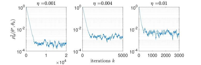
Figure 1: Paths of the algorithm in Proposition 12

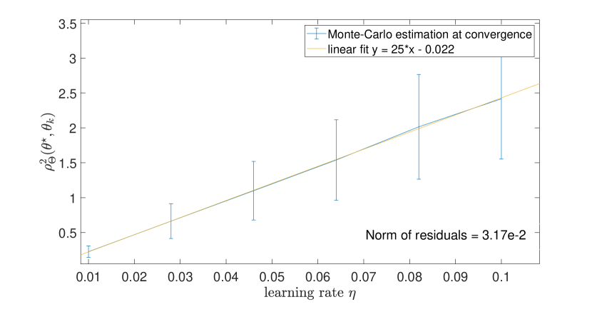
Figure 2:

Secondly, we examine the barycenter problem for $\pi=\mathbf{W}(50,\operatorname{Id})$, following the scheme introduced in (22). The estimation of ${\theta^{\star}_{\pi}}$, relative to the new distribution $\pi$, is now done with a $100$-batch-size version of our methodology, with $10^{6}$ iterations and $\upeta=10^{-4}$.

As a counterpart to Figure 1, in Figure 3 we are interested in the mean values of $(D^{2}_{\Theta}(\theta_{n},{\theta^{\star}_{\pi}}))_{n\in\mathbb{N}}$ along a single path for three step-sizes $\upeta\in\{10^{-3},4\times 10^{-3},10^{-2}\}$, with respective burn-ins $\{13,3.3,1.645\}\times 10^{3}$. As predicted by Theorem 13, an initial decrease in $\mathcal{O}(n^{-1})$ is followed by a plateau in $\mathcal{O}(\upeta)$. We can observe that compared to Figure 1, averaging smoothes oscillations.

Finally, we also perform the experiment corresponding to Figure 2 for the discrete setting to illustrate numerically that the conclusions of (7), Theorem 6 and Theorem 7 still hold. However, due to space constraints and since the conclusions are the same than for Figure 2, the corresponding figure is postponed to the supplement Figure 4.

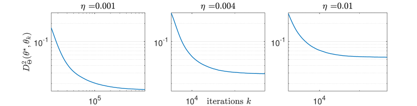
Figure 3: Paths of the algorithm in Theorem 13

Acknowledgments

AD and EM acknowledge support of the Lagrange Mathematical and Computing Research Center.

Appendix A Supplementary notation

Denote the unit tangent space $\mathrm{U}_{\theta}\Theta=\{u\in\mathrm{T}_{\theta}\Theta\,:\,\|u\|_{\theta}=1\}$. The cut-locus of $\theta$, $\mathrm{Cut}(\theta)\subset\Theta$ (Lee,, 2019, p. 308) and the injectivity domain $\mathrm{ID}(\theta)\subset\mathrm{T}_{\theta}\Theta$ (Lee,, 2019, p. 310) are two notions that inform us about the length-minimizing properties of geodesics, and therefore provide the domain of definition of the Riemannian exponential. On a complete and connected manifold, (Lee,, 2019, Theorem 10.34) holds, meaning the restriction $(\mathrm{Exp}_{\theta})_{|\mathrm{ID}(\theta)}:\mathrm{ID}(\theta)\to\Theta$ is a diffeomorphism onto its image $\Theta\setminus\mathrm{Cut}(\theta)$. We simply denote $\mathrm{Exp}_{\theta}^{-1}:\Theta\setminus\mathrm{Cut}(\theta)\to\mathrm{ID}(\theta)$ its inverse. Under the assumption that $\Theta$ is complete, simply connected and of non-positive sectional curvature, i.e. a Hadamard manifold, (Lee,, 2019, Proposition 12.9) proves that $\mathrm{Cut}(\theta)=\emptyset$ and $\mathrm{ID}(\theta)=\mathrm{T}_{\theta}\Theta$ for any $\theta\in\Theta$.

For a measure $\mu$ on a measurable space $(\mathsf{Y},\mathcal{Y})$, denote by $\mu(g)$ the integral of a measurable function $g:\mathsf{Y}\to\mathbb{R}$ with respect to $\mu$, when it exists.

Appendix B Proofs of Section 2

Under A 1 and MD 1, for any $\upeta>0$, we denote by $Q_{\upeta}$ the Markov kernel associated with $(\theta_{n})_{n\in\mathbb{N}}$ defined by (2) given for any $\mathsf{A}\in\mathcal{B}(\mathsf{S})$ and $\theta\in\mathsf{S}$ by

$$Q_{\upeta}(\theta,\mathsf{A})=\mathbb{E}\left[\mathbbm{1}_{\mathsf{A}}\left(\mathrm{Exp}_{\theta}\left\{\upeta H_{\theta}(X_{1})\right\}\right)\right]\;.$$ (24)

Useful notions, definitions and results relative to Markov chain theory are given in Section E.1.

Lemma 14.

Assume A 1, MD 1, H 1-(i)-(ii). Then for any $\upeta>0$ and $\theta_{0}\in\mathsf{S}$,

$$Q_{\upeta}V(\theta_{0})\leq V(\theta_{0})+\upeta\left\langle\mathrm{grad}\,V(\theta_{0}),h(\theta_{0})\right\rangle_{\theta_{0}}+L\upeta^{2}\left[\left\|h(\theta_{0})\right\|_{\theta_{0}}^{2}+\sigma_{0}^{2}+\sigma_{1}^{2}\left\|h(\theta_{0})\right\|_{\theta_{0}}^{2}\right]\;.$$ (25)

Proof.

Let $\theta_{0}\in\mathsf{S}$, and $\upeta>0$. Consider

$$\theta_{1/2}=\mathrm{Exp}_{\theta_{0}}\left[\upeta H_{\theta_{0}}(X_{1})\right]\;,\;\theta_{1}=\operatorname{proj}_{\mathsf{S}}\left(\theta_{1/2}\right)\;.$$ (26)

First, by definition of $Q_{\upeta}$ and H 1-(i), we have

$$Q_{\upeta}V(\theta_{0})=\mathbb{E}\left[V(\theta_{1})\right]\leq\mathbb{E}\left[V(\theta_{1/2})\right]\;.$$ (27)

Second, using A 1, H 1-(ii), (Durmus et al.,, 2020, Lemma 1) and (26), we obtain

$$V(\theta_{1/2})\leq V(\theta_{0})+\upeta\left\langle\mathrm{grad}\,V(\theta_{0}),H_{\theta_{0}}(X_{1})\right\rangle_{\theta_{0}}+(L/2)\upeta^{2}\left\|H_{\theta_{0}}(X_{1})\right\|_{\theta_{0}}^{2}\;.$$ (28)

Plugging this result in (27) and using MD 1 completes the proof of (25). ∎

B.1 Proof of Theorem 1

1. Using Lemma 14 and H 2 we have for any $\theta_{0}\in\mathsf{S}$ and $\upeta>0$,

   $$Q_{\upeta}V(\theta_{0})\leq V(\theta_{0})+\upeta\{1-C_{2}L\upeta(1+\sigma_{1}^{2})\}\left\langle\mathrm{grad}\,V(\theta_{0}),h(\theta_{0})\right\rangle_{\theta_{0}}+L\upeta^{2}[\sigma_{0}^{2}+C_{1}(1+\sigma_{1}^{2})]\;.$$ (29)

   Letting $\overline{\upeta}=[2C_{2}L(1+\sigma_{1}^{2})]^{-1}$, then for any $\upeta\in(0,\overline{\upeta}]$, we have $1-C_{2}L\upeta(1+\sigma_{1}^{2})\geq 1/2$. Therefore, using also that $\left\langle\mathrm{grad}\,V(\theta_{0}),h(\theta_{0})\right\rangle_{\theta_{0}}\leq 0$, we obtain,

   $$Q_{\upeta}V(\theta_{0})\leq V(\theta_{0})+(\upeta/2)\left\langle\mathrm{grad}\,V(\theta_{0}),h(\theta_{0})\right\rangle_{\theta_{0}}+L\upeta^{2}[\sigma_{0}^{2}+C_{1}(1+\sigma_{1}^{2})]\;.$$ (30)

   Therefore, by the Markov property, for any $k\in\mathbb{N}^{*}$, $\upeta\in(0,\overline{\upeta}]$ and $\theta_{0}\in\mathsf{S}$ we get,

   $$-(\upeta/2)\int_{\Theta}\left\langle\mathrm{grad}\,V(\theta),h(\theta)\right\rangle_{\theta}Q_{\upeta}^{k-1}(\theta_{0},\mathrm{d}\theta)\leq Q_{\upeta}^{k-1}V(\theta_{0})-Q_{\upeta}^{k}V(\theta_{0})+L\upeta^{2}[\sigma_{0}^{2}+C_{1}(1+\sigma_{1}^{2})]\;.$$ (31)

   Summing these inequalities for $k\in\{1,\dots,n\}$ concludes the proof of (a) upon using that $V$ is a non-negative function.

2. We prove (5) by using H 3$(\mathsf{K}^{\star})$ in (4) and dividing both sides by $\lambda>0$.

3. We start by using H 3$(\mathsf{K}^{\star})$ in (30). For any $\upeta\in(0,\overline{\upeta}]$ and $\theta_{0}\in\mathsf{S}$, we have

   $$Q_{\upeta}V(\theta_{0})\leq V(\theta_{0})\left[1-(\lambda\upeta/2)\mathbbm{1}_{\mathsf{S}\setminus\mathsf{K}^{\star}}(\theta_{0})\right]+\upeta^{2}b/2\;,$$ (32)

   where $b=2L[\sigma_{0}^{2}+C_{1}(1+\sigma_{1}^{2})]$. By adding and subtracting $V(\theta_{0})(\lambda\upeta/2)\mathbbm{1}_{\mathsf{K}^{\star}}(\theta_{0})$ in the right-hand side of (32), we have,

   $$Q_{\upeta}V(\theta_{0})\leq V(\theta_{0})[1-\upeta a]+\upeta(b\upeta/2+a\left\|V\right\|_{\mathsf{K}^{\star}})\;,$$ (33)

   where $a=\lambda/2$. Therefore, by a straightforward induction on $n\in\mathbb{N}$, using the Markov property, we get, for any $n\in\mathbb{N}$, $\upeta\in(0,\overline{\upeta}]$ and $\theta_{0}\in\mathsf{S}$,

   $$\mathbb{E}\left[V(\theta_{n})\right] \leq\{1-\upeta a\}^{n}V(\theta_{0})+\upeta(b\upeta/2+a\left\|V\right\|_{\mathsf{K}^{\star}})\sum_{k=0}^{n-1}[1-\upeta a]^{k}$$ (34)

   $$\leq\{1-\upeta a\}^{n}V(\theta_{0})+\{\left\|V\right\|_{\mathsf{K}^{\star}}+(b\upeta/2a)\}\;,$$ (35)

   which concludes the proof of (c) and Theorem 1.

B.2 An alternative to Theorem 1-(b)

Consider the following condition for some compact set $\mathsf{K}^{\star}\subset\mathsf{S}$.

HS 1 ($\mathsf{K}^{\star}$).

There exists $\lambda>0$ such that for any $\theta\in\mathsf{S}$, $\left\langle\mathrm{grad}\,V(\theta),h(\theta)\right\rangle_{\theta}\leq-\lambda\left\|h(\theta)\right\|_{\theta}^{2}\mathbbm{1}_{\mathsf{S}\setminus\mathsf{K}^{\star}}(\theta)$.

Theorem 15.

Assume A 1, MD 1, H 1-(i)-(ii) and HS 1$(\mathsf{K}^{\star})$ hold for some compact set $\mathsf{K}^{\star}\subset\mathsf{S}$, and define $\left\|h\right\|_{\mathsf{K}^{\star}}=\sup\{\left\|h(\theta)\right\|_{\theta}\,:\,\theta\in\mathsf{K}^{\star}\}$ if $\mathsf{K}^{\star}\neq\emptyset$ and $\left\|h\right\|_{\mathsf{K}^{\star}}=0$ otherwise. Then for any $\upeta\in\left(0,\check{\upeta}\right]$ and $\theta_{0}\in\mathsf{S}$, and $n\in\mathbb{N}^{*}$,

$$n^{-1}\sum_{k=0}^{n-1}\mathbb{E}[\mathbbm{1}_{\mathsf{S}\setminus\mathsf{K}^{\star}}(\theta_{k})\left\|h(\theta_{k})\right\|_{\theta_{k}}^{2}]\leq V(\theta_{0})/(an\upeta)+\upeta\tilde{b}/a\;,$$ (36)

where $(\theta_{n})_{n\in\mathbb{N}}$ is defined by (2) starting from $\theta_{0}$, $\check{\upeta}=\lambda/[2(1+\sigma^{2}_{1})L]$, $a=\lambda/2$ and $\tilde{b}=L((1+\sigma_{1}^{2})\left\|h\right\|_{\mathsf{K}^{\star}}+\sigma_{0}^{2})$.

Proof.

By Lemma 14 and HS 1$(\mathsf{K}^{\star})$, for any $\upeta\in(0,\overline{\upeta}]$ and $\theta_{0}\in\mathsf{S}$, we have

$$Q_{\upeta}V(\theta_{0})\leq V(\theta_{0})-\upeta\lambda\left\|h(\theta_{0})\right\|_{\theta_{0}}^{2}\mathbbm{1}_{\mathsf{S}\setminus\mathsf{K}^{\star}}(\theta_{0})+L\upeta^{2}\left[\left\|h(\theta_{0})\right\|_{\theta_{0}}^{2}+\sigma_{0}^{2}+\sigma_{1}^{2}\left\|h(\theta_{0})\right\|_{\theta_{0}}^{2}\right]\;.$$ (37)

Therefore, by the Markov property, for any $k\in\mathbb{N}^{*}$, $\upeta\in(0,\overline{\upeta}]$ and $\theta_{0}\in\mathsf{S}$, we get

$$(\upeta\lambda/2)\int_{\Theta}\{\mathbbm{1}_{\mathsf{S}\setminus\mathsf{K}^{\star}}(\theta)\left\|h(\theta)\right\|_{\theta}^{2}\}Q_{\upeta}^{k-1}(\theta_{0},\mathrm{d}\theta)\\ \leq Q_{\upeta}^{k-1}V(\theta_{0})-Q_{\upeta}^{k}V(\theta_{0})+L\upeta^{2}((1+\sigma_{1}^{2})\left\|h\right\|_{\mathsf{K}^{\star}}+\sigma_{0}^{2})\;.$$ (38)

Summing these inequalities for $k\in\{1,\ldots,n\}$ concludes the proof upon using that $V$ is a non-negative function. ∎

B.3 Proof of Theorem 2

Lemma 16.

Assume A 1, MD 1 and MD 2-(i). Then the Markov kernel $Q_{\upeta}$ on $\mathsf{S}\times\mathcal{B}(\mathsf{S})$ is Feller, i.e.  for any measurable bounded function $f:\mathsf{S}\to\mathbb{R}$, $Q_{\upeta}f$ is continuous from $\mathsf{S}$ to $\mathbb{R}$.

Proof.

The proof is an easy consequence of the Lebesgue dominated convergence theorem, since $h$ is continuous and MD 2-(i) holds. ∎

For the next lemma, we introduce $\mu_{\mathsf{S}}$, the restriction to $\mathsf{S}$ of the Riemannian measure $\mu_{\Theta}$ associated with the volume form on $\Theta$.

Lemma 17.

Assume A 1, MD 1 and MD 2-(ii). Then $Q_{\upeta}$ is $\mu_{\mathsf{S}}$-irreducible and aperiodic.

Proof.

We consider first the case A 1-(i), where $\Theta$ is a Hadamard manifold. Let $\mathsf{A}\in\mathcal{B}(\mathsf{S})$ be a Borel set of $\mathsf{S}$, such that $\mu_{\mathsf{S}}(\mathsf{A})>0$. We only need to show that for any $\theta_{0}\in\Theta$, $Q_{\upeta}(\theta_{0},\mathsf{A})>0$. Indeed, this gives $\mu_{\mathsf{S}}$-irreducibility by definition and implies that the chain is aperiodic by (Meyn and Tweedie,, 2009, Theorem 5.4.4) since for any $\mathsf{A}\in\mathcal{B}(\mathsf{S})$, $\mu_{\mathsf{S}}(\mathsf{A})>0$, $\theta\in\mathsf{A}$, we have $Q_{\upeta}(\theta,\mathsf{A})>0$.

Let $\theta_{0}\in\mathsf{S}$. By definition of the scheme (2) and $\operatorname{proj}_{\mathsf{S}}$, $Q_{\upeta}(\theta_{0},\mathsf{A})=\mathbb{P}(\operatorname{proj}_{\mathsf{S}}\circ\mathrm{Exp}_{\theta_{0}}(\upeta\{h(\theta_{0})+e_{\theta_{0}}(X_{1})\})\in\mathsf{A})\geq\mathbb{P}(\mathrm{Exp}_{\theta_{0}}(\upeta\{h(\theta_{0})+e_{\theta_{0}}(X_{1})\})\in\mathsf{A})$. However, using MD 2-(ii), the law of $e_{\theta_{0}}(X_{1})$ has a positive density $\phi:\mathrm{T}_{\theta_{0}}\Theta\to(0,+\infty)$ with respect to Lebesgue’s measure $\mathrm{Leb}_{\theta_{0}}$. Denote $(\mathfrak{g}_{ij}(\theta))_{1\leq i,j\leq d}$ the matrix representing the Riemannian metric at $\theta\in\Theta$ in normal global coordinates at $\theta_{0}$. Expressing $\mu_{\mathsf{S}}$ in these coordinates and using (Lee,, 2019, p.404 and Proposition 2.41),

$$\mathbb{P}(\upeta\{h(\theta_{0})+e_{\theta_{0}}(X_{1})\}\in\mathrm{Exp}_{\theta_{0}}^{-1}(\mathsf{A}))=\int_{\mathrm{Exp}^{-1}_{\theta_{0}}(\mathsf{A})}\phi\left(\upeta^{-1}v-h(\theta_{0})\right)\mathrm{d}\mathrm{Leb}_{\theta_{0}}(v)$$ (39)

$$\qquad\qquad\qquad=\int_{\mathsf{A}}\phi\left(\upeta^{-1}\mathrm{Exp}^{-1}_{\theta_{0}}(\theta)-h(\theta_{0})\right)\left\{\det(\mathfrak{g}_{ij}(\theta))\right\}^{-1/2}\mathrm{d}\mu_{\mathsf{S}}(\theta)>0\;,$$ (40)

since all quantities in the integral are positive and $\mu_{\mathsf{S}}(\mathsf{A})>0$.

Now assume A 1-(ii) and keep the notations of the first case. Then $\mathrm{Exp}_{\theta_{0}}:\mathrm{T}_{\theta_{0}}\Theta\to\Theta$ is no longer a diffeomorphism. However, $(\mathrm{Exp}_{\theta_{0}})_{|\mathrm{ID}(\theta_{0})}:\mathrm{ID}(\theta_{0})\to\Theta\setminus\mathrm{Cut}(\theta_{0})$ is a diffeomorphism, see (Lee,, 2019, Theorem 10.34). Moreover, as $\mathrm{Cut}(\theta_{0})$ is a set of measure zero, see again (Lee,, 2019, Theorem 10.34), considering $\tilde{\mathsf{A}}=\mathsf{A}\setminus\mathrm{Cut}(\theta_{0})$ allows the previous proof to give the desired result. ∎

Proof of Theorem 2.

First, we prove that the chain is Harris-recurrent. For that, we start by proving, for any $\theta_{0}\in\mathsf{S}$,

$$\mathbb{P}\left(\cup_{k\in\mathbb{N}^{*}}\cap_{N\in\mathbb{N}}\cup_{n\geq N}\{\theta_{n}\in\overline{\mathrm{B}}(\theta^{\star},k)\}\right)=1\;,$$ (41)

where $(\theta_{n})_{n\in\mathbb{N}}$ is defined by (2) and with initial condition $\theta_{0}$.

Theorem 1-(6) implies that for any $\theta_{0}\in\Theta$, $\sup_{n\in\mathbb{N}}Q^{n}_{\upeta}V(\theta_{0})<+\infty$; since $\left\|V\right\|_{\mathsf{K}^{\star}}=\sup_{\mathsf{K}^{\star}}V<+\infty$ because $V$ is assumed to be continuous. Therefore $\liminf_{n\to+\infty}V(\theta_{n})$ is integrable by Fatou’s lemma. Thus, for any $k\in\mathbb{N}^{*}$, using Markov’s inequality,

$$\mathbb{P}\left(\liminf_{n\to+\infty}V(\theta_{n})>k\right)\leq\left.\mathbb{E}\left[\liminf_{n\to+\infty}V(\theta_{n})\right]\middle/k\right.\;.$$ (42)

However, $\{\liminf_{n\to+\infty}V(\theta_{n})\leq k\}=\cap_{N\in\mathbb{N}}\cup_{n\geq N}\{\theta_{n}\in V^{-1}([0,k])\}$. Thus, for any $k\in\mathbb{N}^{*}$,

$$\mathbb{P}\left(\cap_{N\in\mathbb{N}}\cup_{n\geq N}\left\{\theta_{n}\in V^{-1}([0,k])\right\}\right)\geq 1-\left.\mathbb{E}\left[\liminf_{n\to+\infty}V(\theta_{n})\right]\middle/k\right.\;.$$ (43)

Now, taking the union of these events for any $k\in\mathbb{N}^{*}$ gives

$$\mathbb{P}\left(\cup_{k\in\mathbb{N}^{*}}\cap_{N\in\mathbb{N}}\cup_{n\geq N}\left\{\theta_{n}\in V^{-1}([0,k])\right\}\right)=1\;.$$ (44)

Nonetheless, using H 1-(iii), for any $k\in\mathbb{N}^{*}$, $V^{-1}([0,k])$ is a subset of a compact set, therefore it is bounded. Thus, for any $k\in\mathbb{N}^{*}$, there exists $k^{\prime}\in\mathbb{N}^{*}$ such that $V^{-1}([0,k])\subset\overline{\mathrm{B}}(\theta^{\star},k^{\prime})$. This gives the following,

$$\cup_{k\in\mathbb{N}^{*}}\cap_{N\in\mathbb{N}}\cup_{n\geq N}\left\{\theta_{n}\in V^{-1}([0,k])\right\}\subset\cup_{k\in\mathbb{N}^{*}}\cap_{N\in\mathbb{N}}\cup_{n\geq N}\left\{\theta_{n}\in\overline{\mathrm{B}}(\theta^{\star},k)\right\}\;.$$ (45)

Combining this with (44) gives (41).

Equation 41 gives that the chain is non-evanescent (Meyn and Tweedie,, 2009, Section 9.2.1). Since $Q_{\upeta}$ is Feller (see Lemma 16), this result and (Meyn and Tweedie,, 2009, Theorem 9.2.2) imply that $Q_{\upeta}$ is Harris recurrent.

We now show that $Q_{\upeta}$ is $\tilde{V}$-uniformly geometrically ergodic (see Section E.1) setting $\tilde{V}=1+V$. First, by Theorem 1 and (33) obtained in the proof above, we have that for any $\theta_{0}\in\mathsf{S},\upeta\in(0,\overline{\upeta}]$,

$$Q_{\upeta}\tilde{V}(\theta_{0})\leq(1-\upeta a)\tilde{V}(\theta_{0})+\upeta(\upeta b/2+a(1+\left\|V\right\|_{\mathsf{K}^{\star}}))\;,$$ (46)

where $a,b,\overline{\upeta}$ and $\left\|V\right\|_{\mathsf{K}^{\star}}$ are defined in Theorem 1. Then, by H 1-(iii) there exists $\tilde{r}>0$, such that for any $\theta_{0}\in\mathsf{S}$,

$$Q_{\upeta}\tilde{V}(\theta_{0})\leq(1-a\upeta/2)\tilde{V}(\theta_{0})+\upeta(\upeta b/2+a(1+\left\|V\right\|_{\mathsf{K}^{\star}}))\mathbbm{1}_{\overline{\mathrm{B}}(\theta^{\star},\tilde{r})}(\theta_{0})\;.$$ (47)

Then, since $Q_{\upeta}$ is Feller by Lemma 16 and $\mu_{\mathsf{S}}$-irreducible by Lemma 17, using (Meyn and Tweedie,, 2009, Proposition 6.2.8 (ii)), $\overline{\mathrm{B}}(\theta^{\star},r)$ is petite since it is compact by the Hopf-Rinow theorem (Jost,, 2005, Theorem 1.7.1) and $\mathsf{S}$ has non-empty interior by A 1. Therefore, an application of (Meyn and Tweedie,, 2009, Theorem 16.0.1) proves that the chain is $\tilde{V}$-uniformly geometrically ergodic. ∎

B.4 Proof of Theorem 3

Lemma 18.

Assume A 1, MD 1 MD 2, H 1, H 2 and H 3$(\mathsf{K}^{\star})$ hold for some compact set $\mathsf{K}^{\star}\subset\mathsf{S}$. Then for any $\upeta\in(0,\overline{\upeta}]$,

$$\mu^{\upeta}[V\mathbbm{1}_{\mathsf{S}\setminus\mathsf{K}^{\star}}]\leq 2\upeta L\{\sigma_{0}^{2}+C_{1}(1+\sigma_{1}^{2})\}/\lambda\;,$$ (48)

where $\overline{\upeta}=[2C_{2}L(1+\sigma_{1}^{2})]^{-1}$.

Proof.

For any $\upeta\in(0,\overline{\upeta}]$ and $M\geq 0$, setting $V_{M}=M\wedge V$, (32) implies using Jensen inequality, for any $\theta_{0}\in\Theta$,

$$Q_{\upeta}V_{M}\left(\theta_{0}\right)\leq(1-\upeta a\mathbbm{1}_{\mathsf{S}\setminus\mathsf{K}^{\star}}(\theta_{0}))V_{M}\left(\theta_{0}\right)+\upeta^{2}b/2\;,$$ (49)

where $\overline{\upeta}=[2C_{2}L(1+\sigma_{1}^{2})]^{-1}$ , $b=2L\{\sigma_{0}^{2}+C_{1}(1+\sigma_{1}^{2})\}$ and $a=\lambda/2$. Using that $\mu^{\upeta}$ is invariant for $Q_{\upeta}$ by Theorem 2 and $V_{M}$ is bounded, we get $\mu^{\upeta}[V_{M}\mathbbm{1}_{\mathsf{S}\setminus\mathsf{K}^{\star}}]\leq\upeta b/(2a)$. By the monotone convergence theorem, taking $M\to+\infty$, we have $\mu^{\upeta}[V\mathbbm{1}_{\mathsf{S}\setminus\mathsf{K}^{\star}}]\leq\upeta b/(2a)$, which concludes the proof. ∎

Proof of Theorem 3.

1. Using Lemma 18 and $V(\theta)\geq c>0$ for any $\theta\in\mathsf{S}\setminus\mathsf{K}^{\star}$, we obtain

   $$\mu^{\upeta}\left\{\mathsf{S}\setminus\mathsf{K}^{\star}\right\}\leq\upeta b/(2ac)\;,$$ (50)

   which concludes the proof of (a) taking the limit $\upeta\to 0$.

2. Let $(\upeta_{n})_{n\in\mathbb{N}}$ be a sequence converging to zero such that for any $n\in\mathbb{N}$, $\upeta_{n}\in(0,\overline{\upeta}]$. We start by proving that $(\mu^{\upeta_{n}})_{n\in\mathbb{N}}$ is tight. Let $\varepsilon>0$. On one hand, let $r>0$ and $\mathsf{K}_{0}=\overline{\mathrm{B}}(\theta^{\star},r)$. Then, using Theorem 3-(a), there exists $N\in\mathbb{N}$ such that for any $n\geq N$, $\mu^{\upeta_{n}}(\mathsf{K}_{0})\geq 1-\varepsilon$. On the other hand, $(\mu^{\upeta_{n}})_{n\in\{0,\dots,N-1\}}$ is tight, i.e. there exists a compact set $\tilde{\mathsf{K}}\subset\Theta$ such that for any $n\in\{1,\dots,N-1\}$, $\mu^{\upeta_{n}}(\tilde{\mathsf{K}})\geq 1-\varepsilon$. Finally, taking $\mathsf{K}=\mathsf{K}_{0}\cup\tilde{\mathsf{K}}$ gives the tightness of $(\mu^{\upeta_{n}})_{n\in\mathbb{N}}$. Now, let $\mu$ be a limit point of $(\mu^{\upeta_{n}})_{n\in\mathbb{N}}$. Using Theorem 3-(a), and Lebesgue’s dominated convergence theorem letting $r\to 0$, gives $\mu(\{\theta^{\star}\})=1$, i.e. $\mu=\updelta_{\theta^{\star}}$. In conclusion, for any $(\upeta_{n})_{n\in\mathbb{N}}$ converging to zero, $(\mu^{\upeta_{n}})_{n\in\mathbb{N}}$ converges weakly to the Dirac at $\theta^{\star}$.

∎

B.5 Proof of Proposition 4

First, we check H 1-(i). Using (Sturm,, 2003, Proposition 2.6), $\operatorname{proj}_{\mathsf{S}}$ is a contraction w.r.t. $\rho_{\Theta}$, which implies that for any $\theta\in\Theta$,

$$\rho_{\Theta}^{2}(\theta^{\star},\operatorname{proj}_{\mathsf{S}}(\theta))=\rho_{\Theta}^{2}(\operatorname{proj}_{\mathsf{S}}(\theta^{\star}),\operatorname{proj}_{\mathsf{S}}(\theta))\leq\rho_{\Theta}^{2}(\theta^{\star},\theta)\;.$$ (51)

This implies, since $\mathsf{S}\subset\mathsf{H}$, that

$$V_{2}(\operatorname{proj}_{\mathsf{S}}(\theta))=\rho_{\Theta}^{2}(\theta^{\star},\operatorname{proj}_{\mathsf{S}}(\theta))\leq\chi_{\mathsf{H}}(\theta)\rho_{\Theta}^{2}(\theta^{\star},\theta)+(1-\chi_{\mathsf{H}}(\theta))\operatorname{diam}^{2}(\overline{\mathsf{H}})=V_{2}(\theta)\;,$$ (52)

which gives H 1-(i).

To prove H 1-(ii), we calculate the operator norm of the Hessian of $V_{2}$ and conclude by (Durmus et al.,, 2020, Lemma 10). Using A 2 and (Jost,, 2005, Theorem 5.6.1), $\theta\mapsto\rho_{\Theta}^{2}({\theta^{\star}},\theta)$ is smooth and its gradient on $\Theta$ is given by $\theta\mapsto-2\mathrm{Exp}^{-1}_{\theta}(\theta^{\star})$. Therefore, for any $\theta\in\Theta$,

$$\mathrm{grad}\,V_{2}(\theta)=[\rho_{\Theta}^{2}({\theta^{\star}},\theta)-\mathrm{D}_{\mathsf{H}}^{2}]\mathrm{grad}\,\chi_{\mathsf{H}}(\theta)-2\chi_{\mathsf{H}}(\theta)\mathrm{Exp}_{\theta}^{-1}({\theta^{\star}})\;.$$ (53)

Using now A 2, (Jost,, 2005, Theorem 5.6.1) and Cauchy-Schwarz’s inequality brings, for any $\theta\in\Theta,v\in\mathrm{T}_{\theta}\Theta$,

$$\left\|(\mathrm{Hess}\,V_{2})_{\theta}(v,v)\right\|_{\theta} \leq 2\kappa\rho_{\Theta}({\theta^{\star}},\theta)\coth(\kappa\rho_{\Theta}({\theta^{\star}},\theta))\chi_{\mathsf{H}}(\theta)\left\|v\right\|_{\theta}^{2}+4\rho_{\Theta}({\theta^{\star}},\theta)\left\|\mathrm{grad}\,\chi_{\mathsf{H}}(\theta)\right\|_{\theta}\left\|v\right\|_{\theta}^{2}$$ (54)

$$\quad+\left\|(\mathrm{Hess}\,\chi_{\mathsf{H}})_{\theta}(v,v)\right\|_{\theta}\left|\rho_{\Theta}^{2}({\theta^{\star}},\theta)-\mathrm{D}_{\mathsf{H}}^{2}\right|\;.$$ (55)

However, one can choose $\chi_{\mathsf{H}}$ such that for any $\theta\in\Theta$ satisfying $\inf_{\theta^{\prime}\in\mathsf{H}}\rho_{\Theta}(\theta^{\prime},\theta)\geq 1$, it holds that $\chi_{\mathsf{H}}(\theta)=0$. Therefore, for any $\theta\in\Theta$, $\rho_{\Theta}({\theta^{\star}},\theta)\chi_{\mathsf{H}}(\theta)\leq\mathrm{D}_{\mathsf{H}}+1$. Since $\chi_{\mathsf{H}}$ is smooth with compact support, there exists a constant $M>0$ such that for any $\theta\in\Theta$ and $v\in\mathrm{T}_{\theta}\Theta$,

$$\|\mathrm{grad}\,\chi_{\mathsf{H}}(\theta)\|_{\theta}\leq M\quad\text{ and }\quad\|(\mathrm{Hess}\,\chi_{\mathsf{H}})_{\theta}(v,v)\|_{\theta}\leq M\left\|v\right\|_{\theta}^{2}\;.$$ (56)

Therefore, combining these expressions brings for any $\theta\in\Theta$ and $v\in\mathrm{T}_{\theta}\Theta$,

$$\left\|(\mathrm{Hess}\,V_{2})_{\theta}(v,v)\right\|_{\theta}\leq 6(M+1)(\mathrm{D}_{\mathsf{H}}+1)[1+\kappa\coth(\kappa\mathrm{D}_{\mathsf{H}})]\left\|v\right\|_{\theta}^{2}\;,$$ (57)

thus proving by (Durmus et al.,, 2020, Lemma 10) and setting $C_{\chi}=6(M+1)$, that H 1-(ii) holds with $L\leftarrow C_{\chi}(1+\mathrm{D}_{\mathsf{H}})[1+\kappa\coth(\kappa\mathrm{D}_{\mathsf{H}})]$.

We now turn on checking H 3$(\overline{\operatorname{B}}({\theta^{\star}},r))$. Since $\mathrm{grad}\,\chi_{\mathsf{H}}(\theta)=0$ for any $\theta\in\mathsf{S}$, we get that $V_{2}$ is smooth and for any $\theta\in\mathsf{S},\mathrm{grad}\,V_{2}(\theta)=-2\mathrm{Exp}^{-1}_{\theta}(\theta^{\star})$ Therefore H 3$(\overline{\operatorname{B}}({\theta^{\star}},r))$ holds by (9).

B.6 Proof of Proposition 5

First, we check H 1-(i). Using (Sturm,, 2003, Proposition 2.6), $\operatorname{proj}_{\mathsf{S}}$ is a contraction w.r.t. $\rho_{\Theta}$, which implies that $\theta\in\Theta$,

$$\rho_{\Theta}(\theta^{\star},\operatorname{proj}_{\mathsf{S}}(\theta))=\rho_{\Theta}(\operatorname{proj}_{\mathsf{S}}(\theta^{\star}),\operatorname{proj}_{\mathsf{S}}(\theta))\leq\rho_{\Theta}(\theta^{\star},\theta)\;.$$ (58)

Then the proof of H 1-(i) is completed using that $x\mapsto\delta^{2}\{(x/\delta)^{2}+1\}^{1/2}-\delta^{2}$ is increasing.

Next, using A 2, (Durmus et al.,, 2020, Lemma 16), we have for any $\theta\in\Theta,v\in\mathrm{T}_{\theta}\Theta\setminus\{0\}$,

$$0<\mathrm{Hess}\,V_{1}(\theta)(v,v)\leq(1+\kappa\delta)\left\|v\right\|_{\theta}^{2}\;.$$ (59)

Therefore, using (Durmus et al.,, 2020, Lemma 10), H 1-(ii) holds for $L=1+\kappa\delta$. It is easy to see that as $\rho_{\Theta}({\theta^{\star}},\theta)\to\infty$, $V_{1}(\theta)\to+\infty$, meaning H 1-(iii) holds by the Hopf-Rinow theorem (Jost,, 2005, Theorem 1.7.1).

Regarding H 3$(\overline{\operatorname{B}}({\theta^{\star}},r))$, using (Durmus et al.,, 2020, Lemma 16), we have for any $\theta\in\Theta$,

$$\mathrm{grad}\,V_{1}(\theta)=-\left.{\mathrm{Exp}^{-1}_{\theta}(\theta^{\star})}\middle/\left\{\left(\rho_{\Theta}(\theta^{\star},\theta)/\delta\right)^{2}+1\right\}^{1/2}\right.\;,$$ (60)

Therefore for any $\theta\in\Theta$, we get

$$\left\langle\mathrm{grad}\,V_{1}(\theta),h(\theta)\right\rangle_{\theta} =-\left.\left\langle\mathrm{Exp}^{-1}_{\theta}(\theta^{\star}),h(\theta)\right\rangle_{\theta}\middle/\left\{\left(\rho_{\Theta}(\theta^{\star},\theta)/\delta\right)^{2}+1\right\}^{1/2}\right.\;.$$ (61)

Then, under the condition (9), we obtain

$$\left\langle\mathrm{grad}\,V_{1}(\theta),h(\theta)\right\rangle_{\theta} \leq\left.-\lambda_{\rho}\rho_{\Theta}^{2}(\theta^{\star},\theta)\mathbbm{1}_{\mathsf{S}\setminus\overline{\operatorname{B}}(\theta^{\star},r)}(\theta)\middle/\left\{\left(\rho_{\Theta}(\theta^{\star},\theta)\middle/\delta\right)^{2}+1\right\}^{1/2}\right.$$ (62)

$$\leq-\lambda_{\rho}V_{1}(\theta)\mathbbm{1}_{\mathsf{S}\setminus\overline{\operatorname{B}}(\theta^{\star},r)}(\theta)\;,$$

where we used that

$$V_{1}(\theta)\leq\left.{\rho_{\Theta}^{2}(\theta^{\star},\theta)}\middle/\left\{\left(\rho_{\Theta}(\theta^{\star},\theta)/\delta\right)^{2}+1\right\}^{1/2}\right.\;,$$ (63)

since for any $a>0$ and $x\geq 0$, $(ax^{2}+1)^{1/2}-1=a\int_{0}^{x}t\{at^{2}+1\}^{-1/2}\mathrm{d}t\leq ax^{2}/\{ax^{2}+1\}^{1/2}$.

Appendix C Proofs of Section 3

For any $K\in\mathbb{R}_{+}$, consider a smooth function with compact support $\chi_{K}:\mathbb{R}_{+}\to[0,1]$ such that $\chi_{K}(t)=1$ for any $t\leq K$ and $\chi_{K}(t)=0$ for any $t\geq K+1$.

Lemma 19.

Assume A 1-(ii) and MD 1.

1. Then, for any smooth function with compact support $g:\Theta\to\mathbb{R}$, any $\upeta>0$ and $\theta_{0}\in\Theta$,

   $$Q_{\upeta}g(\theta_{0})=g(\theta_{0})+\upeta\left\langle\mathrm{grad}\,g(\theta_{0}),h(\theta_{0})\right\rangle_{\theta_{0}}+(\upeta^{2}/2)\left[\mathrm{Hess}\,g:\Sigma+h\otimes h\right](\theta_{0})+(\upeta^{2}/6)\mathscr{R}_{g,\upeta}(\theta_{0})\;,$$ (64)

   where for any $K>0$,

   $$\left|\mathscr{R}_{g,\upeta}(\theta_{0})\right|\leq 8\upeta\mathbb{E}\left[\|\nabla\mathrm{Hess}\,g\|_{\upgamma,\infty}\mathbbm{1}_{\mathsf{A}_{\theta_{0}}^{\complement}}\left\|H_{K}\right\|_{\theta_{0}}^{3}\right]+16\|\mathrm{Hess}\,g\|_{\infty}\mathbb{E}\left[\left\|Y_{K}\right\|_{\theta_{0}}^{2}\right]\;,$$ (65)

   $$H_{K}=h(\theta_{0})+e_{\theta_{0}}(X_{1})\chi_{K}(\|e_{\theta_{0}}(X_{1})\|_{\theta_{0}})\;,\quad Y_{K}=e_{\theta_{0}}(X_{1})\{1-\chi_{K}(\|e_{\theta_{0}}(X_{1})\|_{\theta_{0}})\}\;,\qquad$$ (66)

   $$\|\mathrm{Hess}\,g\|_{\infty}=\sup\{|\mathrm{Hess}\,g_{\theta}(u,u)|\,:\,\theta\in\Theta,u\in\mathrm{U}_{\theta}\Theta\}\;,$$ (67)

   $$\|\nabla\mathrm{Hess}\,g\|_{\upgamma,\infty}=\sup\{|\nabla\mathrm{Hess}\,g_{\upgamma(t)}(u,u,u)|\,:\,t\in[0,1],u\in\mathrm{U}_{\upgamma(t)}\Theta\}\;,$$ (68)

   $\mathsf{A}_{\theta_{0}}=\{\|H_{K}\|_{\theta_{0}}\leq\|Y_{K}\|_{\theta_{0}}\}$ and $\upgamma:[0,1]\to\Theta$ is defined for any $t\in\left[0,1\right]$ by $\upgamma(t)=\mathrm{Exp}_{\theta_{0}}(t\upeta H_{\theta_{0}}(X_{1}))$.

2. Assume in addition that there exist $C_{3}>0$ and ${\theta^{\star}}\in\Theta$ such that for any $\theta\in\Theta$, $\|h(\theta)\|_{\theta}\leq C_{3}\rho_{\Theta}({\theta^{\star}},\theta)$. Then, for any smooth function with compact support $g:\Theta\to\mathbb{R}$, any $\upeta\in(0,(4C_{3})^{-1}]$ and $\theta_{0}\in\Theta$, (64) holds, with for any $K>0$,

   $$\left|\mathscr{R}_{g,\upeta}(\theta_{0})\right|\leq 8\upeta\mathbbm{1}_{\mathsf{K}_{K}}(\theta_{0})\mathbb{E}\left[\|\nabla\mathrm{Hess}\,g\|_{\upgamma,\infty}\mathbbm{1}_{\mathsf{A}_{\theta_{0}}^{\complement}}\left\|H_{K}\right\|_{\theta_{0}}^{3}\right]+16\|\mathrm{Hess}\,g\|_{\infty}\mathbb{E}\left[\left\|Y_{K}\right\|_{\theta_{0}}^{2}\right]\;,$$ (69)

   where we take the notation of (a) and $\mathsf{K}_{K}$ is a compact subset of $\Theta$.

Proof.

1. Let $g:\Theta\to\mathbb{R}$ be a smooth function with compact support and $\theta_{0}\in\Theta$. Using (2), A 1-(ii) and the definition of $Q_{\upeta}$ (24), we have

   $$Q_{\upeta}g({\theta_{0}})=\mathbb{E}\left[g\left\{\mathrm{Exp}_{\theta_{0}}[\upeta H_{\theta_{0}}(X_{1})]\right\}\right]\;.$$ (70)

   Consider the geodesic $\upgamma:[0,1]\to\Theta$ defined for any $t\in\left[0,1\right]$ by $\upgamma(t)=\mathrm{Exp}_{\theta_{0}}(t\upeta H_{\theta_{0}}(X_{1}))$. For any $t\in[0,1]$, let $\mathpzc{g}(t)=(g\circ\upgamma)(t)$. We compute now its derivatives to derive a Taylor expansion. Using (Lee,, 2019, Proposition 4.15-(ii) and Theorem 4.24-(iii)), we have for any $t\in[0,1]$,

   $$\mathpzc{g}^{\prime}(t)=\mathrm{D}_{t}(g\circ\upgamma)(t)=\langle\mathrm{grad}\,g(\upgamma(t)),\dot{\upgamma}(t)\rangle_{\upgamma(t)}\;.$$ (71)

   By definition of the Hessian (Lee,, 2019, Example 4.22) and using $\mathrm{D}_{t}\dot{\upgamma}(t)=0$, Proposition 27-(207)-(iv), we get for any $t\in[0,1]$,

   $$\mathpzc{g}^{\prime\prime}(t)=[\mathrm{D}^{2}_{t}\mathpzc{g}](t)=\mathrm{Hess}\,g_{\upgamma(t)}(\dot{\upgamma}(t),\dot{\upgamma}(t))\;,$$ (72)

   In addition, using $\mathrm{D}_{t}\dot{\upgamma}(t)=0$ and Proposition 27-(207)-(iv), we obtain for any $t\in[0,1]$,

   $$\mathpzc{g}^{(3)}(t)=[\mathrm{D}^{3}_{t}\mathpzc{g}](t)=\nabla\mathrm{Hess}\,g_{\upgamma(t)}(\dot{\upgamma}(t),\dot{\upgamma}(t),\dot{\upgamma}(t))\;,$$ (73)

   where $\nabla\mathrm{Hess}\,g$ is the total covariant derivative of $\mathrm{Hess}\,g$ (Lee,, 2019, Proposition 4.17). Finally, for any $K>0$, consider the two random tangent vectors at ${\theta_{0}}$ defined in (66). Now, writing the first-order Taylor expansion of $\mathpzc{g}:[0,1]\to\mathbb{R}$, at $t=1$ on the event $\mathsf{A}_{\theta_{0}}=\{\|H_{K}\|_{\theta_{0}}\leq\|Y_{K}\|_{\theta_{0}}\}$, the second-order one on the complement, and summing both expansions, we get

   $$g\left(\mathrm{Exp}_{\theta_{0}}(\upeta H_{\theta_{0}}(X_{1}))\right) =g({\theta_{0}})+\upeta\langle\mathrm{grad}\,g({\theta_{0}}),H_{\theta_{0}}(X_{1})\rangle_{\theta_{0}}$$ (74)

   $$\quad+(\upeta^{2}/2)\mathrm{Hess}\,g_{\theta_{0}}(H_{\theta_{0}}(X_{1}),H_{\theta_{0}}(X_{1}))+\mathscr{R}_{g,\upeta}({\theta_{0}},X_{1})/6\;,$$

   where the remainder term is given by

   $$\mathscr{R}_{g,\upeta}({\theta_{0}},X_{1}) =\mathbbm{1}_{\mathsf{A}_{\theta_{0}}^{\complement}}\int_{0}^{1}\nabla\mathrm{Hess}\,g_{\upgamma(t)}(\dot{\upgamma}(t),\dot{\upgamma}(t),\dot{\upgamma}(t))\mathrm{d}t$$ (75)

   $$\quad+\mathbbm{1}_{\mathsf{A}_{\theta_{0}}}\left[\int_{0}^{1}\mathrm{Hess}\,g_{\upgamma(t)}(\dot{\upgamma}(t),\dot{\upgamma}(t))\mathrm{d}t-3\upeta^{2}\mathrm{Hess}\,g_{{\theta_{0}}}(H_{{\theta_{0}}}(X_{1}),H_{{\theta_{0}}}(X_{1}))\right]\;.$$

   We bound the remainder as follows. Since $g$ has compact support, $\mathrm{Hess}\,g$ and $\nabla\mathrm{Hess}\,g$ have an operator norm uniformly bounded over $\Theta$, which we express in the following way. For any $\theta\in\Theta$, consider the unit tangent space at $\theta$, $\mathrm{U}_{\theta}\Theta=\{v\in\mathrm{T}_{\theta}\Theta\,:\,\|v\|_{\theta}=1\}$, let $\|\mathrm{Hess}\,g\|_{\infty}=\sup\{|\mathrm{Hess}\,g_{\theta}(v,v)|\,:\,\theta\in\Theta,v\in\mathrm{U}_{\theta}\Theta\}$ and $\|\nabla\mathrm{Hess}\,g\|_{\upgamma,\infty}=\sup\{|\nabla\mathrm{Hess}\,g_{\upgamma(t)}(v,v,v)|\,:\,t\in[0,1],v\in\mathrm{U}_{\upgamma(t)}\Theta\}$. Then, using (Lee,, 2019, Corollary 5.6-$(b)$), and $\dot{\upgamma}(0)=\upeta H_{\theta_{0}}(X_{1})$,

   $$\left|\mathscr{R}_{g,\upeta}({\theta_{0}},X_{1})\right| \leq\mathbbm{1}_{\mathsf{A}_{\theta_{0}}^{\complement}}\|\nabla\mathrm{Hess}\,g\|_{\upgamma,\infty}\int_{0}^{1}\left\|\dot{\upgamma}(t)\right\|_{\upgamma(t)}^{3}\mathrm{d}t$$ (76)

   $$\quad+\mathbbm{1}_{\mathsf{A}_{\theta_{0}}}\|\mathrm{Hess}\,g\|_{\infty}\left[\int_{0}^{1}\left\|\dot{\upgamma}(t)\right\|_{\upgamma(t)}^{2}\mathrm{d}t+3\upeta^{2}\left\|H_{{\theta_{0}}}(X_{1})\right\|_{\theta_{0}}^{2}\right]$$ (77)

   $$=\mathbbm{1}_{\mathsf{A}_{\theta_{0}}^{\complement}}\|\nabla\mathrm{Hess}\,g\|_{\upgamma,\infty}\upeta^{3}\left\|H_{{\theta_{0}}}(X_{1})\right\|_{\theta_{0}}^{3}+4\mathbbm{1}_{\mathsf{A}_{\theta_{0}}}\|\mathrm{Hess}\,g\|_{\infty}\upeta^{2}\left\|H_{{\theta_{0}}}(X_{1})\right\|_{\theta_{0}}^{2}\;.$$ (78)

   Moreover, using that $H_{K}+Y_{K}=H_{\theta_{0}}(X_{1})$ and the definition of $\mathsf{A}_{\theta_{0}}$,

   $$\left|\mathscr{R}_{g,\upeta}({\theta_{0}},X_{1})\right| \leq 8\mathbbm{1}_{\mathsf{A}^{\complement}_{\theta_{0}}}\|\nabla\mathrm{Hess}\,g\|_{\upgamma,\infty}\upeta^{3}\left\|H_{K}\right\|_{\theta_{0}}^{3}+16\|\mathrm{Hess}\,g\|_{\infty}\upeta^{2}\left\|Y_{K}\right\|_{\theta_{0}}^{2}\;.$$ (79)

   Now, using MD 1,

   $$\mathbb{E}\left[\langle\mathrm{grad}\,{g}({\theta_{0}}),H_{\theta_{0}}(X_{1})\rangle_{{\theta_{0}}\,}\right]=\langle\mathrm{grad}\,{g}({\theta_{0}}),h({\theta_{0}})\rangle_{\theta_{0}}\;.$$ (80)

   In addition, since

   $$\mathrm{Hess}\,{g}_{{\theta_{0}}}(H_{\theta_{0}}(X_{1}),H_{\theta_{0}}(X_{1}))=\left[\mathrm{Hess}\,{g}:H_{\theta_{0}}(X_{1})\otimes H_{\theta_{0}}(X_{1})\right]\;,$$ (81)

   it follows by a further application of MD 1, that

   $$\mathbb{E}\left[\mathrm{Hess}\,{g}_{{\theta_{0}}}(H_{\theta_{0}}(X_{1}),H_{\theta_{0}}(X_{1}))\right]=\left[\mathrm{Hess}\,{g}:h\otimes h+\Sigma\right]({\theta_{0}})\;,$$ (82)

   where $\Sigma({\theta_{0}})$ is defined in (11). Using that $\|H_{K}\|_{\theta_{0}}\leq K+\|h(\theta_{0})\|_{\theta_{0}}$, and MD 1 in (79), we obtain that for any $\theta_{0}\in\Theta,\mathbb{E}[|\mathscr{R}_{g,\upeta}(\theta_{0},X_{1})|]<+\infty$. Then, by (74), (80) and (82), it follows from (70),

   $$Q_{\upeta}{g}({\theta_{0}})={g}({\theta_{0}})+\upeta\langle\mathrm{grad}\,{g}({\theta_{0}}),h({\theta_{0}})\rangle_{\theta_{0}}+(\upeta^{2}/2)\left[\mathrm{Hess}\,{g}:h\otimes h+\Sigma\right]({\theta_{0}})+\upeta^{2}\mathscr{R}_{{g},\upeta}({\theta_{0}})/6\;,$$ (83)

   where we define $\mathscr{R}_{g,\upeta}({\theta_{0}})=\upeta^{-2}\mathbb{E}[\mathscr{R}_{g,\upeta}({\theta_{0}},X_{1})]$. The desired bound on the remainder in (65), is a simple consequence of (79).

2. In addition to the results of (a) and specifically (65), we need to prove that, since $g$ has compact support, there exists a compact set $\mathsf{K}_{K}\subset\Theta$ such that $\|\nabla\mathrm{Hess}\,g\|_{\upgamma,\infty}\mathbbm{1}_{\mathsf{A}_{\theta_{0}}^{\complement}}=0$ for any $\theta_{0}\not\in\mathsf{K}_{K}$.

   Using that $\left\|h(\theta)\right\|_{\theta}\leq C_{3}\rho_{\Theta}({\theta^{\star}},\theta)$, we obtain that on $\mathsf{A}_{\theta_{0}}^{\complement}$, $\left\|H_{\theta}(X_{1})\right\|_{\theta}\leq 2(C_{3}\rho_{\Theta}({\theta^{\star}},\theta)+K)$. In addition, by (Lee,, 2019, Corollary 6.12), $\rho_{\Theta}(\theta,\upgamma(t))=t\upeta\left\|H_{\theta}(X_{1})\right\|_{\theta}$ for any $t\in\left[0,1\right]$, therefore for any $t\in\left[0,1\right]$ and $\upeta\in(0,(4C_{3})^{-1}]$

   $$\rho_{\Theta}({\theta^{\star}},\upgamma(t))\geq\rho_{\Theta}({\theta^{\star}},\theta)-\rho_{\Theta}(\theta,\upgamma(t))\geq(1-2\upeta tC_{3})\rho_{\Theta}({\theta^{\star}},\theta)-2\upeta K\geq\rho_{\Theta}({\theta^{\star}},\theta)/2-K/(2C_{3})\;.$$ (84)

   Consider now $R\geq 0$ such that for any $\theta\not\in\overline{\operatorname{B}}({\theta^{\star}},R)$, $g(\theta)=0$. Then, setting $\mathsf{K}_{K}=\overline{\operatorname{B}}({\theta^{\star}},2(R+K/(2C_{3})))$, we obtain that for any $\theta_{0}\not\in\mathsf{K}_{K}$ and $t\in\left[0,1\right]$, $\upgamma(t)\not\in\overline{\operatorname{B}}({\theta^{\star}},R)$ and therefore, $\nabla\mathrm{Hess}\,g_{\upgamma(t)}=0$, which yields $\|\nabla\mathrm{Hess}\,g\|_{\upgamma,\infty}\mathbbm{1}_{\mathsf{A}_{\theta_{0}}^{\complement}}=0$ for any $\theta_{0}\not\in\mathsf{K}_{K}$. Finally $\mathsf{K}_{K}$ is a compact subset of $\Theta$ by (Jost,, 2005, Theorem 1.7.1).

∎

C.1 Proof of Theorem 6

Let $g:\Theta\to\mathbb{R}$ be a smooth function. Since we assume that $\Theta$ is compact, $g$ is smooth with compact support. Therefore, using Lemma 19-(a) for any $\theta\in\Theta$ and $\upeta>0$, we have,

$$Q_{\upeta}g(\theta)=g(\theta)+\upeta\left\langle\mathrm{grad}\,g(\theta),h(\theta)\right\rangle_{\theta}+(\upeta^{2}/2)[\mathrm{Hess}\,g:\Sigma+h\otimes h](\theta)+(\upeta^{2}/6)\mathscr{R}_{g,\upeta}(\theta)\;,$$ (85)

where using (65), Hölder inequality and MD 1 gives,

$$\left|\mathscr{R}_{g,\upeta}(\theta)\right|\leq 32\upeta(\left\|h(\theta)\right\|_{\theta}^{3}+K^{3})\sup\{|\nabla\mathrm{Hess}\,g_{\theta}(u,u,u)|\,:\,\theta\in\Theta,u\in\mathrm{U}_{\theta}\Theta\}\\ +16\left\|\mathrm{Hess}\,g\right\|_{\infty}\left(\sigma_{0}^{2}+\sigma_{1}^{2}\left\|h(\theta)\right\|_{\theta}^{2}\right)\;.$$ (86)

Next, let $\upeta\in\left(0,\overline{\upeta}\right]$, where $\overline{\upeta}=[2C_{2}L(1+\sigma_{1}^{2})]^{-1}$. Note that since $\Theta$ is compact, $g$ is smooth, $h$ and $\Sigma$ are continuous, all the functions appearing in (85) are bounded. Therefore, integrating (85) with respect to $\mu^{\upeta}$ given by Theorem 2 and using that $\mu^{\upeta}$ is invariant w.r.t. $Q_{\upeta}$, we obtain,

$$-\int_{\Theta}\left\langle\mathrm{grad}\,g(\theta),h(\theta)\right\rangle_{\theta}\mu^{\upeta}(\mathrm{d}\theta)=(\upeta/2)\int_{\Theta}[\mathrm{Hess}\,g:\Sigma+h\otimes h](\theta)\mu^{\upeta}(\mathrm{d}\theta)+(\upeta/6)\int_{\Theta}\mathscr{R}_{g,\upeta}(\theta)\mu^{\upeta}(\mathrm{d}\theta)\;.$$ (87)

Using that $\theta\mapsto[\mathrm{Hess}\,g:\Sigma+h\otimes h](\theta)$ is bounded and continuous over $\Theta$, Theorem 3-(b) and that $h({\theta^{\star}})=0$, by weak convergence of $\mu^{\upeta}$ to $\updelta_{\theta^{\star}}$ when $\upeta\to 0$, we have,

$$\lim_{\upeta\to 0}\int_{\Theta}[\mathrm{Hess}\,g:\Sigma+h\otimes h](\theta)\mu^{\upeta}(\mathrm{d}\theta)=[\mathrm{Hess}\,g:\Sigma+h\otimes h]({\theta^{\star}})=[\mathrm{Hess}\,g:\Sigma]({\theta^{\star}})\;.$$ (88)

Equivalently, there exists $\mathscr{R}_{\mathrm{Hess}\,g}:(0,\overline{\upeta}]\to\mathbb{R}$ such that for any $\upeta\in(0,\overline{\upeta}]$, we have

$$\int_{\Theta}[\mathrm{Hess}\,g:\Sigma+h\otimes h](\theta)\mu^{\upeta}(\mathrm{d}\theta)=[\mathrm{Hess}\,g:\Sigma]({\theta^{\star}})+\mathscr{R}_{\mathrm{Hess}\,g}(\upeta)\;,$$ (89)

where $\lim_{\upeta\to 0}|\mathscr{R}_{\mathrm{Hess}\,g}(\upeta)|=0$.

To conclude, we prove that $\limsup_{\upeta\to 0}|\int_{\Theta}\mathscr{R}_{g,\upeta}(\theta)\mu^{\upeta}(\mathrm{d}\theta)|=0$. Let $K\geq 0$. By (65), since $\theta_{0}\mapsto\mathbb{E}[\mathbbm{1}_{\mathsf{A}_{\theta_{0}}^{\complement}}\|H_{K}\|_{\theta_{0}}^{3}]$ is uniformly bounded over $\Theta$ by definition (66) and since $h$ is continuous, we have that

$$\limsup_{\upeta\to 0}\left|\int_{\Theta}\mathscr{R}_{g,\upeta}(\theta)\mu^{\upeta}(\mathrm{d}\theta)\right| \leq 16\|\mathrm{Hess}\,g\|_{\infty}\limsup_{\upeta\to 0}\int_{\Theta}\mathbb{E}\left[\left\|e_{\theta}(X_{1})\right\|_{\theta}^{2}\{1-\chi_{K}(\theta)\}\right]\mu^{\upeta}(\mathrm{d}\theta)$$ (90)

$$\leq 16\|\mathrm{Hess}\,g\|_{\infty}\mathbb{E}\left[\left\|e_{{\theta^{\star}}}(X_{1})\right\|_{{\theta^{\star}}}^{2}\{1-\chi_{K}({\theta^{\star}})\}\right]\;,$$ (91)

using Theorem 3-(b), that $\theta\mapsto\mathbb{E}[\left\|e_{\theta}(X_{1})\right\|_{\theta}^{2}]$ and $\chi_{K}$ are continuous and bounded by MD 3 since $\mathbb{E}[\left\|e_{\theta}(X_{1})\right\|_{\theta}^{2}]=\operatorname{Tr}(\Sigma(\theta))$ for any $\theta\in\Theta$ and $\Theta$ is compact. Taking $K\to+\infty$ completes the proof.

C.2 Proof of Theorem 7

We introduce an auxiliary chain $(U_{n})_{n\in\mathbb{N}}$ as an intermediate step between $(\theta_{n})_{n\in\mathbb{N}}$ and $(\overline{U}_{n})_{n\in\mathbb{N}}$ for which we recall the definition below. Define for any $\upeta>0,n\in\mathbb{N}$,

$$U_{n}=\mathrm{Exp}_{\theta^{\star}}^{-1}(\theta_{n})\quad\text{ and }\quad\overline{U}_{n}=\upeta^{-1/2}\mathrm{Exp}_{{\theta^{\star}}}^{-1}(\theta_{n})=\upeta^{-1/2}U_{n}\;,$$ (92)

where $(\theta_{n})_{n\in\mathbb{N}}$ is defined by (2) with $\mathsf{S}=\Theta~{}\textit{i.e.}\operatorname{proj}_{\mathsf{S}}=\operatorname{Id}$. Note that $(U_{n})_{n\in\mathbb{N}}$ and $(\overline{U}_{n})_{n\in\mathbb{N}}$ are Markov chains with state space $\mathrm{T}_{\theta^{\star}}\Theta$, as $\mathrm{Exp}_{\theta^{\star}}$ is a bijection. Conversely, since $\mathrm{Exp}_{\theta^{\star}}^{-1}$ and $\upeta^{-1/2}\mathrm{Exp}_{\theta^{\star}}^{-1}$ are bijections from $\Theta$ to $\mathrm{T}_{\theta^{\star}}\Theta$ under A 1-(i), $(\theta_{n})_{n\in\mathbb{N}}$ is a deterministic function of $(U_{n})_{n\in\mathbb{N}}$ or $(\overline{U}_{n})_{n\in\mathbb{N}}$. Therefore, the convergence of these three processes is expected to be the same. This is the content of the following result. Denote by $R_{\upeta}$ and $\overline{R}_{\upeta}$ the Markov kernels on $\mathrm{T}_{\theta^{\star}}\Theta\times\mathcal{B}(\mathrm{T}_{\theta^{\star}}\Theta)$, associated with $(U_{n})_{n\in\mathbb{N}}$ and $(\overline{U}_{n})_{n\in\mathbb{N}}$ respectively.

Lemma 20.

Assume A 1-(i)-(ii), MD 1, MD 2, H 1, H 2 and H 3$(\mathsf{K}^{\star})$ for some compact set $\mathsf{K}^{\star}\subset\mathsf{S}$. Let $\upeta\in(0,\overline{\upeta}]$ where $\overline{\upeta}=[2C_{2}L(1+\sigma_{1}^{2})]^{-1}$. For any measurable and bounded function $\mathrm{g}:\mathrm{T}_{\theta^{\star}}\Theta\to\mathbb{R}$ and any $u_{0},\overline{u}_{0}\in\mathrm{T}_{\theta^{\star}}\Theta$, $R_{\upeta}$ and $\overline{R}_{\upeta}$ satisfy

$$R_{\upeta}\mathrm{g}(u_{0})=Q_{\upeta}g\left(\mathrm{Exp}_{\theta^{\star}}(u_{0})\right)\quad\text{ and }\quad\overline{R}_{\upeta}\mathrm{g}\left(\overline{u}_{0}\right)=R_{\upeta}\mathrm{g}_{\upeta}(\upeta^{1/2}\overline{u}_{0})\;,$$ (93)

where $g:\theta\mapsto\mathrm{g}[\mathrm{Exp}^{-1}_{\theta^{\star}}(\theta)]$ and $\mathrm{g}_{\upeta}:u\mapsto\mathrm{g}(\upeta^{-1/2}u)$ are defined over $\Theta$ and $\mathrm{T}_{\theta^{\star}}\Theta$ respectively, and $Q_{\upeta}$ is the Markov kernel associated with $(\theta_{n})_{n\in\mathbb{N}}$. In addition, $R_{\upeta}$ and $\overline{R}_{\upeta}$ both admit a unique stationary distribution $\nu^{\upeta}$ and $\overline{\nu}^{\upeta}$ respectively, defined for any $\mathsf{A}\in\mathcal{B}(\mathrm{T}_{\theta^{\star}}\Theta)$ by

$$\nu^{\upeta}(\mathsf{A})=\mu^{\upeta}\left(\mathrm{Exp}_{\theta^{\star}}(\mathsf{A})\right)\quad\text{ and }\quad\overline{\nu}^{\upeta}(\mathsf{A})=\nu^{\upeta}(\upeta^{1/2}\mathsf{A})\;.$$ (94)

Finally, both $R_{\upeta}$ and $\overline{R}_{\upeta}$ are Harris-recurrent and geometrically ergodic, i.e. there exist $C,\overline{C}:\mathrm{T}_{\theta^{\star}}\Theta\to\mathbb{R}$ and $\rho,\overline{\rho}\in\mathbb{R}_{+}^{*}$ such that for any $u,\overline{u}\in\mathrm{T}_{{\theta^{\star}}}\Theta$,

$$\|\updelta_{u}R_{\upeta}-\nu^{\upeta}\|_{\mathrm{TV}}\leq C(u)\rho^{n}\quad\text{ and }\quad\|\updelta_{\overline{u}}\overline{R}_{\upeta}-\overline{\nu}^{\upeta}\|_{\mathrm{TV}}\leq\overline{C}(\overline{u})\overline{\rho}^{n}\;.$$ (95)

Proof.

Let $\mathrm{g}:\mathrm{T}_{\theta^{\star}}\Theta\to\mathbb{R}$ be a measurable and bounded function and $u_{0}\in\mathrm{T}_{\theta^{\star}}\Theta$. Consider $(U_{n})_{n\in\mathbb{N}}$ defined by (92) with $\theta_{0}=\mathrm{Exp}_{\theta^{\star}}(u_{0})$. Using (92), we have by definition

$$\mathbb{E}\left[\mathrm{g}(U_{1})\right]=\mathbb{E}\left[\mathrm{g}\left(\mathrm{Exp}^{-1}_{\theta^{\star}}(\theta_{1})\right)\right]=Q_{\upeta}\left(\mathrm{g}\circ\mathrm{Exp}^{-1}_{\theta^{\star}}\right)\left(\mathrm{Exp}_{\theta^{\star}}(u_{0})\right)\;.$$ (96)

Moreover, let $\overline{u}_{0}\in\mathrm{T}_{\theta^{\star}}\Theta$ and consider $(\overline{U}_{n})_{n\in\mathbb{N}}$ defined by (92) with $U_{0}=\upeta^{1/2}\overline{u}_{0}$. Using (92), we have by definition

$$\mathbb{E}\left[\mathrm{g}(\overline{U}_{1})\right]=\mathbb{E}\left[\mathrm{g}\left(\upeta^{-1/2}U_{1}\right)\right]=R_{\upeta}\mathrm{g}_{\upeta}\left(\upeta^{1/2}\overline{u}_{0}\right)\;,$$ (97)

where $\mathrm{g}_{\upeta}:u\mapsto\mathrm{g}(\upeta^{-1/2}u)$ is defined over $\mathrm{T}_{\theta^{\star}}\Theta$, therefore proving (93).

We show that $\nu^{\upeta}$ and $\overline{\nu}^{\upeta}$ are invariant for $R_{\upeta}$ and $\overline{R}_{\upeta}$ respectively. Indeed, for any $\mathsf{A}\in\mathcal{B}(\mathrm{T}_{\theta^{\star}}\Theta)$, we have by (92), (93) and (94)

$$\nu^{\upeta}R_{\upeta}(\mathsf{A}) =\int_{\mathrm{T}_{\theta^{\star}}\Theta}\mathrm{d}\nu^{\upeta}(u)R_{\upeta}\left(u,\mathsf{A}\right)=\int_{\Theta}\mathrm{d}\mu^{\upeta}(\theta)R_{\upeta}\left(\mathrm{Exp}^{-1}_{\theta^{\star}}(\theta),\mathsf{A}\right)$$ (98)

$$=\int_{\Theta}\mathrm{d}\mu^{\upeta}(\theta)Q_{\upeta}\left(\theta,\mathrm{Exp}_{\theta^{\star}}(\mathsf{A})\right)=\mu^{\upeta}\left(\mathrm{Exp}_{\theta^{\star}}(\mathsf{A})\right)=\nu^{\upeta}(A)\;.$$ (99)

Therefore $\nu^{\upeta}$ is invariant for $R_{\upeta}$. Similarly, we show that $\overline{\nu}^{\upeta}$ is invariant for $\overline{R}_{\upeta}$. Using again (92), (93) and (94), for any $\mathsf{A}\in\mathcal{B}(\mathrm{T}_{\theta^{\star}}\Theta)$ we have,

$$\overline{\nu}^{\upeta}\overline{R}_{\upeta}(\mathsf{A})=\int_{\mathrm{T}_{\theta^{\star}}\Theta}\mathrm{d}\nu^{\upeta}(u)\overline{R}_{\upeta}\left(\upeta^{-1/2}u,\mathsf{A}\right)=\int_{\mathrm{T}_{\theta^{\star}}\Theta}\mathrm{d}\nu^{\upeta}(u)R_{\upeta}\left(u,\upeta^{1/2}\mathsf{A}\right)=\overline{\nu}^{\upeta}(\mathsf{A})\;.$$ (100)

Finally, since $(\theta_{n})_{n\in\mathbb{N}}$, $(U_{n})_{n\in\mathbb{N}}$ and $(\overline{U}_{n})_{n\in\mathbb{N}}$ are deterministic functions of each other and since Theorem 2 proves that $(\theta_{n})_{n\in\mathbb{N}}$ is geometrically ergodic and Harris-recurrent, the same holds for $(U_{n})_{n\in\mathbb{N}}$ and $(\overline{U}_{n})_{n\in\mathbb{N}}$ and their invariant distributions are unique. ∎

For any smooth function with compact support $\mathrm{g}:\mathrm{T}_{\theta^{\star}}\Theta\to\mathbb{R}$, $\overline{u}_{0}\in\mathrm{T}_{\theta^{\star}}\Theta$ and $\upeta>0$ consider the 2-tensor $(\mathsf{C}^{2}(\mathrm{g},\overline{u}_{0},\upeta)_{ij})_{i,j\in\{1,\ldots,d\}}$ defined by, for any $i,j\in\{1,\ldots,d\}$,

$$\mathsf{C}^{2}(\mathrm{g},\overline{u}_{0},\upeta)_{ij}=\partial^{2}_{ij}\mathrm{g}(\overline{u}_{0})-\upeta^{1/2}\sum_{k=1}^{d}\Gamma_{ij}^{k}\left(\mathrm{Exp}_{\theta^{\star}}(\upeta^{1/2}\overline{u}_{0})\right)\partial_{k}\mathrm{g}(\overline{u}_{0})\;,$$ (101)

and, similarly consider the 3-tensor $(\mathsf{C}^{3}(\mathrm{g},\overline{u}_{0},\upeta)_{ijk})_{i,j,k\in\{1,\ldots,d\}}$ defined by, for any $i,j,k\in\{1,\ldots,d\}$,

$$\mathsf{C}^{3}(\mathrm{g},\overline{u}_{0},\upeta)_{ijk} =\partial^{3}_{ijk}\mathrm{g}(\overline{u}_{0})$$ (102)

$$\quad-\upeta^{1/2}\sum_{l=1}^{d}\left[\Gamma_{ij}^{l}\left(\mathrm{Exp}_{\theta^{\star}}(\upeta^{1/2}\overline{u}_{0})\right)\partial^{2}_{kl}\mathrm{g}(\overline{u}_{0})+\Gamma_{ki}^{l}\left(\mathrm{Exp}_{\theta^{\star}}(\upeta^{1/2}\overline{u}_{0})\right)\partial^{2}_{jl}\mathrm{g}(\overline{u}_{0})\right.$$

$$\quad\left.+\Gamma_{kj}^{l}\left(\mathrm{Exp}_{\theta^{\star}}(\upeta^{1/2}\overline{u}_{0})\right)\partial^{2}_{il}\mathrm{g}(\overline{u}_{0})\right]-\upeta\sum_{m=1}^{d}\partial_{k}\Gamma_{ij}^{m}\left(\mathrm{Exp}_{\theta^{\star}}(\upeta^{1/2}\overline{u}_{0})\right)\partial_{m}\mathrm{g}(\overline{u}_{0})$$

$$\quad+\upeta\sum_{l,m=1}^{d}\left[\Gamma_{kj}^{l}\Gamma_{il}^{m}+\Gamma_{ki}^{l}\Gamma_{lj}^{m}\right]\left(\mathrm{Exp}_{\theta^{\star}}(\upeta^{1/2}\overline{u}_{0})\right)\partial_{m}\mathrm{g}(\overline{u}_{0})\;,$$

where $(\Gamma_{ij}^{k})_{i,j,k\in\{1,\dots,d\}}$ are the Christoffel symbols of the Levi-Civita connection $\nabla$. We derive the following Taylor formulas.

Lemma 21.

Assume A 1-(i)-(ii), MD 1, MD 2, H 1, H 2 and H 3$(\mathsf{K}^{\star})$ for some compact set $\mathsf{K}^{\star}\subset\mathsf{S}$. Suppose in addition that there exists $C_{3}>0$ such that for any $\theta\in\Theta$, $\left\|h(\theta)\right\|_{\theta}\leq C_{3}\rho_{\Theta}({\theta^{\star}},\theta)$ and let $\overline{\upeta}=[2C_{2}L(1+\sigma_{1}^{2})]^{-1}\wedge(4C_{3})^{-1}$. Consider normal coordinates $(u^{i})_{i\in\{1,\ldots,d\}}$ centered at $\theta^{\star}$ and define for any $i,j\in\{1,\ldots,d\}$, $h^{i}:\Theta\to\mathbb{R}$, $\Sigma_{ij}:\Theta\to\mathbb{R}$ by $h^{i}=\mathrm{d}u^{i}(h)$ and $\Sigma_{ij}=[\mathrm{d}u^{i}\otimes\mathrm{d}u^{j}]\{\Sigma\}$. For any smooth function with compact support $\mathrm{g}:\mathrm{T}_{\theta^{\star}}\Theta\to\mathbb{R}$, any $\upeta\in(0,\overline{\upeta}]$ and $\overline{u}_{0}\in\mathrm{T}_{\theta^{\star}}\Theta$, we have

$$\overline{R}_{\upeta}\mathrm{g}(\overline{u}_{0})=\mathrm{g}(\overline{u}_{0})+\upeta^{1/2}\sum_{i=1}^{d}\partial_{i}\mathrm{g}(\overline{u}_{0})h^{i}\left(\mathrm{Exp}_{\theta^{\star}}(\upeta^{1/2}\overline{u}_{0})\right)$$ (103)

$$+\frac{\upeta}{2}\sum_{i,j=1}^{d}\left\{\partial_{ij}^{2}\mathrm{g}\left(\overline{u}_{0}\right)-\upeta^{1/2}\sum_{k=1}^{d}\Gamma_{ij}^{k}(\mathrm{Exp}_{\theta^{\star}}(\upeta^{1/2}\overline{u}_{0}))\partial_{k}\mathrm{g}\left(\overline{u}_{0}\right)\right\}\left[\Sigma_{ij}+h^{i}h^{j}\right]\left(\mathrm{Exp}_{\theta^{\star}}(\upeta^{1/2}\overline{u}_{0})\right)$$ (104)

$$\qquad\qquad\qquad+(\upeta/6)\overline{\mathscr{R}}_{\mathrm{g},\upeta}(\overline{u}_{0})\;,$$ (105)

where, setting $\theta_{0}=\mathrm{Exp}_{\theta^{\star}}(\upeta^{1/2}\overline{u}_{0})$,

$$\left|\overline{\mathscr{R}}_{\mathrm{g},\upeta}(\overline{u}_{0})\right|\leq 8\upeta^{1/2}\mathbbm{1}_{\mathsf{K}_{K}}(\theta_{0})\mathbb{E}\left[\|\mathsf{C}^{3}(\mathrm{g},\upeta)\|_{\upgamma}\mathbbm{1}_{\mathsf{A}_{\theta_{0}}^{\complement}}\left\|H_{K}\right\|_{\theta_{0}}^{3}\right]+16\|\mathsf{C}^{2}(\mathrm{g},\upeta)\|\mathbb{E}\left[\left\|Y_{K}\right\|_{\theta_{0}}^{2}\right]\;,$$ (106)

using the definitions of $H_{K},Y_{K}$, $\mathsf{A}_{\theta_{0}}$, $\mathsf{K}_{K}$ and $\upgamma$ in Lemma 19-(66),

$$\|\mathsf{C}^{2}(\mathrm{g},\upeta)\| =\sup\{|\mathsf{C}^{2}(\mathrm{g},\overline{u},\upeta)[v^{\otimes 2}]|\,:\,\overline{u}\in\mathrm{T}_{\theta^{\star}}\Theta,v\in\mathbb{R}^{d},\left\|v\right\|_{2}=1\}$$ (107)

$$\|\mathsf{C}^{3}(\mathrm{g},\upeta)\|_{\upgamma} =\sup\{|\mathsf{C}^{3}(\mathrm{g},\overline{u},\upeta)[v^{\otimes 3}]|\,:\,\overline{u}\in\upeta^{-1/2}\mathrm{Exp}^{-1}_{{\theta^{\star}}}(\upgamma([0,1])),v\in\mathbb{R}^{d},\left\|v\right\|_{2}=1\}\;,$$

where $\mathsf{C}^{2}(\mathrm{g},\overline{u},\upeta)$ and $\mathsf{C}^{3}(\mathrm{g},\overline{u},\upeta)$ are defined in (101) and (102).

Proof.

Using A 1-(i) and (Lee,, 2019, Proposition 12.9), $(u^{i})_{i\in\{1,\ldots,d\}}$ are global coordinates on the Hadamard manifold $\Theta$. Let $\mathrm{g}:\mathrm{T}_{{\theta^{\star}}}\Theta\to\mathbb{R}$ be a smooth function with compact support and $g:\Theta\to\mathbb{R}$ defined for any $\theta\in\Theta$ by $g(\theta)=\mathrm{g}(\mathrm{Exp}_{{\theta^{\star}}}^{-1}(\theta))$. Note that since $\|\mathrm{Exp}_{{\theta^{\star}}}^{-1}(\theta)\|_{{\theta^{\star}}}=\rho_{\Theta}({\theta^{\star}},\theta)$, for any $\theta\in\Theta$ by (Lee,, 2019, Corollary 6.12), $g$ is a smooth function with compact support as well. In addition, by definition of the normal coordinates, $\mathrm{g}:u\mapsto g(\mathrm{Exp}_{\theta^{\star}}(u))$ is the expression of $g$ in this coordinate system. Using this fact and the definitions of the Riemannian gradient and Hessian (Lee,, 2019, Equation 2.14, Example 4.22), we have, for any $\theta_{0}\in\Theta$,

$$\mathrm{grad}\,g(\theta_{0}) =\sum_{i=1}^{d}\partial_{i}\mathrm{g}(u_{0})\partial u_{i}\;,$$ (108)

$$\mathrm{Hess}\,g(\theta_{0}) =\sum_{i,j=1}^{d}\left\{\partial^{2}_{ij}\mathrm{g}(u_{0})-\sum_{k=1}^{d}\Gamma_{ij}^{k}(\mathrm{Exp}_{\theta^{\star}}(u_{0}))\partial_{k}\mathrm{g}(u_{0})\right\}\mathrm{d}u^{i}\otimes\mathrm{d}u^{j}\;,$$ (109)

where $u_{0}=\mathrm{Exp}^{-1}_{\theta^{\star}}(\theta_{0})$ and $(\Gamma_{ij}^{k})_{i,j,k\in\{1,\dots,d\}}$ are the Christoffel symbols. Combining these expressions with Lemma 20-(93) and Lemma 19-(b)-(64) gives

$$R_{\upeta}\mathrm{g}(u)=\mathrm{g}(u_{0})+\upeta\sum_{i=1}^{d}\partial_{i}\mathrm{g}(u_{0})h^{i}(\mathrm{Exp}_{\theta^{\star}}(u_{0}))\\ +(\upeta^{2}/2)\sum_{i,j=1}^{d}\left\{\partial^{2}_{ij}\mathrm{g}(u_{0})-\sum_{k=1}^{d}\Gamma_{ij}^{k}(\mathrm{Exp}_{\theta^{\star}}(u_{0}))\partial_{k}\mathrm{g}(u_{0})\right\}\left[\Sigma_{ij}\left(\mathrm{Exp}_{\theta^{\star}}(u_{0})\right)+h^{i}h^{j}\left(\mathrm{Exp}_{\theta^{\star}}(u_{0})\right)\right]\\ +(\upeta^{2}/6)\tilde{\mathscr{R}}_{\mathrm{g},\upeta}(u_{0})\;,$$ (110)

where $\tilde{\mathscr{R}}_{\mathrm{g},\upeta}(u_{0})=\mathscr{R}_{g,\upeta}(\theta_{0})$ is bounded using (69), for $\theta_{0}=\mathrm{Exp}_{\theta^{\star}}(u_{0})$ and $g:\theta\mapsto\mathrm{g}(\mathrm{Exp}^{-1}_{\theta^{\star}}(\theta))$.

Replacing $\mathrm{g}$ with $\mathrm{g}_{\upeta}:u\mapsto\mathrm{g}(\upeta^{-1/2}u)$ defined over $\mathrm{T}_{\theta^{\star}}\Theta$ and using that for any $i,j\in\{1,\dots,d\}$ and $u_{0}\in\mathrm{T}_{\theta^{\star}}\Theta$,

$$\partial_{i}\mathrm{g}_{\upeta}(u_{0})=\upeta^{-1/2}\partial_{i}\mathrm{g}(\upeta^{-1/2}u_{0})\quad\text{ and }\quad\partial^{2}_{ij}\mathrm{g}_{\upeta}(u_{0})=\upeta^{-1}\partial_{ij}\mathrm{g}(\upeta^{-1/2}u_{0})\;,$$ (111)

we have for any $u_{0}\in\mathrm{T}_{\theta^{\star}}\Theta$,

$$R_{\upeta}\mathrm{g}_{\upeta}(u_{0})=\mathrm{g}(\upeta^{-1/2}u_{0})+\upeta^{1/2}\sum_{i=1}^{d}\partial_{i}\mathrm{g}(\upeta^{-1/2}u_{0})h^{i}\left(\mathrm{Exp}_{\theta^{\star}}(u_{0})\right)\\ +(\upeta/2)\sum_{i,j=1}^{d}\left\{\partial_{ij}^{2}\mathrm{g}\left(\frac{u_{0}}{\upeta^{1/2}}\right)-\upeta^{1/2}\sum_{k=1}^{d}\Gamma_{ij}^{k}(\mathrm{Exp}_{\theta^{\star}}(u_{0}))\partial_{k}\mathrm{g}\left(\frac{u_{0}}{\upeta^{1/2}}\right)\right\}\left[\Sigma_{ij}+h^{i}h^{j}\right]\left(\mathrm{Exp}_{\theta^{\star}}(u_{0})\right)\\ +(\upeta^{2}/6)\tilde{\mathscr{R}}_{\mathrm{g}_{\upeta},\upeta}(u_{0})\;.$$ (112)

Expressing $\tilde{\mathscr{R}}_{\mathrm{g}_{\upeta},\upeta}(u_{0})$ using partial derivatives shows explicitly the dependency on $\upeta$. Using (111) and the equivalent formula for the third order derivative, we have for any $K>0$,

$$\upeta^{2}\left|\tilde{\mathscr{R}}_{\mathrm{g}_{\upeta},\upeta}(u_{0})\right|\leq 8\upeta^{3}\mathbbm{1}_{\mathsf{K}_{K}}(\theta_{0})\mathbb{E}\left[\|\nabla\mathrm{Hess}\,\mathrm{g}_{\upeta}\|_{\upgamma,\infty}\mathbbm{1}_{\mathsf{A}_{\theta_{0}}^{\complement}}\left\|H_{K}\right\|_{\theta_{0}}^{3}\right]+16\upeta^{2}\|\mathrm{Hess}\,\mathrm{g}_{\upeta}\|_{\infty}\,\mathbb{E}\left[\left\|Y_{K}\right\|_{\theta_{0}}^{2}\right]\;,$$ (113)

where $\theta_{0}=\mathrm{Exp}_{\theta^{\star}}(u_{0})$, $\upgamma:[0,1]\to\Theta$ is defined by $\upgamma(t)=\mathrm{Exp}_{\theta_{0}}(t\upeta H_{\theta_{0}}(X_{1}))$, $H_{K},Y_{K}$ and $\mathsf{A}_{\theta_{0}}$ are defined in (66). Using (109) and Proposition 30, we have $\mathrm{Hess}\,\mathrm{g}_{\upeta}(u)=\upeta^{-1}\mathsf{C}^{2}(\mathrm{g},\upeta^{-1/2}u_{0},\upeta)$ and $\nabla\mathrm{Hess}\,\mathrm{g}_{\upeta}(u)=\upeta^{-3/2}\mathsf{C}^{3}(\mathrm{g},\upeta^{-1/2}u_{0},\upeta)$, where $\mathsf{C}^{2}$ and $\mathsf{C}^{3}$ are defined in (101) and (102) respectively. This gives

$$\left\|\nabla\mathrm{Hess}\,\mathrm{g}_{\upeta}\right\|_{\upgamma,\infty}=\upeta^{-3/2}\|\mathsf{C}^{3}(\mathrm{g},\upeta)\|_{\upgamma}\quad\text{ and }\quad\left\|\mathrm{Hess}\,\mathrm{g}_{\upeta}\right\|_{\infty}=\upeta^{-1}\|\mathsf{C}^{2}(\mathrm{g},\upeta)\|\;,$$ (114)

where $\|\mathsf{C}^{2}(\mathrm{g},\upeta)\|$ and $\|\mathsf{C}^{3}(\mathrm{g},\upeta)\|_{\upgamma}$ are defined in (107). Setting $u_{0}=\upeta^{1/2}\overline{u}_{0}$ in (112), we get

$$R_{\upeta}\mathrm{g}_{\upeta}(\upeta^{1/2}\overline{u}_{0})=\mathrm{g}(\overline{u}_{0})+\upeta^{1/2}\sum_{i=1}^{d}\partial_{i}\mathrm{g}(\overline{u}_{0})h^{i}\left(\mathrm{Exp}_{\theta^{\star}}(\upeta^{1/2}\overline{u}_{0})\right)\\ +(\upeta/2)\sum_{i,j=1}^{d}\left\{\partial_{ij}^{2}\mathrm{g}\left(\overline{u}_{0}\right)-\upeta^{1/2}\sum_{k=1}^{d}\Gamma_{ij}^{k}(\mathrm{Exp}_{\theta^{\star}}(\upeta^{1/2}\overline{u}_{0}))\partial_{k}\mathrm{g}\left(\overline{u}_{0}\right)\right\}\left[\Sigma_{ij}+h^{i}h^{j}\right]\left(\mathrm{Exp}_{\theta^{\star}}(\upeta^{1/2}\overline{u}_{0})\right)\\ +\upeta^{2}\tilde{\mathscr{R}}_{\mathrm{g}_{\upeta},\upeta}(\upeta^{1/2}\overline{u}_{0})\;.$$ (115)

Therefore, letting $\overline{\mathscr{R}}_{\mathrm{g},\upeta}(\overline{u}_{0})=\upeta\tilde{\mathscr{R}}_{\mathrm{g}_{\upeta},\upeta}(\upeta^{1/2}\overline{u}_{0})$, and combining Lemma 20-(93), (113), (114) and (115) gives the desired result. ∎

Lemma 22.

Assume A 1-(i)-(ii) and H 5. Consider normal coordinates $(u^{i})_{i\in\{1,\dots,d\}}$ centered at ${\theta^{\star}}$ with respect to the orthonormal basis $(\mathbf{e}_{i})_{i\in\{1,\dots,d\}}$ of $\mathrm{T}_{\theta^{\star}}\Theta$. Then $h$ can be expressed in this chart as, for any $\upeta>0$, $\overline{u}\in\mathrm{T}_{\theta^{\star}}\Theta$,

$$h\left(\mathrm{Exp}_{\theta^{\star}}(\upeta^{1/2}\overline{u})\right)=\sum_{i=1}^{d}\left\{\upeta^{1/2}\sum_{k=1}^{d}\mathbf{A}^{i}_{k}\overline{u}^{k}+\mathscr{R}^{i}_{h}\left(\upeta^{1/2}\overline{u}\right)\right\}\partial u_{i}\;,$$ (116)

where $\mathbf{A}$ is defined in H 5, $\overline{u}^{k}$ are the components of $\overline{u}$ in $(\mathbf{e}_{i})_{i\in\{1,\ldots,d\}}$ and for any $i\in\{1,\dots,d\},\lim_{u\to 0}\{|\mathscr{R}^{i}_{h}(u)|/\|u\|_{{\theta^{\star}}}\}=0$.

Proof.

Since $\Theta$ is a Hadamard manifold, these normal coordinates are defined throughout $\Theta$. Thus, for any $\theta\in\Theta$, it is possible to write,

$$h(\theta)=\sum^{d}_{j=1}h^{j}(\theta)\partial u_{j}(\theta)\;.$$ (117)

Recall the definition of the metric coefficients in the coordinates $(u^{i})_{i\in\{1,\dots,d\}}$ at $\theta\in\Theta$, for any $i,j\in\{1,\dots,d\}$,

$$\mathfrak{g}_{ij}(\theta)=\langle\partial u_{i}(\theta),\partial u_{j}(\theta)\rangle_{\theta}\;.$$ (118)

Then, taking the scalar product of (117) with each $\partial u_{i}$, we have for any $i\in\{1,\dots,d\}$,

$$\sum^{d}_{j=1}\mathfrak{g}_{ij}(\theta)\,h^{j}(\theta)=\langle h(\theta),\partial u_{i}(\theta)\rangle_{\theta}\;.$$ (119)

From the Taylor expansion formula for vector fields given by Theorem 29 for the geodesic $\upgamma:[0,1]\to\Theta$ given by $\upgamma(0)={\theta^{\star}}$ and $\dot{\upgamma}(0)=\mathrm{Exp}^{-1}_{\theta^{\star}}(\theta)$, it follows that,

$$\partial u_{i}(\theta)=\mathrm{T}_{01}^{\upgamma}\left[\mathbf{e}_{i}+\nabla(\partial u_{i})_{{\theta^{\star}}}\left(\mathrm{Exp}^{-1}_{\theta^{\star}}(\theta)\right)\right]+\mathscr{R}_{\partial u_{i}}(\theta)\;,$$ (120)

where the remainder is given by

$$\mathscr{R}_{\partial u_{i}}(\theta)=\int_{0}^{1}(1-t)\mathrm{T}_{t1}^{\upgamma}\nabla^{2}(\partial u_{i})_{\upgamma(t)}(\dot{\upgamma}(t),\dot{\upgamma}(t))\mathrm{d}t\;.$$ (121)

Let $\|\nabla^{2}\partial u_{i}\|_{\infty,\upgamma}=\sup\{|\nabla^{2}(\partial u_{i})_{\upgamma(t)}(v,v)|\,:\,t\in[0,1],v\in\mathrm{U}_{\upgamma(t)}\Theta\}$ which is finite as $\upgamma{[0,1]}$ is compact. Then using that for any $t\in[0,1]$, $\|\dot{\upgamma}(t)\|_{\upgamma(t)}=\rho_{\Theta}({\theta^{\star}},\theta)$ by (Lee,, 2019, Corollary 5.6) and that geodesics are length-minimizing curves by A 1-(i); and that the parallel transport map is an isometry (Lee,, 2019, p.108), we have

$$\left|\mathscr{R}_{\partial u_{i}}(\theta)\right|\leq(1/2)\|\nabla^{2}\partial u_{i}\|_{\infty,\upgamma}\rho_{\Theta}^{2}({\theta^{\star}},\theta)\;.$$ (122)

This proves that $\lim_{\theta\to{\theta^{\star}}}\left|\mathscr{R}_{\partial u_{i}}(\theta)/\rho_{\Theta}({\theta^{\star}},\theta)\right|=0$. By the definition of normal coordinates centered at ${\theta^{\star}}$, for any $i,j\in\{1,\dots,d\},\nabla_{\partial u_{j}}\partial u_{i}=\sum_{k=1}^{d}\Gamma_{ji}^{k}\partial u_{k}$ and $(\Gamma_{ji}^{k})_{i,j,k\in\{1,\dots,d\}}$ vanishes at ${\theta^{\star}}$ (Lee,, 2019, Proposition 5.24) so (120) becomes

$$\partial u_{i}(\theta)=\mathrm{T}_{01}^{\upgamma}(\mathbf{e}_{i})+\mathscr{R}_{\partial u_{i}}(\theta)\;.$$ (123)

Taking the scalar product of (14) and (123), it follows that

$$\langle h(\theta),\partial u_{i}(\theta)\rangle_{\theta}=\langle\mathbf{A}\mathrm{Exp}^{-1}_{{\theta^{\star}}}(\theta),\mathbf{e}_{i}\rangle_{{\theta^{\star}}}+\tilde{\mathscr{R}}^{i}_{h}(\theta)\;,$$ (124)

since parallel transport preserves scalar products, where $\lim_{\theta\to{\theta^{\star}}}\{|\tilde{\mathscr{R}}_{h}^{i}(\theta)|/\rho_{\Theta}({\theta^{\star}},\theta)\}=0$. On the other hand, from (118) and (123), since the $(\mathbf{e}_{i})_{i\in\{1,\dots,d\}}$ are orthonormal,

$$\mathfrak{g}_{ij}(\theta)=\delta_{ij}+\mathscr{R}_{\mathfrak{g}}^{ij}(\theta)\;,$$ (125)

where $\delta_{ij}=1$ if $i=j$ and $\delta_{ij}=0$ otherwise and $\lim_{\theta\to{\theta^{\star}}}\{|\mathscr{R}_{\mathfrak{g}}^{ij}(\theta)|/\rho_{\Theta}({\theta^{\star}},\theta)\}=0$. Plugging (124) and (125) in (119), we obtain

$$h^{i}(\theta)=\sum_{j=1}^{d}\mathbf{A}^{i}_{j}u^{j}(\theta)+\mathscr{R}^{i}_{h}(\theta)\;,$$ (126)

where $\lim_{\theta\to{\theta^{\star}}}\left|\mathscr{R}^{i}_{h}(\theta)\right|=0$. Finally, (116) is obtained from (117)-(126), by setting $\theta=\mathrm{Exp}_{\theta^{\star}}(\upeta^{1/2}\overline{u})$, for $\overline{u}\in\mathrm{T}_{{\theta^{\star}}}\Theta$, and noting that

$$u^{j}(\mathrm{Exp}_{\theta^{\star}}(\upeta^{1/2}\overline{u})) =\langle\mathrm{Exp}_{\theta^{\star}}^{-1}(\mathrm{Exp}_{\theta^{\star}}(\upeta^{1/2}\overline{u})),\mathbf{e}_{j}\rangle_{{\theta^{\star}}}=\upeta^{1/2}\overline{u}^{j}\;,$$ (127)

$$\rho_{\Theta}\left(\mathrm{Exp}_{\theta^{\star}}(\upeta^{1/2}\overline{u}),{\theta^{\star}}\right) =\upeta^{1/2}\left\|\overline{u}\right\|_{{\theta^{\star}}}\;,$$ (128)

which follow from (Lee,, 2019, Corollary 5.6) and the definition of the coordinates $(u^{i})_{i\in\{1,\dots,d\}}$. ∎

Lemma 23.

Assume A 1-(i)-(ii), MD 1, MD 2, MD 3, MD 4, H 1, H 2, H 5 and H 6 hold. Let $\overline{\upeta}=[2C_{2}L(1+\sigma_{1}^{2})]^{-1}\wedge(4C_{3})^{-1}$. Then the family of distributions $(\overline{\nu}^{\upeta})_{\upeta\in(0,\overline{\upeta}]}$, defined by (13), is tight.

Proof.

For any $\upeta\in\left(0,\overline{\upeta}\right]$, the conditions of Lemma 20 hold, thus the Markov chain $(\overline{U}_{n})_{n\in\mathbb{N}}$ is ergodic and its invariant distribution $\overline{\nu}^{\upeta}$ is given by (13). For any $r\geq 0$, let $\overline{\mathbb{B}}_{r}=\{u\in\mathrm{T}_{{\theta^{\star}}}\Theta\,:\,\|u\|_{{\theta^{\star}}}\leq r\}$ be the tangent closed ball at ${\theta^{\star}}$ of center $0$ and radius $r$. Then, by (94) and (Lee,, 2019, Corollary 6.13), for any $r>0$ and $\upeta\in(0,\overline{\upeta}]$, we have

$$\overline{\nu}^{\upeta}\left(\mathrm{T}_{{\theta^{\star}}}\Theta\setminus\overline{\mathbb{B}}_{r}\right)=\nu^{\upeta}\left(\mathrm{T}_{{\theta^{\star}}}\Theta\setminus\overline{\mathbb{B}}_{\upeta^{1/2}r}\right)=\mu^{\upeta}\left(\Theta\setminus\overline{\mathrm{B}}({\theta^{\star}},\upeta^{1/2}r)\right)\;.$$ (129)

However, by H 6,

$$\mu^{\upeta}\left(\Theta\setminus\overline{\mathrm{B}}({\theta^{\star}},\upeta^{1/2}r)\right) \leq\phi^{-1}(\upeta^{1/2}r)\int_{\Theta\setminus\{{\theta^{\star}}\}}\phi(\rho_{\Theta}({\theta^{\star}},\theta))\mathrm{d}\mu^{\upeta}(\theta)$$ (130)

$$\leq\phi^{-1}(\upeta^{1/2}r)\int_{\Theta\setminus\{{\theta^{\star}}\}}V(\theta)\mathrm{d}\mu^{\upeta}(\theta)\;.$$ (131)

Now, using H 6 and Lemma 18 taking $\mathsf{K}^{\star}=\{{\theta^{\star}}\}$, we have,

$$\int_{\Theta\setminus\{{\theta^{\star}}\}}V(\theta)\mathrm{d}\mu^{\upeta}(\theta)\leq 2\upeta L\left\{\sigma_{0}^{2}+C_{1}(1+\sigma_{1}^{2})\right\}/\lambda\;.$$ (132)

Combining this result and (131) in (129) implies that for any $r>0$,

$$\overline{\nu}^{\upeta}\left(\mathrm{T}_{{\theta^{\star}}}\Theta\setminus\overline{\mathbb{B}}_{r}\right) \leq\left.2\upeta L\left\{\sigma_{0}^{2}+C_{1}(1+\sigma_{1}^{2})\right\}/[\lambda\phi(\upeta^{1/2}r)]\right.$$ (133)

$$\leq\sup_{\upeta\leq\overline{\upeta}}\{\upeta/\phi(\upeta^{1/2}r)\}(2L/\lambda)\left\{\sigma_{0}^{2}+C_{1}(1+\sigma_{1}^{2})\right\}\;,$$ (134)

where $\lim_{r\to+\infty}\{\sup_{\upeta\leq\overline{\upeta}}\upeta/\phi(\upeta^{1/2}r)\}=0$ using H 6. Therefore, for any $\varepsilon>0$, there exists $r>0$ such that for any $\upeta\in(0,\overline{\upeta}]$, $\overline{\nu}^{\upeta}(\mathrm{T}_{{\theta^{\star}}}\Theta\setminus\overline{\mathbb{B}}_{r})\leq\varepsilon$. This concludes the proof that $(\overline{\nu}^{\upeta})_{\upeta\in(0,\overline{\upeta}]}$ is tight. ∎

Proof of Theorem 7.

Consider normal coordinates $(u^{i})_{i\in\{1,\ldots,d\}}$ centered at $\theta^{\star}$ with respect to the orthonormal basis $(\mathbf{e}_{i})_{i\in\{1,\dots,d\}}$ of $\mathrm{T}_{\theta^{\star}}\Theta$. Define for any $i,j\in\{1,\ldots,d\}$, $h^{i}:\Theta\to\mathbb{R}$, $\Sigma_{ij}:\Theta\to\mathbb{R}$ by $h^{i}=\mathrm{d}u^{i}(h)$ and $\Sigma_{ij}=[\mathrm{d}u^{i}\otimes\mathrm{d}u^{j}]\{\Sigma\}$. Let $\mathrm{g}:\mathrm{T}_{\theta^{\star}}\Theta\to\mathbb{R}$ be a smooth function with compact support. Applying Lemma 21 to $\mathrm{g}$ gives (103). Using MD 3, $\Sigma$ is continuous, which implies that for any $\overline{u}_{0}\in\mathrm{T}_{\theta^{\star}}\Theta$,

$$\Sigma\left(\mathrm{Exp}_{\theta^{\star}}(\upeta^{1/2}\overline{u}_{0})\right)=\sum_{i,j=1}^{d}\left\{\Sigma_{\star}^{ij}+\mathscr{R}^{ij}_{\Sigma}\left(\upeta^{1/2}\overline{u}_{0}\right)\right\}\partial u_{i}\otimes\partial u_{j}\;,$$ (135)

where for any $i,j\in\{1,\dots,d\}$, $\Sigma_{\star}^{ij}=\Sigma_{ij}({\theta^{\star}})$, $\mathscr{R}^{ij}_{\Sigma}$ is continuous over $\mathrm{T}_{\theta^{\star}}\Theta$ and $\mathscr{R}^{ij}_{\Sigma}(0)=0$. Using Lemma 22, replacing $\Sigma_{ij}$ and $h^{i}$ in (103) with (116) and (135) gives for any $\overline{u}_{0}\in\mathrm{T}_{\theta^{\star}}\Theta$,

$$\overline{R}_{\upeta}\mathrm{g}(\overline{u}_{0})=\mathrm{g}(\overline{u}_{0})+\upeta\sum_{i=1}^{d}\partial_{i}\mathrm{g}(\overline{u}_{0})\sum_{k=1}^{d}\mathbf{A}_{k}^{i}\overline{u}_{0}^{k}+(\upeta/2)\sum_{i,j=1}^{d}\partial^{2}_{ij}\mathrm{g}(\overline{u}_{0}) \Sigma_{\star}^{ij}+\upeta\mathscr{R}_{\mathrm{g},\upeta,\Sigma,h}(\overline{u}_{0})$$ (136)

$$\,+(\upeta/6)\overline{\mathscr{R}}_{\mathrm{g},\upeta}(\overline{u}_{0})\;,$$

where $\overline{u}^{k}_{0}$ are the components of $\overline{u}_{0}$ in $(\mathbf{e}_{i})_{i\in\{1,\ldots,d\}}$,

$$\mathscr{R}_{\mathrm{g},\upeta,\Sigma,h}(\overline{u}_{0})=\upeta^{-1/2}\sum_{i=1}^{d}\mathscr{R}_{h}^{i}\left(\upeta^{1/2}\overline{u}_{0}\right)\partial_{i}\mathrm{g}(\overline{u}_{0})\\ +(1/2)\sum_{i,j=1}^{d}\left\{\partial^{2}_{ij}\mathrm{g}(\overline{u}_{0})-\upeta^{1/2}\sum_{k=1}^{d}\Gamma_{ij}^{k}\left(\mathrm{Exp}_{\theta^{\star}}(\upeta^{1/2}\overline{u}_{0})\right)\partial_{k}\mathrm{g}(\overline{u}_{0})\right\}\left[\mathscr{R}_{\Sigma}^{ij}\left(\upeta^{1/2}\overline{u}_{0}\right)\right]\\ +(1/2)\sum_{i,j=1}^{d}\left\{\partial^{2}_{ij}\mathrm{g}(\overline{u}_{0})-\upeta^{1/2}\sum_{k=1}^{d}\Gamma_{ij}^{k}\left(\mathrm{Exp}_{\theta^{\star}}(\upeta^{1/2}\overline{u}_{0})\right)\partial_{k}\mathrm{g}(\overline{u}_{0})\right\}\left[h^{i}h^{j}\left(\mathrm{Exp}_{\theta^{\star}}(\upeta^{1/2}\overline{u}_{0})\right)\right]\\ -(\upeta^{1/2}/2)\sum_{i,j,k=1}^{d}\Gamma_{ij}^{k}\left(\mathrm{Exp}_{\theta^{\star}}(\upeta^{1/2}\overline{u}_{0})\right)\partial_{k}\mathrm{g}(\overline{u}_{0})\Sigma^{ij}_{\star}\;.$$ (137)

By Lemma 23, $(\overline{\nu}^{\upeta})_{\upeta\in\left(0,\overline{\upeta}\right]}$ is tight and therefore relatively compact. Therefore, it is enough that for any limit point $\overline{\nu}^{\star}$, $\overline{\nu}^{\star}=\mathrm{N}(0,\mathbf{V})$ where $\mathbf{V}\in\mathbb{R}^{d\times d}$ is the solution of the Lyapunov equation $\mathbf{A}\mathbf{V}+\mathbf{V}\mathbf{A}^{\top}=\Sigma({\theta^{\star}})$. Let $(\upeta_{n})_{n\in\mathbb{N}^{*}}$ be a sequence with values in $(0,\overline{\upeta}]$, such that $\lim_{n\to+\infty}\upeta_{n}=0$, and $(\overline{\nu}^{\upeta_{n}})_{n\in\mathbb{N}^{*}}$ weakly converges to $\overline{\nu}^{\star}$.

First by (136), we have

$$\int_{\mathrm{T}_{{\theta^{\star}}}\Theta}\overline{\nu}^{\upeta_{n}}(\mathrm{d}\overline{u}_{0})\int_{\mathrm{T}_{{\theta^{\star}}}\Theta}\overline{R}_{\upeta_{n}}(\overline{u}_{0},\mathrm{d}\overline{u}_{1})\mathrm{g}(\overline{u}_{1})$$ (138)

$$\quad=\int_{\mathrm{T}_{{\theta^{\star}}}\Theta}\overline{\nu}^{\upeta_{n}}(\mathrm{d}\overline{u}_{0})\mathrm{g}(\overline{u}_{0})+\upeta_{n}\int_{\mathrm{T}_{{\theta^{\star}}}\Theta}\overline{\nu}^{\upeta_{n}}(\mathrm{d}\overline{u}_{0})\sum_{i=1}^{d}\partial_{i}\mathrm{g}(\overline{u}_{0})\sum_{k=1}^{d}\mathbf{A}_{k}^{i}\overline{u}_{0}^{k}$$ (139)

$$\qquad+(\upeta_{n}/2)\int_{\mathrm{T}_{{\theta^{\star}}}\Theta}\overline{\nu}^{\upeta_{n}}(\mathrm{d}\overline{u}_{0})\sum_{i,j=1}^{d}\partial^{2}_{ij}\mathrm{g}(\overline{u}_{0})\Sigma_{\star}^{ij}+\upeta_{n}\int_{\mathrm{T}_{{\theta^{\star}}}\Theta}\overline{\nu}^{\upeta_{n}}(\mathrm{d}\overline{u}_{0})\mathscr{R}_{\mathrm{g},\upeta_{n},\Sigma,h}(\overline{u}_{0})$$ (140)

$$\qquad+(\upeta_{n}/6)\int_{\mathrm{T}_{{\theta^{\star}}}\Theta}\overline{\nu}^{\upeta_{n}}(\mathrm{d}\overline{u}_{0})\overline{\mathscr{R}}_{\mathrm{g},\upeta_{n}}(\overline{u}_{0})\;.$$ (141)

Therefore using that $\overline{\nu}^{\upeta_{n}}$ is stationary with respect to $\overline{R}_{\upeta_{n}}$, we obtain that

$$\limsup_{n\to+\infty}\left|\int_{\mathrm{T}_{{\theta^{\star}}}\Theta}\overline{\nu}^{\upeta_{n}}(\mathrm{d}\overline{u}_{0})\left\{\sum_{i=1}^{d}\partial_{i}\mathrm{g}(\overline{u}_{0})\sum_{k=1}^{d}\mathbf{A}_{k}^{i}\overline{u}_{0}^{k}+\sum_{i,j=1}^{d}\partial^{2}_{ij}\mathrm{g}(\overline{u}_{0})\Sigma_{\star}^{ij}\right\}\right|\\ \leq\limsup_{n\to+\infty}\left|\int_{\mathrm{T}_{{\theta^{\star}}}\Theta}\overline{\nu}^{\upeta_{n}}(\mathrm{d}\overline{u}_{0})\mathscr{R}_{\mathrm{g},\upeta_{n},\Sigma,h}(\overline{u}_{0})\right|+\left|\int_{\mathrm{T}_{{\theta^{\star}}}\Theta}\overline{\nu}^{\upeta_{n}}(\mathrm{d}\overline{u}_{0})\overline{\mathscr{R}}_{\mathrm{g},\upeta_{n}}(\overline{u}_{0})\right|\;.$$ (142)

Consider a sequence of independent random variables $(\mathrm{Y}_{n})_{n\in\mathbb{N}}$ such that for any $n\in\mathbb{N}$, the law of $\mathrm{Y}_{n}$ is $\overline{\nu}^{\upeta_{n}}$. By Slutsky’s theorem, since $(\mathrm{Y}_{n})_{n\in\mathbb{N}}$ converges in distribution and $\lim_{n\to+\infty}\upeta_{n}=0$, we obtain that $\upeta_{n}^{1/2}\mathrm{Y}_{n}$ converges in distribution towards $0$. Moreover, using the continuous mapping theorem, we have

$$\limsup_{n\to+\infty}\left|\mathbb{E}[\mathscr{R}_{\mathrm{g},\upeta_{n},\Sigma,h}(\mathrm{Y}_{n})]\right|=0\;.$$ (143)

Similarly, we use (106) to obtain, for any $n\in\mathbb{N}$ and $K>0$,

$$\left|\overline{\mathscr{R}}_{\mathrm{g},\upeta_{n}}(\mathrm{Y}_{n})\right| \leq 8\upeta_{n}^{1/2}\mathbbm{1}_{\mathsf{K}_{K}}(\uptheta_{n})\mathbb{E}\left[\|\mathsf{C}^{3}(\mathrm{g},\upeta_{n})\|_{\upgamma}\mathbbm{1}_{\mathsf{A}_{\uptheta_{n}}^{\complement}}\left\|H_{K}\right\|_{\uptheta_{n}}^{3}\middle|\uptheta_{n}\right]$$ (144)

$$\quad+16\|\mathsf{C}^{2}(\mathrm{g},\upeta_{n})\|\mathbb{E}\left[\left\|Y_{K}\right\|_{\uptheta_{n}}^{2}\middle|\uptheta_{n}\right]\;,$$ (145)

where for any $n\in\mathbb{N}$, $\uptheta_{n}=\mathrm{Exp}_{\theta^{\star}}(\upeta^{1/2}_{n}\mathrm{Y}_{n})$ are independent random variables and by (94), the distribution of $\uptheta_{n}$ is $\mu^{\upeta_{n}}$. Thus we obtain for any $K\geq 0$, using $\mathbbm{1}_{\mathsf{K}_{K}}(\uptheta_{n})\left\|H_{K}\right\|_{\uptheta_{n}}$ is almost surely bounded by $4[K^{3}+\sup_{\theta\in\mathsf{K}_{K}}\left\|h(\theta)\right\|_{\theta}^{3}]$, Markov’s inequality and MD 4,

$$\limsup_{n\to+\infty}\left|\mathbb{E}[\overline{\mathscr{R}}_{\mathrm{g},{\upeta_{n}}}(\mathrm{Y}_{n})]\right| \leq\limsup_{n\to+\infty}16\|\mathsf{C}^{2}(\mathrm{g},\upeta_{n})\|\mathbb{E}[\left\|e_{\uptheta_{n}}(X_{1})\right\|_{\uptheta_{n}}^{2}\{1-\chi_{K}(\|e_{\uptheta_{n}}(X_{1})\|_{\uptheta_{n}})\}]$$ (146)

$$\leq 16\|\mathsf{C}^{2}(\mathrm{g},0)\|K^{-\varepsilon}\{\tilde{\sigma}_{0}^{2}+\tilde{\sigma}_{1}^{2}\mathbb{E}[V({\theta^{\star}})]\}\;,$$ (147)

using that $(\uptheta_{n})_{n\in\mathbb{N}}$ converges in distribution to ${\theta^{\star}}$. For any smooth function with compact support $\mathrm{g}:\mathrm{T}_{{\theta^{\star}}}\Theta\to\mathbb{R}$, combining (142)-(143)-(147), taking $K\to+\infty$ and using the weak convergence of $(\overline{\nu}^{\upeta_{n}})_{n\in\mathbb{N}}$ to $\overline{\nu}^{\star}$ when $n\to+\infty$ shows that

$$\int_{\mathrm{T}_{{\theta^{\star}}}\Theta}\overline{\nu}^{\star}(\mathrm{d}\overline{u}_{0})\left\{\sum_{i=1}^{d}\partial_{i}\mathrm{g}(\overline{u}_{0})\sum_{k=1}^{d}\mathbf{A}_{k}^{i}\overline{u}_{0}^{k}+\sum_{i,j=1}^{d}\partial^{2}_{ij}\mathrm{g}(\overline{u}_{0})\Sigma_{\star}^{ij}\right\}=0\;.$$ (148)

Finally, by (Horn and Johnson,, 1994, Theorem 2.2.1), there exists a unique matrix $\mathbf{V}\in\mathbb{R}^{d\times d}$ solution to the Lyapunov equation $\mathbf{A}\mathbf{V}+\mathbf{V}\mathbf{A}^{\top}=\Sigma({\theta^{\star}})$. By (Kent,, 1978, Theorem 10.1), $\mathrm{N}(0,\mathbf{V})$ is the unique probability distribution on $\mathrm{T}_{{\theta^{\star}}}\Theta$ satisfying (148). This concludes the proof. ∎

Appendix D Proofs for Section 4

D.1 Proof of Lemma 8

Recall that $f$ is $\lambda_{f}$-strongly geodesically convex, if and only if for any $\theta_{1},\theta_{2}\in\Theta$,

$$f(\theta_{2})\geq f(\theta_{1})+\left\langle\mathrm{Exp}_{\theta_{1}}^{-1}(\theta_{2}),\mathrm{grad}\,f(\theta_{1})\right\rangle_{\theta_{1}}+\lambda_{f}\rho_{\Theta}^{2}(\theta_{1},\theta_{2})\;.$$ (149)

Put $\theta_{1}={\theta^{\star}}$ and $\theta_{2}=\theta$. Since ${\theta^{\star}}$ is a stationary point of $f$, so $\mathrm{grad}\,f({\theta^{\star}})=0$, it follows from (149) that

$$f(\theta)-f({\theta^{\star}})\geq\lambda_{f}\rho_{\Theta}^{2}({\theta^{\star}},\theta)\;,$$ (150)

which is the second identity in (15). To obtain the first identity, put $\theta_{1}=\theta$ and $\theta_{2}={\theta^{\star}}$, in (149), so

$$f({\theta^{\star}})-f(\theta)\geq\left\langle\mathrm{Exp}_{\theta}^{-1}({\theta^{\star}}),\mathrm{grad}\,f(\theta)\right\rangle_{\theta}+\lambda_{f}\rho_{\Theta}^{2}({\theta^{\star}},\theta)\;.$$ (151)

Since $f({\theta^{\star}})\leq f(\theta)$, this implies

$$-\left\langle\mathrm{Exp}_{\theta}^{-1}({\theta^{\star}}),\mathrm{grad}\,f(\theta)\right\rangle_{\theta}\geq\lambda_{f}\rho_{\Theta}^{2}({\theta^{\star}},\theta)=\lambda_{f}\left\|\mathrm{Exp}_{\theta}^{-1}({\theta^{\star}})\right\|_{\theta}^{2}\;.$$ (152)

Or, after using the Cauchy-Schwarz inequality,

$$\left\|\mathrm{grad}\,f(\theta)\right\|_{\theta}\geq\lambda_{f}\left\|\mathrm{Exp}_{\theta}^{-1}({\theta^{\star}})\right\|_{\theta}\;.$$ (153)

Finally, using once more the Cauchy-Schwarz inequality, and (151) and (153),

$$f(\theta)-f({\theta^{\star}})\leq-\left\langle\mathrm{Exp}_{\theta}^{-1}({\theta^{\star}}),\mathrm{grad}\,f(\theta)\right\rangle_{\theta}\leq(1/\lambda_{f})\left\|\mathrm{grad}\,f(\theta)\right\|_{\theta}^{2}\;,$$ (154)

which is equivalent to the first identity in (15).

D.2 Proof of Lemma 10

Without loss of generality, we assume that $f({\theta^{\star}})=0$. First, we show that for any $\theta\in\Theta$,

$$f(\theta)\leq M_{f}\rho_{\Theta}^{2}({\theta^{\star}},\theta)\;.$$ (155)

Let $\theta\in\Theta$ and $\upgamma:\left[0,1\right]\to\Theta$ the unique geodesic such that $\upgamma(0)={\theta^{\star}}$ and $\upgamma(1)=\theta$. Then since $f$ is continuously differentiable using (Lee,, 2019, Proposition 4.15-(ii) and Theorem 4.24-(iii)), we get that $f(\theta)=\int_{0}^{1}\left\langle\mathrm{grad}\,f(\upgamma(t)),\dot{\upgamma}(t)\right\rangle_{\upgamma(t)}\mathrm{d}t$. Therefore, using the Cauchy-Schwarz inequality and for any $t\in\left[0,1\right]$, $\left\|\dot{\upgamma}(t)\right\|_{\upgamma(t)}=\rho_{\Theta}({\theta^{\star}},\theta)$ we obtain that $\left|f(\theta)\right|\leq\rho_{\Theta}({\theta^{\star}},\theta)\left\|\mathrm{grad}\,f(\upgamma(t))\right\|_{\upgamma(t)}$ which shows that (155) holds by assumption.

We now proceed with the proof of the main statement. Since $f$ is twice continuously differentiable, $\tilde{f}$ has this same property. In addition, for any $\theta\in\Theta$,

$$\mathrm{grad}\,\tilde{f}(\theta)=\mathrm{grad}\,f(\theta)/[2(f(\theta)+1)^{1/2}]\;.$$ (156)

Therefore, using the assumption that for any $\theta\in\Theta$, $\left\|\mathrm{grad}\,f(\theta)\right\|_{\theta}^{2}\leq M_{f}\rho_{\Theta}^{2}({\theta^{\star}},\theta)$ and the second inequality of Lemma 8, we get that

$$\|\mathrm{grad}\,\tilde{f}(\theta)\|_{\theta}=\left\|\mathrm{grad}\,f(\theta)\right\|_{\theta}/[2(f(\theta)+1)^{1/2}]\leq M_{f}^{1/2}\rho_{\Theta}({\theta^{\star}},\theta)/[2(\lambda_{f}\rho_{\Theta}^{2}({\theta^{\star}},\theta)+1)^{1/2}]\\ \leq C_{f}^{1/2}[1\wedge\rho_{\Theta}({\theta^{\star}},\theta)]\;,$$ (157)

with $C_{f}^{1/2}\leftarrow(M_{f}^{1/2}/2)[1\wedge\lambda_{f}^{-1/2}]$.

It remains to show that for any $\theta\in\Theta$, $-\langle\mathrm{Exp}^{-1}_{\theta}({\theta^{\star}}),\mathrm{grad}\,\tilde{f}(\theta)\rangle_{\theta}\geq\tilde{\lambda}_{f}V_{1}(\theta)$, where $V_{1}$ is defined by (10) with $\delta=1$ and $\tilde{\lambda}_{f}\leftarrow\lambda_{f}^{1/2}/2$. Using (156) again, F 2 and (155), we obtain that for any $\theta\in\Theta$,

$$-\left\langle\mathrm{Exp}^{-1}_{\theta}({\theta^{\star}}),\mathrm{grad}\,\tilde{f}(\theta)\right\rangle_{\theta}=-\left\langle\mathrm{Exp}^{-1}_{\theta}({\theta^{\star}}),\mathrm{grad}\,f(\theta)\right\rangle_{\theta}/[2(f(\theta)+1)^{1/2}]\\ \geq\lambda_{f}\rho_{\Theta}^{2}({\theta^{\star}},\theta)/[2(f(\theta)+1)^{1/2}]\geq\lambda_{f}\rho_{\Theta}^{2}({\theta^{\star}},\theta)/[2(M_{f}\rho_{\Theta}^{2}({\theta^{\star}},\theta)+1)^{1/2}]\;.$$ (158)

Using that for any $\theta\in\Theta$, $V_{1}(\theta)=\{\rho_{\Theta}^{2}({\theta^{\star}},\theta)+1\}^{1/2}-1\leq\rho_{\Theta}({\theta^{\star}},\theta)$, we get that

$$-\left\langle\mathrm{Exp}^{-1}_{\theta}({\theta^{\star}}),\mathrm{grad}\,\tilde{f}(\theta)\right\rangle_{\theta}\geq\lambda_{f}V_{1}(\theta)\rho_{\Theta}({\theta^{\star}},\theta)/[2(M_{f}\rho_{\Theta}^{2}({\theta^{\star}},\theta)+1)^{1/2}]\geq\lambda_{f}V_{1}(\theta)/(2M_{f}^{1/2})\;.$$ (159)

D.3 Proof of Proposition 11

The proof consists in an application of Theorem 1-(b). First, by Proposition 5, $V_{1}$ defined by (10) with $\delta=1$, satisfies H 1. In addition, by (Durmus et al.,, 2020, Lemma 16), $V_{1}$ is continuously differentiable with gradient given for any $\theta\in\Theta$ by

$$\mathrm{grad}\,V_{1}(\theta)=-\mathrm{Exp}^{-1}_{\theta}({\theta^{\star}})/\{1+\rho_{\Theta}^{2}({\theta^{\star}},\theta)\}^{1/2}\;.$$ (160)

Therefore, for any $\theta\in\Theta$, by F 3 we get

$$\left\langle\mathrm{grad}\,V_{1}(\theta),\mathrm{grad}\,f(\theta)\right\rangle_{\theta}=-\left\langle\mathrm{Exp}^{-1}_{\theta}({\theta^{\star}}),\mathrm{grad}\,f(\theta)\right\rangle_{\theta}/\{1+\rho_{\Theta}^{2}({\theta^{\star}},\theta)\}^{1/2}\\ \geq\tilde{\lambda}_{f}V_{1}(\theta)/\{1+\rho_{\Theta}^{2}({\theta^{\star}},\theta)\}^{1/2}\;.$$ (161)

In addition, $t^{2}\wedge 1-ab\{(t^{2}+1)^{1/2}-1\}/(1+t^{2})^{1/2}\leq 0$ for any $t\geq 0$, $b>0$ and $a=4b^{-1}$ using that $(t^{2}+1)^{1/2}-1\geq t^{2}/[2(1+t^{2})^{1/2}]$. As a result, using F 3 for any $t\geq 0$, $b>0$ and $a=4b^{-1}$, it follows that H 2 is satisfied with $C_{1}\leftarrow 0,C_{2}\leftarrow 4C_{f}/\tilde{\lambda}_{f}$ for $h=-\mathrm{grad}\,f$ and $V\leftarrow V_{1}$. Therefore, we obtain using Theorem 1-(b) that for any $\upeta\in\left(0,\upeta\right]$,

$$n^{-1}\sum_{k=0}^{n-1}\mathbb{E}\left[\left\langle\mathrm{grad}\,V_{1}(\theta_{k}),\mathrm{grad}\,f(\theta_{k})\right\rangle_{\theta_{k}}\right]\leq 2V_{1}(\theta_{0})/(n\upeta)+2\upeta(1+\kappa)\sigma_{0}^{2}\;,$$ (162)

where $\overline{\upeta}=[(8C_{f}/\tilde{\lambda}_{f})(1+\kappa)(1+\sigma_{1}^{2})]^{-1}$. Using (161), we have

$$(\tilde{\lambda}_{f}/n)\sum_{k=0}^{n-1}\mathbb{E}\left[V_{1}(\theta_{k})/\{1+\rho_{\Theta}^{2}({\theta^{\star}},\theta_{k})\}^{1/2}\right]\leq 2V_{1}(\theta_{0})/(n\upeta)+2\upeta(1+\kappa)\sigma_{0}^{2}\;,$$ (163)

which concludes the proof since $(t^{2}+1)^{1/2}-1\geq t^{2}/[2(1+t^{2})^{1/2}]$ for any $t\geq 0$ implying $V_{1}(\theta)/\{1+\rho_{\Theta}^{2}({\theta^{\star}},\theta)\}^{1/2}\geq D^{2}_{\Theta}({\theta^{\star}},\theta)/2$ for any $\theta\in\Theta$.

D.4 Proof of Proposition 12

Define $\mathsf{X}=\{\overline{\theta}_{i}\,:\,i\in\{1,\ldots,M_{\pi}\}\}$ and recall that $\mathrm{D}=\sup\{\rho_{\Theta}(\theta_{0},\overline{\theta})\,:\,\overline{\theta}\in\mathsf{X}\}$. Set $\mathsf{S}=\overline{\operatorname{B}}(\theta_{0},\rm D)$. Note that the closed ball $\mathsf{S}$, is compact by (Jost,, 2005, Theorem 1.7.1), geodesically convex, and $\mathsf{X}\subset\mathsf{S}$, as well as $\theta_{0}\in\mathsf{S}$. We consider in this section, for any $\theta\in\Theta$ and $x\in\mathsf{X}$, $H_{\theta}(x)=\mathrm{Exp}^{-1}_{\theta}(x)$.

First note that $\theta_{n}\in\mathsf{S}$, for all $n\in\mathbb{N}$ by a straightforward induction using that $\mathsf{S}$ is geodesically convex and $\theta_{0}\in\mathsf{S}$. Indeed, $\theta_{0}\in\mathsf{S}$, and, if $\theta_{n}\in\mathsf{S}$, then $\theta_{n+1}$ lies on the geodesic segment connecting $\theta_{n}$ and $X_{n+1}$, two points which belong to $\mathsf{S}$, and therefore $\theta_{n+1}\in\mathsf{S}$. This means that the SGD scheme used here is equivalent to

$$\theta_{n+1}=\operatorname{proj}_{\mathsf{S}}\left(\mathrm{Exp}_{\theta_{n}}\!\left(\upeta H_{\theta_{n}}(X_{n+1})\right)\right)\;.$$ (164)

Define $\mathsf{H}$ and $V_{2}$ as in Proposition 4. It is possible to show that $\mathsf{H}=\mathsf{S}$. Indeed, for $\theta\in\mathsf{S}$, and $x\in\mathsf{X}$, since $x\in\mathsf{S}$, and $\mathsf{S}$ is convex, the geodesic segment connecting $\theta$ to $x$ is entirely contained in $\mathsf{S}$. However, by definition, this geodesic segment is the set of points $\mathrm{Exp}_{\theta}(tH_{\theta}(x))$, where $t\in[0,1]$. Now, since $\upeta\leq\overline{\upeta}\leq 1$, Proposition 4 implies that $V_{2}$ verifies H 1-(i)-(ii) where $L\leftarrow CL_{\pi}$, $L_{\pi}=(\mathrm{D}+1)(1+\kappa\coth(\kappa\mathrm{D}))$ and $C$ is a universal constant.

The objective function $f$ satisfies F 2 with $\lambda_{f}=1/2$ (that is, $f$ is $1/2$-strongly convex), since by (Jost,, 2005, Theorem 5.6.1) $f_{i}(\theta)=\rho_{\Theta}^{2}(\theta,\overline{\theta}_{i})/2$ is $1$-strongly geodesically convex for any $i\in\{1,\ldots,M_{\pi}\}$. Thus, by (149) for all $\theta\in\mathsf{S}$

$$\left\langle\mathrm{Exp}^{-1}_{\theta}({\theta^{\star}}),\mathrm{grad}\,f(\theta)\right\rangle_{\theta}\leq-(1/2)\rho_{\Theta}^{2}({\theta^{\star}},\theta)\;.$$ (165)

Now, for any $\theta\in\mathsf{S}$, $v\in\mathrm{T}_{\theta}\Theta$, using (Jost,, 2005, Theorem 5.6.1), we have,

$$\left\|\mathrm{Hess}\,f_{\theta}(v,v)\right\|_{\theta} \leq M_{\pi}^{-1}\sum_{i=1}^{M_{\pi}}\left\|(\mathrm{Hess}\,f_{i})_{\theta}(v,v)\right\|_{\theta}$$ (166)

$$\leq M_{\pi}^{-1}\sum_{i=1}^{M_{\pi}}\kappa\rho_{\Theta}(\theta,\overline{\theta}_{i})\coth(\kappa\rho_{\Theta}(\theta,\overline{\theta}_{i}))\left\|v\right\|_{\theta}^{2}\leq\tilde{L}_{\pi}\left\|v\right\|_{\theta}^{2}\;,$$ (167)

where $\tilde{L}_{\pi}=2\mathrm{D}\kappa\coth(2\kappa\mathrm{D})$, since $t\mapsto t\coth(t)$ is non-decreasing over $\mathbb{R}_{+}$. Therefore, by (Durmus et al.,, 2020, Lemma 10), $\mathrm{grad}\,f$ is geodesically $\tilde{L}_{\pi}$-Lipschitz continuous on $\mathsf{S}$.In particular, for any $\theta\in\mathsf{S}$,

$$\left\|\mathrm{grad}\,f(\theta)\right\|_{\theta}\leq\tilde{L}_{\pi}\rho_{\Theta}({\theta^{\star}},\theta)\;.$$ (168)

By (165) and (168), it is straightforward that $V=V_{2}$ and $h=-\mathrm{grad}\,f$ satisfy H 2, with $C_{1}=0$ and $C_{2}=2\tilde{L}^{2}_{\pi}\leq 2^{5}L^{2}_{\pi}$. In addition, by Proposition 4, (165) implies $V_{2}$ verifies H 3-$(\emptyset)$, with $\lambda=1/2$.

Finally, MD 1 holds with $\sigma_{0}^{2}={\rm D}^{2}$ and $\sigma_{1}^{2}=0$ since for any $\theta\in\mathsf{S}$ and $x\in\mathsf{X}$,

$$\left\|H_{\theta}(x)\right\|_{\theta}=\left\|\mathrm{Exp}^{-1}_{\theta}(x)\right\|_{\theta}\leq 2{\mathrm{D}}\;.$$ (169)

Therefore, we can apply Theorem 1-(c) which implies that for any $\upeta\leq\overline{\upeta}$,

$$\mathbb{E}[V_{2}(\theta_{n})]\leq\left\{1-\upeta/4\right\}^{n}V_{2}(\theta_{0})+4\upeta\,L_{\pi}{\mathrm{D}}^{2}\;.$$ (170)

To conclude, it only remains to note that $V_{2}(\theta_{n})=\rho_{\Theta}^{2}({\theta^{\star}},\theta_{n})$ and $V_{2}(\theta_{0})=\rho_{\Theta}^{2}({\theta^{\star}},\theta_{0})$, since $(\theta_{n})_{n\in\mathbb{N}}$ and ${\theta^{\star}}$ belong to $\mathsf{H}=\mathsf{S}$.

D.5 Proof of Theorem 13

We consider in this section the recursion

$$\theta_{n+1} =\mathrm{Exp}_{\theta_{n}}\left[\upeta H_{\theta_{n}}(X_{n+1})\right]$$ (171)

$$H_{\theta_{n}}(X_{n+1}) =\left.\mathrm{Exp}^{-1}_{\theta_{n}}\left(X_{n+1}^{(1)}\right)\middle/\left(2\{\rho_{\Theta}^{2}(\theta_{n},X_{n+1}^{(2)})/2+1\}^{1/2}\right)\right.\;,$$ (172)

where $X_{n+1}=(X_{n+1}^{(1)},X_{n+1}^{(2)}$ and $(X_{n}^{(1)},X_{n}^{(2)})_{n\in\mathbb{N}^{*}}$ is an i.i.d. sequence of pairs of independent random variables with distribution $\pi$. Denote by $Q_{\upeta}$ the Markov kernel corresponding to (171).

We give first some additional intuition and motivation behind the scheme (171). It can be interpreted as a stochastic optimization method to minimize

$$\tilde{f}_{\pi}=(f_{\pi}+1)^{1/2}\;,$$ (173)

in place of $f_{\pi}$. First note that $f_{\pi}$ and $\tilde{f}_{\pi}$ have the same minimizer, but compared to $f_{\pi}$ it may be shown that $\mathrm{grad}\,\tilde{f}_{\pi}$, given for any $\theta\in\Theta$ by

$$\mathrm{grad}\,\tilde{f}_{\pi}(\theta)=(1/2)\mathrm{grad}\,f_{\pi}(\theta)(f_{\pi}(\theta)+1)^{-1/2}\;,$$ (174)

is geodesically Lipschitz. However, note that (171) is not an unbiased stochastic optimization scheme for the function $\tilde{f}_{\pi}$ since

$$\mathbb{E}\left[H_{\theta_{n}}(X_{n+1})\right]=(1/2)\{\mathrm{grad}\,f_{\pi}(\theta_{n})\}\mathbb{E}\left[\{\rho_{\Theta}^{2}(\theta_{n},X_{n+1}^{(2)})/2+1\}^{-1/2}\right]\;.$$ (175)

The proof of Theorem 13 then consists in adapting the proof of Theorem 1 to deal with this additional difficulty taking for the Lyapunov function $V$, $V_{1}$ defined by (10) with $\delta=1$. A general theory could be derived but we believe that this is out the scope of the present document and leave it for future work. We start by preliminary technical results which are needed to establish Theorem 13.

Lemma 24.

Assume A 2 and MD 5. Let ${\theta^{\star}_{\pi}}$ be the Riemannian barycenter of the probability measure $\pi$, i.e. ${\theta^{\star}_{\pi}}=\operatorname*{\arg\!\min}_{\Theta}f_{\pi}$ where $f_{\pi}$ is defined by (21). Then, for any $\theta\in\Theta$,

$$-\int_{\Theta}\left\langle\mathrm{Exp}^{-1}_{\theta}({\theta^{\star}_{\pi}}),\mathrm{Exp}^{-1}_{\theta}(\nu)\right\rangle_{\theta}\pi(\mathrm{d}\nu)\leq-\rho_{\Theta}^{2}(\theta,{\theta^{\star}_{\pi}})/2\;.$$ (176)

Proof.

Using A 2 and (Jost,, 2005, Theorem 5.6.1), we have that for any $\nu\in\Theta$, the operator norm of the Riemannian Hessian of $\theta\mapsto\rho_{\Theta}^{2}(\theta,\nu)/2$ is lower bounded by 1. Therefore, by (Boumal,, 2020, Theorem 11.19), $\theta\mapsto\rho_{\Theta}^{2}(\theta,\nu)/2$ is $1/2$-strongly convex. Applying this to $\theta$ and ${\theta^{\star}_{\pi}}\in\Theta$, we have for any $\nu\in\Theta$,

$$\rho_{\Theta}^{2}({\theta^{\star}_{\pi}},\nu)/2-\rho_{\Theta}^{2}(\theta,\nu)/2\geq-\left\langle\mathrm{Exp}^{-1}_{\theta}({\theta^{\star}_{\pi}}),\mathrm{Exp}^{-1}_{\theta}(\nu)\right\rangle_{\theta}+\rho_{\Theta}^{2}(\theta,{\theta^{\star}_{\pi}})/2\;.$$ (177)

Using MD 5, we can integrate this inequality w.r.t. $\pi$, bringing

$$f_{\pi}({\theta^{\star}_{\pi}})-f_{\pi}(\theta)\geq-\int_{\Theta}\left\langle\mathrm{Exp}^{-1}_{\theta}({\theta^{\star}_{\pi}}),\mathrm{Exp}^{-1}_{\theta}(\nu)\right\rangle_{\theta}\pi(\mathrm{d}\nu)+\rho_{\Theta}^{2}(\theta,{\theta^{\star}_{\pi}})/2\;.$$ (178)

Since by definition of ${\theta^{\star}_{\pi}}$, $0\geq f_{\pi}({\theta^{\star}_{\pi}})-f_{\pi}(\theta)$, this completes the proof. ∎

Lemma 25.

Assume A 2 and MD 5. Let ${\theta^{\star}_{\pi}}$ be the Riemannian barycenter of the probability measure $\pi$, i.e. ${\theta^{\star}_{\pi}}=\operatorname*{\arg\!\min}_{\Theta}f_{\pi}$ where $f_{\pi}$ is defined by (21). Then, for any $\theta\in\Theta$,

$$\int_{\Theta}\{\rho_{\Theta}^{2}(\theta,\nu)/2+1\}^{-1/2}\pi(\mathrm{d}\nu)\geq\{\rho_{\Theta}^{2}(\theta,{\theta^{\star}_{\pi}})+2f_{\pi}({\theta^{\star}_{\pi}})+1\}^{-1/2}\;.$$ (179)

Proof.

Let $\theta\in\Theta$. Using Jensen’s inequality with the convex function $t\mapsto(t+1)^{-1/2}$ on $\mathbb{R}_{+}^{*}$, we have

$$\int_{\Theta}\{\rho_{\Theta}^{2}(\theta,\nu)/2+1\}^{-1/2}\pi(\mathrm{d}\nu)\geq\left\{f_{\pi}(\theta)+1\right\}^{-1/2}\;.$$ (180)

However, using the triangle and Hölder’s inequalities, we have for any $\theta$ and $\nu\in\Theta$, $\rho_{\Theta}^{2}(\theta,\nu)/2\leq\rho_{\Theta}^{2}(\theta,{\theta^{\star}_{\pi}})+\rho_{\Theta}^{2}({\theta^{\star}_{\pi}},\nu)$. Taking the integral with respect to $\pi$, by MD 5 we get $f_{\pi}(\theta)\leq\rho_{\Theta}^{2}(\theta,{\theta^{\star}_{\pi}})+2f_{\pi}({\theta^{\star}_{\pi}})$. Lastly, combining this result with (180) and using that the function $t\mapsto(t+1)^{-1/2}$ is non-increasing on $\mathbb{R}_{+}^{*}$ completes the proof. ∎

Lemma 26.

Assume A 2 and MD 5. Let ${\theta^{\star}_{\pi}}$ be the Riemannian barycenter of the probability measure $\pi$, i.e. ${\theta^{\star}_{\pi}}=\operatorname*{\arg\!\min}_{\Theta}f_{\pi}$ where $f_{\pi}$ is defined by (21). Then, for any $\theta_{0}\in\Theta$,

$$Q_{\upeta}V_{1}(\theta_{0})\leq V_{1}(\theta_{0})-[\upeta/(4C_{\pi}^{1/2})]D^{2}_{\Theta}(\theta_{0},{\theta^{\star}_{\pi}})+2\upeta^{2}(1+\kappa)\{1+f_{\pi}({\theta^{\star}_{\pi}})\}\left(f_{\pi}({\theta^{\star}_{\pi}})+2\right)\;,$$ (181)

where $V_{1}$ is defined in (10) with $\delta\leftarrow 1$, ${\theta^{\star}}\leftarrow{\theta^{\star}_{\pi}}$, $C_{\pi}=1+2f_{\pi}({\theta^{\star}_{\pi}})$ and $D^{2}_{\Theta}:\Theta^{2}\to[0,1]$ is defined by (17).

Proof.

Let $\theta_{0}\in\Theta$, and consider

$$H_{\theta_{0}}(X)=\left.(1/2)\mathrm{Exp}^{-1}_{\theta_{0}}\left(X^{(1)}\right)\middle/\left\{\rho_{\Theta}^{2}\left(\theta_{0},X^{(2)}\right)\middle/2+1\right\}^{1/2}\right.\;,$$ (182)

where $X^{(1)},X^{(2)}$ are independent random variables with distribution $\pi$.

Let $\upgamma:[0,1]\to\Theta$ be the geodesic curve defined by $\upgamma:t\mapsto\mathrm{Exp}_{\theta_{0}}[t\upeta H_{\theta_{0}}(X)]$. Using (Durmus et al.,, 2020, Lemma 1) with $\upgamma$ and $V_{1}$, we get

$$V_{1}(\upgamma(1)) \leq V_{1}(\theta_{0})+\left\langle\mathrm{grad}\,V_{1}(\theta_{0}),\dot{\upgamma}(0)\right\rangle_{\theta_{0}}+(L/2)\left\|\dot{\upgamma}(0)\right\|_{\theta_{0}}^{2}$$ (183)

$$=V_{1}(\theta_{0})+\upeta\left\langle\mathrm{grad}\,V_{1}(\theta_{0}),H_{\theta_{0}}(X)\right\rangle_{\theta_{0}}+((1+\kappa)\upeta^{2}/2)\left\|H_{\theta_{0}}(X)\right\|_{\theta_{0}}^{2}\;,$$ (184)

by Proposition 5. We now compute the expectation of the terms in (184). Using that $(X^{(1)},X^{(2)})$ are independent, we obtain

$$\mathbb{E}\left[\left\langle\mathrm{grad}\,V_{1}(\theta_{0}),H_{\theta_{0}}(X)\right\rangle_{\theta_{0}}\right]=(1/2)\left\langle\mathrm{grad}\,V_{1}(\theta_{0}),\mathbb{E}\left[\mathrm{Exp}^{-1}_{\theta_{0}}\left(X^{(1)}\right)\right]\mathbb{E}\left[\left\{\rho_{\Theta}^{2}\left(\theta_{0},X^{(2)}\right)\middle/2+1\right\}^{-1/2}\right]\right\rangle_{\theta_{0}}\;.$$ (185)

Moreover, using (60) and Lemmas 24 and 25 yields

$$\mathbb{E}\left[\left\langle\mathrm{grad}\,V_{1}(\theta_{0}),H_{\theta_{0}}(X)\right\rangle_{\theta_{0}}\right]$$ (186)

$$\quad=-(1/2)\left\{\rho_{\Theta}^{2}\left(\theta_{0},{\theta^{\star}_{\pi}}\right)+1\right\}^{-1/2}\mathbb{E}\left[\left\langle\mathrm{Exp}^{-1}_{\theta_{0}}({\theta^{\star}_{\pi}}),\mathrm{Exp}^{-1}_{\theta_{0}}(X^{(1)})\right\rangle_{\theta_{0}}\right]\mathbb{E}\left[\left\{\rho_{\Theta}^{2}(\theta_{0},X^{(2)})\middle/2+1\right\}^{-1/2}\right]$$ (187)

$$\quad\leq-(1/4)\rho_{\Theta}^{2}\left(\theta_{0},{\theta^{\star}_{\pi}}\right)\left[\left\{\rho_{\Theta}^{2}(\theta_{0},{\theta^{\star}_{\pi}})+1\right\}\left\{\rho_{\Theta}^{2}(\theta_{0},{\theta^{\star}_{\pi}})+2f_{\pi}({\theta^{\star}_{\pi}})+1\right\}\right]^{-1/2}$$ (188)

$$\quad\leq-(16C_{\pi})^{-1/2}D^{2}_{\Theta}(\theta_{0},{\theta^{\star}_{\pi}})\;,$$ (189)

where $C_{\pi}=1+2f_{\pi}({\theta^{\star}_{\pi}})$ and $D^{2}_{\Theta}:\Theta^{2}\to[0,1]$ is defined by (17). Looking to bound the expectation of the last term in (184), we use that $\|\mathrm{Exp}^{-1}_{\theta_{0}}(X^{(1)})\|_{\theta_{0}}=\rho_{\Theta}(\theta_{0},X^{(1)})$ and that $X^{(1)}$ has distribution $\pi$ to obtain,

$$\mathbb{E}\left[\left\|H_{\theta_{0}}(X)\right\|_{\theta_{0}}^{2}\right] =(1/4)\mathbb{E}\left[\rho_{\Theta}^{2}(\theta_{0},X^{(1)})\right]\mathbb{E}\left[\left\{\rho_{\Theta}^{2}(\theta_{0},X^{(2)})/2+1\right\}^{-1}\right]$$ (190)

$$=(f_{\pi}(\theta_{0})/2)\mathbb{E}\left[\left\{\rho_{\Theta}^{2}(\theta_{0},X^{(2)})/2+1\right\}^{-1}\right]\;.$$ (191)

Denote by $M=\rho_{\Theta}({\theta^{\star}_{\pi}},\theta_{0})/2$. We bound the expectation in (191) using the event $\{\rho_{\Theta}({\theta^{\star}_{\pi}},X^{(2)})\geq M\}$ and its complement. On $\{\rho_{\Theta}({\theta^{\star}_{\pi}},X^{(2)})\geq M\}$, we use Markov’s inequality with the increasing map $t\mapsto t^{2}/2+1$,

$$\mathbb{E}\left[\mathbbm{1}_{[M,+\infty)}(\rho_{\Theta}({\theta^{\star}_{\pi}},X^{(2)}))/[\rho_{\Theta}^{2}(\theta_{0},X^{(2)})/2+1]\right] \leq\mathbb{P}\left(\rho_{\Theta}({\theta^{\star}_{\pi}},X^{(2)})\geq M\right)$$ (192)

$$\leq\left.\left(\mathbb{E}\left[\rho_{\Theta}^{2}({\theta^{\star}_{\pi}},X^{(2)})\right]\middle/2+1\right)\middle/\left(M^{2}/2+1\right)\right.\;.$$ (193)

On $\{\rho_{\Theta}({\theta^{\star}_{\pi}},X^{(2)})<M\}$, using the triangle inequality, we have

$$\rho_{\Theta}(\theta_{0},X^{(2)})\geq|\rho_{\Theta}(\theta_{0},{\theta^{\star}_{\pi}})-\rho_{\Theta}({\theta^{\star}_{\pi}},X^{(2)})|\geq\rho_{\Theta}(\theta_{0},{\theta^{\star}_{\pi}})-M=M\;.$$ (194)

Then, we obtain

$$\mathbb{E}\left[\mathbbm{1}_{[0,M)}(\rho_{\Theta}(\theta,X^{(2)}))/\{\rho_{\Theta}^{2}(\theta_{0},X^{(2)})/2+1\}\right]\leq\left.1/[M^{2}/2+1]\right.\;.$$ (195)

Adding (193) and (195) together and using the definition of $M$ we obtain,

$$\mathbb{E}\left[\left\{\rho_{\Theta}^{2}\left(\theta_{0},X^{(2)}\right)\middle/2+1\right\}^{-1}\right]\leq\left.\left(f_{\pi}({\theta^{\star}_{\pi}})+2\right)\middle/\left[\rho_{\Theta}^{2}({\theta^{\star}_{\pi}},\theta_{0})/8+1\right]\right.\;.$$ (196)

Plugging (196) in (191), we get

$$\mathbb{E}\left[\left\|H_{\theta_{0}}(X)\right\|_{\theta_{0}}^{2}\right]\leq(f_{\pi}(\theta_{0})/2)\left(f_{\pi}({\theta^{\star}_{\pi}})+2\right)/\left[\rho_{\Theta}^{2}({\theta^{\star}_{\pi}},\theta_{0})/8+1\right]\;.$$ (197)

Using the triangle and Hölder’s inequalities, we have for any $\theta$ and $\nu\in\Theta$, $\rho_{\Theta}^{2}(\theta,\nu)/2\leq\rho_{\Theta}^{2}(\theta,{\theta^{\star}_{\pi}})+\rho_{\Theta}^{2}({\theta^{\star}_{\pi}},\nu)$. Taking the integral with respect to $\pi$, by MD 5 we get $f_{\pi}(\theta)\leq\rho_{\Theta}^{2}(\theta,{\theta^{\star}_{\pi}})+2f_{\pi}({\theta^{\star}_{\pi}})$. Combining this result and (197), we obtain

$$\mathbb{E}\left[\left\|H_{\theta_{0}}(X)\right\|_{\theta_{0}}^{2}\right]\leq\{\rho_{\Theta}^{2}({\theta^{\star}_{\pi}},\theta_{0})/2+f_{\pi}({\theta^{\star}_{\pi}})\}\left(f_{\pi}({\theta^{\star}_{\pi}})+2\right)/\left[\rho_{\Theta}^{2}({\theta^{\star}_{\pi}},\theta_{0})/8+1\right]\leq 4\{1+f_{\pi}({\theta^{\star}_{\pi}})\}\left(f_{\pi}({\theta^{\star}_{\pi}})+2\right)\;.$$ (198)

Combining this result and (189) in (184) concludes the proof. ∎

Proof of Theorem 13.

Let $\theta_{0}\in\Theta,\upeta>0$ and $n\in\mathbb{N}$. Then, for any $k\in\{1,\dots,n\}$, using Markov’s property and Lemma 26 we have,

$$[\upeta/(4C_{\pi}^{1/2})]\mathbb{E}\left[D^{2}_{\Theta}(\theta_{k-1},{\theta^{\star}_{\pi}})\right] =[\upeta/(4C_{\pi}^{1/2})]\int_{\Theta}D^{2}_{\Theta}(\theta,{\theta^{\star}_{\pi}})Q_{\upeta}^{k-1}(\theta_{0},\mathrm{d}\theta)$$ (199)

$$\leq Q_{\upeta}^{k-1}V_{1}(\theta_{0})-Q_{\upeta}^{k}V_{1}(\theta_{0})+2\upeta^{2}(1+\kappa)(1+f_{\pi}({\theta^{\star}_{\pi}}))(f_{\pi}({\theta^{\star}_{\pi}})+2)\;.$$ (200)

Summing these inequalities for $k\in\{1,\dots,n\}$ implies that

$$[\upeta/(4C_{\pi}^{1/2})]\sum_{k=0}^{n-1}\mathbb{E}\left[D^{2}_{\Theta}(\theta_{k},{\theta^{\star}_{\pi}})\right]\leq V_{1}(\theta_{0})-Q_{\upeta}^{n}V_{1}(\theta_{0})+2n\upeta^{2}(1+\kappa)(1+f_{\pi}({\theta^{\star}_{\pi}}))(f_{\pi}({\theta^{\star}_{\pi}})+2)\;.$$ (201)

Finally, dividing both sides by $[n\upeta/(4C_{\pi}^{1/2})]$ and using that $V_{1}$ is a non-negative function, we obtain

$$n^{-1}\sum_{k=0}^{n-1}\mathbb{E}\left[D^{2}_{\Theta}(\theta_{k},{\theta^{\star}_{\pi}})\right]\leq\left.2V_{1}(\theta_{0})C_{\pi}^{1/2}\middle/(\upeta n)\right.+2\upeta(1+\kappa)(f_{\pi}({\theta^{\star}_{\pi}})+1)(f_{\pi}({\theta^{\star}_{\pi}})+2)(2f_{\pi}({\theta^{\star}_{\pi}})+1)^{-1/2}\;.$$ (202)

Which concludes the proof by setting $B_{\pi}=(1+\kappa)(f_{\pi}({\theta^{\star}_{\pi}})+1)(f_{\pi}({\theta^{\star}_{\pi}})+2)(2f_{\pi}({\theta^{\star}_{\pi}})+1)^{-1/2}$. ∎

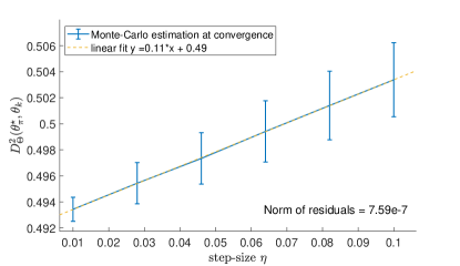
Figure 4: Monte Carlo approximations of the mean distance at convergence in Theorem 13

Similarly to Figure 2, Figure 4 illustrates Theorem 7. To this end, 1000 replications of the experiment derived for Figure 3 are performed, obtaining $\{(\theta_{n}^{(i)})\,:\,i\in\{1,\dots,1000\}\}$ for $n=\lceil 50/\upeta\rceil$ and $\upeta\in\{1,2.8,4.6,6.4,8.2,10\}\times 10^{-2}$. We estimate, with these samples, the mean and the variance of $D_{\Theta}^{2}(\theta,{\theta^{\star}_{\pi}})$, for $\theta$ following the stationary distribution $\mu^{\upeta}$. We observe that the mean and variance are both linear w.r.t. the step-size $\upeta$, indicating that the iterates of the SA scheme remain in a neighborhood of diameter $\mathcal{O}(\upeta^{1/2})$ to the ground truth.

Even though the setting of this experiment goes beyond the assumptions of Theorem 7, it suggests that such a result may be applicable also in the setting of Theorem 13. The proof of such a result is left for future work.

Appendix E Background on Markov chain theory and Riemannian geometry

We give here some useful definitions and results that are used throughout the paper.

E.1 Markov chain notions

We refer to Meyn and Tweedie, (2009) for a general introduction to Markov chains in general state space. Let $(\mathsf{Y},\mathcal{Y})$ be a measurable state space and $P$ be a Markov kernel on $\mathsf{Y}\times\mathcal{Y}$. Consider for any $y\in\mathsf{Y}$, the distribution $\mathbb{P}_{y}$ of the canonical Markov chain $(Y_{n})_{n\in\mathbb{N}}$ corresponding to $P$ and starting from $y$ on the canonical space $(\mathsf{Y}^{\mathbb{N}},\mathcal{Y}^{\otimes\mathbb{N}})$. Denote by $\mathbb{E}_{y}$ the corresponding expectation.

Denote for any $\mathsf{A}\in\mathcal{Y}$, $\tau_{\mathsf{A}}=\inf\{{l}\geq 1\,:\,Y_{l}\in\mathsf{A}\}$ and $N_{\mathsf{A}}=\sum_{{l}=1}^{+\infty}\mathbbm{1}_{\{\mathsf{A}\}}(Y_{l})$.

We say that $(Y_{n})_{n\in\mathbb{N}}$ is $\psi$-irreducible if there exists a measure $\psi$ on $\mathcal{Y}$ such that whenever $\psi(\mathsf{A})>0$, we have $\mathbb{P}_{y}(\tau_{\mathsf{A}}<\infty)>0$ for any $y\in\mathsf{Y}$. Moreover, a set $\mathsf{A}\in\mathcal{Y}$ is called Harris-recurrent if $\mathbb{P}_{y}(N_{\mathsf{A}}=\infty)=1$ for any $y\in\mathsf{A}$. Finally, a chain $(Y_{n})_{n\in\mathbb{N}}$ is called Harris-recurrent if it is $\psi$-irreducible and every set $\mathsf{A}\in\mathcal{Y}$ such that $\psi(\mathsf{A})>0$ is Harris-recurrent.

Let $\overline{V}:\mathsf{Y}\to\left[1,+\infty\right)$. We say that $P$ is $\overline{V}$-uniformly geometrically ergodic if there exist $\rho\in\left[0,1\right)$ and $C\geq 0$ such that for any $y\in\mathsf{Y}$ and $k\in\mathbb{N}$, $\left\|\updelta_{y}P^{k}-\mu\right\|_{\overline{V}}\leq C\rho^{k}\overline{V}(y)$, where $\left\|\cdot\right\|_{\overline{V}}$ is defined for two probability measures $\nu_{1},\nu_{2}$ on $(\mathsf{Y},\mathcal{Y})$ by $\left\|\nu_{1}-\nu_{2}\right\|_{\overline{V}}=\sup\{\left|\nu_{1}(g)-\nu_{2}(g)\right|\,:\,\sup_{\mathsf{Y}}\{\left|g\right|/\overline{V}\}\leq 1\}$.

E.2 Useful results from Riemannian geometry

We now give definitions and auxiliary results related to tensor fields along curves, their derivatives, and Taylor expansions on Riemannian manifolds.

Let $\mathsf{M}$ be a smooth manifold with or without boundary. Given a smooth curve $\upgamma:I\to\mathsf{M}$ defined on an interval $I$, and any $k,l\in\mathbb{N}$, a $(k,l)$-tensor field along $\upgamma$ is a continuous map $F:I\to\mathrm{T}^{(k,l)}\mathrm{T}\mathsf{M}$, such that $F(t)\in\mathrm{T}^{(k,l)}(\mathrm{T}_{\upgamma(t)}\mathsf{M})$ for any $t\in I$, where $\mathrm{T}^{(k,l)}\mathrm{T}\mathsf{M}$ is the bundle of $(k,l)$-tensors on $\mathsf{M}$, see e.g. (Lee,, 2019, Appendix B). A vector field $Y$ along $\upgamma$ is a $(1,0)$-tensor field, in which case for any $t\in I$, $Y(t)$ is just a tangent vector in $\mathrm{T}_{\upgamma(t)}\mathsf{M}$. We say that a tensor field $F$ along $\upgamma$ is extendible if there exists a tensor field $\tilde{F}$ defined on a neighborhood of $\upgamma(I)$ such that $F=\tilde{F}\circ\upgamma$.

We let $\mathfrak{X}^{k,l}(\upgamma)$ denote the set of smooth $(k,l)$-tensor fields along $\upgamma$, and $\mathfrak{X}(\upgamma)=\mathfrak{X}^{1,0}(\upgamma)$ denote the set of smooth vector fields along $\upgamma$. In particular, $\mathfrak{X}^{0,0}(\upgamma)$ is the set of smooth functions $g:I\to\upgamma(I)\times\mathbb{R}$ such that for any $t\in I$, $g(t)=(\upgamma(t),f(t))$ for some smooth function $f:I\to\mathbb{R}$ and therefore can be identified with the set of smooth functions $f:I\to\mathbb{R}$. In the sequel, we adopt if no confusion is possible this identification. We extend to tensor fields along $\upgamma$ the following definition of the trace on tensors. For any $(k,l)$-tensor $T$, we denote by $\operatorname{Tr}_{\square,\triangle}(T)$ the $(k-1,l-1)$-tensor with component of index $(i_{1},\ldots,i_{k-1},j_{1},\ldots,j_{l-1})$, given by $\sum_{m=1}^{d}T_{i_{1},\ldots,i_{\square-1},m,i_{\square},\ldots,i_{k-1}}^{j_{1},\ldots,j_{\triangle-1},m,j_{\triangle},\ldots,j_{l-1}}$. In particular, for any $\omega\in\mathfrak{X}^{0,1}(\upgamma),Y\in\mathfrak{X}(\upgamma)$,

$$\operatorname{Tr}_{(1,1)}(\omega\otimes Y)=\omega(Y)\;.$$ (203)

Also, for any $F\in\mathfrak{X}^{k,l}(\upgamma)$, any $\omega^{1},\ldots,\omega^{k_{0}}\in\mathfrak{X}^{0,1}(\upgamma)$ and $Y_{1},\dots,Y_{l_{0}}\in\mathfrak{X}(\upgamma)$, with $k_{0}\leq k,l_{0}\leq l$, denote by $[F\,:\,\omega^{1}\otimes\cdots\otimes\omega^{k_{0}}\otimes Y_{1}\otimes\cdots\otimes Y_{l_{0}}]$, the $(k-k_{0},l-l_{0})$ smooth tensor field along $\upgamma$ defined by the induction:

$$[F\,:\,\omega^{\otimes 1:i}] =\operatorname{Tr}_{(1,l+1)}([F\,:\,\omega^{\otimes 1:(i-1)}]\otimes\omega^{i})$$ (204)

$$[F\,:\,\omega^{\otimes 1:{k_{0}}}\otimes Y_{\otimes 1:j}] =\operatorname{Tr}_{(k-{k_{0}}+1,1)}([F\,:\,\omega^{\otimes 1:{k_{0}}}\otimes Y_{\otimes 1:(j-1)}]\otimes Y_{j})\;,$$ (205)

setting $\omega^{\otimes 1:i}=\omega^{1}\otimes\cdots\otimes\omega^{i}$, $Y_{\otimes 1:j}=Y_{1}\otimes\cdots\otimes Y_{j}$. Note that for any $\omega^{k-{k_{0}}+1},\ldots,\omega^{k}\in\mathfrak{X}^{0,1}(\upgamma)$ and $Y_{l-{l_{0}}+1},\ldots,Y_{l}\in\mathfrak{X}(\upgamma)$,

$$[F\,:\,\omega^{\otimes 1:{k_{0}}}\otimes Y_{\otimes 1:{l_{0}}}](\omega^{k-{k_{0}}+1},\ldots,\omega^{k},Y_{l-{l_{0}}+1},\ldots,Y_{l})=F(\omega^{1},\ldots,\omega^{k},Y_{1},\ldots,Y_{l})\;.$$ (206)

Proposition 27.

Let $\mathsf{M}$ be a smooth manifold with or without border, $\nabla$ be a connection on $\mathrm{T}\mathsf{M}$ and $\upgamma:I\to\mathsf{M}$ a smooth curve defined on an interval $I$. Then, for any $k,l\in\mathbb{N}$, $\nabla$ determines an operator $\mathrm{D}_{t}:\mathfrak{X}^{k,l}(\upgamma)\to\mathfrak{X}^{k,l}(\upgamma)$, satisfying the following conditions.

1. On $\mathfrak{X}(\upgamma)$, $\mathrm{D}_{t}$ is the usual covariant derivative along $\upgamma$, see (Lee,, 2019, Theorem 4.24).

2. On $\mathfrak{X}^{0,0}(\upgamma)$, $\mathrm{D}_{t}$ is the usual derivative for real functions, i.e. for any $f\in\mathfrak{X}^{0,0}(\upgamma)$, $\mathrm{D}_{t}f=\mathrm{d}f/\mathrm{d}t$.

3. For any $F\in\mathfrak{X}^{k,l}(\upgamma)$, any $\omega^{1},\dots,\omega^{k}\in\mathfrak{X}^{0,1}(\upgamma)$ and any $Y_{1},\dots,Y_{l}\in\mathfrak{X}(\upgamma)$,

   $$(\mathrm{D}_{t}F)\left(\omega^{1},\dots,\omega^{k},Y_{1},\dots,Y_{l}\right) =\frac{\mathrm{d}}{\mathrm{d}t}\left[F\left(\omega^{1},\dots,\omega^{k},Y_{1},\dots,Y_{l}\right)\right]$$ (207)

   $$\quad-\sum_{i=1}^{k}F\left(\omega^{1},\dots,\omega^{i-1},\mathrm{D}_{t}\omega^{i},\omega^{i+1},\dots,\omega^{k},Y_{1},\dots,Y_{l}\right)$$

   $$\quad-\sum_{j=1}^{l}F\left(\omega^{1},\dots,\omega^{k},Y_{1},\dots,Y_{j-1},\mathrm{D}_{t}Y_{j},Y_{j+1},\dots,Y_{l}\right)\;.$$

In particular, $\mathrm{D}_{t}$ satisfies these additional properties.

1. $\mathrm{D}_{t}$ satisfies the product rule, i.e. for any $f\in\mathfrak{X}^{0,0}(\upgamma),F\in\mathfrak{X}^{k,l}(\upgamma),$

   $$\mathrm{D}_{t}\left(fF\right)=\left(\frac{\mathrm{d}}{\mathrm{d}t}f\right)F+f\mathrm{D}_{t}F\;.$$ (208)

2. For any $k_{1},l_{1},k_{2},l_{2}\in\mathbb{N}$, and any $F\in\mathfrak{X}^{k_{1},l_{1}}(\upgamma),G\in\mathfrak{X}^{k_{2},l_{2}}(\upgamma)$,

   $$\mathrm{D}_{t}(F\otimes G)=\mathrm{D}_{t}F\otimes G+F\otimes\mathrm{D}_{t}G\;.$$ (209)

3. For any positive integers $k_{0}\leq k,l_{0}\leq l$, $F\in\mathfrak{X}^{k,l}(\upgamma)$,

   $$\mathrm{D}_{t}\left\{\operatorname{Tr}_{(k_{0},l_{0})}(F)\right\}=\operatorname{Tr}_{(k_{0},l_{0})}\left(\mathrm{D}_{t}F\right)\;.$$ (210)

4. Let $F\in\mathfrak{X}^{k,l}$ be an extendible tensor field, i.e., such that there exists a $(k,l)$-tensor field $\tilde{F}$ defined on a neighborhood of $\upgamma(I)$ satisfying for any $t\in I$, $F(t)=\tilde{F}(\upgamma(t))$. Then, for any $t\in I$,

   $$\mathrm{D}_{t}F(t)=\nabla_{\dot{\upgamma}(t)}\tilde{F}({\upgamma(t)})\;.$$ (211)

Finally, if $\tilde{\mathrm{D}}_{t}:\mathfrak{X}^{k,l}(\upgamma)\to\mathfrak{X}^{k,l}(\upgamma)$ is another operator satisfying (a),(b),(i),(ii) and (iii), then $\mathrm{D}_{t}=\tilde{\mathrm{D}}_{t}$.

Proof.

Let $k,l\in\mathbb{N}$. Note first that (a)-(b) and (207) define $\mathrm{D}_{t}F$ for any $F\in\mathfrak{X}^{k,l}(\upgamma)$, setting for any $\omega\in\mathfrak{X}^{0,1}(\upgamma)$ and $Y\in\mathfrak{X}(\upgamma)$,

$$\left[\mathrm{D}_{t}\omega\right](Y)={\mathrm{d}}\left[\omega(Y)\right]/{\mathrm{d}t}-\omega(\mathrm{D}_{t}Y)\;.$$ (212)

We now show that $\mathrm{D}_{t}F\in\mathfrak{X}^{k,l}$, which will imply that $\mathrm{D}_{t}:\mathfrak{X}^{k,l}\to\mathfrak{X}^{k,l}$. Second, we establish that (i)-(ii)-(iii)-(iv) are satisfied. We conclude the proof by proving uniqueness of $\mathrm{D}_{t}$.

Using (Lee,, 2019, Lemma B.6), to show that $\mathrm{D}_{t}F\in\mathfrak{X}^{k,l}$ it is enough to prove that $\mathrm{D}_{t}F$ is multilinear over $\mathfrak{X}^{0,0}(\upgamma)$. For that, we start proving (i) on $\mathfrak{X}^{0,1}(\upgamma)$. Let $\omega\in\mathfrak{X}^{0,1}(\upgamma),f\in\mathfrak{X}^{0,0}(\upgamma)$ and $Y\in\mathfrak{X}(\upgamma)$, then by (212),

$$\left[\mathrm{D}_{t}(f\omega)\right](Y)={\mathrm{d}}\left[f\omega(Y)\right]/{\mathrm{d}t}-f\omega\left(\mathrm{D}_{t}Y\right)=\left[{\mathrm{d}}f/{\mathrm{d}t}\right]\omega(Y)+f\left[\mathrm{D}_{t}\omega\right](Y)\;,$$ (213)

which proves (i) on $\mathfrak{X}^{0,1}(\upgamma)$. Now, let $k,l\in\mathbb{N},F\in\mathfrak{X}^{k,l}(\upgamma),\omega^{1},\dots,\omega^{k}\in\mathfrak{X}^{0,1}(\upgamma),Y_{1},\dots,Y_{l}\in\mathfrak{X}(\upgamma)$. Let $f\in\mathfrak{X}^{0,0}(\upgamma)$ and $k_{0}\in\mathbb{N}^{*},k_{0}\leq k$. We have, using the multilinearity of $F$ over $\mathfrak{X}^{0,0}(\upgamma)$, the definition of $\mathrm{D}_{t}$ (207), and (213)

$$\left[\mathrm{D}_{t}F\right]\left(\omega^{1},\dots,\omega^{k_{0}-1},f\omega^{k_{0}},\omega^{k_{0}+1},\dots,\omega^{k},Y_{1},\dots,Y_{l}\right)$$ (214)

$$\qquad=\frac{\mathrm{d}}{\mathrm{d}t}\left[F\left(\omega^{1},\dots,\omega^{k_{0}-1},f\omega^{k_{0}},\omega^{k_{0}+1},\dots,\omega^{k},Y_{1},\dots,Y_{l}\right)\right]$$ (215)

$$\qquad\qquad\qquad\quad-\sum_{i=1,i\neq k_{0}}^{k}fF\left(\omega^{1},\dots,\omega^{i-1},\mathrm{D}_{t}\omega^{i},\omega^{i+1},\dots\omega^{k},Y_{1},\dots,Y_{l}\right)$$ (216)

$$\qquad\qquad\qquad\quad-F\left(\omega^{1},\dots,\omega^{k_{0}-1},\mathrm{D}_{t}(f\omega^{k_{0}}),\omega^{k_{0}+1},\dots,\omega^{k},Y_{1},\dots,Y_{l}\right)$$ (217)

$$\qquad\qquad\qquad\quad-\sum_{j=1}^{l}fF\left(\omega^{1},\dots,\omega^{k},Y_{1},\dots,Y_{j-1},\mathrm{D}_{t}Y_{j},Y_{j+1},\dots,Y_{l}\right)$$ (218)

$$\qquad=\left[\frac{\mathrm{d}}{\mathrm{d}t}f\right]\left\{F\left(\omega^{1},\dots,\omega^{k},Y_{1},\dots,Y_{k}\right)-F\left(\omega^{1},\dots,\omega^{k},Y_{1},\dots,Y_{k}\right)\right\}$$ (219)

$$\qquad\qquad\qquad\quad+f\left[\mathrm{D}_{t}F\right]\left(\omega^{1},\dots,\omega^{k},Y_{1},\dots,Y_{l}\right)$$ (220)

$$\qquad=f\left[\mathrm{D}_{t}F\right]\left(\omega^{1},\dots,\omega^{k},Y_{1},\dots,Y_{l}\right)\;.$$ (221)

The same arguments apply if we replace $Y_{l_{0}}$ with $fY_{l_{0}}$, for some $l_{0}\leq l$. Thus, using (Lee,, 2019, Lemma B.6), $\mathrm{D}_{t}F\in\mathfrak{X}^{k,l}$.

Next, regarding (i), using the definition of $\mathrm{D}_{t}$,

$$\left[\mathrm{D}_{t}fF\right]\left(\omega^{1},\dots,\omega^{k},Y_{1},\dots,Y_{l}\right) =\left[\frac{\mathrm{d}}{\mathrm{d}t}f\right]F\left(\omega^{1},\dots,\omega^{k},Y_{1},\dots,Y_{l}\right)$$ (222)

$$\quad+f\left[\mathrm{D}_{t}F\right]\left(\omega^{1},\dots,\omega^{k},Y_{1},\dots,Y_{l}\right)\;,$$ (223)

thus proving (i). Moreover, we prove (ii). Let $k_{1},l_{1},k_{2},l_{2}\in\mathbb{N}$ and $F\in\mathfrak{X}^{k_{1},l_{1}}(\upgamma),G\in\mathfrak{X}^{k_{2},l_{2}}(\upgamma)$, $\omega^{1},\dots,\omega^{k_{1}+k_{2}}\in\mathfrak{X}^{0,1}(\upgamma),Y_{1},\dots,Y_{l_{1}+l_{2}}\in\mathfrak{X}(\upgamma)$. Setting

$$f=F(\omega^{1},\dots,\omega^{k_{1}},Y_{1},\dots,Y_{l_{1}})\text{ and }g=G(\omega^{k_{1}+1},\dots,\omega^{k_{1}+k_{2}},Y_{l_{1}+1},\dots,Y_{l_{1}+l_{2}})\;,$$

we have

$$\left[\mathrm{D}_{t}(F\otimes G)\right]\left(\omega^{1},\dots,\omega^{k_{1}+k_{2}},Y_{1},\dots,Y_{l_{1}+l_{2}}\right)$$ (224)

$$\quad=\frac{\mathrm{d}}{\mathrm{d}t}\left[fg\right]-\left[\sum_{i=1}^{k_{1}}F\left(\omega^{1},\dots,\omega^{i-1},\mathrm{D}_{t}\omega^{i},\omega^{i+1},\dots,\omega^{k_{1}},Y_{1},\dots,Y_{l_{1}}\right)\right.$$ (225)

$$\quad\quad+\left.\sum_{j=1}^{l_{1}}F\left(\omega^{1},\dots,\omega^{k_{1}},Y_{1},\dots,Y_{j-1},\mathrm{D}_{t}Y_{j},Y_{j+1},\dots,Y_{l_{1}}\right)\right]g$$ (226)

$$\qquad-f\left[\sum_{i=1}^{k_{2}}G\left(\omega^{k_{1}+1},\dots,\omega^{k_{1}+i-1},\mathrm{D}_{t}\omega^{k_{1}+i},\omega^{k_{1}+i+1},\dots,\omega^{k_{1}+k_{2}},Y_{l_{1}+1},\dots,Y_{l_{1}+l_{2}}\right)\right.$$ (227)

$$\qquad+\left.\sum_{j=1}^{l_{2}}G\left(\omega^{k_{1}+1},\dots,\omega^{k_{1}+k_{2}},Y_{l_{1}+1},\dots,Y_{l_{1}+j-1},\mathrm{D}_{t}Y_{l_{1}+j},Y_{l_{1}+j+1},\dots,Y_{l_{1}+l_{2}}\right)\right]$$ (228)

$$\quad=\left[\mathrm{D}_{t}F\right]\left(\omega^{1},\dots,\omega^{k_{1}},Y_{1},\dots,Y_{l_{1}}\right)g+f\left[\mathrm{D}_{t}G\right]\left(\omega^{k_{1}+1},\dots,\omega^{k_{1}+k_{2}},Y_{l_{1}+1},\dots,Y_{l_{1}+l_{2}}\right)$$ (229)

$$\quad=\left[\mathrm{D}_{t}F\otimes G+F\otimes\mathrm{D}_{t}G\right]\left(\omega^{1},\dots,\omega^{k_{1}+k_{2}},Y_{1},\dots,Y_{l_{1}+l_{2}}\right)\;,$$ (230)

which proves (ii). Furthermore, to prove (iii), let $t_{0}\in I$ and $(\mathbf{b}_{i})_{i\in\{1,\dots,d\}}$ be a basis of $\mathrm{T}_{\upgamma(t_{0})}\Theta$. Using (a) and (Lee,, 2019, Theorem 4.32), define for any $i\in\{1,\dots,d\}$ and $t\in I$,

$$e_{i}(t)=\mathrm{T}_{t_{0},t}^{\upgamma}\mathbf{b}_{i}\;,$$ (231)

where $\mathrm{T}_{t_{0},t}^{\upgamma}$ denotes the parallel transport map along $\upgamma$ from $\mathrm{T}_{\upgamma(t_{0})}\Theta$ to $\mathrm{T}_{\upgamma(t)}\Theta$. As the parallel transport map is an isomorphism, $(e_{i}(t))_{i\in\{1,\dots,d\}}$ is a basis of $\mathrm{T}_{\upgamma(t)}\Theta$, for any $t\in I$. Therefore the family of smooth vector fields $(e_{i})_{i\in\{1,\dots,d\}}$ is a parallel frame along $\upgamma$ (with respect to $\nabla$). Denote $(\varepsilon^{j})_{j\in\{1,\dots,d\}}$ its dual coframe. Using (212) on $Y=e_{i},\omega=\varepsilon^{j}$, for any $i,j\in\{1,\dots,d\}$, shows that the coframe $(\varepsilon^{j})_{j\in\{1,\dots,d\}}$ is parallel along $\upgamma$. Note that for $(e_{i})_{i\in\{1,\dots,d\}}$ and $(\varepsilon^{j})_{j\in\{1,\dots,d\}}$ to be well defined, we have used $\nabla$, as well as the operator $\mathrm{D}_{t}$ on $\mathfrak{X}(\upgamma)$ and $\mathfrak{X}^{0,1}(\upgamma)$.

Let $k,l\in\mathbb{N}^{*}$ such that $k_{0}\leq k,l_{0}\leq l$, and let $F\in\mathfrak{X}^{k,l}(\upgamma)$. There exist a family of functions $\{F^{j_{1},\dots,j_{l}}_{i_{1},\dots,i_{k}}\in\mathfrak{X}^{0,0}(\upgamma)\,:\,i_{1},\dots,i_{k},j_{1},\dots,j_{l}\in\{1,\dots,d\}\}$ such that

$$F=\sum_{i_{1},\dots,i_{k}=1}^{d}\sum_{j_{1},\dots,j_{l}=1}^{d}F^{j_{1},\dots,j_{l}}_{i_{1},\dots,i_{k}}\bigotimes_{\triangle=1}^{k}e_{i_{\triangle}}\bigotimes_{\square=1}^{l}\varepsilon^{j_{\square}}\;.$$ (232)

Since the frame and its dual coframe are parallel along $\upgamma$, for any $i\in\{1,\dots,d\}$ $\mathrm{D}_{t}e_{i}=0$ and $\mathrm{D}_{t}\varepsilon^{i}=0$. Combining this fact with (i) and (ii) gives

$$\mathrm{D}_{t}F=\sum_{i_{1},\dots,i_{k}=1}^{d}\sum_{j_{1},\dots,j_{l}=1}^{d}\left[\frac{\mathrm{d}}{\mathrm{d}t}F^{j_{1},\dots,j_{l}}_{i_{1},\dots,i_{k}}\right]\bigotimes_{\triangle=1}^{k}e_{i_{\triangle}}\bigotimes_{\square=1}^{l}\varepsilon^{j_{\square}}\;.$$ (233)

Let $k_{0},l_{0}\in\mathbb{N}^{*}$ such that $k_{0}\leq k,l_{0}\leq l$, then by definition of $\operatorname{Tr}_{(k_{0},l_{0})}$, for any $i_{1},\dots,i_{k-1},j_{1},\dots,j_{l-1}\in\{1,\dots,d\}$,

$$\operatorname{Tr}_{(k_{0},l_{0})}(F)^{j_{1},\dots,j_{l-1}}_{i_{1},\dots,i_{k-1}}=\sum_{m=1}^{d}F^{j_{1},\dots,j_{l_{0}-1},m,j_{l_{0}},\dots,j_{l-1}}_{i_{1},\dots,i_{k_{0}-1},m,i_{k_{0}},\dots,i_{k-1}}\;.$$ (234)

We remind the reader that $\operatorname{Tr}_{(k_{0},l_{0})}(F)$ does not depend on the choice of coordinates (Lee,, 2019, Appendix B). Thus, using (233) and (234), we have

$$\mathrm{D}_{t}\left[\operatorname{Tr}_{(k_{0},l_{0})}(F)\right] =\sum_{i_{1},\dots,i_{k-1}=1}^{d}\sum_{j_{1},\dots,j_{l-1}=1}^{d}\frac{\mathrm{d}}{\mathrm{d}t}\left[\operatorname{Tr}_{(k_{0},l_{0})}(F)^{j_{1},\dots,j_{l-1}}_{i_{1},\dots,i_{k-1}}\right]\bigotimes_{\triangle=1}^{k-1}e_{i_{\triangle}}\bigotimes_{\square=1}^{l-1}\varepsilon^{j_{\square}}$$ (235)

$$=\sum_{i_{1},\dots,i_{k-1}=1}^{d}\sum_{j_{1},\dots,j_{l-1}=1}^{d}\sum_{m=1}^{d}\frac{\mathrm{d}}{\mathrm{d}t}F^{j_{1},\dots,j_{l_{0}-1},m,j_{l_{0}},\dots,j_{l-1}}_{i_{1},\dots,i_{k_{0}-1},m,i_{k_{0}},\dots,i_{k-1}}\bigotimes_{\triangle=1}^{k-1}e_{i_{\triangle}}\bigotimes_{\square=1}^{l-1}\varepsilon^{j_{\square}}$$ (236)

$$=\operatorname{Tr}_{(k_{0},l_{0})}\left(\mathrm{D}_{t}F\right)\;,$$ (237)

thus proving (iii).

To prove (iv), first for any $f\in\mathfrak{X}^{(0,0)}(\upgamma)$, extendible in $\tilde{f}$, we have by composition and definition of the covariant derivative, that for any $t\in[0,1]$,

$$(\mathrm{d}f/\mathrm{d}t)(t)=\mathrm{d}\tilde{f}_{\upgamma(t)}(\dot{\upgamma}(t))=\nabla_{\dot{\upgamma}(t)}\tilde{f}(\upgamma(t))\;.$$ (238)

Also, using (Lee,, 2019, Theorem 4.24-(iii)) gives (iv) for any $Y\in\mathfrak{X}(\upgamma)$. Combining (238), (212), its counterpart for tensor fields defined over a manifold (Lee,, 2019, Proposition 4.15-(a)) and (iv) over $\mathfrak{X}(\upgamma)$, proves (iv) over $\mathfrak{X}^{(0,1)}(\upgamma)$. Now, for any $k,l\in\mathbb{N}$, using (iv) over $\mathfrak{X}(\upgamma)$ and $\mathfrak{X}^{(0,1)}(\upgamma)$ combined with (207) and its counterpart for tensor fields defined over a manifold (Lee,, 2019, Equation (4.12)) gives (iv) over $\mathfrak{X}^{(k,l)}(\upgamma)$.

Finally, we address uniqueness. Suppose now that $\tilde{\mathrm{D}}_{t}$ is an operator on $\mathfrak{X}^{k,l}(\upgamma)$ that satisfies (a),(b),(i),(ii) and (iii). First, (a) and (b) show that $\mathrm{D}_{t}$ and $\tilde{\mathrm{D}}_{t}$ coincide on $\mathfrak{X}^{0,0}(\upgamma)$ and $\mathfrak{X}(\upgamma)$. Second, for any $Y\in\mathfrak{X}(\upgamma),\omega\in\mathfrak{X}^{0,1}(\upgamma)$, writing $\omega(Y)=\operatorname{Tr}_{(1,1)}(Y\otimes\omega)$ and using (iii) gives

$$\tilde{\mathrm{D}}_{t}\omega=\mathrm{d}[\omega(Y)]/\mathrm{d}t-\omega(\tilde{\mathrm{D}}_{t}Y)=\mathrm{D}_{t}\omega\;,$$ (239)

using (212). Thus, $\tilde{\mathrm{D}}_{t}$ and $\mathrm{D}_{t}$ also agree on $\mathfrak{X}^{0,1}(\upgamma)$. Therefore, the frame $(e_{i})_{i\in\{1,\dots,d\}}$ and its dual coframe $(\varepsilon^{j})_{j\in\{1,\dots,d\}}$ are also parallel with respect to $\tilde{\mathrm{D}}_{t}$ along $\upgamma$. Let $F\in\mathfrak{X}^{k,l}(\upgamma)$, then using (i) and (ii) shows that (233) holds for the operator $\tilde{\mathrm{D}}_{t}$, proving that $\mathrm{D}_{t}F=\tilde{\mathrm{D}}_{t}F$. This concludes the proof.

∎

Lemma 28.

Let $\mathsf{M}$ be a smooth manifold and $\nabla$ be a connection on $\mathrm{T}\mathsf{M}$. Let $\upgamma:[0,1]\to\mathsf{M}$ be a smooth curve and denote $\mathrm{D}_{t}$ the covariant derivative operator along $\upgamma$ associated with $\nabla$, defined in Proposition 27. Let $F\in\mathfrak{X}^{k,l}(\upgamma)$, $\omega^{1},\ldots,\omega^{k_{0}}\in\mathfrak{X}^{0,1}(\upgamma)$ and $Y_{1},\dots,Y_{l_{0}}\in\mathfrak{X}(\upgamma)$, with ${k_{0}}\leq k,{l_{0}}\leq l$. Then, we have

$$\mathrm{D}_{t}\left([F:\omega^{\otimes 1:{k_{0}}}\otimes Y_{\otimes 1:{l_{0}}}]\right) =[\mathrm{D}_{t}F:\omega^{\otimes 1:{k_{0}}}\otimes Y_{\otimes 1:{l_{0}}}]$$ (240)

$$\qquad+\sum_{i=1}^{k_{0}}[F:\omega^{\otimes 1:(i-1)}\otimes\mathrm{D}_{t}\omega^{i}\otimes\omega^{(i+1):{k_{0}}}\otimes Y_{\otimes 1:{l_{0}}}]$$

$$\qquad+\sum_{j=1}^{l_{0}}[F:\omega^{\otimes 1:{k_{0}}}\otimes Y_{\otimes 1:(j-1)}\otimes\mathrm{D}_{t}Y_{j}\otimes Y_{\otimes(j+1):{l_{0}}}]\;.$$

Proof.

Let $F$ be a smooth $(k,l)$-tensor field along $\upgamma$. We show (240) by induction. Following the recursive definition of the contraction in (204), we prove it by induction on ${k_{0}}\in\mathbb{N}^{*},{k_{0}}\leq k$, for any $\omega^{1},\dots,\omega^{k_{0}}\in\mathfrak{X}^{0,1}(\upgamma)$.

The case ${k_{0}}=1$ follows from Proposition 27-(ii) and (iii), combined with the definition in (204),

$$\mathrm{D}_{t}\left[F:\omega^{1}\right] =\mathrm{D}_{t}\operatorname{Tr}_{(1,l+1)}(F\otimes\omega^{1})$$ (241)

$$=\operatorname{Tr}_{(1,l+1)}(\mathrm{D}_{t}[F\otimes\omega^{1}])$$ (242)

$$=\operatorname{Tr}_{(1,l+1)}(\mathrm{D}_{t}F\otimes\omega^{1}+F\otimes\mathrm{D}_{t}\omega^{1})$$ (243)

$$=\left[\mathrm{D}_{t}F:\omega^{1}\right]+\left[F:\mathrm{D}_{t}\omega^{1}\right]\;,$$ (244)

where we have used the linearity of $\operatorname{Tr}$. Now assume there exists ${k_{0}}\in\{1,\dots,k-1\}$ such that (240) holds for any smooth $1$ forms $\omega^{1},\dots,\omega^{k_{0}}$ and ${l_{0}}=0$. Moreover, consider any smooth $1$ forms $\omega^{1},\dots,\omega^{{k_{0}}+1}$. Then, using the same arguments as for the case ${k_{0}}=1$ and the induction hypothesis, we obtain

$$\mathrm{D}_{t}\left[F:\omega^{\otimes 1:({k_{0}}+1)}\right] =\mathrm{D}_{t}\operatorname{Tr}_{(1,l+1)}\left(\left[F:\omega^{\otimes 1:{k_{0}}}\right]\otimes\omega^{{k_{0}}+1}\right)$$ (245)

$$=\operatorname{Tr}_{(1,l+1)}\left(\mathrm{D}_{t}\left[F:\omega^{\otimes 1:{k_{0}}}\right]\otimes\omega^{{k_{0}}+1}\right)+\operatorname{Tr}_{(1,l+1)}\left(\left[F:\omega^{\otimes 1:{k_{0}}}\right]\otimes\mathrm{D}_{t}\omega^{{k_{0}}+1}\right)$$ (246)

$$=\operatorname{Tr}_{(1,l+1)}\left(\left[\mathrm{D}_{t}F:\omega^{\otimes 1:{k_{0}}}\right]\otimes\omega^{{k_{0}}+1}\right)+\left[F:\omega^{\otimes 1:{k_{0}}}\otimes\mathrm{D}_{t}\omega^{{k_{0}}+1}\right]$$ (247)

$$\quad+\sum_{i=1}^{{k_{0}}}\operatorname{Tr}_{(1,l+1)}\left(\left[F:\omega^{\otimes 1:(i-1)}\otimes\mathrm{D}_{t}\omega^{i}\otimes\omega^{\otimes(i+1):{k_{0}}}\right]\otimes\omega^{{k_{0}}+1}\right)$$ (248)

$$=\left[\mathrm{D}_{t}F:\omega^{\otimes 1:({k_{0}}+1)}\right]+\sum_{i=1}^{{k_{0}}+1}\left[F:\omega^{\otimes 1:(i-1)}\otimes\mathrm{D}_{t}\omega^{i}\otimes\omega^{\otimes(i+1):({k_{0}}+1)}\right]\;.$$ (249)

Subsequently, using the recursive definition of the contraction in (205), we prove (240) by induction on ${l_{0}}\in\mathbb{N}^{*},{l_{0}}\leq l$ for any ${k_{0}}\leq k$ and any $\omega^{1},\dots,\omega^{k_{0}}\in\mathfrak{X}^{0,1}(\upgamma)$. Let $Y_{1}\in\mathfrak{X}(\upgamma)$. Then, using once again Proposition 27-(ii) and (iii), (205), and (240) in the case ${l_{0}}=0$ justified above, the case ${l_{0}}=1$ is proven as follows,

$$\mathrm{D}_{t}\left[F:\omega^{\otimes 1:{k_{0}}}\otimes Y_{1}\right] =\operatorname{Tr}_{(k-{k_{0}}+1,1)}\left(\mathrm{D}_{t}\left\{\left[F:\omega^{\otimes 1:{k_{0}}}\right]\otimes Y_{1}\right\}\right)$$ (250)

$$=\operatorname{Tr}_{(k-{k_{0}}+1,1)}\left(\left[\mathrm{D}_{t}F:\omega^{\otimes 1:{k_{0}}}\right]\otimes Y_{1}\right)+\left[F:\omega^{\otimes 1:{k_{0}}}\otimes\mathrm{D}_{t}Y_{1}\right]$$ (251)

$$\quad+\sum_{i=1}^{k_{0}}\operatorname{Tr}_{(k-{k_{0}}+1,1)}\left(\left[F:\omega^{\otimes 1:(i-1)}\otimes\mathrm{D}_{t}\omega^{i}\otimes\omega^{\otimes(i+1):{k_{0}}}\right]\otimes Y_{1}\right)$$ (252)

$$=\left[\mathrm{D}_{t}F:\omega^{\otimes 1:{k_{0}}}\otimes Y_{1}\right]+\sum_{i=1}^{{k_{0}}}\left[F:\omega^{\otimes 1:(i-1)}\otimes\mathrm{D}_{t}\omega^{i}\otimes\omega^{\otimes(i+1):{k_{0}}}\otimes Y_{1}\right]$$ (253)

$$\quad+\left[F:\omega^{\otimes 1:{k_{0}}}\otimes\mathrm{D}_{t}Y_{1}\right]\;.$$ (254)

Furthermore, assume there exists ${l_{0}}\in\{1,\dots,l-1\}$ such that (240) holds for any ${k_{0}}\leq k$, any $\omega^{1},\dots,\omega^{k_{0}}\in\mathfrak{X}^{0,1}(\upgamma)$ and any $Y_{1},\dots,Y_{l_{0}}\in\mathfrak{X}(\upgamma)$. Let $Y_{1},\dots,Y_{{l_{0}}+1}\in\mathfrak{X}(\upgamma)$. Then using the same arguments as for the case ${l_{0}}=1$ and the induction hypothesis, we obtain

$$\mathrm{D}_{t}\left[F:\omega^{\otimes 1:{k_{0}}}\otimes Y_{\otimes 1:({l_{0}}+1)}\right]$$ (255)

$$\qquad=\operatorname{Tr}_{(k-{k_{0}}+1,1)}\left(\mathrm{D}_{t}\left\{\left[F:\omega^{\otimes 1:{k_{0}}}\otimes Y_{\otimes 1:{l_{0}}}\right]\otimes Y_{{l_{0}}+1}\right\}\right)$$ (256)

$$\qquad=\operatorname{Tr}_{(k-{k_{0}}+1,1)}\left(\left[\mathrm{D}_{t}F:\omega^{\otimes 1:{k_{0}}}\otimes Y_{\otimes 1:{l_{0}}}\right]\otimes Y_{{l_{0}}+1}\right)$$ (257)

$$\qquad\quad+\sum_{i=1}^{k_{0}}\operatorname{Tr}_{(k-{k_{0}}+1,1)}\left(\left[F:\omega^{\otimes 1:(i-1)}\otimes\mathrm{D}_{t}\omega^{i}\otimes\omega^{\otimes(i+1):{k_{0}}}\otimes Y_{\otimes 1:{l_{0}}}\right]\otimes Y_{{l_{0}}+1}\right)$$ (258)

$$\qquad\quad+\sum_{j=1}^{l_{0}}\operatorname{Tr}_{(k-{k_{0}}+1,1)}\left(\left[F:\omega^{\otimes 1:{k_{0}}}\otimes Y_{\otimes 1:(j-1)}\otimes\mathrm{D}_{t}Y_{j}\otimes Y_{\otimes(j+1):{l_{0}}}\right]\otimes Y_{{l_{0}}+1}\right)$$ (259)

$$\qquad\quad+\operatorname{Tr}_{(k-{k_{0}}+1,1)}\left(\left[F:\omega^{\otimes 1:{k_{0}}}\otimes Y_{\otimes 1:{l_{0}}}\right]\otimes\mathrm{D}_{t}Y_{{l_{0}}+1}\right)$$ (260)

$$\qquad=\left[\mathrm{D}_{t}F:\omega^{\otimes 1:{k_{0}}}\otimes Y_{\otimes 1:({l_{0}}+1)}\right]+\sum_{i=1}^{k_{0}}\left[F:\omega^{\otimes 1:(i-1)}\otimes\mathrm{D}_{t}\omega^{i}\otimes\omega^{\otimes(i+1):{k_{0}}}\otimes Y_{\otimes 1:({l_{0}}+1)}\right]$$ (261)

$$\qquad\quad+\sum_{j=1}^{{l_{0}}+1}\left[F:\omega^{\otimes 1:{k_{0}}}\otimes Y_{\otimes 1:(j-1)}\otimes\mathrm{D}_{t}Y_{j}\otimes Y_{\otimes(j+1):({l_{0}}+1)}\right]\;,$$ (262)

which concludes the proof. ∎

Theorem 29.

Let $\mathsf{M}$ be a smooth manifold and $\nabla$ be a connection on $\mathrm{T}\mathsf{M}$. Let $\upgamma:[0,1]\to\mathsf{M}$ be a geodesic and $Y:\mathsf{M}\to\mathrm{T}\mathsf{M}$ a smooth vector field. Then, for any $t\in[0,1],n\in\mathbb{N}$,

$$\mathrm{T}_{t0}^{\upgamma}Y(\upgamma(t)) =\sum_{{k_{0}}=0}^{n}(t^{k_{0}}/{k_{0}}!)\left.\nabla^{k_{0}}Y_{\upgamma(0)}\left(\dot{\upgamma}(0),\dots,\dot{\upgamma}(0)\right)\right.$$ (263)

$$\quad+\int_{0}^{t}\left.[(t-s)^{n}/n!]\mathrm{T}_{s0}^{\upgamma}\nabla^{n+1}Y_{\upgamma(s)}\left(\dot{\upgamma}(s),\dots,\dot{\upgamma}(s)\right)\right.\mathrm{d}s\;,$$

where $\mathrm{T}_{t0}^{\upgamma}:\mathrm{T}_{\upgamma(t)}\mathsf{M}\to\mathrm{T}_{\upgamma(0)}\mathsf{M}$ is the parallel transport map along $\upgamma$, and the $(1,{k_{0}})$-tensor field $\nabla^{k_{0}}Y$ is the total derivative of order ${k_{0}}$ of the $(1,0)$-tensor field $Y$.

For a definition of the total covariant derivative, see (Lee,, 2019, Proposition 4.15). Also, in (263), remark that even though $\dot{\upgamma}$ is only a vector field along $\upgamma$, and not a vector field, the value of a vector field $\nabla_{X}Y$ evaluated at $\theta\in\mathsf{M}$ only depends on $X(\theta)$ and on values of $Y$ along smooth curves $\mathrm{c}:[0,1]\to\mathsf{M}$ satisfying $\mathrm{c}(0)=\theta$ and $\dot{\mathrm{c}}(0)=X(\theta)$; by (Lee,, 2019, Proposition 4.26). Therefore the expression $\nabla^{k_{0}}Y_{\upgamma(t)}(\dot{\upgamma}(t),\dots,\dot{\upgamma}(t))$ in Theorem 29 is well defined for any ${k_{0}}\in\mathbb{N},t\in[0,1]$.

Proof.

Consider $\mathpzc{V}:[0,1]\to\mathsf{M}$ the smooth vector field along $\upgamma$ and the function $\varphi:[0,1]\to\mathrm{T}_{\upgamma(0)}\mathsf{M}$ defined by

$$\mathpzc{V}=Y\circ\upgamma\text{ and }\;\varphi:t\mapsto\mathrm{T}_{t0}^{\upgamma}\mathpzc{V}(t)\;.$$ (264)

Then we check by induction on $n\in\mathbb{N}^{*}$ that $\varphi$ is $n$-times differentiable with derivative of order $n$ given for any $t\in[0,1]$ by $\varphi^{(n)}(t)=\mathrm{T}_{t0}^{\upgamma}[\mathrm{D}_{t}^{n}\mathpzc{V}(t)]$ and $\mathrm{D}_{t}^{n}\mathpzc{V}(t)=\nabla^{n}Y_{\upgamma(t)}(\dot{\upgamma}(t),\dots,\dot{\upgamma}(t))$, where $\mathrm{D}_{t}$ is the covariant derivative operator along $\upgamma$ with respect to the connection $\nabla$, defined in Proposition 27.

First, the case $n=1$ is a direct application of (Lee,, 2019, Theorem 4.34, Theorem 4.24) since $Y$ is an extension of $\mathpzc{V}$. Assume now that the property holds for $n\in\mathbb{N}^{*}$. Then, for any $t_{0},t\in[0,1],t\neq t_{0}$, we have

$$\left.\left[\varphi^{(n)}(t)-\varphi^{(n)}(t_{0})\right]\middle/\left(t-t_{0}\right)\right.=\mathrm{T}_{t_{0}0}^{\upgamma}\left.\left[\mathrm{T}_{tt_{0}}^{\upgamma}\mathrm{D}^{n}_{t}\mathpzc{V}(t)-\mathrm{D}^{n}_{t}\mathpzc{V}(t_{0})\right]\middle/\left(t-t_{0}\right)\right.\;.$$ (265)

Now (Lee,, 2019, Theorem 4.34) ensures that the limit of the quantity above exists when $t\to t_{0}$ and in addition this limit is

$$\varphi^{(n+1)}(t_{0})=\mathrm{T}_{t_{0}0}^{\upgamma}\mathrm{D}^{n+1}_{t}\mathpzc{V}(t_{0})\;,$$ (266)

which shows that $\varphi$ is $n+1$ times differentiable on $\left[0,1\right]$. We now show that for any $t\in\left[0,1\right]$, $\mathrm{D}_{t}^{n+1}\mathpzc{V}(t)=\nabla^{n+1}Y_{\upgamma(t)}(\dot{\upgamma}(t),\dots,\dot{\upgamma}(t))$. Using Lemma 28 on the smooth $(1,n)$-tensor field along $\upgamma$ $F=(\nabla^{n}Y)\circ\upgamma$, taking ${k_{0}}=0$ and $n$ times the vector field $\dot{\upgamma}$, we have

$$\mathrm{D}_{t}\left[F:\dot{\upgamma}\otimes\cdots\otimes\dot{\upgamma}\right]=\left[\mathrm{D}_{t}F:\dot{\upgamma}\otimes\cdots\otimes\dot{\upgamma}\right]\;,$$ (267)

since $\mathrm{D}_{t}\dot{\upgamma}=0$ because $\upgamma$ is a geodesic. Also, by (206), $[\mathrm{D}_{t}F:\dot{\upgamma}\otimes\cdots\otimes\dot{\upgamma}]=\mathrm{D}_{t}F(\dot{\upgamma},\dots,\dot{\upgamma})$. Finally, as $\nabla^{n}Y$ is an extension of $F$, using the induction hypothesis and the definition of the total derivative give for any $t\in[0,1]$,

$$\mathrm{D}^{n+1}_{t}\mathpzc{V}(t)=\mathrm{D}_{t}F\left(\dot{\upgamma},\dots,\dot{\upgamma}\right)(t)=\nabla_{\dot{\upgamma}(t)}(\nabla^{n}Y)_{\upgamma(t)}\left(\dot{\upgamma}(t),\dots,\dot{\upgamma}(t)\right)\\ =(\nabla^{n+1}Y)_{\upgamma(t)}\left(\dot{\upgamma}(t),\dots,\dot{\upgamma}(t)\right)\;,$$ (268)

concluding the induction.

Finally, (263) is simply a consequence of Taylor’s formula with integral remainder of the vectorial valued function $\varphi$ identifying $\mathrm{T}_{\upgamma(0)}\mathsf{M}$ with $\mathbb{R}^{d}$. ∎

Proposition 30.

Let $\mathsf{M}$ be a smooth manifold, $\nabla$ be a symmetric connection defined over the smooth vector fields of $\mathsf{M}$. For any smooth function $f:\mathsf{M}\to\mathbb{R}$ and any local coordinates $(u_{i})_{i\in\{1,\dots,d\}}$, we have

$$\nabla\mathrm{Hess}\,f=\sum_{i,j,k=1}^{d}\left\{\partial^{3}_{kij}f-\sum_{l=1}^{d}\left[\Gamma_{ij}^{l}\partial^{2}_{kl}f+\Gamma_{ki}^{l}\partial^{2}_{jl}f+\Gamma_{kj}^{l}\partial^{2}_{il}f\right]-\sum_{m=1}^{d}\partial_{k}\Gamma_{ij}^{m}\partial_{m}f\right.\\ \left.+\sum_{l,m=1}^{d}\left[\Gamma_{kj}^{l}\Gamma_{il}^{m}+\Gamma_{ki}^{l}\Gamma_{lj}^{m}\right]\partial_{m}f\right\}\mathrm{d}u^{i}\otimes\mathrm{d}u^{j}\otimes\mathrm{d}u^{k}\;,$$ (269)

where $(\Gamma_{ij}^{k})_{i,j,k\in\{1,\dots,d\}}$ are the Christoffel symbols in these local coordinates, the local frame and its dual coframe are denoted by $(\partial u_{i})_{i\in\{1,\dots,d\}}$ and $(\mathrm{d}u^{j})_{j\in\{1,\dots,d\}}$.

Proof.

Let $(u_{i})_{i\in\{1,\ldots,d\}}$ be local coordinates. By (Lee,, 2019, Example 4.22), in this chart, we have

$$\mathrm{Hess}\,f=\sum_{i,j=1}^{d}F_{ij}\mathrm{d}u^{i}\otimes\mathrm{d}u^{j}\;,\text{where for any }i,j\in\{1,\dots,d\}\;,\;F_{ij}=\partial_{ij}^{2}f-\sum_{m=1}^{d}\Gamma_{ij}^{m}\partial_{m}f\;.$$ (270)

Applying (Lee,, 2019, Proposition 4.18) on $\mathrm{Hess}\,f$, we obtain that $\nabla\mathrm{Hess}\,f=\sum_{i,j,k=1}^{d}G_{ijk}\mathrm{d}u^{i}\otimes\mathrm{d}u^{j}\otimes\mathrm{d}u^{k}$, where for any $i,j,k\in\{1,\ldots,d\}$,

$$G_{ijk}=\partial_{k}F_{ij}-\sum_{l=1}^{d}\left(\Gamma_{kj}^{l}F_{il}+\Gamma_{ki}^{l}F_{lj}\right)\;.$$ (271)

Expanding the expression above using (270) gives for any $i,j,k\in\{1,\dots,d\}$,

$$G_{ijk}=\partial^{3}_{ijk}f-\sum_{m=1}^{d}\left(\partial_{k}\Gamma_{ij}^{m}\partial_{m}f+\Gamma_{ij}^{m}\partial^{2}_{km}f\right)-\sum_{l=1}^{d}\Gamma_{kj}^{l}\left(\partial^{2}_{il}f-\sum_{m=1}^{d}\Gamma_{il}^{m}\partial_{m}f\right)\\ -\sum_{l=1}^{d}\Gamma_{ki}^{l}\left(\partial^{2}_{lj}f-\sum_{m=1}^{d}\Gamma_{lj}^{m}\partial_{m}f\right)\;.$$ (272)

The desired result is obtained by reordering this equation, which concludes the proof. ∎

References

- Alimisis et al., (2020) Alimisis, F., Orvieto, A., Becigneul, G., and Lucchi, A. (2020). A Continuous-time Perspective for Modeling Acceleration in Riemannian Optimization. volume 108 of Proceedings of Machine Learning Research, pages 1297–1307, Online. PMLR.
- Arnaudon et al., (2012) Arnaudon, M., Dombry, C., Phan, A., and Yang, L. (2012). Stochastic algorithms for computing means of probability measures. Stochastic Processes and their Applications, 122(4):1437 – 1455.
- Bach, (2020) Bach, F. (2020). On the effectiveness of richardson extrapolation in machine learning.
- Bach and Moulines, (2011) Bach, F. and Moulines, E. (2011). Non-asymptotic analysis of stochastic approximation algorithms for machine learning. In Advances in Neural Information Processing Systems 24: 25th Annual Conference on Neural Information Processing Systems 2011. Proceedings of a meeting held 12-14 December 2011, Granada, Spain, pages 451–459.
- Baxter and Bartlett, (2001) Baxter, J. and Bartlett, P. L. (2001). Infinite-horizon policy-gradient estimation. J. Artif. Int. Res., 15(1):319–350.
- Benveniste et al., (1990) Benveniste, A., Métivier, M., and Priouret, P. (1990). Adaptive algorithms and stochastic approximations, volume 22 of Applications of Mathematics (New York). Springer-Verlag, Berlin. Translated from the French by Stephen S. Wilson.
- Bini and Iannazzo, (2013) Bini, D. A. and Iannazzo, B. (2013). Computing the Karcher mean of symmetric positive definite matrices. Linear Algebra and its Applications, 438(4):1700 – 1710. 16th ILAS Conference Proceedings, Pisa 2010.
- Bonnabel, (2013) Bonnabel, S. (2013). Stochastic gradient descent on riemannian manifolds. IEEE Transactions on Automatic Control, 58(9):2217–2229.
- Bottou, (2010) Bottou, L. (2010). Large-scale machine learning with stochastic gradient descent. In Lechevallier, Y. and Saporta, G., editors, Proceedings of the 19th International Conference on Computational Statistics (COMPSTAT’2010), pages 177–187, Paris, France. Springer.
- Bottou and Bousquet, (2008) Bottou, L. and Bousquet, O. (2008). The tradeoffs of large scale learning. In Platt, J., Koller, D., Singer, Y., and Roweis, S., editors, Advances in Neural Information Processing Systems 20 (NIPS 2007), pages 161–168. NIPS Foundation (http://books.nips.cc).
- Boumal, (2020) Boumal, N. (2020). An introduction to optimization on smooth manifolds. Available online.
- Boumal and Absil, (2011) Boumal, N. and Absil, P.-A. (2011). RTRMC: A Riemannian trust-region method for low-rank matrix completion. In Advances in neural information processing systems, pages 406–414.
- Boumal et al., (2016) Boumal, N., Voroninski, V., and Bandeira, A. (2016). The non-convex Burer-Monteiro approach works on smooth semidefinite programs. In Advances in Neural Information Processing Systems, pages 2757–2765.
- Cappé and Moulines, (2009) Cappé, O. and Moulines, E. (2009). On-line expectation-maximization algorithm for latent data models. J. R. Stat. Soc. Ser. B Stat. Methodol., 71(3):593–613.
- Dieuleveut et al., (2017) Dieuleveut, A., Durmus, A., and Bach, F. (2017). Bridging the gap between Constant Step Size Stochastic Gradient Descent and Markov Chains.
- Duchi et al., (2011) Duchi, J., Hazan, E., and Singer, Y. (2011). Adaptive Subgradient Methods for Online Learning and Stochastic Optimization. Journal of Machine Learning Research, 12(61):2121–2159.
- Duflo, (1997) Duflo, M. (1997). Random Iterative Models. Springer-Verlag, Berlin, Heidelberg, 1st edition.
- Durmus et al., (2020) Durmus, A., Jiménez, P., Moulines, E., Said, S., and Wai, H. (2020). Convergence analysis of Riemannian stochastic approximation schemes. arXiv preprint arXiv:2005.13284.
- Edelman et al., (1998) Edelman, A., Arias, T., and Smith, S. (1998). The geometry of Algorithms with Orthogonality Constraints. SIAM journal on Matrix Analysis and Applications, 20(2):303–353.
- Fort and Pagès, (1999) Fort, J.-C. and Pagès, G. (1999). Asymptotic behavior of a Markovian Stochastic Algorithm with Constant Step. SIAM Journal on Control and Optimization, 37(5):1456–1482.
- Geoffrey, (2014) Geoffrey, H. (2014). Lecture 6e RMSprop: Divide the gradient by a running average of its recent magnitude.
- Han and Gao, (2020) Han, A. and Gao, J. (2020). Variance reduction for Riemannian non-convex optimization with batch size adaptation.
- Horn and Johnson, (1994) Horn, R. A. and Johnson, C. R. (1994). Topics in matrix analysis. Cambridge university press.
- Hosseini and Sra, (2019) Hosseini, R. and Sra, S. (2019). An alternative to em for gaussian mixture models: Batch and stochastic riemannian optimization. Mathematical Programming, pages 1–37.
- Iannazzo and Porcelli, (2018) Iannazzo, B. and Porcelli, M. (2018). The riemannian barzilai–borwein method with nonmonotone line search and the matrix geometric mean computation. Ima Journal of Numerical Analysis, 38:495–517.
- Ishteva et al., (2011) Ishteva, M., Absil, P.-A., Van Huffel, S., and De Lathauwer, L. (2011). Best low multilinear rank approximation of higher-order tensors, based on the riemannian trust-region scheme. SIAM Journal on Matrix Analysis and Applications, 32(1):115–135.
- Jaakkola et al., (1993) Jaakkola, T., Jordan, M. I., and Singh, S. P. (1993). Convergence of stochastic iterative dynamic programming algorithms. In Proceedings of the 6th International Conference on Neural Information Processing Systems, NIPS’93, pages 703–710, San Francisco, CA, USA. Morgan Kaufmann Publishers Inc.
- Jost, (2005) Jost, J. (2005). Riemannian Geometry and Geometric Analysis. Springer Universitat texts. Springer.
- Kent, (1978) Kent, J. (1978). Time-reversible diffusions. Adv. in Appl. Probab., 10(4):819–835.
- Khuzani and Li, (2017) Khuzani, M. B. and Li, N. (2017). Stochastic primal-dual method on riemannian manifolds with bounded sectional curvature. arXiv preprint arXiv:1703.08167.
- Kingma and Ba, (2017) Kingma, D. P. and Ba, J. (2017). Adam: A Method for Stochastic Optimization.
- Kushner and Huang, (1981) Kushner, H. J. and Huang, H. (1981). Asymptotic Properties of Stochastic Approximations with Constant Coefficients. SIAM Journal on Control and Optimization, 19(1):87–105.
- Kushner and Yin, (2003) Kushner, H. J. and Yin, G. G. (2003). Stochastic approximation and recursive algorithms and applications, volume 35 of Applications of Mathematics (New York). Springer-Verlag, New York, second edition. Stochastic Modelling and Applied Probability.
- Le, (2004) Le, H. (2004). Estimation of riemannian barycentres. Lms Journal of Computation and Mathematics, 7:193–200.
- Lee, (2019) Lee, J. (2019). Introduction to Riemannian Manifolds. Springer International Publishing.
- Ma et al., (2018) Ma, S., Bassily, R., and Belkin, M. (2018). The power of interpolation: Understanding the effectiveness of sgd in modern over-parametrized learning. In International Conference on Machine Learning, pages 3325–3334.
- Meyn and Tweedie, (2009) Meyn, S. and Tweedie, R. (2009). Markov Chains and Stochastic Stability. Cambridge University Press, New York, NY, USA, 2nd edition.
- Nedić and Bertsekas, (2001) Nedić, A. and Bertsekas, D. (2001). Convergence Rate of Incremental Subgradient Algorithms, pages 223–264. Springer US, Boston, MA.
- Needell et al., (2014) Needell, D., Ward, R., and Srebro, N. (2014). Stochastic gradient descent, weighted sampling, and the randomized Kaczmarz algorithm. In Advances in neural information processing systems, pages 1017–1025.
- Pennec et al., (2006) Pennec, X., Fillard, P., and Ayache, N. (2006). A riemannian framework for tensor computing. International Journal of Computer Vision, 66(1):41–66.
- Pflug, (1986) Pflug, G. (1986). Stochastic Minimization with Constant Step-Size: Asymptotic Laws. SIAM Journal on Control and Optimization, 24(4):655–666.
- Polyak and Juditsky, (1992) Polyak, B. T. and Juditsky, A. B. (1992). Acceleration of stochastic approximation by averaging. SIAM J. Control Optim., 30(4):838–855.
- Robbins and Monro, (1951) Robbins, H. and Monro, S. (1951). A stochastic approxiation method. The Annals of mathematical Statistics, 22(3):400–407.
- Said and Manton, (2019) Said, S. and Manton, J. (2019). The riemannian barycentre as a proxy for global optimisation. In Geometric Science of Information, GSI, pages 657–664.
- Sato et al., (2019) Sato, H., Kasai, H., and Mishra, B. (2019). Riemannian stochastic variance reduced gradient algorithm with retraction and vector transport. SIAM Journal on Optimization, 29(2):1444–1472.
- Sturm, (2003) Sturm, K. T. (2003). Probability Measures on Metric Spaces of Nonpositive Curvature. Contemporary Mathematics, 338.
- Sun et al., (2017) Sun, J., Qu, Q., and Wright, J. (2017). Complete Dictionary Recovery Over the Sphere II: Recovery by Riemannian Trust-Region Method. IEEE Transactions on Information Theory, 63(2):885–914.
- Tripuraneni et al., (2018) Tripuraneni, N., Flammarion, N., Bach, F., and Jordan, M. I. (2018). Averaging Stochastic Gradient Descent on Riemannian Manifolds. In Conference On Learning Theory, COLT, pages 650–687.
- Vaswani et al., (2019) Vaswani, S., Bach, F., and Schmidt, M. (2019). Fast and faster convergence of sgd for over-parameterized models and an accelerated perceptron. In The 22nd International Conference on Artificial Intelligence and Statistics, pages 1195–1204.
- Zhang et al., (2016) Zhang, H., Reddi, S. J., and Sra, S. (2016). Riemannian SVRG: Fast stochastic optimization on Riemannian manifolds. In Advances in Neural Information Processing Systems, pages 4592–4600.
- Zhang and Sra, (2016) Zhang, H. and Sra, S. (2016). First-order Methods for Geodesically Convex Optimization. In Conference on Learning Theory, COLT, pages 1617–1638.