The variable-step L1 scheme preserving a compatible energy law for time-fractional Allen-Cahn equation

Abstract

In this work, we revisit the adaptive L1 time-stepping scheme for solving the time-fractional Allen-Cahn equation in the Caputo’s form. The L1 implicit scheme is shown to preserve a variational energy dissipation law on arbitrary nonuniform time meshes by using the recent discrete analysis tools, i.e., the discrete orthogonal convolution kernels and discrete complementary convolution kernels. Then the discrete embedding techniques and the fractional Grönwall inequality were applied to establish an $L^{2}$ norm error estimate on nonuniform time meshes. An adaptive time-stepping strategy according to the dynamical feature of the system is presented to capture the multi-scale behaviors and to improve the computational performance.
Keywords:   time-fractional Allen-Cahn equation; adaptive L1 scheme; variational energy dissipation law; orthogonal convolution kernels; complementary convolution kernels
AMS subject classiffications.   35Q99, 65M06, 65M12, 74A50

1 Introduction

We consider the numerical approximations for time-fractional Allen-Cahn (TFAC) equation

$$\partial_{t}^{\alpha}\Phi=-\kappa\mu\quad\text{where the potential}\;\;\mu:=f(\Phi)-\epsilon^{2}\Delta\Phi,$$ (1.1)

on a bounded regular domain $\mathbf{x}\in\Omega\subseteq\mathbb{R}^{2}$ subject to periodic boundary conditions. Here, $\epsilon>0$ is an interface width parameter, $\kappa>0$ is the mobility coefficient, and the nonlinear bulk force $f(\Phi)$ is taken as the polynomial double-well potential $f(\Phi)=\Phi^{3}-\Phi$. The notation $\partial_{t}^{\alpha}:={}_{0}^{C}\!D_{t}^{\alpha}$ in (1.1) represents the fractional Caputo derivative of order $\alpha$ with respect to $t$, that is,

$$(\partial_{t}^{\alpha}v)(t):=(\mathcal{I}_{t}^{1-\alpha}v^{\prime})(t)\quad\text{for $0<\alpha<1$},$$ (1.2)

in which the fractional Riemann-Liouville integral $\mathcal{I}_{t}^{\beta}$ of order $\beta>0$ is given by

$$(\mathcal{I}_{t}^{\beta}v)(t):=\int_{0}^{t}\omega_{\beta}(t-s)v(s)\,\mathrm{d}{s}\quad\text{where\; $\omega_{\beta}(t):=t^{\beta-1}/\Gamma(\beta)$.}$$ (1.3)

As well known, the energy dissipation law is an important and essential property of the classical phase field models. Recall the following Ginzburg-Landau energy functional [1],

$$E[\Phi]:=\int_{\Omega}\Big{(}\frac{\epsilon^{2}}{2}\left|\nabla\Phi\right|^{2}+F(\Phi)\Big{)}\,\mathrm{d}\mathbf{x}\quad\text{where\; $F(\Phi)=\frac{1}{4}\left(\Phi^{2}-1\right)^{2}$.}$$ (1.4)

The classical Allen-Cahn (AC) model preserves the following energy dissipation law,

$$\frac{\,\mathrm{d}E}{\,\mathrm{d}t}+\kappa\big{\|}\tfrac{\delta E}{\delta\Phi}\big{\|}^{2}=0\quad\text{for $t>0$},$$ (1.5)

where the inner product $\left(u,v\right):=\int_{\Omega}uv\,\mathrm{d}\mathbf{x}$, and the associated $L^{2}$ norm $\big{\|}u\big{\|}:=\sqrt{(u,u)}$ for all $u,v\in L^{2}(\Omega).$ It is of great interest to design some numerical algorithms that preserve the energy dissipation law at each time level because non-energy-stable numerical schemes would not accurately capture the coarsening dynamics or lead to numerical instability.

For the classical gradient flows, there are several effective strategies to develop energy stable numerical algorithms, such as the convex splitting method [26, 2], stabilization technique [27, 22], invariant energy quadratization approach [5, 6] and scalar auxiliary variable formulation [21]. Compared with the classical phase field models, however, the theoretical works regarding the energy stable property of the time-fractional phase field models are limited. It was shown [24, Theorem 4.2] that the TFAC model (1.1) admits the maximum bound principle

$$\big{|}\Phi(x,t)\big{|}\leq 1\quad\text{if}\quad\big{|}\Phi(x,0)\big{|}\leq 1\quad\text{for $t>0$,}$$ (1.6)

and preserves the following global energy stable property

$$E\left[\Phi(t)\right]\leq E\left[\Phi(0)\right]\quad\text{for $t>0$.}$$ (1.7)

It implies that the energy is bounded by the initial one. At the discrete levels, the authors in [24] combined the uniform L1 formula with stabilization technique to develop a numerical scheme preserving this global energy stability.

Very recently, two nonlocal energy decaying laws for the time-fractional phase field models were developed in [19], including a time-fractional energy dissipation law

$$\left(\partial_{t}^{\alpha}E\right)(t)\leq 0\quad\text{for $t>0$},$$ (1.8)

and a weighted energy dissipation law,

$$\frac{\,\mathrm{d}E_{\omega}}{\,\mathrm{d}t}\leq 0\quad\text{for $t>0$}\quad\text{where\; $E_{\omega}(t):=\int_{0}^{1}\omega(\theta)E(\theta t)\,\mathrm{d}\theta$},$$ (1.9)

where $\omega(\theta)\geq 0$ is some weight function satisfying $\int_{0}^{1}\omega(\theta)\,\mathrm{d}t=1$ and $E(\theta t)=E\left[\Phi\left(\cdot,\theta t\right)\right]$ is the classical energy defined by (1.4). The authors also proposed some numerical approaches, including the convex-splitting and scalar auxiliary variable schemes, in [20] to preserve the above two energy dissipation laws. It seems that the time-fractional energy dissipation law (1.8) is consistent with an energy decaying law, that is, $\left(\partial_{t}^{\alpha}E\right)(t)\rightarrow\left(\partial_{t}E\right)(t)\leq 0$ as $\alpha\rightarrow 1$; while the weighted law (1.9) may be not compatible with the classical one as $\alpha\rightarrow 1$.

In this paper, we shall view the TFAC equation (1.1) as a time-fractional gradient flow since it can recover the classical AC model when the fractional order $\alpha\rightarrow 1$. Recently, Liao, Tang and Zhou [14] explored a variational energy functional

$$\mathcal{E}_{\alpha}[\Phi]:=E[\Phi]+\frac{\kappa}{2}\mathcal{I}_{t}^{\alpha}\big{\|}\tfrac{\delta E}{\delta\Phi}\big{\|}^{2},$$ (1.10)

which was proven in [14, Section 1.1] to satisfy a variational energy dissipation law,

$$\frac{\,\mathrm{d}\mathcal{E}_{\alpha}}{\,\mathrm{d}t}+\frac{\kappa}{2}\omega_{\alpha}(t)\big{\|}\tfrac{\delta E}{\delta\Phi}\big{\|}^{2}\leq 0\quad\text{for $t>0$.}$$ (1.11)

Obviously, it leads to the global energy law (1.7) directly. As remarked in [14], this type of energy law seems naturally because it asymptotically compatible with the classical energy dissipation law. Actually, as the fractional order $\alpha\rightarrow 1$, the variational energy dissipation law (1.11) naturally approaches the energy dissipation law (1.5),

$$\frac{\,\mathrm{d}E}{\,\mathrm{d}t}+\kappa\big{\|}\tfrac{\delta E}{\delta\Phi}\big{\|}^{2}\leq 0\quad\text{for $t>0$}.$$

It is worthy mentioning that the new energy law (1.11) was derived via the Riemann-Liouville version of the TFAC model (1.1),

$$\partial_{t}\Phi=-\kappa{}^{R}\!\partial_{t}^{1-\alpha}\mu\quad\text{with}\quad\mu:=\tfrac{\delta E}{\delta\Phi}=f(\Phi)-\epsilon^{2}\Delta\Phi,$$ (1.12)

which can be obtained by acting the Riemann-Liouville fractional derivative ${}^{R}\!\partial_{t}^{\beta}:=\partial_{t}\mathcal{I}_{t}^{1-\beta}$ on both sides of the equation (1.1) and using the semigroup property $\mathcal{I}_{t}^{\alpha}\mathcal{I}_{t}^{\beta}=\mathcal{I}_{t}^{\alpha+\beta}$. Also, a nonuniform L1-type (called L1_R) time-stepping scheme with the approximation order $1+\alpha$ preserving the maximum bound principle (1.6) and the new variational energy dissipation law (1.11) was investigated in [14] for the Riemann-Liouville version (1.12).

We shall consider a direct approximation of the TFAC model (1.1) with the L1 formula of Caputo derivative (1.2). For a finite $T>0$, consider $0=t_{0}<t_{1}<\cdots<t_{k}<\cdots<t_{N}=T$. Let the variable time-steps $\tau_{k}:=t_{k}-t_{k-1}$ for $1\leq{k}\leq{N}$, the maximum step size $\tau:=\max_{1\leq{k}\leq{N}}\tau_{k}$, and the adjoint time-step ratios $r_{k}:=\tau_{k}/\tau_{k-1}$ for $2\leq k\leq N$. Given a grid function $\{v^{k}\}_{k=0}^{N}$, let $\triangledown_{\tau}v^{k}:=v^{k}-v^{k-1}$ and $\partial_{\tau}v^{k}:=\triangledown_{\tau}v^{k}/\tau_{k}$ for $k\geq{1}$. The nonuniform L1 formula of Caputo derivative (1.2) reads [12, 16],

$$(\partial_{\tau}^{\alpha}v)^{n}:=\sum_{k=1}^{n}a_{n-k}^{(n)}\triangledown_{\tau}v^{k}\quad\text{with}\quad a_{n-k}^{(n)}:=\frac{1}{\tau_{k}}\int_{t_{k-1}}^{t_{k}}\omega_{1-\alpha}(t_{n}-s)\,\mathrm{d}{s},\;\;1\leq k\leq n.$$ (1.13)

By using finite difference approximation in space (see section 2), we have the following L1 implicit scheme subject to the initial data $\phi_{h}^{0}=\Phi_{0}(\mathbf{x})$ and periodic boundary conditions,

$$(\partial_{\tau}^{\alpha}\phi_{h})^{n} =-\kappa\mu_{h}^{n}\quad\text{with}\quad\mu_{h}^{n}:=f(\phi_{h}^{n})-\epsilon^{2}\Delta_{h}\phi_{h}^{n}\quad\text{for $n\geq 1$.}$$ (1.14)

In fact, this backward Euler-type scheme (1.14) has been investigated in our previous work [9]. As noticed, two types of nonuniform L1 schemes, including the first-order stabilized semi-implicit method and the $(2-\alpha)$-order implicit scheme (1.14), for the TFAC model (1.1) have been proven to preserve the maximum bound principle (1.6), see [9, Theorem 2.1 and Theorem 2.2]. Nonetheless, no any discrete energy dissipation laws were established on nonuniform meshes.

By using the positive definiteness of L1 kernels with the uniform time step, essentially due to the key result [18, Proposition 5.2], the first-order stabilized semi-implicit scheme was proved in [9, Lemma 2.6] to preserve the global energy law (1.7). It is to mention that, by using the main theorem [15, Theorem 1.1] on the positive definiteness of real quadratic form with variable coefficients, the first-order stabilized scheme was shown [15, Proposition 4.2] to preserve the global energy dissipation law (1.7) on arbitrary time meshes. However, no any discrete energy dissipation laws have been established for the implicit scheme (1.14), even on the uniform grid.

This paper aims to fill this gap for the backward Euler-type scheme (1.14) with variable time-steps by establishing a discrete energy dissipation law that is asymptotically compatible with the discrete energy law of the backward Euler scheme (cf. [28, (2.3)]) for the AC model,

$$\partial_{\tau}\phi_{h}^{n}=-\kappa\mu_{h}^{n}\quad\text{with}\quad\mu_{h}^{n}:=f\big{(}\phi_{h}^{n}\big{)}-\epsilon^{2}\Delta_{h}\phi_{h}^{n}\quad\text{for $n\geq 1$.}$$ (1.15)

For this simple scheme, [28, Theorem 2.1] stated (by our notations, such as $\kappa=1/\epsilon^{2}$) that

if the step size $$\tau_{n}\leq 1/\kappa$$, the backward Euler scheme is convex and uniquely solvable, (1.16)

and satisfies the following energy dissipation law

$$\partial_{\tau}E\left[\phi^{n}\right]+\frac{\kappa}{2}\big{\|}\mu^{n}\big{\|}^{2}\leq 0\quad\text{for $n\geq 1$.}$$ (1.17)

In this sense, for the TFAC model (1.1) with Caputo fractional derivative, it would be the first work on the direct approximation with variable time-steps that can preserve both the maximum bound principle and the energy dissipation law at each time level.

Our main tool for constructing the discrete energy dissipation law is the so-called discrete orthogonal convolution (DOC) kernels ${\theta_{n-k}^{(n)}}$ defined by the following recursive procedure

$${\theta_{0}^{(n)}}:=\frac{1}{a_{0}^{(n)}}\quad\mathrm{and}\quad{\theta_{n-k}^{(n)}}:=-\frac{1}{a_{0}^{(k)}}\sum_{j=k+1}^{n}{\theta_{n-j}^{(n)}}a_{j-k}^{(j)}\quad\text{for $1\leq k\leq n-1$}.$$ (1.18)

Obviously, they satisfy the following discrete orthogonal identity

$$\sum_{j=k}^{n}{\theta_{n-j}^{(n)}}a_{j-k}^{(j)}\equiv\delta_{nk}\quad\text{for $1\leq k\leq n$,}$$ (1.19)

where $\delta_{nk}$ is the Kronecker delta symbol. By acting the DOC kernels on the L1 formula (1.13) and applying the discrete orthogonal identity (1.19), one gets

$$\sum_{j=1}^{n}\theta_{n-j}^{(n)}(\partial_{\tau}^{\alpha}v)^{j}= \,\sum_{k=1}^{n}\triangledown_{\tau}v^{k}\sum_{j=k}^{n}{\theta_{n-j}^{(n)}}a_{j-k}^{(j)}\equiv\triangledown_{\tau}v^{n}\quad\text{for $1\leq n\leq N$.}$$ (1.20)

Then, by acting the DOC kernels $\theta_{n-j}^{(n)}$ on the L1 scheme (1.14), this identity introduces the following equivalent scheme with respect to the DOC kernels,

$$\triangledown_{\tau}\phi_{h}^{n}=-\kappa\sum_{j=1}^{n}\theta_{n-j}^{(n)}\mu_{h}^{j}\quad\text{with}\quad\mu_{h}^{n}:=\left(\phi_{h}^{n}\right)^{3}-\phi_{h}^{n}-\epsilon^{2}\Delta_{h}\phi_{h}^{n}\quad\text{for $1\leq n\leq N$.}$$ (1.21)

Actually, the original L1 scheme (1.14) can be recovered from the equivalent formulation (1.21) by acting $a_{m-n}^{(m)}$ on both sides of (1.21) and using the following mutually orthogonal identity (by the proof of [15, Lemma 2.1])

$$\sum_{j=k}^{n}a_{n-j}^{(n)}\theta_{j-k}^{(j)}\equiv\delta_{nk}\quad\text{for $1\leq k\leq n$.}$$ (1.22)

We will use the formulation (1.21) to derive the desired discrete energy law as the derivation of its continuous counterpart (1.11) in [14, section 1.1]. Obviously, this formulation can also be viewed as a direct numerical approximation for the Riemann-Liouville version (1.12) of the TFAC model (1.1). In this sense, the DOC kernels $\theta_{n-k}^{(n)}$ “define” an indirect formula of the Riemann-Liouville fractional derivative ${}^{R}\!\partial_{t}^{1-\alpha}v$ by

$$\left({}^{R}\!\partial_{\tau}^{1-\alpha}v\right)^{n}:=\frac{1}{\tau_{n}}\sum_{j=1}^{n}\theta_{n-j}^{(n)}v^{j}\quad\text{for $n\geq 1.$}$$ (1.23)

With the help of the mutually orthogonal identity (1.22), one can recover the L1 formula (1.13) by acting the L1 kernels $a_{m-n}^{(m)}$ on both sides of (1.20). That is to say, the DOC kernels $\theta_{n-k}^{(n)}$ also define a reversible discrete transformation between the nonuniform L1 formula (1.13) of Caputo derivative $\partial_{t}^{\alpha}$ and the indirect formula (1.23) of Riemann-Liouville derivative ${}^{R}\!\partial_{t}^{1-\alpha}$.

In the next section, the unique solvability of the suggested nonuniform L1 method is proved in Theorem 2.1. Theorem 2.2 establishes the discrete variational energy dissipation law for the L1 scheme by using the DOC kernels (1.18) and the so-call discrete complementary convolution (DCC) kernels. It is to emphasize that the unique solvability is proved by using the original numerical scheme (1.14), while, as mentioned, the energy stability is established by using the equivalent convolution form (1.21).

By making use of the discrete $H^{1}$ norm solution bound obtained from the discrete energy stability, an $L^{2}$ norm error estimate is then achieved in section 3 with the help of the discrete fractional Grönwall inequality. Numerical examples including the accuracy verification and simulations of coarsening dynamics are carried out in section 4 to illustrate the effectiveness of the L1 scheme, especially when it is coupled with an adaptive time-stepping strategy.

Throughout this paper, any subscripted $C$, such as $C_{v}$, $C_{\phi}$ and $C_{\gamma}$, denotes a generic positive constant, not necessarily the same at different occurrences; while, any subscripted $c$, such as $c_{\Omega},c_{0},c_{1},c_{2}$ and $c_{3}$, denotes a fixed positive constant. Always, the appeared constants are dependent on the given data and the solution, but always independent of the spatial lengths, the time $t_{n}$, the time-step sizes $\tau_{n}$ and time-step ratios $r_{n}$.

2 Solvability and energy dissipation law

For simplicity, we cover $\Omega=(0,L)^{2}$ by the discrete grid $\bar{\Omega}_{h}:=\big{\{}\mathbf{x}_{h}=(ih,jh)\,|\,0\leq i,j\leq M\big{\}}$ with the uniform length $h:=L/M$ for some integer $M$. Let $\Omega_{h}:=\bar{\Omega}_{h}\cap\Omega$ and denote the space of $L$-periodic grid functions $\mathbb{V}_{h}:=\{v\,|\,v=\left(v_{h}\right)\;\text{is $L$-periodic for}\;\mathbf{x}_{h}\in\bar{\Omega}_{h}\}.$

For any grid functions $v,w\in\mathbb{V}_{h}$, define the discrete inner product $\left\langle v,w\right\rangle:=h^{2}\sum_{\mathbf{x}_{h}\in\Omega_{h}}v_{h}w_{h}$, the associated $L^{2}$ norm $\left\|v\right\|:=\sqrt{\left\langle v,v\right\rangle}$ and $L^{p}$ norm $\left\|v\right\|_{\ell^{p}}=\sqrt[p]{h^{2}\sum_{\mathbf{x}_{h}\in\Omega_{h}}|v_{h}|^{p}}$. The standard second-order central finite difference approximations are used in the space discretization. Let $\nabla_{h}$ and $\Delta_{h}$ be the discrete gradient and Laplace operations in the point-wise sense such that the discrete Green’s formula $\left\langle-\Delta_{h}v,w\right\rangle=\left\langle\nabla_{h}v,\nabla_{h}w\right\rangle$ holds.

2.1 Unique solvability

Theorem 2.1.

Under the time-step restriction

$$\tau_{n}\leq\frac{1}{\sqrt[\alpha]{\kappa\Gamma(2-\alpha)}}$$ (2.24)

the fully implicit L1 scheme (1.14) is uniquely solvable.

Proof.

Consider the following energy functional $G[z]$,

$$G[z]:=\frac{a_{0}^{(n)}}{2}\left\|z-\phi^{n-1}\right\|^{2}+\big{\langle}\mathcal{L}^{n-1},z\big{\rangle}+\frac{\epsilon^{2}}{2}\kappa\big{\|}\nabla_{h}z\big{\|}^{2}+\frac{\kappa}{4}\left\|z\right\|_{\ell^{4}}^{4}-\frac{\kappa}{2}\big{\|}z\big{\|}^{2}\quad\text{for $n\geq 1$,}$$

where we denote $\mathcal{L}^{n-1}:=\sum_{k=1}^{n-1}a_{n-k}^{(n)}\triangledown_{\tau}\phi^{k}$. The solution of nonlinear equation (1.14) is equivalent to the minimum of $G[z]$ if and only if it is strictly convex and coercive on $\mathbb{V}_{h}$, see [4].

In details, the time-step restriction condition (2.24) shows that $a_{0}^{(n)}\geq\kappa$. So it can be easily verified that the functional $G[z]$ is convex with respect to $z$ on $\mathbb{V}_{h}$,

$$\frac{\,\mathrm{d}^{2}G}{\,\mathrm{d}s^{2}}[z+s\psi]\Big{|}_{s=0} =a_{0}^{(n)}\big{\|}\psi\big{\|}^{2}+\kappa\epsilon^{2}\big{\|}\nabla_{h}\psi\big{\|}^{2}+3\kappa\big{\|}z\psi\big{\|}^{2}-\kappa\big{\|}\psi\big{\|}^{2}$$

$$=(a_{0}^{(n)}-\kappa)\big{\|}\psi\big{\|}^{2}+\kappa\epsilon^{2}\big{\|}\nabla_{h}\psi\big{\|}^{2}+3\kappa\big{\|}z\psi\big{\|}^{2}>0.$$

Moreover, it is straightforward to show that the functional $G[z]$ is coercive on $\mathbb{V}_{h}$, that is,

$$G[z] \geq\big{\langle}\mathcal{L}^{n-1},z\big{\rangle}+\frac{\kappa}{4}\left\|z\right\|_{\ell^{4}}^{4}-\frac{\kappa}{2}\big{\|}z\big{\|}^{2}\geq\frac{\kappa}{4}\left\|z\right\|_{\ell^{4}}^{4}-\kappa\big{\|}z\big{\|}^{2}-\frac{1}{2\kappa}\big{\|}\mathcal{L}^{n-1}\big{\|}^{2}$$

$$\geq\frac{\kappa}{2}\big{\|}z\big{\|}^{2}-\frac{9\kappa}{4}\left|\Omega\right|-\frac{1}{2\kappa}\big{\|}\mathcal{L}^{n-1}\big{\|}^{2},$$

where the inequality $\left\|v\right\|_{\ell^{4}}^{4}\geq 6\big{\|}v\big{\|}^{2}-9\left|\Omega\right|$ has been used in the last step. Hence, the functional $G[z]$ has a unique minimizer and then the scheme (1.14) is uniquely solvable. ∎

Let the fractional order $\alpha\rightarrow 1$, the L1 kernels $a_{0}^{(n)}\rightarrow 1/\tau_{n}$ and $a_{n-k}^{(n)}\rightarrow 0$ for $1\leq k\leq n-1$. The L1 scheme (1.14) degrades into the backward Euler scheme (1.15). Note that, the time-step restriction (2.24) for the unique solvability approaches $\tau_{n}\leq 1/\kappa$, just the time-step condition (1.16) for the unique solvability of (1.15).

2.2 Discrete energy dissipation law

We have the following result on the L1 kernels $a_{n-k}^{(n)}$ defined in (1.13).

Lemma 2.1.

[15, Proposition 4.1] For $n\geq 2$, the L1 kernels $a_{j}^{(n)}$ in (1.13) satisfy

1. $a_{j-1}^{(n)}>a_{j}^{(n)}>0$ for $1\leq j\leq n-1$;

2. $a_{j-1}^{(n-1)}>a_{j}^{(n)}$ for $1\leq j\leq n-1$;

3. $a_{j-1}^{(n-1)}a_{j+1}^{(n)}>a_{j}^{(n-1)}a_{j}^{(n)}$ for $1\leq j\leq n-2$.

By using Lemma 2.1, we can follow the proof of [15, Lemma 2.3] to give the following result on the associated DOC kernels ${\theta_{n-k}^{(n)}}$.

Lemma 2.2.

For any $n\geq 2$, the DOC kernels ${\theta_{n-k}^{(n)}}$ defined in (1.18) satisfy

$$\theta_{0}^{(n)}>0\quad\text{and}\quad\theta_{n-k}^{(n)}<0\;\;\text{ for $1\leq k\leq n-1$};\quad\text{but}\quad\sum_{k=1}^{n}{\theta_{n-k}^{(n)}}>0.$$

To derive the discrete energy law, we introduce a class of discrete kernels $p_{n-k}^{(n)}$ as follows

$$p_{n-k}^{(n)}:=\sum_{j=k}^{n}{\theta_{j-k}^{(j)}}\quad\text{for $1\leq k\leq n$}.$$ (2.25)

It follows from [15, Subsection 2.2] that the discrete convolution kernels $p_{n-k}^{(n)}$ are complementary to the original kernels $a_{n-k}^{(n)}$ in the following sense,

$$\sum_{j=k}^{n}p_{n-j}^{(n)}a_{j-k}^{(j)}\equiv 1\quad\text{for $1\leq k\leq n$}.$$

That is to say, the new kernels $p_{n-k}^{(n)}$ is just the discrete complementary convolution (DCC) kernels called by [12, 13, 16].

Figure 1: The relationship diagram for DOC, DCC and original L1 kernels.

The DOC kernels were originally constructed in [17] for the numerical analysis of variable-step BDF2 approximation of the first time derivative. This type of kernels were also applied recently to handle a general class of discrete kernels in [15] and to deal with the discrete L1_R kernels in [14]. The DCC kernels were originally introduced in [12] to develop the discrete fractional Grönwall inequality. Figure 1 describes some relationship links between the L1 kernels, DOC and DCC kernels. In addition, the definition (2.25) gives the following relationship between the DOC kernels $\theta_{n-k}^{(n)}$ and the DCC kernels $p_{n-k}^{(n)}$,

$$\theta_{0}^{(n)}={p_{0}^{(n)}}\quad\text{and}\quad\theta_{n-k}^{(n)}={p_{n-k}^{(n)}}-{p_{n-k-1}^{(n-1)}}\quad\text{for $1\leq k\leq n-1$}.$$ (2.26)

Some properties of the DCC kernels are collected, see [15, Lemma 2.2] and [13, Lemma 2.5].

Lemma 2.3.

For any $n\geq 2$, the DCC kernels $p_{n-k}^{(n)}$ defined in (2.25) satisfy

$$p_{n-k}^{(n)}\geq 0\quad\text{for $1\leq k\leq n$;}\quad\text{but}\quad\sum_{j=1}^{n}{p_{n-j}^{(n)}}\leq\omega_{1+\alpha}(t_{n}).$$

Lemma 2.4.

For any real sequence $\{w_{k}\}_{k=1}^{n}$, it holds that

$$2w_{n}\sum_{k=1}^{n}{\theta_{n-k}^{(n)}}w_{k}\geq\sum_{k=1}^{n}{p_{n-k}^{(n)}}w_{k}^{2}-\sum_{k=1}^{n-1}{p_{n-k-1}^{(n-1)}}w_{k}^{2}+\frac{1}{{\theta_{0}^{(n)}}}\Big{(}\sum_{k=1}^{n}{\theta_{n-k}^{(n)}}w_{k}\Big{)}^{2}\quad\text{for $n\geq 1$.}$$

Proof.

By means of the DOC kernels $\theta_{n-k}^{(n)}$, we define the following auxiliary kernels

$$\zeta_{n-k}^{(n)}:=\sum_{j=k}^{n}{\theta_{n-j}^{(n)}}\quad\text{for $n\geq 1$.}$$ (2.27)

The sign and sum properties of DOC kernels $\theta_{n-k}^{(n)}$ in Lemma 2.2 indicate that

$$\zeta_{n-k}^{(n)}\geq 0\quad\text{for $1\leq k\leq n$}\quad\text{and}\quad\zeta_{k-1}^{(n)}\geq\zeta_{k}^{(n)}\quad\text{for $1\leq k\leq n-1$.}$$

Consequently, the auxiliary kernels $\zeta_{n-k}^{(n)}$ satisfy the assumption of [13, Lemma A.1], which yields the following inequality

$$2w_{n}\sum_{k=1}^{n}\zeta_{n-k}^{(n)}\triangledown_{\tau}w_{k}\geq\sum_{k=1}^{n}\zeta_{n-k}^{(n)}(w_{k}^{2}-w_{k-1}^{2})+\frac{1}{\zeta_{0}^{(n)}}\Big{(}\sum_{k=1}^{n}\zeta_{n-k}^{(n)}\triangledown_{\tau}w_{k}\Big{)}^{2}.$$ (2.28)

By taking $w_{0}=0$, it is easy to check the following identity

$$\sum_{k=1}^{n}\zeta_{n-k}^{(n)}\triangledown_{\tau}w_{k}=\zeta_{0}^{(n)}w_{n}+\sum_{k=1}^{n-1}(\zeta_{n-k}^{(n)}-\zeta_{n-k-1}^{(n)})w_{k}=\sum_{k=1}^{n}{\theta_{n-k}^{(n)}}w_{k},$$

where we used the definition (2.27) in the last step. Inserting the above identity into (2.28) and applying the relationship (2.26) to the resulting inequality, we get the claimed result. ∎

We are in position to establish a discrete energy law for the L1 scheme (1.14). To this end, define a discrete counterpart of the variational energy (1.4) as follows

$$\mathcal{E}_{\alpha}[\phi^{0}]:=E[\phi^{0}]\quad\text{and}\quad\mathcal{E}_{\alpha}[\phi^{n}]:=E[\phi^{n}]+\frac{\kappa}{2}\sum_{j=1}^{n}p_{n-j}^{(n)}\big{\|}\mu^{j}\big{\|}^{2}\quad\text{for $n\geq 1$,}$$

where $E[\phi^{n}]$ is the discrete version of the free energy functional (1.4),

$$E\left[\phi^{n}\right]:=\frac{\epsilon^{2}}{2}\big{\|}\nabla_{h}\phi^{n}\big{\|}^{2}+\frac{1}{4}\big{\|}\left(\phi^{n}\right)^{2}-1\big{\|}^{2}\quad\text{for $n\geq 0$.}$$

As noted in [12, 13], the DCC kernels $p_{n-j}^{(n)}$ were designed to simulate the continuous kernel of Riemann-Liouville fractional integral $\mathcal{I}_{t}^{\alpha}$. Comparing the variational energy (1.10) with the above discrete version $\mathcal{E}_{\alpha}[\phi^{n}]$, we see again that the DCC kernels $p_{n-j}^{(n)}$ “define” a certain formula for the Riemann-Liouville fractional integral, that is, $\left(\mathcal{I}_{t}^{\alpha}v\right)(t_{n})\approx\sum_{j=1}^{n}p_{n-j}^{(n)}v^{j}$.

Theorem 2.2.

Under the time-step restriction (2.24), the L1 scheme (1.14) preserves the following discrete energy law at each time level,

$$\partial_{\tau}\mathcal{E}_{\alpha}[\phi^{n}]\leq 0\quad\text{for $1\leq n\leq N$.}$$

Proof.

Making the inner product of the first and second equations of (1.21) by $\mu^{n}$ and $\triangledown_{\tau}\phi^{n}$, respectively, and adding up the resulting two equalities, one has

$$\kappa\sum_{j=1}^{n}\theta_{n-j}^{(n)}\big{\langle}\mu^{j},\mu^{n}\big{\rangle}+\big{\langle}\left(\phi^{n}\right)^{3}-\phi^{n},\triangledown_{\tau}\phi^{n}\big{\rangle}-\big{\langle}\epsilon^{2}\Delta_{h}\phi^{n},\triangledown_{\tau}\phi^{n}\big{\rangle}=0.$$ (2.29)

An application of the following identity

$$4\big{(}a^{3}-a\big{)}\left(a-b\right)=\left(a^{2}-1\right)^{2}-\left(b^{2}-1\right)^{2}-2\left(1-a^{2}\right)\left(a-b\right)^{2}+\left(a^{2}-b^{2}\right)^{2}$$

to the second term of equation (2.29) yields

$$\big{\langle}\left(\phi^{n}\right)^{3}-\phi^{n},\triangledown_{\tau}\phi^{n}\big{\rangle}\geq\frac{1}{4}\big{\|}\left(\phi^{n}\right)^{2}-1\big{\|}^{2}-\frac{1}{4}\big{\|}\left(\phi^{n-1}\right)^{2}-1\big{\|}^{2}-\frac{1}{2}\big{\|}\triangledown_{\tau}\phi^{n}\big{\|}^{2}.$$

Moreover, the discrete Green’s formula together with $2a(a-b)=a^{2}-b^{2}+(a-b)^{2}$ gives

$$-\big{\langle}\Delta_{h}\phi^{n},\triangledown_{\tau}\phi^{n}\big{\rangle}=\frac{1}{2}\big{\|}\nabla_{h}\phi^{n}\big{\|}^{2}-\frac{1}{2}\big{\|}\nabla_{h}\phi^{n-1}\big{\|}^{2}+\frac{1}{2}\big{\|}\nabla_{h}\triangledown_{\tau}\phi^{n}\big{\|}^{2}.$$

Inserting the above results into equation (2.29), one obtains

$$\kappa\sum_{j=1}^{n}\theta_{n-j}^{(n)}\big{\langle}\mu^{j},\mu^{n}\big{\rangle}+\frac{\epsilon^{2}}{2}\big{\|}\nabla_{h}\triangledown_{\tau}\phi^{n}\big{\|}^{2}-\frac{1}{2}\big{\|}\triangledown_{\tau}\phi^{n}\big{\|}^{2}+E\left[\phi^{n}\right]\leq E\left[\phi^{n-1}\right].$$ (2.30)

By means of Lemma 2.4, the first term at the left hand side of (2.30) can be bounded by

$$\kappa\sum_{j=1}^{n}\theta_{n-j}^{(n)}\big{\langle}\mu^{j},\mu^{n}\big{\rangle}\geq\frac{\kappa}{2}\sum_{j=1}^{n}p_{n-j}^{(n)}\big{\|}\mu^{j}\big{\|}^{2}-\frac{\kappa}{2}\sum_{j=1}^{n-1}p_{n-1-j}^{(n-1)}\big{\|}\mu^{j}\big{\|}^{2}+\frac{a_{0}^{(n)}}{2\kappa}\big{\|}\triangledown_{\tau}\phi^{n}\big{\|}^{2},$$

where the first equation of (1.21) and $\theta_{0}^{(n)}=1/a_{0}^{(n)}$ have been used in last term. Substituting the above results into inequality (2.30), one has

$$\Big{(}\frac{a_{0}^{(n)}}{2\kappa}-\frac{1}{2}\Big{)}\big{\|}\triangledown_{\tau}\phi^{n}\big{\|}^{2}+\mathcal{E}_{\alpha}\left[\phi^{n}\right]\leq\mathcal{E}_{\alpha}\left[\phi^{n-1}\right].$$

As a consequence, the time-step condition (2.24) yields the claimed result immediately. ∎

As the fractional order $\alpha\rightarrow 1$, the definition (1.18) gives $\theta_{0}^{(n)}\rightarrow\tau_{n}$ and $\theta_{n-k}^{(n)}\rightarrow 0$ for $1\leq k\leq n-1$, and the definition (2.25) yields $p_{n-k}^{(n)}\rightarrow\tau_{k}$ for $1\leq k\leq n$. So the discrete energy dissipation law in Theorem 2.2 becomes

$$\partial_{\tau}\mathcal{E}_{\alpha}[\phi^{n}]\leq 0\longrightarrow\partial_{\tau}\left(E\left[\phi\right]\right)^{n}+\frac{\kappa}{2}\big{\|}\mu^{n}\big{\|}^{2}\leq 0\quad\text{as $\alpha\rightarrow 1$,}$$

which is just the energy dissipation law (1.17) of the backward Euler scheme (1.15) for the classical AC model. In this sense, we say that the energy dissipation law in Theorem 2.2 is asymptotically compatible in the fractional order $\alpha\rightarrow 1$ limit. Also, the time-step condition (2.24) in Theorem 2.2 is sharp since it is asymptotically compatible with the step-size condition in (1.16) as the fractional order $\alpha\rightarrow 1$.

Lemma 2.5.

The solution of the L1 scheme (1.14) satisfies $\big{\|}\phi^{n}\big{\|}_{\ell^{6}}\leq c_{0}$ for $n\geq 1$, where the constant $c_{0}$ is dependent on the domain $\Omega$, the parameter $\epsilon$ and the initial value $\phi^{0}$, but independent of the time $t_{n}$, step sizes $\tau_{n}$ and time-step ratios $r_{n}$.

Proof.

It follows from Theorem 2.2 that $\big{\|}\phi^{n}\big{\|}$ and $\big{\|}\nabla_{h}\phi^{n}\big{\|}$ are bounded. By the discrete Sobolev embedding inequality [25, Lemma 3.6],

$$\big{\|}v\big{\|}_{\ell^{6}}\leq c_{\Omega}\big{\|}v\big{\|}^{\frac{1}{3}}\big{(}\big{\|}\nabla_{h}v\big{\|}+\big{\|}v\big{\|}\big{)}^{\frac{2}{3}}\quad\text{for $v\in\mathbb{V}_{h}$,}$$ (2.31)

one gets the desired estimate immediately and completes the proof. ∎

Under the time step restriction (2.24), [9, Theorem 2.1] showed that the solution of L1 scheme (1.14) preserves the maximum bound principle numerically, i.e., $\big{\|}\phi^{k}\big{\|}_{\infty}\leq 1$ for $1\leq k\leq N$ if $\big{\|}\phi^{0}\big{\|}_{\infty}\leq 1$. The maximum norm error estimate were obtained in [9, Theorem 3.1]. On the other hand, the discrete $L^{6}$ norm bound in Lemma 2.5 would be useful to establish the $L^{2}$ norm error estimate for other spatial approximations, such as finite element and spectral methods.

3 $L^{2}$ norm error estimate

Under proper assumptions on initial condition such as $\Phi_{0}\in H^{2}(\Omega)\cap H_{0}^{1}(\Omega)$, the TFAC equation (1.1) was proved to admit a unique solution that fulfills [3, Theorem 2.2],

$$\big{\|}\Delta^{s}\partial_{t}\Phi\big{\|}_{L^{2}(\Omega)}\leq C_{\phi}t^{\alpha(1-s)-1}\quad\text{for $s\in[0,1)$ and $0<t\leq T$},$$

which typically exhibits a singular behavior at an initial time. Here and hereafter, to facilitate the numerical analysis of finite difference methods, we assume that the initial data $\Phi_{0}$ has the required regularity and the solution of the TFAC equation (1.1) satisfies

$$\big{\|}\Phi(t)\big{\|}_{W^{4,\infty}(\Omega)}\leq C_{\phi},\;\;\big{\|}\Phi^{(\ell)}(t)\big{\|}_{W^{0,\infty}(\Omega)}\leq C_{\phi}\big{(}1+t^{\sigma-\ell}\big{)}\quad\text{for $0<t\leq T$ and $\ell=1,2$,}$$ (3.32)

where the regularity parameter $\sigma\in(0,1)$ makes our analysis extendable. It is to mention that such a realistic regularity assumption on the exact solution of initial-boundary problem with the Caputo time derivative is standard in numerical analysis [12, 16, 9, 23, 11]. According to the continuous energy law (1.11) and the Sobolev embedding inequality, there exists a positive constant $c_{1}$ so that $\left\|\Phi^{n}\right\|_{\ell^{6}}\leq c_{1}$, which will be used in the convergence analysis below.

3.1 Global consistency analysis in time

Denote the local consistency error of the L1 formula (1.13) by $\Upsilon^{j}:=(\partial_{t}^{\alpha}v)(t_{j})-(\partial_{\tau}^{\alpha}v)^{j}$ for $j\geq 1.$ The following result presents a global consistency error, see [12, Lemma 3.3, Theorem 3.1].

Lemma 3.1.

The global consistency error of the L1 formula (1.13) is bounded by

$$\sum_{j=1}^{n}p_{n-j}^{(n)}\left|\Upsilon^{j}\right| \leq\sum_{k=1}^{n}p_{n-k}^{(n)}a_{0}^{(k)}G^{k}+\sum_{k=1}^{n-1}p_{n-k}^{(n)}a_{0}^{(k)}G^{k}$$

$$\leq C_{v}\Big{(}\,\frac{\tau_{1}^{\sigma}}{\sigma}+\frac{1}{1-\alpha}\max_{2\leq{k}\leq{n}}t_{k}^{\alpha}t_{k-1}^{\sigma-2}\tau_{k}^{2-\alpha}\Big{)}\quad\text{for $1\leq n\leq N$,}$$

where the local quantity $G^{k}:=2\int_{t_{k-1}}^{t_{k}}\left(t-t_{k-1}\right)\left|v_{tt}\right|\,\mathrm{d}t$ for $1\leq k\leq n$.

The initial singularity can be resolved by enforcing the time meshes to satisfy [12, 16]:

1. For a mesh parameter $\gamma\geq{1}$, there exists mesh-independent constant $C_{\gamma}>0$ such that $\tau_{k}\leq\tau\min\{1,C_{\gamma}t_{k}^{1-1/\gamma}\}$ for $1\leq k\leq N$ and $t_{k}\leq C_{\gamma}t_{k-1}$ for $2\leq{k}\leq{N}$.

The condition AG implies that the time steps are graded-like near the initial time $t=0$; while no special structures are imposed on the meshes when the time is away from $t=0$, except the maximum time step restriction $\tau_{k}\leq\tau$. We here note that a typical example of a family of time meshes satisfying AG is the smoothly graded time grids $t_{k}=T(k/N)^{\gamma}$ for $0\leq k\leq N$. If AG holds, we have the following result, see [12, Remark 6] and [16, Lemma 3.3].

Lemma 3.2.

Under the regularity (3.32), if the time meshes satisfy the condition AG, then the global consistency error of the L1 formula (1.13) can be bounded by

$$\sum_{j=1}^{n}p_{n-j}^{(n)}\left|\Upsilon^{j}\right|\leq\frac{C_{v}}{\sigma(1-\alpha)}\tau^{\min\{2-\alpha,\gamma\sigma\}}\quad\text{for $1\leq{n}\leq{N}.$}$$

3.2 Convergence analysis

Let $c_{2}:=c_{\Omega}(c_{0}^{2}+c_{0}c_{1}+c_{1}^{2})$ and $c_{3}:=2+c_{2}^{3/2}$, which may be dependent on the domain $\Omega$, the parameter $\epsilon$ and the initial value $\phi_{0}$, but always independent of the time $t_{n}$, step sizes $\tau_{n}$ and step ratios $r_{n}$. Also, let $r_{*}:=\min_{1\leq k\leq N}\{1,r_{k}\}$ be the minimum step-ratio. Recalling the Mittag–Leffler function $E_{\alpha}(z):=\sum_{k=0}^{\infty}\frac{z^{k}}{\Gamma(1+k\alpha)}$, we have the following convergence result.

Theorem 3.1.

Assume that the solution of (1.1) satisfies the regular assumption (3.32). Suppose further that the time-step size restriction (2.24) holds such that the adaptive L1 scheme (1.14) is unique solvable and energy stable. If the maximum step size $\tau\leq 1/\sqrt[\alpha]{{2\kappa\epsilon^{-1}c_{3}\Gamma(2-\alpha)}}$, then the numerical solution $\phi^{n}$ of the L1 scheme (1.14) is convergent in the discrete $L^{2}$ norm,

$$\big{\|}\Phi^{n}-\phi^{n}\big{\|}\leq C_{\phi}E_{\alpha}\big{(}2\kappa\epsilon^{-1}c_{3}t_{n}^{\alpha}/r_{*}\big{)}\Big{(}\frac{\tau_{1}^{\sigma}}{\sigma}+\frac{1}{1-\alpha}\max_{2\leq k\leq n}t_{k}^{\alpha}t_{k-1}^{\sigma-2}\tau_{k}^{2-\alpha}+h^{2}\Big{)}\quad\text{for $1\leq{n}\leq{N}.$}$$

Specially, when the time mesh satisfies AG, it holds that

$$\big{\|}\Phi^{n}-\phi^{n}\big{\|}\leq\frac{C_{\phi}}{\sigma(1-\alpha)}E_{\alpha}\big{(}2\kappa\epsilon^{-1}c_{3}t_{n}^{\alpha}/r_{*}\big{)}\Big{(}\tau^{\min\{2-\alpha,\gamma\sigma\}}+h^{2}\Big{)}\quad\text{for $1\leq{n}\leq{N},$}$$

and the optimal accuracy $O(\tau^{2-\alpha})$ can be achieved when $\gamma\geq\max{\{1,\,(2-\alpha)/\sigma\}}$.

Proof.

Let the error function $e_{h}^{n}:=\Phi_{h}^{n}-\phi_{h}^{n}\in\mathbb{V}_{h}$. Substituting the exact solution $\Phi_{h}^{n}$ into the numerical scheme (1.14), one has

$$(\partial^{\alpha}_{\tau}\Phi_{h})^{n}=\kappa\big{[}\epsilon^{2}\Delta_{h}\Phi_{h}^{n}-f(\Phi_{h}^{n})\big{]}+\Upsilon_{h}^{n}+\xi_{h}^{n}\quad\text{for $n\geq 1$,}$$ (3.33)

with the initial data $\phi_{h}^{0}=\Phi_{0}(\mathbf{x}_{h})$. Here, the notations $\Upsilon_{h}^{n}$ and $\xi_{h}^{n}$ represent the temporal and spatial truncation errors, respectively. Subtracting the numerical scheme (1.14) from the equation (3.33), we obtain the following error system

$$(\partial^{\alpha}_{\tau}e_{h})^{n}=\kappa\left(\epsilon^{2}\Delta_{h}e_{h}^{n}-f_{\phi}^{n}e_{h}^{n}\right)+\Upsilon_{h}^{n}+\xi_{h}^{n}\quad\text{for $n\geq 1$,}$$ (3.34)

where the nonlinear term $f_{\phi}^{n}$ is defined by

$$f_{\phi}^{n}:=(\Phi_{h}^{n})^{2}+\Phi_{h}^{n}\phi_{h}^{n}+(\phi_{h}^{n})^{2}-1.$$

Taking the inner product of (3.34) by $e^{n}$, one obtains

$$\big{\langle}(\partial^{\alpha}_{\tau}e)^{n},e^{n}\big{\rangle}+\kappa\epsilon^{2}\big{\|}\nabla_{h}e^{n}\big{\|}^{2}=-\kappa\big{\langle}f_{\phi}^{n}e^{n},e^{n}\big{\rangle}+\big{\langle}\Upsilon^{n}+\xi^{n},e^{n}\big{\rangle}\quad\text{for $n\geq 1$,}$$ (3.35)

where the discrete Green’s formula has been used in the above derivation. Thanks to Lemma 2.1, the first term at the left hand side of (3.35) can be bounded by [12, 16],

$$\big{\langle}\left(\partial_{\tau}^{\alpha}e\right)^{n},e^{n}\big{\rangle}=\sum_{k=1}^{n}a_{n-k}^{(n)}\big{\langle}\triangledown_{\tau}e^{k},e^{n}\big{\rangle}\geq\big{\|}e^{n}\big{\|}\sum_{k=1}^{n}a_{n-k}^{(n)}\triangledown_{\tau}\big{\|}e^{k}\big{\|}.$$

For the nonlinear term of the right hand side of equation (3.35), one can apply the Hölder inequality to derive the following estimation

$$\big{\|}f_{\phi}^{n}e^{n}\big{\|} \leq\big{\|}e^{n}\big{\|}+\left(\big{\|}\Phi^{n}\big{\|}_{\ell^{6}}^{2}+\big{\|}\Phi^{n}\big{\|}_{\ell^{6}}\big{\|}\phi^{n}\big{\|}_{\ell^{6}}+\big{\|}\phi^{n}\big{\|}_{\ell^{6}}^{2}\right)\big{\|}e^{n}\big{\|}_{\ell^{6}}$$

$$\leq\big{\|}e^{n}\big{\|}+c_{2}\big{\|}e^{n}\big{\|}^{\frac{1}{3}}\Big{(}\big{\|}\nabla_{h}e^{n}\big{\|}+\big{\|}e^{n}\big{\|}\Big{)}^{\frac{2}{3}},$$

where the discrete Sobolev embedding inequality (2.31) has been used. Then one can use the above estimate and the Young’s inequality to derive that

$$\left|\big{\langle}f_{\phi}^{n}e^{n},e^{n}\big{\rangle}\right| \leq\big{\|}e^{n}\big{\|}^{2}+c_{2}\big{\|}e^{n}\big{\|}^{\frac{4}{3}}\Big{(}\big{\|}\nabla_{h}e^{n}\big{\|}+\big{\|}e^{n}\big{\|}\Big{)}^{\frac{2}{3}}$$

$$\leq\big{\|}e^{n}\big{\|}^{2}+c_{2}^{3/2}\epsilon^{-1}\big{\|}e^{n}\big{\|}^{2}+\epsilon^{2}\left(\big{\|}\nabla_{h}e^{n}\big{\|}^{2}+\big{\|}e^{n}\big{\|}^{2}\right)$$

$$\leq c_{3}\epsilon^{-1}\big{\|}e^{n}\big{\|}^{2}+\epsilon^{2}\big{\|}\nabla_{h}e^{n}\big{\|}^{2},$$

where the width of diffusive interface $\epsilon\ll 1$ has been used in the last step. Collecting the above estimates into (3.35), one gets

$$\big{\|}e^{n}\big{\|}\sum_{k=1}^{n}a_{n-k}^{(n)}\triangledown_{\tau}\big{\|}e^{k}\big{\|}\leq\kappa c_{3}\epsilon^{-1}\big{\|}e^{n}\big{\|}^{2}+\left(\big{\|}\Upsilon^{n}\big{\|}+\big{\|}\xi^{n}\big{\|}\right)\big{\|}e^{n}\big{\|},$$

which implies the following inequality

$$\sum_{k=1}^{n}a_{n-k}^{(n)}\triangledown_{\tau}\big{\|}e^{k}\big{\|}\leq\kappa c_{3}\epsilon^{-1}\big{\|}e^{n}\big{\|}+\big{\|}\Upsilon^{n}\big{\|}+\big{\|}\xi^{n}\big{\|}.$$

If $\tau\leq 1/\sqrt[\alpha]{{2\kappa\epsilon^{-1}c_{3}\Gamma(2-\alpha)}}$, the discrete fractional Grönwall inequality [13, Theorem 3.2] with the substitutions $\lambda:=\kappa c_{3}\epsilon^{-1}$, $v^{k}:=\big{\|}e^{k}\big{\|}$ and $g^{n}:=\big{\|}\Upsilon^{n}\big{\|}+\big{\|}\xi^{n}\big{\|}$ yields

$$\big{\|}e^{n}\big{\|}\leq 2E_{\alpha}\big{(}2\kappa\epsilon^{-1}c_{3}t_{n}^{\alpha}/r_{*}\big{)}\Big{(}\big{\|}e^{0}\big{\|}+\max_{1\leq k\leq n}\sum_{j=1}^{k}{p_{k-j}^{(k)}}\big{\|}\Upsilon^{j}\big{\|}+C_{\phi}\omega_{1+\alpha}(t_{n})h^{2}\Big{)},$$

where the regularity condition (3.32) has been used to derive that $\big{\|}\xi^{n}\big{\|}\leq C_{\phi}h^{2}$. The claimed error estimate follows from Lemmas 3.1 and 3.2 immediately. ∎

4 Numerical examples

In this section, we present several numerical examples to illustrate the efficiency and accuracy of the adaptive L1 method (1.14) for the TFAC equation (1.1). At each time level, the nonlinear scheme is solved by employing a simple fixed-point algorithm with the termination error $10^{-12}$. In addition, the sum-of-exponentials technique [10] with the absolute tolerance error $\epsilon=10^{-12}$ and cut-off time $\Delta{t}=\tau_{1}$ is always used to speed up the evaluation of the L1 formula (1.13).

4.1 Accuracy verification

Example 1.

Consider an exact solution $\Phi(\mathbf{x},t)=\omega_{1+\sigma}(t)\sin({x})\sin({y})$ with $\sigma\in(0,1)$ by adding an exterior force to the TFAC equation (1.1).

Table 1: Numerical accuracy of L1 scheme (1.14) for $\alpha=0.4,\,\sigma=0.4$ with $\gamma_{\mathrm{opt}}=4$

  $N$ $\tau$ $\gamma=3$ $\tau$ $\gamma=4$ $\tau$ $\gamma=5$ $e(N)$ Order $e(N)$ Order $e(N)$ Order 40 6.17e-02 5.03e-02 $-$ 6.68e-02 1.35e-02 $-$ 6.48e-02 7.52e-03 $-$ 80 3.07e-02 2.19e-02 1.19 3.35e-02 4.44e-03 1.61 3.28e-02 2.87e-03 1.42 160 1.48e-02 9.54e-03 1.14 1.59e-02 1.47e-03 1.49 1.69e-02 9.30e-04 1.69 320 7.79e-03 4.15e-03 1.30 7.89e-03 4.88e-04 1.56 8.53e-03 3.16e-04 1.58 $\min\{\gamma\sigma,2-\alpha\}$ 1.20 1.60 1.60  

Table 2: Numerical accuracy of L1 scheme (1.14) for $\alpha=0.8,\,\sigma=0.4$ with $\gamma_{\mathrm{opt}}=3$

  $N$ $\tau$ $\gamma=2$ $\tau$ $\gamma=3$ $\tau$ $\gamma=4$ $e(N)$ Order $e(N)$ Order $e(N)$ Order 40 5.12e-02 1.92e-01 $-$ 6.37e-02 7.35e-02 $-$ 6.67e-02 6.20e-02 $-$ 80 2.83e-02 1.10e-01 0.94 3.03e-02 3.30e-02 1.08 3.12e-02 2.75e-02 1.07 160 1.41e-02 6.39e-02 0.79 1.61e-02 1.46e-02 1.29 1.66e-02 1.20e-02 1.31 320 7.03e-03 3.67e-02 0.80 7.86e-03 6.42e-03 1.14 8.06e-03 5.30e-03 1.13 $\min\{\gamma\sigma,2-\alpha\}$ 0.8 1.20 1.20  

We use $512^{2}$ spatial meshes to discretize the domain $(0,2\pi)^{2}$, and take $\kappa=1$, $\epsilon^{2}=0.5$ and $T=1$. The time interval $[0,T]$ is always divided into two parts $[0,T_{0}]$ and $[T_{0},T]$ with total $N$ subintervals, where $T_{0}=\min\{1/\gamma,T\}$ and $N_{0}=\lceil\frac{N}{T+1-\gamma^{-1}}\rceil$. The graded meshes $t_{k}=T_{0}(k/N_{0})^{\gamma}$ are applied to the initial part $[0,T_{0}]$ for resolving the initial singularity. Let $N_{1}:=N-N_{0}$, $S_{1}=\sum_{k=1}^{N_{1}}\epsilon_{k}$ and $\epsilon_{k}\in(0,1)$ be the random numbers. The random time-steps $\tau_{N_{0}+k}:=(T-T_{0})\epsilon_{k}/S_{1}$ for $1\leq k\leq N_{1}$ are uniformly distributed in the remainder interval $[T_{0},T]$ to test the mesh-robustness of L1 scheme.

We only test the time accuracy. The discrete $L^{2}$ errors $e(N):=\max_{1\leq n\leq N}\big{\|}\Phi^{n}-\phi^{n}\big{\|}$ and the experimental order of convergence is estimated by

$$\text{Order}\approx\frac{\log\left(e(N)/e(2N)\right)}{\log\left(\tau(N)/\tau(2N)\right)},$$

where $\tau(N)$ denotes the maximum time-step size for total $N$ subintervals. The numerical results in Tables 1 and 2 are computed for $\sigma=\alpha=0.4$ and $\sigma=0.4,\,\alpha=0.8$, respectively, with different grading parameters $\gamma$. As observed, the L1 scheme (1.14) is of order $O(\tau^{\gamma\sigma})$ if the graded parameters $\gamma<\gamma_{\text{opt}}$, while the optimal accuracy $O(\tau^{2-\alpha})$ can be reached when $\gamma\geq\gamma_{\text{opt}}$. Experimentally, they support the sharpness of our theoretical findings.

4.2 Simulation of coarsening dynamics

Example 2.

The coarsening dynamics of the TFAC model is examined with $\kappa=1$ and $\epsilon=0.05$. The initial condition is generated as $\Phi_{0}(\mathbf{x})=\mathrm{rand}(\mathbf{x})$, where $\mathrm{rand}(\mathbf{x})$ is uniformly distributed random number varying from $-0.001$ to 0.001 at each grid points.

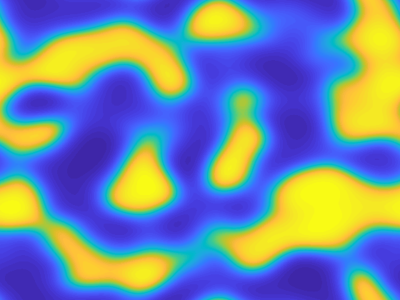
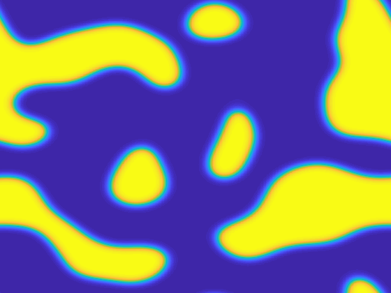
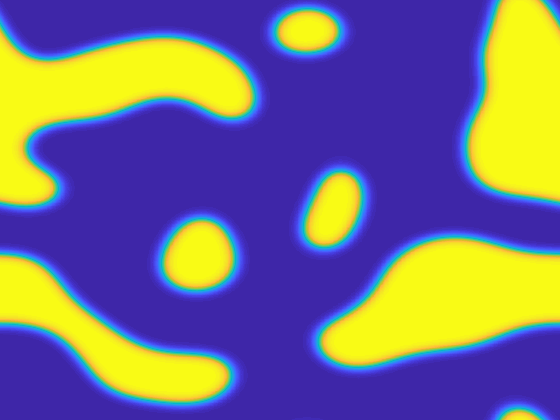
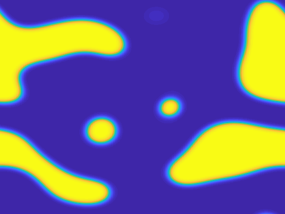
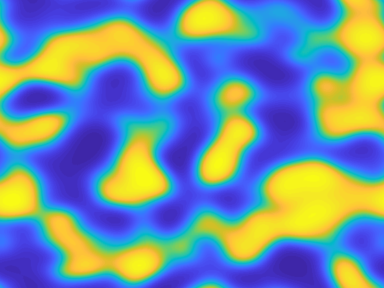
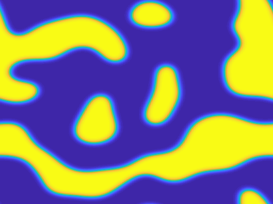
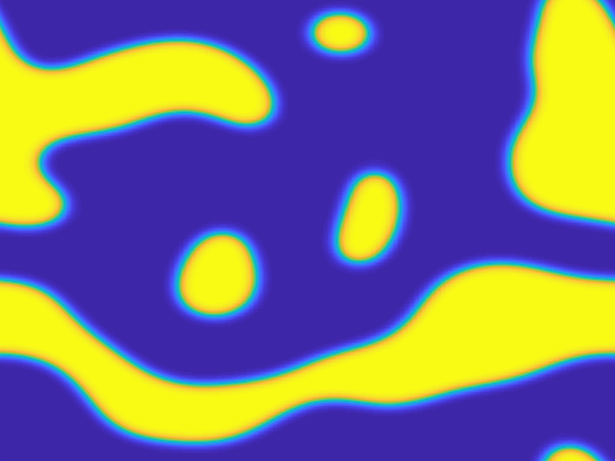
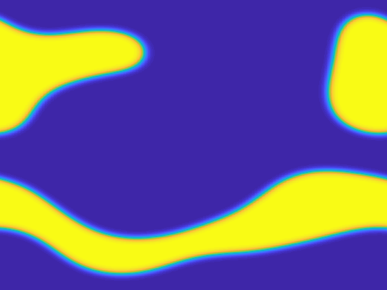
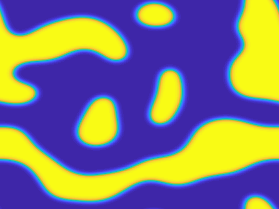
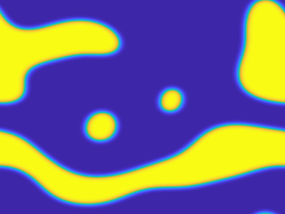
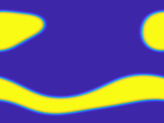
Figure 2: Profiles of coarsening dynamics at $t=10,50,100,300$ (from left to right) with different fractional orders $\alpha=0.4,0.7,0.9$ (from top to bottom), respectively.

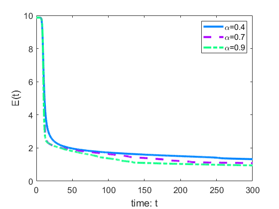
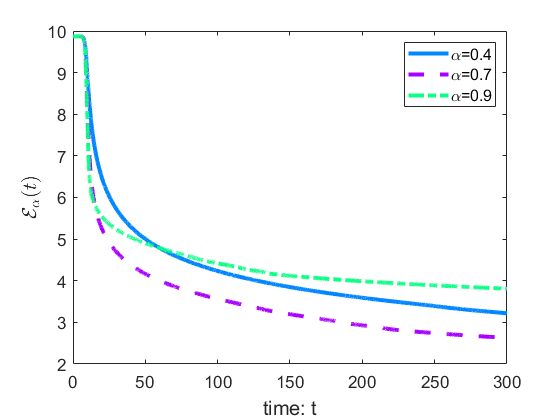
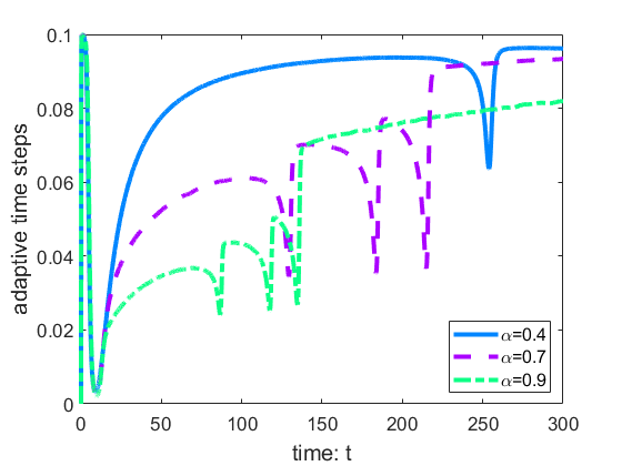
Figure 3: $E(t)$, $\mathcal{E}_{\alpha}(t)$ and adaptive time steps in the coarsening dynamics with the difference fractional orders $\alpha=0.4,0.7,0.9$ (from top to bottom), respectively.

Several practical implementations related numerical simulations are listed below. We use $128^{2}$ grids in space to discretize the domain $(0,2\pi)^{2}$. The graded mesh $t_{k}=T_{0}(k/N_{0})^{\gamma}$ with the settings $\gamma=3,N_{0}=30$ and $T_{0}=0.01$ are always applied in the initial part $[0,T_{0}]$, cf. [9, 8]. For the remainder interval, the time steps are selected according to the following adaptive time-stepping strategy [29, 7]

$$\tau_{ada}=\max\Bigg{\{}\tau_{\min},\frac{\tau_{\max}}{\sqrt{1+\eta\big{\|}\partial_{\tau}\phi^{n}\big{\|}^{2}}}\Bigg{\}}.$$

Always, we take $\tau_{\max}=10^{-1},\,\tau_{\min}=10^{-3}$ and the user parameter $\eta=10^{3}$.

The profiles of coarsening dynamics with different fractional orders $\alpha=0.4,0.7$ and 0.9 for the TFAC model are shown in Figure 2. Snapshots are taken at time $t=10,50,100$ and 300, respectively. We observe that the coarsening rates are dependent on the fractional order and the time period. Near the initial time, the small the fractional order $\alpha$, the faster the coarsening dynamics; while the time goes away from the initial time, the small the fractional order $\alpha$, the slower the coarsening dynamics. The calculated energies using the adaptive time steps for the coarsening dynamics in Figure 2 are depicted in Figure 3. We observe that both the original and variational energies decay with respect to time, while the former decays faster for larger $\alpha$.

References

• [1] S. Allen and J. Cahn. A microscopic theory for antiphase boundary motion and its application to antiphase domain coarsening. Acta Metall., 27:1085–1095, 1979.
• [2] K. Cheng, C. Wang, and S. Wise. An energy stable BDF2 Fourier pseudo-spectral numerical scheme for the square phase field crystal equation. Comm. Comput. Phys., 26:1335–1364, 2019.
• [3] Q. Du, J. Yang, and Z. Zhou. Time-fractional Allen-Cahn equations: analysis and numerical methods. J. Sci. Comput., 85, 2020. Doi.org/10.1007/s10915-020-01351-5.
• [4] X. Feng and S. Wise. Analysis of a Darcy–Cahn–Hilliard diffuse interface model for the hele-shaw flow and its fully discrete finite element approximation. SIAM J. Numer. Anal., 50:1320–1343, 2012.
• [5] Y. Gong, J. Zhao, and Q. Wang. Linear second order in time energy stable schemes for hydrodynamic models of binary mixtures based on a spatially pseudospectral approximation. Adv. Comput. Math., 44:1573–1600, 2018.
• [6] Y. Gong, J. Zhao, and Q. Wang. Arbitrarily high-order unconditionally energy stable schemes for thermodynamically consistent gradient flow models. SIAM J. Sci. Comput., 42:B135–B156, 2020.
• [7] J. Huang, C. Yang, and Y. Wei. Parallel energy-stable solver for a coupled Allen–Cahn and Cahn–Hilliard system. SIAM J. Sci. Comput., 42:C294–C312, 2020.
• [8] B. Ji, H.-L. Liao, Y. Gong, and L. Zhang. Adaptive second-order Crank-Nicolson time-stepping schemes for time fractional molecular beam epitaxial growth models. SIAM J. Sci. Comput., 42:B738–B760, 2020.
• [9] B. Ji, H.-L. Liao, and L. Zhang. Simple maximum-principle preserving time-stepping methods for time-fractional Allen-Cahn equation. Adv. Comput. Math., 46, 2020. Doi:10.1007/s10444-020-09782-2.
• [10] S. Jiang, J. Zhang, Z. Qian, and Z. Zhang. Fast evaluation of the Caputo fractional derivative and its applications to fractional diffusion equations. Comm. Comput. Phys., 21:650–678, 2017.
• [11] N. Kopteva. Error analysis of the L1 method on graded and uniform meshes for a fractional-derivative problem in two and three dimensions. Math. Comput., 88:2135–2155, 2019.
• [12] H.-L. Liao, D. Li, and J. Zhang. Sharp error estimate of nonuniform L1 formula for time-fractional reaction-subdiffusion equations. SIAM J. Numer. Anal., 56:1112–1133, 2018.
• [13] H.-L. Liao, W. Mclean, and J. Zhang. A discrete Grönwall inequality with application to numerical schemes for subdiffusion problems. SIAM J. Numer. Anal., 57:218–237, 2019.
• [14] H.-L. Liao, T. Tang, and T. Zhou. An energy stable and maximum bound preserving scheme with variable time steps for time fractional Allen-Cahn equation. arXiv:2012.10740v1, 2020.
• [15] H.-L. Liao, T. Tang, and T. Zhou. Positive definiteness of real quadratic forms resulting from the variable-step approximation of convolution operators. arXiv:2011.13383v1, 2020.
• [16] H.-L. Liao, Y. Yan, and J. Zhang. Unconditional convergence of a fast two-level linearized algorithm for semilinear subdiffusion equations. J. Sci. Comput., 80:1–25, 2019.
• [17] H-L. Liao and Z. Zhang. Analysis of adaptive BDF2 scheme for diffusion equations. Math. Comput., 2020. Doi:10.1090/mcom/3585.
• [18] J. López-Marcos. A difference scheme for a nonlinear partial integr-odifferential equation. SIAM J. Numer. Anal., 27:20–31, 1990.
• [19] C. Quan, T. Tang, and J. Yang. How to define dissipation-preserving energy for time-fractional phase-field equations. CSIAM-AM, 1:478–490, 2020.
• [20] C. Quan, T. Tang, and J. Yang. Numerical energy dissipation for time-fractional phase-field equations. arXiv:2009.06178v1, 2020.
• [21] J. Shen, J. Xu, and J. Yang. The scalar auxiliary variable (SAV) approach for gradient flows. J. Comput. Phys., 353:407–416, 2018.
• [22] J. Shen and X. Yang. Numerical approximations of Allen-Cahn and Cahn-Hilliard equations. Discrete. Contin. Dyn. Sys., 28:1669–1691, 2010.
• [23] M. Stynes, E. O’Riordan, and J. L. Gracia. Error analysis of a finite difference method on graded meshes for a time-fractional diffusion equation. SIAM J. Numer. Anal., 55:1057–1079, 2017.
• [24] T. Tang, H. Yu, and T. Zhou. On energy dissipation theory and numerical stability for time-fractional phase field equations. SIAM J. Sci. Comput., 41:A3757–A3778, 2019.
• [25] T. Wang, B. Guo, and Q. Xu. Fourth-order compact and energy conservative difference schemes for the nonlinear Schrödinger equation in two dimensions. J. Comput. Phys., 243:382 –399, 2013.
• [26] S. Wise, C. Wang, and J. Lowengrub. An energy-stable and convergent finite-difference scheme for the phase field crystal equation. SIAM J. Numer. Anal., 47:2269–2288, 2009.
• [27] C. Xu and T. Tang. Stability analysis of large time-stepping methods for epitaxial growth models. SIAM J. Numer. Anal., 44:1759–1779, 2006.
• [28] J. Xu, Y. Li, S. Wu, and A. Bousquet. On the stability and accuracy of partially and fully implicit schemes for phase field modeling. Comput. Methods Appl. Mech. Eng., 345:826–853, 2019.
• [29] Z. Zhang and Z. Qiao. An adaptive time-stepping strategy for the Cahn-Hilliard equation. Comm. Comput. Phys., 11:1261–1278, 2012.