User Embedding based Neighborhood Aggregation Method
for Inductive Recommendation

Abstract.

We consider the problem of learning latent features (aka embedding) for users and items in a recommendation setting. Given only a user-item interaction graph, the goal is to recommend items for each user. Traditional approaches employ matrix factorization-based collaborative filtering methods. Recent methods using graph convolutional networks (e.g., LightGCN) achieve state-of-the-art performance. They learn both user and item embedding. One major drawback of most existing methods is that they are not inductive; they do not generalize for users and items unseen during training. Besides, existing network models are quite complex, difficult to train and scale. Motivated by LightGCN , we propose a graph convolutional network modeling approach for collaborative filtering (CF-GCN ). We solely learn user embedding and derive item embedding using light variant (CF-LGCN-U ) performing neighborhood aggregation, making it scalable due to reduced model complexity. CF-LGCN-U models naturally possess the inductive capability for new items, and we propose a simple solution to generalize for new users. We show how the proposed models are related to LightGCN . As a by-product, we suggest a simple solution to make LightGCN inductive. We perform comprehensive experiments on several benchmark datasets and demonstrate the capabilities of the proposed approach. Experimental results show that similar or better generalization performance is achievable than the state of the art methods in both transductive and inductive settings.

1. Introduction

Recommender systems design continues to draw the attention of researchers, as new challenges are to be addressed, with more demanding requirements coming due to several factors: (1) users (e.g., personalized recommendation with high quality), (2) problem scale (e.g., number of users and items, rates at which they grow), (3) information available (e.g., history of user-item interactions, the volume of data, lack of side-information) for learning models (Koren et al., 2009; He et al., 2020), and (4) system resources with constraints (e.g., storage cost, and inference speed). Since recommender systems providepersonalized recommendation because of their design, the development of collaborative filtering (CF) methods that make use of each user’s past item interactions to build a model has drawn immense attention for more than a decade. CF methods’ advantage is that they do not require other domain knowledge. Several important contributions (Ekstrand et al., 2011; Chen et al., 2018; Su and Khoshgoftaar, 2009) have been made along dimensions including new modeling approaches (Koren, 2008; Koren et al., 2009; He et al., 2017; He et al., 2018; He et al., 2020), optimization (Takács and Tikk, 2012; Rao et al., 2015; Rendle et al., 2009; Yang et al., 2020), scalability (George and Merugu, 2005; Papadimitriou and Sun, 2008; Karydi and Margaritis, 2016; Ying et al., 2018).

CF methods require only user-item interaction graph to build models. Neighborhood and latent factor modeling methods are two important classes of CF methods (Koren et al., 2009). Neighborhood-based methods essentially work by discovering/computing relations between entities of the same types (e.g., item-item, user-user) and use this information to recommend items for users (Kabbur et al., 2013). Our interest lies in learning latent features (a.k.a. embedding) for users and items. This way, user embedding can be directly compared with item embedding to score each user-item pair. Matrix factorization methods, a popular class of latent factor modeling methods, include Singular Value Decomposition (Golub and Reinsch, 1970), SVD++ (Koren et al., 2009), Alternating Least Squares (ALS) (Takács and Tikk, 2012), Factorization Machines (FM) (Rendle, 2010). With the advent of neural modeling and deep learning methods, building recommender models using deep neural networks (DNN) and graph neural networks (GNN) has been surging. Neural models are very-powerful, and deliver high quality recommendations (He et al., 2017; Dziugaite and Roy, 2015; He and Chua, 2017; He et al., 2018). However, they come with their challenges: high model complexity, training and inference costs, ability to work in the limited transductive setting, etc. See (Zhang et al., 2019; Gao et al., 2020) for more details.

Our focus in this work is to develop CF models using graph neural networks (Kipf and Welling, 2017; Wang et al., 2019; He et al., 2020; Peng and Mine, 2020; Cao et al., 2021) for learning user and item embedding. Graph convolutional networks (GCNs) have been used successfully in applications such as node classification, link prediction, and recommendation. Of particular interest here is to learn GCN models for collaborative filtering, when there is no side-information (e.g., node features, knowledge graphs). Several GCN model-based CF solutions (Wang et al., 2019; He et al., 2020; Peng and Mine, 2020) have been proposed recently. However, all of them have some limitations (e.g., high training cost, inability to handle large scale data, only transductive). We have two important requirements: (1) scale well - in particular when the number of items is large and significantly higher than the number of users; this situation is encountered in many real-world applications, and (2) able to generalize well on unseen users and items during inference, i.e., we need the model to be inductive.

Our work is inspired by a very recently proposed GCN model, LightGCN (He et al., 2020). This important study investigated different aspects of GCNs for CF and proposed a very attractive simple model that delivered state-of-the-art performance on several benchmark datasets. However, it lacks two important requirements mentioned above. For example, LightGCN learns embedding for both users and items. For reasons stated earlier, this model does not scale well, as the number of model parameters is dependent on the number of items. Therefore, it is expensive to train; also, it adds to model storage cost. Furthermore, LightGCN is transductive, as latent features are not available for new users and items during inference. We address these two important issues in this work, thereby expanding the capabilities of LightGCN .

A key contribution is the proposal of a novel graph convolutional network modeling approach for filtering (CF-GCN ), and we investigate several variants within this important class CF-GCN models. The most important one is CF-GCN-U models which learn only user embedding, and its LightGCN variant, CF-LGCN-U (i.e., using only the most important function, neighborhood aggregation). Since CF-LGCN-U models learn only user embedding, they can perform inductive recommendations with new items. However, this still leaves open the question: how to infer embedding for new users?. We suggest a simple but effective solution that answers this question. As a by-product, we also suggest a simple method to make LightGCN inductive. The CF-LGCN-U modeling approach has several advantages. (1) The CF-LGCN-U model has inductive recommendation capability, as it generalizes for users and items unseen during training. (2) It scales well, as the model complexity is dependent only on the number of users. Therefore, it is very useful in applications where the growth rate of the number of items is relatively high. (3) Keeping both inductive and scalability advantages intact, it can achieve comparable or better performance than more complex models.

We suggest a twin-CF-LGCN-U architecture to increase the expressive power of CF-LGCN-U models by learning two sets of user embedding. This helps to get improved performance in some applications, yet keeping the model complexity advantage (with dependency only on the number of users). Furthermore, we show how the CF-LGCN-U model and its counterpart (CF-LGCN-E model that learns only item embedding) are related to LightGCN . Our basic analysis reveals how training the CF-LGCN-U and CF-LGCN-E models have interpretation of learning neighborhood aggregation functions that make use of user-user and item-item similarities like neighborhood-based CF methods.

We conduct comprehensive experiments on several benchmark datasets in both transductive and inductive setting. First, we show that the proposed CF-LGCN-U models achieve comparable or better performance compared to LightGCN and several baselines on benchmark datasets in the transductive setting. Importantly, this is achieved with reduced model complexity, highlighting that further simplification of LightGCN is possible, making it more scalable. Next, we conduct an experiment to demonstrate the inductive recommendation capability of CF-LGCN-U models. Our experimental results show that the performance in the inductive setting is very close to that achievable in the transductive setting.

In Section 2, we introduce notation and problem setting. Background and motivation for our solution are presented in Section 3. Our proposal of CF-GCN architecture and its variants are detailed in Section 4. We present our experimental setting and results in Section 5. This is followed by discussion and suggestions for future work, and related work in Sections 5 and 6. We conclude with important highlights and observations in Section 7.

2. Notation and Problem Setting

Notation. We use $\mathbf{R}\in\{0,1\}^{m\times n}$ to denote user-item interaction graph, where $m$ and $n$ denote the number of users and items respectively. Let $\mathbf{U}\in{\mathcal{R}}^{m\times d}$ and $\mathbf{E}\in{\mathcal{R}}^{n\times d}$ denote user and item embedding matrices. We assume that the embedding dimension (d) is same for users and items. We use superscript to indicate the layer output embedding (e.g., $\mathbf{U}^{(l)}$ and $\mathbf{E}^{(l)}$ for $l^{th}$ layer embedding output of a network) explicitly, wherever needed. Lower-case letter and subscript are used to refer embedding vectors (row vectors of embedding matrices); for example, $\mathbf{u}^{(l)}_{j}$ and $\mathbf{e}^{(l)}_{k}$ would denote embedding vectors of $j^{th}$ user and $k^{th}$ item at the $l^{th}$ layer output.

Problem Setting. We are given only the user to item interaction graph, $\mathbf{R}$. We assume that no side information (e.g., additional graphs encoding item-item or user-user relations, the user or item features) is available. The goal is to learn latent features for users ($\mathbf{U}$) and items ($\mathbf{E}$) such that user-specific relevant recommendation can be made by ranking items using scores computed from embedding vectors (e.g., the inner product of user and item embedding vectors, $\mathbf{Z}=\mathbf{U}\mathbf{E}^{T}$).

Most collaborating filtering methodologies cannot make recommendations for users/items unseen during training because they are transductive. Therefore, their utility is limited. We are interested in designing a graph embedding based inductive recommendation model where we require the model to have the ability to generalize for users/items unseen during training. We assume that some interactions are available for new users/items during inference. Thus, we require an inductive recommendation modeling solution that can infer embedding vectors for new users and items. Moreover, in many practical applications, the number of items, $n$, grows much higher than the number of users, $m$. Therefore, we aim at developing models with reduced model complexity, having complexity independent of the number of items.

3. Background and Motivation

The simplicity and success of the recently proposed LightGCN model (He et al., 2020) for collaborating filtering inspire our work. LightGCN learns latent features (a.k.a. embedding) for users and items using a lightweight graph convolution neural network. We present some background on graph convolutional networks followed by LightGCN . We then make some observations to motivate our work.

Graph Convolutional Networks. A graph convolutional network (Kipf and Welling, 2017) is composed using graph convolutional layers with each layer performing three basic operations: neighborhood aggregation, feature transformation, and non-linear activation. In GCN, $l^{th}$ layer function is defined as:

$$\mathbf{H}^{(l+1)}=\sigma(\mathbf{A}\mathbf{H}^{(l)}\mathbf{W}^{(l)}).$$

It takes the previous layer output ($\mathbf{H}^{(l)})$ as input, transforms using weight matrix ($\mathbf{W}^{(l)})$, performs aggregation using an adjacency matrix ($\mathbf{A}$), and produces output ($\mathbf{H}^{(l+1)}$) via a nonlinear activation function $\sigma(\cdot)$ (e.g., ReLU or Sigmoid). Kipf and Welling (Kipf and Welling, 2017) proposed to use normalized $\mathbf{A}$ defined as: $\tilde{\mathbf{A}}=\mathbf{D}^{-\frac{1}{2}}(\mathbf{I}+\mathbf{A})\mathbf{D}^{-\frac{1}{2}}$ where $\mathbf{D}$ is the diagonal in-degree matrix of $(\mathbf{I}+\mathbf{A})$ and $\mathbf{I}$ helps to include self node representation in the neighborhood aggregation. In node classification tasks, $\mathbf{H}^{(0)}$ comprises of node features and the model weights $\{\mathbf{W}^{(l)}:l=0,\ldots,L\}$ are learned by optimizing an objective function (e.g., cross-entropy loss) using labeled data.

Recommendation Setting. In the basic model with GCN, we use $\mathbf{A}_{CF}=\begin{bmatrix}{\bf 0}&\mathbf{R}\\ \mathbf{R}^{T}&{\bf 0}\end{bmatrix}$ as the graph and $\mathbf{H}^{(l)}=\begin{bmatrix}\mathbf{U}^{(l)}\\ \mathbf{E}^{(l)}\end{bmatrix}$. Note that user and item embedding vectors are available at each layer output, and propagated through multiple layers. Then, user and item embedding (starting with 1-hot representation at the input) are learned with the GCN model weights using a loss function suitable for collaborative filtering. Following LightGCN (He et al., 2020), we use Bayesian personalized ranking (BPR) loss function defined as:

(1) $${\mathcal{L}}=\sum_{i=1}^{m}\sum_{j\in\mathcal{N}_{e}(u_{i})}\sum_{k\in NS_{e}(u_{i})}g(z_{i,j},z_{i,k};\mathbf{H})+\lambda||\mathbf{H}||^{2}$$

where $\mathcal{N}_{e}(u_{i})$ and $NS_{e}(u_{i})$ denote item neighborhood (with interactions) and negative samples (items) of user $u_{i}$. The function $g(\cdot)$ measures degree of violation of positive pairwise score ($z_{i,j}$) higher than negative pairwise score ($z_{i,k}$) and we use $g(z_{i},z_{j})=-\ln\sigma(z_{i,j}-z_{i,k})$ in our experiments. $\lambda$ is weight regularization constant and $||\mathbf{H}||^{2}$ denote L2-norm of embedding and layer weight vectors. We give more details of model training in the experiment section.

LightGCN . LightGCN draws upon the idea of propagating embedding from prior work on neural graph collaborative filtering (NGCF) (Wang et al., 2019). NGCF uses the basic GCN recommendation model explained above except that an additional term involving element-wise (Hadamard) product of user and item embedding is part of neighborhood aggregation. See (Wang et al., 2019) for more details. He et.al. (Wang et al., 2019) empirically showed that feature transformation and non-linear activation operations are unnecessary in NGCF and can even be harmful to the performance. They proposed a simpler GCN architecture (LightGCN ) by keeping only neighborhood aggregation function with the result: $\mathbf{H}^{(l+1)}=\tilde{\mathbf{A}}\mathbf{H}^{(l)},l=1,\ldots,L$. LightGCN fuses these multi-layer outputs as:

(2) $$\mathbf{H}=\sum_{l=0}^{L}\alpha_{l}\mathbf{H}^{(l)}=\sum_{l=0}^{L}\alpha_{l}\tilde{\mathbf{A}}^{l}\mathbf{H}^{(0)}$$

where $\{\alpha_{l}:l=0,\ldots,L\}$ are fusion hyperparameters. It is worth noting that LightGCN does not require $\mathbf{I}$ while using $\tilde{\mathbf{A}}$, as defined by Kipf and Welling (Kipf and Welling, 2017). Also, note that since $\mathbf{R}$ is a bipartite graph, user and item specific in-degree matrices ($\mathbf{D}_{u}$ and $\mathbf{D}_{e}$) are used in pre/post multiplication of $\mathbf{A}$. See LightGCN (He et al., 2020) for more details. In empirical studies, they found that tuning fusion hyperparameters is not necessary and setting equal weights (i.e., simple average) works well. From (2), we see that the only learnable parameters are $\mathbf{H}^{(0)}=\begin{bmatrix}\mathbf{U}^{(0)}\\ \mathbf{E}^{(0)}\end{bmatrix}$. Furthermore, higher order neighborhood aggregation happens through the effective propagation matrix, $\sum_{l=0}^{L}\alpha_{l}\mathbf{A}^{l}$. Experimental results (He et al., 2020) showed state-of-the-art performance achievable by LightGCN on several benchmark datasets.

Motivation. We observe that LightGCN is quite attractive due to its simplicity and ability to give a state-of-the-art performance. However, it still has two drawbacks. Firstly, it is transductive. Therefore, new items, when they arrive, cannot be recommended for existing users. Similarly, recommending existing items to new users is not possible. Secondly, the model complexity of LightGCN is $O((m+n)d)$. Thus, it poses a scalability issue, for example, when the number of items is extremely huge (i.e., $n\gg m$). In many real-world applications, the rate at which the number of items grows is significantly higher compared to users. Thus, our interest lies in answering two key questions:

• RQ1: How do we make GCN models for collaborative filtering (CF-GCN ) scalable, make it independent of the number of items, yet delivering state-of-the-art performance?

• RQ2: How do we make CF-GCN models inductive?

We answer these questions in the next section. As a by-product, we also show how LightGCN can be made inductive.

4. Proposed Solution

We propose a novel graph convolutional network modeling approach for inductive collaborative filtering (CF-GCN ). We present the idea of learning CF-GCN models with only user embedding (termed CF-GCN-U and its light version, CF-LGCN-U ) and infer item embedding. We discuss several CF-GCN model variants that can be useful for different purposes (e.g., increasing the expressive power of models, scenarios where learning item embedding is beneficial). With basic analysis, we show how the proposed models are related to LightGCN . We also show that training these models can be interpreted as learning neighborhood aggregation function using user-user and item-item similarity function like neighborhood-based CF methods. We show how to use the proposed architecture for the inductive recommendation setting. Finally, we also suggest a simple way of making LightGCN inductive.

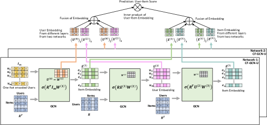
Figure 1. Graph Convolutional Network for Collaborating Filtering Architecture (CF-GCN-U ) with Twin Networks. Each network is CF-GCN-U , using GCN layers with graphs $\mathbf{R}$ and $\mathbf{R}^{T}$. We learn user embedding and derive item embedding. Fuse user and item embedding from different layers/networks. Removing layer weight matrices (except in the first layer) and non-linear activation function $\sigma(\cdot)$ result in the CF-LGCN-U network.

4.1. Collaborating Filtering Networks

The basic idea that we take (Ragesh et al., 2021) is to use heterogeneous graph convolutional layers to compose individual networks and combine embedding outputs from multiple layers and networks. In our setting, since we have only two graphs, $\mathbf{R}$, and $\mathbf{R}^{T}$, there can only be two-layer types. We define UE-GCN layer as the GCN layer that takes item embedding ($\mathbf{E}$) as input and uses $\mathbf{R}$ to produce user embedding ($\mathbf{U}$) output. A similar definition holds for EU-GCN layer.

4.1.1. CF-GCN Networks

A CF-GCN network is composed of a cascaded sequence of UE-GCN and EU-GCN layers. There are only two network types for two reasons: (1) we have only two embedding types (user and item) and start with only one embedding input (i.e., user or item), and (2) we have only two graphs ($\mathbf{R}$ and $\mathbf{R}^{T}$) and layer compatibility (i.e., output and input of two consecutive layers match) is to be ensured. We name these networks, CF-GCN-U and CF-GCN-E , as they take user and item embedding input respectively.

We illustrate with an example. CF-GCN ($\mathbf{R}^{T}$-$\mathbf{R}$-$\mathbf{R}^{T}$) is a three-layer CF-GCN-U network, starting with user embedding input ($\mathbf{U}^{(0)}$). See Figure 1. It produces item embedding outputs, $\mathbf{E}^{(1)}=\sigma(\mathbf{R}^{T}\mathbf{I}_{m}\mathbf{W}^{(1)})$ and $\mathbf{E}^{(3)}=\sigma(\mathbf{R}^{T}\mathbf{U}^{(2)}\mathbf{W}^{(3)})$, as the first and third layer outputs respectively. Note that $\mathbf{U}^{(0)}=\mathbf{W}^{(1)}$ (with 1-hot encoding $\mathbf{I}_{m}$ for users). Further, the network produces user embedding, $\mathbf{U}^{(2)}=\sigma(\mathbf{R}\mathbf{E}^{(1)}\mathbf{W}^{(2)})$, as the second layer output. We fuse $\mathbf{U}^{(0)}$ and $\mathbf{U}^{(2)}$ using AGGREGATION (e.g., mean or weighted sum) or CONCAT functions. Likewise, we obtain a fused item embedding. Finally, we compute each user-item pairwise score, as the inner product of user and item embedding vectors. In this network, the learnable parameters are $\mathbf{U}^{(0)}$ and GCN layer weights ($\mathbf{W}^{(2)}$ and $\mathbf{W}^{(3)})$. Thus, we learn only user embedding, and derive item embedding using this architecture. Likewise, CF-GCN ($\mathbf{R}$-$\mathbf{R}^{T}$-$\mathbf{R}$) is a three layer CF-GCN-E network with learnable $\mathbf{E}^{(0)}$ (only item embedding) and layer weights.

4.1.2. CF-LGCN Networks

As explained earlier, LightGCN uses only neighborhood aggregation and abandons feature and nonlinear transformations. Using this idea, we simplify CF-GCN  networks. Let us continue with the three-layer CF-GCN-U network example. On dropping feature and nonlinear transformation, we get the CF-LGCN-U network with outputs as:

(3) $$\mathbf{E}^{(1)}_{u}=\mathbf{R}^{T}\mathbf{U}^{(0)},\mathbf{E}^{(3)}_{u}=\mathbf{R}^{T}\mathbf{S}_{u}\mathbf{U}^{(0)}$$

(4) $$\mathbf{U}^{(2)}_{u}=\mathbf{S}_{u}\mathbf{U}^{(0)}$$

where $\mathbf{S}_{u}=\mathbf{R}\mathbf{R}^{T}$ measures user-user similarity. Note that we use the subscript $u$ to denote only user embedding model. Using weighted mean with weights $(\alpha_{0},\alpha_{1})$ to fuse, we get:

(5) $$\mathbf{E}_{u}=\mathbf{R}^{T}(\alpha_{0}\mathbf{I}_{m}+\alpha_{1}\mathbf{S}_{u})\mathbf{U}^{(0)}$$

(6) $$\mathbf{U}_{u}=(\alpha_{0}\mathbf{I}_{m}+\alpha_{1}\mathbf{S}_{u})\mathbf{U}^{(0)}.$$

Note that we have used same set of weights (tunable hyperparameters) in (5) and (6) for simplicity, and we can also use layer-wise weights (e.g., ($\alpha_{1}$ and $\alpha_{3}$ in 5) and ($\alpha_{0}$ and $\alpha_{2}$ in 6)). Thus, CF-LGCN-U learns only user embedding, and uses second order user-user information ($\mathbf{S}_{u}$) to infer final user embedding ($\mathbf{U}_{u}$) that captures user-user relation as well. Further, item embedding is inferred by aggregating over its neighbor user embedding (see (5)). It is also useful to note that since $\mathbf{S}_{u}$ is obtained using only $\mathbf{R}$, we have: $\mathbf{R}^{T}\mathbf{S}_{u}=\mathbf{S}_{e}\mathbf{R}^{T}$ where $\mathbf{S}_{e}=\mathbf{R}^{T}\mathbf{R}$. Thus, we can rewrite $\mathbf{E}^{(3)}$ in (3) and $\mathbf{E}_{u}$ in (5) as:

(7) $$\mathbf{E}^{(3)}_{u}=\mathbf{S}_{e}\mathbf{R}^{T}\mathbf{U}^{(0)},\mathbf{E}_{u}=(\alpha_{0}\mathbf{I}_{n}+\alpha_{1}\mathbf{S}_{e})\mathbf{R}^{T}\mathbf{U}^{(0)}.$$

With the definition, ${\hat{\mathbf{E}}^{(0)}_{u}}=\mathbf{R}^{T}\mathbf{U}^{(0)}$, we can interpret ${\hat{\mathbf{E}}^{(0)}_{u}}$ as an effective or proxy item embedding derived from the learned user embedding, with the result: $\mathbf{E}_{u}=\tilde{\mathbf{S}}_{e}{\hat{\mathbf{E}}^{(0)}_{u}}$ where $\tilde{\mathbf{S}}_{e}=(\alpha_{0}\mathbf{I}_{n}+\alpha_{1}\mathbf{S}_{e})$.

It is useful to understand the number of users and item embedding sets we get from a multi-layer network. In one layer case, we have one set of item and user embedding, i.e., $\mathbf{U}^{(0)}$ and $\mathbf{E}^{(1)}$. With two layers, we get two sets of user embedding and one set of item embedding. With three layers, we have two sets each, as seen from (5) and (6). To generalize, we get one set of item embedding lesser with even number of layers. It does not pose any issues in mean fusion. However, when we have even number of layers and use inner product score, we need to drop one set of embedding (either user or item) to ensure dimensions match with concat fusion.

Generalizing (6) and (7) with more layers, fusing with weighted mean and using inner product score ($\mathbf{Z}_{u}=\mathbf{U}_{u}\mathbf{E}^{T}_{u})$, we get the multi-layer CF-LGCN-U network (with $2L+1$ layers) outputs as:

(8) $$\mathbf{E}_{u}=\mathbf{R}^{T}\tilde{\mathbf{S}}_{u}\mathbf{U}^{(0)},\mathbf{U}_{u}=\tilde{\mathbf{S}}_{u}\mathbf{U}^{(0)}$$

(9) $$\mathbf{Z}_{u}=\tilde{\mathbf{S}}_{u}\mathbf{U}^{(0)}(\mathbf{U}^{(0)})^{T}\tilde{\mathbf{S}}^{T}_{u}\mathbf{R}$$

where $\tilde{\mathbf{S}}_{u}=\sum_{l=0}^{L}\alpha_{l}\mathbf{S}^{l}_{u}$, $\mathbf{S}^{0}_{u}=\mathbf{I}_{m}$. Thus, zero and higher powers of user-user and item-item similarities are used with increase in the number of layers. Applying the same steps to the CF-LGCN-E network, we get:

(10) $$\mathbf{E}_{e}=\tilde{\mathbf{S}}_{e}\mathbf{E}^{(0)},\mathbf{U}_{e}=\mathbf{R}\tilde{\mathbf{S}}_{e}\mathbf{E}^{(0)}$$

(11) $$\mathbf{Z}_{e}=\mathbf{R}\tilde{\mathbf{S}}_{e}\mathbf{E}^{(0)}(\mathbf{E}^{(0)})^{T}\tilde{\mathbf{S}}^{T}_{e}$$

where $\tilde{\mathbf{S}}_{e}=\sum_{l=0}^{L}\alpha_{l}\mathbf{S}^{l}_{e}$, $\mathbf{S}^{0}_{e}=\mathbf{I}_{n}$. This network uses only item embedding as denoted by the subscript $e$ and, higher-order similarity information to learn/infer item/user embedding.

4.1.3. Interpretation of CF-LGCN-U and CF-LGCN-E learning

We observe that (9) can be rewritten as: $\mathbf{Z}_{u}=\mathbf{W}_{u}\mathbf{R}$, where $\mathbf{W}_{u}=\tilde{\mathbf{S}}_{u}\mathbf{U}^{(0)}(\mathbf{U}^{(0)})^{T}\tilde{\mathbf{S}}^{T}_{u}$. Thus, we can interpret training as learning user-centric aggregation function (expressed through learnable user embedding, with a special structure), $\mathbf{W}_{u}$, that takes into account the user-user similarity. Likewise, the scoring function with CF-LGCN-E (11) can be rewritten as: $\mathbf{Z}_{e}=\mathbf{R}\mathbf{W}_{e}$, where $\mathbf{W}_{e}=\tilde{\mathbf{S}}_{e}\mathbf{E}^{(0)}(\mathbf{E}^{(0)})^{T}\tilde{\mathbf{S}}^{T}_{e}$. Thus, the score is computed using an item centric transformation (post multiplication) or aggregation function that uses item-item similarity. Thus, CF-LGCN-U and CF-LGCN-E offer learning user and item oriented neighborhood aggregation functions for collaborative filtering.

One natural question is: Which network is better - CF-LGCN-U or CF-LGCN-E ?. We conduct a comparative experimental study later. Note that the number of model parameters is more for CF-LGCN-E when $n>m$. These additional degrees of freedom may help in some applications to get improved performance. However, we emphasize that our interest primarily lies in CF-LGCN-U networks only due to reasons explained earlier. We include CF-LGCN-E discussion to show it as a possible variant within the class of CF-GCN models. Furthermore, it helps to connect CF-GCN modeling approach with LightGCN , as explained below.

4.2. Model Complexity

We observe that the standard GCN model, including LightGCN , uses $\mathbf{A}$ as the adjacency matrix in every GCN layer. Thus, it produces both user and item embedding as each layer output, having $O((m+n)d)$ model complexity. On the other hand, the model complexities of CF-GCN-U and CF-GCN-E networks are $O(md)$ and $O(nd)$ only. Thus, these networks help to reduce model complexity. It is possible to train CF-GCN-U and CF-GCN-E networks jointly, and fuse user/item embedding outputs from both networks. However, this solution has $O((m+n)d)$ complexity. LightGCN is one such solution, as we show next.

4.3. Relation with LightGCN

To understand the relation with LightGCN, we begin with the expression (2) for the embedding vectors, and unfold up to three layers as follows:

(12) $$\mathbf{A}^{2}_{CF}=\begin{bmatrix}\mathbf{S}_{u}&\bf{0}\\ \bf{0}&\mathbf{S}_{e}\end{bmatrix},\mathbf{A}^{3}_{CF}=\begin{bmatrix}\bf{0}&\mathbf{S}_{u}\mathbf{R}\\ \mathbf{S}_{e}\mathbf{R}^{T}&\bf{0}\end{bmatrix}$$

where $\mathbf{S}_{u}=\mathbf{R}\mathbf{R}^{T}$ and $\mathbf{S}_{e}=\mathbf{R}^{T}\mathbf{R}$, and they measure user-user and item-item similarities. Note that while $\mathbf{A}$ is off-block-diagonal, $\mathbf{A}^{2}$ is block-diagonal. Thus, there is a special structure to odd and even powers of $\mathbf{A}$. Using (2) and (12), we get:

(13) $$\mathbf{U}=(\alpha_{0}\mathbf{I}_{m}+\alpha_{2}\mathbf{S}_{u})\mathbf{U}^{(0)}+\mathbf{R}(\alpha_{1}\mathbf{I}_{n}+\alpha_{3}\mathbf{S}_{e})\mathbf{E}^{(0)}$$

(14) $$\mathbf{E}=\mathbf{R}^{T}(\alpha_{1}\mathbf{I}_{m}+\alpha_{3}\mathbf{S}_{u})\mathbf{U}^{(0)}+(\alpha_{0}\mathbf{I}_{n}+\alpha_{2}\mathbf{S}_{e})\mathbf{E}^{(0)}$$

On comparing (13), (14) with three layer embedding outputs of CF-LGCN-U (see (5), (6)) and similar expressions for CF-LGCN-E networks (not shown), we see that LightGCN combines these two network embedding outputs with suitable matching weights. Thus, it makes use of both user-user and item-item second order information in computing user and item embedding. Further, the inner product score computed by LightGCN using (13) and (14) is essentially sum of the CF-LGCN-U and CF-LGCN-E scores (i.e., (9) and (11)); in addition, it has cross-term inner product scores of user embedding of CF-LGCN-U (i.e., the first term in (13)) with item embedding CF-LGCN-E (i.e., the second term in (14)) and vice-versa.

4.4. Twin CF-LGCN-U Networks

As noted earlier, LightGCN uses more parameters and has model complexity $O((m+n)d)$; therefore, more powerful. The question is: can CF-LGCN-U match LightGCN performance with such reduced model complexity?. One simple way to increase the power of CF-LGCN-U is to use two (twin) CF-LGCN-U networks, each learning different sets of user embedding (i.e., $\mathbf{U}^{(0)}_{1}$ and $\mathbf{U}^{(0)}_{2}$). In this case, the effective item embedding of the second network is: $(\mathbf{E}^{(0)}_{u})_{2}=\mathbf{R}^{T}\mathbf{U}^{(0)}_{2}$ and has more degrees of freedom compared to the single CF-LGCN-U network where the effective item embedding is dependent only on $\mathbf{U}^{(0)}$. Note that we can have different number of layers in each network, and the user/item embedding from both networks are fused to get the final user/item embedding. The advantage of the twin CF-LGCN-U network modeling approach is that the model complexity is still independent of the number of items and significant reduction is achieved when $n\gg m$.

The other question is: do we need both networks to get state-of-the-art performance?. In the experiment section, we evaluate different CF-GCN networks on several benchmark datasets. We show that CF-LGCN-U network gives a comparable or better performance than LightGCN through empirical studies. Furthermore, the model complexity is reduced and incurs lesser storage costs when $m<n$.

4.5. Inductive Recommendation

LightGCN is a transductive method because we learn both user/item embedding and it is not apparent how to infer embedding for new users and items. Graph embedding based inductive recommendation model requires the ability to infer new user and item embedding. Using CF-LGCN networks which learn only user embedding meets this requirement as discussed below. We present our solution starting with the easier problem of fixed user set with training data available to learn user embedding and we need to generalize only for new items. Then, we expand the scope to include new users and suggest a simple solution for CF-LGCN-U networks. Also, as a by-product, we show how LightGCN can be modified for making inductive inference.

4.5.1. Inductive CF-LGCN-U : Only New Items

Let us consider the three-layer CF-LGCN-U example again (see (3) - (7)). Since we learn only user embedding and infer item embedding, CF-LGCN-U can infer embedding for new items. Let $\mathbf{R}_{I}$ denote new user-item interaction graph such that new items (i.e., new columns) are also appended. We assume that at least a few interactions are available for each new item in $\mathbf{R}_{I}$. In practice, this is possible because one can record interactions on new items shown to randomly picked or targeted existing users. Recall that the three-layer CF-LGCN-U network uses $\mathbf{R}^{T}-\mathbf{R}-\mathbf{R}^{T}$ in tandem. We compute new item embedding by substituting $\mathbf{R}_{I}$ for $\mathbf{R}$ in each layer. Note that we can choose to use $\mathbf{R}$ or $\mathbf{R}_{I}$ in the second layer (i.e., to compute fresh user embedding or not). We conduct an ablation study to evaluate the efficacy of using fresh user embedding and present our results shortly.

4.5.2. Inductive CF-LGCN-U : New Users

Since we learn user embedding in CF-LGCN-U , we face the same question of how to infer embedding for new users?. When we look at (5) and (6) closely, the main difficulty arises from the term $\alpha_{0}\mathbf{I}_{m}\mathbf{U}^{(0)}$, as we cannot get embedding for new users without retraining. We propose a naive solution to address this problem. Suppose we set $\alpha_{0}=0$, that is, we do not use $\mathbf{U}^{(0)}$ in the fusion step. We can then still compute fresh user embedding by substituting new $\mathbf{R}_{U}$ (i.e., $\mathbf{R}$ with added rows) in the second layer. However, the number of user embedding sets available for fusion is lesser by one set. Since the inner product of fused user and item embedding requires that the dimensions match, we also drop the first layer item embedding output and add one more layer, if needed, to ensure a valid CONCAT fusion. This simple solution provides the ability to infer new user embedding, and we demonstrate its usefulness through empirical studies.

4.5.3. Inductive CF-LGCN-U : New Users and Items

We handle both new users/items’ by not using embedding outputs of the first layer (i.e., by setting $\alpha_{0}=0$ for the user and item embedding, as needed). Note that we update both user and item embedding. This update requires using $\mathbf{R}_{I}$ (i.e., ignoring new users) in the first layer and fully updated, $\mathbf{R}$ (i.e., having both new users and items) in other layers.. It is important to keep in mind that we require at least a few labeled entries for new users/items during inductive inference. Finally, we note that the idea of not using the first layer user embedding is useful for LightGCN . Our experimental results show that inductive LightGCN also works.

5. Experiments

We first discuss experimental setup, including a brief description of the datasets and introduces the baselines used; this sub-section also covers the training details, metrics and hyperparameter optimization. We evaluate our proposed approach in both Transductive and Inductive settings, present and discuss our results.

5.1. Experimental Setup

5.1.1. Datasets

We used the three datasets provided in the LightGCN repository (a) Gowalla (Liang et al., 2016) contains the user location check-in data (b) Yelp2018 (Wang et al., 2019) contains local business (treated as item) recommendation to users (c) Amazon-book (He and McAuley, 2016) contains book recommendation to users. We include one additional dataset Douban-Movie (Zheng et al., 2017) to our evaluation; this dataset consists of user-movie interactions. The statistics of datasets are detailed in the table 1.

5.1.2. Transductive Dataset Preparation

As the repository only contained train and test splits, we sampled 10% of items randomly for each user from the train split to construct the validation split. As there is a difference in the splits used in LightGCN, we retrain all the baselines on these new splits and report the metrics.

5.1.3. Inductive Dataset Preparation

In the inductive setting, we do not have access to all the users or items during the training process. New users/items can arrive post the model training, with new user-item interactions. Given these interactions, we need to derive embeddings for these new items/users without retraining. To evaluate in this setting, we hold out 5% of users and items randomly (with a minimum of 10 and 5 interactions respectively) and remove them from the train, validation and test splits in the transductive setting. At the time of inference, we assume we have access to a partial set of interactions involving all the new users and new items using which we derive their embeddings. We then evaluate the model on the rest of the interactions, along with the test set.

Dataset	User #	Item #	Interaction #
Gowalla	29, 858	40, 981	1, 027, 370
Yelp2018	31, 668	38, 048	1, 561, 406
Amazon-Book	52, 643	91, 599	2, 984, 108
Douban-movie	3, 022	6, 971	195, 472

Table 1. Statistics of benchmark datasets

5.1.4. Methods of comparison

LightGCN gives a state-of-the-art performance. Hence LightGCN forms the primary baseline against which we compare all our proposed models. Additionally, we have included the following baselines.

MF (Rendle et al., 2011): This is the traditional matrix factorization model that does not utilize the graph information directly.
NGCF (Wang et al., 2019): Neural Graph Collaborative Filtering is a graph neural network based model that captures high-order information by embedding propagation using graphs. We utilized the code from this repository to obtain performance metrics.
Mult-VAE (Liang et al., 2018): This is a collaborative filtering method based on variational autoencoder. We run the code released by the authors after modifying it to run on the train/val/test splits of our other experiments.
GRMF-Norm (Rao et al., 2015): Graph Regularized Matrix Factroiation additonally adds a graph Laplacian regularizer in addition to the MF objective. We used the GRMF-Norm variant as described in (He et al., 2020)
GCN: This baseline is equivalent to the non-linear version of LightGCN with transformation matrices learnt as is done in the traditional GCN layers.

5.1.5. Training Details

We implemented all the above methods except NGCF and Mult-VAE. The training pipeline is setup identical to that of LightGCN for a fair comparison. We use BPR  (Rendle et al., 2009) based loss function to train all the models using Adam Optimizer (Kingma and Ba, 2015). All the models were trained for at most 1000 epochs with validation recall@20 evaluated every 20 epochs. There is early stopping when there is no improvement in the metric for ten consecutive evaluations. Additionally, we conducted all our experiments in a distributed setting, training on 4 GPU nodes using Horovod (Sergeev and Balso, 2018). All the models we implemented are PyTorch based. We fixed embedding size to 64 for all the models. And the batch sizes for all datasets were fixed to 2048 except for Amazon-Book for which was set to 8192. Learning rate was swept over {1e-1, 1e-2, 5e-3, 1e-3, 5e-4}, embedding regularization over {1e-2, 1e-3, 1e-4, 1e-5, 1e-6}, graph dropout over {0.0, 0.1, 0.2, 0.25}. Additionally for NGCF, node dropout was swept over {0.0, 0.1, 0.2, 0.25} and the coefficient for graph laplacian regularizer for GRMF-Norm was swept over {1e-2, 1e-3, 1e-4, 1e-5, 1e-6}. We tuned the hyperparameters dropout rate in the range $[0,0.2,0.5]$, and $\beta$ in $[0.2,0.4,0.6,0.8]$ for Mult-VAE with the model architecture as $200\rightarrow 600\rightarrow 200$, and the learning rate as 1e-3. For the proposed model, we also varied graph normalization as hyperparameters.

5.2. Transductive Setting Experiments

We carried out a detailed experimental study with the proposed CF-LGCN variants. We show the usefulness of twin networks first. Then, we present results with multiple layers and layer combination. We compare the recommended variants (CF-LGCN-U ) of our proposed approach to the state-of-the-art baselines.

5.2.1. Single CF-LGCN-U network Versus Twin CF-LGCN-U network

In Table 2, we present results obtained from evaluating single CF-LGCN-U network and twin CF-LGCN-U network on four benchmark datasets. We used three layers in each network. Recall that we learn two sets of user embedding with the twin network. We see that the twin CF-LGCN-U network performs better than the single CF-LGCN-U network on all datasets except Yelp2018. The results show that the twin CF-LGCN-U network is beneficial, and can achieve higher performances by increasing the expressive power of CF-LGCN-U network. Hence, we use only the twin network in the rest of our experiments. Performance on Yelp2018 suggests that even a single network is sufficient in some application scenario. Therefore, it helps to experiment with both models and perform model section using the validation set.

Recall / NDCG @ 20	Gowalla	Yelp2018	Amazon-Book	Douban-Movie
CF-LGCN-U	16.81 / 14.35	6.41 / 5.30	4.48 / 3.51	4.85 / 3.51
Twin CF-LGCN-U	17.02 / 14.45	6.36 / 5.24	4.52 / 3.59	5.23 / 3.28

Table 2. Twin CF-LGCN-U vs CF-LGCN-U

5.2.2. Experiment with Multiple Layers

In this experiment, we study the usefulness of having multiple layers in twin CF-LGCN-U network. From Table 4, we see that increasing the number of layers improves the performance significantly on Yelp2018 and Amazon-Book datasets. This result demonstrates the usefulness of higher-order information available through propagation. The performance starts saturating, for example, in the Gowalla dataset. Besides, it is useful to note that increasing the number of layers beyond a certain limit may hurt the performance due to over-smoothing, as reported in node classification tasks (Kipf and Welling, 2017). Therefore, it is crucial to treat layer size as a model hyperparameter and tune using validation set performance.

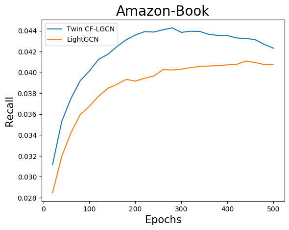
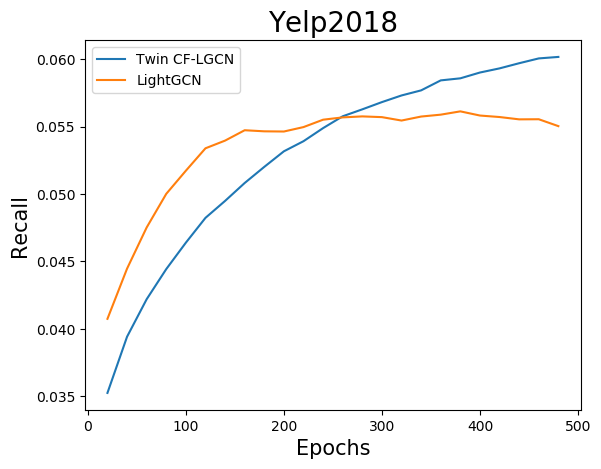
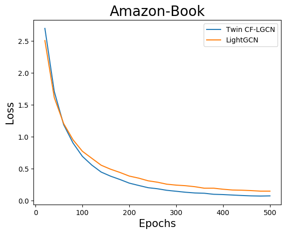
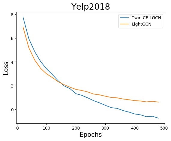
Figure 2. Training loss and Test Recall @20 metric as as function of epochs

5.2.3. Effect of Fusion

LightGCN reported that fusing embedding output from different layers helps to get improved performance compared to using only the final layer embedding output, and we observed a similar phenomenon in our experiments. We tried two variants of fusion: Mean and Concat. Following LightGCN , we used uniform weighting with Mean. From Table 3, we see that Concat fusion delivers significant improvement with our twin CF-LGCN-U network model. Therefore, we use Concat fusion with our model in rest of the experiments. Note that fusion can be done in several other ways, particularly when working with two networks. We leave this exercise for future experimental studies.

5.2.4. Comparison with Baselines

We performed a detailed experimental study by comparing the proposed model with several state-of-the-art baselines.In Figure 2, we compare the training loss and recall$@$20 of the proposed twin CF-LGCN-U model with LightGCN on the Amazon-Book and Yelp2018 datasets. Detailed results are presented in Table 4. We observe that the 3-layers twin CF-LGCN-U network model performs uniformly better than the strongest competitor, LightGCN , except on the Gowalla dataset where the performance is very close. Thus, the proposed model is quite competitive to LightGCN and is a powerful alternative to LightGCN . As explained earlier, the CF-LGCN-U network has the advantage of learning only user embedding. From Table 1, we see that the number of items is higher than the number of users, and is nearly twice for the Amazon-Book and Douban-Movie datasets. Thus, the proposed CF-LGCN-U network can deliver similar or better performance than LightGCN with significantly reduced complexity, enabling large scale learning.

Recall / NDCG @ 20	Aggregation	Gowalla	Yelp2018	Amazon-Book	Douban-Movie
Twin CF-LGCN-U (2L)	Mean	16.38 / 13.76	6.48 / 5.35	4.17 / 3.31	5.15 / 3.22
Twin CF-LGCN-U (2L)	Concat	17.09 / 14.51	6.31 / 5.19	4.32 / 3.44	5.17 / 3.23
Twin CF-LGCN-U (3L)	Mean	16.71 / 14.27	6.06 / 5.03	4.24 / 3.31	5.16 / 3.17
Twin CF-LGCN-U (3L)	Concat	17.02 / 14.45	6.36 / 5.24	4.52 / 3.59	5.23 / 3.28

Table 3. Different Layerwise Fusion

Recall / NDCG @ 20	Gowalla	Yelp2018	Amazon-Book	Douban-Movie
MF	14.55 / 11.56	5.17 / 4.16	3.49 / 2.67	4.24 / 2.77
NGCF	15.69 / 12.82	5.60 / 4.55	3.85 / 2.94	4.85 / 3.00
Mult-VAE	13.65 / 10.10	5.74 / 4.40	3.94 / 2.97	4.85 / 3.00
GRMF-Norm	15.65 / 13.12	5.60 / 4.61	3.50 / 2.71	4.78 / 3.00
GCN (3L)	16.10 / 13.76	6.14 / 5.06	3.67 / 2.84	4.78 / 3.02
LightGCN (1L)	17.11 / 14.59	6.17 / 5.04	3.76 / 2.93	4.75 / 3.03
LightGCN (2L)	16.70 / 14.27	6.12 / 4.97	3.99 / 3.08	4.71 / 2.98
LightGCN (3L)	17.21 / 14.65	6.07 / 5.00	4.10 / 3.16	4.95 / 3.14
Twin CF-LGCN-U (1L)	17.08 / 14.48	6.20 / 5.13	3.87 / 3.07	4.91 / 3.19
Twin CF-LGCN-U (2L)	17.09 / 14.51	6.31 / 5.19	4.32 / 3.44	5.17 / 3.23
Twin CF-LGCN-U (3L)	17.02 / 14.45	6.36 / 5.24	4.52 / 3.59	5.23 / 3.28

Table 4. Comparison with Baselines

5.2.5. Twin CF-LGCN-U vs Twin CF-LGCN-E

Our CF-GCN network architecture supports another variant CF-LGCN-E . Though our interest primarily lies in CF-LGCN-U , we compare these two variants. In Table 5, we report results from this experiment. We see that the twin CF-LGCN-U network outperforms its counter-part twin CF-LGCN-E on all datasets except the Douban-Movie dataset where the performance is very close. Note that the number of model parameters is significantly higher in the CF-LGCN-E network, as $n>m$. Nevertheless, the performance is inferior. There has always been this question of developing user-centric versus item-centric models (Koren, 2008) and studying this problem using CF-GCN models is beyond the scope of this work. We leave this study for the future.

Recall / NDCG @ 20	Gowalla	Yelp2018	Amazon-Book	Douban-Movie
Twin CF-LGCN-U	17.02 / 14.45	6.36 / 5.24	4.52 / 3.59	5.23 / 3.28
Twin CF-LGCN-E	15.36 / 12.60	6.16 / 5.03	4.27 / 3.36	5.28 / 3.39

Table 5. Twin CF-LGCN-U vs Twin CF-LGCN-E

5.3. Inductive Setting Experiments

5.3.1. Generalization to New Items and New Users

We carried out a detailed experimental study to evaluate the effectiveness of inductive variants of CF-LGCN-U and LightGCN . We report three sets of metrics for both these models.
Inductive: This is a standard inductive setup where several users and items are unseen during training. During inference, we use partial interactions available for all the new entities to obtain their embeddings. Note that we do not need to retrain these models.
Transductive (Upper Bound): In this setup, we train the model along with the partial interactions, thereby having access to all the users and items during training. The motivation to report these numbers is to get an upper bound on the performance.
Transductive (Lower Bound): This set of numbers indicates the lower bound and highlights the performance gain that one can achieve by recommending for new users and items. Training and inference are made exactly like the inductive setting. However, we assume that we cannot make recommendations for new users and new items during the evaluation.

From the results in Table 6, the inductive variants of both CF-LGCN-U and LightGCN obtain significant gains over the corresponding Transductive (Lower Bound) metrics and closer to the Transductive (Upper Bound) metrics. This result indicates that the proposed inductive modification is quite effective in generalizing to new users and items. CF-LGCN-U performs better than LightGCN on Yelp2018 and Amazon-Book datasets, while it is marginally inferior in the Gowalla dataset (as was observed in the transductive setting).

5.3.2. Effect of Updating User Embedding

Additionally, we carried out a few experiments in a setting where we had access to all the users during training and evaluated the performance only on new items. As we have access to all the user embedding, we only need to derive embedding for new items. We can derive item embedding while retaining the user embedding as it is, or we could update the embedding for users as well when we get access to the partial interactions for the new items. We report metrics for both these cases in Table 7. As we can see, updating user embedding with partially observed interactions during inference can be very useful over using static user embedding.

Recall / NDCG @ 20	Gowalla	Yelp2018	Amazon-Book
Transductive (Lower Bound)
LightGCN	15.58 / 12.60	5.79 / 4.87	3.66 / 2.94
Twin CF-LGCN-U	14.49 / 12.49	5.78 / 4.92	4.02 / 3.29
Inductive
LightGCN	16.79 / 14.80	6.38 / 5.58	4.28 / 3.69
Twin CF-LGCN-U	16.71 / 14.68	6.44 / 5.69	4.88 / 4.26
Transductive (Upper Bound)
LightGCN	17.19 / 15.34	6.44 / 5.65	4.59 / 3.98
Twin CF-LGCN-U	17.09 / 15.11	6.48 / 5.71	5.11 / 4.49

Table 6. Generalization to New Users and New Items

Recall / NDCG @ 20	Gowalla	Yelp2018	Amazon-Book
Twin CF-LGCN-U (2L)	16.12 / 13.72	6.11 / 5.19	4.08 / 3.33
Twin CF-LGCN-U (2L) with U+	16.68 / 14.45	6.23 / 5.29	4.23 / 3.48

Table 7. U+ suffix represents the model for which we update user embedding during inference

6. Related Work

Recommendation problems are ubiquitous in our day-to-day life. User-Item interaction graphs capture historical information on users interaction with various items. Collaborative Filtering (CF) methods utilize these interaction graphs to make item recommendations to users. User-item interactions have several dimensions:
1. Binary / Real Valued: Interactions could be binary (e.g. user bought a product or not) or real-valued (e.g. user gave a 5/10 rating on a video). This distinction might seem trivial; however, there are several subtle differences between the two. In binary interaction graphs, we are often interested in predicting top-k items for a user; hence, the interest metric is often NDCG@k. In real-valued interactions like ratings, we are interested in predicting user’s rating for an item (regardless of the user’s preference towards that item). Thereby, the metric often measured here is the MSE. Also, there are inherent biases involved in real-valued interactions - a user may be prone to giving high ratings to all products, or a popular item is prone to receiving high ratings. Such biases are absent in a binary interaction graph.
2. Explicit / Implicit: Interactions could be explicit (e.g. user purchased a product) or implicit (e.g. user watched a YouTube video). Explicit feedbacks create a reliable user-interaction graph which can lead to a reliable recommendation. If a user purchases an item, we can be sure that they liked/sought the item. Hence, recommendations learnt from such graphs have a high degree of confidence in being liked/sought by the user. However, implicit feedback, due to its nature, creates a highly unreliable graph. Just because a user watched a YouTube video does not imply that the user liked it. Any recommendation made on such unreliable information can be noisy.

Several methods have been proposed for CF over the years, addressing different aspects of the recommendation problem.
Factorization Methods: Early methods assumed fixed user and item set, and proposed Matrix Factorization (MF) based methods (Golub and Reinsch, 1970; Koren et al., 2009; Takács and Tikk, 2012) which treats the user-item interaction graph as a matrix. These methods can successfully handle binary interactions. For real-valued interactions, addressing inherent biases is essential. (Koren, 2008) computes explicit per-user per-item bias estimates to get improved performance. In cases of implicit interactions, it is necessary to identify meaningful interactions for downstream recommendation problems; hence attention-based models have been developed for such scenarios that use side-information to model attention (Chen et al., 2017; He et al., 2018). With the advent of deep learning, non-linear models of matrix factorization have been proposed (He et al., 2017) and models that can leverage rich side information to get improved recommendation (Wang et al., 2015; Zhang et al., 2016). AutoEncoder-based models (Wu et al., 2016; Liang et al., 2018) have been proposed to address implicit interactions.
GNN based:Viewing graphs as matrices has certain inherent limitations. Since not all users interact with all items, certain entries in the matrix are missing. Replacing them with default values addresses these missing entry problems. Choice of the default value often dictates the performance of the model. Additionally, these methods do not explicitly exploit the collaborative nature of the user-item interaction graph. Researchers have started to look at Graph Neural Networks (GNNs) (Wu et al., 2019) to circumvent these issues. Graph Convolutional Network (GCN) (Kipf and Welling, 2017), a particular instantiation of GNNs, has shown to be capable of exploiting graphs to give improved performance. (van den Berg et al., 2017) adapt GCNs for user-item interaction graph and show that it can improve performance over baseline MF methods; however, it only uses single-hop information. (Wang et al., 2019) adapts the model to incorporate multiple hop information. (Ying et al., 2018) developed a random walk based GCN model that can work for a massive graph. (He et al., 2020) proposed a simplified version of the GCN where neighborhood aggregation alone gave good gains.
Inductive: All the above methods, however, assume a fixed user-item set. This assumption can be very restrictive, particularly in social network and e-commerce scenarios where several new users and new items get added every day. In such cases, it is desirable to have an inductive method which does not assume a fixed user-item set. Our proposed approach is one such method. In this approach, we derive item embeddings from user-embeddings and user-embeddings can be derived from item-embeddings. Exploiting such relationship allows the model to generalize to new users and new items without retraining. Our proposed approach is competitive with existing approaches in transductive settings, showing that it is possible to express item-embeddings in terms of user-embeddings and vice versa. It also performs well in inductive settings without degradation, proving its generalizability to new users and new items. There have been a few prior works in inductive recommendation (Hartford et al., 2018; Zhang and Chen, 2020). However, these methods work on real-valued interaction graphs. As discussed earlier, the real-valued interactions have implicit biases. These are either addressed by either estimating per user, per item bias as done in (Koren, 2008) or modeling each real-valued possibility as a separate relation as done in (Zhang and Chen, 2020). Addressing these biases is a non-trivial problem and beyond the scope of the work. We refrain from comparing with these approaches as we restrict our focus to binary-valued user-item interaction graphs.

7. Discussion and Future Work

We focused our attention on applying the proposed modeling approach to scenarios where user-interaction data is available as binary information and user-specific recommendation is made, with recommendation quality measured using metrics such as recall$@k$ and ndcg$@k$. Learning models in this application setting comes with several other important factors, including negative sampling (Yang et al., 2020) and choice of loss functions (e.g., approximate ndcg (Bruch et al., 2019)) that help to get improved performance. Incorporating these factors and conducting an experimental study is beyond the scope of this work.

Another important recommendation application is rating prediction task (e.g., users rating movies or products) (Koren et al., 2009). Several methods have been developed and studied recently. This includes graph neural networks based matrix completion (van den Berg et al., 2017; Zhang and Chen, 2020), heterogeneous (graph) information networks (Shi et al., 2019) which uses concepts such as meta-path where a meta-path (e.g., User - Book - Author - Book) encodes semantic information with higher order relations. Further, several solutions to address cold-start (e.g., recommending for users/items having only a few rating entries) and inductive inference (Zhang and Chen, 2020). In some application setting, knowledge graphs (e.g., explicit user-user relational graphs) are available, and they are used to improve the recommendation quality. See (Gao et al., 2020) for more details.

We can adapt our CF-GCN modeling approach for these different application scenarios by modifying network architecture, for example, using GCN with additional graph types (Ragesh et al., 2021), relational GCN (R-GCN) (Tian et al., 2020), Reco-GCN (Xu et al., 2019)) and optimizing for metrics such as mean-squared-error (MSE), mean-absolute error (MAE) and ndcg$@k$ etc. We leave all these directions for future work.

8. Conclusion

We consider the problem of learning graph embedding based method for collaborative filtering (CF). We set out to develop an inductive recommendation model with graph neural networks and build scalable models that have reduced model complexity. We proposed a novel graph convolutional networks modeling approach for collaborating (CF-GCN ). Among the possible variants within this approach’s scope, our primary candidate is the CF-LGCN-U network and its twin variant. The CF-LGCN-U network model learns only user embedding. This network offers inductive recommendation capability, therefore, generalizes for users and items unseen during training. Furthermore, its model complexity is dependent only on the number of users. Thus, its model complexity is significantly lesser compared to even light models such as LightGCN . CF-LGCN-U models are quite attractive in many practical application scenarios, where the number of items is significantly lesser than the number of users. We showed the relation between the proposed models and LightGCN . Our experimental results demonstrate the efficacy of the proposed modeling approach in both transductive and inductive settings.

References

- (1)
- Bruch et al. (2019) Sebastian Bruch, Masrour Zoghi, Michael Bendersky, and Marc Najork. 2019. Revisiting Approximate Metric Optimization in the Age of Deep Neural Networks. In Proceedings of the 42nd International ACM SIGIR Conference on Research and Development in Information Retrieval (Paris, France) (SIGIR’19). Association for Computing Machinery, New York, NY, USA, 1241–1244.
- Cao et al. (2021) Jiangxia Cao, Xixun Lin, Shu Guo, Luchen Liu, Tingwen Liu, and Bin Wang. 2021. Bipartite Graph Embedding via Mutual Information Maximization. In WSDM.
- Chen et al. (2017) Jingyuan Chen, Hanwang Zhang, Xiangnan He, Liqiang Nie, Wei Liu, and Tat-Seng Chua. 2017. Attentive Collaborative Filtering: Multimedia Recommendation with Item- and Component-Level Attention. In Proceedings of the 40th International ACM SIGIR Conference on Research and Development in Information Retrieval.
- Chen et al. (2018) R. Chen, Q. Hua, Y. Chang, B. Wang, L. Zhang, and X. Kong. 2018. A Survey of Collaborative Filtering-Based Recommender Systems: From Traditional Methods to Hybrid Methods Based on Social Networks. IEEE Access 6 (2018), 64301–64320.
- Dziugaite and Roy (2015) Gintare Karolina Dziugaite and Daniel M. Roy. 2015. Neural Network Matrix Factorization. CoRR abs/1511.06443 (2015). arXiv:1511.06443
- Ekstrand et al. (2011) Michael D. Ekstrand, John T. Riedl, and Joseph A. Konstan. 2011. Collaborative Filtering Recommender Systems. Found. Trends Hum.-Comput. Interact. 4, 2 (Feb. 2011), 81–173.
- Gao et al. (2020) Yang Gao, Yi-Fan Li, Yu Lin, Hang Gao, and Latifur Khan. 2020. Deep Learning on Knowledge Graph for Recommender System: A Survey. arXiv:2004.00387 [cs.IR]
- George and Merugu (2005) T. George and S. Merugu. 2005. A scalable collaborative filtering framework based on co-clustering. In Fifth IEEE International Conference on Data Mining (ICDM’05).
- Golub and Reinsch (1970) G. H. Golub and C. Reinsch. 1970. Singular Value Decomposition and Least Squares Solutions. Numer. Math. 14, 5 (April 1970), 403–420.
- Hartford et al. (2018) Jason Hartford, Devon Graham, Kevin Leyton-Brown, and Siamak Ravanbakhsh. 2018. Deep Models of Interactions Across Sets. In Proceedings of the 35th International Conference on Machine Learning (Proceedings of Machine Learning Research, Vol. 80), Jennifer Dy and Andreas Krause (Eds.). PMLR, Stockholmsmässan, Stockholm Sweden, 1909–1918.
- He and McAuley (2016) Ruining He and Julian J. McAuley. 2016. Ups and Downs: Modeling the Visual Evolution of Fashion Trends with One-Class Collaborative Filtering. (2016).
- He and Chua (2017) Xiangnan He and Tat-Seng Chua. 2017. Neural Factorization Machines for Sparse Predictive Analytics. In Proceedings of the 40th International ACM SIGIR Conference on Research and Development in Information Retrieval (Shinjuku, Tokyo, Japan) (SIGIR ’17). Association for Computing Machinery, New York, NY, USA.
- He et al. (2020) Xiangnan He, Kuan Deng, Xiang Wang, Yan Li, YongDong Zhang, and Meng Wang. 2020. LightGCN: Simplifying and Powering Graph Convolution Network for Recommendation. Association for Computing Machinery, New York, NY, USA, 639–648.
- He et al. (2018) X. He, Z. He, J. Song, Z. Liu, Y. Jiang, and T. Chua. 2018. NAIS: Neural Attentive Item Similarity Model for Recommendation. IEEE Transactions on Knowledge and Data Engineering 30, 12 (2018), 2354–2366.
- He et al. (2017) Xiangnan He, Lizi Liao, Hanwang Zhang, Liqiang Nie, Xia Hu, and Tat-Seng Chua. 2017. Neural Collaborative Filtering (WWW ’17). International World Wide Web Conferences Steering Committee, Republic and Canton of Geneva, CHE.
- Kabbur et al. (2013) Santosh Kabbur, Xia Ning, and George Karypis. 2013. FISM: Factored Item Similarity Models for Top-N Recommender Systems. In Proceedings of the 19th ACM SIGKDD.
- Karydi and Margaritis (2016) Efthalia Karydi and Konstantinos Margaritis. 2016. Parallel and Distributed Collaborative Filtering: A Survey. ACM Comput. Surv. 49, 2, Article 37 (Aug. 2016), 41 pages.
- Kingma and Ba (2015) Diederik P. Kingma and Jimmy Ba. 2015. Adam: A Method for Stochastic Optimization. In ICLR.
- Kipf and Welling (2017) Thomas N. Kipf and Max Welling. 2017. Semi-Supervised Classification with Graph Convolutional Networks. In ICLR.
- Koren (2008) Yehuda Koren. 2008. Factorization Meets the Neighborhood: A Multifaceted Collaborative Filtering Model. In Proceedings of the 14th ACM SIGKDD. Association for Computing Machinery, New York, NY, USA.
- Koren et al. (2009) Y. Koren, R. Bell, and C. Volinsky. 2009. Matrix Factorization Techniques for Recommender Systems. Computer 42, 8 (2009), 30–37.
- Liang et al. (2016) Dawen Liang, Laurent Charlin, James McInerney, and David M. Blei. 2016. Modeling User Exposure in Recommendation. In Proceedings of the 25th International Conference on World Wide Web (Montréal, Québec, Canada) (WWW ’16). International World Wide Web Conferences Steering Committee, Republic and Canton of Geneva, CHE, 951–961.
- Liang et al. (2018) Dawen Liang, Rahul G. Krishnan, Matthew D. Hoffman, and Tony Jebara. 2018. Variational Autoencoders for Collaborative Filtering. In Proceedings of the 2018 World Wide Web Conference.
- Papadimitriou and Sun (2008) S. Papadimitriou and J. Sun. 2008. DisCo: Distributed Co-clustering with Map-Reduce: A Case Study towards Petabyte-Scale End-to-End Mining. In 2008 Eighth IEEE International Conference on Data Mining.
- Peng and Mine (2020) Shaowen Peng and Tsunenori Mine. 2020. A Robust Hierarchical Graph Convolutional Network Model for Collaborative Filtering. arXiv:2004.14734 [cs.IR]
- Ragesh et al. (2021) Rahul Ragesh, Sundararajan Sellamanickam, Arun Iyer, Ram Bairi, and Vijay Lingam. 2021. HeteGCN: Heterogeneous Graph Convolutional Networks for Text Classification. In WSDM.
- Rao et al. (2015) Nikhil Rao, Hsiang-Fu Yu, Pradeep Ravikumar, and Inderjit S. Dhillon. 2015. Collaborative Filtering with Graph Information: Consistency and Scalable Methods. In Advances in Neural Information Processing Systems 28: Annual Conference on Neural Information Processing Systems 2015, December 7-12, 2015, Montreal, Quebec, Canada, Corinna Cortes, Neil D. Lawrence, Daniel D. Lee, Masashi Sugiyama, and Roman Garnett (Eds.). 2107–2115.
- Rendle (2010) S. Rendle. 2010. Factorization Machines. In 2010 IEEE International Conference on Data Mining. 995–1000.
- Rendle et al. (2009) Steffen Rendle, Christoph Freudenthaler, Zeno Gantner, and Lars Schmidt-Thieme. 2009. BPR: Bayesian Personalized Ranking from Implicit Feedback. In Proceedings of the Twenty-Fifth Conference on Uncertainty in Artificial Intelligence (Montreal, Quebec, Canada) (UAI ’09). AUAI Press, Arlington, Virginia, USA, 452–461.
- Rendle et al. (2011) Steffen Rendle, Zeno Gantner, Christoph Freudenthaler, and Lars Schmidt-Thieme. 2011. Fast Context-Aware Recommendations with Factorization Machines. In Proceedings of the 34th International ACM SIGIR Conference on Research and Development in Information Retrieval (Beijing, China) (SIGIR ’11). Association for Computing Machinery, New York, NY, USA, 635–644.
- Sergeev and Balso (2018) Alexander Sergeev and Mike Del Balso. 2018. Horovod: fast and easy distributed deep learning in TensorFlow. CoRR abs/1802.05799 (2018).
- Shi et al. (2019) C. Shi, B. Hu, W. X. Zhao, and P. S. Yu. 2019. Heterogeneous Information Network Embedding for Recommendation. IEEE Transactions on Knowledge and Data Engineering 31, 2 (2019), 357–370.
- Su and Khoshgoftaar (2009) Xiaoyuan Su and Taghi M. Khoshgoftaar. 2009. A Survey of Collaborative Filtering Techniques. Adv. in Artif. Intell. 2009, Article 4 (Jan. 2009), 1 pages.
- Takács and Tikk (2012) Gábor Takács and Domonkos Tikk. 2012. Alternating Least Squares for Personalized Ranking. In Proceedings of the Sixth ACM Conference on Recommender Systems (Dublin, Ireland) (RecSys ’12). Association for Computing Machinery, New York, NY, USA, 83–90.
- Tian et al. (2020) Anqi Tian, Chunhong Zhang, Miao Rang, Xueying Yang, and Zhiqiang Zhan. 2020. RA-GCN: Relational Aggregation Graph Convolutional Network for Knowledge Graph Completion. In Proceedings of the 2020 12th International Conference on Machine Learning and Computing (Shenzhen, China) (ICMLC 2020). Association for Computing Machinery, New York, NY, USA, 580–586.
- van den Berg et al. (2017) Rianne van den Berg, Thomas N. Kipf, and Max Welling. 2017. Graph Convolutional Matrix Completion. CoRR abs/1706.02263 (2017). arXiv:1706.02263
- Wang et al. (2015) Hao Wang, Naiyan Wang, and Dit-Yan Yeung. 2015. Collaborative Deep Learning for Recommender Systems. In Proceedings of the 21th ACM SIGKDD International Conference on Knowledge Discovery and Data Mining (Sydney, NSW, Australia) (KDD ’15). Association for Computing Machinery, New York, NY, USA, 1235–1244.
- Wang et al. (2019) Xiang Wang, Xiangnan He, Meng Wang, Fuli Feng, and Tat-Seng Chua. 2019. Neural Graph Collaborative Filtering. In Proceedings of the 42nd International ACM SIGIR Conference on Research and Development in Information Retrieval (Paris, France) (SIGIR’19). Association for Computing Machinery, New York, NY, USA, 165–174.
- Wu et al. (2016) Yao Wu, Christopher DuBois, Alice X. Zheng, and Martin Ester. 2016. Collaborative Denoising Auto-Encoders for Top-N Recommender Systems. In Proceedings of the Ninth ACM International Conference on Web Search and Data Mining.
- Wu et al. (2019) Zonghan Wu, Shirui Pan, Fengwen Chen, Guodong Long, Chengqi Zhang, and Philip S. Yu. 2019. A Comprehensive Survey on Graph Neural Networks. ArXiv abs/1901.00596 (2019).
- Xu et al. (2019) Fengli Xu, Jianxun Lian, Zhenyu Han, Yong Li, Yujian Xu, and Xing Xie. 2019. Relation-Aware Graph Convolutional Networks for Agent-Initiated Social E-Commerce Recommendation. In Proceedings of the 28th ACM CIKM.
- Yang et al. (2020) Zhen Yang, Ming Ding, Chang Zhou, Hongxia Yang, Jingren Zhou, and Jie Tang. 2020. Understanding Negative Sampling in Graph Representation Learning. 1666–1676.
- Ying et al. (2018) Rex Ying, Ruining He, Kaifeng Chen, Pong Eksombatchai, William L. Hamilton, and Jure Leskovec. 2018. Graph Convolutional Neural Networks for Web-Scale Recommender Systems. In KDD.
- Zhang et al. (2016) Fuzheng Zhang, Nicholas Jing Yuan, Defu Lian, Xing Xie, and Wei-Ying Ma. 2016. Collaborative Knowledge Base Embedding for Recommender Systems. In Proceedings of the 22nd ACM SIGKDD International Conference on Knowledge Discovery and Data Mining (San Francisco, California, USA) (KDD ’16). Association for Computing Machinery, New York, NY, USA, 353–362.
- Zhang and Chen (2020) Muhan Zhang and Yixin Chen. 2020. Inductive Matrix Completion Based on Graph Neural Networks. In ICLR.
- Zhang et al. (2019) Shuai Zhang, Lina Yao, Aixin Sun, and Yi Tay. 2019. Deep Learning Based Recommender System: A Survey and New Perspectives. ACM Comput. Surv. 52, 1, Article 5 (Feb. 2019), 38 pages.
- Zheng et al. (2017) Jing Zheng, Jian Liu, Chuan Shi, Fuzhen Zhuang, Jingzhi Li, and Bin Wu. 2017. Recommendation in heterogeneous information network via dual similarity regularization. International Journal of Data Science and Analytics 3 (02 2017).