Learning Accurate Decision Trees with Bandit Feedback via Quantized Gradient Descent

Abstract

Decision trees provide a rich family of highly non-linear but efficient models, due to which they continue to be the go-to family of predictive models by practitioners across domains. But learning trees is challenging due to their discrete decision boundaries. The state-of-the-art (SOTA) techniques resort to (a) learning soft trees thereby losing logarithmic inference time; or (b) using methods tailored to specific supervised learning settings, requiring access to labeled examples and loss function. In this work, by leveraging techniques like overparameterization and straight-through estimators, we propose a unified method that enables accurate end-to-end gradient based tree training and can be deployed in a variety of settings like offline supervised learning and online learning with bandit feedback. Using extensive validation on standard benchmarks, we demonstrate that our method provides best of both worlds, i.e., it is competitive to, and in some cases more accurate than methods designed specifically for the supervised settings; and in bandit settings, where most existing tree learning techniques are not applicable, our models are still accurate and significantly outperform the applicable SOTA methods.

1 Introduction

Decision trees are an important and rich class of non-linear ML models, often deployed in practical machine learning systems for their efficiency and low inference cost. They can capture fairly complex decision boundaries and are state-of-the-art (SOTA) in several application domains. Optimally learning trees is a challenging discrete, non-differentiable problem that has been studied for several decades and is still receiving active interest from the community (Gouk et al., 2019; Hazimeh et al., 2020; Zantedeschi et al., 2021).

Most of the existing literature studies tree learning in the context of traditional supervised settings like classification (Carreira-Perpinán and Tavallali, 2018) and regression (Zharmagambetov and Carreira-Perpinan, 2020), where the methods require access to explicit labeled examples and full access to a loss function. However, in several scenarios we might not have access to labeled examples, and the only supervision available might be in the form of evaluation of the loss/reward function at a given point. One such scenario is the “bandit feedback” setting, that often arises in real-world ML systems (e.g., recommender systems with click-feedback), where the feedback for the deployed model is in the form of loss/reward. The bandit setting has been long-studied both in the theoretical/optimization communities as well as in the ML community (Dani et al., 2008; Dudík et al., 2011; Agarwal et al., 2014; Shamir, 2017). The Vowpal Wabbit (VW) library is extensively used by practitioners for solving learning problems in this setting.

So, in this work, we address the question: can we design a general method for training hard decision trees, that works well in the standard supervised learning setting, as well as in settings with limited supervision? In particular, we focus on online bandit feedback in the presence of context. Here, at each round the learner observes a context/example, picks an action/prediction either from a discrete space (classification) or continuous space (regression) for which it then receives a loss, which must be minimized. Since the structure of this loss function is unknown to the learner, it is referred to as black-box loss, in contrast to the loss observed in the supervised setting where the entire structure is known to the learner. Notice that this loss function can be evaluated only once for an example. Hereafter, we will refer to this setting in the paper simply as the bandit setting or the bandit feedback setting.

Recently, several neural techniques have been proposed to improve accuracy of tree methods by training with differentiable models. However, either their (Yang et al., 2018; Lee and Jaakkola, 2020) accuracies do not match the SOTA tree learning methods on baseline supervised learning tasks or they end up with “soft” decision trees (Irsoy et al., 2012; Frosst and Hinton, 2017; Biau et al., 2019; Tanno et al., 2019; Popov et al., 2020) which is not desirable for practical settings where inference cost may be critical. Using annealing techniques to harden the trees heavily compromises on the accuracy (as seen in Section 5). On the other hand, there is a clear trade-off between softness (and in turn inference cost) and performance in SOTA tree methods (Hazimeh et al., 2020) which try to minimize the number of leaves reached per example (Section 5).

SOTA (hard) tree learning methods (Carreira-Perpinán and Tavallali, 2018; Hehn et al., 2019; Zharmagambetov and Carreira-Perpinan, 2020), based on alternating optimization techniques, yield impressive performance in the batch/fully supervised setting (as seen in Section 5), but their applicability drastically diminishes in more general bandit settings where the goal is to achieve small regret with few queries to the loss function. It is unclear how to extend such methods to bandit settings, as these methods optimize over different parameters alternatively, thus requiring access to multiple loss function evaluations per point.

We propose a simple, end-to-end gradient-based method “Dense Gradient Trees” (DGT) that gives best of both worlds — (1) logarithmic inference cost, (2) significantly more accurate and sample-efficient than general methods for online settings, (3) competitive to SOTA tree learning methods designed specifically for supervised tasks, and (4) easily extensible to ensembles that outperform widely-used choices by practitioners. DGT appeals to the basic definition of the tree function that involves a product over hard decisions at each node along root-to-leaf paths, and $\arg\max$ over paths. We make three key observations regarding the tree function and re-formulate the learning problem by leveraging successful techniques from deep networks training literature: 1) the path computation And function can be expressed in “sum of decisions” form rather than the multiplicative form which has ill-conditioned gradients, 2) we can overparameterize the tree model via learning a linear deep embedding of the data points without sacrificing efficiency or the tree structure, and 3) hard decisions at the nodes can be enforced using quantization-aware gradient updates.

The reformulated tree learning problem admits efficient computation of dense gradients with respect to model parameters leveraging quantization-aware (noisy) gradient descent and gradient estimation via perturbation. We provide algorithms for standard supervised learning (DGT) and bandit (DGT-Bandit) settings, and extensively evaluate them on multiple classification and regression benchmarks, in supervised as well as in bandit settings. On supervised tasks, DGT achieves SOTA accuracy on most of the datasets, comparing favorably to methods designed specifically for the tasks. In the bandit setting, DGT-Bandit achieves up to 30% less regret than the SOTA method for classification and up to 50% less regret than the applicable baseline for regression.

Our key contributions are: 1) A unified and differentiable solution for learning decision trees accurately for practical and standard evaluation settings, 2) competitive (or superior) performance compared to SOTA hard decision tree learning methods on a variety of datasets, across different problem settings, and 3) enabling sample-efficient tree learning in the online, bandit feedback setting without exact information on the loss function or labels.

1.1 Related Work

Several lines of research focus on different aspects of the tree learning problem, including shallow and sparse trees (Kumar et al., 2017), efficient inference (Jose et al., 2013), and incremental tree learning in streaming scenarios (Domingos and Hulten, 2000; Jin and Agrawal, 2003; Manapragada et al., 2018; Das et al., 2019) (where labels are given but arrive online). The most relevant ones are highlighted below.

Non-greedy techniques: “Tree Alternating Optimization” (TAO) is a recent SOTA non-greedy technique for learning classification (Carreira-Perpinán and Tavallali, 2018) and regression (Zharmagambetov and Carreira-Perpinan, 2020) trees. It updates the nodes at a given height (in parallel) using the examples routed to them in the forward pass while keeping the nodes in other heights fixed. The gradients during backpropagation are “sparse” in that each example contributes to $O(h)$ updates. This poses a challenge from a sample complexity perspective in the online setting. In contrast, DGT performs “dense” gradient updates, i.e., with one example’s one (quantized) forward pass, $O(2^{h})$ model parameters can be updated in our backpropagation. Interestingly, we find DGT achieves competitive results to TAO even in the batch setting (see Section 5). Norouzi et al. (2015) optimizes a (loose) relaxation of the empirical loss; it requires $O(h)$ loss evaluations per example (as against just 1 in DGT) to perform gradient update, so it does not apply to bandit settings. Bertsimas and Dunn (2017); Bertsimas et al. (2019) formulate tree learning as a mixed integer linear program (ILP) but their applicability is limited in terms of problem settings and scale. LCN (Lee and Jaakkola, 2020) uses $h$-layer ReLU networks to learn oblique trees of height $h$. But, for a given height, their model class admits only a subset of all possible trees which seems to deteriorate its performance (see Section 5).

Soft trees/Neural techniques: Several, mostly neural, techniques (Jordan and Jacobs, 1994; Irsoy et al., 2012; Kontschieder et al., 2015; Balestriero, 2017; Frosst and Hinton, 2017; Biau et al., 2019; Tanno et al., 2019; Popov et al., 2020) try to increase the accuracy of decision trees by resorting to soft decisions and/or complex internal nodes and end up producing models that do not have oblique tree structure (Definition 1). The recently proposed (Zantedeschi et al., 2021) embeds trees as layers of deep neural networks, and relaxes mixed ILP formulation to allow optimizing the parameters through a novel “argmin differentiation” method. In Jordan and Jacobs (1994); Irsoy et al. (2012); Frosst and Hinton (2017), all root-to-leaf path probabilities have to be computed for a given example, and the output is a weighted sum of decisions of all paths. Two recent tree learning methods are notable exceptions: 1) Hehn et al. (2019) uses an E-M algorithm with sigmoid activation and annealing to learn (hard) trees, and 2) TEL (Hazimeh et al., 2020) is a novel smooth-step activation function-based method that yields a small number of reachable leaves at the end of training, often much smaller than $O(2^{h})$ for probabilistic trees. However, the inference cost of the method is relatively much larger than ours, to achieve competitive accuracy, as we show in Section 5.3.

Bandit feedback: Contextual bandit algorithms for this setting allow general reward/loss functions but are mostly applicable to discrete output domains like classification (Agarwal et al. (2014)); e.g.  Féraud et al. (2016) learns an axis-aligned decision tree/forest on discretized input features, and Elmachtoub et al. (2017) learns a separate decision tree for every action via bootstrapping. In contrast, DGT uses noisy gradient estimation techniques (Flaxman et al., 2005; Agarwal et al., 2010) (together with our tree learning reformulation) to provide an accurate solution for both bandit classification and regression settings.

2 Problem Setup

Denote data points by $\mathbf{x}\in\mathbb{R}^{d}$. In this work, we focus on learning oblique binary decision trees.

Definition 1 (Oblique binary decision tree).

An oblique binary tree of height $h$ represents a piece-wise constant function $f(\mathbf{x};\mathbf{W},\boldsymbol{\Theta}):\mathbb{R}^{d}\to\mathbb{R}^{K}$ parameterized by weights $\mathbf{w}_{ij}\in\mathbb{R}^{d},b_{ij}\in\mathbb{R}$ at $(i,j)$-th node ($j$-th node at depth $i$) computing decisions of the form $\langle\mathbf{w}_{ij},\mathbf{x}\rangle+b_{ij}>0$, that decide whether $\mathbf{x}$ must traverse the left or right child next. For classification, we associate parameters $\boldsymbol{\theta}_{j}\in\mathbb{R}^{K}$ at $j$-th leaf node, encoding scores or probabilities for each of the $K$ classes. For regression, $\theta_{j}\in\mathbb{R}$ $(K=1)$ is the prediction given by the $j$-th leaf node.

We devise algorithms for learning tree model parameters $(\mathbf{W},\boldsymbol{\Theta})$ in two different settings.
(I) Contextual Bandit setting. In many practical settings, e.g. when ML models are deployed in online systems, the learner gets to observe the features $\mathbf{x}_{i}$ but may not have access to label information; the learner only observes a loss (or reward) value for its prediction on $\mathbf{x}_{i}$. We have zeroth-order access to $\ell:f(\mathbf{x}_{i};\mathbf{W},\boldsymbol{\Theta})\to\mathbb{R}_{+}$, i.e. $\ell$ is an unknown loss function that can only be queried at a given point ($\mathbf{W}_{i},\boldsymbol{\Theta}_{i}$). The goal then is to minimize the regret:

$$\frac{1}{n}\sum_{i=1}^{n}\ell\big{(}f(\mathbf{x}_{i};\mathbf{W}_{i},\boldsymbol{\Theta}_{i})\big{)}-\min_{\mathbf{W},\boldsymbol{\Theta}}\ \frac{1}{n}\sum_{i=1}^{n}\ell\big{(}f(\mathbf{x}_{i};\mathbf{W},\boldsymbol{\Theta})\big{)}.$$

(II) Supervised learning. This is the standard setting in which, given labeled training data $(\mathbf{x}_{i},y_{i})_{i=1}^{n}$, where $y_{i}$ is the label of $\mathbf{x}_{i}$, and a known loss $\ell:\big{(}f(\mathbf{x};\mathbf{W},\boldsymbol{\Theta}),y\big{)}\to\mathbb{R}_{+}$, the goal is to learn a decision tree that minimizes empirical loss on training data:

$$\min_{\mathbf{W},\boldsymbol{\Theta}}\ \ \ \ \frac{1}{n}\sum_{i=1}^{n}\ell\big{(}f(\mathbf{x}_{i};\mathbf{W},\boldsymbol{\Theta}),y_{i}\big{)}+\lambda\Phi_{\text{reg}}(\mathbf{W},\boldsymbol{\Theta}),$$ (1)

where $\Phi_{\text{reg}}(.)$ is a suitable regularizer for model parameters, and $\lambda>0$ is the regularization parameter. We consider both regression (with squared loss) and classification (with multiclass 0-1 loss).

Our method DGT (Section 4) provides an end-to-end gradient of tree prediction with respect to the tree parameters, so we can combine the tree with any other network (i.e., allow $f\big{(}g(\mathbf{x});\mathbf{W},\boldsymbol{\Theta}\big{)}$, where $g$ and $\boldsymbol{\Theta}$ can be neural networks) or loss function, and will still be able to define the backpropagation for training the tree. So, in addition to the above loss functions and supervised learning setting, DGT readily applies to a more general set of problems like multi-instance learning (Dietterich et al., 1997), semi-supervised learning (Van Engelen and Hoos, 2020), and unsupervised learning (Chapter 14, Friedman et al. (2001)). We also consider a forest version of DGT (called DGT-Forest) in Section 5.

Notation: Lowercase bold letters $\mathbf{x},\mathbf{w},$ etc. denote column vectors. Uppercase bold letters (e.g. $\mathbf{W},\boldsymbol{\Theta}$) denote model parameters. $\mathbf{x}(i),\mathbf{w}(j)$ denote the $i$-th and the $j$-th coordinate of $\mathbf{x}$ and $\mathbf{w}$, respectively.

3 Our Tree Learning Formulation

Learning decision trees is known to be NP-hard (Sieling, 2003) due to the highly discrete and non-differentiable optimization problem. SOTA methods typically learn the tree greedily (Breiman et al., 1984; Quinlan, 2014) or using alternating optimization at multiple depths of the tree (Carreira-Perpinán and Tavallali, 2018; Zharmagambetov and Carreira-Perpinan, 2020). These methods typically require full access to the loss function (see Related Work for details). We remedy this concern by introducing a simple technique that allows end-to-end computation of the gradient of all tree parameters. To this end, we first introduce a novel flexible re-formulation of the standard tree learning problem; in Section 4, we utilize the re-formulation to present efficient and accurate learning algorithms in both bandit and supervised (batch) settings.

Consider a tree of height $h$. Let $I(i,l)$ denote the index of the $l$-th leaf’s predecessor in the $i$-th level of the tree; e.g., for all $i$, $I(i,l)=0$ if $l$ is the left-most leaf node. Also, define $S(i,l)$ as:

$$S(i,l)=\begin{cases}-1,\ \text{ if }l\text{-th leaf}\in\text{left subtree of node }I(i,l),\\ +1,\ \ \text{ otherwise}.\end{cases}$$

Recall that $\mathbf{w}_{ij}\in\mathbb{R}^{d}$ and $b_{ij}\in\mathbb{R}$ are the weights and bias of the node $j$ at depth $i<h$, and $\boldsymbol{\theta}_{l}$ are the parameters at leaf $l$. Now, the decision $f(\mathbf{x};\mathbf{W},\boldsymbol{\Theta})$ can be written as:

$$f(\mathbf{x};\mathbf{W},\boldsymbol{\Theta}) =\sum_{l=0}^{2^{h}-1}q_{l}(\mathbf{x};\mathbf{W})\boldsymbol{\theta}_{l},\text{where}$$ (2)

$$q_{l}(\mathbf{x};\mathbf{W}) =\prod_{i=0}^{h-1}\sigma\bigg{(}\big{(}\langle\mathbf{w}_{i,I(i,l)},\mathbf{x}\rangle+b_{i,I(i,l)}\big{)}S(i,l)\bigg{)}.$$

In decision trees, $\sigma(.)$ is the step function, i.e.,

$$\sigma_{\text{step}}(a)=1,\ \text{if}\ a\geq 0,\text{ and }\ \sigma_{\text{step}}(a)=0,\ \text{if}\ a<0.$$ (3)

This hard thresholding $\sigma_{\text{step}}$ presents a key challenge in learning the tree model. A standard approach is to relax $\sigma_{\text{step}}$ via, say, the sigmoid function (Sethi, 1990; Kumar et al., 2017; Biau et al., 2019), and model the tree function as a distribution over the leaf values. Though this readily enables learning via gradient descent-style algorithms, the resulting model is not a decision tree as the decision at each node is soft thus leading to exponential (in height) inference complexity. Also, using standard methods like annealing to convert the soft decisions into hard decisions leads to a significant drop in accuracy (see Table 1).

Applying standard gradient descent algorithm to solve (1) has other potential issues besides the hard/soft decision choices with the choice of $\sigma$. In the following, we leverage three simple but key observations to model the function $f$ in (2), which lets us design efficient and accurate algorithms for solving (1) with any general, potentially unknown, loss function $\ell$.

3.1 AND gradients

The $q_{l}$ function (2) to compute the And of the decisions along a root-to-leaf path has a multiplicative form, which is commonly used in tree learning formulations (Kumar et al., 2017). When we use the relaxed sigmoid function for $\sigma$, this form implies that the gradient and the Hessian of the function with respect to the parameters are highly ill-conditioned (multiplication of $h$ sigmoids). That is, in certain directions, the Hessian values can be vanishingly small, while others will have a scale of $O(1)$. It is hard to reconcile the disparate scales of the gradient values, leading to poor solutions which we observe empirically as well (in Section 5). We leverage a simple but key observation that $q_{l}$ can be equivalently written using a sum instead of the multiplicative form:

$$\small{q_{l}(\mathbf{x};\mathbf{W})=\sigma\big{(}\sum_{i=0}^{h-1}\sigma\big{(}\big{(}\langle\mathbf{w}_{i,I(i,l)},\mathbf{x}\rangle+b_{i,I(i,l)}\big{)}S(i,l)\big{)}-h\big{)}.}$$ (4)

Proposition 1.

The path function $q$ in (4) is identical to the definition in (2), when $\sigma:=\sigma_{\text{step}}$ in (3).

The proposition follows directly from the definition of $\sigma_{\text{step}}$ : $q_{l}$ term in Eqn. (2) evaluates to 1 iff all terms in the product evaluate to 1 (corresponding to the decisions made along the root-to-leaf path); Similarly in Eqn. (4) (which operates on the same terms as that of $q_{l}$ in Eqn. (2)) evaluates to 1 iff each term in the sum is 1, because the sum will then be $h$, which after the offset $-h$ yields 1 according to the definition of $\sigma_{\text{step}}$. Therefore the two definitions of $q_{l}$ are equivalent.

The gradient of $q_{l}$ in (4) is a sum of $h$ terms each of which is a product of only two sigmoids, so the problem should be much better conditioned. Our hypothesis is validated empirically in Section 5.

3.2 Overparameterization

Overparameterization across multiple layers is known to be an effective tool in deep learning with strong empirical and theoretical results (Allen-Zhu et al., 2019; Arora et al., 2019; Sankararaman et al., 2020), and is hypothesized to provide a strong regularization effect. While large height decision trees can seem “deep” and overparameterized, they do not share some of the advantages of deep overparameterized networks. In fact, deeper trees seem to be harder to train, tend to overfit and provide poor accuracy.

So in this work, we propose overparameterizing by learning “deep” representation of the data point itself, before it is being fed to the decision tree. That is, we introduce $L$ linear fully-connected hidden layers with weights $\mathbf{W}^{(1)}\in\mathbb{R}^{d_{1}\times d},\mathbf{W}^{(2)}\in\mathbb{R}^{d_{2}\times d_{1}},\dots,{\color[rgb]{0,0,0}\mathbf{W}^{(L-1)}}\in\mathbb{R}^{{\color[rgb]{0,0,0}d_{L-1}}\times d_{L-2}},{\color[rgb]{0,0,0}\mathbf{W}^{(L)}}\in\mathbb{R}^{{\color[rgb]{0,0,0}2^{h}-1}\times d_{L-1}}$, where $d_{i}$ are hyper-parameters, and apply tree function $f$ to $f(\mathbf{W}^{(L-1)}\mathbf{W}^{(L-2)}\dots\mathbf{W}^{(1)}\mathbf{x};\mathbf{W}^{{\color[rgb]{0,0,0}(L)}},\boldsymbol{\Theta})$. Note that $L$ is the number of hidden layers we use for our overparameterization.

Note that while we introduce many more parameters in the model, due to linearity of the network, each node still has a linear decision function: $\langle\mathbf{w}_{ij}^{{\color[rgb]{0,0,0}(L)}},\mathbf{W}^{(L-1)}\mathbf{W}^{(L-2)}\dots\mathbf{W}^{(1)}\mathbf{x}\rangle=\langle\widetilde{\mathbf{w}}_{ij},\mathbf{x}\rangle$ where $\widetilde{\mathbf{w}}_{ij}={\color[rgb]{0,0,0}(\mathbf{W}^{(L-1)}\mathbf{W}^{(L-2)}\dots\mathbf{W}^{(1)})^{\top}\mathbf{w}_{ij}^{{\color[rgb]{0,0,0}(L)}}}$. Thus, we still learn an oblique decision tree (Def. 1) and do not require any feature transformation during inference.

Remark 1.

We emphasize that despite using overparameterization, we finally obtain standard oblique decision tree (Definition 1) with a linear model at each internal node. In particular, we do not require any feature transformation at the inference time, unlike the tree learning approaches of Kontschieder et al. (2015); Tanno et al. (2019) that learn deep representations thereby increasing the model size and inference time.

Given that linear overparameterization works with exactly the same model class, it is surprising that the addition of linear layers yields significant accuracy improvements in several datasets (Section 5.4). Indeed, there are some theoretical studies (Arora et al., 2018) on why linear networks might accelerate optimization, but we leave a thorough investigation into the surprising effectiveness of linear overparameterization for future work.

3.3 Quantization for hard decisions

As mentioned earlier, for training, a common approach is to replace the hard $\sigma_{\text{step}}$ with the smooth sigmoid, and then slowly anneal the sigmoid to go towards sharper decisions (Jose et al., 2013; Kumar et al., 2017). That is, start with a small scaling parameter $s$ in sigmoid function $\sigma_{s}(a):=\frac{1}{1+\exp(-s\ \cdot\ a)}$, and then slowly increase the value of $s$. We can try to devise a careful annealing schedule of increasing values of $s$, but the real issue in such a training procedure is that it cannot output a hard tree in the end — we still need to resort to heuristics to convert the converged model to a tree, and the resulting loss in accuracy can be steep (see Table 1).

Instead, we use techniques from the quantization-aware neural network literature (Rastegari et al., 2016; Courbariaux et al., 2016; Hubara et al., 2016; Esser et al., 2020), which uses the following trick: apply quantized functions in the forward pass, but use smooth activation function in the backward pass to propagate appropriate gradients. In particular, we leverage the scaled quantizers and the popular “straight-through estimator" to compute the gradient of the hard $\sigma_{\text{step}}$ function (Rastegari et al., 2016; Courbariaux et al., 2016) (discussed in Section 4). Note that, unlike typical quantized neural network scenarios, our setting requires (1-bit) quantization of only the $\sigma$ functions.

Finally, using the aforementioned three ideas, we reformulate the tree learning problem (1) as:

$$\min_{\mathbf{W}^{(m)},\boldsymbol{\Theta}}\frac{1}{n}\sum_{i=1}^{n}\ell\big{(}f(\mathbf{x}_{i};\mathbf{W},\boldsymbol{\Theta}),y_{i}\big{)}+\lambda\Phi_{\text{reg}}(\mathbf{W},\boldsymbol{\Theta}),$$ (5)

$$\ \ \ \text{s.t. }\ \ \mathbf{W}=\mathbf{W}^{(L)}\mathbf{W}^{(L-1)}\dots\mathbf{W}^{(1)},$$

$$f(\mathbf{x}_{i};\mathbf{W},\boldsymbol{\Theta})\text{ as in }\eqref{eqn:tree},\ \ \ \ q_{l}(\mathbf{x}_{i};\mathbf{W})\text{ as in }\eqref{eqn:sum}.$$

1:Input: height $h$, max rounds $T$, learning rate $\eta$, loss $\ell$, ($\lambda,\Phi_{\text{reg}}$), overparam. $L$, hidden dim $d_{i}$, $i\in[L]$

2:Output: Tree model $\mathbf{W},\boldsymbol{\Theta}\in\mathbb{R}^{2^{h}\times K}$

3:

4:Init: $\mathbf{W}_{0}^{(1)}\in\mathbb{R}^{d_{1}\times d},\mathbf{W}_{0}^{(2)}\in\mathbb{R}^{d_{2}\times d_{1}},\dots,\mathbf{W}_{0}^{(L)}\in\mathbb{R}^{(2^{h}-1)\times d_{L-1}},\boldsymbol{\Theta}_{0}\in\mathbb{R}^{2^{h}\times K}$ randomly.

5:for round $i=1,2,\dots,T$ do

6:    Get (unlabeled) example $[\mathbf{x}_{i};\ 1]$ // with bias

7:    $\boldsymbol{\theta}_{l}\leftarrow f(\mathbf{x}_{i};\mathbf{W}_{i-1},\boldsymbol{\Theta}_{i-1})$ via (2), and $\sigma_{\text{step}}$ in (3) // compute the tree prediction

8:    $\hat{y}_{i}\leftarrow\begin{cases}\theta_{l}:=\boldsymbol{\theta}_{l},\ \ \text{for regression, $K=1$, by defn.}\\ \text{sampled acc. to~{}\eqref{eqn:explore}},\ \ \text{for classification}.\end{cases}$

9:

10:    $\mathbf{g}\leftarrow\begin{cases}\text{derivative of $\ell$ at $\hat{y}_{i}$ via \eqref{eqn:onepoint},}\ \ \text{(regression)}\\ \text{gradient computed via \eqref{eqn:classficationg}}.\ \text{(classification)}\end{cases}$ // bandit feedback

11:    $\{\nabla_{\mathbf{W}^{(m)}}f,\nabla_{\boldsymbol{\Theta}}f\}=$ BackProp$(\mathbf{x}_{i};\mathbf{W}_{i-1},\boldsymbol{\Theta}_{i-1})$

12:    $\mathbf{W}^{(m)}_{i}=\mathbf{W}^{(m)}_{i-1}-\mathbf{g}\cdot\eta\nabla_{\mathbf{W}^{(m)}}f-\eta\lambda\nabla_{\mathbf{W}^{(m)}}\Phi_{\text{reg}}(\mathbf{W},\boldsymbol{\Theta})$,  for $m=1,2,\dots,L$.

13:    $\boldsymbol{\Theta}_{i}=\boldsymbol{\Theta}_{i-1}-\mathbf{g}\ \cdot\ \eta\nabla_{\boldsymbol{\Theta}}f-\eta\lambda\nabla_{\boldsymbol{\Theta}}\Phi_{\text{reg}}(\mathbf{W},\boldsymbol{\Theta})$

Algorithm 1 DGT-Bandit: Learning decision trees in the bandit setting

1:Input: $\mathbf{x},\mathbf{W},\boldsymbol{\Theta}:=\boldsymbol{\theta}\in\mathbb{R}^{2^{h}}\ (K=1)$

2:Output: $\nabla_{\mathbf{W}^{(m)}}f(\mathbf{x};\mathbf{W},\boldsymbol{\Theta})$, $\nabla_{\boldsymbol{\theta}}f(\mathbf{x};\mathbf{W},\boldsymbol{\Theta})$

3:

4:Gradient with respect to $\boldsymbol{\Theta}$:

5:    Let $l^{*}=\arg\max_{l}q_{l}(\mathbf{x};\mathbf{W})$

6:    $\nabla_{\boldsymbol{\theta}}f(\mathbf{x};\mathbf{W},\boldsymbol{\Theta})=\mathbf{e}_{l^{*}}$ (standard basis vector).

7:

8:Gradient with respect to $\mathbf{W}^{(m)}$, $m=1,2,\dots,L$:

9:    Let $\mathbf{a}=\mathbf{W}^{(L)}(\dots(\mathbf{W}^{(2)}(\mathbf{W}^{(1)}\mathbf{x})))\in\mathbb{R}^{2^{h}-1}$

10:    Let $a_{i,j}$ denote the entry of $\mathbf{a}$ corresponding to internal node $(i,j)$

11:    Let $\widetilde{q}_{l}(\mathbf{x};\mathbf{W})=\sum_{i=0}^{h-1}\operatorname{sign}(a_{i,I(i,l)})S(i,l)$

12:     $\nabla_{\mathbf{W}^{(m)}}\widetilde{q}_{l}(\mathbf{x};\mathbf{W})=\displaystyle\sum_{i=0}^{h-1}S(i,l)\mathbb{1}_{|a_{i,I(i,l)}|\leq 1}\nabla_{\mathbf{W}^{(m)}}a_{i,I(i,l)}$ // Use straight-through estimator for the inner $\sigma$ in (4)

13:    Let $z=\sum_{l}\exp\big{(}\widetilde{q}_{l}(\mathbf{x};\mathbf{W})\big{)}$

14:    Let $v=\sum_{l}\exp\big{(}\widetilde{q}_{l}(\mathbf{x};\mathbf{W})\big{)}\theta_{l}$

15:    $\nabla_{\mathbf{W}^{(m)}}f(\mathbf{x};\mathbf{W},\boldsymbol{\Theta})=(1/z)\sum_{l=0}^{2^{h}-1}(\theta_{l}-v/z)\exp\big{(}\widetilde{q}_{l}(\mathbf{x};\mathbf{W})\big{)}\nabla_{\mathbf{W}^{(m)}}\widetilde{q}_{l}\big{(}\mathbf{x};\mathbf{W}\big{)}$ // Use SoftMax for the outer $\sigma$ in (4).

Algorithm 2 BackProp

4 Learning Algorithms

We now present our Dense Gradient Tree, DGT, learning algorithm for solving the proposed decision tree formulation (5) in the bandit setting introduced in Section 2. Extension to the fully supervised (batch) setting using standard mini-batching, called DGT, is presented in Appendix A.

Recall that in the bandit setting, the learner observes the features $\mathbf{x}_{i}$ at the $i$th round (but not the label) and a loss (or reward) value for its prediction $\hat{y}_{i}$. The training procedure, called DGT-Bandit, is presented in Algorithm 1. It is the application of gradient descent to problem (5). The corresponding backpropagation step is presented in Algorithm 2. There are two key challenges in implementing the algorithm: (a) enforcing hard thresholding $\sigma_{\text{step}}$ function discussed in Section 3, and (b) learning the tree parameters with only black-box access to loss $\ell$ and no gradient information.

(a) Handling $\sigma_{\text{step}}$.

In the forward pass (Line 6 of Algorithm 1), we use $\sigma_{\text{step}}$ defined in (3) to compute the tree prediction. However, during back propagation, we use softer version of the decision function; see Algorithm 2. In particular, we consider the following variant of the $q_{l}$ function in the backward pass, that applies SoftMax for the outer $\sigma$ in (4):

$$\small{\widehat{q}_{l}(\mathbf{x};\mathbf{W})\propto\exp\bigg{(}\sum_{i=0}^{h-1}\operatorname{sign}(\langle\mathbf{w}_{i,I(i,l)},\mathbf{x}\rangle+b_{i,I(i,l)})S(i,l)\bigg{)},}$$

where the normalization constant ensures that $\sum_{l}\widehat{q}_{l}(\mathbf{x};\mathbf{W})=1$, and $\operatorname{sign}(a)=2\sigma_{\text{step}}(a)-1$. By introducing SoftMax, we can get rid of the offset $-h$ in (4). To compute the gradient of the $\operatorname{sign}$ function, we use the straight-through estimator (Bengio et al., 2013; Hubara et al., 2016) defined as: $\frac{\partial\operatorname{sign}(a)}{\partial a}=\mathbb{1}_{|a|\leq 1}$ (Line 10 of Algorithm 2).

Remark 2.

While we use the gradient of the SoftMax operator in $\widehat{q}_{l}$ for updating $\mathbf{W}$ parameters, we use hard $\arg\max$ operator for updating $\boldsymbol{\Theta}$ parameters (as in Line 5 of Algorithm 2).

(b) Handling bandit feedback.

The problem of learning with bandit feedback is notoriously challenging and has a long line of remarkable ideas  (Flaxman et al., 2005; Agarwal et al., 2010). While we can view the problem as a direct online optimization over the parameters $\mathbf{W},\boldsymbol{\Theta}$, it would lead to poor sample complexity due to dimensionality of the parameter set. Instead, we leverage the fact that the gradient of the prediction $\boldsymbol{\theta}_{l}=f(\mathbf{x};\mathbf{W},\boldsymbol{\Theta})$ with respect to the loss function can be written down as:

$$\nabla_{\mathbf{W},\boldsymbol{\Theta}}\ell\big{(}f(\mathbf{x};\mathbf{W},\boldsymbol{\Theta})\big{)}=\ell^{\prime}\big{(}\boldsymbol{\theta}_{l}\big{)}\cdot\nabla_{\mathbf{W},\boldsymbol{\Theta}}f(\mathbf{x};\mathbf{W},\boldsymbol{\Theta}).$$ (6)

Now, given $\mathbf{x}$ and $\mathbf{W},\boldsymbol{\Theta}$, we can compute $\nabla_{\mathbf{W},\boldsymbol{\Theta}}f(\mathbf{x};\mathbf{W},\boldsymbol{\Theta})$ exactly. So only unknown quantity is $\ell^{\prime}\big{(}\boldsymbol{\theta}_{l}\big{)}$ which needs to be estimated by the bandit/point-wise feedback based on the learning setting. Also note that in this case where $\ell^{\prime}$ is estimated using one loss feedback, the gradients are still dense, i.e., all the parameters are updated as $\nabla_{\mathbf{W},\boldsymbol{\Theta}}f$ is dense; see Lines 11 and 12 of Algorithm 1.

Classification setting:

This is standard contextual multi-armed bandit setting (Allesiardo et al., 2014), where for a given $\mathbf{x}$, the goal is to find the arm to pull, i.e., output a discrete class for which we obtain a loss/reward value. So, here, $\boldsymbol{\theta}_{l}\in\mathbb{R}^{K}$ and the prediction is given by sampling an arm/class $\hat{y}\in[K]$ from the distribution:

$$\hat{y}\sim\mathbf{p}_{i},\ \mathbf{p}_{i}(k)=(1-\delta)\mathbb{1}[k=\operatorname*{arg\,max}_{k^{\prime}}\boldsymbol{\theta}_{l}(k^{\prime})]+\delta/K,$$ (7)

where $\delta>0$ is exploration probability. For the prediction $\hat{y}$, we obtain loss $\ell(\hat{y})$. Next, to update the tree model as in (6), we follow Allesiardo et al. (2014) and estimate the gradient $\ell^{\prime}(\boldsymbol{\theta}_{l})$ at $\boldsymbol{\theta}_{l}$ as:

$$\ell^{\prime}(\boldsymbol{\theta}_{l})=2\cdot\mathbf{p}(\hat{y})^{-1}\cdot\big{(}\ell(\hat{y})-(1-\sigma(\boldsymbol{\theta}_{l}(\hat{y})))\big{)}\ \cdot$$ (8)

$$\sigma(\boldsymbol{\theta}_{l}(\hat{y}))\cdot(1-\sigma(\boldsymbol{\theta}_{l}(\hat{y})))\cdot\mathbf{e}_{\hat{y}},$$

with sigmoid $\sigma$ and the $\hat{y}$th basis vector denoted $\mathbf{e}_{\hat{y}}$.

Regression setting:

Here, the prediction is $\hat{y}=\theta_{l}:=\boldsymbol{\theta}_{l}$, and $\ell^{\prime}\big{(}\theta_{l}\big{)}$ is a one-dimensional quantity which can be estimated using the loss/reward value given for one prediction (Flaxman et al., 2005) :

$$\ell^{\prime}(\hat{y};\mathbf{x})\approx\delta^{-1}\ell(\hat{y}+\delta u;\mathbf{x})u,$$ (9)

where $u$ is randomly sampled from $\{-1,+1\}$, and $\delta>0$. Note that even with this simple estimator, Algorithm 1 converges to good solutions with far fewer queries compared to a baseline (Figure 3). In scenarios when there is access to two-point feedback (Shamir, 2017), we use (for small $\delta>0$):

$$\ell^{\prime}(\hat{y};\mathbf{x})\approx(2\delta)^{-1}\big{(}\ell(\hat{y}+\delta;\mathbf{x})-\ell(\hat{y}-\delta;\mathbf{x})\big{)}.\vspace{-0.5cm}$$ (10)

In our experiments (See Table 6), we find that this estimator performs competitive to the case when $\ell$ is fully known (i.e., gradient is exact).

Choice of $\Phi_{\text{reg}}$.

It is important to regularize the tree model as (a) it is overparameterized, and (b) we prefer sparse, shallow trees. Note that our model assumes a complete binary tree to begin with, thus regularization becomes key in order to learn sparse parameters in the nodes, which can be pruned if necessary doing a single pass. In our experiments, we use a combination of both $L_{1}$ and $L_{2}$ penalty on the weights.

5 Experiments

We evaluate our approach on the following aspects:
1. Performance on multi-class classification and regression benchmarks, compared to SOTA methods and standard baselines, in (a) supervised learning setting, and (b) bandit feedback setting.
2. Benefits of our design choices (in Section 3) against standard existing techniques.

Datasets.

We use all regression datasets from three recent works: 3 large tabular datasets from Popov et al. (2020), a chemical dataset from Lee and Jaakkola (2020) and 4 standard (UCI) datasets from Zharmagambetov and Carreira-Perpinan (2020). For classification, we use 8 multi-class datasets from Carreira-Perpinán and Tavallali (2018) and 2 large multi-class datasets from Féraud et al. (2016) on which we report accuracy and 2 binary chemical datasets from Lee and Jaakkola (2020) where we follow their scheme and report AUC. Sizes, splits and other details for all the datasets are given in Appendix B.

Implementation details.

We implemented our algorithms in PyTorch v1.7 with CUDA v11. We experimented with different quantizers (Rastegari et al., 2016; Courbariaux et al., 2016; Esser et al., 2020) for $\sigma_{\text{step}}$ in (4), but they did not yield any substantial improvements, so we report results for the implementation as given in Algorithm 2. For LCN (Lee and Jaakkola, 2020), TEL (Hazimeh et al., 2020), and CBF (Féraud et al., 2016), we use their publicly available implementations (LCN, ; TEL, ; CBF, ). For TAO (Zharmagambetov and Carreira-Perpinan, 2020; Carreira-Perpinán and Tavallali, 2018), we did our best to implement their algorithms in Python (using liblinear solver in scikit-learn) since the authors have not made their code available yet (Zharmagambetov, April 2021). For (linear) contextual-bandit algorithm with $\epsilon$-greedy exploration (Eqn. (6) and Algorithm 2 in Bietti et al. (2018)), we use VowpalWabbit (VW, ) with the --cb_explore and --epsilon flags. We train CART and Ridge regression using scikit-learn. We tuned relevant hyper-parameters on validation sets (details in Appendix C.3). For all tree methods we vary $h\in\{2,4,6,8,10\}$, (1) for LCN: optimizer, learning-rate, dropout, and hidden layers of $g_{\phi}$; (2) for TAO: $\lambda_{1}$ regularization; (3) for DGT: momentum, regularization $\lambda_{1},\lambda_{2}$ and overparameterization $L$, (4) for TEL: learning rate and regularization $\lambda_{2}$.

Dataset	DGT (Alg. 3)	TAO	LCN	TEL	PAT	Ridge	CART
Ailerons	1.72$\pm$0.016 (6)	1.76$\pm$0.02	2.21$\pm$0.068	2.04$\pm$0.130	2.53$\pm$0.050	1.75$\pm$0.000	2.01$\pm$0.000
Abalone	2.15$\pm$0.026 (6)	2.18$\pm$0.05	2.34$\pm$0.066	2.38$\pm$0.203	2.54$\pm$0.113	2.23$\pm$0.016	2.29$\pm$0.034
Comp-Activ	2.91$\pm$0.149 (6)	2.71$\pm$0.04	4.43$\pm$0.498	5.28$\pm$0.837	8.36$\pm$1.427	10.05$\pm$0.506	3.35$\pm$0.221
PdbBind	1.39$\pm$0.017 (6)	1.45$\pm$0.007	1.39$\pm$0.017	1.53$\pm$0.044	1.57$\pm$0.025	1.35$\pm$0.000	1.55$\pm$0.000
CtSlice	2.30$\pm$0.166 (10)	1.54$\pm$0.05	2.18$\pm$0.108	4.51$\pm$0.378	12.20$\pm$0.987	8.29$\pm$0.054	5.78$\pm$0.224
YearPred	9.05$\pm$0.012 (8)	9.11$\pm$0.05	9.14$\pm$0.035	9.53$\pm$0.079	9.90$\pm$0.043	9.51$\pm$0.000	9.69$\pm$0.000
Microsoft	0.772$\pm$0.000 (8)	0.772$\pm$0.000	-	0.777$\pm$0.003	0.797$\pm$0.001	0.779$\pm$0.000	0.771$\pm$0.000
Yahoo	0.795$\pm$0.001 (8)	0.796$\pm$0.001	0.804$\pm$0.002	-	0.889$\pm$0.004	0.800$\pm$0.000	0.807$\pm$0.000

Table 1: Fully supervised (regression) setting: mean test RMSE $\pm$ std. deviation (over 10 runs with different random seeds). Best height is indicated in parentheses for our method DGT (given in Appendix A). For TEL, we set $\gamma=0.01$.

Dataset	DGT (Alg. 3)	TAO	LCN	TEL	CART
Protein	67.80$\pm$0.40 (4)	68.41$\pm$0.27	67.52$\pm$0.80	67.63$\pm$0.61	57.53$\pm$0.00
PenDigits	96.36$\pm$0.25 (8)	96.08$\pm$0.34	93.26$\pm$0.84	94.67$\pm$1.92	89.94$\pm$0.34
Segment	95.86$\pm$1.16 (8)	95.01$\pm$0.86	92.79$\pm$1.35	92.10$\pm$2.02	94.23$\pm$0.86
SatImage	86.64$\pm$0.95 (6)	87.41$\pm$0.33	84.22$\pm$1.13	84.65$\pm$1.18	84.18$\pm$0.30
SensIT	83.67$\pm$0.23 (10)	82.52$\pm$0.15	82.02$\pm$0.77	83.60$\pm$0.16	78.31$\pm$0.00
Connect4	79.52$\pm$0.24 (8)	81.21$\pm$0.25	79.71$\pm$1.16	80.68$\pm$0.44	74.03$\pm$0.60
Mnist	94.00$\pm$0.36 (8)	95.05$\pm$0.16	88.90$\pm$0.63	90.93$\pm$1.37	85.59$\pm$0.06
Letter	86.13$\pm$0.72 (10)	87.41$\pm$0.41	66.34$\pm$0.88	60.35$\pm$3.81	70.13$\pm$0.08
ForestCover	79.25$\pm$0.50 (10)	83.27$\pm$0.32	67.13$\pm$3.00	73.47$\pm$0.83	77.85$\pm$0.00
Census1990	46.21$\pm$0.17 (8)	47.22$\pm$0.10	44.68$\pm$0.45	37.95$\pm$1.95	46.40$\pm$0.00
HIV	0.712$\pm$0.020	0.627$\pm$0.000	0.738$\pm$0.014	-	0.562$\pm$0.000
Bace	0.767$\pm$0.045	0.734$\pm$0.000	0.791$\pm$0.019	0.810$\pm$0.028	0.697$\pm$0.000

Table 2: Fully supervised setting: Comparison of tree learning methods on various classification datasets. Results are computed over 10 runs with different random seeds. Numbers in the first 10 rows are mean test accuracy (%) $\pm$ std. deviation, and the last 2 rows are mean test AUC $\pm$ std. deviation. For TEL, we set $\gamma=0.01$.

We report all metrics averaged over ten random runs, and statistical significance based on unpaired t-test at a significance level of $0.05$.

5.1 Supervised (tree) learning setting

In this setting, both the loss $\ell$ as well as label information is given to the learner.

5.1.1 Regression

The goal is to a learn decision tree that minimizes the root mean squared error (RMSE) between the target and the predictions. Test RMSEs of the methods (for the best-performing heights) are given in Table 1. We consider three SOTA tree methods: (1) TEL, with $\gamma=0.01$ to ensure learning hard decision trees, (2) TAO (3) LCN, and baselines: (4) (axis-parallel) CART, (5) probabilistic tree with annealing (PAT), discussed in the beginning of Section 3.3, and (6) linear regression (“Ridge”). We report numbers from the TAO paper where available. DGT (with mini-batching in Appendix A) performs better than both Ridge and CART baselines on almost all the datasets. On 3 datasets,  DGT has lower RMSE (statistically significant) than TAO; on 2 datasets (Comp-Activ, CtSlice), TAO outperforms ours, and on the remaining 3, they are statistically indistinguishable. We clearly outperform LCN on 4 out of 6 datasets, and are competitive on 1.

5.1.2 Classification

Here, we wish to learn a decision tree that minimizes misclassification error by training using cross-entropy loss. Test performance (accuracy or AUC as appropriate) of the methods (for the best-performing heights) are presented in Table 2. We compare against the same set of methods as used in regression, excluding PAT and linear regression. Of the 12 datasets studied, DGT achieves statistically significant improvement in performance on all but 1 dataset against CART, on 7 against LCN, and on 3 against TAO. Against TAO, which is a SOTA method, our method performs better on 3 datasets, worse on 5 datasets and on 4 datasets the difference is not statistically significant.

The non-greedy tree learning work of Norouzi et al. (2015) reported results on 7 out of 12 datasets in their paper. What we could deduce from their figures (we do not have exact numbers) is that their method outperforms all our compared methods in Table 2 only on the Letter dataset (where they achieve $\sim$91% accuracy); on others, they are similar or worse. Similarly, the end-to-end tree learning work of Hehn et al. (2019) reports results on 4 out of 12 classification datasets. Again, deducing from their figures, we find their model performs similarly or worse on the 4 datasets compared to DGT.

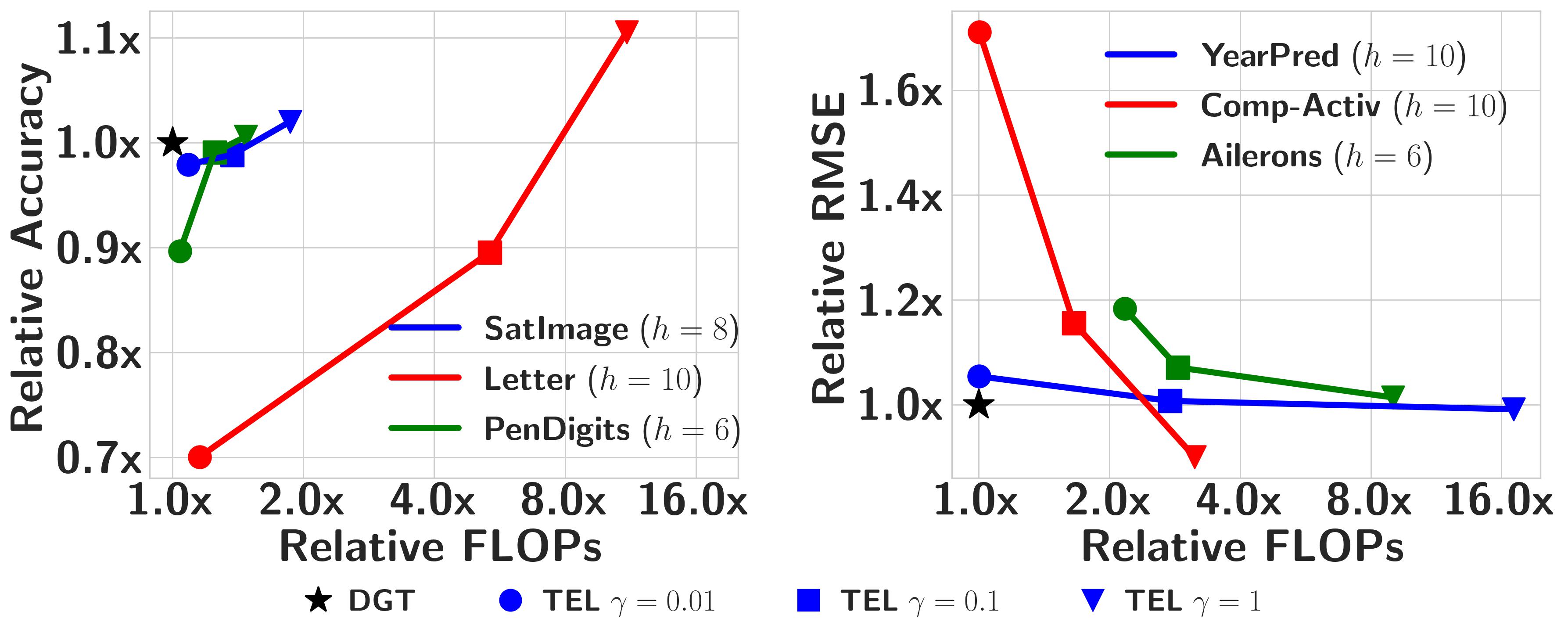
Figure 1: Performance vs. inference FLOPS (log scale) of the TEL method (for different $\gamma$ values that controls the number of leaves reached), relative to DGT, shown for the best performing heights for TEL on the respective datasets.

Dataset	DGT	TEL ($\gamma=1$)	TEL ($\gamma=0.1$)	TEL ($\gamma=0.01$)
PenDigits	96.36 $\pm$ 0.25	96.54 $\pm$ 0.46	95.10 $\pm$ 1.23	86.09 $\pm$ 2.53
SatImage	86.64 $\pm$ 0.95	87.64 $\pm$ 1.23	84.92 $\pm$ 0.94	84.12 $\pm$ 1.20
Letter	86.13 $\pm$ 0.72	95.21 $\pm$ 0.22	77.14 $\pm$ 0.98	60.35 $\pm$ 3.81
YearPred	9.05 $\pm$ 0.012	8.99 $\pm$ 0.067	9.14 $\pm$ 0.055	9.56 $\pm$ 0.081
Ailerons	1.72 $\pm$ 0.016	1.75 $\pm$ 0.062	1.85 $\pm$ 0.089	2.05 $\pm$ 0.013
Comp-Activ	2.91 $\pm$ 0.149	2.80 $\pm$ 0.205	3.60 $\pm$ 0.564	5.12 $\pm$ 0.863

Table 3: Performance comparison with soft trees on various classification and regression datasets. Results are computed over 10 runs with different random seeds. Numbers in the first 3 rows are mean test accuracy (%) $\pm$ std. deviation, and the last three rows are mean test RMSE $\pm$ std. deviation. For TEL we show performance with different settings of $\gamma$ leading to different degrees of softness.

5.2 Comparison to soft trees, ensembles and trees with linear leaves

Soft/Probabilistic trees.

DGT learns hard decision trees, with at most $d\cdot h$ FLOPS per inference, as against soft/probabilistic trees with exponential (in $h$) inference FLOPS (e.g., PAT method of Table 1 without annealing). In Tables  1 and  2, we note that state-of-the-art TEL method, with $\gamma=0.01$ (to ensure that at most 1 or 2 leaves are reached per example), performs significantly worse than DGT in almost all the datasets. We now look at the trade-off between computational cost and performance of TEL, that uses a carefully-designed activation function for predicates, instead of the standard sigmoid used in probabilistic trees. The hyper-parameter $\gamma$ in TEL controls the softness of the tree, affecting the number of leaves an example lands in, and in turn, the inference FLOPS. In Figure 1, we show the relative performance (i.e. ratio of accuracy or RMSE of TEL to that of DGT for a given height) vs relative FLOPS (i.e. ratio of mean inference FLOPS of TEL to that of DGT for a given height) of TEL, for different $\gamma$ values. First, note that, by definition, DGT is at (1,1) in the plots. When $\gamma=0.01$, TEL achieves about $d\cdot h$ inference FLOPS on average, similar to that of a hard decision tree (as in Table 1), but its performance is significantly worse than DGT on all the datasets. On the other hand, TEL frequently outperforms DGT at $\gamma=1$ (for instance, on SatImage, it improves accuracy by $2$%), but at a significant computational cost (as much as 17x FLOPS over DGT). We also present the performance comparison between DGT and TEL (at different $\gamma$ settings) in Table  3. Overall, DGT achieves competitive performance while keeping the inference cost minimal.

Tree ensembles.

To put the results shown so far in perspective, we compare DGT to widely-used ensemble methods for supervised learning. To this end, we extend DGT to learn forests (DGT-Forest) using the bagging technique, where we train a fixed number of DGT tree models independently on a bootstrap sample of the training data and aggregate the predictions of individual models (via voting or averaging) to generate a prediction for the forest. We compare DGT-Forest with AdaBoost and XGBoost in Table 4. First, as expected, we see that DGT-Forest outperforms DGT (in Table 1) on all datasets. Next, DGT-Forest using only 30 trees outperforms the two tree ensemble methods that use as many as 1000 trees, on 3 out of 5 datasets, and is competitive in the other 2. We also find that our results improve over other standard ensemble methods, on the same datasets and splits, published in Zharmagambetov and Carreira-Perpinan (2020).

Trees with linear leaves.

While DGT produces oblique trees whose leaves contain a constant model (a learnt constant value), we also compare it with trees containing a linear model in the leaves. In general, a tree with linear leaves is more expressive than a tree of the same height with constant leaves. In Table 5 we present a comparison with such trees learnt by TAO. As expected, we see that these trees usually outperform those learnt by DGT.

Dataset	DGT-Forest	XGBoost	AdaBoost
Ailerons	1.65 $\pm$ 0.00 (6)	1.72 $\pm$ 0.00 (7)	1.75 $\pm$ 0.00 (15)
Abalone	2.08 $\pm$ 0.00 (8)	2.20 $\pm$ 0.00 (10)	2.15 $\pm$ 0.00 (10)
Comp-Activ	2.63 $\pm$ 0.08 (8)	2.57 $\pm$ 0.00 (10)	2.56 $\pm$ 0.11 (10)
CtSlice	1.22 $\pm$ 0.07 (10)	1.18 $\pm$ 0.00 (10)	1.31 $\pm$ 0.01 (10)
YearPred	8.91 $\pm$ 0.00 (8)	9.01 $\pm$ 0.00 (10)	9.21 $\pm$ 0.03 (15)

Table 4: Supervised tree ensembles: mean test RMSE $\pm$ std. deviation (over 10 runs with different random seeds) for forest methods on regression datasets. DGT-Forest uses 30 trees while XGBoost and AdaBoost use about 1000 trees. Maximum height of the trees is given in parentheses.

Dataset	DGT (with constant leaves)	TAO (with linear leaves)
Ailerons	1.72 $\pm$ 0.016	1.74 $\pm$ 0.01
Abalone	2.15 $\pm$ 0.026	2.07 $\pm$ 0.01
Comp-Activ	2.91 $\pm$ 0.149	2.58 $\pm$ 0.02
CtSlice	2.30 $\pm$ 0.166	1.16 $\pm$ 0.02
YearPred	9.05 $\pm$ 0.012	9.08 $\pm$ 0.03

Table 5: Comparing DGT trees with constant leaves and TAO trees with linear model in the leaves. Scores are mean test RMSE $\pm$ std. deviation (over 10 runs for DGT and over 5 runs for TAO as reported in Zharmagambetov and Carreira-Perpinan (2020)).

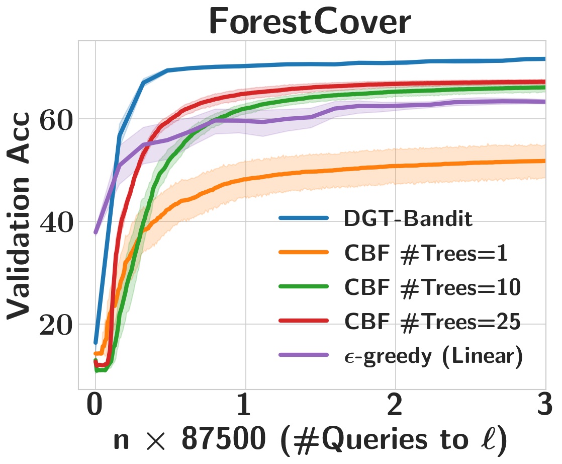
(a)

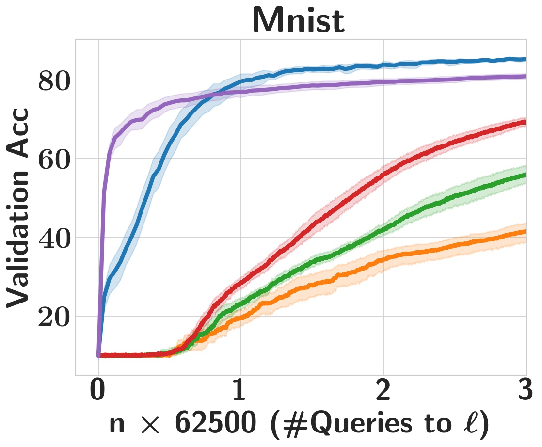
(b)

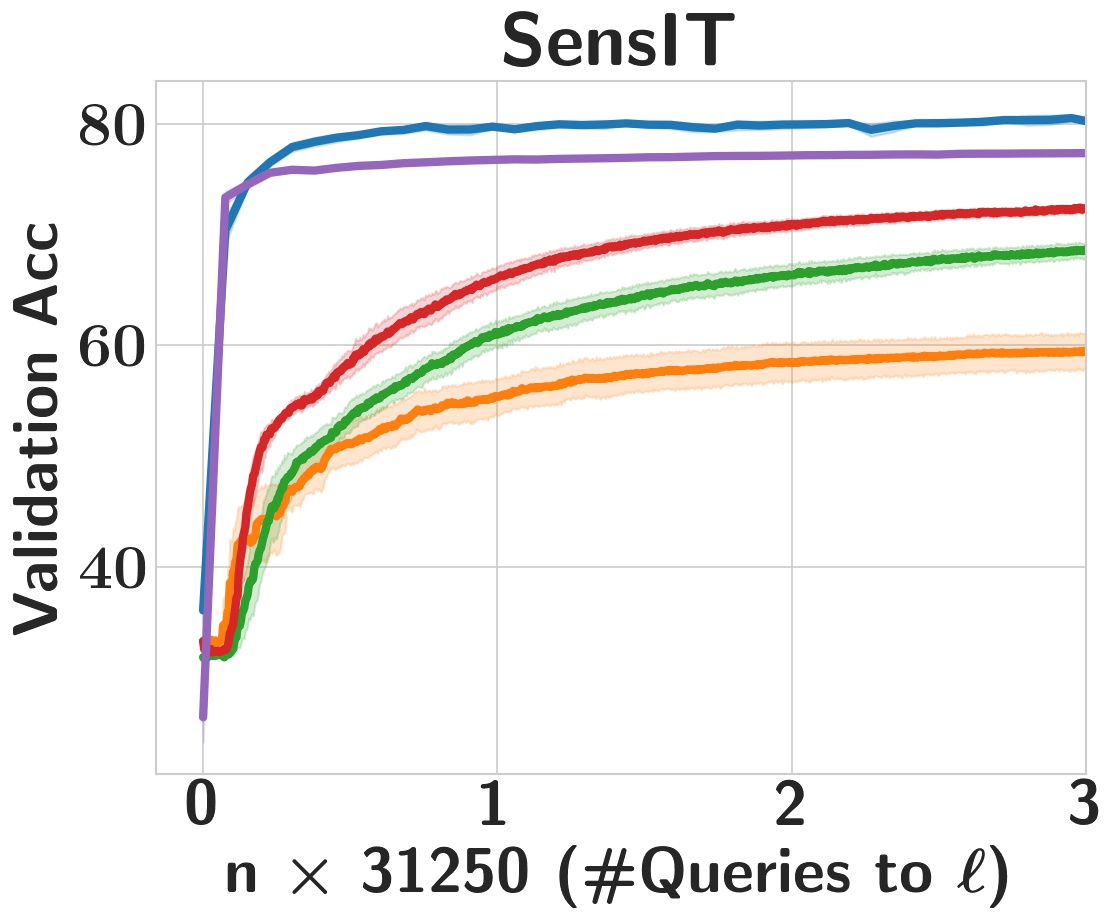
(c)

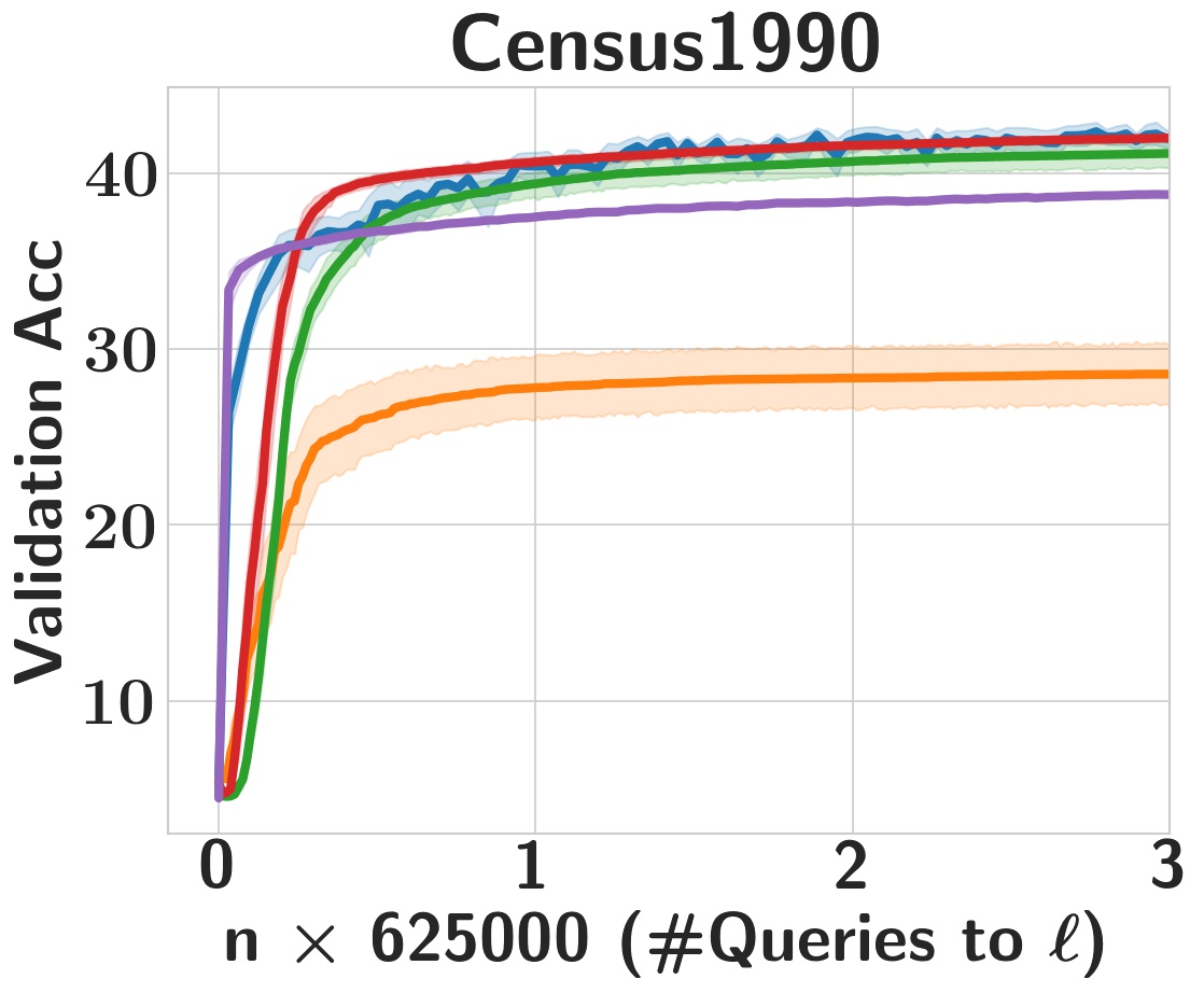
(d)

Figure 2: Bandit feedback setting (classification, one-point estimator in (8): #Queries to $\ell$ vs mean accuracy on held-out set for multi-class datasets over 10 runs, with $95\%$ confidence intervals. For DGT-Bandit, we use $h=6$ for all datasets except Census1990 where we use $h=8$.

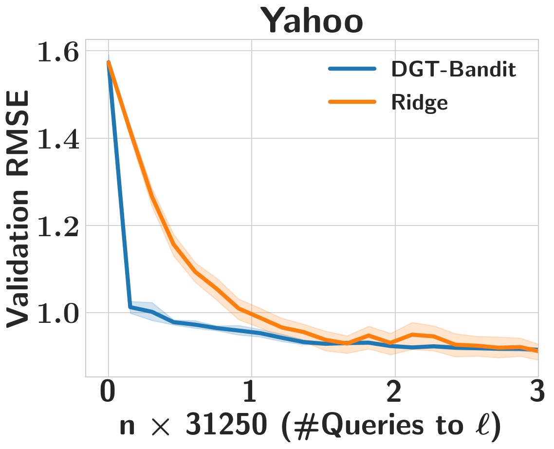
(a)

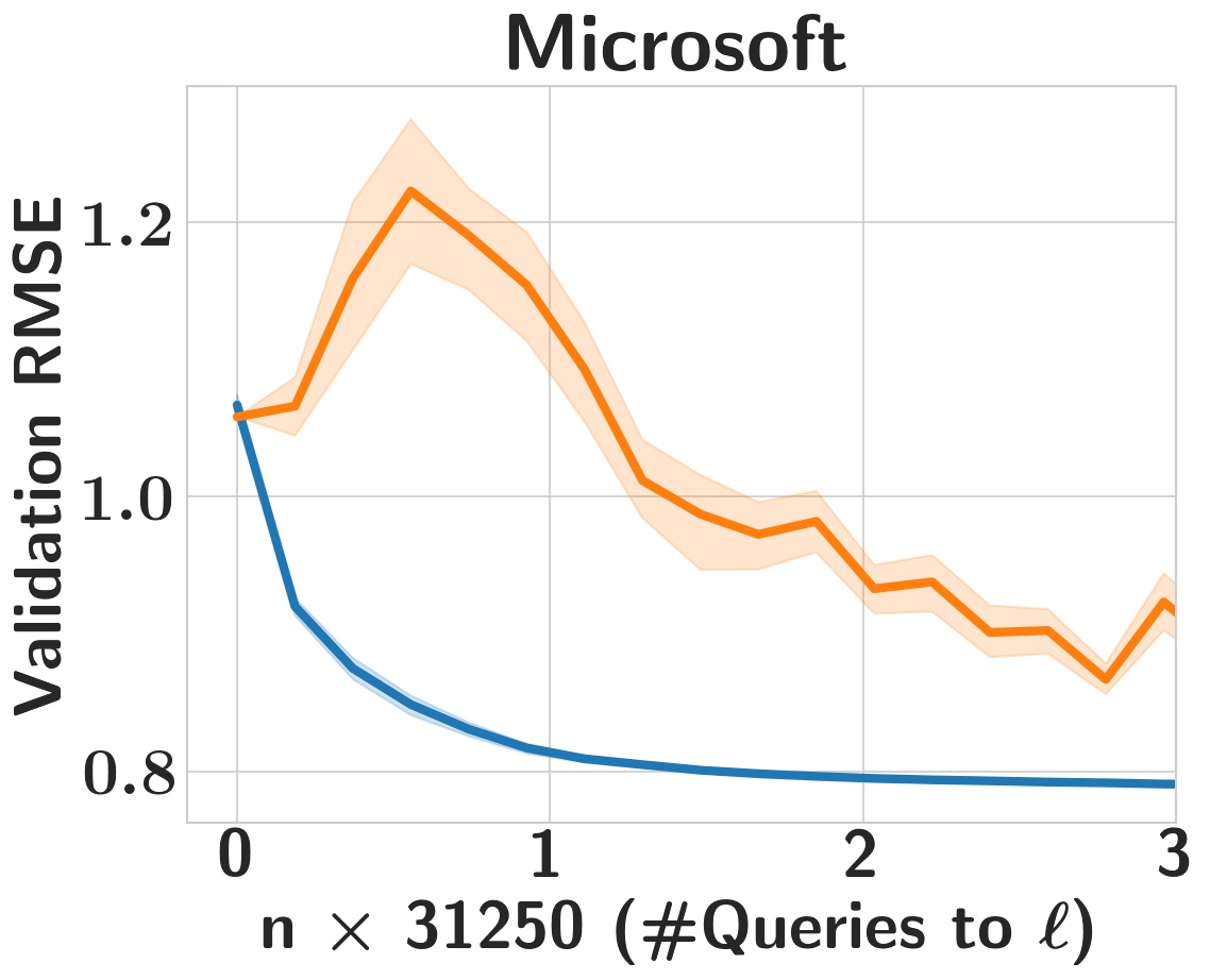
(b)

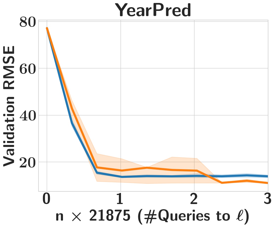
(c)

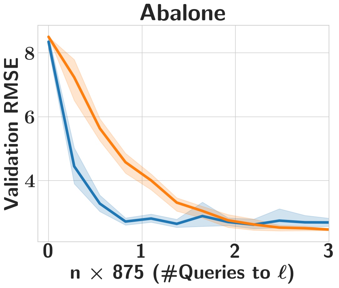
(d)

Figure 3: Bandit setting (regression, one-point estimator in (9)): #Queries to $\ell$ vs RMSE on held-out set for regression datasets, averaged over 10 runs and $95\%$ confidence intervals. Our method is run with default hyperparameters and $h=8$.

5.3 Bandit feedback setting

In the bandit setting, given a data point, we provide prediction using the tree function, and based on the loss for the prediction, we update the tree function. In particular, in this setting, neither the loss function nor the label information is available for the learner.

5.3.1 Classification

This is the standard contextual multi-armed bandit setting. Here, we compare with CBF (Féraud et al., 2016) and the $\epsilon$-greedy contextual bandits algorithm (Bietti et al., 2018) with linear policy class. Many SOTA tree-learning methods (Carreira-Perpinán and Tavallali, 2018; Zharmagambetov and Carreira-Perpinan, 2020; Bertsimas et al., 2019) do not apply to the bandit setting, as their optimization requires access to full loss function, so as to evaluate/update node parameters along different paths. For instance, standard extension of TAO would require evaluation of the loss function for a given point on $O(2^{h})$ predictions. Similarly, directly extending non-greedy method of Norouzi et al. (2015) would require $h+1$ queries to the loss $\ell$ on the same example per round, compared to DGT that can work with one loss function evaluation.

Results. We are interested in the sample complexity of the methods, i.e., how many queries to the loss $\ell$ is needed for the regret to become very small. In Figure 2, we show the convergence of accuracy against the #queries ($n$) to $\ell$ (0-1 loss) for DGT-Bandit (Algorithm 1), CBF (because their trees are axis-aligned, we use forests), and the $\epsilon$-greedy baseline, on the large multi-class classification datasets. Each point on the curve is the (mean) multi-class classification accuracy (and the shaded region corresponds to 95% confidence interval) computed on a fixed held-out set for the (tree) model obtained after $n$ rounds. It is clear that our method takes far fewer examples to converge to a fairly accurate solution in all the datasets shown. On ForestCover with 7 classes, after 10,000 queries (2% of train), our method achieves a test accuracy of 62.5% which is only 16% worse compared to the best solution achieved using full supervision. On Mnist, CBF (with 25 trees) takes nearly 400K queries ($\sim$6.7 passes over train) to reach an accuracy of $\sim$80%, which DGT-Bandit reaches within 76K queries ($\sim$1.25 passes).

5.3.2 Regression

We evaluate our method in this setting with two different losses (unknown to the learner): (a) squared loss $\ell_{\text{sq}}(\hat{y},y)=(\hat{y}-y)^{2}$, and (b) the Huber loss defined as:

$$\ell_{\xi}(\hat{y},y)=\begin{dcases*}\frac{1}{2}(\hat{y}-y)^{2},&\text{if } $|\hat{y}-y|\leq\xi$,\\ \xi|\hat{y}-y|-\frac{1}{2}\xi^{2},&\text{otherwise}.\end{dcases*}\vspace{-0.5cm}$$

We use ridge regression with bandit feedback as a baseline (which is as good as any tree method in the fully supervised setting, Table 1, on 4 out of 8 datasets) in this setting, for which gradient estimation is well known (using perturbation techniques described in Section 4).

Dataset	DGT-Bandit (Alg. 1)		Linear Regression
	Squared	Huber	Squared	Huber
Ailerons	1.71$\pm$0.016	1.72$\pm$0.016	1.78$\pm$0.003	1.87$\pm$0.001
Abalone	2.16$\pm$0.030	2.16$\pm$0.029	2.28$\pm$0.016	2.44$\pm$0.078
Comp-Activ	3.05$\pm$0.199	2.99$\pm$0.166	10.05$\pm$0.412	10.27$\pm$0.202
PdbBind	1.39$\pm$0.022	1.40$\pm$0.023	1.35$\pm$0.006	1.36$\pm$0.001
CtSlice	2.36$\pm$0.212	2.42$\pm$0.168	8.32$\pm$0.051	8.52$\pm$0.042
YearPred	9.05$\pm$0.013	9.06$\pm$0.008	9.54$\pm$0.002	9.68$\pm$0.003
Microsoft	0.772$\pm$0.000	0.773$\pm$0.001	0.781$\pm$0.000	0.782$\pm$0.000
Yahoo	0.796$\pm$0.001	0.797$\pm$0.002	0.810$\pm$0.001	0.815$\pm$0.000

Table 6: Bandit setting (regression): Mean test RMSE $\pm$ std. deviation (over 10 runs with different random seeds) using two-point estimator for $\ell^{\prime}$ in (10).

Results. We are interested in the sample complexity of the methods, i.e., how many queries to the loss $\ell$ is needed for the regret to become very small. In Figure 3, we show the convergence of RMSE against the # queries ($n$) to loss $\ell_{sq}$ for our method DGT-Bandit and the baseline (online) linear regression, both implemented using the one-point estimator for the derivative $\ell^{\prime}$ in (9). Each point on the curve is the RMSE computed on a fixed held-out set for the (tree) model obtained after $n$ rounds (in Algorithm 1). Our solution takes far fewer examples to converge to a fairly accurate solution in all the datasets shown. For instance, on the Yahoo dataset after 60,000 queries (13% of training data), our method achieves a test RMSE of $0.858$ which is only $7$% worse compared to the best solution achieved using full supervision (see Table 1).

In Table 6, we show a comparison of the methods implemented using the two-point estimator in (10), on all the regression datasets, for two loss functions. Here, we present the final test RMSE achieved by the methods after convergence. Not surprisingly, we find that our solution indeed does consistently better on most of the datasets. What is particularly striking is that, on many datasets, the test RMSE nearly matches the corresponding numbers (in Table 1) in the fully supervised setting where the exact gradient is known!

5.4 Ablative Analysis

Dataset	(a) Sum vs Prod. form $q_{l}$		(b) Overparameterization		(c) Quantization vs Anneal
	Prod, Eqn. (2)	Sum, Eqn. (4)	$L=1$	$L=3$	$\sigma_{s}$ + Anneal	$\operatorname{sign}$
Ailerons	2.02$\pm$0.028	1.72$\pm$0.016	1.90$\pm$0.026	1.72$\pm$0.016	1.73$\pm$0.021	1.72$\pm$0.016
Abalone	2.40$\pm$0.064	2.15$\pm$0.026	2.21$\pm$0.030	2.15$\pm$0.026	2.31$\pm$0.06	2.15$\pm$0.026
YearPred	9.72$\pm$0.063	9.05$\pm$0.012	9.18$\pm$0.017	9.05$\pm$0.012	9.18$\pm$0.04	9.05$\pm$0.012

Table 7: Ablation study of design choices in DGT(mean test RMSE $\pm$ std. deviation over 10 random seeds)

We empirically validate the key design choices of DGT motivated in Section 3. In all the cases, we vary only the aspect under study, fix all other implementation aspects to our proposed modeling choices, and report the performances of the best (cross-validated) models.
1. Sum vs Product forms for paths. In our formulation, we use the sum form of path function $q_{l}$ as given in (4). We also evaluate the multiplicative form in (2) (used in PAT). Table 7 (a) shows that the product form has consistently worse (e.g., over $17\%$ in Ailerons) RMSE across the datasets than the ones trained with the sum form in our method. This indicates that our hypothesis about gradient ill-conditioning for the product form holds true.
2. Effect of Overparameterization. Next, we study the benefit of learning a “deep embedding” for data points via multiple, linear, fully-connected layers as described in Section 3.2. It is not clear a priori why such “spurious” linear layers can help at all, as the hypothesis space remains the same. But, we find supportive evidence from Table 7 (b) that adding just 2 layers helps improve the performance in many datasets. On YearPred, overparameterization makes the difference between SOTA methods and ours. Recent findings (Arora et al., 2018) suggest that linear overparameterization helps optimization via acceleration. We find that a modest value of $L=3$ works across datasets. We defer a thorough study of this aspect and its implications to future work.
3. Quantization vs Annealing. Finally, we study the effectiveness of the quantized gradient updates, i.e., using the $\operatorname{sign}$ function in the forward pass, and the straight-through estimator to compute its gradient in the backward pass. We compare against the annealing technique for scaled sigmoid function $\sigma_{s}(a)=\frac{1}{1+\exp(-s\cdot a)}$, i.e., slowly increasing the value of $s$ during training. Table 7 (c) suggests that the quantized updates are crucial for DGT; on Abalone, annealing performs worse than all the methods in Table 1, except PAT which it improves over because of overparameterization and the use of sum form.

6 Conclusions

We proposed an end-to-end gradient-based method for learning hard decision trees that admits dense updates to all tree parameters. DGT enables learning trees in several practical scenarios, such as supervised learning and online learning with limited feedback. Our comprehensive experiments in the supervised setting demonstrated that DGT achieves nearly SOTA performance on several datasets. On the other hand, in the bandit setting, where most existing techniques do not even apply, DGT yields accurate solutions with low sample complexity, and in many cases, matches the performance of our offline-trained models. In our experiments, default hyperparameters worked well (see Appendix C.3), but it is unclear how to set them in real-world online deployments where dataset characteristics might be significantly different. We plan to explore relevant approaches from parameter-free online learning literature (Chap. 9, Orabona (2019)). Understanding linear overparameterization, extending quantization techniques to learning trees with higher out-degree, and deploying  DGT in ML-driven systems that need accurate, low cost models, are potential directions at this point.

Appendix A Tree Learning Algorithm Variants

Our method DGT for learning decision trees in the standard supervised learning setting is given in Algorithm 3. Note that here we know the loss function $\ell$ exactly, so computing the gradient is straight-forward (in Step 9). Also, the dot product in Step 9 (as well as in Steps 11 and 12 of Algorithm 1) is appropriately defined when $K>1$, as it involves a vector and a tensor. The back propagation procedure, which is used both in DGT and in DGT-Bandit (Algorithm 1), is given in Algorithm 2 ($K=1$ case, for clarity).

1:Input: training data $(\mathbf{x}_{i},y_{i})_{i=1}^{n}$, height $h$, max epochs $\tau_{\max}$, learning rate $\eta$, loss $\ell$, regularization ($\lambda,\Phi_{\text{reg}}$), overparameterization $L$, hidden dim $d_{i}$, $i\in[L]$

2:Output: Tree model: $\mathbf{W},$ and $\boldsymbol{\Theta}\in\mathbb{R}^{2^{h}\times K}$

3:

4:Init: $\mathbf{W}_{0}^{(1)}\in\mathbb{R}^{d_{1}\times d},\mathbf{W}_{0}^{(2)}\in\mathbb{R}^{d_{2}\times d_{1}},\dots,\mathbf{W}_{0}^{(L)}\in\mathbb{R}^{(2^{h}-1)\times d_{L-1}},\boldsymbol{\Theta}_{0}$ randomly.

5:$\mathbf{x}_{i}=[\mathbf{x}_{i};\ 1]$ for $i=1,2,\dots,n$ // incorporate bias

6:for epoch $1\leq\tau\leq\tau_{\max}$ do

7:     $(\mathbf{W},\boldsymbol{\Theta})=(\mathbf{W}_{\tau-1},\boldsymbol{\Theta}_{\tau-1})$

8:     for each mini-batch $B$ do // perform SGD on mini-batches

9:         $\boldsymbol{\theta}_{l}=f(\mathbf{x}_{i};\mathbf{W},\boldsymbol{\Theta})$, $i\in B$ (via (2), and hard $\sigma$ in (3)) // Compute the tree model prediction

10:         $\{\nabla_{\mathbf{W}^{(m)}}\ell,\nabla_{\boldsymbol{\Theta}}\ell\}\leftarrow\frac{1}{|B|}\displaystyle\sum_{i\in B}\nabla_{\boldsymbol{\theta}_{l}}\ell(y_{i},\boldsymbol{\theta}_{l})\ \cdot$ BackProp$(\mathbf{x}_{i};\mathbf{W},\boldsymbol{\Theta})$ // Algorithm 2

11:         $\mathbf{W}^{(m)}\leftarrow\mathbf{W}^{(m)}-\eta\nabla_{\mathbf{W}^{(m)}}\ell-\eta\lambda\nabla_{\mathbf{W}^{(m)}}\Phi_{\text{reg}}(\mathbf{W},\boldsymbol{\Theta})$,  for $m=1,2,\dots,L$.

12:         $\boldsymbol{\Theta}\leftarrow\boldsymbol{\Theta}-\eta\nabla_{\boldsymbol{\Theta}}\ell-\eta\lambda\nabla_{\boldsymbol{\Theta}}\Phi_{\text{reg}}(\mathbf{W},\boldsymbol{\Theta})$      

13:     $(\mathbf{W}_{\tau},\boldsymbol{\Theta}_{\tau})=(\mathbf{W},\boldsymbol{\Theta})$

14:return $\mathbf{W}_{\tau_{\max}},\boldsymbol{\Theta}_{\tau_{\max}}$

Algorithm 3 DGT: Learning decision trees in the supervised learning (batch) setting

Appendix B Datasets Description

Whenever possible we use the train-test split provided with the dataset. In cases where a separate validation split is not provided, we split training dataset in $0.8:0.2$ proportion to create a validation. When no splits are provided, we create five random splits of the dataset and report the mean test scores across those splits, following Zharmagambetov and Carreira-Perpinan [2020]. Unless otherwise specified, we normalize the input features to have mean $0$ and standard deviation $1$ for all datasets. Additionally, for regression datasets, we min-max normalize the target to $[0,1]$.

B.1 Regression datasets

We used eight scalar regression datasets comprised of the union of datasets used in  Popov et al. [2020], Lee and Jaakkola [2020], Zharmagambetov and Carreira-Perpinan [2020]. Table 9 summarizes the dataset details.

• Ailerons : Given attributes describing the status of the aircraft, predict the command given to its ailerons.

• Abalone : Given attributes describing physical measurements, predict the age of an abalone. We encode the categorical (“sex") attribute as one-hot.

• Comp-Activ : Given different system measurements, predict the portion of time that CPUs run in user mode. Copyright notice can be found here: http://www.cs.toronto.edu/ delve/copyright.html.

• CtSlice : Given attributes as histogram features (in polar space) of the Computer Tomography (CT) slice, predict the relative location of the image on the axial axis (in the range [$0$ $180$]).

• PdbBind : Given standard “grid features" (fingerprints of pairs between ligand and protein; see Wu et al. [2018]), predict binding affinities. MIT License (https://github.com/deepchem/deepchem/blob/master/LICENSE).

• YearPred : Given several song statistics/metadata (timbre average, timbre covariance, etc.), predict the age of the song. This is a subset of the UCI Million Songs dataset.

• Microsoft : Given 136-dimensional feature vectors extracted from query-url pairs, predict the relevance judgment labels which take values from 0 (irrelevant) to 4 (perfectly relevant).

• Yahoo : Given 699-dimensional feature vectors from query-url pairs, predict relevance values from 0 to 4.

B.2 Classification datasets

We use eight multi-class classification datasets from Carreira-Perpinán and Tavallali [2018], two multi-class classification datasets from  Féraud et al. [2016] and two binary classification datasets from from Lee and Jaakkola [2020]. Table 8 summarizes the dataset details.

• Protein : Given features extracted from amino acid sequences, predict secondary structure for a protein sequence.

• PenDigits : Given integer attributes of pen-based handwritten digits, predict the digit.

• Segment : Given 19 attributes for each 3x3 pixel grid of instances drawn randomly from a database of 7 outdoor colour images, predict segmentation of the central pixel.

• SatImage : Given multi-spectral values of pixels in 3x3 neighbourhoods in a satellite image, predict the central pixel in each neighbourhood.

• SensIT : Given 100 relevant sensor features, classify the vehicles.

• Connect4 : Given legal positions in a game of connect-4, predict the game theoretical outcome for the first player.

• Mnist : Given 784 pixels in handwritten digit images, predict the actual digit.

• Letter : Given 16 attributes obtained from stimulus observed from handwritten letters, classify the actual letters.

• ForestCover : Given 54 cartographic variables of wilderness areas, classify forest cover type.

• Census1990 : Given 68 attributes obtained from US 1990 census, classify the Yearsch column.

• HIV : Given standard Morgan fingerprints (2,048 binary indicators of chemical substructures), predict HIV replication. MIT License (https://github.com/deepchem/deepchem/blob/master/LICENSE).

• Bace : Given standard Morgan fingerprints (2,048 binary indicators of chemical substructures), predict binding results for a set of inhibitors. MIT License (https://github.com/deepchem/deepchem/blob/master/LICENSE).

Table 8: Classification datasets description

dataset	# features	# classes	train size	splits (tr:val:test)	# shuffles	source
Connect4	126	3	43,236	$0.64:0.16:0.2$	1	LIBSVM
Mnist	780	10	48,000	Default	1	LIBSVM2
Protein	357	3	14,895	Default3	1	LIBSVM2
SensIT	100	3	63,058	Default5	1	LIBSVM2
Letter	16	26	10,500	Defaul3	1	LIBSVM2
PenDigits	16	10	5,995	Default3	1	LIBSVM2
SatImage	36	6	3,104	Default3	1	LIBSVM2
Segment	19	7	1,478	$0.64:0.16:0.2$	1	LIBSVM2
ForestCover	54	7	371,846	$0.64:0.16:0.2$	1	UCI8
Census1990	68	18	1,573,301	$0.64:0.16:0.2$	1	UCI8
Bace	2,048	2	1,210	Default3	1	MoleculeNet
HIV	2,048	2	32,901	Default3	1	MoleculeNet4

Table 9: Regression datasets description

dataset	# features	train size	splits (tr:val:test)	# shuffles	source
Ailerons	40	5,723	Default3	1	LIACC
Abalone	10	2,004	$0.5:0.1:0.4$	5	UCI8,
Comp-Activ	21	3,932	$0.5:0.1:0.4$	5	Delve,6
CtSlice	384	34,240	$0.5:0.1:0.4$	5	UCI8,6
PdbBind	2,052	9,013	Default3	1	MoleculeNet4
YearPred	90	370,972	Default3	1	UCI
Microsoft	136	578,729	Default3	1	MSLR-WEB10K
Yahoo	699	473,134	Default3	1	Yahoo Music Ratings

Appendix C Evaluation Details and Additional Results

All scores are computed over 10 runs, differing in the random initialization done, except for TAO on regression datasets which uses 5 runs. In all the experiments, for a fixed tree height and a dataset, our DGT implementation takes $\leq$ 20 minutes for training (and $\leq$ 1 hour including hyper-parameter search over four GPUs.)

Dataset	DGT (Alg. 3)	TAO	LCN	TEL	CART
Protein	67.80$\pm$0.40 (4)	68.41$\pm$0.27	67.52$\pm$0.80	67.63$\pm$0.61	57.53$\pm$0.00
PenDigits	96.36$\pm$0.25 (8)	96.08$\pm$0.34	93.26$\pm$0.84	94.67$\pm$1.92	89.94$\pm$0.34
Segment	95.86$\pm$1.16 (8)	95.01$\pm$0.86	92.79$\pm$1.35	92.10$\pm$2.02	94.23$\pm$0.86
SatImage	86.64$\pm$0.95 (6)	87.41$\pm$0.33	84.22$\pm$1.13	84.65$\pm$1.18	84.18$\pm$0.30
SensIT	83.67$\pm$0.23 (10)	82.52$\pm$0.15	82.02$\pm$0.77	83.60$\pm$0.16	78.31$\pm$0.00
Connect4	79.52$\pm$0.24 (8)	81.21$\pm$0.25	79.71$\pm$1.16	80.68$\pm$0.44	74.03$\pm$0.60
Mnist	94.00$\pm$0.36 (8)	95.05$\pm$0.16	88.90$\pm$0.63	90.93$\pm$1.37	85.59$\pm$0.06
Letter	86.13$\pm$0.72 (10)	87.41$\pm$0.41	66.34$\pm$0.88	60.35$\pm$3.81	70.13$\pm$0.08
ForestCover	79.25$\pm$0.50 (10)	83.27$\pm$0.32	67.13$\pm$3.00	73.47$\pm$0.83	77.85$\pm$0.00
Census1990	46.21$\pm$0.17 (8)	47.22$\pm$0.10	44.68$\pm$0.45	37.95$\pm$1.95	46.40$\pm$0.00
HIV	0.712$\pm$0.020	0.627$\pm$0.000	0.738$\pm$0.014	-	0.562$\pm$0.000
Bace	0.767$\pm$0.045	0.734$\pm$0.000	0.791$\pm$0.019	0.810$\pm$0.028	0.697$\pm$0.000

Table 10: Fully supervised setting: Comparison of tree learning methods on various classification datasets. Results are computed over 10 runs with different random seeds. Numbers in the first 10 rows are mean test accuracy (%) $\pm$ std. deviation, and the last 2 rows are mean test AUC $\pm$ std. deviation. For TEL, we set $\gamma=0.01$.

C.1 Height-wise results for the fully supervised setting

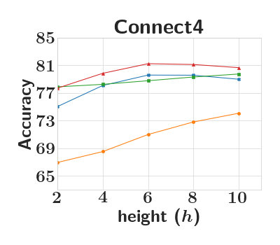
(a)

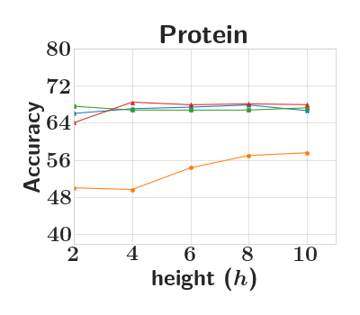
(b)

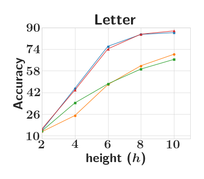
(c)

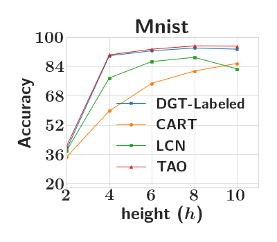
(d)

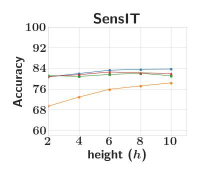
(e)

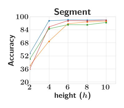
(f)

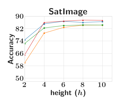
(g)

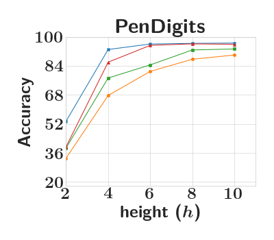
(h)

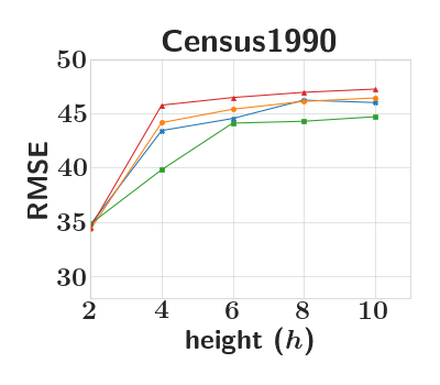
(i)

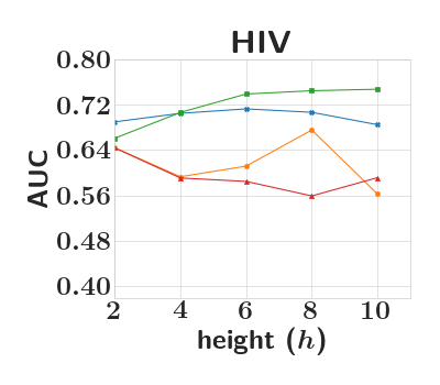
(j)

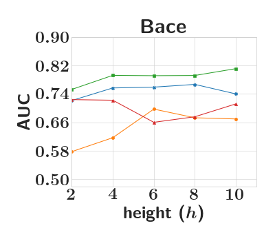
(k)

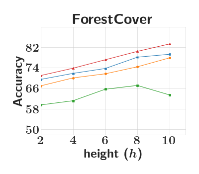
(l)

Figure 5: Mean (%) Test Accuracy or Test AUC of competing methods (over 10 random seeds) vs tree height for classification datasets.

Heightwise results for our method DGT and compared methods on various regression and classification datasets can be found in Fig. 4 and Fig. 5 respectively. As mentioned in Section 5.1, we find that the numbers obtained from our implementation of TAO [Zharmagambetov and Carreira-Perpinan, 2020] differ from their reported numbers on some datasets; so we quote numbers directly from their paper in Table 1, where available. Keeping up with that, in Figure 4, we present height-wise results for the TAO method only on the 3 datasets that they do not report results on. We do not present heightwise results for TEL as we find that the method is generally poor across heights when we restrict $\gamma$ to be small ($\sim 0.01$).

C.2 Sparsity of learned tree models

Though we learn complete binary trees, we find that the added regularization renders a lot of the nodes in the learned trees expendable, and therefore can be pruned. For instance, out of 63 internal nodes in a height 6 Ailerons tree (best model), only 47 nodes receive at least one training point. Similarly, for a height 8 Yahoo tree (best model), only 109 nodes out of total 255 nodes receive at least one training point. These examples indicate that the trees learned by our method can be compressed substantially.

Table 11: Hyperparameter selection for our method: we use default values for many, and cross-validated over the given sets for the last 3.

hyperparameter	Default Value or Range
Optimizer	RMSprop
Learning Rate	$1e\text{-}2$
Learning Rate Scheduler	CosineLR Scheduler ($3$ restarts)
Gradient Clipping	$1e\text{-}2$
Mini-batch size	$128$
Epochs	$30$-$400$ (depending on dataset size)
Overparameterization ($L$)	$\{1,3\}$ (hidden dimensions in Table 12)
Regularization ($\lambda_{1}$ or $\lambda_{2}$)	$\{5e\text{-}5,1e\text{-}5,5e\text{-}6,1e\text{-}6,0\}$ if $L>1$ else $0$
Momentum	$\{0,0.3\}$ if regression else $\{0,0.3,0.8\}$

C.3 Implementation details

C.3.1 Offline/batch setting

DGT

We implement the quantization and $\arg\max$ operations in PyTorch as autograd functions. Below, we give details of hyperparameter choices for any given height ($h\in\{2,4,6,8,10\}$).
We train using RMSProp optimizer with learning-rate $1e\text{-}2$ and cosine scheduler with $3$ restarts; gradient clipping $1e\text{-}2$; momentum of optimizer $\in\{0,0.3\}$ for regression and $\{0,0.3,0.8\}$ for classification; regularization $\lambda_{1},\lambda_{2}\in\{5e\text{-}5,1e\text{-}5,5e\text{-}6,1e\text{-}6,0\}$; and overparameterization $L\in\{1,3\}$ with hidden space dimensions given in Table 12. We use a mini-batch size of $128$ and train our model for $30$-$400$ epochs based on the size of dataset. Table 11 summarizes the choices for all the hyperparameters. Note that we use default values for most of the hyperparameters, and cross-validate only a few.

Table 12: Hidden dimensions for overparameterization ($L=3$): we use a fixed set of $d_{i}$’s for a given height $h$; note $d_{3}=2^{h}-1$.

Height	Hidden dimensions
2	$[240,\ 240,\ 3]$
4	$[600,\ 600,\ 15]$
6	$[1008,\ 1008,\ 63]$
8	$[1530,\ 1530,\ 255]$
10	$[2046,\ 2046,\ 1023]$

DGT-Forest

We extend DGT to learn forests (DGT-Forest, presented in Section 5.2) using the bagging technique, where we train a fixed number of DGT tree models independently on a bootstrap sample of the training data and aggregate the predictions of individual models (via averaging for regression and voting for classification) to generate a prediction for the forest. The number of tree models trained is set to $30$. The sample of training data used to train each tree model is generated by randomly sampling with replacement from the original training set. The sample size for each tree relative to the full training set is chosen from $\{0.7,0.85,0.9,1\}$. Hyperparameters for the individual tree models are chosen as given previously for DGT, with the following exceptions: momentum of optimizer $\in\{0,0.2,0.3,0.4,0.6\}$ and regularization is used even when $L=1$.

TAO

We implemented TAO in Python since the authors have not made the code available yet [Zharmagambetov, April 2021]. For optimization over a node, we use scikit-learn’s LogisticRegression with the liblinear solver . For the classification datasets, we initialize the tree with CART (trained using scikit-learn) as mentioned in Carreira-Perpinán and Tavallali [2018], train for $40$ iterations, where for the LogisticRegression learner, we set maxiter$=20$, tol$=5e\text{-}2$ and cross-validate $\lambda_{1}\in\{1e\text{-}4,1e\text{-}3,1e\text{-}2,1e\text{-}1,1,10,30\}$. The results we obtain are close to/marginally better than that inferred from the figures in the supplementary material of Carreira-Perpinán and Tavallali [2018].

For the regression datasets we initialize the predicates in the tree randomly as mentioned in Zharmagambetov and Carreira-Perpinan [2020]. For PdbBind, we initialize the leaves randomly in $[0,1)$, train for $40$ iterations, set maxiter $=20$, tol $=5e\text{-}2$ and cross-validate $\lambda_{1}\in\{1e\text{-}3,1e\text{-}2,1e\text{-}1,1\}$. For the large datasets, Microsoft and Yahoo, we initialize all leaves to $1$, train for $20$ iterations with maxiter $=20$, tol $=1e\text{-}2$ and cross-validate $\lambda_{1}\in\{1e\text{-}3,1e\text{-}2,1e\text{-}1\}$. In all cases, post-training, as done by the authors, we prune the tree to remove nodes which don’t receive any training data points. For the other regression datasets, despite our efforts, we weren’t able to reproduce the reported numbers, so we have not provided height-wise results for those (in Figure 4).

LCN

We use the publicly available implementation of LCN provided by the authors. On all classification and regression datasets we run the algorithm for $100$ epochs, using a batch size of $128$ (except for the large datasets YearPred, Microsoft and Yahoo where we use $512$) and cross validate on: two optimizers - Adam (AMSGrad variant) and SGD (Nesterov momentum factor $0.9$ with learning rate halving every $20$ epochs); learning rate $\in\{1e\text{-}5,1e\text{-}4,3e\text{-}4,1e\text{-}3,3e\text{-}3,1e\text{-}2,3e\text{-}2,1e\text{-}1,3e\text{-}1,1\}$; dropout probability $\in\{0,0.25,0.5,0.75\}$; number of hidden layers in $g_{\phi}$ $\in\{0,1,2,3,4,5\}$ and between the model at the end of training vs. the best performing early-stopped model. On HIVand PdbBind we were able to improve on their reported scores.

TEL

We use the publicly available implementation [TEL, ]. We use the Adam optimizer with mini-batch size of 128 and cross-validate learning rate $\in\{1e\text{-}5,1e\text{-}4,1e\text{-}3,1e\text{-}2,1e\text{-}1\}$, $\lambda_{2}\in\{0,1e\text{-}8,1e\text{-}6,1e\text{-}4,1e\text{-}3,1e\text{-}2,1e\text{-}1,1,10,100\}$. The choice of $\gamma\in\{1e\text{-}4,1e\text{-}3,1e\text{-}2,1e\text{-}1,1\}$ is explicitly specified in Section 5 when we present the results for this method. To compute the (mean relative) FLOPS, we measure the number of nodes encountered by their model during inference for each test example, and compute the average.

PAT and ablations

For the probabilistic annealed tree model (presented in Table 1 as well as in Table 7(c)), we use a sigmoid activation on the predicates and softmax activation after the AND layer. We tune the annealing of the softmax activation function with both linear and logarithmic schedules over the ranges [[1,100],[1,1000],[1,10000],[10,100],[10,1000],[10,10000]]. Additionally we tune momentum of optimizer. We follow similar annealing schedules in quantization ablation as well but use additive AND layer and overparameterization instead.

CART

We use the CART implementation that is part of the scikit-learn Python library. We cross-validated min_samples_leaf over values sampled between $2$ and $150$.

Ridge

We use the Ridge implementation that is part of the scikit-learn Python library. We cross-validated the regularization parameter over 16 values between $1e\text{-}6$ and $5e\text{-}1$.

C.3.2 Online/bandit setting

In the online/bandit classification setting, we do not perform any dataset dependent hyperparameter tuning for any of the methods. Instead we try to pick hyperparameter configurations that work consistently well across the datasets.

DGT-Bandit

For the classification setting we remove gradient clipping and learning rate scheduler. We further restrict to $L=1$, $\lambda_{1}=0$, $\lambda_{2}=0$, momentum $=0$ (and mini-batch size $=1$, by virtue of the online setting and accumulate gradient over four steps). We use the learning rate and $\delta$ parameter which work consistently across all datasets. For the classification case we set $\delta$ (exploration probability in Eqn. (7)) to $0.3$ and $\delta$ parameter in Eqn. (10) and Eqn. (9) to $0.5$. Learning rate $1e\text{-}3$ is used. For the regression setting we only tune the learning rate $\in$ $\{1e\text{-}2$,$1e\text{-}3\}$, $\delta\ \in$ $\{1$,$0.5$,$0.1$,$0.05$,$0.01$,$0.001\}$ and momentum of optimizer.

Linear Regression

We implemented linear regression for the bandit feedback setup in PyTorch. We use RMSprop optimizer and we tune the learning rate $\in\{1e\text{-}2,1e\text{-}3\}$, momentum $\in\{0,0.4,0.8\}$, regularization $\in\{1,0.5,0.1,0.05,0.01\}$. We use number of epochs similar to our method. To compute the gradient estimate, we vary $\delta~{}(\text{in Eqn.}~{}\eqref{eqn:onepoint})\in\{1,0.5,0.1,0.05,0.01,0.001\}$.

$\epsilon$-Greedy (Linear)

For linear contextual-bandit algorithm with $\epsilon$-greedy exploration (Equation 6 and Algorithm 2 in Bietti et al. [2018]), we use VowpalWabbit [VW, ] with the --cb_explore and --epsilon flags. We tune learning rate $\eta\in\{0.001,0.01,0.1,1\}$ and the probability of exploration $\epsilon\in\{0.01,0.1,0.3,0.5\}$. We use $\eta=0.01,\epsilon=0.5$ which work well across all the datasets.

CBF

We use the official implementation provided by the authors [CBF, ] and use the default hyperparameter configuration for all datasets. Since their method works with only binary features, we convert the categorical features into binary feature vectors and discretize the continuous features into 5 bins, following their work [Féraud et al., 2016].

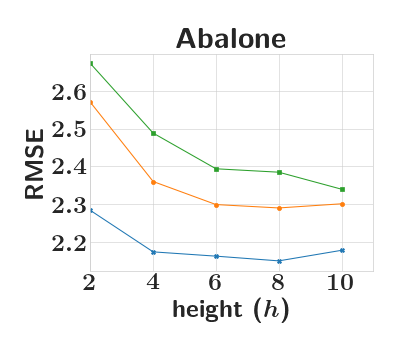
(a)

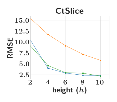
(b)

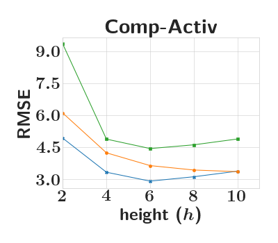
(c)

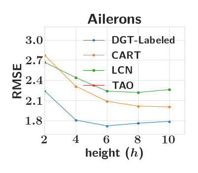
(d)

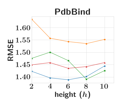
(e)

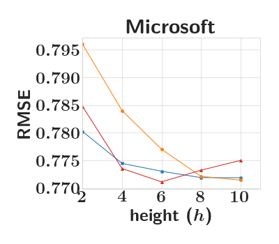
(f)

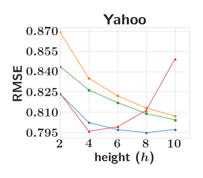
(g)

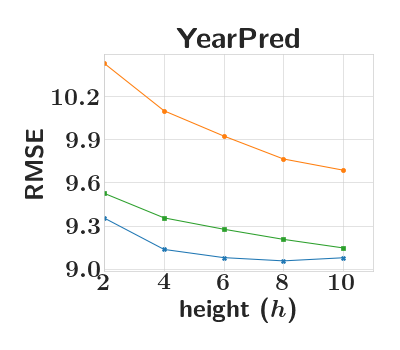
(h)

Figure 4: Mean Test RMSE (over 10 random seeds) of competing methods vs tree height for regression datasets. We do not show the performance of TAO method on some datasets (see Sections 5.1 and C.1). LCN did not converge on Microsoft (see Section 5.1).

References

- [1] Contextual bandit forests (CBF). https://www.researchgate.net/publication/294085581_Random_Forest_for_the_Contextual_Bandit_Problem.
- [2] Locally-constant networks (LCN). https://github.com/guanghelee/iclr20-lcn.
- [3] Tree Ensemble Layer. https://github.com/google-research/google-research/tree/master/tf_trees.
- [4] Vowpal Wabbit. https://vowpalwabbit.org.
- Agarwal et al. [2010] Alekh Agarwal, Ofer Dekel, and Lin Xiao. Optimal algorithms for online convex optimization with multi-point bandit feedback. In COLT, pages 28–40. Citeseer, 2010.
- Agarwal et al. [2014] Alekh Agarwal, Daniel Hsu, Satyen Kale, John Langford, Lihong Li, and Robert Schapire. Taming the monster: A fast and simple algorithm for contextual bandits. In International Conference on Machine Learning, pages 1638–1646, 2014.
- Allen-Zhu et al. [2019] Z Allen-Zhu, Y Li, and Y Liang. Learning and Generalization in Overparameterized Neural Networks, Going Beyond Two Layers. In Advances in Neural Information Processing Systems, 2019.
- Allesiardo et al. [2014] Robin Allesiardo, Raphaël Féraud, and Djallel Bouneffouf. A neural networks committee for the contextual bandit problem. In The 21st International Conference on Neural Information Processing, pages 374–381, 2014.
- Arora et al. [2018] Sanjeev Arora, Nadav Cohen, and Elad Hazan. On the optimization of deep networks: Implicit acceleration by overparameterization. In International Conference on Machine Learning, pages 244–253. PMLR, 2018.
- Arora et al. [2019] Sanjeev Arora, Simon Du, Wei Hu, Zhiyuan Li, and Ruosong Wang. Fine-grained analysis of optimization and generalization for overparameterized two-layer neural networks. In International Conference on Machine Learning, pages 322–332. PMLR, 2019.
- Balestriero [2017] Randall Balestriero. Neural decision trees. arXiv preprint arXiv:1702.07360, 2017.
- Bengio et al. [2013] Yoshua Bengio, Nicholas Léonard, and Aaron Courville. Estimating or propagating gradients through stochastic neurons for conditional computation. arXiv preprint arXiv:1308.3432, 2013.
- Bertsimas and Dunn [2017] Dimitris Bertsimas and Jack Dunn. Optimal classification trees. Machine Learning, 106(7):1039–1082, 2017.
- Bertsimas et al. [2019] Dimitris Bertsimas, Jack Dunn, and Nishanth Mundru. Optimal prescriptive trees. INFORMS Journal on Optimization, 1(2):164–183, 2019.
- Biau et al. [2019] Gérard Biau, Erwan Scornet, and Johannes Welbl. Neural random forests. Sankhya A, 81(2):347–386, 2019.
- Bietti et al. [2018] Alberto Bietti, Alekh Agarwal, and John Langford. A contextual bandit bake-off. arXiv preprint arXiv:1802.04064, 2018.
- Breiman et al. [1984] Leo Breiman, Jerome Friedman, Charles J Stone, and Richard A Olshen. Classification and regression trees. CRC press, 1984.
- Carreira-Perpinán and Tavallali [2018] Miguel A Carreira-Perpinán and Pooya Tavallali. Alternating optimization of decision trees, with application to learning sparse oblique trees. In Advances in Neural Information Processing Systems, pages 1211–1221, 2018.
- Courbariaux et al. [2016] Matthieu Courbariaux, Itay Hubara, Daniel Soudry, Ran El-Yaniv, and Yoshua Bengio. Binarized neural networks: Training deep neural networks with weights and activations constrained to +1 or -1. arXiv preprint arXiv:1602.02830, 2016.
- Dani et al. [2008] Varsha Dani, Thomas P Hayes, and Sham M Kakade. Stochastic linear optimization under bandit feedback. 21st Annual Conference on Learning Theory, 2008.
- Das et al. [2019] Ariyam Das, Jin Wang, Sahil M Gandhi, Jae Lee, Wei Wang, and Carlo Zaniolo. Learn smart with less: Building better online decision trees with fewer training examples. In IJCAI, pages 2209–2215, 2019.
- Dietterich et al. [1997] Thomas G Dietterich, Richard H Lathrop, and Tomás Lozano-Pérez. Solving the multiple instance problem with axis-parallel rectangles. Artificial intelligence, 89(1-2):31–71, 1997.
- Domingos and Hulten [2000] Pedro Domingos and Geoff Hulten. Mining high-speed data streams. In Proceedings of the sixth ACM SIGKDD International Conference on Knowledge Discovery and Data Mining, pages 71–80, 2000.
- Dudík et al. [2011] Miroslav Dudík, John Langford, and Lihong Li. Doubly robust policy evaluation and learning. In Proceedings of the 28th International Conference on International Conference on Machine Learning, ICML’11, page 1097–1104, 2011.
- Elmachtoub et al. [2017] Adam N. Elmachtoub, Ryan McNellis, Sechan Oh, and Marek Petrik. A practical method for solving contextual bandit problems using decision trees. UAI, 2017.
- Esser et al. [2020] Steven K. Esser, Jeffrey L. McKinstry, Deepika Bablani, Rathinakumar Appuswamy, and Dharmendra S. Modha. Learned step size quantization. In International Conference on Learning Representations, 2020.
- Flaxman et al. [2005] Abraham D Flaxman, Adam Tauman Kalai, and H Brendan McMahan. Online convex optimization in the bandit setting: gradient descent without a gradient. In Proceedings of the sixteenth annual ACM-SIAM Symposium on Discrete Algorithms, pages 385–394, 2005.
- Friedman et al. [2001] Jerome Friedman, Trevor Hastie, Robert Tibshirani, et al. The elements of statistical learning, volume 1. Springer series in statistics New York, 2001.
- Frosst and Hinton [2017] Nicholas Frosst and Geoffrey Hinton. Distilling a neural network into a soft decision tree. arXiv preprint arXiv:1711.09784, 2017.
- Féraud et al. [2016] Raphaël Féraud, Robin Allesiardo, Tanguy Urvoy, and Fabrice Clérot. Random forest for the contextual bandit problem. In Arthur Gretton and Christian C. Robert, editors, Proceedings of the 19th International Conference on Artificial Intelligence and Statistics, volume 51 of Proceedings of Machine Learning Research, pages 93–101, Cadiz, Spain, 09–11 May 2016. PMLR.
- Gouk et al. [2019] Henry Gouk, Bernhard Pfahringer, and Eibe Frank. Stochastic gradient trees. In Proceedings of The Eleventh Asian Conference on Machine Learning, volume 101 of Proceedings of Machine Learning Research, pages 1094–1109. PMLR, 2019.
- Hazimeh et al. [2020] Hussein Hazimeh, Natalia Ponomareva, Petros Mol, Zhenyu Tan, and Rahul Mazumder. The tree ensemble layer: Differentiability meets conditional computation. In Hal Daumé III and Aarti Singh, editors, Proceedings of the 37th International Conference on Machine Learning, volume 119 of Proceedings of Machine Learning Research, pages 4138–4148. PMLR, 13–18 Jul 2020. URL https://proceedings.mlr.press/v119/hazimeh20a.html.
- Hehn et al. [2019] Thomas M Hehn, Julian FP Kooij, and Fred A Hamprecht. End-to-end learning of decision trees and forests. International Journal of Computer Vision, pages 1–15, 2019.
- Hubara et al. [2016] Itay Hubara, Matthieu Courbariaux, Daniel Soudry, Ran El-Yaniv, and Yoshua Bengio. Binarized neural networks. In Proceedings of the 30th International Conference on Neural Information Processing Systems, pages 4114–4122. Citeseer, 2016.
- Irsoy et al. [2012] Ozan Irsoy, Olcay Taner Yıldız, and Ethem Alpaydın. Soft decision trees. In Proceedings of the 21st International Conference on Pattern Recognition (ICPR2012), pages 1819–1822. IEEE, 2012.
- Jin and Agrawal [2003] Ruoming Jin and Gagan Agrawal. Efficient decision tree construction on streaming data. In Proceedings of the ninth ACM SIGKDD International Conference on Knowledge Discovery and Data Mining, pages 571–576, 2003.
- Jordan and Jacobs [1994] Michael I Jordan and Robert A Jacobs. Hierarchical mixtures of experts and the EM algorithm. Neural computation, 6(2):181–214, 1994.
- Jose et al. [2013] Cijo Jose, Prasoon Goyal, Parv Aggrwal, and Manik Varma. Local deep kernel learning for efficient non-linear svm prediction. In International Conference on Machine Learning, pages 486–494. PMLR, 2013.
- Kontschieder et al. [2015] Peter Kontschieder, Madalina Fiterau, Antonio Criminisi, and Samuel Rota Bulo. Deep neural decision forests. In Proceedings of the IEEE International Conference on Computer Vision, pages 1467–1475, 2015.
- Kumar et al. [2017] Ashish Kumar, Saurabh Goyal, and Manik Varma. Resource-efficient machine learning in 2KB RAM for the internet of things. In Proceedings of the 34th International Conference on Machine Learning, pages 1935–1944. JMLR. org, 2017.
- Lee and Jaakkola [2020] Guang-He Lee and Tommi S. Jaakkola. Locally constant networks. In International Conference on Learning Representations (ICLR), 2020.
- Manapragada et al. [2018] Chaitanya Manapragada, Geoffrey I Webb, and Mahsa Salehi. Extremely fast decision tree. In Proceedings of the 24th ACM SIGKDD International Conference on Knowledge Discovery & Data Mining, pages 1953–1962, 2018.
- Norouzi et al. [2015] Mohammad Norouzi, Maxwell Collins, Matthew A Johnson, David J Fleet, and Pushmeet Kohli. Efficient non-greedy optimization of decision trees. In Advances in Neural Information Processing Systems, pages 1729–1737, 2015.
- Orabona [2019] Francesco Orabona. A modern introduction to online learning. arXiv preprint arXiv:1912.13213, 2019.
- Popov et al. [2020] Sergei Popov, Stanislav Morozov, and Artem Babenko. Neural oblivious decision ensembles for deep learning on tabular data. In International Conference on Learning Representations, 2020.
- Quinlan [2014] J Ross Quinlan. C4. 5: Programs for Machine Learning. Elsevier, 2014.
- Rastegari et al. [2016] Mohammad Rastegari, Vicente Ordonez, Joseph Redmon, and Ali Farhadi. XNOR-Net: ImageNet classification using binary convolutional neural networks. In ECCV, 2016.
- Sankararaman et al. [2020] Karthik Abinav Sankararaman, Soham De, Zheng Xu, W Ronny Huang, and Tom Goldstein. The impact of neural network overparameterization on gradient confusion and stochastic gradient descent. In International Conference on Machine Learning, pages 8469–8479. PMLR, 2020.
- Sethi [1990] Ishwar Krishnan Sethi. Entropy nets: from decision trees to neural networks. Proceedings of the IEEE, 78(10):1605–1613, 1990.
- Shamir [2017] Ohad Shamir. An optimal algorithm for bandit and zero-order convex optimization with two-point feedback. The Journal of Machine Learning Research, 18(1):1703–1713, 2017.
- Sieling [2003] D. Sieling. Minimization of decision trees is hard to approximate. In 18th IEEE Annual Conference on Computational Complexity, 2003. Proceedings., pages 84–92, 2003. doi: 10.1109/CCC.2003.1214412.
- Tanno et al. [2019] Ryutaro Tanno, Kai Arulkumaran, Daniel Alexander, Antonio Criminisi, and Aditya Nori. Adaptive neural trees. In International Conference on Machine Learning, pages 6166–6175. PMLR, 2019.
- Van Engelen and Hoos [2020] Jesper E Van Engelen and Holger H Hoos. A survey on semi-supervised learning. Machine Learning, 109(2):373–440, 2020.
- Wu et al. [2018] Zhenqin Wu, Bharath Ramsundar, Evan N. Feinberg, Joseph Gomes, Caleb Geniesse, Aneesh S. Pappu, Karl Leswing, and Vijay Pande. Moleculenet: a benchmark for molecular machine learning. Chem. Sci., 9:513–530, 2018. doi: 10.1039/C7SC02664A. URL http://dx.doi.org/10.1039/C7SC02664A.
- Yang et al. [2018] Yongxin Yang, Irene Garcia Morillo, and Timothy M Hospedales. Deep neural decision trees. arXiv preprint arXiv:1806.06988, 2018.
- Zantedeschi et al. [2021] Valentina Zantedeschi, Matt Kusner, and Vlad Niculae. Learning binary decision trees by argmin differentiation. In Marina Meila and Tong Zhang, editors, Proceedings of the 38th International Conference on Machine Learning, volume 139 of Proceedings of Machine Learning Research, pages 12298–12309. PMLR, 18–24 Jul 2021.
- Zharmagambetov [April 2021] Arman Zharmagambetov. Email communication, April 2021.
- Zharmagambetov and Carreira-Perpinan [2020] Arman Zharmagambetov and Miguel Carreira-Perpinan. Smaller, more accurate regression forests using tree alternating optimization. In Proceedings of the 37th International Conference on Machine Learning, pages 11398–11408, 2020.