WGAN with an Infinitely Wide Generator Has No Spurious Stationary Points

Abstract

Generative adversarial networks (GAN) are a widely used class of deep generative models, but their minimax training dynamics are not understood very well. In this work, we show that GANs with a 2-layer infinite-width generator and a 2-layer finite-width discriminator trained with stochastic gradient ascent-descent have no spurious stationary points. We then show that when the width of the generator is finite but wide, there are no spurious stationary points within a ball whose radius becomes arbitrarily large (to cover the entire parameter space) as the width goes to infinity.

1 Introduction

Generative adversarial networks (GAN) (Goodfellow et al., 2014), which learn a generative model mimicking the data distribution, have found a broad range of applications in machine learning. While supervised learning setups solve minimization problems in training, GANs solve minimax optimization problems. However, the minimax training dynamics of GANs are poorly understood. Empirically, training is tricky to tune, as reported in (Mescheder et al., 2018, Section 1) and (Goodfellow, 2016, Section 5.1). Theoretically, prior analyses of minimax training have established few guarantees.

In the supervised learning setup, the limit in which the deep neural networks’ width is infinite has been utilized to analyze the training dynamics. Another line of work establishes guarantees showing that no spurious local minima exist, and such results suggest (but do not formally guarantee) that training converges to the global minimum despite the non-convexity.

In this work, we study a Wasserstein GAN (WGAN) (Arjovsky et al., 2017; Gulrajani et al., 2017) with an infinitely wide generator trained with stochastic gradient ascent-descent. Specifically, we show that a WGAN with a 2-layer generator and a 2-layer discriminator both with random features and sigmoidal activation functions and with the width of the generator (but not the discriminator) being large or infinite has no spurious stationary points when trained with stochastic gradient ascent-descent. The theoretical analysis utilizes ideas from universal approximation theory and random feature learning.

1.1 Prior work

The classical universal approximation theorem establishes that a 2-layer neural network with a sigmoidal activation function can approximate any continuous function when the hidden layer is sufficiently wide (Cybenko, 1989). This universality result was extended to broader classes of activation functions (Hornik, 1991; Leshno et al., 1993), and quantitative bounds on the width of such approximations were established (Pisier, 1980-1981; Barron, 1993; Jones, 1992). Random feature learning (Rahimi & Recht, 2007, 2008a, 2008b) combines these ingredients into the following implementable algorithm: generate the hidden layer weights randomly and optimize the weights of the output layers while keeping the hidden layer weights fixed.

In recent years, there has been intense interest in the analysis of infinitely wide neural networks, primarily in the realm of supervised learning. In the “lazy training regime”, infinitely wide neural networks behave as Gaussian processes at initialization (Neal, 1996; Lee et al., 2018) and are essentially linear in the parameters, but not the inputs, during training. The limiting linear network can be characterized with the neural tangent kernel (NTK) (Jacot et al., 2018; Du et al., 2019; Li & Liang, 2018).

In a different “mean-field regime”, the training dynamics of infinitely wide 2-layer neural networks are characterized with a Wasserstein gradient flow. This idea was concurrently developed by several groups (Chizat & Bach, 2018; Mei et al., 2018; Rotskoff & Vanden-Eijnden, 2018; Rotskoff et al., 2019; Sirignano & Spiliopoulos, 2020a, b). Specifically relevant to GANs, this mean-field machinery was applied to study the dynamics of finding mixed Nash equilibria of zero-sum games (Domingo-Enrich et al., 2020). Finally, Geiger et al. (2020) provides a unification of the NTK and mean-field limits.

Another line of analysis in supervised learning establishes that no spurious local minima, non-global local minima, exist. The first results of this type were established for the matrix and tensor decomposition setups (Ge et al., 2016, 2017; Wu et al., 2018; Sanjabi et al., 2019). Later, these analyses were extended to neural networks through the notion of no spurious “basins” (Nguyen et al., 2019; Liang et al., 2018b, a; Li et al., 2018a; Sun, 2020; Sun et al., 2020b) and “mode connectivity” (Garipov et al., 2018; Kuditipudi et al., 2019; Shevchenko & Mondelli, 2020).

Prior works have established convergence guarantees for GANs. The work of (Lei et al., 2020; Hsieh et al., 2019; Domingo-Enrich et al., 2020; Feizi et al., 2020; Sun et al., 2020a) establish global convergence as described in Section 1.2. Cho & Suh (2019) establish that the solution to the Wasserstein GAN is equivalent to PCA in the setup of learning a Gaussian distribution but do not make explicit guarantees on the training dynamics. Sanjabi et al. (2018) use a maximization oracle on a regularized Wassertstein distance to obtain an algorithm converging to stationary points, but did not provide any results relating to global optimality.

Although we do not make the connection formal, there is a large body of work establishing convergence for non-convex optimization problems with no spurious local minima solved with gradient descent (Lee et al., 2016, 2019) and stochastic gradient descent (Ge et al., 2015; Jin et al., 2017). The implication of having no spurious stationary points is that stochastic gradient descent finds a global minimum.

1.2 Contribution

The key technical challenge of this work is the non-convexity of the loss function in the generator parameters, caused by the fact that the discriminator is nonlinear and non-convex in the input. Prior work avoided this difficulty by using a linear discriminator (Lei et al., 2020) or by lifting the generator into the space of probability measures (Hsieh et al., 2019; Sun et al., 2020a; Domingo-Enrich et al., 2020), also described as finding mixed Nash equilibria, but these are modifications not commonly used in the empirical training of GANs. Feizi et al. (2020) seems to be the only exception, as they establish convergence guarantees for a WGAN with a linear generator and quadratic discriminator, but their setup is restricted to learning Gaussian distributions. In contrast, we use a nonlinear discriminator and directly optimize the parameters without lifting to find mixed Nash equilibria (we find pure Nash equilibria), while using standard stochastic gradient ascent-descent.

To the best of our knowledge, our work is the first to use infinite-width analysis to establish theoretical guarantees for GANs with a nonlinear discriminator trained with stochastic gradient-type methods. Our proof technique, distinct from the NTK or mean-field techniques, utilizes universal approximation theory and random feature learning to establish that there are no spurious stationary points. The only other prior work to use infinite-width analysis to study GANs was presented in (Domingo-Enrich et al., 2020), where the mean-field limit was used to establish guarantees on finding mixed Nash equilibria.

We point out that considering the NTK or mean-field limits of the generator and/or the discriminator networks does not resolve the non-convexity of the loss in the generator parameters. We adopt the random feature learning setup, where the hidden layer features are fixed, and optimize only the output layers for both the generator and the discriminator. Doing so allows us to focus on the key challenge of establishing guarantees on the optimization landscape despite the non-convexity.

2 Problem setup

We consider a WGAN whose generator and the discriminator are two-layer networks as illustrated in Figure 1.

Figure 1: Illustration of the generator and discriminator architectures. $Z$ represents the latent variable, $\tilde{X}$ the generated samples, and $X$ the true samples. Respectively, $\{\phi_{i}\}_{i=1}^{N_{g}}$ and $\{\psi_{j}\}_{j=1}^{N_{d}}$ are the generator and discriminator (post-activation) feature functions. Respectively, $\{\theta_{i}\}_{i=1}^{N_{g}}$ and $\{\eta_{j}\}_{j=1}^{N_{d}}$ are the trainable parameters of the generator and discriminator networks.

Let $X\in\mathbb{R}^{n}$ be a random vector with a true (target) distribution $P_{X}$. Let $Z\in\mathbb{R}^{k}$ be a continuous random vector from the latent space satisfying the following assumption.

(AL) The latent vector $Z\in\mathbb{R}^{k}$ has a Lipschitz continuous probability density function $q_{Z}(z)$ satisfying $q_{Z}(z)>0$ for all $z\in\mathbb{R}^{k}$.

The standard Gaussian is a possible choice satisfying (AL).

2.1 Generator Class

Let ${\cal G}=\{\phi(\cdot;\kappa)\,|\,\kappa\in\mathbb{R}^{p}\}$, where $\phi(\cdot;\kappa)\colon\mathbb{R}^{k}\rightarrow\mathbb{R}^{n}$, be a collection of generator feature functions satisfying the following assumption.

(AG) All generator feature functions $\phi\in{\cal G}$ are of form $\phi(z;\kappa)=\sigma_{\mathrm{g}}(\kappa_{w}z+\kappa_{b})$, where $\kappa=(\kappa_{w},\kappa_{b})\in\mathbb{R}^{n\times k}\times\mathbb{R}^{n}$, and $\sigma_{\mathrm{g}}\colon\mathbb{R}\rightarrow\mathbb{R}$ is a bounded continuous activation function satisfying $\lim_{r\rightarrow-\infty}\sigma_{\mathrm{g}}(r)<\lim_{r\rightarrow\infty}\sigma_{\mathrm{g}}(r)$. (So $p=nk+n$.)

Definition 1 (Generator class, finite width).

Consider the generator feature functions $\phi_{1},\ldots,\phi_{N_{g}}\in{\cal G}$, where $1\leq N_{g}<\infty$. For $\theta\in\mathbb{R}^{N_{g}}$, let

$$g_{\theta}(z)=\sum_{i=1}^{N_{g}}\theta_{i}\phi_{i}(z).$$

Write

$$\mathrm{span}(\{\phi_{i}\}_{i=1}^{N_{g}})=\left\{g_{\theta}\,|\,\theta\in\mathbb{R}^{N_{g}}\right\}$$

for the class of generators constructed from the feature functions in $\{\phi_{i}\}_{i=1}^{N_{g}}$.

Note that there exists $\kappa_{i}\in\mathbb{R}^{p}$ such that $\phi_{i}(z)=\phi(z;\kappa_{i})$ for $1\leq i\leq N_{g}$. We can view the generator $g_{\theta}$ as a two-layer network, where $\phi(z;\kappa)=\sigma_{\mathrm{g}}(\kappa_{w}z+\kappa_{b})$ represents the post-activation values of the hidden layer.

Definition 2 (Generator class, infinite width).

For $\theta\in{\cal M}(\mathbb{R}^{p})$, where ${\cal M}(\mathbb{R}^{p})$ is the set of measures on $\mathbb{R}^{p}$ with finite total mass, let

$$g_{\theta}(z)=\int\phi(z;\kappa)\,d\theta(\kappa).$$

Write

$$\overline{\mathrm{span}}({\cal G})=\left\{g_{\theta}(z)\,|\,\theta\in{\cal M}(\mathbb{R}^{p})\right\}$$

for the class of infinite-width generators constructed from the feature functions in ${\cal G}$.

We assume the class of generator feature functions ${\cal G}$ satisfies the following universality property.

(Universal approximation property) For any function $f\colon\mathbb{R}^{k}\rightarrow\mathbb{R}^{n}$ such that ${\mathbb{E}_{Z}\left[\|f(Z)\|_{2}\right]}<\infty$ and $\varepsilon>0$, there exists $\theta_{\varepsilon}\in{\cal M}(\mathbb{R}^{p})$ such that

$${\mathbb{E}_{Z}\left[\left\|g_{\theta_{\varepsilon}}(Z)-f(Z)\right\|_{2}\right]}<\varepsilon.$$

This assumption holds quite generally. In particular, the following lemma holds as a consequence of (Hornik, 1991).

Lemma 1.

(AG) implies ${\cal G}$ satisfies the (Universal approximation property).

In functional analytical terms, (Universal approximation property) states that $\overline{\mathrm{span}}({\cal G})$ is dense in $L^{1}(q_{Z}(z)\,dz;\mathbb{R}^{n})$. Later in the proof of Theorem 4, we instead use the following dual characterization of denseness.

Lemma 2.

Assume (AL) and (Universal approximation property). If a bounded continuous function $h\colon\mathbb{R}^{k}\rightarrow\mathbb{R}^{n}$ satisfies

$${\mathbb{E}_{Z}\left[\phi^{\intercal}(Z)h(Z)\right]}=0\qquad\forall\phi\in{\cal G},$$

then $h(z)=0$ for all $z\in\mathbb{R}^{k}$.

2.2 Discriminator Class

Let ${\cal D}=\{\psi_{1},\ldots,\psi_{N_{d}}\}$ be a class of discriminator feature functions $\psi_{j}\colon\mathbb{R}^{n}\rightarrow\mathbb{R}$ for $1\leq j\leq N_{d}$ satisfying the following assumption.

(AD) For all $1\leq j\leq N_{d}$, the discriminator feature functions are of form $\psi_{j}(x)=\sigma(a^{\intercal}_{j}x+b_{j})$ for some $a_{j}\in\mathbb{R}^{n}$ and $b_{j}\in\mathbb{R}$. The twice differentiable activation function $\sigma$ satisfies $\sigma^{\prime}(x)>0$ for all $x\in\mathbb{R}$ and $\sup_{x\in\mathbb{R}}|\sigma(x)|+|\sigma^{\prime}(x)|+|\sigma^{\prime\prime}(x)|<\infty$. The weights $a_{1},\ldots,a_{N_{d}}$ and biases $b_{1},\ldots,b_{N_{d}}$ are sampled (IID) from a distribution with a probability density function.

The sigmoid or $\tanh$ activation functions for $\sigma$ and the standard Gaussian for the distribution of $a_{1},\ldots,a_{N_{d}}$ and $b_{1},\ldots,b_{N_{d}}$ are possible choices satisfying (AD). To clarify with measure-theoretic terms, we are assuming that $a_{1},\ldots,a_{N_{d}}$ and $b_{1},\ldots,b_{N_{d}}$ are sampled from a probability distribution that is absolutely continuous with respect to the Lebesgue measure.

Definition 3 (Discriminator Class).

For $\eta\in\mathbb{R}^{N_{d}}$, let

$$\Psi(x)=(\psi_{1}(x),\ldots,\psi_{N_{d}}(x))\in\mathbb{R}^{N_{d}}$$

and

$$f_{\eta}(x)=\sum_{j=1}^{N_{d}}\eta_{j}\psi_{j}(x)=\eta^{\intercal}\Psi(x).$$

Write

$$\mathrm{span}({\cal D})= \left\{f_{\eta}\,|\,\eta\in\mathbb{R}^{N_{d}}\right\}$$

for the class of discriminators constructed from the feature functions in ${\cal D}$.

In contrast with the generators, we only consider finite-width discriminators.

2.3 Adversarial training with stochastic gradients

Consider the loss

$$L(\theta,\eta) ={\mathbb{E}_{X}\left[f_{\eta}(X)\right]}-{\mathbb{E}_{Z}\left[f_{\eta}(g_{\theta}(Z))\right]}-\frac{1}{2}\|\eta\|_{2}^{2}$$

$$={\mathbb{E}_{X}\left[\eta^{\intercal}\Psi(X)\right]}-{\mathbb{E}_{Z}\left[\eta^{\intercal}\Psi(g_{\theta}(Z))\right]}-\frac{1}{2}\|\eta\|_{2}^{2}.$$

This is a variant of the WGAN loss with the Lipschitz constraint on the discriminator replaced with an explicit regularizer. This loss and regularizer were also considered in (Lei et al., 2020).

We train the two networks adversarially by solving the minimax problem

$$\underset{\theta}{\mbox{minimize}}\,\,\underset{\eta}{\mbox{maximize}}\,\,L(\theta,\eta)$$

using stochastic gradient ascent-descent

$$\gamma^{t}_{\eta} =\Psi(X^{t})-\Psi(g_{\theta}(Z^{t}_{1}))-\eta^{t}$$

$$\eta^{t+1} =\eta^{t}+\gamma^{t}_{\eta}$$

$$\gamma^{t}_{\theta} =(D_{\theta}\Psi(g_{\theta}(Z_{2}^{t})))^{\intercal}\eta^{t+1}$$

$$\theta^{t+1} =\theta^{t}-\alpha\gamma^{t}_{\theta}$$

for $t=0,1,\dots$, where $X^{t}\sim P_{X}$, $Z_{1}^{t}\sim P_{Z}$, and $Z_{2}^{t}\sim P_{Z}$ are independent. We fix the maximization stepsize to $1$ while letting the minimization stepsize be $\alpha>0$. Note that $\gamma^{t}_{\eta}$ and $\gamma^{t}_{\theta}$ are stochastic gradients in the sense that ${\mathbb{E}\left[\gamma^{t}_{\eta}\right]}=\nabla_{\eta}L(\theta^{t},\eta^{t})$ and ${\mathbb{E}\left[\gamma^{t}_{\theta}\right]}=\nabla_{\theta}L(\theta^{t},\eta^{t+1})$. We can also form $\gamma^{t}_{\eta}$ and $\gamma^{t}_{\theta}$ with batches. To clarify,

$$D_{\theta}\Psi(g_{\theta}(Z))=\begin{bmatrix}(\nabla_{\theta}\left(\psi_{1}(g_{\theta}(Z))\right))^{\intercal}\\ \vdots\\ (\nabla_{\theta}\left(\psi_{N_{d}}(g_{\theta}(Z))\right))^{\intercal}\end{bmatrix}$$

$$=\begin{bmatrix}(\nabla_{x}\psi_{1}(g_{\theta}(Z)))^{\intercal}\\ \vdots\\ (\nabla_{x}\psi_{N_{d}}(g_{\theta}(Z)))^{\intercal}\end{bmatrix}\begin{bmatrix}\phi_{1}(Z)&\cdots&\phi_{N_{g}}(Z)\end{bmatrix}.$$

The minimax problem is equivalent to the minimization problem

$$\inf_{\theta}\sup_{\eta}L(\theta,\eta)=\inf_{\theta}J(\theta),$$

where

$$J(\theta) \stackrel{{\scriptstyle\Delta}}{{=}}\sup_{\eta}L(\theta,\eta)$$

$$=\frac{1}{2}\left\|{\mathbb{E}_{X}\left[\Psi(X)\right]}-{\mathbb{E}_{Z}\left[\Psi(g_{\theta}(Z))\right]}\right\|_{2}^{2}.$$

Interestingly, stochastic gradient ascent-descent applied to $L(\theta,\eta)$ is equivalent to stochastic gradient descent applied to $J(\theta)$: eliminate the $\eta$-variable in the iteration to get

$$\theta^{t+1} =\theta^{t}-\alpha(D_{\theta}\Psi(g_{\theta}(Z_{2}^{t})))^{\intercal}(\Psi(X^{t})-\Psi(g_{\theta}(Z^{t}_{1})))$$

and note

$$\mathbb{E}\left[D_{\theta}\Psi(g_{\theta}(Z_{2}^{t}))^{\intercal}(\Psi(X^{t})-\Psi(g_{\theta}(Z^{t}_{1})))\right]$$

$$\qquad={\mathbb{E}_{Z}\left[(D_{\theta}\Psi(g_{\theta}(Z))^{\intercal}\right]}({\mathbb{E}_{X}\left[\Psi(X)\right]}-{\mathbb{E}_{Z}\left[\Psi(g_{\theta}(Z))\right]})$$

$$\qquad=\nabla_{\theta}J(\theta).$$

In the following sections, we show that $J(\theta)$ has no spurious stationary points under suitable conditions.

Finally, we introduce the notation

$$r(\theta)={\mathbb{E}_{X}\left[\Psi(X)\right]}-{\mathbb{E}_{Z}\left[\Psi(g_{\theta}(Z))\right]},$$

i.e., $r_{j}(\theta)={\mathbb{E}_{X}\left[\psi_{j}(X)\right]}-{\mathbb{E}_{Z}\left[\psi_{j}(g_{\theta}(Z))\right]}$ for $1\leq j\leq N_{d}$. This allows us to write $J(\theta)=\frac{1}{2}\|r(\theta)\|_{2}^{2}$.

Figure 2: The diagrammatic summary of proofs in Section 3. We denote (Universal approximation property) by (UAP), (Jacobian kernel point condition) by (JKP), and (Jacobian kernel ball condition) by (JKB).

3 Infinite-width generator

Consider a GAN with a two-layer infinite-width generator $g_{\theta}\in\overline{\mathrm{span}}({\cal G})$ and a two-layer finite-width discriminator $f_{\eta}(x)\in\mathrm{span}({\cal D})$. In this section, we show that under suitable conditions, $J(\theta)$ has no spurious stationary points, i.e., a stationary point of $J(\theta)$ is necessarily a global minimum.

We say $\theta_{\mathrm{s}}$ is a stationary point of $J$ if $J(\theta_{\mathrm{s}}+\lambda\mu)$, as a function of $\lambda\in\mathbb{R}$, is differentiable and has zero gradient at $\lambda=0$ for any $\mu\in{\cal M}(\mathbb{R}^{p})$.

3.1 Small discriminator $(N_{d}\leq n)$

We first consider the case where the discriminator has width $N_{d}\leq n$. Consider the following condition.

(Jacobian kernel point condition) The Jacobian

$$D\Psi(x)^{\intercal}=\begin{bmatrix}\nabla\psi_{1}(x)&\nabla\psi_{2}(x)&\cdots&\nabla\psi_{N_{d}}(x)\end{bmatrix}$$

satisfies $\ker(D\Psi(x)^{\intercal})=\{0\}$ for all $x\in\mathbb{R}^{n}$.

We can interpret (Jacobian kernel point condition) to imply that there is no redundancy in the discriminator feature functions $\psi_{1},\dots,\psi_{N_{d}}$. This condition holds quite generally when sigmoidal activation functions are used, as characterized by the following lemma.

Lemma 3.

(AD) implies (Jacobian kernel point condition) with probability $1$.

Proof.

Since $\nabla\psi_{j}(x)=a_{j}\sigma^{\prime}(a_{j}^{\intercal}x+b_{j})$, we have

$$D\Psi(x)^{\intercal}=\begin{bmatrix}\nabla\psi_{1}(x)&\cdots&\nabla\psi_{N_{d}}(x)\end{bmatrix}$$

$$= \begin{bmatrix}a_{1}&\cdots&a_{N_{d}}\end{bmatrix}\mbox{diag}(\sigma^{\prime}(a_{1}^{\intercal}x+b_{1}),\ldots,\sigma^{\prime}(a_{N_{d}}^{\intercal}x+b_{N_{d}})).$$

By (AD), $\begin{bmatrix}a_{1}&\cdots&a_{N_{d}}\end{bmatrix}$ has full rank with probability 1, and therefore $D\Psi(x)^{\intercal}$ has full rank. ∎

We are now ready to state and prove the first main result of this work: our GAN with an infinite-width generator has no spurious stationary points.

Theorem 4.

Assume (AL), (AG), and (AD). Then the following statement holds with probability $1$: any stationary point $\theta_{\mathrm{s}}$ satisfies $J(\theta_{\mathrm{s}})=0$.

Proof.

Let $\theta_{\mathrm{s}}$ be a stationary point of $J$. Then, for any $\mu\in{\cal M}(\mathbb{R}^{p})$,

$$\left.\frac{\partial}{\partial\lambda}J(\theta_{\mathrm{s}}+\lambda\mu)\right|_{\lambda=0}=0.$$

Since $g_{\theta_{\mathrm{s}}+\lambda\mu}=g_{\theta_{\mathrm{s}}}+\lambda g_{\mu}$,

$$\frac{\partial}{\partial\lambda}J(\theta_{\mathrm{s}}+\lambda\mu)=\frac{\partial}{\partial\lambda}\frac{1}{2}\|r(\theta_{\mathrm{s}}+\lambda\mu)\|_{2}^{2}$$

$$=-r(\theta_{\mathrm{s}}+\lambda\mu)^{\intercal}{\mathbb{E}_{Z}\left[\frac{\partial}{\partial\lambda}\Psi(g_{\theta_{\mathrm{s}}+\lambda\mu}(Z))\right]}$$

$$=-r(\theta_{\mathrm{s}}+\lambda\mu)^{\intercal}{\mathbb{E}_{Z}\left[D\Psi(g_{\theta_{\mathrm{s}}+\lambda\mu}(Z))^{\intercal}g_{\mu}(Z)\right]}$$

$$=-{\mathbb{E}_{Z}\left[\sum_{j=1}^{N_{d}}r_{j}(\theta_{\mathrm{s}}+\lambda\mu)\nabla\psi_{j}(g_{\theta_{\mathrm{s}}+\lambda\mu}(Z))^{\intercal}g_{\mu}(Z)\right]}.$$

Thus, for all $\mu\in{\cal M}(\mathbb{R}^{p})$,

$${\mathbb{E}_{Z}\left[\sum_{j=1}^{N_{d}}r_{j}(\theta_{\mathrm{s}})\nabla\psi_{j}(g_{\theta_{\mathrm{s}}}(Z))^{\intercal}g_{\mu}(Z)\right]}=0.$$

By Lemmas 1 and 2,

$$\sum_{j=1}^{N_{d}}r_{j}(\theta_{\mathrm{s}})\nabla\psi_{j}(g_{\theta_{\mathrm{s}}}(z))=0$$ (1)

for all $z\in\mathbb{R}^{k}$. Thus,

$$\begin{bmatrix}\nabla\psi_{1}(g_{\theta_{\mathrm{s}}}(z))&\cdots&\nabla\psi_{N_{d}}(g_{\theta_{\mathrm{s}}}(z))\end{bmatrix}\begin{bmatrix}r_{1}(\theta_{\mathrm{s}})\\ \vdots\\ r_{N_{d}}(\theta_{\mathrm{s}})\end{bmatrix}=0.$$

By Lemma 3, the (Jacobian kernel point condition) holds with probability 1. Therefore, $r(\theta_{\mathrm{s}})=0$ and we conclude $J(\theta_{\mathrm{s}})=0$. ∎

Figure 3: The diagrammatic summary of the proof in Section 4. We denote (Finite universal approximation property) by (fUAP), (Jacobian kernel point condition) by (JKP), and (Jacobian kernel ball condition) by (JKB).

3.2 Large discriminator $(n<N_{d}<\infty)$

Next, consider the case where the discriminator has width $N_{d}>n$. In the small discriminator case, we used the (Jacobian kernel point condition), which states $\mathrm{rank}(D\Psi(x)^{\intercal})=N_{d}$. However, this is not possible in the large discriminator case as $\mathrm{rank}(D\Psi(x)^{\intercal})\leq n<N_{d}$. Therefore, we consider the following weaker condition.

(Jacobian kernel ball condition) For any open ball $B\subset\mathbb{R}^{n}$,

$$\bigcap_{x\in B}\ker(D\Psi(x)^{\intercal})=\{0\}.$$

Since $\nabla_{x}(\eta^{\intercal}\Psi(x))=D\Psi(x)^{\intercal}\eta$, the (Jacobian kernel ball condition) implies that $\eta^{\intercal}\Psi(x)$ with $\eta\neq 0$ is not a constant function within any open ball $B$, and we can interpret the condition to imply that there is no redundancy in the discriminator feature functions $\psi_{1},\dots,\psi_{N_{d}}$. The condition holds generically under mild conditions, as characterized by the following lemma.

Lemma 5.

Assume $\sigma\colon\mathbb{R}\rightarrow\mathbb{R}$ is the sigmoid or the $\tanh$ function. Then (AD) implies (Jacobian kernel ball condition) with probability $1$.

Proof outline of Lemma 5.

The random generation of (AD) implies that with probability $1$, all nonzero linear combinations of $\psi_{1},\dots,\psi_{N_{d}}$ are nonconstant, i.e., $f_{\eta}(x)=\eta^{\intercal}\Psi(x)$ with $\eta\neq 0$ is not globally constant (Sussmann, 1992, Lemma 1). Since $\sigma$ is an analytic function, this implies $f_{\eta}$ with $\eta\neq 0$ is not constant within any open ball $B$. So $\nabla_{x}f_{\eta}(x)=D\Psi(x)^{\intercal}\eta$ is not identically zero in $B$ and we conclude $\eta\notin\bigcap_{x\in B}\ker(D\Psi(x)^{\intercal})$ for any $\eta\neq 0$. ∎

We are now ready to state and prove the second main result of this work.

Theorem 6.

Assume (AL), (AG), and (AD). Then the following statement holds with probability $1$: for any stationary point $\theta_{\mathrm{s}}$, if the range of $g_{\theta_{\mathrm{s}}}(Z)$ contains an open-ball in $\mathbb{R}^{n}$, then $J(\theta_{\mathrm{s}})=0$.

Proof.

Following the same steps as in the proof of Theorem 4, we arrive at (1), which we rewrite as

$$D\Psi(g_{\theta}(z))^{\intercal}r(\theta)=0.$$

Thus, for all $z\in\mathbb{R}^{k}$,

$$r(\theta)\in\ker(D\Psi(g_{\theta}(z))^{\intercal}).$$

Since the range of $X_{\theta}=g_{\theta}(Z)$ contains an open ball, the (Jacobian kernel ball condition), which holds with probability $1$ by Lemma 5, implies $r(\theta)=0$. ∎

Theorem 6 implies that a stationary point may be a spurious stationary point only when the generator’s output is degenerate. One can argue that when $P_{X}$, the target distribution of $X$, has full-dimensional support, the generator should not converge to a distribution with degenerate support. Indeed, this is what we observe in our experiments of Section 5.

4 Finite-width generator

Consider a GAN with a two-layer finite-width generator $g_{\theta}\in\mathrm{span}(\{\phi_{i}\}_{i=1}^{N_{g}})$ and a two-layer finite-width discriminator $f_{\eta}(x)\in\mathrm{span}({\cal D})$. In this section, we show that $J(\theta)$ has no spurious stationary points within a ball whose radius becomes arbitrarily large (to cover the entire parameter space) as the generator’s width $N_{g}$ goes to infinity.

The finite-width analysis relies on a finite version of the (Universal approximation property) that implies we can approximate a given function as a linear combination of $\{\phi_{i}\}_{i=1}^{N_{g}}$. Let $\delta^{(l)}:\mathbb{R}^{k}\rightarrow\mathbb{R}^{n}$ have the delta function on the $l$-th component and zero functions for all other components, i.e.,

$$\left[\delta^{(l)}(z)\right]_{i}=\begin{cases}0&\mbox{ if $i\neq l$}\\ \delta(z)&\mbox{ if $i=l$}\end{cases}$$

for $1\leq l\leq n$.

(Finite universal approximation property) For a given $\varepsilon>0$, there exists a large enough $N_{g}\in\mathbb{N}$ and $\phi_{1},\ldots,\phi_{N_{g}}\in{\cal G}$ such that there exists $\{\theta_{i}^{(\varepsilon,l)}\in\mathbb{R}\,|\,1\leq i\leq N_{g},1\leq l\leq n\}$ satisfying

$$\left|{\mathbb{E}_{Z}\left[\left(\sum_{i=1}^{N_{g}}\theta_{i}^{(\varepsilon,l)}\phi_{i}(Z)-\delta^{(l)}(Z)\right)^{\intercal}\!\!\!f(Z)\right]}\right|$$

$$\qquad\qquad\qquad\qquad\qquad<\varepsilon\sup_{z\in\mathbb{R}^{k}}\{\|f(z)\|_{2}+\|Df(z)\|\}$$

for all coordinates $l=1,\dots,n$, and for any continuously differentiable $f\colon\mathbb{R}^{k}\rightarrow\mathbb{R}^{n}$ such that $\sup_{z\in\mathbb{R}^{k}}\{\|f(z)\|_{2}+\|Df(z)\|\}<\infty$.

This (Finite universal approximation property) holds with high probability when the width $N_{g}$ is sufficiently large and the weights and biases of the generator feature functions $\phi_{1},\dots\phi_{N_{g}}$ are randomly generated.

Lemma 7.

Assume (AL) and (AG). Assume the first $n$ parameters $\{\kappa_{i}\}_{i=1}^{n}$ are chosen so that $\{\phi_{i}\}_{i=1}^{n}$ are constant functions spanning the sample space $\mathbb{R}^{n}$. Assume the remaining parameters $\{\kappa_{i}\}_{i=n+1}^{N_{g}}$ are sampled (IID) from a probability distribution that has a continuous and strictly positive density function. Then for any $\varepsilon>0$ and $\zeta>0$, there exists large enough $N_{g}$ such that (Finite universal approximation property) with $\varepsilon$ holds with probability at least $1-\zeta$.

Remember that the parameters define the generator feature functions through $\phi_{i}(x)=\phi_{i}(x;\kappa_{i})$ for $1\leq i\leq N_{g}$. By choosing the first $n$ parameters in this way, we are effectively providing a trainable bias term in the output layer of the generator. Note that most universal approximation results consider the approximation of functions, while (Finite universal approximation property) requires the approximation of the delta function, which is not truly a function.

(a) Samples from true distribution $P_{X}$

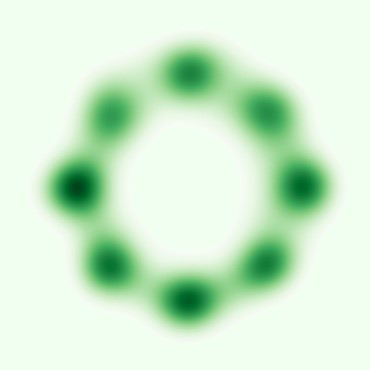
(b) Samples from generator $g_{\theta}(Z)$

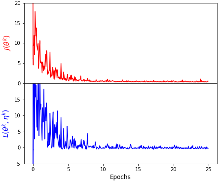
(c) Convergence of the loss functions $J$ and $L$

Figure 4: Samples and loss functions with a mixture of 8 Gaussians, $X\in\mathbb{R}^{2}$, $Z\in\mathbb{R}^{2}$, $N_{g}=5,000$, and $N_{d}=1,000$. The generator accurately learns the sampling distribution, and the loss functions converge to $0$. The code is available at https://github.com/sehyunkwon/Infinite-WGAN.

Proof outline of Lemma 7.

Here, we illustrate the proof in the case of $n=1$. The general $n\geq 1$ case requires similar reasoning but more complicated notation.

First, we define the smooth approximation of $\delta$ by

$$\tilde{\delta}^{\varepsilon}(z)=\frac{C}{\varepsilon^{k}}e^{-\|z/\varepsilon\|^{2}_{2}},$$

where $C$ is a constant (depending on $k$ but not $\varepsilon$) such that

$$\int_{\mathbb{R}^{k}}\tilde{\delta}^{\varepsilon}(z)\,dz=1.$$

We argue that $\tilde{\delta}^{\varepsilon}(z)\approx\delta$ in the sense made precise in Lemma 11 of the appendix.

Next, we approximate $\tilde{\delta}^{\varepsilon}$ with the random feature functions. Using the arguments of (Barron, 1993, Theorem 2) and (Telgarsky, 2020, Section 4.2), we show that there exists a bounded density $m(\kappa)$ and $\kappa_{1}\in\mathbb{R}^{k+1}$ such that $\phi_{1}=\phi(z;\kappa_{1})$ is a nonzero constant function and

$$\tilde{\delta}^{\varepsilon}(z)\approx\theta^{\varepsilon}_{1}\phi_{1}(z)+\int\phi(z;\kappa)\,m(\kappa)\,d\kappa$$

for some $\theta^{\varepsilon}_{1}\in\mathbb{R}$. For large $K>0$,

$$\int\phi(z;\kappa)\,m(\kappa)d\kappa\approx\int\phi(z;\kappa)\,m(\kappa)\mathbf{1}_{\{\|\kappa\|\leq K\}}(\kappa)\,d\kappa,$$

where $\mathbf{1}_{\{\|\kappa\|\leq K\}}$ is the 0-1 indicator function. Write $p(\kappa)$ for the continuous and strictly positive density function of the distribution generating $\kappa$. Then $\sup_{\kappa}\{m(\kappa)\mathbf{1}_{\{\|\kappa\|\leq K\}}(\kappa)/p(\kappa)\}<\infty$, and this allows us to use random feature learning arguments of (Rahimi & Recht, 2008b). By (Rahimi & Recht, 2008b, Lemma 1), there exists a large enough $N_{g}$ such that there exist weights $\{\theta^{\varepsilon}_{i}\}_{i=2}^{N_{g}}$ such that

$$\sum^{N_{g}}_{i=2}\theta^{\varepsilon}_{i}\phi(z;\kappa_{i})\approx\int\phi(z;\kappa)\,m(\kappa)\mathbf{1}_{\{\|\kappa\|\leq K\}}(\kappa)\,d\kappa$$

with probability $1-\zeta$. Finally, we complete the proof by chaining the $\approx$ steps. ∎

We are now ready to state and prove the third main result of this work: our GAN with an finite-width generator and small discriminator has no spurious stationary points within a large ball around the origin.

Theorem 8.

Let $N_{d}\leq n$. Assume (AL), (AG), and (AD). Assume the generator feature functions are generated randomly as in Lemma 7. For any $C>0$ and $\zeta>0$, there exists a large enough $N_{g}\in\mathbb{N}$ such that the following statement holds with probability at least $1-\zeta$: any stationary point $\theta_{\mathrm{s}}\in\mathbb{R}^{N_{g}}$ satisfying $\|\theta_{\mathrm{s}}\|_{1}\leq C$ is a global minimum.

Proof of Theorem 8.

Since $\phi$ is bounded by (AG) and $\|\theta_{\mathrm{s}}\|_{1}$ is bounded, the output of $g_{\theta_{\mathrm{s}}}$ is also bounded, and

$$\sup_{\|\theta_{\mathrm{s}}\|_{1}\leq C}\|g_{\theta_{\mathrm{s}}}(0)\|_{2}<\infty.$$

The (Jacobian kernel point condition), which holds with probability $1$ by Lemma 3, implies

$$C_{1}\stackrel{{\scriptstyle\Delta}}{{=}}\inf_{\|x\|_{2}\leq\left(\underset{{\|\theta_{\mathrm{s}}\|_{1}\leq C}}{\sup}\|g_{\theta_{\mathrm{s}}}(0)\|_{2}\right)}\tau_{\mathrm{min}}(D\Psi(x)^{\intercal})>0,$$

where $\tau_{\mathrm{min}}$ denotes the $N_{d}$-th singular value. We use the fact that $\tau_{\mathrm{min}}(D\Psi(x)^{\intercal})$ is a continuous function of $x$ and the infimum over a compact set of a continuous positive function is positive. (We use $\tau_{\mathrm{min}}$ to denote the minimum singular value, rather than the standard $\sigma_{\mathrm{min}}$ to avoid confusion with the $\sigma$ denoting the activation function.) By (AD),

$$C_{2}\stackrel{{\scriptstyle\Delta}}{{=}}\max_{j=1,\dots,N_{d}}\sup_{x\in\mathbb{R}^{n}}\{\|\nabla\psi_{j}(x)\|+\|\nabla^{2}\psi_{j}(x)\|\}\in(0,\infty)$$

By Lemma 7, there exists a large enough $N_{g}$ such that (Finite universal approximation property) with

$$\varepsilon=\frac{C_{1}q_{Z}(0)}{2C_{2}N_{d}n}$$

holds with probability $1-\zeta$.

Let $\theta_{\mathrm{s}}$ be a stationary point satisfying $\|\theta_{\mathrm{s}}\|_{1}\leq C$. However, assume for contradiction that $J(\theta_{\mathrm{s}})\neq 0$, i.e., $r(\theta_{\mathrm{s}})\neq 0$. Then

$$\frac{\partial}{\partial\theta_{i}}J(\theta_{\mathrm{s}})={\mathbb{E}_{Z}\left[\sum_{j=1}^{N_{d}}r_{j}(\theta_{\mathrm{s}})\nabla\psi_{j}(g_{\theta_{\mathrm{s}}}(Z))^{\intercal}\phi_{i}(Z)\right]}=0$$

for all $1\leq i\leq N_{g}$. Define the normalized residual vector $\hat{r}=(1/\|r\|_{2})r$, and write

$${\mathbb{E}_{Z}\left[\sum_{j=1}^{N_{d}}\hat{r}_{j}(\theta)\nabla\psi_{j}(g_{\theta}(Z))^{\intercal}\phi_{i}(Z)\right]}=0$$ (2)

for all $1\leq i\leq N_{g}$.

Now consider

$$\left|\sum_{j=1}^{N_{d}}\hat{r}_{j}(\theta)\frac{\partial}{\partial x_{l}}\psi_{j}(g_{\theta}(0))q_{Z}(0)\right|$$

$$=\Bigg{|}\mathbb{E}_{Z}\Bigg{[}\underbrace{\sum_{j=1}^{N_{d}}\hat{r}_{j}(\theta)\nabla\psi_{j}(g_{\theta}(Z))^{\intercal}}_{\stackrel{{\scriptstyle\Delta}}{{=}}f(Z)^{\intercal}}\delta^{(l)}(Z)\Bigg{]}\Bigg{|}$$

$$=\left|{\mathbb{E}_{Z}\left[f(Z)^{\intercal}\left(\delta^{(l)}(Z)-\sum_{i=1}^{N_{g}}\theta_{i}^{(l,\varepsilon)}\phi_{i}(z)\right)\right]}\right|$$

$$<\varepsilon\sup_{z\in\mathbb{R}^{k}}\{\|f(z)\|+\|Df(z)\|\}$$

$$\leq\varepsilon\sum_{j=1}^{N_{d}}|\hat{r}_{j}(\theta)|\sup_{x\in\mathbb{R}^{n}}\{\|\nabla\psi_{j}(x)\|+\|\nabla^{2}\psi_{j}(x)\|\}$$

$$\leq\varepsilon C_{2}N_{d},$$

where the first equality follows from the definition of $\delta^{(l)}$, the second equality follows from (2), the first inequality follows from the the (Finite universal approximation property), the second inequality follows from the triangle inequality of the norm, and the third inequality follows from the definition of $C_{2}$ and the fact that the normalized residual satisfies $|\hat{r}_{j}(\theta)|\leq 1$ for all $j$. By summing this result over $1\leq l\leq n$ and using the bound $\|\cdot\|_{2}\leq\|\cdot\|_{1}$, we get

$$\left\|D\Psi(g_{\theta}(0))^{\intercal}\hat{r}(\theta)\right\|_{2}<\varepsilon\frac{C_{2}N_{d}n}{q_{Z}(0)}.$$

Finally, we arrive at

$$C_{1}=C_{1}\|\hat{r}(\theta)\|_{2} \leq\left\|D\Psi(g_{\theta}(0))^{\intercal}\hat{r}(\theta)\right\|_{2}$$

$$<\varepsilon\frac{C_{2}N_{d}n}{q_{Z}(0)}=\frac{C_{1}}{2},$$

which is a contradiction. ∎

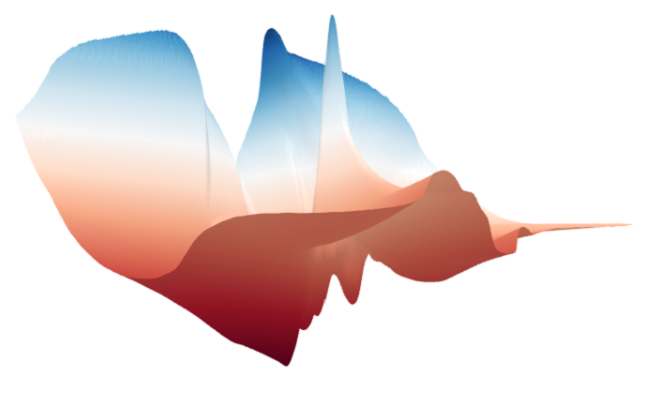
(a) Loss landscape with $N_{g}=2$

(b) Loss landscape with $N_{g}=10$

Figure 5: The landscape of $J(\theta)$ for a mixture of two Gaussians with generator widths $N_{g}=2$ and $N_{g}=10$. The first $N_{g}=2$ example has multiple non-global local minima. The second $N_{g}=10$ example has no spurious stationary points despite the landscape being clearly non-convex. We provide corresponding contour plots in the appendix.

5 Experiments

Figure 6 presents an experiment with a mixture of $8$ Gaussians and $N_{g}=5,000$. The experiments demonstrate the sufficiency of two-layer networks with random features and that the training does not encounter local minima when $N_{g}$ is large.

Figure 5 visualizes the loss landscape with generator widths $N_{g}=2$ and $N_{g}=10$. For the $N_{g}=10$ case, the parameter space was projected down to a 2D space defined by random directions, as recommended by Li et al. (2018b). We observe the landscape becomes more favorable with larger width.

6 Conclusion

In this work, we presented an infinite-width analysis of a WGAN and established that no spurious stationary points exist under certain conditions.

At the same time, however, we point out that the infinite-width analysis does simplify away (hide) some finite phenomena. One such issue we encountered in our experiments was nearly vanishing gradients, which can occur despite the absence of spurious stationary points. A quantitative finite-width analysis establishing explicit bounds may provide an understanding and remedies to such issues and, therefore, is an interesting direction of future work.

Appendix A Omitted proofs

A.1 Proof of Lemma 1

Theorem 9 ((Hornik, 1991, Theorem 1)).

Let $\sigma\colon\mathbb{R}\rightarrow\mathbb{R}$ be bounded and nonconstant and $P\in\mathcal{M}(\mathbb{R}^{k})$ be a finite measure. Then for any $f\in L^{1}(P)$ and $\varepsilon>0$, there exists $N\in\mathbb{N}$ and $\{(\theta_{i},a_{i},b_{i})\in\mathbb{R}\times\mathbb{R}^{k}\times\mathbb{R}\}_{i=1}^{N}$ such that

$$\int_{\mathbb{R}^{k}}\left|\sum_{i=1}^{N}\theta_{i}\sigma(a_{i}^{\intercal}z-b_{i})-f(z)\right|\,dP(z)<\varepsilon.$$

To clarify, $f\colon\mathbb{R}^{k}\rightarrow\mathbb{R}$ in (Hornik, 1991, Theorem 1).

Proof of Lemma 1.

Let $f\colon\mathbb{R}^{k}\rightarrow\mathbb{R}^{n}$ such that ${\mathbb{E}_{Z}\left[\|f(Z)\|_{2}\right]}<\infty$. By (AG), $\sigma_{\mathrm{g}}$ is a bounded nonconstant function. For $l=1,\dots,n$, Theorem 9 provides us with $N_{l}\in\mathbb{N}$ and $\{(\theta_{i}^{(l)},a_{i}^{(l)},b_{i}^{(l)})\in\mathbb{R}\times\mathbb{R}^{k}\times\mathbb{R}\}_{i=1}^{N_{l}}$ such that

$$h_{l}(z)=\sum_{i=1}^{N_{l}}\theta_{i}^{(l)}\sigma_{\mathrm{g}}((a_{i}^{(l)})^{\intercal}z-b_{i}^{(l)})$$

satisfies

$$\int_{\mathbb{R}^{k}}\left|h_{l}(z)-f_{l}(z)\right|\,q_{Z}(z)dz<\frac{\varepsilon}{2n},$$ (3)

where $f_{l}(z)$ is the $l$-th coordinate of $f(z)\in\mathbb{R}^{n}$ for $l=1,\dots,n$. Let $\ell_{g}=\lim_{r\to-\infty}\sigma_{g}(r)$. Let

$$A^{(l)}_{i}=\begin{bmatrix}0\\ \vdots\\ 0\\ (a_{i}^{(l)})^{\intercal}\\ 0\\ \vdots\\ 0\end{bmatrix}\leftarrow\text{$l$-th row},\qquad\mathbf{b}^{(l),r}_{i}=\begin{bmatrix}r\\ \vdots\\ r\\ b_{i}^{(l)}\\ r\\ \vdots\\ r\end{bmatrix},\qquad e_{-l}=\begin{bmatrix}1\\ \vdots\\ 1\\ 0\\ 1\\ \vdots\\ 1\end{bmatrix}\leftarrow\text{on $l$-th coordinates}$$

and

$$\tilde{f}^{(l),r}(z)=-\left(\sum_{i=1}^{N_{l}}\theta_{i}^{(l)}\right)\ell_{g}e_{-l}+\sum_{i=1}^{N_{l}}\theta_{i}^{(l)}\sigma_{\mathrm{g}}(A_{i}^{(l)}z-\mathbf{b}^{(l),r}_{i}).$$

Then, for each $l=1,\dots,n$, we have $\tilde{f}^{(l),r}_{j}=\sum_{i=1}^{N_{l}}\theta_{i}^{(l)}(\sigma_{g}(-r)-\ell_{g})\to 0$ as $r\to\infty$ if $j\neq l$, while $\tilde{f}^{(l),r}_{l}=h_{l}(z)$. Because $\sigma_{g}$ is bounded, by Lebesgue’s dominated convergence theorem, we obtain

$$\lim_{r\rightarrow\infty}\int_{\mathbb{R}^{k}}\left\|\begin{bmatrix}h_{1}(z)\\ \vdots\\ h_{n}(z)\end{bmatrix}-\sum^{n}_{l=1}\tilde{f}^{(l),r}(z)\right\|_{1}\,q_{Z}(z)dz=0.$$

Therefore, there exists a large enough $r_{\mathrm{big}}>0$ such that

$$\int_{\mathbb{R}^{k}}\left\|\begin{bmatrix}h_{1}(z)\\ \vdots\\ h_{n}(z)\end{bmatrix}-\sum^{n}_{l=1}\tilde{f}^{(l),r_{\mathrm{big}}}(z)\right\|_{1}\,q_{Z}(z)dz<\frac{\varepsilon}{2}$$

and we conclude with (3) that

$$\int_{\mathbb{R}^{k}}\left\|f(z)-\sum^{n}_{l=1}\tilde{f}^{(l),r_{\mathrm{big}}}(z)\right\|_{1}\,q_{Z}(z)dz<\varepsilon.$$

Note that

$$\sum^{n}_{l=1}\tilde{f}^{(l),r_{\mathrm{big}}}(z)\in\overline{\mathrm{span}}({\cal G}).$$

Therefore, using the bound $\|\cdot\|_{2}\leq\|\cdot\|_{1}$, we get

$$\int_{\mathbb{R}^{k}}\left\|f(z)-\sum^{n}_{l=1}\tilde{f}^{(l),r_{\mathrm{big}}}(z)\right\|_{2}\,q_{Z}(z)dz<\varepsilon.$$

∎

A.2 Proof of Lemma 2

Proof of Lemma 2.

Because $h$ is bounded and $q_{Z}(z)\,dz$ is a probability measure, we have ${\mathbb{E}_{Z}\left[\|h(Z)\|_{2}\right]}<\infty$. Therefore, for any $\varepsilon>0$, there exists $\theta_{\varepsilon}$ such that ${\mathbb{E}_{Z}\left[\left\|g_{\theta_{\varepsilon}}(Z)-h(Z)\right\|_{2}\right]}<\varepsilon$. Observe that

$$\mathbb{E}_{Z}\left[g_{\theta_{\varepsilon}}^{\intercal}(Z)h(Z)\right] =\int_{\mathbb{R}^{k}}\int_{\mathbb{R}^{p}}h^{\intercal}(z)\phi(z;\kappa)\,d\theta_{\varepsilon}(\kappa)\,q_{Z}(z)\,dz$$

$$=\int_{\mathbb{R}^{p}}\int_{\mathbb{R}^{k}}h^{\intercal}(z)\phi(z;\kappa)q_{Z}(z)\,dz\,d\theta_{\varepsilon}(\kappa)$$

$$=\int{\mathbb{E}_{Z}\left[h^{\intercal}(Z)\phi(Z;\kappa)\right]}\,d\theta_{\varepsilon}(\kappa)=0.$$

Here the change in the order of integration is valid because $\phi(z;\kappa)=\sigma_{\mathrm{g}}(\kappa_{w}z+\kappa_{b})\leq\|\sigma_{\mathrm{g}}\|_{\infty}$ and the total mass of $\theta_{\varepsilon}$ is finite, so that

$$\int_{\mathbb{R}^{k}}\int_{\mathbb{R}^{p}}\left\|h^{\intercal}(z)\phi(z;\kappa)\right\|_{2}\,d\theta_{\varepsilon}(\kappa)\,q_{Z}(z)\,dz\leq n\|h\|_{\infty}\left\|\sigma_{\mathrm{g}}\right\|_{\infty}\theta_{\varepsilon}\left(\mathbb{R}^{p}\right)<\infty.$$

To clarify, the $\|\cdot\|_{\infty}$ for $\|\sigma_{\mathrm{g}}\|_{\infty}$ is the standard supremum norm for $L^{\infty}$ spaces while $\|h\|_{\infty}=\max_{1\leq i\leq n}\|h_{i}\|_{\infty}$ where $h_{i}(z)$ is the $i$-th coordinate of $h(z)\in\mathbb{R}^{n}$. Finally, we have

$$\mbox{$\mathbb{E}_{Z}\left[\|h(Z)\|_{2}^{2}\right]$}={\mathbb{E}_{Z}\left[h^{\intercal}(Z)\left(h(Z)-g_{\theta_{\varepsilon}}(Z)\right)\right]} \leq\|h\|_{\infty}{\mathbb{E}_{Z}\left[\left\|h(Z)-g_{\theta_{\varepsilon}}(Z)\right\|_{1}\right]}$$

$$\leq\|h\|_{\infty}{\mathbb{E}_{Z}\left[\sqrt{n}\left\|h(Z)-g_{\theta_{\varepsilon}}(Z)\right\|_{2}\right]}<\varepsilon\sqrt{n}\|h\|_{\infty}.$$

To clarify, $\left\|h(Z)-g_{\theta_{\varepsilon}}(Z)\right\|_{1}$ denotes the $\ell^{1}$ norm on the vector in $\mathbb{R}^{n}$ for each $z$. Now by letting $\varepsilon\rightarrow 0$, we have

$$0={\mathbb{E}_{Z}\left[\|h(Z)\|_{2}^{2}\right]}=\int\|h(z)\|_{2}^{2}\,q_{Z}(z)\,dz.$$

Since $q_{Z}$ is continuous and positive everywhere, we conclude that $h(z)=0$ for all $z\in\mathbb{R}^{k}$. ∎

A.3 Proof of Lemma 5

Theorem 10 ((Sussmann, 1992, Lemma 1)).

Let $\sigma=\tanh$. Assume

$$C_{0}+\sum^{N}_{j=1}\eta_{j}\sigma(a_{j}^{\intercal}x+b_{j})=C$$

for all $x\in\mathbb{R}^{n}$, where $\eta_{j}\neq 0$ and $a_{j}\neq 0$ for $1\leq j\leq N$. If there exists no distinct indices $i$ and $j$ such that $(a_{i},b_{i})=\pm(a_{j},b_{j})$, then $N=0$ (the sum vanishes) and $C_{0}=C$.

Proof of Lemma 5.

First consider the case where $\sigma=\tanh$. With probability $1$, the condition of Theorem 10 holds, and

$$F(x)\stackrel{{\scriptstyle\Delta}}{{=}}\sum_{j=1}^{N_{d}}\eta_{j}\psi_{j}(x)$$

with $\eta\neq 0$ is not constant. Since $\sigma\colon\mathbb{R}\rightarrow\mathbb{R}$ is analytic on $\mathbb{R}$, it has a power series expansion

$$\sigma(t)=\sum_{\nu=0}^{\infty}s_{\nu}\,t^{\nu}.$$

Suppose that $0\neq\eta\in\bigcap_{x\in B}\ker(D\Psi(x)^{\intercal})$. Then

$$\sum_{j=1}^{N_{d}}\eta_{j}\nabla\psi_{j}(x)\equiv 0$$

for $x\in B$, and

$$F(x)\stackrel{{\scriptstyle\Delta}}{{=}}\sum_{j=1}^{N_{d}}\eta_{j}\psi_{j}(x)=\sum_{j=1}^{N_{d}}\eta_{j}\sum_{\nu=0}^{\infty}s_{\nu}(a_{j}^{\intercal}x+b_{j})^{\nu}$$

is constant for $x\in B$. Fix any $x_{0}\in B$ and $u\in\mathbb{R}^{n}$. Let $\alpha_{j}=a_{j}^{\intercal}u$ and $\beta_{j}=a_{j}^{\intercal}x_{0}+b_{j}$. Then for $x_{u}(t)\stackrel{{\scriptstyle\Delta}}{{=}}x_{0}+tu$,

$$F(x_{u}(t)) =\sum_{j=1}^{N_{d}}\eta_{j}\sum_{\nu=0}^{\infty}s_{\nu}(t\alpha_{j}+\beta_{j})^{\nu}$$

$$=\sum_{j=1}^{N_{d}}\eta_{j}\sum_{\nu=0}^{\infty}s_{\nu}\sum_{m=0}^{\nu}\binom{\nu}{m}(\alpha_{j}t)^{m}\beta_{j}^{\nu-m}$$

$$=\sum_{m=0}^{\infty}\left(\sum_{j=1}^{N_{d}}\sum_{\nu\geq m}\eta_{j}s_{\nu}\binom{\nu}{m}\alpha_{j}^{m}\beta_{j}^{\nu-m}\right)t^{m}$$

$$\stackrel{{\scriptstyle\Delta}}{{=}}F_{0}+\sum_{m=1}^{\infty}F_{m}t^{m}$$

is constant within $t\in(-\varepsilon,\varepsilon)$ for some $\varepsilon>0$. (Order of summations can be freely interchanged because power series for $\sigma$ are absolutely convergent for any choice of $t$.) But then $F_{m}$ must be zero for all $m\geq 1$, since $0=\frac{d^{m}}{dt^{m}}\sum_{j=1}^{N_{d}}\eta_{j}\psi_{j}(x_{u}(0))=m!\,F_{m}$. Therefore, in fact, $F(x_{u}(t))\equiv F_{0}$ for all $t\in\mathbb{R}$, and $F_{0}=F(x_{0})$ does not depend on $u$. That is, $F$ is a constant function on $\mathbb{R}^{n}$. This implies that $\eta=0$, which contradicts the assumption $\eta\neq 0$.

We extend the conclusion to the sigmoid function by noting that

$$\frac{1}{1+e^{-r}}=\frac{\tanh(r/2)+1}{2},$$

i.e., the sigmoid function is obtained by scaling the input of $\tanh$, adding a constant, and scaling the output. ∎

A.4 Proof of Lemma 7

Recall that we defined

$$\tilde{\delta}^{\varepsilon}(z)=\frac{\pi^{-k/2}}{\varepsilon^{k}}e^{-\|z/\varepsilon\|_{2}^{2}},$$

so that $\int_{\mathbb{R}^{k}}\tilde{\delta}^{\varepsilon}(z)\,dz=1$ for all $\varepsilon>0$.

Lemma 11.

Assume (AL). There exists a constant $C_{\delta}$ depending only on $k$ but not on $\varepsilon>0$ such that

$$\left|\mathbb{E}_{Z}\left[\left(\tilde{\delta}^{\varepsilon}(Z)-\delta(Z)\right)f(Z)\right]\right|<C_{\delta}\,\varepsilon\sup_{z\in\mathbb{R}^{k}}\left(|f(z)|+\|\nabla f(z)\|\right)$$

for all differentiable $f\colon\mathbb{R}^{k}\rightarrow\mathbb{R}$ such that $\sup_{z\in\mathbb{R}^{k}}\left(|f(z)|+\|\nabla f(z)\|\right)<\infty$. Here $\|\cdot\|$ denotes the operator norm, which coincides with the vector $\ell^{2}$ norm on $\mathbb{R}^{k}$.

Proof.

Let $M=\|f\|_{\infty}$, $L_{f}=\sup_{z\in\mathbb{R}^{k}}\|\nabla f(z)\|$ and let $L_{Z}$ be the Lipschitz constant of $q_{Z}(z)$. Then for any $z\in\mathbb{R}^{k}$,

$$|f(z)q_{Z}(z)-f(0)q_{Z}(0)|\leq|f(z)||q_{Z}(z)-q_{z}(0)|+|f(z)-f(0)|q_{Z}(0)\leq ML_{Z}\|z\|+L_{f}\|z\|q_{Z}(0).$$

Integrating both sides over $z\in\mathbb{R}^{k}$ with respect to $\tilde{\delta}^{\varepsilon}(z)\,dz$ gives

$$\int_{\mathbb{R}^{k}}|f(z)q_{Z}(z)-f(0)q_{Z}(0)|\,\tilde{\delta}^{\varepsilon}(z)\,dz \leq\int_{\mathbb{R}^{k}}(ML_{Z}+L_{f}q_{Z}(0))\|z\|\tilde{\delta}^{\varepsilon}(z)\,dz$$

$$=\int_{\mathbb{R}^{k}}(ML_{Z}+L_{f}q_{Z}(0))\frac{\pi^{-k/2}}{\varepsilon^{k}}\|z\|e^{-\|z/\varepsilon\|_{2}^{2}}\,dz.$$

Using change of variables, we rewrite and bound the last integral as

$$(ML_{Z}+L_{f}q_{Z}(0))\pi^{-k/2}\varepsilon\int_{\mathbb{R}^{k}}\|z\|e^{-\|z\|_{2}^{2}}\,dz \leq\max\{L_{Z},q_{Z}(0)\}\pi^{-k/2}\left(\int_{\mathbb{R}^{k}}\|z\|e^{-\|z\|_{2}^{2}}\,dz\right)\varepsilon(M+L_{f})$$

$$\leq 2\max\{L_{Z},q_{Z}(0)\}\pi^{-k/2}\left(\int_{\mathbb{R}^{k}}\|z\|e^{-\|z\|_{2}^{2}}\,dz\right)\varepsilon\sup_{z\in\mathbb{R}^{k}}\left(|f(z)|+\|Df(z)\|\right),$$

which shows that

$$\left|\mathbb{E}_{Z}\left[\left(\tilde{\delta}^{\varepsilon}(Z)-\delta(Z)\right)f(Z)\right]\right| \leq\int_{\mathbb{R}^{k}}|f(z)q_{Z}(z)-f(0)q_{Z}(0)|\tilde{\delta}^{\varepsilon}(z)\,dz$$

$$\leq C_{\delta}\,\varepsilon\sup_{z\in\mathbb{R}^{k}}\left(|f(z)|+\|Df(z)\|\right)$$

where

$$C_{\delta}=2\max\{L_{Z},q_{Z}(0)\}\pi^{-k/2}\left(\int_{\mathbb{R}^{k}}\|z\|e^{-\|z\|_{2}^{2}}\,dz\right).$$

∎

Lemma 12.

(Abramowitz & Stegun, 1972, p. 302) Denote by ${\cal F}[\cdot]$ be the Fourier transform operator. Then

$${\cal F}[\tilde{\delta}^{\varepsilon}](\omega)=e^{-\pi^{2}\varepsilon^{2}\|\omega\|^{2}}.$$

In particular, ${\cal F}[\tilde{\delta}^{\varepsilon}](\omega)$ is bounded, and

$$\int_{\mathbb{R}^{k}}{\cal F}[\tilde{\delta}^{\varepsilon}](\omega)\,d\omega<\infty,$$

$$\int_{\mathbb{R}^{k}}\|\omega\|\,{\cal F}[\tilde{\delta}^{\varepsilon}](\omega)\,d\omega<\infty.$$

We first provide a proof when $n=1$, which conveys all important ideas of the proof. Although the general case involves significantly more complicated notations, it does not essentially differ from the simpler case.

Proof for the case $n=1$.

Let $\varepsilon>0$ be given.

Step 1. Approximate $\delta(z)$ with $\tilde{\delta}^{\varepsilon}(z)$ in the sense of Lemma 11.

Step 2. Approximate $\tilde{\delta}^{\varepsilon}(z)$ with an infinite combination of functions in ${\cal G}$.

Because both $\tilde{\delta}^{\varepsilon}$ and ${\cal F}[\tilde{\delta}^{\varepsilon}]$ are real-valued and positive, using the inverse Fourier transform, we can write

$$\tilde{\delta}^{\varepsilon}(z)-\tilde{\delta}^{\varepsilon}(0) =\mathrm{Re}\int\left(e^{2\pi i\omega^{\intercal}z}-1\right){\cal F}[\tilde{\delta}^{\varepsilon}](\omega)\,d\omega=\int\left(\cos\left(2\pi\omega^{\intercal}z\right)-1\right){\cal F}[\tilde{\delta}^{\varepsilon}](\omega)\,d\omega$$ (4)

for any $z\in\mathbb{R}^{k}$. Note that by Lemma 12, the integral (4) is always well-defined.

Fix a large $R>0$ satisfying

$$\int_{\|z\|>R}q_{Z}(z)\,dz<\frac{\pi^{k/2}\varepsilon^{k+1}}{2}.$$

Following (Telgarsky, 2020, Section 4.2), for $\|z\|\leq R$, the cosine term in (4) can be rewritten as

$$\cos\left(2\pi\omega^{\intercal}z\right)-1$$

$$=\int_{0}^{\omega^{\intercal}z}-2\pi\sin(2\pi b)\,db$$

$$=\int_{0}^{R\|\omega\|}-2\pi\,\mathbf{1}_{\{\omega^{\intercal}z-b\geq 0\}}(z)\,\sin(2\pi b)\,db+\int_{-R\|\omega\|}^{0}2\pi\,\mathbf{1}_{\{\omega^{\intercal}z-b\leq 0\}}(z)\,\sin(2\pi b)\,db.$$ (5)

Let $u_{g}=\lim_{r\to\infty}\sigma_{g}(r)$ and $\ell_{g}=\lim_{r\to-\infty}\sigma_{g}(r)$. Then by (AG), we have

$$\mathbf{1}_{\{r\geq 0\}}(r)=\lim_{\tau\downarrow 0}\frac{1}{u_{g}-\ell_{g}}\left(\sigma_{g}\left(\frac{r}{\tau}\right)-\ell_{g}\right)$$

for $r\neq 0$. Hence we can approximate the step function terms in (5) using $\sigma_{g}$:

$$\int_{0}^{R\|\omega\|}\lim_{\tau\downarrow 0}-\frac{2\pi}{u_{g}-\ell_{g}}\left(\sigma_{g}\left(\frac{\omega^{\intercal}z-b}{\tau}\right)-\ell_{g}\right)\sin(2\pi b)\,db+\int_{-R\|\omega\|}^{0}\lim_{\tau\downarrow 0}\frac{2\pi}{u_{g}-\ell_{g}}\left(\sigma_{g}\left(\frac{-\omega^{\intercal}z+b}{\tau}\right)-\ell_{g}\right)\sin(2\pi b)\,db.$$ (6)

Plugging (6) into (4), we obtain

$$\tilde{\delta}^{\varepsilon}(z)-\tilde{\delta}^{\varepsilon}(0)$$

$$\begin{aligned} &=\int\int_{0}^{R\|\omega\|}\lim_{\tau\downarrow 0}-\frac{2\pi}{u_{g}-\ell_{g}}\left(\sigma_{g}\left(\frac{\omega^{\intercal}z-b}{\tau}\right)-\ell_{g}\right)\sin(2\pi b)\,{\cal F}[\tilde{\delta}^{\varepsilon}](\omega)\,db\,d\omega\\ &\quad+\int\int_{-R\|\omega\|}^{0}\lim_{\tau\downarrow 0}\frac{2\pi}{u_{g}-\ell_{g}}\left(\sigma_{g}\left(\frac{-\omega^{\intercal}z+b}{\tau}\right)-\ell_{g}\right)\sin(2\pi b)\,{\cal F}[\tilde{\delta}^{\varepsilon}](\omega)\,db\,d\omega\end{aligned}$$ (7)

for $\|z\|\leq R$.

Observe that because $\sigma_{g}$ is bounded and by Lemma 12, for any $\tau>0$ and $z\in\mathbb{R}^{k}$,

$$\int\int_{0}^{R\|\omega\|}\left|\frac{2\pi}{u_{g}-\ell_{g}}\left(\sigma_{g}\left(\frac{\omega^{\intercal}z-b}{\tau}\right)-\ell_{g}\right)\sin(2\pi b)\,{\cal F}[\tilde{\delta}^{\varepsilon}](\omega)\right|\,db\,d\omega\leq\int\frac{2\pi\left(\|\sigma_{g}\|_{\infty}+\ell_{g}\right)}{u_{g}-\ell_{g}}R\|\omega\|\,{\cal F}[\tilde{\delta}^{\varepsilon}]\,d\omega<\infty.$$

Therefore, by Lebesgue’s dominated convergence theorem, we can freely change the order of integration and limit in (7). Using this fact, and applying change of variables, we can rewrite $\tilde{\delta}^{\varepsilon}(z)$ as

$$\tilde{\delta}^{\varepsilon}(z) =\tilde{\delta}^{\varepsilon}(0)+\lim_{\tau\downarrow 0}\int\int_{0}^{R\|\omega\|}-\frac{2\pi}{u_{g}-\ell_{g}}\left(\sigma_{g}\left(\frac{\omega^{\intercal}z-b}{\tau}\right)-\ell_{g}\right)\sin(2\pi b)\,{\cal F}[\tilde{\delta}^{\varepsilon}](\omega)\,db\,d\omega$$

$$\quad\quad\quad\,\,\,+\lim_{\tau\downarrow 0}\int\int_{-R\|\omega\|}^{0}\frac{2\pi}{u_{g}-\ell_{g}}\left(\sigma_{g}\left(\frac{-\omega^{\intercal}z+b}{\tau}\right)-\ell_{g}\right)\sin(2\pi b)\,{\cal F}[\tilde{\delta}^{\varepsilon}](\omega)\,db\,d\omega$$

$$=\theta^{\varepsilon}_{1}\phi(z;\kappa_{1})+\lim_{\tau\downarrow 0}\int\int_{-R\|\omega\|}^{0}-\frac{2\pi\tau^{k+1}}{u_{g}-\ell_{g}}\sigma_{g}\left(\omega^{\intercal}z+b\right)\sin(-2\pi\tau b)\,{\cal F}[\tilde{\delta}^{\varepsilon}](\tau\omega)\,db\,d\omega$$

$$\quad\quad\quad\,\,\,+\lim_{\tau\downarrow 0}\int\int_{-R\|\omega\|}^{0}\frac{2\pi\tau^{k+1}}{u_{g}-\ell_{g}}\sigma_{g}\left(\omega^{\intercal}z+b\right)\sin(2\pi\tau b)\,{\cal F}[\tilde{\delta}^{\varepsilon}](-\tau\omega)\,db\,d\omega$$

$$=\theta^{\varepsilon}_{1}\phi(z;\kappa_{1})+\lim_{\tau\downarrow 0}\int_{\mathbb{R}^{k}\times\mathbb{R}}\phi(z;\kappa)m_{\tau}(\kappa)\,d\kappa$$

for $\|z\|\leq R$. We specify the notations that were newly introduced. First, we denoted $\kappa=(\omega,b)$, so that $\phi(z;\kappa)=\sigma_{g}(\omega^{\intercal}z+b)$ (note that because we have assumed $n=1$, the generator parameter has dimension $k+1$), and $d\kappa$ is the Lebesgue measure on $\mathbb{R}^{k}\times\mathbb{R}$. Next, we set $\kappa_{1}=(0,b_{1})$ with some fixed $b_{1}\in\mathbb{R}$ satisfying $\phi(z;\kappa_{1})\equiv\sigma_{g}(b_{1})\neq 0$ and

$$\theta^{\varepsilon}_{1} =\frac{1}{\sigma_{g}(b_{1})}\left(\tilde{\delta}^{\varepsilon}(0)+\int\int_{0}^{R\|\omega\|}\frac{2\pi\ell_{g}}{u_{g}-\ell_{g}}\sin(2\pi b){\cal F}[\tilde{\delta}^{\varepsilon}](\omega)\,db\,d\omega-\int\int_{-R\|\omega\|}^{0}\frac{2\pi\ell_{g}}{u_{g}-\ell_{g}}\sin(2\pi b){\cal F}[\tilde{\delta}^{\varepsilon}](\omega)\,db\,d\omega\right)\in\mathbb{R}.$$

Finally, we define the density function $m_{\tau}(\kappa)$ as

$$m_{\tau}(\kappa) =\frac{2\pi\tau^{k+1}}{u_{g}-\ell_{g}}\left(-\sin(-2\pi\tau b)\,{\cal F}[\tilde{\delta}^{\varepsilon}](\tau\omega)\,\mathbf{1}_{\{-R\|\omega\|\leq b\leq 0\}}(\kappa)+\sin(2\pi\tau b)\,{\cal F}[\tilde{\delta}^{\varepsilon}](-\tau\omega)\,\mathbf{1}_{\{-R\|\omega\|\leq b\leq 0\}}(\kappa)\right)$$

$$=\frac{4\pi\tau^{k+1}}{u_{g}-\ell_{g}}e^{-\pi^{2}\varepsilon^{2}\tau^{2}\|\omega\|^{2}}\sin(2\pi\tau b)\,\mathbf{1}_{\{-R\|\omega\|\leq b\leq 0\}}(\kappa),$$ (8)

where we used Lemma 12 to obtain the second equality.

Now we bound the error in using the expression (5) in the case $\|z\|>R$. Observe that

$$\cos(2\pi\omega^{\intercal}z)-1-\int_{0}^{R\|\omega\|}-2\pi\,\mathbf{1}_{\{\omega^{\intercal}z-b\geq 0\}}(z)\,\sin(2\pi b)\,db+\int_{-R\|\omega\|}^{0}2\pi\,\mathbf{1}_{\{\omega^{\intercal}z-b\leq 0\}}(z)\,\sin(2\pi b)\,db$$

$$\quad=\left(\cos(2\pi\omega^{\intercal}z)-\cos(2\pi R\|\omega\|)\right)\mathbf{1}_{\{|\omega^{\intercal}z|>R\|\omega\|\}}(\omega),$$

and thus

$$\tilde{\delta}^{\varepsilon}(z)-\theta_{1}^{\varepsilon}\phi(z;\kappa_{1})-\lim_{\tau\downarrow 0}\int_{\mathbb{R}^{k}\times\mathbb{R}}\phi(z;\kappa)m_{\tau}(\kappa)\,d\kappa=\int_{\{\omega\,|\,|\omega^{\intercal}z|>R\|\omega\|\}}\left(\cos(2\pi\omega^{\intercal}z)-\cos(2\pi R\|\omega\|)\right){\cal F}[\tilde{\delta}^{\varepsilon}](\omega)\,d\omega$$ (9)

for all $z\in\mathbb{R}^{k}$. The defining equation (8) shows that $m_{\tau}$ is bounded and $m_{\tau}\in L^{1}(d\kappa)$ with

$$\int_{\mathbb{R}^{k}\times\mathbb{R}}\left|m_{\tau}(\kappa)\right|\,d\kappa\leq\frac{4\pi R}{u_{g}-\ell_{g}}\int_{\mathbb{R}^{k}}\tau^{k}\|\tau\omega\|e^{-\pi^{2}\varepsilon^{2}\|\tau\omega\|^{2}}\,d\omega=\frac{4\pi R}{u_{g}-\ell_{g}}\int_{\mathbb{R}^{k}}\|\omega\|e^{-\pi^{2}\varepsilon^{2}\|\omega\|^{2}}\,d\omega.$$

Therefore, the family

$$\left\{\tilde{\delta}^{\varepsilon}(z)-\theta^{\varepsilon}_{1}\phi(z;\kappa_{1})-\int_{\mathbb{R}^{k}\times\mathbb{R}}\phi(z;\kappa)f(z)m_{\tau}(\kappa)\,d\kappa\right\}_{\tau>0}$$

is uniformly bounded. Applying the dominated convergence theorem to the pointwise convergence result (9) with respect to the probability measure $q_{Z}(z)\,dz$, we obtain

$$\lim_{\tau\downarrow 0}\mathbb{E}_{Z}\left[\left|\tilde{\delta}^{\varepsilon}(Z)-\theta^{\varepsilon}_{1}\phi(Z;\kappa_{1})-\int_{\mathbb{R}^{k}\times\mathbb{R}}\phi(Z;\kappa)m_{\tau}(\kappa)\,d\kappa\right|\right]$$

$$=\mathbb{E}_{Z}\left[\left|\int_{\{\omega\,|\,|\omega^{\intercal}Z|>R\|\omega\|\}}\left(\cos(2\pi\omega^{\intercal}Z)-\cos(2\pi R\|\omega\|)\right){\cal F}[\tilde{\delta}^{\varepsilon}](\omega)\,d\omega\right|\right]$$

$$\leq\mathbb{E}_{Z}\left[\int_{\{\omega\,|\,|\omega^{\intercal}Z|>R\|\omega\|\}}2{\cal F}[\tilde{\delta}^{\varepsilon}](\omega)\,d\omega\right]$$

$$\leq\mathbb{E}_{Z}\left[\mathbf{1}_{\{\|z\|>R\}}(Z)\int_{\mathbb{R}^{k}}2{\cal F}[\tilde{\delta}^{\varepsilon}](\omega)\,d\omega\right]$$

$$=\left(\int_{\{\|z\|>R\}}q_{Z}(z)\,dz\right)\left(\int_{\mathbb{R}^{k}}2{\cal F}[\tilde{\delta}^{\varepsilon}](\omega)\,d\omega\right)<\frac{\pi^{k/2}\varepsilon^{k+1}}{2}\frac{2}{\pi^{k/2}\varepsilon^{k}}=\varepsilon.$$

Step 3. Approximate the integral over $\mathbb{R}^{k}\times\mathbb{R}$ by an integral over a ball of finite radius.

We fix some $\tau=\tau(\varepsilon)$ satisfying $\mathbb{E}_{Z}\left[\left|\tilde{\delta}^{\varepsilon}(Z)-\theta^{\varepsilon}_{1}\phi(Z;\kappa_{1})-\int_{\mathbb{R}^{k}\times\mathbb{R}}\phi(Z;\kappa)m_{\tau}(\kappa)\,d\kappa\right|\right]<2\varepsilon$. Because $\sigma_{g}$ is bounded and $m_{\tau}\in L^{1}(d\kappa)$, there exists $K>0$ large enough so that

$$\int_{\|\kappa\|>K}|m_{\tau}(\kappa)|\,d\kappa<\frac{\varepsilon}{\|\sigma_{g}\|_{\infty}}.$$

Then for any bounded continuous function $f:\mathbb{R}^{k}\to\mathbb{R}$ we have

$$\mathbb{E}_{Z}\left[\left|\tilde{\delta}^{\varepsilon}(Z)f(Z)-\theta^{\varepsilon}_{1}\phi(Z;\kappa_{1})f(Z)-\int_{\|\kappa\|\leq K}\phi(Z;\kappa)f(Z)m_{\tau}(\kappa)\,d\kappa\right|\right]$$

$$\leq\mathbb{E}_{Z}\left[\left|\tilde{\delta}^{\varepsilon}(Z)f(Z)-\theta^{\varepsilon}_{1}\phi(Z;\kappa_{1})f(Z)-\int_{\mathbb{R}^{k}\times\mathbb{R}}\phi(Z;\kappa)f(Z)m_{\tau}(\kappa)\,d\kappa\right|\right]$$

$$\quad\quad+\mathbb{E}_{Z}\left[\int_{\|\kappa\|>K}\left|\phi(Z;\kappa)f(Z)m_{\tau}(\kappa)\right|\,d\kappa\right]$$

$$\leq 2\varepsilon\|f\|_{\infty}+\|\sigma_{g}\|_{\infty}\|f\|_{\infty}\mathbb{E}_{Z}\left[\int_{\|\kappa\|>K}|m_{\tau}(\kappa)|\,d\kappa\right]\leq 3\varepsilon\|f\|_{\infty}.$$

Step 4. Approximate the integral over a finite ball by a finite linear combination of random functions in ${\cal G}$.

Define

$$m_{\tau,K}(\kappa)=\begin{cases}m_{\tau}(\kappa)&\text{if }\|\kappa\|\leq K,\\ 0&\text{otherwise}.\end{cases}$$

Denote by $p(\kappa)$ the strictly positive continuous density function from which we randomly sample the generator parameters.

Note that we have

$$C_{K}\stackrel{{\scriptstyle\Delta}}{{=}}\sup_{\kappa}\left|\frac{m_{\tau,K}(\kappa)}{p(\kappa)}\right|<\infty$$

because $\|m_{\tau}\|_{\infty}<\infty$ and $1/p(\kappa)$ is bounded over a compact set.

Now, rewrite the integral from Step 3 as

$$\int_{\|\kappa\|\leq K}\phi\left(z;\kappa\right)\,m_{\tau}(\kappa)\,d\kappa=\int\phi\left(z;\kappa\right)\frac{m_{\tau,K}(\kappa)}{p(\kappa)}\,p(\kappa)\,d\kappa.$$

We will show that if we sample $\kappa_{2},\dots,\kappa_{N_{g}}$ (IID) according to $p(\kappa)$, then for sufficiently large $N_{g}$,

$$\int\phi\left(Z;\kappa\right)\frac{m_{\tau,K}(\kappa)}{p(\kappa)}\,p(\kappa)\,d\kappa\approx\frac{1}{N_{g}-1}\sum_{i=2}^{N_{g}}\phi(Z;\kappa_{i})\frac{m_{\tau,K}(\kappa_{i})}{p(\kappa_{i})}$$

with high probability over $\kappa_{2},\dots,\kappa_{N_{g}}$. (The indexing begins with $i=2$ because $\kappa_{1}$ is reserved for the constant function.) When we draw each $\kappa_{i}$, we are in fact sampling the corresponding function

$$h_{i}\stackrel{{\scriptstyle\Delta}}{{=}}\frac{m_{\tau,K}(\kappa_{i})}{p(\kappa_{i})}\phi(\cdot;\kappa_{i})\in{\cal H}\stackrel{{\scriptstyle\Delta}}{{=}}L^{2}(q_{Z}(z)\,dz).$$

Indeed, $h_{i}$ are uniformly bounded with $\|h_{i}\|_{\infty}\leq\|\sigma_{g}\|_{\infty}C_{K}$ for all $i=2,\dots,N_{g}$, which implies $\|h_{i}\|_{\cal H}\leq\|\sigma_{g}\|_{\infty}C_{K}$. That is, $\frac{m_{\tau,K}(\kappa)}{p(\kappa)}\phi(\cdot;\kappa)$ is a bounded random variable with random realizations in ${\cal H}$. Also, we have

$$\mathbb{E}_{\kappa\sim p(\kappa)}\left[\frac{m_{\tau,K}(\kappa)}{p(\kappa)}\phi(\cdot;\kappa)\right]=\int\phi(\cdot;\kappa)\frac{m_{\tau,K}(\kappa)}{p(\kappa)}p(\kappa)\,d\kappa=\int_{\|\kappa\|\leq K}\phi(\cdot;\kappa)\,m_{\tau}(\kappa)\,d\kappa.$$

Therefore, applying the McDiarmid-type bound from (Rahimi & Recht, 2007, Lemma 4), we get

$$\begin{aligned} \left\|\frac{1}{N_{g}-1}\sum_{i=2}^{N_{g}}h_{i}-\mathbb{E}_{\kappa\sim p(\kappa)}\left[\frac{m_{\tau,K}(\kappa)}{p(\kappa)}\phi(\cdot;\kappa)\right]\right\|_{\cal H}&=\left\|\sum_{i=2}^{N_{g}}\frac{m_{\tau,K}(\kappa_{i})}{(N_{g}-1)p(\kappa_{i})}\phi(\cdot;\kappa_{i})-\int_{\|\kappa\|\leq K}\phi(\cdot;\kappa)\,m_{\tau}(\kappa)\,d\kappa\right\|_{\cal H}\\ &\leq\frac{\|\sigma_{g}\|_{\infty}C_{K}}{\sqrt{N_{g}-1}}\left(1+\sqrt{2\log\frac{1}{\zeta}}\right),\end{aligned}$$ (10)

with probability at least $1-\zeta$ over $\kappa_{2},\dots,\kappa_{N_{g}}$. Fix $N_{g}$ large enough so that the right hand side of (10) is less than $\varepsilon$, and let $\theta^{\varepsilon}_{i}=\frac{m_{\tau,K}(\kappa_{i})}{(N_{g}-1)p(\kappa_{i})}$ for $i=2,\dots,N_{g}$. Then, using Jensen’s inequality, we obtain

$$\varepsilon>\left\|\sum_{i=2}^{N_{g}}\theta^{\varepsilon}_{i}\phi(\cdot;\kappa_{i})-\int_{\|\kappa\|\leq K}\phi(\cdot;\kappa)\,m_{\tau}(\kappa)\,d\kappa\right\|_{\cal H} =\left(\mathbb{E}_{Z}\left[\left|\sum_{i=2}^{N_{g}}\theta^{\varepsilon}_{i}\phi(Z;\kappa_{i})-\int_{\|\kappa\|\leq K}\phi(Z;\kappa)\,m_{\tau}(\kappa)\,d\kappa\right|^{2}\right]\right)^{1/2}$$

$$\geq\mathbb{E}_{Z}\left[\left|\sum_{i=2}^{N_{g}}\theta^{\varepsilon}_{i}\phi(Z;\kappa_{i})-\int_{\|\kappa\|\leq K}\phi(Z;\kappa)\,m_{\tau}(\kappa)\,d\kappa\right|\right]$$

with probability $\geq 1-\zeta$.

Step 5. Combine Steps 1 through 4.

Let $\kappa_{1},\dots,\kappa_{N_{g}}$ be as above, and $\phi_{i}(z)=\phi(z;\kappa_{i})$. For any continuously differentiable function $f:\mathbb{R}^{k}\to\mathbb{R}$ such that $\sup_{z\in\mathbb{R}^{k}}\left(|f(z)|+\|\nabla f(z)\|\right)<\infty$, with probability at least $1-\zeta$, we have

$$\left|\mathbb{E}_{Z}\left[\left(\delta(Z)-\sum_{i=1}^{N_{g}}\theta_{i}^{\varepsilon}\phi_{i}(Z)\right)f(Z)\right]\right|$$

$$\leq{\mathbb{E}_{Z}\left[\left|\left(\delta(Z)-\tilde{\delta}^{\varepsilon}(Z)\right)f(Z)\right|\right]}+\mathbb{E}_{Z}\left[\left|\tilde{\delta}^{\varepsilon}(Z)f(Z)-\theta^{\varepsilon}_{1}\phi_{1}(Z)f(Z)-\int_{\|\kappa\|\leq K}\phi(Z;\kappa)f(Z)\,m_{\tau}(\kappa)\,d\kappa\right|\right]$$

$$\quad+\mathbb{E}_{Z}\left[\left|\theta^{\varepsilon}_{1}\phi_{1}(Z)f(Z)+\int_{\|\kappa\|\leq K}\phi(Z;\kappa)f(Z)\,m_{\tau}(\kappa)\,d\kappa-\sum_{i=1}^{N_{g}}\theta^{\varepsilon}_{i}\phi_{i}(Z)f(Z)\right|\right]$$

$$\leq C_{\delta}\,\varepsilon\sup_{z\in\mathbb{R}^{k}}\left(|f(z)|+\|\nabla f(z)\|\right)+3\varepsilon\|f\|_{\infty}+\|f\|_{\infty}\mathbb{E}_{Z}\left[\left|\int_{\|\kappa\|\leq K}\phi(Z;\kappa)\,m_{\tau}(\kappa)\,d\kappa-\sum_{i=2}^{N_{g}}\theta^{\varepsilon}_{i}\phi_{i}(Z)\right|\right]$$

$$\leq(C_{\delta}+4)\,\varepsilon\sup_{z\in\mathbb{R}^{k}}\left(\|f(z)\|+\|\nabla f(z)\|\right),$$

where $C_{\delta}$ is the constant (not depending on $\varepsilon$) defined in Lemma 11. This completes the proof for the case $n=1$.

Proof for the general case $n>1$.

The crux of the general case is that $\kappa$ cannot be sampled coordinate-wisely, but we must keep only one coordinate active, while suppressing the others. To achieve this, we simply accept $\kappa$’s whose rows are negligibly small except possibly for the $l$-th row. We express $\kappa\in\mathbb{R}^{n\times k}\times\mathbb{R}^{n}$ in the form

$$\kappa=\begin{bmatrix}\kappa^{(1)}\\ \vdots\\ \kappa^{(n)}\end{bmatrix}=\begin{bmatrix}\left(\omega^{(1)}\right)^{\intercal}&b^{(1)}\\ \vdots&\vdots\\ \left(\omega^{(n)}\right)^{\intercal}&b^{(n)}\end{bmatrix},$$

where $\omega^{(j)}\in\mathbb{R}^{k}$, $b^{(j)}\in\mathbb{R}$ and $\kappa^{(j)}=\left[\left(\omega^{(j)}\right)^{\intercal},b^{(j)}\right]$ for $j=1,\dots,n$.

Fix $1\leq l\leq n$ and $\varepsilon>0$. Define

$$\tilde{\delta}^{(\varepsilon,l)}(z)\stackrel{{\scriptstyle\Delta}}{{=}}\begin{bmatrix}0\\ \vdots\\ 0\\ \tilde{\delta}^{\varepsilon}(z)\\ 0\\ \vdots\\ 0\end{bmatrix}\leftarrow\text{on $l$-th coordinate.}$$

Let

$$C_{m}\stackrel{{\scriptstyle\Delta}}{{=}}\frac{4}{u_{g}-\ell_{g}}\int_{\mathbb{R}^{k}}e^{-\pi^{2}\varepsilon^{2}\|\omega\|^{2}}\,d\omega,$$

which is a constant depending only on $\varepsilon$. Take a large $R>0$ satisfying

$$\int_{\|z\|>R}q_{Z}(z)\,dz<\min\left\{\frac{\pi^{k/2}\varepsilon^{k+1}}{2},\frac{\varepsilon}{4(n-1)\|\sigma_{g}\|_{\infty}C_{m}}\right\}.$$

From Steps 2 and 3 in the case $n=1$, we can find a density function $m=m_{\tau}$ of the form

$$m_{\tau}(\kappa^{(l)})=\frac{4\pi\tau^{k+1}}{u_{g}-\ell_{g}}e^{-\pi^{2}\varepsilon^{2}\tau^{2}\|\omega^{(l)}\|^{2}}\sin(2\pi\tau b^{(l)})\,\mathbf{1}_{\{-R\|\omega^{(l)}\|\leq b^{(l)}\leq 0\}}(\kappa^{(l)})$$

on $\mathbb{R}^{k}\times\mathbb{R}$ (with $\tau=\tau(\varepsilon)<1$) such that for some $\rho^{(l)}\in\mathbb{R}$ and $K>0$ large enough,

$$\mathbb{E}_{Z}\left[\left|\tilde{\delta}^{\varepsilon}(Z)-\rho^{(l)}-\int_{\|\kappa^{(l)}\|\leq K}\sigma_{g}\left((\omega^{(l)})^{\intercal}Z+b^{(l)}\right)m(\kappa^{(l)})\,d\kappa^{(l)}\right|\right]<3\varepsilon.$$

Note that we can bound

$$\left|\int_{\|\kappa^{(l)}\|\leq K}m(\kappa^{(l)})\,d\kappa^{(l)}\right| =\left|\int_{\|\omega^{(l)}\|\leq K}\frac{2\tau^{k+1}}{u_{g}-\ell_{g}}e^{-\pi^{2}\varepsilon^{2}\tau^{2}\|\omega^{(l)}\|^{2}}\int_{-\min\{R\|\omega^{(l)}\|,K-\|\omega^{(l)}\|\}}^{0}2\pi\sin(2\pi b^{(l)})\,db^{(l)}\,d\omega^{(l)}\right|$$

$$=\left|\int_{\|\omega^{(l)}\|\leq K}\frac{2\tau^{k+1}}{u_{g}-\ell_{g}}e^{-\pi^{2}\varepsilon^{2}\tau^{2}\|\omega^{(l)}\|^{2}}\left(\cos\left(2\pi\min\{R\|\omega^{(l)}\|,K-\|\omega^{(l)}\|\}\right)-1\right)\,d\omega^{(l)}\right|$$

$$\leq\tau\int_{\mathbb{R}^{k}}\frac{4}{u_{g}-\ell_{g}}e^{-\pi^{2}\varepsilon^{2}\tau^{2}\|\omega^{(l)}\|^{2}}\tau^{k}\,d\omega^{(l)}=\tau C_{m}<C_{m}.$$

For $\xi>0$, consider the set

$${\cal K}_{\xi}^{(l)}\stackrel{{\scriptstyle\Delta}}{{=}}\left\{\kappa\in\mathbb{R}^{n\times k}\times\mathbb{R}^{n}\,\big{|}\,\|\kappa^{(l)}\|\leq K,\,\|\kappa^{(j)}\|\leq\xi\text{ for }j\neq l\right\}.$$

Denote by ${\cal B}_{\xi}$ the closed ball of radius $\xi$ in $\mathbb{R}^{k+1}$, centered at $0$. Now define

$$m_{\xi}^{(l)}\left(\kappa^{(1)},\cdots,\kappa^{(n)}\right)\stackrel{{\scriptstyle\Delta}}{{=}}m(\kappa^{(l)})\frac{\mathbf{1}_{{\cal K}_{\xi}^{(l)}}\left(\kappa^{(1)},\cdots,\kappa^{(n)}\right)}{\mathrm{Vol}\left({\cal B}_{\xi}\right)^{n-1}}.$$

We will show that for sufficiently small $\xi$ and some constant vector ${\bf v}^{(\varepsilon,l)}\in\mathbb{R}^{n}$,

$$\mathbb{E}_{Z}\left[\left\|\tilde{\delta}^{(\varepsilon,l)}(Z)-{\bf v}^{(\varepsilon,l)}-\int_{\mathbb{R}^{n\times k}\times\mathbb{R}^{n}}\phi(Z;\kappa)m_{\xi}^{(l)}(\kappa)\,d\kappa\right\|_{2}\right]=\mathcal{O}(\varepsilon).$$

Note that given $z\in\mathbb{R}^{k}$,

$$\tilde{\Phi}_{\xi}^{(l)}(z)\stackrel{{\scriptstyle\Delta}}{{=}}\int_{\mathbb{R}^{n\times k}\times\mathbb{R}^{n}}\phi(z;\kappa)m_{\xi}^{(l)}(\kappa)\,d\kappa=\begin{bmatrix}\int_{\mathbb{R}^{n\times k}\times\mathbb{R}^{n}}\sigma_{g}\left((\omega^{(1)})^{\intercal}z+b^{(l)}\right)m_{\xi}^{(l)}(\kappa)\,d\kappa\\ \vdots\\ \int_{\mathbb{R}^{n\times k}\times\mathbb{R}^{n}}\sigma_{g}\left((\omega^{(n)})^{\intercal}z+b^{(l)}\right)m_{\xi}^{(l)}(\kappa)\,d\kappa\end{bmatrix}\in\mathbb{R}^{n}.$$

For $j=1,\dots,n$, we denote the $j$-th component function of $\tilde{\Phi}_{\xi}^{(l)}$ by $\left[\tilde{\Phi}_{\xi}^{(l)}\right]_{j}$. Observe that if we denote $d\kappa^{(-l)}=d\kappa^{(1)}\cdots d\kappa^{(l-1)}d\kappa^{(l+1)}\cdots d\kappa^{(n)}$, then by our construction of $m$ and $K$,

$$\left[\tilde{\Phi}_{\xi}^{(l)}\right]_{l}(Z) =\int_{\mathbb{R}^{k}\times\mathbb{R}}\sigma_{g}\left((\omega^{(l)})^{\intercal}Z+b^{(l)}\right)m(\kappa^{(l)})\left(\int_{\mathbb{R}^{(n-1)\times k}\times\mathbb{R}^{n-1}}\frac{\mathbf{1}_{{\cal K}_{\xi}^{(l)}}\left(\kappa^{(1)},\cdots,\kappa^{(n)}\right)}{\mathrm{Vol}\left({\cal B}_{\xi}\right)^{n-1}}\,d\kappa^{(-l)}\right)d\kappa^{(l)}$$

$$=\int_{\|\kappa^{(l)}\|\leq K}\sigma_{g}\left((\omega^{(l)})^{\intercal}Z+b^{(l)}\right)m(\kappa^{(l)})\,d\kappa^{(l)},$$

which is $3\varepsilon$-close to $\tilde{\delta}^{\varepsilon}(Z)-\rho^{(l)}$ within $L^{1}(q_{Z}(z)\,dz)$, regardless of $\xi$.

Next we bound the remaining components of $\tilde{\Phi}_{\xi}^{(l)}$. Since $\sigma_{g}(r)$ is continuous at $r=0$ (by (AG)), we can take $\xi$ so that

$$|\sigma_{g}(r)-\sigma_{g}(0)|<\frac{\varepsilon}{2(n-1)C_{m}}$$ (11)

holds for all $|r|<(1+R)\xi$. Observe that for $j\neq l$,

$$\left[\tilde{\Phi}_{\xi}^{(l)}\right]_{j}(z) =\int_{\mathbb{R}^{(n-1)\times k}\times\mathbb{R}^{n-1}}\sigma_{g}\left((\omega^{(j)})^{\intercal}z+b^{(j)}\right)\frac{\prod_{m\neq l}\mathbf{1}_{{\cal B}_{\xi}}(\kappa^{(m)})}{\mathrm{Vol}\left({\cal B}_{\xi}\right)^{n-1}}\left(\int_{\|\kappa^{(l)}\|\leq K}m(\kappa^{(l)})\,d\kappa^{(l)}\right)d\kappa^{(-l)}$$

$$=\frac{1}{\mathrm{Vol}\left({\cal B}_{\xi}\right)}\int_{\|\kappa^{(j)}\|\leq\xi}\sigma_{g}\left((\omega^{(j)})^{\intercal}z+b^{(j)}\right)\left(\int_{\|\kappa^{(l)}\|\leq K}m(\kappa^{(l)})\,d\kappa^{(l)}\right)d\kappa^{(j)}.$$

Define

$$\rho^{(-l)}\stackrel{{\scriptstyle\Delta}}{{=}}\int_{\|\kappa^{(l)}\|\leq K}\sigma_{g}(0)m(\kappa^{(l)})\,d\kappa^{(l)}=\frac{1}{\mathrm{Vol}\left({\cal B}_{\xi}\right)}\int_{\|\kappa^{(j)}\|\leq\xi}\sigma_{g}(0)\left(\int_{\|\kappa^{(l)}\|\leq K}m(\kappa^{(l)})\,d\kappa^{(l)}\right)d\kappa^{(j)}.$$

Then we have

$$\left|\left[\tilde{\Phi}_{\xi}^{(l)}\right]_{j}(z)-\rho^{(-l)}\right| \leq\frac{1}{\mathrm{Vol}\left({\cal B}_{\xi}\right)}\int_{\|\kappa^{(j)}\|\leq\xi}\left|\sigma_{g}\left((\omega^{(j)})^{\intercal}z+b^{(j)}\right)-\sigma_{g}(0)\right|\left|\int_{\|\kappa^{(l)}\|\leq K}m(\kappa^{(l)})\,d\kappa^{(l)}\right|d\kappa^{(j)}$$

$$\leq\frac{1}{\mathrm{Vol}\left({\cal B}_{\xi}\right)}\int_{\|\kappa^{(j)}\|\leq\xi}C_{m}\left|\sigma_{g}\left((\omega^{(j)})^{\intercal}z+b^{(j)}\right)-\sigma_{g}(0)\right|d\kappa^{(j)}.$$

Note the integrand is nonzero only when $\|\kappa^{(j)}\|\leq\xi$, which implies $\|\omega^{(j)}\|,|b^{(j)}|\leq\xi$. Therefore, on the event $\|z\|\leq R$, we have $\left|(\omega^{(j)})^{\intercal}z+b^{(j)}\right|\leq\xi(1+\|z\|)\leq\xi(1+R)$, so (11) gives

$$\left|\left[\tilde{\Phi}_{\xi}^{(l)}\right]_{j}(z)-\rho^{(-l)}\right|\leq C_{m}\frac{\varepsilon}{2(n-1)C_{m}}=\frac{\varepsilon}{2(n-1)}.$$

When $\|z\|>R$, the crude bound

$$\left|\left[\tilde{\Phi}_{\xi}^{(l)}\right]_{j}(z)-\rho^{(-l)}\right|\leq 2\|\sigma_{g}\|_{\infty}C_{m}$$

is enough, because $\mathrm{Prob}_{Z}[\|Z\|\geq R]<\frac{\varepsilon}{4(n-1)\|\sigma_{g}\|_{\infty}C_{m}}$. We have established

$$\mathbb{E}_{Z}\left[\left|\left[\tilde{\Phi}_{\xi}^{(l)}\right]_{j}(Z)-\rho^{(-l)}\right|\right]<\frac{\varepsilon}{n-1}$$

for all $j\neq l$.

Now, with

$${\bf v}^{(\varepsilon,l)}=\begin{bmatrix}-\rho^{(-l)}\\ \vdots\\ -\rho^{(-l)}\\ \rho^{(l)}\\ -\rho^{(-l)}\\ \vdots\\ -\rho^{(-l)}\end{bmatrix}\leftarrow\text{on $l$-th coordinate,}$$

we have

$$\mathbb{E}_{Z}\left[\left\|\tilde{\delta}^{(\varepsilon,l)}(Z)-{\bf v}^{(\varepsilon,l)}-\int_{\mathbb{R}^{n\times k}\times\mathbb{R}^{n}}\phi(Z;\kappa)m_{\xi}^{(l)}(\kappa)\,d\kappa\right\|_{2}\right]$$

$$\leq\mathbb{E}_{Z}\left[\left\|\tilde{\delta}^{(\varepsilon,l)}(Z)-{\bf v}^{(\varepsilon,l)}-\int_{\mathbb{R}^{n\times k}\times\mathbb{R}^{n}}\phi(Z;\kappa)m_{\xi}^{(l)}(\kappa)\,d\kappa\right\|_{1}\right]$$

$$=\mathbb{E}_{Z}\left[\left|\tilde{\delta}^{\varepsilon}(Z)-\rho^{(l)}-\left[\tilde{\Phi}_{\xi}^{(l)}\right]_{l}(z)\right|\right]+\sum_{j\neq l}\mathbb{E}_{Z}\left[\left|\left[\tilde{\Phi}_{\xi}^{(l)}\right]_{j}(Z)-\rho^{(-l)}\right|\right]$$

$$<3\varepsilon+(n-1)\frac{\varepsilon}{n-1}=4\varepsilon.$$

The space of vector functions $h=([h]_{1},\dots,[h]_{n})\colon\mathbb{R}^{k}\to\mathbb{R}^{n}$ satisfying ${\mathbb{E}_{Z}\left[|[h]_{j}(Z)|^{2}\right]}<\infty$ for each $j=1,\dots,n$ can be identified as the direct sum of $L^{2}$ spaces

$${\cal H}\stackrel{{\scriptstyle\Delta}}{{=}}\bigoplus_{j=1}^{n}L^{2}(q_{Z}(z)\,dz).$$

This is a Hilbert space equipped with the inner product $\langle g,h\rangle_{\cal H}=\sum_{j=1}^{n}\mathbb{E}_{Z}[[g]_{j}(Z)[h]_{j}(Z)]=\mathbb{E}_{Z}[g^{\intercal}(Z)h(Z)]$. Now let $p(\kappa)>0$ be the density function on $\mathbb{R}^{n\times k}\times\mathbb{R}^{n}$ from which we sample $\kappa$’s, and define

$$C_{\cal K}^{(l)}\stackrel{{\scriptstyle\Delta}}{{=}}\sup_{\kappa}\frac{m_{\xi}^{(l)}(\kappa)}{p(\kappa)},$$

which is finite because $m_{\xi}^{(l)}$ is bounded and compactly supported, while $p$ is positive and continuous. For each random $\kappa_{i}$, $i=n+1,\dots,N_{g}$, the corresponding realization

$$h_{i}:=\frac{m_{\xi}^{(l)}(\kappa_{i})}{p(\kappa_{i})}\,\phi(\cdot;\kappa_{i})\in{\cal H}$$

satisfies $\|h_{i}\|_{\cal H}\leq\sqrt{n}\|\sigma_{g}\|_{\infty}C_{\cal K}^{(l)}$. Hence, as in the $n=1$ case,

$$\left\|\frac{1}{N_{g}-n}\sum_{i=n+1}^{N_{g}}h_{i}-\int_{\mathbb{R}^{n\times k}\times\mathbb{R}^{n}}\phi(Z;\kappa)m_{\xi}^{(l)}(\kappa)\,d\kappa\right\|_{\cal H}\leq\frac{\sqrt{n}\|\sigma_{g}\|_{\infty}C_{\cal K}^{(l)}}{\sqrt{N_{g}-n}}\left(1+\sqrt{2\log\frac{1}{\zeta}}\right)$$

with probability $\geq 1-\zeta$ over $\kappa_{n+1},\dots,\kappa_{N_{g}}$. Let $\theta^{(\varepsilon,l)}_{i}=\frac{m_{\xi}^{(l)}(\kappa_{i})}{(N_{g}-n)p(\kappa_{i})}$ for $i=n+1,\dots,N_{g}$. Take $\kappa_{1}=(0_{n\times k},b_{1}),\dots,\kappa_{n}=(0_{n\times k},b_{n})$, where $b_{1},\dots,b_{n}\in\mathbb{R}^{n}$, in a way that the constant vectors $\sigma_{g}(b_{i})$ are linearly independent. Then there exist $\theta^{(\varepsilon,l)}_{1},\dots,\theta^{(\varepsilon,l)}_{n}\in\mathbb{R}$ such that

$$\sum_{i=1}^{n}\theta^{(\varepsilon,l)}_{i}\sigma_{g}(b_{i})=\sum_{i=1}^{n}\theta^{(\varepsilon,l)}_{i}\phi(z;\kappa_{i})={\bf v}^{(\varepsilon,l)}.$$

Given $f\colon\mathbb{R}^{k}\to\mathbb{R}^{n}$, let $M=\sup_{z\in\mathbb{R}^{k}}\|f(z)\|_{2}$. Chaining all the approximation steps, we have

$$\left|\mathbb{E}_{Z}\left[\left(\delta^{(l)}(Z)-\sum_{i=1}^{N_{g}}\theta^{(\varepsilon,l)}_{i}\phi(Z;\kappa_{i})\right)^{\intercal}f(Z)\right]\right|$$

$$\leq\left|\mathbb{E}_{Z}\left[\left(\delta^{(l)}(Z)-\tilde{\delta}^{(\varepsilon,l)}(Z)\right)^{\intercal}f(Z)\right]\right|+\mathbb{E}_{Z}\left[\left|\left(\tilde{\delta}^{(\varepsilon,l)}(Z)-\sum_{i=1}^{N_{g}}\theta^{(\varepsilon,l)}_{i}\phi(Z;\kappa_{i})\right)^{\intercal}f(Z)\right|\right]$$

$$\leq\left|\mathbb{E}_{Z}\left[\left(\delta(Z)-\tilde{\delta}^{\varepsilon}(Z)\right)[f]_{l}(Z)\right]\right|+M\,\mathbb{E}_{Z}\left[\left\|\delta^{(\varepsilon,l)}(Z)-\sum_{i=1}^{N_{g}}\theta^{(\varepsilon,l)}_{i}\phi(Z;\kappa_{i})\right\|_{2}\right]$$

$$\leq C_{\delta}\,\varepsilon\sup_{z\in\mathbb{R}^{k}}\left(\big{|}[f]_{l}(z)\big{|}+\big{\|}\nabla[f]_{l}\big{\|}\right)+M\,\mathbb{E}_{Z}\left[\left\|\tilde{\delta}^{(\varepsilon,l)}(Z)-{\bf v}^{(\varepsilon,l)}-\int_{\mathbb{R}^{n\times k}\times\mathbb{R}^{n}}\phi(Z;\kappa)m_{\xi}^{(l)}(\kappa)\,d\kappa\right\|_{2}\right]$$

$$\quad+M\,\mathbb{E}_{Z}\left[\left\|{\bf v}^{(\varepsilon,l)}+\int_{\mathbb{R}^{n\times k}\times\mathbb{R}^{n}}\phi(Z;\kappa)m_{\xi}^{(l)}(\kappa)\,d\kappa-\sum_{i=1}^{N_{g}}\theta^{(\varepsilon,l)}_{i}\phi(Z;\kappa_{i})\right\|_{2}\right]$$

$$\leq\left((C_{\delta}+4)\varepsilon+\frac{\sqrt{n}\|\sigma_{g}\|_{\infty}C_{\cal K}^{(l)}}{\sqrt{N_{g}-n}}\left(1+\sqrt{2\log\frac{1}{\zeta}}\right)\right)\sup_{z\in\mathbb{R}^{k}}\left(\|f(z)\|_{2}+\|Df(z)\|\right)$$

with probability $\geq 1-\zeta$. Clearly, with sufficiently large $N_{g}$, the last term is ${\cal O}(\varepsilon\,\sup_{z\in\mathbb{R}^{k}}\left(\|f(z)\|_{2}+\|Df(z)\|\right))$.

Appendix B Experimental details and additional experimental results

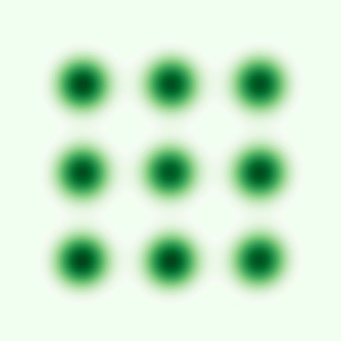
(a) Samples from true distribution $P_{X}$

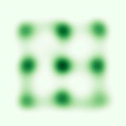
(b) Samples from generator $g_{\theta}(Z)$

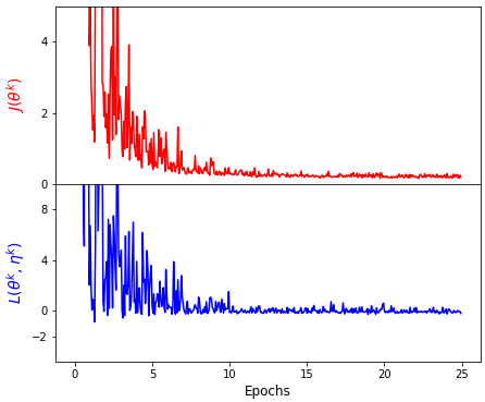
(c) Convergence of the loss functions $J$ and $L$

(d) Samples from true distribution $P_{X}$

(e) Samples from generator $g_{\theta}(Z)$

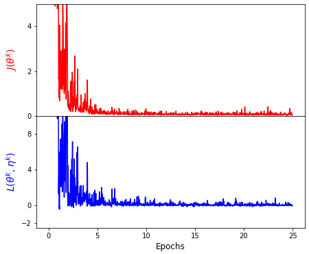
(f) Convergence of the loss functions $J$ and $L$

Figure 6: Additional experiments with mixtures of Gaussians. The code is available at https://github.com/sehyunkwon/Infinite-WGAN.

B.1 Gaussian mixture sample generation

We now provide details of the experiments for Figure 6. The code is available at https://github.com/sehyunkwon/Infinite-WGAN. The true and latent distributions are 2-dimensional, i.e., $n=2$ and $k=2$. The true distribution $P_{X}$ is a mixture of 8 Gaussians with equal weights, where the means are $(\sqrt{2}\cos\frac{m\pi}{4},\sqrt{2}\sin\frac{m\pi}{4})$ for $m=0,1,\dots,7$, and the covariance matrices are $\begin{pmatrix}0.1^{2}&0\\ 0&0.1^{2}\end{pmatrix}$. The generator feature functions are of the form $\phi_{i}(x)=\sigma_{g}(\kappa_{w}z+\kappa_{b})$ as described in (AG) for $1\leq i\leq N_{g}=5000$, where the activation function $\sigma_{g}$ is $\tanh$. Weights $\kappa_{w}$ and $\kappa_{b}$ for generator feature functions are randomly sampled (IID) from the Gaussian distribution with zero mean and variance $10^{2}$. As required in Lemma 7, we create constant hidden units by replacing two sets of $(\kappa_{w},\kappa_{b})$ with $({\bf 0}_{2\times 2},(1,0))$ and $({\bf 0}_{2\times 2},(0,1))$. The discriminator feature functions are of form $\psi_{j}(x)=\sigma(a_{j}^{\intercal}x+b_{j})$ as described in (AD) for $1\leq j\leq N_{d}=1000$ where the activation function $\sigma$ is $\tanh$. We generate $a_{j}$ and $b_{j}$ independently according to the following procedure:

• Pick $x$-intercept $\tilde{a}$ and $y$-intercept $\tilde{b}$ from $-4$ to $4$ uniformly randomly.

• Then, $\frac{x}{\tilde{a}}+\frac{y}{\tilde{b}}=1$ is the line with those intercepts.

• Pick $c$ uniformly randomly from $1$ to $10$, then set $a_{j}=(c/\tilde{a},c/\tilde{b})$ and $b_{j}=-c$.

The generator stepsize starts at $\alpha=10^{-5}$ and decays by a factor of 0.9 at every epoch. The networks are trained for 25 epochs with ($X$-sample) batch size 5000. At each iteration, 5000 latent vectors ($Z$-samples) are sampled IID from the standard Gaussian distribution for the stochastic gradient ascent step, and another 5000 latent vectors are sampled IID from the standard Gaussian distribution for the stochastic gradient descent step. The generator parameter $\theta$ is randomly initialized (IID) with the Gaussian distribution with zero mean and variance $5\times 10^{-3}$. The discriminator parameter $\gamma$ is randomly initialized (IID) with the standard normal distribution. We visualize the generated distribution using the kernel density estimation (KDE) plot.

We also perform additional experiments under distinct settings. The first additional experiment considers the true distribution $P_{X}$ that is a mixture of 9 Gaussians with equal weights. The means are $(m_{1},m_{2})$ for $m_{1}=-1,0,1$ and $m_{2}=-1,0,1$, and the covariance matrices are the same as before. We use the initial stepsize $\alpha=5\times 10^{-6}$ for the generator and $N_{g}=10,000$ for generator feature functions. The generator parameter $\theta$ is randomly initialized (IID) with the Gaussian distribution with zero mean and variance $3\times 10^{-3}$. Discriminator feature functions are generated in the same manner. Figure 6(a) shows the true distribution, and Figure 6(b) shows the generated samples. The second additional experiment considers the true distribution $P_{X}$, which is a spiral-shaped mixture of 20 Gaussians with equal weights. The means are $(\frac{m}{20}\cos\frac{2m}{20}\pi,\frac{m}{20}\sin\frac{2m}{20}\pi)$ for $m=0,1,\dots,19$, and the covariance matrices are the same as before. We use the initial stepsize $\alpha=10^{-6}$ for the generator and $N_{g}=10,000$ for generator feature functions. The generator parameter $\theta$ is randomly initialized (IID) with the Gaussian distribution with zero mean and variance $3\times 10^{-3}$. For the discriminator, feature function weights are generated by sampling $x$-intercept $\tilde{a}$ and $y$-intercept $\tilde{b}$ from $-2$ to $2$ uniformly randomly. Figure 6(d) shows the true distribution, and Figure 6(e) shows the generated samples. In both cases, the generators closely mimic the true distributions and loss functions converge to zero.

B.2 Loss landscape

In this section, we describe the experiments for Figure 5, which visualizes the loss landscape of $J(\theta)$ for the cases $N_{g}=2$ and $N_{g}=10$. We also provide additional experiments for $N_{g}=3$, $5$, and $100$. In the $N_{g}=2$ case, the landscape is highly non-convex and displays at least three non-global local minima. We observe that in Figures 8 and 8, the landscapes become better behaved, although still non-convex, as $N_{g}$ increases.

When $N_{g}>2$, the parameter space is projected down to a 2D plane spanned by two random directions, as recommended by Li et al. (2018b). The true and latent distributions are 2-dimensional, i.e., $n=2$ and $k=2$. The true distribution $P_{X}$ is a mixture of 2 Gaussians with equal weights, where the means are $(m_{1},m_{2})$ for $m_{1}=0$ and $m_{2}=\pm 2$, and the covariance matrices are $\begin{pmatrix}\sqrt{0.5^{2}}&0\\ 0&\sqrt{0.5^{2}}\end{pmatrix}$. The latent distribution is the standard Gaussian distribution. The generator feature functions are of the form $\phi_{i}(x)=\sigma_{g}(\kappa_{w}z+\kappa_{b})$ as described in (AG) for $1\leq i\leq N_{g}=2$, $3$, $5$, $10$, and $100$, where the activation function $\sigma_{g}$ is $\tanh$. Weights $\kappa_{w}$ are randomly sampled (IID) from an isotropic Gaussian and then multiplied by a scalar factor, sampled independently from the standard normal distribution. Weights $\kappa_{b}$ are randomly sampled (IID) from the Gaussian distribution with zero mean and variance $3\times 10^{-1}$. The discriminator feature functions are of the form $\psi_{j}(x)=\sigma(a_{j}^{\intercal}x+b_{j})$ as described in (AD) for $1\leq j\leq N_{d}=8$, where the activation function $\sigma$ is $\tanh$.

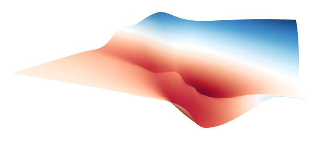
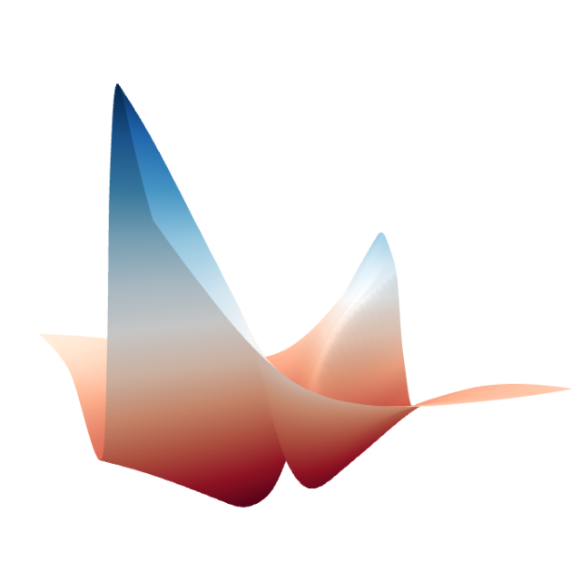
(a) $N_{g}=2$	(b) $N_{g}=3$	(c) $N_{g}=5$

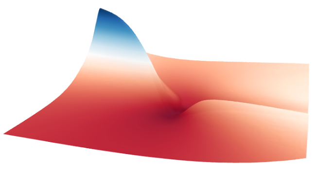
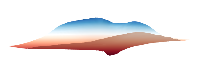
(d) $N_{g}=10$	(e) $N_{g}=100$

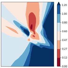
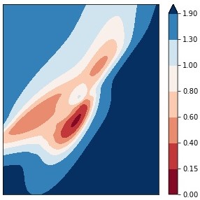
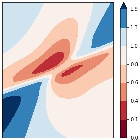
Figure 7: Loss landscapes of $J(\theta)$ for $N_{g}=2$, $3$, $5$, $10$, and $100$.

(a) $N_{g}=2$	(b) $N_{g}=3$	(c) $N_{g}=5$

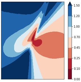
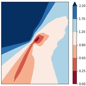
(d) $N_{g}=10$	(e) $N_{g}=100$

Figure 8: Corresponding contour plots of the landscapes of Figure 8.