On the foundations and extremal structure
of the holographic entropy cone
††thanks: DA was supported by JSPS Kakenhi Grants
16H02785,
18H05291
and
20H00579.
SHC was supported by NSF Grant PHY-1801805
and the University of California, Santa Barbara.
Abstract
The holographic entropy cone (HEC) is a polyhedral cone first introduced in the study of a class of quantum entropy inequalities. It admits a graph-theoretic description in terms of minimum cuts in weighted graphs, a characterization which naturally generalizes the cut function for complete graphs. Unfortunately, no complete facet or extreme-ray representation of the HEC is known. In this work, starting from a purely graph-theoretic perspective, we develop a theoretical and computational foundation for the HEC. The paper is self-contained, giving new proofs of known results and proving several new results as well. These are also used to develop two systematic approaches for finding the facets and extreme rays of the HEC, which we illustrate by recomputing the HEC on terminals and improving its graph description. We also report on some partial results for 6 terminals. Some interesting open problems are stated throughout.
Keywords: holographic entropy cone, polyhedral computation, cut functions, extreme rays, facets, entropy inequalities, quantum information
1 Introduction
The holographic entropy cone (HEC) has its origins in quantum physics in the work of Bao et al. [1] as described briefly in Appendix A. The HEC is a family of polyhedral cones A crucial result of their paper is a graph-theoretic characterization in terms of minimum cuts in a complete graph, which is a natural generalization of the well-studied cone of cut functions. This allows us to study the HEC without any reference to the underlying quantum physics setting. Apart from its relationship to cut functions, the HEC does not appear to be related to other known polyhedral objects. Our main focus is on the extremal structure of the HEC. At present no compact representation of either the extreme rays or the facets of is known and a complete explicit description is only known up to , see [1, 14]. The main motivation for studying the extremal structure of the HEC is the characterization of its facets, which physically correspond to entropy inequalities that strongly constrain the entanglement patterns of quantum states encoding higher-dimensional spacetimes as their quantum gravity duals in holography [1, 5] – see Appendix A for more details
This paper is structured as follows. Firstly, in Section 2 we give a formal definition of and some basic structural results that will be needed throughout the paper. These include new proofs that it is full-dimensional and polyhedral. In proving the latter result, using antichains in a lattice, we obtain a tighter bound on the size of the complete graph needed to realize all extreme rays of . We then review some basic results on the - and -representations of cones and study relating it to the cone of cut functions. In Section 3 we discuss the extreme rays of and describe some related cones that lead to methods to compute them. This gives a simple proof that the is a rational cone. It also allows us to give a description of . Following that we give a general zero-lifting result for extreme rays. In Section 4 we describe valid inequalities and facets. We begin by reviewing the proof-by-contraction method that is used for proving validity of inequalities. In the proof we again use antichains, obtaining a reduction in the complexity of the original method. This is followed by a discussion of zero-lifting of valid inequalities and facets. In Section 5 we describe integer programs that can be used to test membership in and prove non-validity of inequalities defined over it. Many of the results of the paper are combined in Section 6, which describes two methods to derive complete facet and extreme-ray descriptions of and illustrate these on computations of . There are a lot of interesting open problems related to the HEC, and some of these are stated throughout the paper and in the conclusion. Supplemental material, including input and output files, integer linear programs and C code for various functions mentioned, is available online111http://cgm.cs.mcgill.ca/~avis/doc/HEC/HEC.html.
2 Definitions and basic results
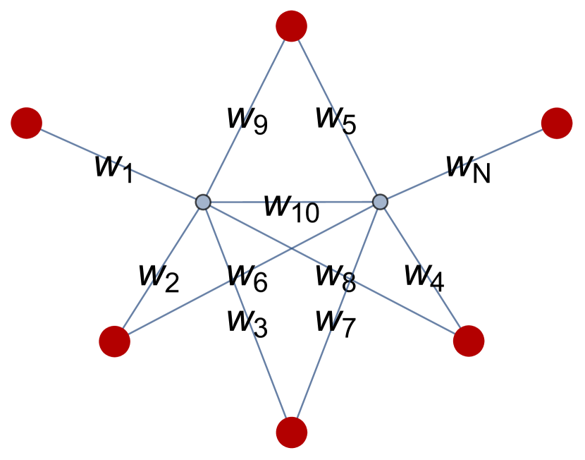
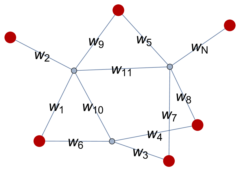
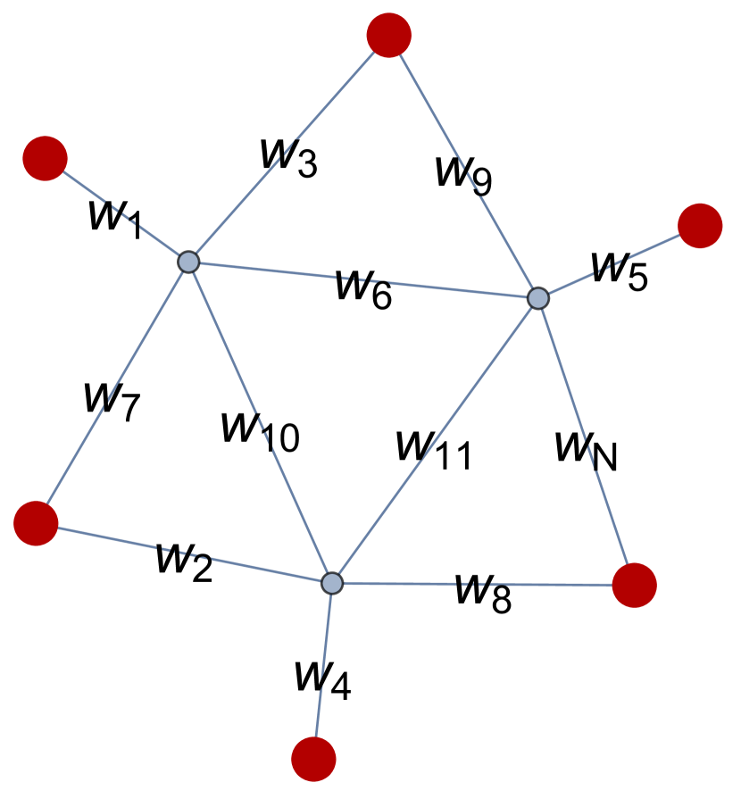
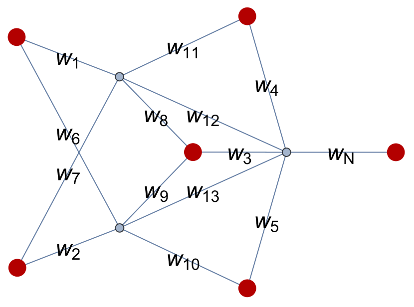
For any positive integers and , let , and let denote the undirected complete graph on the vertex set . The edge set consists of all edges between vertices for every pair . A weight map is introduced to assign a nonnegative weight to every . Any subset defines a cut as the set of all edges with and . Since both and its complement define the same cut, we will normally consider cuts where , and generally exclude the empty cut. We denote by the total weight of the cut , which is the sum of the weights of all the edges in . Letting , consider the -vector of length with entries indexed by cardinality and then lexicographically by the non-empty subsets of ,
| (2.1) |
where juxtaposition is a shorthand for the corresponding set of integers. The convex hull of the set of all vectors for a given forms a cone in . In fact, this cone is polyhedral, its facets are the subadditivity inequalities and the submodular inequalities are valid for it, as established independently by Tomizawa and Fujishige (see Section 3.6 of [11]) and Cunningham [6]. When the vector is expressed as a function of it is known as the cut function.
The HEC is a generalization of the cone defined by the cut function. We follow [1], but adapt its notation and terminology considerably. Instead of setting , we fix some integer and consider for all . In any such graph, we call the vertices terminals (cf. boundary regions in holography). The vertex is called the purifying vertex in the physics literature, but we will simply call it the sink here. Oftentimes, these will be combined into and collectively referred to as extended terminals. The other vertices, if any, are called bulk vertices (cf. the bulk spacetime).
Let be a non-empty subset of terminals, i.e. . We extend the definition of above to this new setting. For any and weight map defined on , we introduce a construct which captures all the basic properties conveyed by the RT formula in (A.1). In particular, let
| (2.2) |
where the minimization is over all . This says that takes the minimum weight over all cuts which contain precisely the terminals in and some (possibly empty) subset of the bulk vertices. Note that when we are minimizing over the single subset and the definition is equivalent to the one given earlier. In graph theory terms, is just the capacity of the minimum-weight cut or min-cut in separating from . By the duality of cuts and flows, an equivalent definition is to let be the value of the maximum flow between multiple-sources and multiple-sinks in . The max flow problems are structurally different for each but nevertheless give an efficient method of computing the .
We form an -vector from (2.2) of the form of (2.1) as we did previously, and say that realizes in or, more compactly, that is a valid pair.
Definition 1.
The holographic entropy cone on terminals is defined as
| (2.3) |
Examples of the facet defining inequalities and extreme rays of for small are given in Appendices B.1 and B.2 respectively.
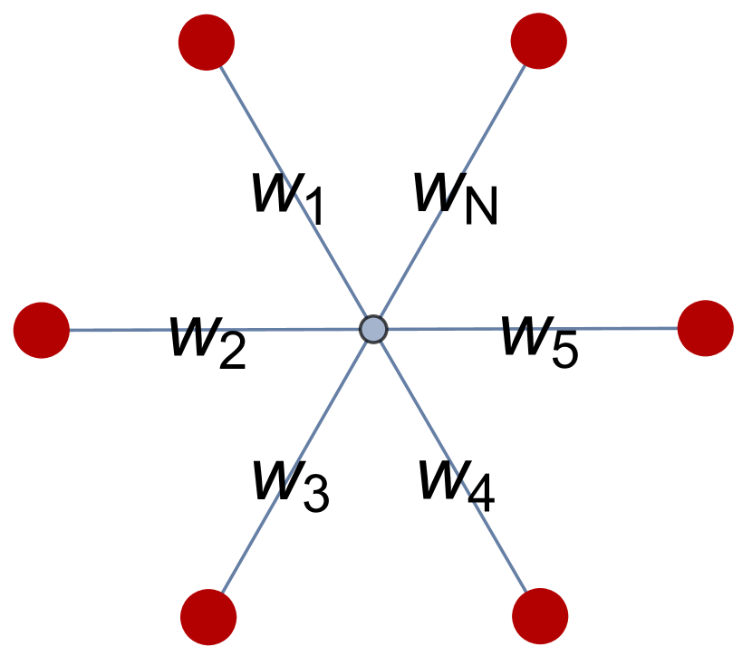
It follows from (2.2) that for any , is a valid pair for if and only if is, so is a cone. In fact it is full-dimensional. The proof employs -vectors arising from with all edges of zero weight except possibly edges for . We call these star graphs and exhibit a family of of them giving linearly independent -vectors.
Proposition 1.
is a cone of dimension .
Proof.
For each , define a weighted star graph where the nonzero edge weights are222This class of star graphs were inspired by a construction of [18].
| (2.4) |
For every , their respective -vectors can be easily seen to be given by
| (2.5) |
Using them as row vectors, we construct square matrices . For example,
| (2.6) |
where the general sketch partitions into four square matrices , , and , of size , a final column , and a final row . Note that the rows and columns have been permuted from their usual ordering for subsets of . Here, labels go first, then those of the form , and last (cf. the block forms in (2.6)). We prove by induction on that . This is immediate for . Matrix in is just reordered as described above. Since we perform the same reordering for rows as for columns the determinant sign is unchanged, so by the induction hypothesis . As the rows of and are indexed by , we have . Additionally, one easily verifies that in the first entries are and the rest are . Row has the same pattern.
We now make a comparison between entries in column of and column of . Consider the diagonal elements of each. For row , in we have column and so . In the column label is also and since we have and so . Hence the diagonals are identical. Now consider the elements below them. For each row index contains but none of its column indices do, so . In the same applies but the intersection now includes , so the corresponding entry is always bigger by one. These facts are illustrated by the coloured entries in .
We now subtract the first columns of from the next columns, then subtract from each of these columns also, obtaining
| (2.7) |
Here and respectively denote all- or all- matrices of suitable size. In the resulting , notice that is an upper triangular matrix with all diagonal elements equal to . Recalling that , we have , as desired. ∎
We will show in the following sections that is also convex, polyhedral and rational. One important basic property the -vectors do not possess is monotonicity, as can be seen by examples in Appendix B.2.
2.1 Polyhedrality of the HEC
The polyhedrality of the HEC was established by Bao et al. [1]. We give a proof of this crucial result here following similar lines to the original proof but obtain a tighter result due to our use of antichains. In general, there may be more than one min-cut for each achieving the minimum in (2.2). Among these, let denote one which is minimal under set inclusion. We call a minimal min-cut for and have . The following basic theorem shows that these are unique and builds on results from Lemma of [20], and Theorems and of [2].
Theorem 1.
For positive integers , consider a weighted complete graph with terminal set . Let and be minimal min-cuts for . Then:
-
(a)
Each has a unique minimal min-cut .
-
(b)
.
-
(c)
.
-
(d)
If , then all minimal min-cuts can be represented in a weighted .
Proof.
-
(a)
Suppose and are minimal min-cuts for . Submodularity of the cut function gives
(2.8) Clearly, and are cuts for . Since and are additionally min-cuts,
(2.9) thereby turning all inequalities above into equations. Hence is a min-cut and, as an intersection of minimal ones, minimal as well. It must thus be the case that .
-
(b)
First assume that . Since and are cuts for and respectively, we have and . As , we have . Hence .
Now assume that . Again, as min-cuts, and , and therefore and . This means and are respectively cuts for and . Then submodularity and minimality, applied to and as in the proof of (a) above, imply , which proves the claim.
-
(c)
By the definitions, implies that .
For the converse, suppose that and that there exists a vertex . Let and be the total weight of edges from to, respectively, , and . Since is a min-cut, , for otherwise we could remove from without increasing the weight of the cut. Similarly, by considering , we have . As edge weights are nonnegative, this gives the desired contradiction.
-
(d)
Firstly, we renumber the vertices in so that vertices cover all of the vertices in the union of the . In we will let take the role of the sink and adjust weights as follows. We leave the edge weights unchanged between edges with both endpoints in . For we give edge the weight corresponding to the sum of the weights of all edges with . It is easy to verify that the weights of the min-cuts are preserved: if a smaller weight cut for a terminal set existed in , then it could be reproduced in the original , a contradiction.
∎
Unfortunately, part (b) above does not generalize to the intersection of three or more sets. A simple example is given by the star graph with unit weights for the terminal edges and zero for the sink edge. In particular, the intersection of the three pairs of terminals is of course empty, but the intersection of their minimal min-cuts is not as it contains the bulk vertex.
Each -vector is realized in for some , and we are interested in the smallest such . More generally, for a given , is there a smallest integer such that all -vectors on can be realized in ? The answer is yes and this was proved by Bao et al. [1] (Lemma ) who obtained . A tighter bound can be obtained from Theorem 1 as follows.
Let denote the Boolean lattice of all subsets of ordered under inclusion. A family of subsets of , , is an upper set if for each and that contains we have . For , we call pairwise intersecting if each pair of its constituent subsets has a non-empty intersection. If is the empty set or consists of a singleton, we consider to be pairwise intersecting. An antichain is a collection of subsets of which are pairwise incomparable, i.e. none of them is contained in any of the others. Notice that the minimal elements of any upper set form an antichain and that is pairwise intersecting if and only if its upper set is. Let denote the number of pairwise interesecting antichains in . We can use this value to bound as follows:
Corollary 1.
For , every -vector for terminals can be realized in , where
| (2.10) |
Proof.
We first sketch the argument in [1] for their upper bound on . Suppose a given -vector on terminals can be realized in a weighted , for some given . For , partitions the vertex set of into two subsets. If we intersect these by , for some , we get subsets, some possibly empty. After repeating for all non-empty subsets of we obtain a partition of into subsets, many of which may be empty. However, in each of the non-empty subsets, the vertices of may be merged into a single vertex by combining edge weights (cf. Theorem 1(d)). This new complete graph has at most vertices and realizes the same min-cut weights as before, giving their result.
To improve this bound we use Theorem 1. For a set , denote its complement by . Any atom in the partition just described is formed by splitting the non-empty subsets of into two disjoint, spanning families and , and taking the intersection
| (2.11) |
Suppose this intersection is non-empty. Theorem 1(c) implies that is pairwise intersecting, for otherwise the left intersection in (2.11) is empty. In particular, this implies that both a subset and its complement cannot be in . In addition, one can show that must either be empty or an upper set in as follows. If , then (2.11) is in fact never empty because it will always contain vertex . As for , consider two subsets and suppose is non-empty. We have by Theorem 1(b) that and so , implying that if , then (2.11) is empty. As a result, either or must be a pairwise intersecting upper set in , with containing all other non-empty subsets of .
Because empty atoms from (2.11) do not contribute to min-cut weights, it follows that when considering -vectors we need only be concerned with pairwise intersecting upper sets in and . As described above, the upper sets can be equivalently enumerated as the number of pairwise intersecting antichains in . Since counts their number, we conclude that all -vectors with terminals can be realized in . ∎
We have the following reasonably tight asymptotic bounds on . Let be the total number of antichains in . Then,
| (2.12) |
The asymptotic upper bound on is due to Kleitman and Markowsky [19]. The lower bound can be obtained by considering all subsets of of size . Each pair of such subsets intersects and none can properly contain another. So any collection of these subsets forms an intersecting antichain. While we do not know of tighter asymptotic bounds for , exact values are known [4]333 is entry in Proposition of [4]. for :
| (2.13) |
However, it seems that is a very poor upper bound on . For example, data for shows that – see Section 5 for more details.
Problem 1.
Find tighter bounds on . In particular, does admit an upper bound that is polynomial in ?
Definition 1 suggests the following family of cones, which are useful in proving the polyhedrality of . For any pair of integers and such that , consider
| (2.14) |
This is a generalization of the cone defined by the cut functions, which corresponds to the specific case . Without the convex hull operator in (2.14), would not be convex in general, as shown by example in Appendix C. An important property of is that it is naturally invariant under the action of the symmetric group which permutes the elements of the set . In fact, enjoys a larger symmetry group: it is symmetric under permutations of vertices in the extended terminal set . The permutations of under yield -vectors (2.1) which are related by the simple fact that . Similarly, in an undirected graph any min-cut is insensitive to the exchange of its sources and sinks. When talking about symmetries under , it is thus convenient to identify .
It is easy to see that in general , since an additional bulk vertex can always be added to with all edges containing it of weight zero. We are now able to prove that is a convex polyhedral cone. Our bound is tighter than the original proof given in [1] due to our use of antichains.
Corollary 2.
For any , is a convex, polyhedral cone given by .
Proof.
Firstly, suppose . Then for some and weight set the pair satisfies (2.2) and so . Conversely, suppose is in the convex hull of extreme rays of . Each of these rays can be realized in a weighted for some . For a specific conical combination of extreme rays giving , consider the graph obtained by identifying all of their associated graphs at their terminal vertices, each with its edge weights multiplied by the coefficient in the associated conical combination. This graph clearly still realizes ,444This is basically the statement that any flow network problem with multiple source/sink vertices can be equivalently reformulated in terms of a single supersource/supersink vertex connected to each of the sources/sinks with edges of infinite capacity. In our case, however, it is preferable to simply merge together terminals of the same type into a single “superterminal”, rather than having unnecessary infinite-weight edges. and can be thought of as a for some large but finite with many zero-weight edges omitted. However, the bound on in Corollary 1 guarantees that by merging vertices this graph can be reduced to one with , thus proving convexity. ∎
Of course, inherits the symmetry discussed above. As a result, when considering the extremal structure of , we will only specify single representatives of symmetry orbits under .
Almost nothing is known about the complexity of computational problems related to .
Problem 2.
Given a vector , what is the complexity of deciding if ? What is the complexity of deciding whether is satisfied for all ?
2.2 Representations of the HEC
A basic result of polyhedral geometry is that any polyhedral cone can be represented by a non-redundant set of facet-defining inequalities, which we can write as for a suitably dimensioned matrix and variables , and is called an -representation. One can also represent by a non-redundant list of its extreme rays, such that , which is called a -representation. Both representations are unique up to row scaling. In this paper we are concerned with computing the - and -representations of . Normally, for cones (or polyhedra) arising in discrete optimization, we have available one or the other of the representations. However, this is not the case for . To proceed we will initially try to find both valid inequalities for , which are those satisfied by all rays in , and to find feasible rays of . A set of valid inequalities forms an outer approximation of and a set of valid rays forms an inner approximation. The following well known basic result shows when such sets respectively constitute an - and -representation (see, e.g., Schrijver [25]).
Proposition 2.
For a given polyhedral cone , let be a non-redundant set of valid inequalities and let be a non-redundant set of feasible rays. Then:
-
(a)
An extreme ray of is an extreme ray of if it is feasible for .
-
(b)
A facet of is a facet of if it is valid for .
-
(c)
is precisely the set of extreme rays of if and only if they respectively constitute - and -representations of .
Parts (a) and (b) lead to a kind of bootstrapping process which terminates once (c) can be applied. This is described in detail in Section 6, but to illustrate we now look at some small values of .
For , the -vectors are the nonnegative real numbers. There is one facet and one extreme ray with , and Proposition 2(c) is readily verified. Notice that this simple extreme ray can be represented in with the single edge having weight . More generally, any where two distinct singletons share a unit-weight edge and all other weights are zero will be called an Bell pair. The -vector of such a Bell pair has nonzero if and only if either or , but not both.
For we have and a valid inequality . This follows since the union of cuts for two terminals is always a cut for the union of the two terminals . Hence the latter’s min-cut cannot have larger weight than the sum of the weights of the two other cuts. The full orbit of contains and . All three are related by the symmetry of permutations of and the identification of for all . In the context of information theory, the first one is known as subadditivity (SA), while the latter two are called the Araki-Lieb inequalities.
Subadditivity generalizes to a valid inequality for any disjoint, non-empty subsets of terminals with to give
| (2.15) |
We exclude since in this case SA reduces to nonnegativity. Every inequality in the enlarged symmetry orbit of (2.15) clearly remains valid. For any disjoint subsets of terminals , those of Araki-Lieb type take the form . The qualitative difference between SA and Araki-Lieb is that in the former the disjoint subsets do not contain the sink, whereas in the latter one of them does, and whenever one identifies . For future convenience, we introduce
| (2.16) |
known as the mutual information in the physics community. This way, SA corresponds to the nonnegativity of the mutual information .
Proceeding as suggested by Proposition 2(a), we can compute the extreme rays arising from (2.15) by the action of , together with the nonnegativity inequalities (in fact, the latter are redundant and can be ignored). Doing so we obtain extreme rays related by symmetry, of which one is . This can be represented in by a Bell pair. Obviously, this can also be obtained from the Bell pair for in by adding a new vertex with all edge weights to it zero. This is a process called a zero-lifting of extreme rays and which we discuss in detail in Section 3.2. So if we let be the set of output rays and be the SA inequalities we are again done by Proposition 2(c).
3 Extreme rays
Since we do not have an -representation of we have no direct way to compute its extreme rays. In this section we introduce a lifting of to a cone for which we can explicitly write an -representation. Computing the extreme rays of this cone and then making a projection allows us to compute a superset of the extreme rays of . This construct provides the first systematic procedure for obtaining , thus significantly improving on the random searches used so far in building the HEC [1, 14]. We also describe a zero-lifting operation, which allows known extreme rays for -vectors defined on terminals to generate extreme rays for those defined on terminals.
3.1 A lifting of the HEC
For integers and such that , consider the following system of inequalities whose variables are the -vector entries and the edge weights of :
| (3.1a) | |||||
| (3.1b) | |||||
Note that for each cut there is precisely one such that . Since we are excluding the case , this implies that (3.1a) contains inequalities. There are an additional nonnegative inequalities from (3.1b). Since each is just a sum of weights for every , together with the variables , there are a total of variables involved in (3.1). Let denote a vector of length representing these variables.
Definition 2.
The cone denotes the set of all satisfying (3.1).
Since is given explicitly by (3.1), it is a rational cone. Note that the variables in are not bounded from below. One could add the inequalities but this greatly increases the complexity of the cone, as explained below.
The cones and cannot be directly compared, since they are defined in different dimensional spaces. So we first define a lifting of by
| (3.2) |
which is by definition a subset of and whose projection onto the coordinates is . We similarly define . An example in Appendix C shows that is in general non-convex without the convex hull operator. It is easy to see that contains trivial extreme rays. These are formed by setting either one or one , and all other variables zero.
Each extreme ray of is the projection of a non-trivial extreme ray of , as we now show:
Theorem 2.
-
(a)
If is a non-trivial extreme ray of , then .
-
(b)
If is an extreme ray of , then there is a weight vector such that is a non-trivial extreme ray of .
Proof.
-
(a)
Suppose that defines a non-trivial extreme ray of . Then there must be a set of at least inequalities in (3.1) satisfied as equations whose solutions have the form , with . Each must be present in at least one of these equations or else it could be increased independently of the others and the resulting vector would still be a solution of the equations but not of that form. This in turn implies that satisfies (2.2) for the given weight function . Hence .
-
(b)
Suppose is an extreme ray of . Since satisfies (2.2), all of its values are nonnegative and there must exist a corresponding weight assignment . We now define a face of by intersecting it with the hyperplanes
(3.3a) (3.3b) Each appears in at least one equation. is defined by a set of extreme rays of but none of these can be a trivial ray of the type since . There may be a trivial extreme ray of the type as long as and the edge does not appear in any of the cuts in the system of hyperplanes. Suppose that there are of these and write each of them as . Also, denote the non-trivial extreme rays of that lie on by , with . From part (a) above, we have that for all . Writing as a conical combination of the extreme rays that define ,
(3.4) we deduce that . Since is an extreme ray of it follows that for all for which . For each such , is a non-trivial extreme ray of .
∎
It was initially hoped that non-trivial extreme rays of would project to extreme rays of , but an example in Appendix C show that this is not the case. Also, a direct projection of onto its coordinates does not give . For any given values of the coordinates, a feasible solution to inequalities (3.1) can be obtained by choosing any suitably large coordinates. Hence the projection is simply the whole space . Nevertheless, we do obtain a method in principle for obtaining a complete description of :
Corollary 3.
A -description of can be obtained by computing the extreme rays of , projecting to the coordinates, and removing both the trivial and the redundant rays.
Proof.
This important new result allows for a constructive derivation of (for which no explicit representation is known) starting from (for which a -representation is straightforward to write down). Since is a rational cone, as remarked earlier, it follows that is also. This fact, proven in Proposition of [1] by a different technique, means extreme rays and facets always admit integral representations. With our current upper bound on the computation is impractical except for small values of . It does not help here to include the extra inequalities because this introduces a large number of new extreme rays of which are not valid pairs. For example, while has extreme rays of which are trivial, adding nonnegativity yields extreme rays, all but of which do not yield valid pairs. A computationally lighter method to test whether a given -vector is realizable is as follows:
Theorem 3.
If , then there is a weight vector such that is a vertex of the polyhedron defined as the intersection of and the hyperplanes .555The converse of this is false, as generally has many vertices for which does not realize .
Proof.
First we suppose that . Then there exists a weight vector for that realizes . By construction is contained in and so is non-empty. Since all components of in are fixed, is a possibly unbounded polyhedron with vertices of the form and possibly additional extreme rays of the form for edges that do not appear in any minimum-weight cut obeying and . We can write
| (3.5) |
for a set of vertices of . For a cut in , let and denote its weight using and , respectively. Since is a realization of , for each there exists a min-cut such that . Now, by (3.5) and the linearity of the cut weight function,
| (3.6) |
Hence by (3.1a) we must also have for all . It follows that each is a vertex of representing . ∎
We now show how these theorems can help in determining the extremal structure of . For example, we can compute the extreme rays of , project onto the -coordinates, delete the trivial rays and remove redundancy, getting a -representation of . It contains extreme rays in dimensions. The -representation of is easy to compute and contains facets. One facet is new and the other are SA inequalities:
| (3.7) |
where is the sink and we recall that . Earlier we saw that for there is one SA orbit of facets: , , and . Although the first one remains a facet of the form of (3.7) for , the other two do not, which may seem surprising. We return to this in Section 4.2 when discussing the lifting of facets (see Proposition 8).
3.2 Zero-lifting extreme rays
Extreme rays for remain extremal for larger values of as the following result describes:
Proposition 3.
If is an extreme ray of , then, by adding suitably many new weight coordinates set to zero, it is an extreme ray of for every . Hence is a projection of .
Proof.
Let define an extreme ray of and consider the base graph . We extend the weight vector by adding new coordinates to get a vector of length . We set for and for . All edges containing vertex receive weight zero in , and vertex is the new sink. Since is now a bulk vertex, it may participate in a cut , but since , it will never change its total weight. Hence . Since defines an extreme ray of we can choose inequalities in (3.1) which, when satisfied as equations, have solutions in of the form with . To these equations we add the equations . The resulting system has solutions in of the form with , and the extremality of the ray defined by follows. ∎
Extreme rays can also be preserved under the addition of new terminal vertices as follows. Given , we define its zero-lift as the vector , where has dimension and has dimension , by
| (3.8a) | ||||
| (3.8b) | ||||
Similarly, above defines the zero-lift of the given . A vector that satisfies an inequality as an equation is called a root of that inequality.
Proposition 4.
If is an extreme ray of , then its zero-lift is an extreme ray of .
Proof.
Let define an extreme ray of . For each choose an inequality from (3.1a) for which it is a root. These are linearly independent inequalities since the coordinates define minus the identity matrix. To these inequalities add all those from (3.1b) for which is a root. Since is an extreme ray we have a linearly independent set of such inequalities. Call this system . We now add terminal and define and as above. It is easy to verify that . Note has more dimensions than and we will augment by this many linearly independent inequalities. Firstly, for each the inequality previously chosen will also be satisfied as an equation when is replaced by . This gives an additional inequalities which are linearly independent from the others in since the new variables again form minus the identity matrix. To these we add equations for and the equation . This gives the required number of tight linearly independent constraints. By construction, their solution is with , which proves that defines an extreme ray of . ∎
The following result, though not unexpected, is proved here for the first time:
Proposition 5.
If is an extreme ray of , then its zero-lift is an extreme ray of . Hence is a projection of .
Proof.
If is an extreme ray of , then it is a root of a linearly independent set of of its facet inequalities. Clearly is also a root of these inequalities. Additionally, is a root of the following instances of SA,
| (3.9) |
for all , and also obeys . This gives more equations which are linearly independent and are also independent of the former because they independently involve the new, distinct variables for every . Since satisfies independent valid inequalities as equations, it is an extreme ray of by Proposition 2(a). ∎
To illustrate the use of the results in this subsection we consider the case . If we compute and remove the trivial rays we have extreme rays. When we project onto the coordinates and remove redundancy, there remain extreme rays. Only of these are new, whereas the other come from zero-lifts of the two extreme-ray classes that define . The convex hull of this set is bounded by facets that are examples of what is called zero-lifting from the two facet classes for . We will define this process and prove that it preserves validity and facets in Section 4.2. By this result and Proposition 2(c) we have obtained the - and -representations of .
4 Valid inequalities and facets
As remarked in Section 2, there is no general explicit -representation known for , although it can in principle be computed by using the method of Corollary 3 and then converting the resulting -representation into an -representation. In Section 5 we give an integer linear program (ILP) for testing whether an inequality is valid over or not. However, to prove validity would require solving an ILP whose size depends on and so is impractical with current bounds. The main result of this section is a tractable method known as proof by contraction to prove inequalities valid for . By exhibiting the required number of extreme rays it is then possible to prove they are facets.
A general inequality over is specified by a vector . Let be the subset of terminals appearing in it, i.e. if and only if for some . If , one can turn it into an inequality over by relabelling terminals , if necessary. We say that an inequality over is in canonical form if , and write it canonically as
| (4.1) |
where and are respectively the number of positive and negative entries in the vector , and for all and , the coefficients and the sets are distinct and non-empty. Because is a rational cone, the normalization of (4.1) of any inequality of interest is always set such that all coefficients are together coprime integers.
At the end of Section 2.2 we discussed the cases . Recall that is -dimensional and corresponds to a nonnegative half-line. Its only facet is , which trivially follows from nonnegativity of the weights in (2.14). For , we saw that the resulting -dimensional cone is a simplex bounded by the facets in the symmetry orbit of the SA inequality (2.15). We discussed at the end of Sections 3.1 and 3.2. Apart from the SA orbit, containing facet inequalities, an additional inequality was discovered to bound [12]:
| (4.2) |
This is known in physics as the monogamy of mutual information (MMI) due to its rewriting using (2.16) as . Since one can write submodularity as , by nonnegativity of one sees that MMI is a strictly stronger inequality. The proof of the validity of (4.2) will be presented in Section 4.1 (see Table 1) as an example of a general combinatorial proof method for valid inequalities of . This will show that has facets and so is also a simplex. As we saw at the end of Section 3.2, no new inequalities arise for . However, for note that MMI acquires a more general form which we show is valid for : for disjoint non-empty subsets ,
| (4.3) |
which is valid for , as we show in Section 4.2.
4.1 Proof by contraction
We now describe the proof-by-contraction method for proving validity of inequalities for . Although our description is complete, we refer the reader to [1] and [3] for more details on its derivation. By making use of antichains, as in Corollary 1, we obtain a stronger result than previous ones. Our discussion will be exemplified with MMI as given in (4.2).
To set the stage, let denote the (vertices of) the unit -cube and refer to as a bitstring. At times, it will also be useful to think of as an -ary Boolean domain. Given some vector of positive entries , we can turn into a metric space with distance function by endowing it with a weighted Hamming norm via
| (4.4) |
Consider now a candidate inequality in canonical form over , written as in (4.1). Encode each side of it into occurrence vectors, and for , with entries
| (4.5) |
where is a Boolean indicator function, i.e. it yields or depending on whether its argument is true or false, respectively. Clearly, the occurrence vectors for are all- vectors. For inequality (4.2), the occurrence vectors are the following bitstrings:
| (4.6) | |||||
Bitstrings are a bookkeeping device for partitioning the vertex set of into specific disjoint subsets suitable for studying a given candidate inequality. In particular, consider the minimal min-cuts for associated to every term on the left-hand side of (4.1). Each of the different bitstrings indexes a disjoint vertex subset defined by
| (4.7) |
The attentive reader will notice that these sets would be precisely the atoms introduced in (2.11) when proving Corollary 1 if one were to iterate the intersection over all possible non-empty subsets of . In the current discussion, one need only consider the pertinent subsets involved in the left-hand side of (4.1). The resulting sets are again disjoint by construction, i.e. unless . The converse is certainly not true though, as expected from Corollary 1. In particular, will be empty whenever the family of sets is not a pairwise intersecting upper set in . The relation between this statement and the one in Corollary 1 that refers to upper sets in is better understood in terms of their associated antichains. Namely, will be empty whenever the minimal elements in are not a pairwise intersecting antichain in , which holds if and only if the same is true in . In other words, there is a non-trivial precisely for every pairwise intersecting antichain in that is also so in , and thus the number of relevant bitstrings will be considerably smaller than .
The discussion above motivates introducing the subset of all bitstrings such that is a pairwise intersecting antichain in . Crucially, these suffice to characterize the minimal min-cuts for in any , in the sense that these are all reconstructible via
| (4.8) |
where the union here, and in all that follows next, runs over all bitstrings subject to the given conditions. Furthermore, one can use these vertex sets to construct (not necessarily minimum) cuts for any subset of terminals . To see this, let be any one of the terminals involved in the subsets . We want to find which of the sets the vertex lands on. Since if and only if by the definition of a cut for , it follows that if and only if precisely when and otherwise. In other words, the bitstring we are after is precisely the occurrence vector defined in (4.5), and we thus have .
Lemma 1.
Let be an -ary Boolean function. Given some collection of terminal subsets and the partitioning of defined in (4.7), construct the vertex set
| (4.9) |
Then, for any subset of terminals , we have
| (4.10) |
Proof.
A trivial rephrasing of is that, for , one has if and only if . Since for every and all are disjoint, it follows that if and only if . Finally, since by construction if and only if , the desired result is obtained. ∎
The min-cut edges can also be conveniently organized in terms of bitstrings via
| (4.11) |
Because the vertex sets are disjoint, so are the edge sets for any distinct pair of bitstrings . This leads to the following useful result for :
Lemma 2.
The edges of a min-cut for some and their total weight are, respectively,
| (4.12) |
where the index sets are unordered pairs of bitstrings .
Proof.
By definition, an edge if and only if and . Using (4.8), one can write and, similarly, . Hence is contained in if and only if and differ in their bit . It follows that can be constructed by joining all edge sets with bitstrings such that , thereby proving the first equation in (4.12). Furthermore, since all are disjoint for distinct pairs of bitstrings, the total weight of their union reduces to the sum over the total weights of every involved, which is precisely what the second equation computes. ∎
Given two metric spaces and , we call a - contraction map if
| (4.13) |
The general proof method can now be stated:
Theorem 4.
Proof.
Associate a cut to each subsystem that appears on the right-hand side of (4.1) by using the map to pick which sets to include in the definition of as follows:
| (4.15) |
That this indeed obeys the cut condition is guaranteed by Lemma 1 and the fact that is required to respect occurrence vectors, i.e. for every .
| (4.16) |
Similarly, for the cuts one has
| (4.17) |
Therefore, by hypothesis, the contraction property of implies
| (4.18) |
Because every set is a cut for each appearing on the right-hand side of (4.1), by minimality for every . Hence the right-hand side of (4.18) is no smaller than that of (4.1). Finally, since their respective left-hand sides are equal, validity of (4.1) follows. ∎
This theorem was proved in [1] (Theorem ) in a somewhat weaker form. Whereas the domain of their contraction map is , enumerating all subsets of , we reduce this to , enumerating only the pairwise intersecting antichains in (cf. Corollary 1). This leads to a reduction of the worst-case complexity of the search space.
As an example, a contraction map which proves validity of (4.2) is shown in Table 1.666In fact, this contraction map which proves (4.2) is unique. This is generically not the case for larger- facets, for which there usually exists many contraction maps compatible with the requirements of Theorem 4. One easily checks that occurrence vectors are respected, e.g. for we have , which matches (4.6). Iterating through every pair of rows, one can also check that the contraction property holds. Here the vectors defining the distance function are and for left and right, respectively. For instance, occurrence vectors and in the domain give , while their images . Notice that the map need not be injective nor surjective.
| 0 | 0 | 0 | 0 | 0 | 0 | 0 | |
|---|---|---|---|---|---|---|---|
| 0 | 0 | 1 | 0 | 0 | 0 | 1 | |
| 0 | 1 | 0 | 0 | 0 | 0 | 1 | |
| 0 | 1 | 1 | 0 | 0 | 1 | 1 | |
| 1 | 0 | 0 | 0 | 0 | 0 | 1 | |
| 1 | 0 | 1 | 0 | 1 | 0 | 1 | |
| 1 | 1 | 0 | 1 | 0 | 0 | 1 | |
| 1 | 1 | 1 | 0 | 0 | 0 | 1 |
The proof of Theorem 4 is constructive and, as shown in [1], leads to an algorithm for finding a contraction map or showing none exists. The enumeration of all contraction maps is prohibitively expensive in all but very small cases. However, the authors developed a greedy technique for partial search which is successful in finding a map, when one exists. Indeed, we have found this method very powerful in proving new inequalities valid for . For proving an inequality is invalid, the previously-mentioned ILP approach, which will be presented in Section 5, is also very effective.
Theorem 4 provides a robust sufficient condition for an inequality to be valid, but it is not a necessary one. For example, even after exhausting all of the possibilities given by the theorem, it was not able to prove the validity of this inequality over :
| (4.19) | ||||
However, this inequality can be proved valid by expanding the codomain of by replacing coefficients greater than one on the right-hand side by a sum of terms with unit coefficients. For instance, a term like gets replaced by , with the obvious generalization applied to larger coefficients. Theorem 4 still applies and this time the desired contraction map does exist, thereby proving validity of (4.19) By expanding the right-hand side there are more possible images for the contraction map, while the number of contraction conditions remains fixed. This may explain why this approach worked well here and in other cases we have tried for larger .
This mild generalization of the proof technique of Theorem 4 has been remarkably successful in proving inequalities for , which motivates the following problem:
4.2 Zero-lifting of valid inequalities and facets
Given an inequality over , let be the subset of terminals appearing in it. Then consider a family of disjoint, non-empty subsets (not necessarily spanning). The zero-lifting of the inequality given by this family is obtained by replacing each singleton in every in by its corresponding . For example, the zero-lifting of from to corresponding to and yields . The zero-lift where for every is called the trivial zero-lift.
Proposition 6.
If an inequality is valid for , then any zero-lift is valid for .
Proof.
Assume is valid for . Proceed by contradiction by supposing has a zero-lift such that for some . Such must be realized by some weight map applied to for some . In this , contract each terminal set to the vertex in with the minimum label, combining parallel edges and summing their weights into a single edge, and deleting any loops. Let be the realized -vector in the new graph. We have , the desired contradiction. ∎
Before discussing lifting facets we need to recall some terminology from Proposition 1, in particular the weighted star graphs and the construction of matrix in (2.6). We will make frequent use of the square matrix of size , defined by
| (4.20) |
and use the notation to refer to row of . An inequality in is called balanced if for all . By definition, balance is invariant under any permutation of terminals , but need not be so under permutations of the extended terminals . For instance, is balanced but is not. Balance is equivalent to a seemingly stronger condition:
Lemma 3.
An inequality in is balanced if and only if .
Proof.
Obviously, implies balance. For the converse, writing out row of ,
| (4.21) |
where (cf. (4.5)) and we used . So by balance. ∎
What follows is a new result which relates the trivial zero-lifting of facets to the notion of balance:
Proposition 7.
If is a balanced facet of , then its trivial zero-lift is a balanced facet of .
Proof.
Suppose is a balanced facet of . Then it is a valid inequality of by Proposition 6. We adopt the notation of Proposition 1 and build a matrix with the structure in (2.7), except it will now have only rows. Let consist of linearly independent roots of as rows, so that the first rows of become precisely their zero-lifts. The trivial zero-lift has for every , so these are all roots of as well. Since is balanced we have by Lemma 3. So the corresponding rows of are roots of too. The final row is also and so contains roots of . Performing the same column operations as in Proposition 1, the resulting block matrix (cf. ) shows that has maximal rank . Since , the lifted facet is also balanced. ∎
The following proposition clarifies the situation for subadditive inequalities, which include the non-balanced Araki-Lieb inequalities in their orbits:
Proposition 8.
For all , a zero-lift of a subadditive inequality (2.15) gives a facet if and only if, using the symmetry , it can be put in the singleton SA form
| (4.22) |
Proof.
Since singleton SA is a balanced facet of , so is for by Proposition 7, as it can be obtained by iterating trivial zero-lifts and making a permutation at the end.
Apart from nonnegativity and the Araki-Lieb inequality associated to (4.22), all known facets of are balanced. While balance is sufficient for trivial zero-lifts to preserve facets, a stronger condition is needed for general zero-lifts. A balanced inequality is superbalanced if every inequality in its symmetry orbit under permutations of is balanced [18, 13]. Since balance is invariant under permutations of , it is in fact only necessary to check if exchanges of every with yield balanced inequalities. Orbits of superbalanced inequalities are referred to as superbalanced. For example, SA in (2.15) for is balanced but not superbalanced and MMI in (4.2) is superbalanced. According to results stated in [13], besides the singleton SA orbit, every orbit of facets of for is superbalanced.
We can now generalize Proposition 7 to arbitrary zero-lifts. For an inequality in , let
| (4.23) |
Lemma 4.
An inequality in is superbalanced if and only if for every with .
Proof.
That for all is just the definition of balance, which is an invariant property under permutations of . Permutations of also allow for reflections for each . Using , the -vector entries after reflection are related to the before reflection by and for . For example, for gives . The coefficients in behave accordingly. Under a reflection, (4.23) gives , while for one gets
| (4.24) |
The first sum is over all such that but , so it differs from precisely by . Similarly for the second sum exchanging , so
| (4.25) |
After the exchange , is balanced if and only if for all . Therefore is superbalanced if and only if for all . Applied to (4.25), this means is superbalanced if and only if for all . ∎
We now show that any zero-lift of a superbalanced facet can actually be built solely out of trivial zero-lifts combined with permutations of the extended terminals, both of which preserve facets. Superbalance is needed for such permutations to preserve balance and thus keep Proposition 7 applicable. It is also important in what follows that, as is clear from Lemma 4 and the form of (4.23), balance and superbalance are properties which are shared by inequalities related by trivial zero-lifts. We first observe that the trivial zero-lift from to can be thought of as treating the new terminal as a duplication of the sink (since the sink does not appear anywhere in , neither does in ). But by the symmetry of under permutations of , we could analogously consider letting duplicate any other terminal. Let us call such a generalization of a trivial zero-lift where any one extended terminal becomes a doubleton and the rest remain singletons a simple zero-lift. We obtain the following novel result:
Theorem 5.
If is a superbalanced facet of , then any zero-lift is a superbalanced facet of .
Proof.
If is a facet inequality over involving a subset of terminals with , then put it in canonical form as an inequality over . Iterating Proposition 5, note that is a projection of . Since is in canonical form, its coefficients are not changed in projecting it to . A standard result of polyhedral theory is that facets project to facets, so is a superbalanced facet of .
Starting from , one can get to as follows. If the original zero-lift had , perform simple zero-lifts appending terminals to , and repeat for every . If less than steps were required, reach all the way to via trivial zero-lifts. At that point, a suitable permutation of yields .
We now show that every simple zero-lift used above can in fact be built solely out of permutations and trivial zero-lifts. In particular, the simple zero-lift involving is equivalently accomplished by exchanging , performing a trivial zero-lift, and then exchanging the new sink back with . If the original inequality is superbalanced, the trivial zero-lift in this process is applied to a balanced inequality. Using Proposition 7, one ends up with a facet if one started with a facet. Furthermore, the latter is superbalanced if the former is. Hence one can go from to via superbalance- and facet-preserving steps. ∎
5 Integer programs for testing realizability and validity
This section describes novel methods for checking if an -vector is realizable (and if so finding a graph realization), and for checking if a given inequality is valid. A direct test of the realizability of an -vector in can be performed by a feasibility test of a mixed integer linear program (ILP). Similarly, an inequality can be tested to see if it is valid for all -vectors that can be realized in . As noted earlier, the polyhedral approach described so far does not force the minimum in (2.2) to be realized by one of the inequalities (3.1a). However, using binary variables this can be achieved and the feasibility of the resulting system tested using ILP solvers such as CPLEX, glpsol or Gurobi.
For any , we build a set of constraints, , whose feasible solution is the set of all suitably-normalized, valid pairs on terminals realizable in . Firstly, note that for each , the number of cuts in that contain is . For each such and , we introduce a binary variable . Specifically, we consider the following system:
For all and cuts in such that ,
| (5.1) | ||||
| (5.2) | ||||
| (5.3) | ||||
| (5.4) | ||||
| (5.5) |
Proposition 9.
A pair is valid in with all edge weights at most one if and only if there exists assignments to variables so that is a feasible solution to .
Proof.
Suppose that is a valid pair in with all edge weights at most one. We will show that variables can be chosen so that constitutes a feasible solution to . Firstly, by assumption satisfies (5.5). Next, since is a realization in , the upper bounds in (5.1) are valid. For each , choose one so that realizes a minimum in (2.2), and set . All other variables for this are set to , thus satisfying (5.3) and (5.4). Since , the corresponding equation (5.2) gets zero as the second term in its right-hand side, and thus combines with (5.1) into the required equation. The remaining inequalities to verify are those in (5.2) when . Their validity follows from the fact that the cut in contains edges, each of weight at most one.
Conversely, let be a feasible solution of . For each , (5.3) implies that there is a single variable, which we label , having value zero. The other values for this are one. Together with (5.1), this implies that and that satisfies (2.2). So is a valid pair realized in with all edge weights at most one. ∎
We make use of this ILP formulation in two ways. Firstly, it can be used to test whether or not an -vector is realizable in for a given . To do this, we pre-assign the values from the given -vector to the corresponding variables in , rescaled to values smaller than . We may then run an ILP solver to test whether there is a feasible solution. If so, the values or the variables will give a realization in . Otherwise, one concludes that the given -vector cannot be represented in any with . Secondly, we may use the ILP to test whether an inequality is invalid for some -vector realized in for a given . This can be done by minimizing over and seeing if the optimum solution is negative. The computation can be terminated when the first feasible solution with is found, at which point is proven invalid. We could prove that an inequality is valid over by testing it with , but this ILP would be very large with current bounds on .
In its first formulation, the ILP allows one to find the minimum value of for which an -vector is realizable in . Given an -vector, we call any such a minimum realization. At fixed , we define as the smallest integer such that all extreme rays of , and hence of , are realizable in (cf. the definition of ). For , the ILP shows that is
| (5.6) |
Combining all extreme-ray graphs into a larger one by identifying them all at (cf. conically combining -vectors), one can also see that for , takes values , and . Namely, no bulk vertices are needed for , and just a single one comes into play for .
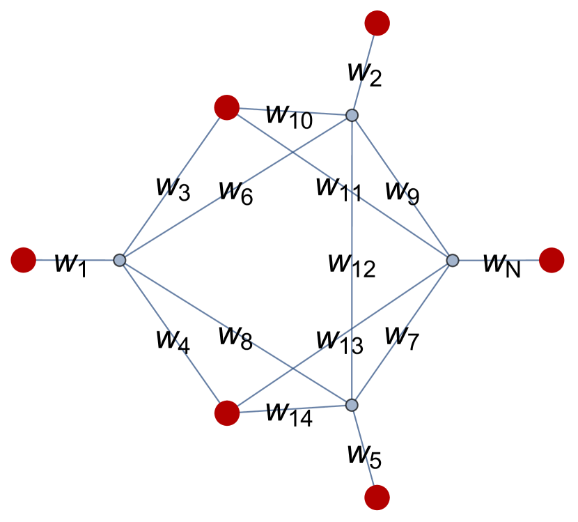
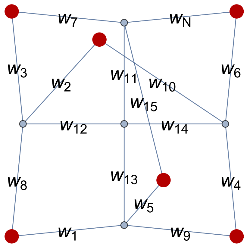
The case is less trivial. There are two star-graph orbits of extreme rays each, see Figure 1 in Appendix B.2. These are extreme rays realizable in , which contains a single bulk vertex. The other extreme rays of involve no bulk vertices. Hence, a convex combination of extreme rays may require a total of bulk vertices at most, which with the terminals and sink gives . This can be further improved as follows. The Bell-pair extreme rays span a subspace of dimension , and the star-graph extreme rays are confined to its -dimensional orthogonal complement. Thus at most star-graph extreme rays are needed to conically span any interior ray of , improving the bound down to . It turns out that the simplicity of the specific extreme-ray graphs for in fact allows us to obtain the definite value . The reason for this is that the -vector of any conical combination of these particular extreme-ray star graphs of can itself also be realized on a star graph. This follows from the observation that all extreme-ray star graphs have identical minimal min-cuts: for every , they all have for and for . Pictorially, this allows one to stack them all on top of each other, adding up their edge weights, so as to realize any combination of these star graphs by a star graph.
This discussion illustrates some strategies for obtaining tighter upper bounds on based on knowledge of extreme rays or the value of . Recall that the number of bulk vertices in is . Regardless of how many extreme rays has, any interior ray may be a conical combination of at most of them. Since we can realize all extreme rays in , we have
| (5.7) |
For instance, since we know , this gives , which is considerably better than the bound given earlier.
We can do even better for by using explicit results about the dimensionality of the span of specific extreme-ray orbits. The Bell pairs take care of dimensions which are not reached by any other extreme ray without introducing any bulk vertices. There is a single orbit that requires , and it consists of extreme rays spanning a subspace of dimension of the remaining of . The largest- orbit spanning the other dimensions has and extreme rays. Hence the worst-case scenario would require graphs with and other with . The total number of vertices carried by a combination of such graphs thus gives the bound . This is better than the more general one attained by (5.7), but requires complete knowledge of all extreme-ray graphs, not just of the number .
Problem 4.
Find tighter bounds on . In particular, does admit an upper bound that is polynomial in ?
6 Computing - and -representations of
To date, there existed no direct or algorithmic procedures for constructing , and all results obtained for up to relied on random/heuristic searches. This section provides two novel systematic methods for computing complete descriptions of . We illustrate them for and describe in detail in Appendix B.777A partial description of was first obtained by [1] and only four years later completed by [14]; the approaches proposed here only take a few hours and additionally obtain provably minimum graph realizations of all extreme rays unknown to date. We also show how partial results for can be obtained by our methods. However, a complete description of appears to be beyond current computational capabilities. Further upgrading our methods to obtain is the subject of work in progress with Bogdan Stoica, to be reported elsewhere. The first method is a general formalization of the strategy used earlier for , whereas the second one constructs starting from knowledge of .
6.1 Method 1
To initialize this method we first set .
Method
-
-
(a)
Generate the -representation P{n+k}-n.ine of using (3.1). Convert this to a -representation P{n+k}-n.ext.
-
(b)
Delete the trivial extreme rays (see Theorem 2) and extract the coordinates corresponding to the variables of the -vectors. Remove redundant rays to obtain the -representation H{n+k}-n.ext of . This is an inner approximation of .
-
(c)
Compute the -representation H{n+k}-n.ine of from H{n+k}-n.ext. Using the ILP method with of Section 5 with , reject facet orbits that are invalid for , continuing until either a facet is rejected or is too large for the ILP to solve.
-
(d)
Test any remaining facet orbits for which the validity is unknown using the proof-by-contraction method of Section 4.1. Generate the full orbits of the facets proved valid, getting a cone HV{n+k}-n.ine which is an outer approximation of .
-
(e)
Compute the extreme rays HV{n+k}-n.ext of HV{n+k}-n.ine. The orbits of -vectors that appeared in P{n+k}-n.ext give extreme rays of by Theorem 2(b). The remaining orbits can be checked by the ILP method of Section 5 with until finding a realization or being too large for the ILP to solve. If all extreme-ray orbits can be realized, then HV{n+k}-n.ine is an -representation of and HV{n+k}-n.ext is its -representation by Proposition 2(c). Otherwise, increment and return to step (a).
Applying Method 1 with , one finds that has facets and extreme rays in dimensions. The resulting has extreme rays in dimensions, and its -representation consists of facets in orbits. All but of them are easily eliminated in step (c) and then proved valid in step (d). These orbits give facets which define HV7-5.ine. Correspondingly, HV7-5.ext has extreme rays falling into orbits. All of the extreme rays are realizable for , so the procedure terminates after a single iteration. Note that we obtain a minimum realization of each extreme ray either in step (a) or (e), wherever it appears first.
The vertex/facet enumeration problems in steps (a), (c) and (e) utilized the code Normaliz888https://www.normaliz.uni-osnabrueck.de on mai20999mai20: Xeon E5-2690 (10-core 3.0GHz), 20 cores, 128GB memory.. Steps (a) and (c) took only a few seconds, and step (e) took minutes. Step (d) was run on a laptop101010Dell XPS 15 7590, i7-9750H CPU @ 2.60GHz, 6 cores, 12 threads, 32GB memory. using a Mathematica implementation111111Available upon request. of the proof-by-contraction method. Most runs were very fast, taking less than seconds, and all finished in no more than minutes. The ILP runs in step (e) were performed with CPLEX121212https://www.ibm.com/analytics/cplex-optimizer , also on mai20, and normally completed in under minute, the longest run taking minutes. The filtration by symmetry generally takes just a few seconds.
Applying Method 1 with we run into computational issues as the vertex/facet enumeration problems quickly become too big to solve with current software and hardware. Nevertheless, we are still able to get useful results using only partial computations. Starting with , has facets and extreme rays in dimensions. The resulting -representation of has extreme rays in dimensions falling into orbits. All orbits can be shown to define orbits of extreme rays of by testing their rank against lifts of inequalities to . Obtaining the -representation of is computationally intractable with presently available algorithms and hardware. To get more extreme ray orbits we set and constructed the -representation of , which has 288 facets in 99 dimensions. It was not possible to do a complete computation of it V-representation. The code Normaliz ran out of memory after about a day of computation, as did other double-description based methods. However we were able to get partial results using the parallel reverse search based method mplrs contained in lrslib131313http://cgm.cs.mcgill.ca/~avis/C/lrs.html which gives output in a stream. After about 6 months of computation with mplrs using between and processors we obtained extreme rays which fall into orbits. By construction, all of these extreme rays are realizable in . Together, these orbits generate about 3 million extreme rays, however orbits become redundant when the full orbits are considered. The non-redundant orbits generate about 1.5 million extreme rays and of the orbits are provably orbits of extreme rays of using lifted inequalities from . Unfortunately it is not possible to compute the facets of such a large cone with current methods. It is important to note that mplrs supports checkpoint/restart and continuing the computation will continue the output stream until a complete -representation is obtained. Being based on reverse search, computer memory is not a constraining factor.
6.2 Method 2
The second method is more sophisticated and involves working with both outer and inner approximations of , refining them until they are equal. The outer approximation is initialized by choosing any set of valid inequalities for , not necessarily facets, whose intersection is full dimensional. The inner approximation is initialized by choosing any feasible set of rays, not necessarily extreme, whose convex hull is also full dimensional. A strong way to initialize the outer approximation is to zero-lift the superbalanced facets of in all possible ways, add to them singleton SA, and generate their full orbits under . By Theorem 5 and Proposition 8, these are all facets of and define a cone OH1-n.ine. For a strong inner approximation, we zero-lift the extreme rays of and generate their full orbits under , which are all extremal in by Proposition 5. Since this is not always full-dimensional, we add the full orbits of the -vectors from Proposition 1 not already included, and remove redundancies. In general, this may only add the single orbit of size generated by . The resulting cone IH1-n.ext is an inner approximation of . Set the iteration counter .
Method
| Outer | Inner | ||
| Compute the -representation OHk-n.ext of OHk-n.ine. Check one extreme ray from each orbit to see if it is realizable by the ILP method of Section 5. If all rays are realizable, then exit. The full orbits of the realizable extreme rays define OHVk-n.ext. | Compute the -representation IHk-n.ine of IHk-n.ext. Apply to it steps (c) and (d) of Method 1, retaining inequalities proved by the contraction method of Section 4.1. If all inequalities are valid, then exit. The full orbits of the valid facets define IHVk-n.ine. | ||
| Merge IHVk-n.ine (and any other known valid inequalities) with OHk-n.ine and remove redundancies to get OH{k+1}-n.ine. | Merge OHVk-n.ext (and any other known realizable rays) with IHk-n.ext and remove redundancies to get IH{k+1}-n.ext. | ||
| Increment and return to the first step of each respective subroutine. | |||
Note that the inner and outer procedures can be run in parallel. After they both finish the first step, the newly computed data are exchanged, improving both the outer an inner approximations. If exit occurs, the corresponding ine and ext descriptions give - and -representations of , respectively. In each subroutine, the second step allows for the incorporation of valid inequalities and/or rays obtained by other means, such as Method 1.
Applying Method 2 with , the starting cones OH1-5.ine and IH1-5.ext respectively consist of facets in orbits (that of singleton SA and of MMI, cf. Appendix B.1), and extreme rays in orbits (cf. Figure 1 in Appendix B.2, and the star orbit).
We start with and describe steps in parallel. In the outer run, OH1-5.ext has extreme rays in orbits, out of which can be shown to be realizable with . Their orbits yield feasible rays defining OHV1-5.ext. In the inner run, IH1-5.ine has facets in orbits, out of which one can show are valid and easily reject the rest. Their orbits yield valid inequalities defining IHV1-5.ine. In the second step it turns out that the outputs of the first step dominate in both cases. So after the merges, OH2-5.ine equals IHV1-5.ine and IH2-5.ext equals OHV1-5.ext.
Setting , in the outer run OH2-5.ext has extreme rays in orbits, all of which are realizable with . Hence exit is triggered, and the algorithm terminates returning OH2-5 as the result for . If we continue the inner run we find that IH2-5.ine has facets in orbits, out of which one can show are valid and easily reject the rest. These are the same orbits as before and so the algorithm exits in the first outer step with .
Conversions between cone representations again require vertex/facet enumeration. Those in the first iteration are immediate. Using Normaliz on mai20, the computations of IH2-5.ine and OH3-5.ext took about seconds and minutes, respectively. The cost of other computations was similar to that of their counterparts in Method 1.
Applying Method 2 with , the starting cones OH1-6.ine and IH1-6.ext are in dimensions and respectively consist of facets in orbits and extreme rays in orbits. We start with . Again we have to be satisfied with partial computation using mplrs as the problem is too large for current computational methods to terminate in reasonable time. In the outer run after about 10 days of computation we obtained extreme rays from OH1-6.ext belonging to 3288 distinct orbits. None of these 3288 orbits can be ruled out using lifted inequalities (by construction, because they come from OH1-6.ine), which means a priori we have literally 3288 candidates. Using a set of heuristically generated inequalities that we were able to prove valid via the contraction method, we reduce this list down to 55 candidates. Of these, orbits are easily seen to correspond to lifts of extreme rays. Using CPLEX and the ILP method we found minimum realizations of all orbits: in (lift of a Bell pair), in ( are lifts of star graphs), in , in , in and in . All of these extreme rays are thus extreme rays of by construction. Note that only those realizable in for could have appeared in the Method 1 run described. As noted for Method 1, the computation of OH1-6.ext can be continued with additional new orbits being produced as a stream until the computation is completed. In the inner run, the computation of the -representation of IH1-6.ext was too big to produce any useful output in two weeks of computation with mplrs using processors.
6.3 Comparison of Method 1 and Method 2
Although the inner steps of Method 2 may appear similar to Method 1, they are in fact quite distinct. In the latter, the starting cone H{n+2}-n.ext only contains -vectors realizable in . Many of these will be non-extremal in and therefore absent from IH1-n.ext. Among those which are extremal, some may not be obtainable by zero-lift and thus not included in IH1-n.ext either. On the other hand, IH1-n.ext contains all extreme rays of coming from zero-lifts. These will generally include plenty which are not realizable in and hence not be contained in H{n+2}-n.ext. For example, for , IH1-6.ext includes zero-lifts of extreme rays in the orbits of which are realizable in with (see Table 3 in Appendix B.2), none of which can possibly be in H8-6.ext.
Both methods may run into fundamental and/or practical issues. For , one is fortunate that the contraction method successfully proves valid the facet orbits of . However, it remains a logical possibility that for larger this proof method is not a necessary condition for validity of some facets of (cf. Problem 3 at the end of Section 4.1). Specifically in Method 1, it so happens that all rays in HV7-5.ext are realizable using the ILP of Section 5. For larger , in practice it could be that even if all rays at step (e) were realizable, the value of required could be too high for the ILP to be solved. Without good bounds on , this possibility cannot be easily eliminated. Alternatively, it could be that some rays are indeed not realizable, meaning that the facet description in HV{n+k}-n.ine is incomplete. This would require incrementing and at least one further iteration. As for Method 2, we unfortunately have no proof of convergence using the strong starting inputs suggested without the option to generate and add additional valid inequalities and/or feasible rays in the second step. There are various heuristic methods available to generate such additional inputs. Another complication that affects these methods is the need to solve large convex hull/facet enumeration problems. All of these issues arise in one form or another in both methods already in the study of .
The successful termination of either method relies on the finding of an /-representation of an inner/outer approximation of containing all of its facets/extreme rays. For instance, observe that in Method 1 all facets of were already discovered in step (a) and computed explicitly in step (c) (along with other non-valid inequalities) from for just . Similarly, Method 2 converged more easily through an inner approximation IH1-5 whose -representation also contained all facets of . That is easier to obtain from an -representation of an inner approximation is no accident. This is because smaller for is needed to span all facets than to realize all extreme rays of . This motivates the definition of as the smallest integer such that the -representation of contains all facets of .
It is easily seen that for and that for larger . For , the cone turns out to miss some facets of , but does contain them all as we have seen in Method 1. This shows that , contrasting with the extreme rays, which have . More generally, when Method 1 terminates, we have and a minimum realization of each extreme ray, from which one also obtains . This makes the importance of manifest and motivates the following problem:
Problem 5.
Find tighter bounds on . In particular, does admit an upper bound that is polynomial in ?
7 Conclusion
Many of the important questions about the HEC remain open. As stated formally throughout the paper in Problems 1 through 5, these include obtaining an explicit description of either the - or -representation of , and finding the complexity of testing feasibility of rays and validity of inequalities. The current bounds on the size of the complete graph that can realize all extreme rays of seem far from being tight, at least according to the limited experimental results that we have. Similarly, our findings suggest that much smaller graphs may be sufficient to span all facets of , which strongly motivates understanding better the relative complexity of the - and -representations of the HEC. Ultimately, one would hope to obtain a more fundamental understanding of the HEC, such as in the form of the structural conjectures put forward recently in [8, 10, 16, 9]. In this work, we have laid the foundations for further exploration of these key questions and provided some useful tools for testing and proving such ideas. Additionally, we have provided sharp computational tools which allowed us to completely describe after just a few hours of computation and produce significant new results for .
Acknowledgments
We thank Patrick Hayden, Temple He, Veronika Hubeny, Max Rota, Bogdan Stoica and Michael Walter for useful discussions. We would also like to thank an anonymous referee for many comments and suggestions for improving the paper.
References
- Bao et al. [2015] Bao N, Nezami S, Ooguri H, Stoica B, Sully J, Walter M (2015) The Holographic Entropy Cone. JHEP 09:130, doi:10.1007/JHEP09(2015)130, arXiv:1505.07839
- Bao et al. [2020a] Bao N, Cheng N, Hernández-Cuenca S, Su VP (2020a) A Gap Between the Hypergraph and Stabilizer Entropy Cones. arXiv:2006.16292
- Bao et al. [2020b] Bao N, Cheng N, Hernández-Cuenca S, Su VP (2020b) The Quantum Entropy Cone of Hypergraphs. SciPost Phys 9(5):067, doi:10.21468/SciPostPhys.9.5.067, arXiv:2002.05317
- Brouwer et al. [2013] Brouwer AE, Mills C, Mills W, Verbeek A (2013) Counting families of mutually intersecting sets. Electron J Comb 20(2), doi:10.37236/2693
- Chen et al. [2022] Chen B, Czech B, Wang Zz (2022) Quantum information in holographic duality. Rept Prog Phys 85(4):046001, doi:10.1088/1361-6633/ac51b5, arXiv:2108.09188
- Cunningham [1985] Cunningham WH (1985) On submodular function minimization. Comb 5(3):185–192, doi:10.1007/BF02579361
- Czech and Dong [2019] Czech B, Dong X (2019) Holographic Entropy Cone with Time Dependence in Two Dimensions. JHEP 10:177, doi:10.1007/JHEP10(2019)177, arXiv:1905.03787
- Czech and Shuai [2021] Czech B, Shuai S (2021) Holographic Cone of Average Entropies. arXiv:2112.00763
- Czech and Wang [2022] Czech B, Wang Y (2022) A holographic inequality for regions. arXiv:2209.10547
- Fadel and Hernández-Cuenca [2022] Fadel M, Hernández-Cuenca S (2022) Symmetrized holographic entropy cone. Phys Rev D 105(8):086008, doi:10.1103/PhysRevD.105.086008, arXiv:2112.03862
- Fujishige [2005] Fujishige S (2005) Submodular Functions and Optimization, Ann. Discrete Math., vol 58. Elsevier, doi:10.1016/S0167-5060(13)71057-4
- Hayden et al. [2013] Hayden P, Headrick M, Maloney A (2013) Holographic Mutual Information is Monogamous. Phys Rev D 87(4):046003, doi:10.1103/PhysRevD.87.046003, arXiv:1107.2940
- He et al. [2020] He T, Hubeny VE, Rangamani M (2020) Superbalance of Holographic Entropy Inequalities. JHEP 07:245, doi:10.1007/JHEP07(2020)245, arXiv:2002.04558
- Hernández-Cuenca [2019] Hernández-Cuenca S (2019) Holographic entropy cone for five regions. Phys Rev D 100(2):026004, doi:10.1103/PhysRevD.100.026004, arXiv:1903.09148
- Hernández-Cuenca et al. [2019] Hernández-Cuenca S, Hubeny VE, Rangamani M, Rota M (2019) The quantum marginal independence problem. arXiv:1912.01041
- Hernández-Cuenca et al. [2022] Hernández-Cuenca S, Hubeny VE, Rota M (2022) The holographic entropy cone from marginal independence. JHEP 09:190, doi:10.1007/JHEP09(2022)190, arXiv:2204.00075
- Hubeny et al. [2018] Hubeny VE, Rangamani M, Rota M (2018) Holographic entropy relations. Fortsch Phys 66(11-12):1800067, doi:10.1002/prop.201800067, arXiv:1808.07871
- Hubeny et al. [2019] Hubeny VE, Rangamani M, Rota M (2019) The holographic entropy arrangement. Fortsch Phys 67(4):1900011, doi:10.1002/prop.201900011, arXiv:1812.08133
- Kleitman and Markowsky [1975] Kleitman D, Markowsky G (1975) On Dedekind’s Problem: The Number of Isotone Boolean Functions. II. Trans Am Math Soc 213:373–390, doi:10.2307/1998052
- Nezami and Walter [2020] Nezami S, Walter M (2020) Multipartite Entanglement in Stabilizer Tensor Networks. Phys Rev Lett 125:241602, doi:10.1103/PhysRevLett.125.241602, arXiv:1608.02595
- Nielsen and Chuang [2010] Nielsen MA, Chuang IL (2010) Quantum Computation and Quantum Information. Cambridge University Press, doi:10.1017/CBO9780511976667
- Pippenger [2003] Pippenger N (2003) The inequalities of quantum information theory. IEEE Trans Inf Theory 49(4):773–789, doi:10.1109/TIT.2003.809569
- Rangamani and Takayanagi [2017] Rangamani M, Takayanagi T (2017) Holographic Entanglement Entropy, Lect. Notes Phys., vol 931. Springer, doi:10.1007/978-3-319-52573-0, arXiv:1609.01287
- Ryu and Takayanagi [2006] Ryu S, Takayanagi T (2006) Holographic derivation of entanglement entropy from AdS/CFT. Phys Rev Lett 96:181602, doi:10.1103/PhysRevLett.96.181602, arXiv:hep-th/0603001
- Schrijver [1999] Schrijver A (1999) Theory of Linear and Integer Programming. Wiley Series in Discrete Mathematics & Optimization, Wiley
- Van Raamsdonk [2010] Van Raamsdonk M (2010) Building up spacetime with quantum entanglement. Gen Rel Grav 42:2323–2329, doi:10.1142/S0218271810018529, arXiv:1005.3035
- Walter and Witteveen [2020] Walter M, Witteveen F (2020) Hypergraph min-cuts from quantum entropies. arXiv:2002.12397
Appendix A Origins and importance of the HEC in physics
The tools of convex geometry have long been applied to systematically study entropy inequalities, from those obeyed by the Shannon entropy of random variables in classical probability distributions, to the ones that the von Neumann entropy of marginals of density matrices of quantum states satisfy [22]. As a measure of quantum entanglement, the study of the latter has proven to be of paramount importance to the development of the field of quantum information theory and, more generally, to the understanding of correlations in quantum physics [21].
Although the finding of universal inequalities obeyed by general quantum states has been elusive, significant progress has been made by the restriction of the domain of the entropy function to specific subclasses of quantum states of special relevance for which additional tools are at hand. In the context of quantum gravity and holography, one very important such class of quantum states are those which admit a semi-classical description in terms of a theory of gravity on a higher-dimensional spacetime. More specifically, in such cases, the Anti-de Sitter/Conformal Field Theory (AdS/CFT) correspondence asserts that a holographic state of the CFT, defined on a boundary spacetime , has a gravitational bulk dual on a spacetime with as its conformal boundary, . In the bulk, quantum entanglement of the CFT state acquires a geometric character which has been understood to play a fundamental role in the very emergence of spacetime itself [26]. These findings rely on the much celebrated Ryu-Takayanagi (RT) prescription [24, 23], according to which the von Neumann entropy of a spatial boundary region is given holographically by
| (A.1) |
where is Newton constant, is Planck constant, and the minimization is over bulk hypersurfaces in a time slice homologous to relative to , i.e., subject to the condition . This geometric character that the von Neumann entropy acquires in the bulk turns out to place strong constraints on the allowed entanglement structures of holographic states. In a remarkable paper, Bao et al. [1] initiated a systematic exploration of these constraints with the objective of formalizing a set of conditions on quantum states to posses holographic duals. These were formulated as entropy inequalities satisfied by the RT formula, defining the facets of a polyhedral cone which was coined as the HEC.
More precisely, the HEC is a family of polyhedral cones labelled by an integer , all related by projections from larger to smaller . Their work laid the ground for the finding of new results about the HEC [14, 7, 13], and also lead to further generalizations and explorations of their methods [17, 18, 15, 3, 27, 2]. Most of these developments relied on two remarkable results of [1]: a proof of equivalence between holographic entropies obtained by the RT formula and minimum cuts on weighted graphs141414Intuitively, the graph provides a discrete tessellation of the manifold which encodes sufficient information about its metric in the form of edge weights, with minimal surfaces and their areas becoming minimum cuts and their weights, respectively – see [1]., and the invention of a combinatorial method to prove the validity of holographic entropy inequalities that we will review in Section 4. Crucially, their graph models allow for a complete study of the HEC from a purely combinatorial viewpoint without reference to the geometric RT formula or quantum physics.
Appendix B Extremal structure of for
Here we summarize the extremal structure of for all by showing representatives of every orbit of both facets and extreme rays. Representatives of each orbit are picked as their lexicographical minimum.151515The only exception to this is inequality 1 in Table 2, which is chosen for symmetry reasons. For extreme rays, we also present their minimum realizations, exhibiting graphs where only edges of nonzero weight are shown. At every , we only include elements which are genuinely new and not coming from zero-liftings. This is because these should always be included – by Proposition 5 the zero-lift of rays preserves all extreme rays, while by Theorem 5 the zero-lift of inequalities preserves all superbalanced facets. As for SA, Proposition 8 guarantees that precisely only instances involving just singletons in give rise to facets. It will thus be convenient to present results in increasing order of .
B.1 Facets
At one just has one single-element orbit of a nonnegativity facet,
| (B.1) |
For , the cone is a simplex with facets in a single orbit of SA,
| (B.2) |
Lifting to , one gets facets in the orbit of the trivial zero-lift of SA. The cone becomes again a simplex due to the appearance of the new, totally symmetric facet of MMI
| (B.3) |
There are no genuinely new inequalities for . The trivial zero-lift of the SA facet gives a length- orbit. Every zero-lift of (B.3) in fact lands on the same MMI orbit, which consists of another facets. In total, thus has facets and is not simplicial anymore.
It is at that begins to exhibit a richer structure. The trivial zero-lift of SA now contributes an orbit of facets. The trivial zero-lift of MMI gives an orbit with facets. There is now another inequivalent zero-lift of MMI which gives an orbit of length . Besides these, there are orbits of genuinely new facets, given in Table 2.
In order, these give rise to orbits of lengths , , , and . Together with the facets coming from SA and MMI, there are a total of inequalities in the -representation of . Other than inequality 1, usually referred to as cyclic due to its symmetry under which is manifest in the given representative, these inequalities are poorly understood.
-
1.
-
2.
-
3.
-
4.
-
5.
B.2 Extreme rays and minimum graph realizations
Extreme rays and their minimum realizations in will be provided. Extreme rays will be labelled by a tuple , where is just an integer counting orbits at fixed and by listing their representatives lexicographically. Notice that counts the number of bulk vertices needed in the minimum representation, plus the sink. For clarity, -vector entries will be separated by a semicolon whenever the cardinality of increases.
At there is a single extreme ray with minimum realization the Bell pair in Figure 1,
| (B.4) |
The cone has just the length- orbit of zero-lifts of the Bell-pair extreme ray . For , the Bell-pair zero-lift now gives an orbit of extreme rays. A new totally symmetric extreme ray appears. It has a star-graph minimum realization shown in Figure 1 and reads
| (B.5) |
Lifting to we get orbits of extreme rays from and another from . A genuinely new length- orbit of extreme rays appears,
| (B.6) |
which again has a star graph as minimum realization, as shown in Figure 1.

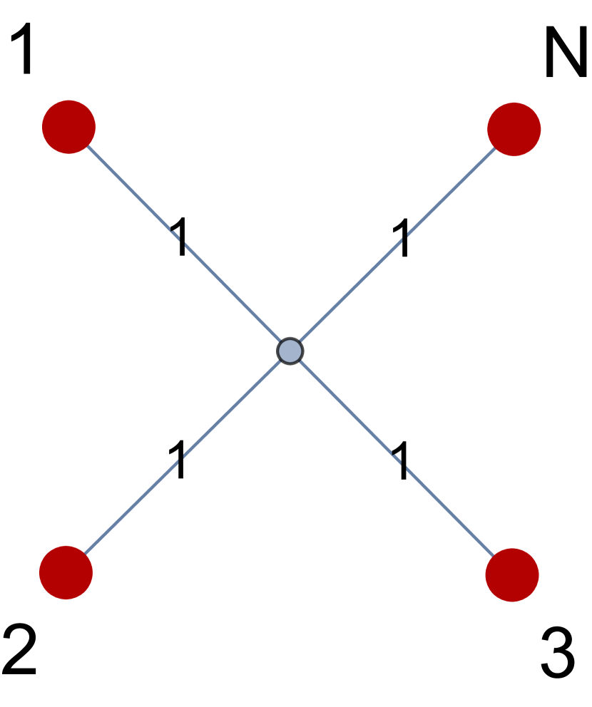
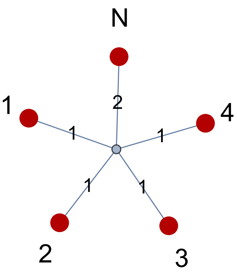
At , lifted extreme rays become a minority. Extreme rays , and respectively zero-lift to orbits of lengths , and , totaling just extreme rays. It turns out has in total, so all the others are genuinely new ones. They fall into orbits, which we now present by increasing number of bulk vertices needed in their minimum realization. There are distinct orbits of extreme rays realizable in a star graph,
| (B.7) | ||||
with respective orbit lengths , , and . They can all be represented on the star graph shown in Figure 2(1), with appropriate weight assignments as specified in Table 3. There are orbits which require bulk vertices,
| (B.8) | ||||
with respective orbit lengths , , , , and . These can be represented on graphs in Figures 2(2) to 2(5) following Table 3. There are orbits which require bulk vertices,
| (B.9) | ||||
with respective orbit lengths , , and . These are realizable in graphs in Figures 2(6) to 2(8) following Table 3.
Finally, there is an orbit of length with bulk vertices,
| (B.10) |
and another one of length with bulk vertices,
| (B.11) |
These are respectively realizable in graphs in Figures 2(7) and 2(8) following Table 3.
In summary, consists of extreme rays in orbits, of which lie in orbits new to . Note that apart from the Bell pair in Figure 1, there are no edges between terminals in any of the minimum extreme-ray representations. Each is planar except for in Figure 2(8), which can be embedded on a torus. Terminals have degree at most .
Appendix C Miscellaneous examples
Convexity of and :
For , consider extreme rays and the zero-lift of , both of which are realizable in . Using the ILP method in Section 5 we can determine that their sum is not. Therefore, neither nor is convex without the convex operator applied. The minimum realization of their sum is in , and has edges with respective weights .
Extreme rays of and :
For in , consider these three feasible pairs:
Here is an extreme ray of . However, its coordinates have , so the latter cannot be an extreme ray of and hence of either (cf. Theorem 2(b)).
| Extreme Ray | Graph | Terminal Edges | Edge Weights | ||||||||||||||||||||