SPATIO-TEMPORAL GRAPH-RNN FOR POINT CLOUD PREDICTION

Abstract

In this paper, we propose an end-to-end learning network to predict future frames in a point cloud sequence. As main novelty, an initial layer learns topological information of point clouds as geometric features, to form representative spatio-temporal neighborhoods. This module is followed by multiple Graph-RNN cells. Each cell learns points dynamics (i.e., RNN states) by processing each point jointly with the spatio-temporal neighbouring points. We tested the network performance with a MINST dataset of moving digits, a synthetic human bodies motions and JPEG dynamic bodies datasets. Simulation results demonstrate that our method outperforms baseline ones that neglect geometry features information.

Index Terms—  Point Cloud, Graph-based representation learning, Point-based models.

1 Introduction

Point clouds (PCs) sequences provide a flexible and rich geometric representation of volumetric content, quickly becoming an attractive representation for applications such as autonomous driving [1], mixed reality application services [2], cultural heritage [3]. This has motivated intense research toward PC processing, with strong focus on static PCs, leaving the dynamic PC processing (DPC) usually overlooked. In this work, we focus on DPC processing and specifically on the prediction of point cloud dynamics. Namely, given PC frames $P_{1},P_{2},\ldots,P_{t}$ we are interested in predicting $\hat{P}_{t+1}$, with no prior knowledge on the ground truth $P_{t+1}$.

In the current literature, DPCs processing has been approached from two overlapping directions: (1) motion estimation (ME) and motion compensation (MC) for PC compression; (2) 3D motion flow prediction (usually deep-learning based) for high-level tasks (e.g., gesture recognition). Both approaches share a common challenge: extraction of temporal correlations between sequential PC frames, challenged by the irregular structure and by the lack of explicit point-to-point correspondence. At the same time, these two directions have fundamentally different goals and setups: the former aimed at extracting the motion vector from two known consecutive frames, the latter focused on a much more challenging task of prediction of future unknown PC frames. This requires learning both the short- and long-term PC trajectory. Another key difference lies in the developed solutions: ME mainly addresses the lack of correspondence either by projecting the 3D PC into the 2D domain and adopting mature algorithms from 2D video compression [4] or by developing 3D ME methodologies, preserving the volumetric information of the PCs [5, 6, 7].

Motion flow prediction involves deep learning processing instead, the irregular and unordered structure of PC prevents the immediate adoption of convolution neural networks. Within this framework, PointNet [8] has become a pillar work for static PC processing, capable of learning directly from raw PC data with no pre-processing: each point in the PC is processed independently and all point features are aggregated subsequently. Modeling points independently achieves permutation invariance, but at the price of losing the geometric relationship between points, a key piece of information in PCs that we aim at retaining. To learn the dynamic behavior of sequential data, recent works [9, 10, 11] has extended PointNET architecture to recurrent neural networks (RNNs), predicting the 3D motion flow of PCs. In the PointRNN model [11], for example, each point is processed individually by RNN cells with the output being the point state (i.e., the motion of the point). Each point state is extracted by aggregating state information from neighboring points. The neighborhood of a point of interest is defined as the $k$ nearest neighbor ($k$-nn) points in the previous frame, where the proximity is measured based on the point coordinates. This methodology inherits the ability to capture the dynamic behavior of sequential data from RNN models, as well as permutation invariance from PointNet architecture. However, it suffers from the same shortcoming of PointNet: lack of geometric relationship between points which may lead to i) loss of structure during PC reconstruction; ii) poor $k$-nn neighborhood as grouping points only based on coordinates might connect two points close in space but not belonging to the same segment, hence not sharing the same motion.

In this paper, we seek to bridge the gap between graph-based representations of PC [12, 13, 14] and deep learning motion flow prediction. We propose an end-to-end architecture, where an initial pre-processing step learns topological information of PC as geometric features, and leverage on those learned features to form more representative local neighborhoods of points than PointRNN models. From the learned features, a Graph-RNN constructs spatio-temporal $k$-nn graphs. This results in spatio-temporal aggregation of points that share common local features instead of only points coordinates. The temporal correlations from the spatio-temporal graph are aggregated to learn point states. The Graph-RNN learns points states, which retain the model dynamic information over time and allow to model long-term point trajectory. The proposed solution has been validated on moving MNIST point cloud dataset used in the literature [11] as well as on a synthetic human b odies motions and JPEG dynamic bodies datasets [15, 16]. Simulation results demonstrate that our method can make correct PC predictions showing its ability to accurately group points and model long-term relationships while preserving the spatial structure.

2 Proposed Method

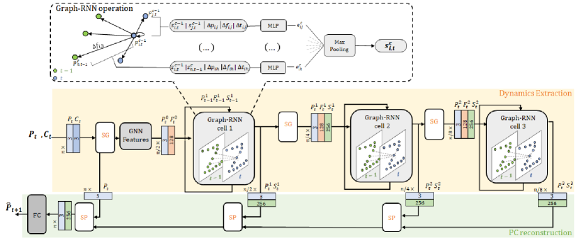
Fig. 1: Scheme of the complete hierarchical architecture, composed of four main components: Sampling and Grouping (SG); GNN for Features Learning ; Graph-RNN (diagram of it’s operation included in dashed area) ; States propagation (SP).

We denote a point cloud frame consisting of $n$ points by $P_{t}=\{p_{1,t},p_{2,t},\ldots p_{n,t}\}$ with $p_{i,t}\in\mathbb{R}^{3}$ being the euclidean coordinates of point $i$ in $P_{t}$. Each PC has additional attributes (i.e., point color) denoted by $C_{t}=\{c_{1,t},c_{2,t},\ldots c_{n,t}$, with $c_{i,t}\in\mathbb{R}^{3}$ the associated color component. Given a point cloud sequence $\mathcal{P}=(P_{1},P_{2},...,P_{T})$ composed by $T$ frames and additional attributes $\mathcal{C}=(C_{1},C_{2},...,C_{T})$, our goal is to predict the coordinates of future point clouds $\hat{P}_{T+1},\ldots,\hat{P}_{T+Q}$, with $Q$ being the prediction horizon.

To reach this goal, we proposed an interactive framework (Fig. 1), which allows us to predict future trajectories of points via RNN cells. At each iteration, the network processes one input frame $P_{t}$ and its color attribute $C_{t}$ giving as output the prediction of the successor frame $\hat{P}_{t+1}$. The architecture is composed of two phases: i) a dynamics extraction (DE) phase where the PC dynamic behaviour is captured in the form of point states, ii) a PC reconstruction phase where the states are concatenated and used to output the PC prediction. In the DE phase, as key novelty, we pre-process the point cloud to extract point features that carries local geometry information. Specifically, a initial graph neural network (GNN) module transforms the 3D space into an higher dimensional feature space and sends the output to a Graph-RNN cell. In each cell, each point is processed independently to preserve permutation invariance. Specifically, each point state is extracted by aggregating information from its $k$-nn neighborhood. After the Graph-RNN cells, the PC reconstruction phase begins. The states are propagated and processed by a fully connected layer (FC) to estimate motion vectors, used to predict the next frame $\hat{P}_{t+1}$. Before each Graph-RNN cell, the point cloud is down-sampled. It is then up-sampled to its original size before the final FC layer. The down-sampling and up-sampling blocks are implemented as in [17] and we refer the readers to Section A of the Appendix. for further information. The intuition for the design hierarchical architecture is to learn states at multiples scales: the first Graph-RNN cell handles a dense PC and learns states in local regions (corresponding to local motions), while the last Graph-RNN cell learns states in a sparser PC with more distant points included in the neighborhood (corresponding to more global motions).

We now provide more details on the key modules that are part of our contributions: GNN-based pre-processing and Graph-RNN cells.

2.1 GNN for Feature Learning

Given $P_{t}$ and $C_{t}$ as input, we construct a directed $k$-nn coordinate graph $\mathcal{G}^{C}_{t}=(P_{t},\mathcal{E}^{C}_{t})$ with vertices $P_{t}$ and edges $\mathcal{E}^{C}_{t}$. Each edge connects a point to its $k$-nearest neighbors based on euclidean distance. The graph includes self-loop, meaning each point is also connected to itself. Given the coordinate graph as input, the GNN module learns the geometric features $F_{t}\in\mathbb{R}^{n\times d_{f}}$. The GNN is composed of $L$ layers, and in each layer features are learned by aggregating information along the edges.

Inspired by [12], we learn the features by taking into account the relationship (similarity) between neighboring points. At the $l$-th layer of the GNN, the edge features $e^{l}_{i,j}$ are learned for each point $i$ and for each neighboring node $j$. This is done by concatenating the input point feature $f_{i,t}^{l-1}$ and the point coordinates $p_{i,t}$, with the geometry and color displacement/difference between the points $i$ and $j$ ($\Delta p_{ij}$, $\Delta c_{ij}$, respectively). We then apply a symmetric aggregation operation on the edge features associated with all the edges emanating from each point. More formally, the edge features ($e^{l}_{i,j}$) and the output point features ($f^{l}_{i}$) are obtained as follows:

$$e^{l}_{i,j} =h_{F}^{l}(f_{i,t}^{l-1}\;;p_{i,t}\;;\Delta p_{ij}\;;\Delta c_{ij})$$ (1)

$$f^{l}_{i} =\operatorname*{\textit{MAX}}_{j:(i,j)\in\mathcal{E}^{C}}\big{\{}e^{l}_{i,j}\big{\}}$$ (2)

where $h_{F}$ is a nonlinear learnable function that can be implemented with a multi layer perceptron (MLP), ’;’ identifies the concatenation operation and $\operatorname*{\textit{MAX}}$ represents the element-wise max pooling function. Note that for the first layer $l=1$, we set $f_{i,t}^{0}$ as a null entry and the output of the $L$-th layer is the geometric feature $F_{t}=[f_{1,t}^{L},f_{2,t}^{L},\ldots,f_{n,t}^{L}]$.

2.2 Graph-RNN

Each Graph-RNN cell $c$ receives the feature $F_{t}^{c-1}$ and $P_{t}^{c-1}=[p^{c-1}_{1,t},p^{c-1}_{2,t},\ldots,p^{c-1}_{n,t}]$ as input, with $F_{t}^{0}$ being the output of the previous GNN module. Given it iterative nature, the Graph-RNN cell takes into account the input and also its own output $(P^{c}_{t-1},F^{c}_{t-1},S^{c}_{t-1})$ calculated at the previous interaction $(t-1)$. The cell extracts the inner state $S_{t}^{c}=[s^{c}_{1,t},s^{c}_{2,t},\ldots,s^{c}_{n,t}]\in\mathbb{R}^{n\times d_{s}}$, with $s^{c}_{i,t}$ being the state of point $p^{c}_{i,t}$, representative of the point dynamic behavior. The new state is added to the unchanged coordinates $P^{c-1}_{t}$ and features $F^{c-1}_{t}$ and outputted as $(P^{c}_{t},F^{c}_{t},S^{c}_{t})$. Similarly to [11], we consider three sequential Graph-RNN cells.

The Graph-RNN operation is the depicted in Fig. 1 (dashed box). As first step, we compute a spatio-temporal feature graph $\mathcal{G}^{F}_{t}$, in which each point is connected to $k$ nearest neighbors based on the feature distance. Specifically, for each input point $p_{i,t}^{c-1}$, we compute the pairwise distance between $f_{i,t}^{c-1}$ and features of other points $f_{j,t}^{c-1}$ (features input) and $f_{j,t-1}^{c}$ (features from points in the past PC). We force our implementation to take the equal number of points $k$ from $P^{c-1}_{t}$ as from $P^{c}_{t-1}$ to avoid a one-side selection. In details, this is a spatio-temporal graph since each point is connected to points in the same PC (spatial relationship) and points in the past PC (temporal relationship). Once the features graph is constructed, we learn edge features similarly to the GNN module. For the edge $(i,j)$, we concatenate the state of point $i$ ($s_{i}$), the state of point $j$ ($s_{j}$), and the coordinate, the feature and the time displacement ($\Delta_{p_{i,j}},\Delta_{f_{i,j}}\Delta_{t_{i,j}}$) between the two points. The concatenation is then processed by a shared MLP $(h_{S})$. All edge features are then max pooled to a single representation into the update state $s_{i,t}$. Formally,

$$e^{c}_{i,j} =h_{S}^{c}(s^{c-1}_{i,t};s^{c^{\prime}}_{j,t^{\prime}};\Delta p_{ij};\Delta f_{ij};\Delta t_{ij})$$ (3)

$$s^{c}_{i,t} =\operatorname*{\textit{MAX}}_{j:(i,j)\in\mathcal{E}^{F}}\big{\{}e^{c}_{i,j}\big{\}}$$ (4)

When learning output states $S^{c}_{t}$, the Graph-RNN cell considers the states in the previous frame $S^{c}_{t-1}$. This means that the network learns point movements taking into consideration the previous movements of points, allowing the cell to retain temporal information. The states act as a memory retaining the history of movements and enabling for network to model long-term relationships over time.

2.3 Training

The architecture in Fig. 1 has multiple learnable parameters (in GNN, Graph-RNN, FC), which are end-to-end trained. We consider a supervised learning settings in which the loss function relates to the prediction error between ground truth point cloud $P_{t}$ and the predicted one $\hat{P}_{t}$. To evaluate the prediction error, we adopt the Chamfer Distance (CD) and Earth Moving Distance (EMD) between $P_{t}$ and $\hat{P}_{t}$ evaluated as follows [18]:

$$d_{CD}(P,\hat{P}) =\sum_{p\in P}\min_{\hat{p}\in\hat{P}}||p-\hat{p}||^{2}+\sum_{p\in\hat{P}}\min_{p\in P}||\hat{p}-p||^{2}$$ (5)

$$d_{EMD}(P,\hat{P}) =\min_{\theta:P\xrightarrow{}\hat{P}}\sum_{p\in P}||p-\theta(p)||^{2}$$ (6)

where $\theta:P\xrightarrow{}\hat{P}$ is a bijection. The loss function used to train the network then is given by the sum of CD and EMD distances, namely $\mathcal{L}(P,\hat{P})=d_{CD}(P,\hat{P})+d_{EMD}(P,\hat{P})$.

3 Experiments

We implemented the end-to-end network described in Sec.2 in the case of $L=3$ layers within the GNN module and $C=3$ RNN cells. We consider both short-term and long-term prediction, with the former predicting only one future frame $Q=1$ (ground truth frame $P_{t}$ is used to predict the next frame $\hat{P}_{t+1}$) while the latter predicting $Q=T/2$ future frames with $\hat{P}_{t}$ being used to predict the next frame $\hat{P}_{t+1}$. As baseline models we consider: (1) Copy Last input model which simply copies the past PC frame instead of predicting it; (2) PointRNN ($k$-nn) model [11], which neglects geometry information. In our experiments, we considered the following datasets:  Moving MNIST Point Cloud, created by converting the MNIST dataset of handwritten digits into moving point clouds, as in [11], each sequence contains 20 ($T$) frames with either 128 (1 digit) or 256 points (2 digits) .
Synthetic Human Bodies Activities, synthetically generated by us following [15] using the online service Mixamo [19] in combination with the 3D animation software Blender [20].
JPEG Pleno 8i Voxelized Full Bodies, four benchmark sequences: longdress, loot, redandblack, and soldier [16].
In the two last datasets, each PC sequence contains 12 ($T$) frames and is downsampled to $4,000$ points. The network is trained with the Synthetic Human Bodies Activities dataset, which provides different levels of movements (walking, jumping, dancing, etc) and tested on both datasets.

To better understand our system, we visualized the learned features for one PC from the Synthetic Human Bodies dataset. Fig. 2 depicts in sequence: the point cloud, the learned features $F_{t}$, the output state $S_{t}$, the reconstructed motion vector $M_{t}$, and the predicted PC. Principal Component Analysis (PCA) is used for the features visualization. It is worth noting that features can segment the PC into regions sharing similar topology (leading to meaningful neighborhood in the features graph) and states are able to capture the movement of moving parts –e.g., leg and foot taking a step forward. The states are directly translated into motion vectors, used to make accurate prediction of the future frame. A more complete comparison can be deduced from Fig. 3, depicting resultant and ground truth PCs for the MINST dataset. Interestingly, the predicted digits are sharper and clearer in the Graph-RNN prediction than the PointRNN. This demonstrates that while both models capture the correct motion, the Graph-RNN is better at preserving the spatial structure over time. This is a direct effect from learning geometric features.

We now provide more quantitative results for both the MNIST dataset (Table 1), and the Synthetic Human Bodies and JPEG datasets (Table 2). For all datasets, the proposed Graph-RNN outperforms the PointRNN solution as well as the baseline solutions. From Table 1, it is worth noting that the hierarchical implementation (in which PC is sampled between RNN-cells) leads to a better prediction compared to the “Basic” (not down-sampled) counterpart. This is expected as the hierarchical structure learns states at different resolution. Finally, the model “Graph-RNN (color)” considers the color attributes when learning features, resulting in a more meaningful spatio-temporal neighborhood [21] and therefore in a better prediction.

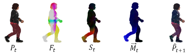
Fig. 2: Multiple representation steps of short-term prediction Graph-RNN on Bodies dataset

Fig. 3: Visualization of moving MNIST point cloud prediction with two moving digits (Hierarchical architecture)

MINST
		Long-term Prediction
		One Digit		Two digit
Method		CD	EMD	CD	EMD
Copy last input		262.46	15.94	140.14	15.8
	PointRNN	5.86	3.76	22.12	7.79
Basic	GraphRNN	2.43	2.40	13.66	6.13
	PointRNN	2.25	2.53	14.54	6.42
Hierarchical	Graph-RNN	1.22	1.86	4.62	3.97

Table 1: Prediction error of PointRNN and Graph-RNN with $k$-nn on the moving MNIST point cloud dataset.

	Synthetic Human Bodies				JPEG Dynamic Bodies
	Short-Term		Long-Term		Short-Term		Long-Term
Method Hierarchical	CD	EMD	CD	EMD	CD	EMD	CD	EMD
Copy Last Input	0.161	0.153	0.247	0.408	0.0004	0.029	0.0020	0.058
PointRNN	0.007	0.104	0.066	0.257	0.0005	0.034	0.0024	0.082
Graph-RNN	0.005	0.078	0.077	0.248	0.0003	0.026	0.0018	0.074
Graph-RNN (color)	0.004	0.071	0.063	0.219	0.0003	0.025	0.0014	0.053

Table 2: Prediction error of PointRNN and Graph-RNN on the Synthetic Human Bodies and JPEG datasets

4 Conclusion

This paper proposes end-to-end learning network to process dynamic PCs and make accurate predictions of future frames. We design a Graph-RNN cell that can leverage learned features, describing the local topology, to form spatio-temporal graphs, from where temporal correlations can be extracted. Experimental results demonstrate the network’s ability to model short and long-term motions while preserving the spatial structure.

This supplementary material provides additional details of the proposed framework.

In Sec A we provide details on hierarchical structure. Sec B includes additional information of the datasets used in the experiments. Sec C provides implementation details of the architecture. Lastly Sec D provides visualization and analysis of additional experiments.

Appendix A Hierarchical structure details

In this paper, we proposed a hierarchical architecture, where before each Graph-RNN cell the point cloud and the associated components are down-sampled by a Sampling and Grouping (SG) module. In a second phase, the point cloud is up-sampled to the original number of points State Propagation (SP) module. The SG and SP modules were developed in the PointNET++ [17] work. This section includes a description of the modules operations for the method proposed in this paper, for a more complete description we refer the reader to the original [17] work.

A.1 Sampling and Grouping

The Sampling and Grouping module takes a point cloud with $n$ points and uses the farthest point sampling (FPS) algorithm to sample $n^{\prime}$ points. The sampled points are defined as centroids of local regions. Each region is composed of the $k$ closest neighborhood points to the centroid point. The features and states of the points in a region are max pooled into a single feature and state representation. This representation becomes the feature and the state of the centroid point. The SG module outputs the $n^{\prime}$ sampled points and their updated feature and state.

A.2 State Propagation

In the SG modules, the original point set is down-sampled. However, in our prediction task, we want to obtain the point states for all the original points. The chosen solution is to propagate states from subsampled points $n^{\prime}\times d_{s}$ to the original points $n\times d_{s}$. To this end, for every down-sampling SG module, there is a corresponding up-sampling SP module, with a skip link connection between them as shown in Figure 1. The SP module receives the target points we want to propagate the states into using skip connections, and interpolates the state’s values $S$ of $n^{\prime}$ points at coordinates of the $n$ points, using inverse distance weighted average based on k-nearest neighbors. The interpolated states on $n$ points are then concatenated with states from the SG module. The concatenation of both states is passed through an MLP to update every point state. The process is repeated until we have propagated states to the original set of points.

An additional advantage of the hierarchical architecture provided by the SG and SP modules is a reduction of computational power [11]. This is a result of the reduced number of points processed in the layer after the down-sampling operations. Not only does the hierarchical architecture allow us to achieve better performance (more accurate predictions), informal evaluation during our experiments also confirmed a reduction of computation required.

Appendix B Dataset details

This section provides details on point cloud datasets used in experiments.

B.1 Moving MNIST Point Cloud

The Moving MNIST Point Cloud dataset is a small, simple, easily trained dataset that can provide a basic understanding of the behavior of the network.

The dataset is created by converting the MNIST dataset of handwritten digits into moving point clouds. The sequences are generated using the process described in [11]. Each sequence consists of $20$ consecutive point clouds. Each point cloud contains one or two potentially overlapping handwritten digits moving inside a $64\times 64$ area. Pixels whose brightness values (ranged from 0 to 255) are less than 16 are removed, and 128 points are randomly sampled for one digit and 256 points for two digits. Locations of the pixels are transformed to $(x,y)$ coordinates with the $z$-coordinate set to 0 for all points.

B.2 Synthetic Human Bodies

Open datasets for dynamic point clouds are limited, especially if interested in complex dynamic movements and not only body translation. Hence, we created synthetic data set of animated human bodies, similarly to [15]. We use the online service Mixamo [19] to create multiple models of animated characters. Next, we used the 3D animation software Blender [20] to render the animations and to extract one mesh per frame. The mesh is converted to a high-resolution point cloud by randomly sampling $8000,0000$ points from the faces of the mesh. The point cloud is further downsampled to $4,000$ points using FPS to reduce memory and processing cost during experiments

The Human Bodies training dataset consists of $15$ character models each performing $20$ animations, for a total of $300$ sequences, we were careful to select a diverse group of activities. Each sequence contains $50$ frames, $12$ consecutive frames are randomly selected at each training step. The dataset is further augmented by using multiple sampling rates.

The test dataset consists of $5$ models denoted: Andromeda, James, Josh, Pete and Shae. All performing the same 9 activities: ’Big Jump’, ’Climbing Up Wall’, ’Entering Code’,’Jazz Dancing’, ’Turn and Kick’, ’Running’, ’Stabbing’, ’Walking Backwards’, ’ Walk with Rifle’. We again use different sampling rates to expand the dataset to a total of $152$ sequences.

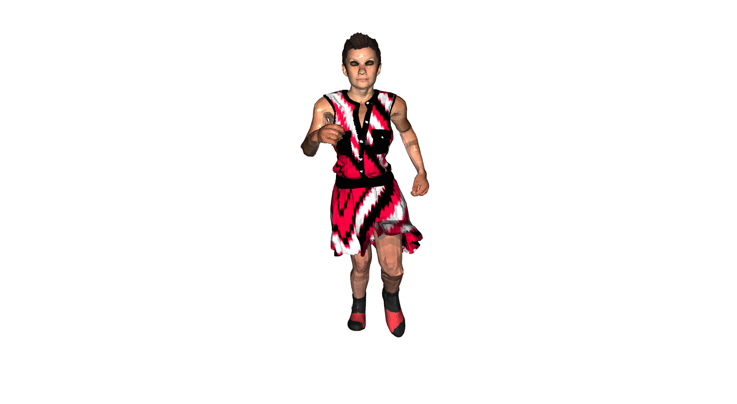
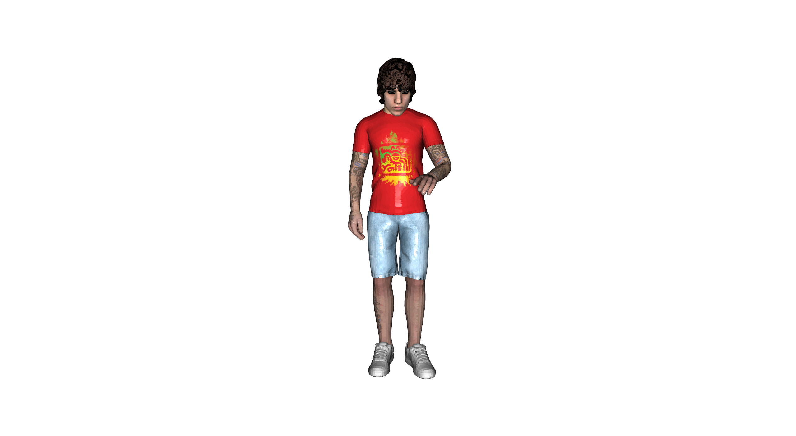
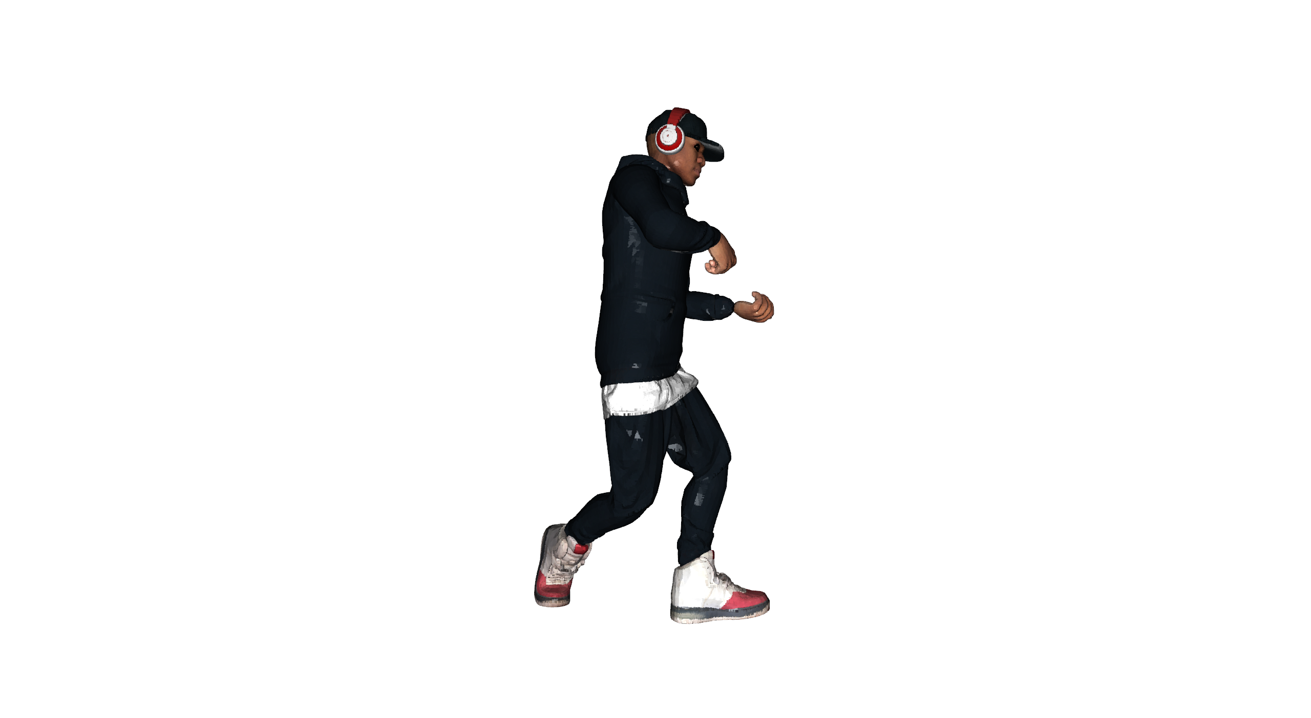
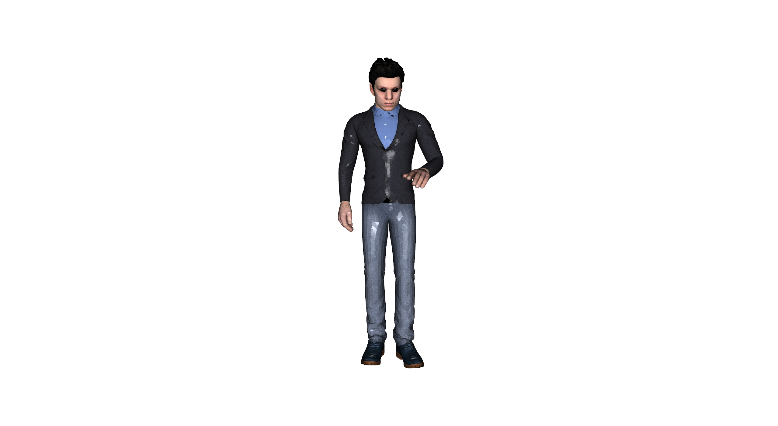
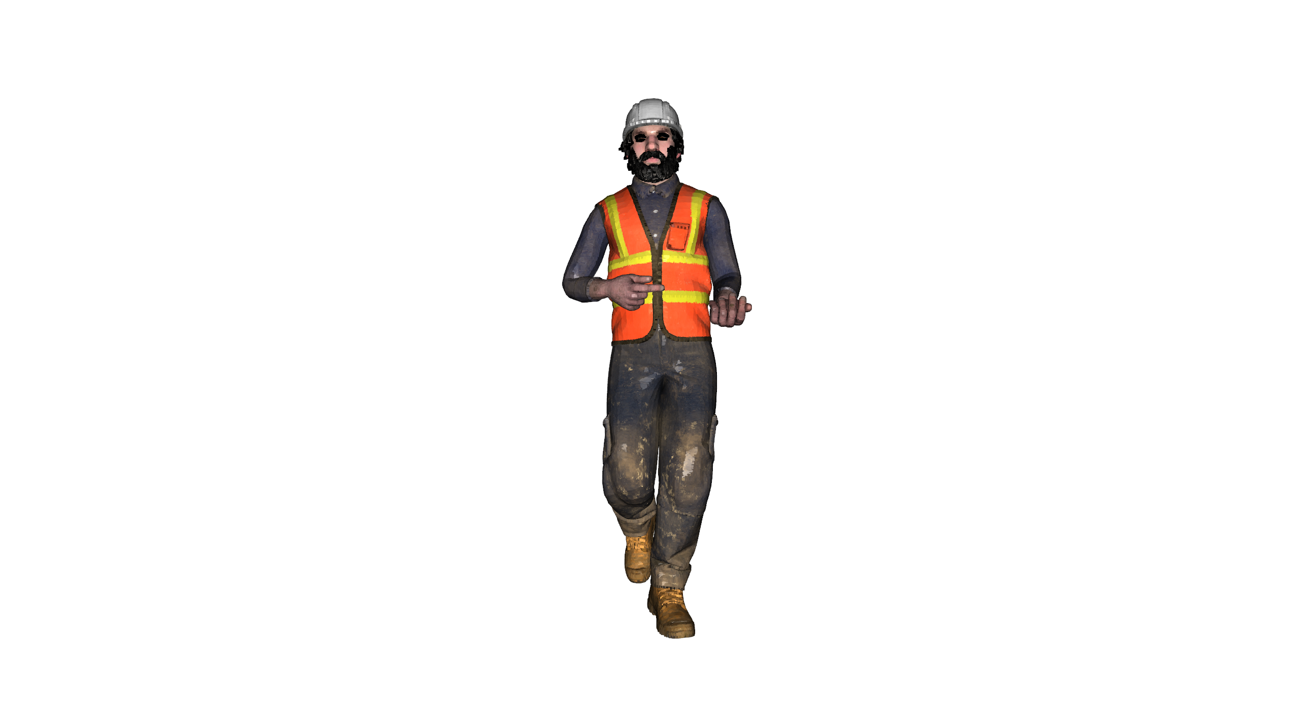
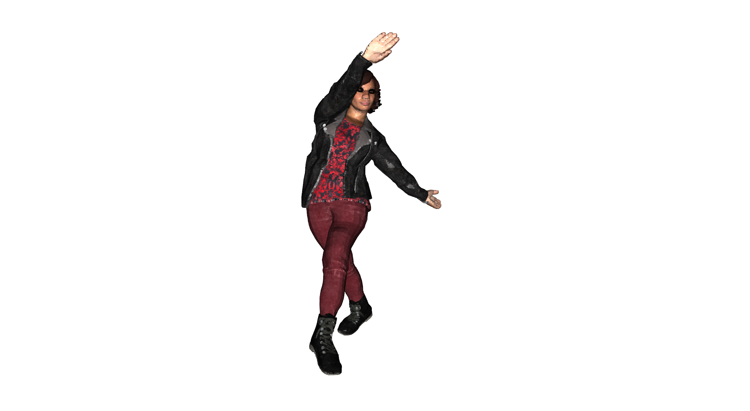
Fig. S1: Test characters: (a) Andromeda (b) Bryce (c) James (d) Pete (f) Shae

B.3 JPEG Pleno 8i Voxelized Full Bodies

The dynamic voxelized point cloud sequences in this dataset are known as the 8i Voxelized Full Bodies (8iVFB). There are four sequences in the dataset, known as longdress, loot, redandblack, and soldier, pictured below. In each sequence, the full body of a human subject is captured by 42 RGB cameras configured in 14 clusters. The point clouds are originally high resolution with over $700,000$ points. The dataset is scaled by a factor of $0.0018$ and subsequently translated $(-0.37426165;-0.03379993;-0.29201281)$ to match the Human Bodies training data scale and general position. The data is then downsampled to 4,000 points using FPS.

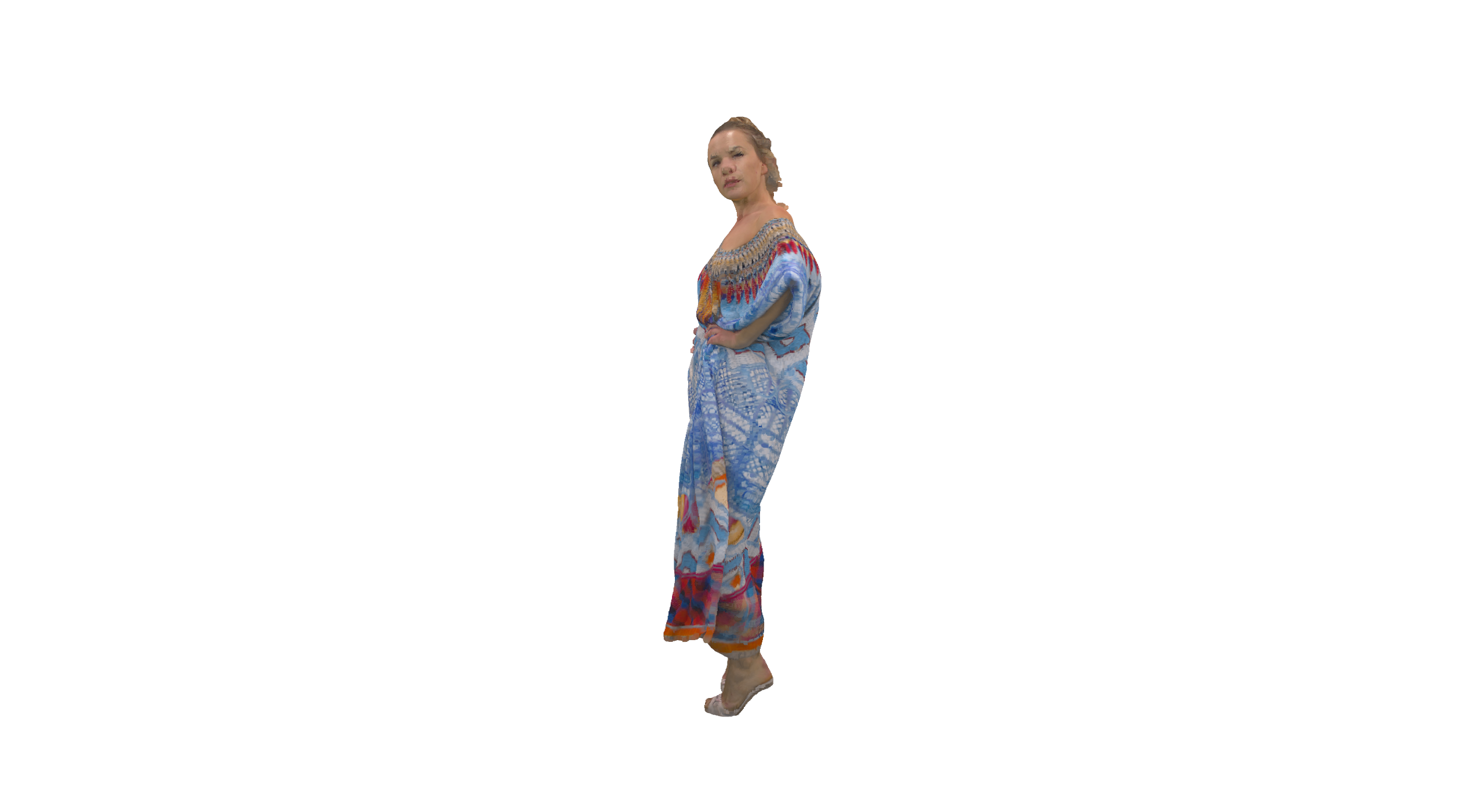
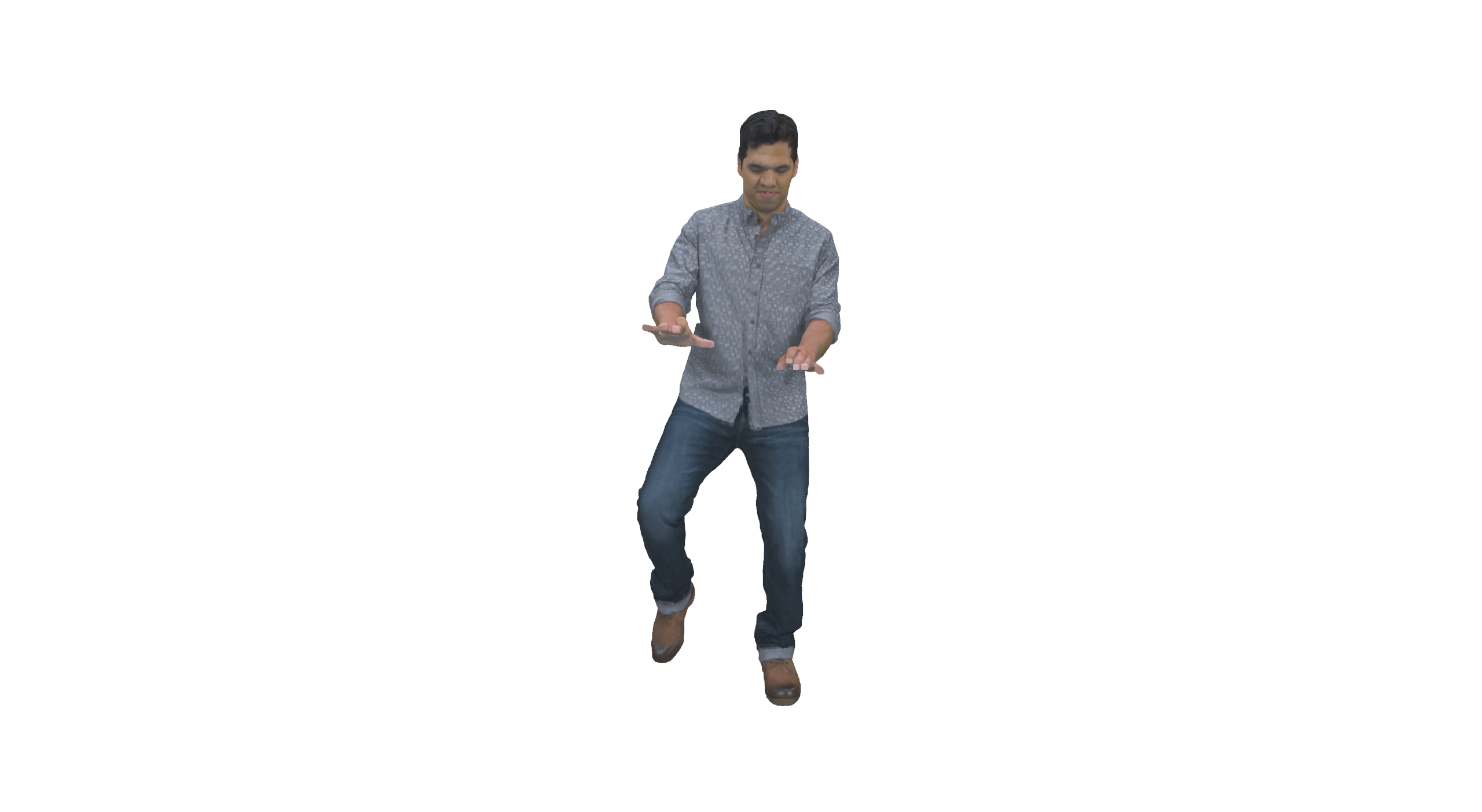
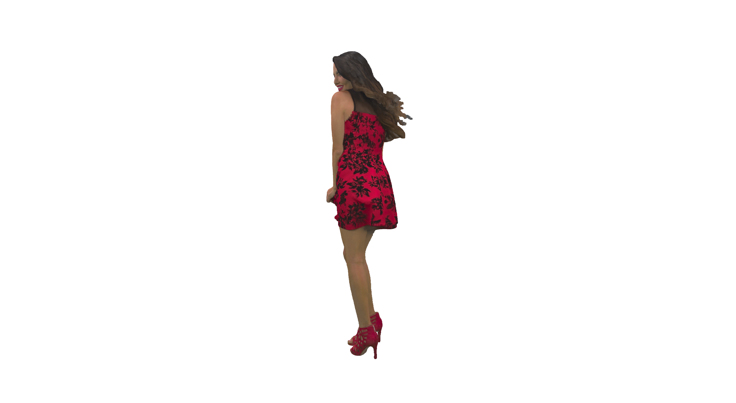
Fig. S2: JPEG Test characters: (a) longdress (b) loot (c) redandblack (d) soldier

FPS was chosen for the last downsample operations because it better coverage of the entire point cloud, compared with random sampling. This dataset is only used for evaluation, of the models trained with the Synthetic Human Bodies dataset.

Appendix C Implementation details

This section describes the parameters and specifications of the proposed framework.

C.1 Training details

The models are trained using the Adam optimizer, with a learning rate of $10^{-5}$ for all datasets. The models trained with the MNIST dataset are trained for $200,000$ interactions with a batch size of 32. For the Synthetic Human Bodies dataset, the PointRNN and Graph-RNN models a batch size of 4 is set and trained for $200,000$ interaction in long-term prediction task and for $150,000$ interaction in short-term prediction task. The Graph-RNN (color) model that considers point clouds with color is trained for $200,000$ interaction for both tasks with a batch size of 2. For all models, the gradients are clipped in range $[5,5]$.

C.2 Architecture Specifications

This section provides the specification for each of the main components: Sampling and Grouping (SG); The Graph neural network (GNN) for features learning; Graph-RNN cells; States propagation (SP); Final Fully connected layer (FC);

The Graph-RNN model is implemented the same way for the MNIST dataset and the Synthetic Human Bodies. For the MNIST dataset, we compare Graph-RNN results with the original PointRNN results ($k$-nn Model). However, since the original PointRNN paper [11] did not perform experiments on the Synthetic Human Bodies dataset, we choose the $k$-values and dimensions to adapt the PointRNN framework to the dataset. To have a fair comparison between our proposed Graph-RNN and Point-RNN, we tried to keep the frameworks as similar as possible while preserving the design choices of each one.

The architecture specifications of both Graph-RNN and PointRNN are displayed in Table S1.

Specifications
number of output points		Graph-RNN model			Point-RNN model
hierarchical	basic	Components	k	ouput channels	Components	k	ouput channels
n/2	-	SG	4	-	SG	4	-
n/2	n	GNN layer 1	16	64	-	-	-
n/2	n	GNN layer 2	16	128	-	-	-
n/2	n	GNN layer 3	8	128	-	-	-
n/2	n	Graph-RNN cell 1	8	256	PointRNN cell 1	24	256
n/4	-	SG	4	-	SG	4	-
n/4	n	Graph-RNN cell 2	8	256	PointRNN cell 2	16	256
n/8	-	SG	4	-	SG	4	-
n/8	n	Graph-RNN cell 3	8	256	PointRNN cell 3	8	256
n/4	-	SP 1	-	256	SP 1	-	256
n/2	-	SP 2	-	256	SP 2	-	256
n	-	SP 3	-	256	SP 3	-	256
n	n	FC 1	-	126	FC1	-	128
n	n	FC 2	-	3	FC 2	-	3
-	-	Graph-RNN (color) model			-	-	-
n	n	FC color 1	-	126	-	-	-
n	n	FC color 2	-	3	-	-	-

Table S1: Architecture specifications. Each component is described by tree attributes, i.e number of output points, number of neighborhoods ($k$) and number of output channel.

For all the models, the final fully connected (FC) layer is implemented in fact by two fully connected layers FC1 and FC2. The FC1 and FC2 layers process the states to predict the geometry displacement.

The Graph-RNN (color) model that takes color as input has two additional fully connected layers (FC1 color and FC2 color). Similar to the FC for points, the FC (color) will take the states as input and predict the color displacement. The assumption that the color of the points does not change during the movement, while mostly correct in the case of synthetically generated data, can not be applied in real-world data. The point’s color can change due to lighting conditions, or in extremes cases, scene objects can transform, or be replaced by new ones. The color prediction was not a priority in this work. The FC (color) does not affect the loss function and has no impact on the overall method. Nevertheless, in long-term prediction evaluation, we disregard the prediction of color displacement and consider instead a null color displacement, meaning all the points keep the same color from frame to frame. In the future, we intend to explore color prediction, by including a color evaluation metric in the loss function.

Appendix D Extra Results visualization

This section presents visualization examples of prediction on Synthetic Human Bodies and JPEG datasets. Long-term prediction examples are depicted on the right side of the next page and short-term prediction examples on left.

Long-term prediction is a very challenging task. In the MNIST dataset, the moving digits perform simple translation movements. The Graph-RNN can effectively model these simple motions over a long period, and make a long-term prediction (10 frames). On the other hand, Synthetic Human Bodies perform more complex activities (e.g dancing, climbing, running). Since these activities are composed of irregular movements, with sudden motion changes, they are incredibly difficult to predict in the long-term.

Figure S3 and Figure S4, show the difficulty in long-term prediction in human activities. Both the PointRNN and Graph-RNN have trouble at preserving the spatial structure over time. This was expected since in long-term prediction the error in each predicted frame is propagated and amplified for each subsequent prediction. While from Figures S3 and S4, it would appear the PointRNN is better at preserving the spatial structure, this is because the PointRNN failed to capture the correct motion. The Graph-RNN, on the other hand, correctly captured the general motion, losing however some of the point cloud shape as a result. We can conclude that a better prediction comes with the risk of higher deformation. The Point-RNN achieved a smaller prediction error in the long-term prediction of the Human Bodies dataset, by making more conservative predictions (low movement prediction). In contrast, the Graph-RNN makes more accurate predictions, however in the cases the predicted motion is wrong, the error is amplified, resulting in a worse average performance.

Figure S6 and S7 display short-term prediction examples. All the models show very similar visual results and can make accurate predictions. The Graph-RNN superior performance can be observed in the small details like in the knee and foot of the model.

Figures S5 and S8 show examples on the JPEG Human Bodies dataset. The point clouds sequence from the JPEG dataset has very little movement, confirmed by the good performance of the Copy Last Input model in both short and long-term prediction. While the Graph-RNN achieved a smaller prediction error in the chosen evaluation metrics, it is difficult to see the performance gains by looking at the prediction visualizations.

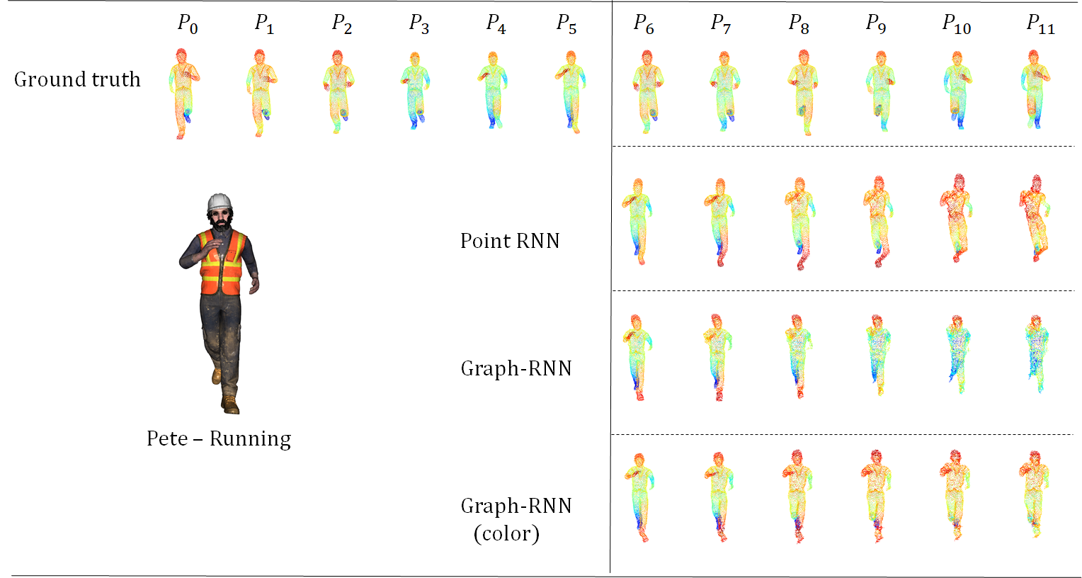
Fig. S3: Short-term prediction on ’Pete Running’ sequence

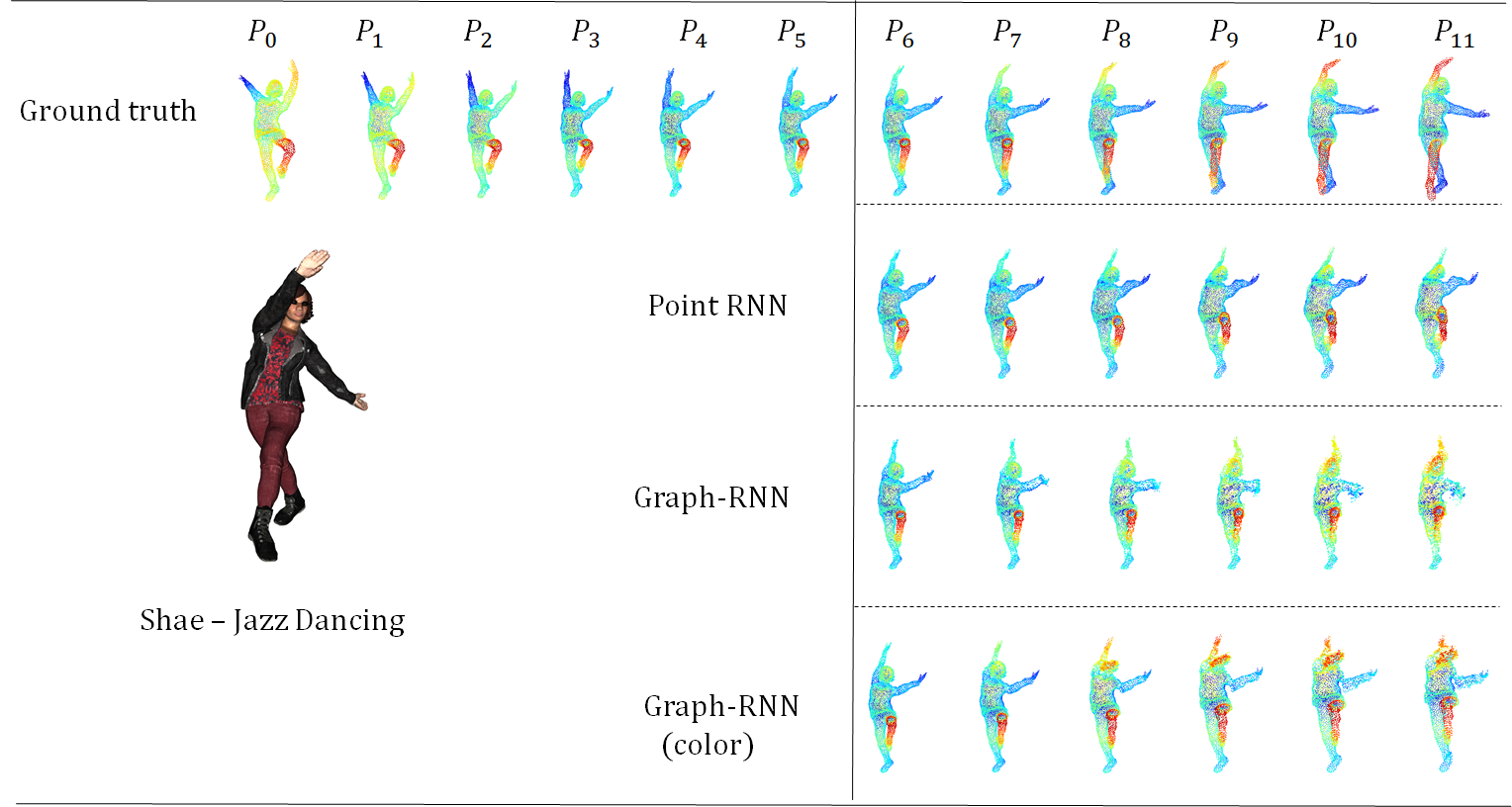
Fig. S4: Short-term prediction on ’Shae Jazz Dancing’ sequence

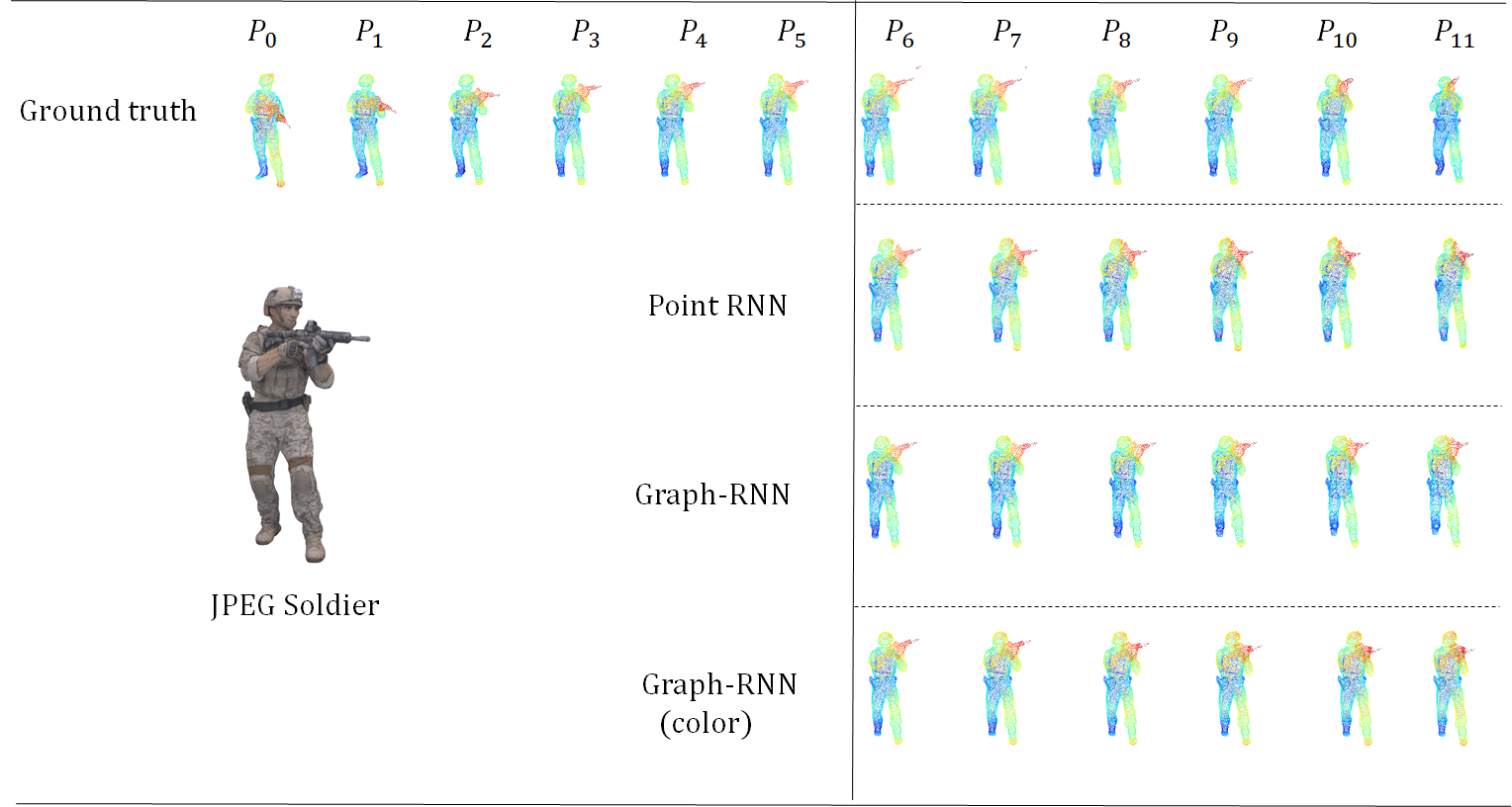
Fig. S5: Short-term prediction on ’JPEG Soldier’ sequence

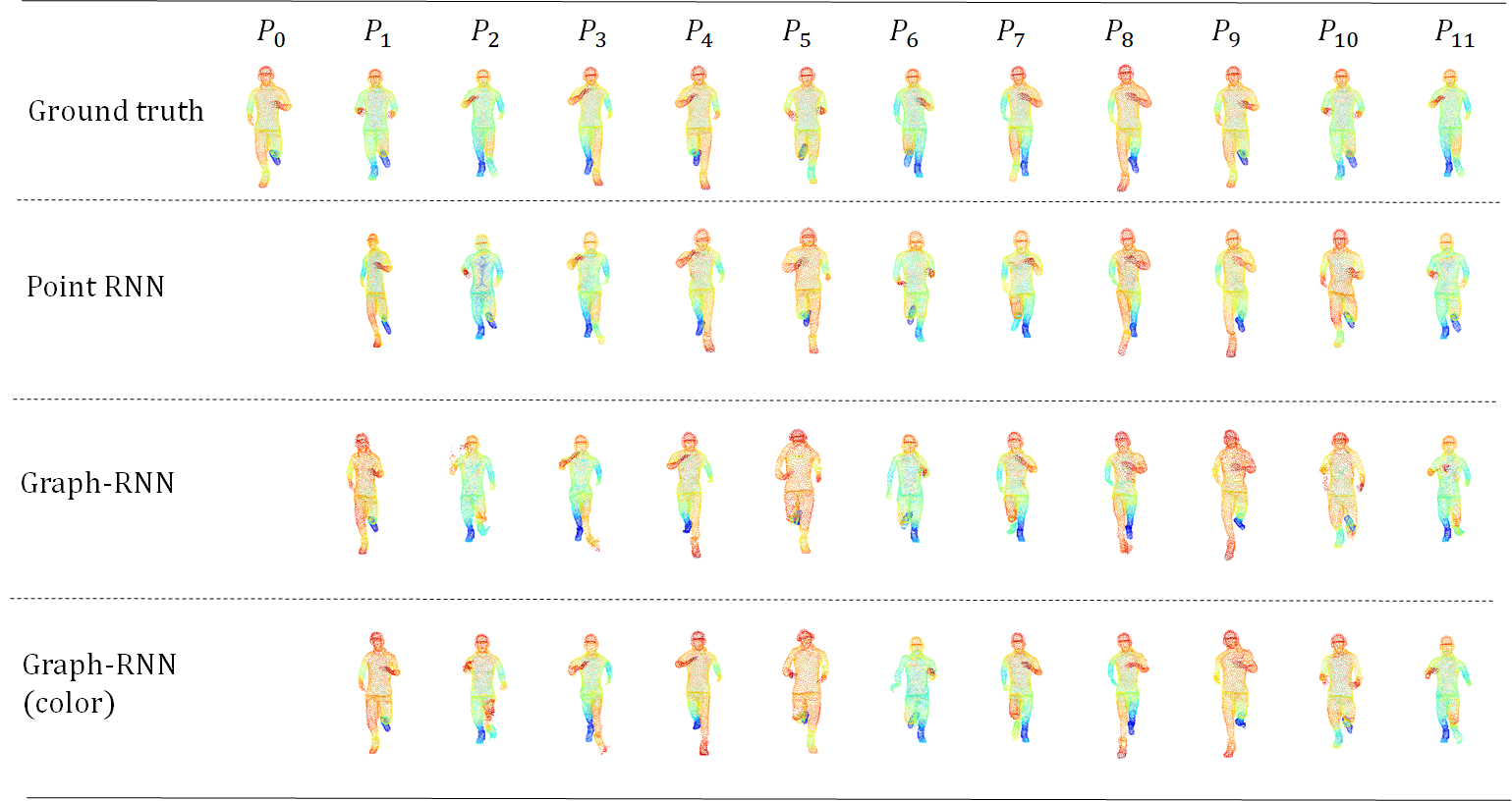
Fig. S6: Short-term prediction on ’James Running’ sequence

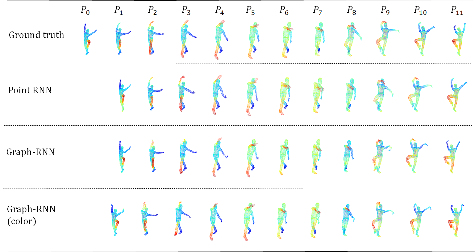
Fig. S7: Short-term prediction on ’Josh Jazz Dancing’ sequence

Fig. S8: Short-term prediction on ’JPEG Redandblackdress” sequence

References

- [1] H. Caesar, V. Bankiti, A. H. Lang, S. Vora, V. E. Liong, Q. Xu, A. Krishnan, Y. Pan, G. Baldan, and O. Beijbom, “nuSscenes: A multimodal dataset for autonomous driving,” in Proc. IEEE/CVF Conf. on Computer Vision and Pattern Recogn., 2020.
- [2] “The BossHoss Augmented Reality,” [Online] Avaliable: https://volucap.de/portfolio-items/the-bosshoss-augmented-reality.
- [3] “Culture 3D Cloud,” [Online] Avaliable: http://c3dc.fr.
- [4] “MPEG 3DG, V-PCC test model v8,” in ISO/IEC JTC1/SC29/WG11N18884, 2019.
- [5] R. Mekuria, K. Blom, and P. Cesar, “Design, implementation, and evaluation of a point cloud codec for tele-immersive Video,” IEEE Trans. Circuits Syst. Video Technol., vol. 27, no. 4, pp. 828–842, 2016.
- [6] R. L. de Queiroz and P. A. Chou, “Motion-compensated compression of point cloud video,” in Proc. IEEE Int. Conf. on Image Processing, 2017.
- [7] D. Thanou, P. A. Chou, and P. Frossard, “Graph-based compression of dynamic 3D point cloud sequences,” IEEE Trans. Image Processing, vol. 25, no. 4, pp. 1765–1778, 2016.
- [8] C. R. Qi, H. Su, K. Mo, and L. J. Guibas, “PointNet: Deep learning on point sets for 3D classification and segmentation,” in Proc. IEEE/CVF Conf. on Computer Vision and Pattern Recogn., 2017.
- [9] G. Zhang, M. Fiore, I. Murray, and P. Patras, “CloudLSTM: A recurrent neural model for spatiotemporal point-cloud stream forecasting,” arXiv preprint arXiv:1907.12410, 2019.
- [10] Y. Min, Y. Zhang, X. Chai, and X. Chen, “An efficient PointLSTM for point clouds based gesture recognition,” in Proc. IEEE/CVF Conf. on Computer Vision and Pattern Recogn., 2020, pp. 5760–5769.
- [11] H. Fan and Y. Yang, “PointRNN: Point recurrent neural network for moving point cloud processing,” arXiv:1910.08287, 2019.
- [12] Y. Wang, Y. Sun, Z. Liu, S. E. Sarma, M. M. Bronstein, and J. M. Solomon, “Dynamic graph CNN for learning on point clouds,” ACM Trans. On Graphics, vol. 38, no. 5, pp. 1–12, 2019.
- [13] F. Pistilli, G. Fracastoro, D. Valsesia, and E. Magli, “Learning robust graph-convolutional representations for point cloud denoising,” IEEE J. Select. Topics in Signal Processing, pp. 1–1, 2020.
- [14] Y. Zhang and M. Rabbat, “A graph-CNN for 3D point cloud classification,” in Proc. IEEE Int. Conf. on Acoustics, Speech and Signal Processing, 2018.
- [15] I. Viola, J. Mulder, F. De Simone, and P. Cesar, “Temporal interpolation of dynamic digital humans using convolutional neural networks,” in Proc. IEEE Int. Conf. on Artificial Intelligence and Virtual Reality, 2019.
- [16] E. d’Eon, B. Harrison, T. Myers, and P. A. Chou, “8i Voxelized Full Bodies A Voxelized Point Cloud Dataset,” ISO/IEC JTC1/SC29 Joint WG11/WG1 (MPEG/JPEG) input document WG11M40059/WG1M74006, Geneva, January 2017.
- [17] C. R. Qi, L. Yi, H. Su, and L. J. Guibas, “PointNet++: Deep hierarchical feature learning on point sets in a metric space,” in Proc. Conf. and Workshop on Neural Information Processing Systems, 2017.
- [18] D.Urbach, Y. Ben-Shabat, and M. Lindenbaum, “DPDist: Comparing point clouds using deep point cloud distance,” arXiv:2004.11784, 2020.
- [19] “Mixamo,” [Online] Avaliable: http://mixamo.com.
- [20] Blender Online Community, Blender - a 3D modelling and rendering package, Blender Foundation, Blender Institute, Amsterdam,
- [21] M. A. Irfan and E. Magli, “3D point cloud denoising using a joint geometry and color k-NN graph,” in Proc. IEEE European Signal Processing Conf., 2021.