Why are ELEvoHI CME arrival predictions different if based on STEREO-A or STEREO-B heliospheric imager observations?
Abstract
Accurate forecasting of the arrival time and arrival speed of coronal mass ejections (CMEs) is a unsolved problem in space weather research. In this study, a comparison of the predicted arrival times and speeds for each CME based, independently, on the inputs from the two STEREO vantage points is carried out. We perform hindcasts using ELlipse Evolution model based on Heliospheric Imager observations (ELEvoHI) ensemble modelling. An estimate of the ambient solar wind conditions is obtained by the Wang-Sheeley-Arge/Heliospheric Upwind eXtrapolation (WSA/HUX) model combination that serves as input to ELEvoHI. We carefully select 12 CMEs between February 2010 and July 2012 that show clear signatures in both STEREO-A and STEREO-B HI time-elongation maps, that propagate close to the ecliptic plane, and that have corresponding in situ signatures at Earth. We find a mean arrival time difference of 6.5 hrs between predictions from the two different viewpoints, which can reach up to 9.5 hrs for individual CMEs, while the mean arrival speed difference is 63 km s-1. An ambient solar wind with a large speed variance leads to larger differences in the STEREO-A and STEREO-B CME arrival time predictions (). Additionally, we compare the predicted arrivals, from both spacecraft, to the actual in situ arrivals at Earth and find a mean absolute error of 7.5 9.5 hrs for the arrival time and 87 111 km s-1 for the arrival speed. There is no tendency for one spacecraft to provide more accurate arrival predictions than the other.
Space Weather
Space Research Institute, Austrian Academy of Sciences, Schmiedlstraße 6, 8042 Graz, Austria University of Graz, Institute of Physics, Universitätsplatz 5, 8010 Graz, Austria Institute of Geodesy, Graz University of Technology, Steyrergasse 30, 8010 Graz, Austria Conrad Observatory, Zentralanstalt für Meteorologie und Geodynamik, Vienna, Austria RAL Space, Rutherford Appleton Laboratory, Harwell Campus, Didcot OX11 0QX, UK Department of Meteorology, University of Reading, Reading, UK
Jürgen Hinterreiterjuergen.hinterreiter@oeaw.ac.at
A comparison of CME arrival time and speed predictions from two vantage points was carried out using ELEvoHI
A highly structured ambient solar wind flow leads to larger arrival time differences between STA and STB predictions
The assumption of a rigid CME front in ELEvoHI and other HI-based methods is most probably too simplistic
1 Introduction
Understanding the dynamics of coronal mass ejections (CMEs) in the heliosphere is a key aspect of space weather research. CMEs are huge clouds of energetic and magnetized plasma (Hundhausen \BOthers., \APACyear1994) erupting from the solar corona that may reach speeds of up to 3000 km s-1. When they hit Earth, CMEs can produce strong geomagnetic storms (Gosling \BOthers., \APACyear1990; Srivastava \BBA Venkatakrishnan, \APACyear2004; Richardson \BBA Cane, \APACyear2012; Kilpua \BOthers., \APACyear2012) causing communication and navigation system problems, damaging satellites and can even cause power outages (Cannon, \APACyear2013). The need for accurate predictions of CMEs, both CME arrival time and speed, is becoming increasingly important (Owens \BOthers., \APACyear2020), because humankind, more than ever, depends on advanced technology.
Shortly after their eruption, CMEs can be observed in coronagraph images. Two of the few space-borne coronagraphs in operation are the Large Angle and Spectrometric Coronagraph (LASCO) C2 and C3 on-board the Solar and Heliospheric Observatory (SoHO; Brueckner \BOthers., \APACyear1995). SoHO is situated in a Lissajous orbit around Lagrange point 1 (L1), about 1.5 million km upstream of Earth in the Sun-Earth line.
The launch of the Solar Terrestrial Relations Observatory (STEREO; Kaiser \BOthers., \APACyear2008) twin-spacecraft mission in 2006 provided an unprecedented opportunity to observe CMEs from off the Sun-Earth line. The two spacecraft orbit the Sun slightly closer (STEREO Ahead; STA) and slightly further (STEREO Behind; STB) than Earth, leading to a separation of each spacecraft by about 22° per year from Earth in opposite directions. Both spacecraft are equipped with the In-situ Measurements of Particles and CME Transients (IMPACT; Luhmann \BOthers., \APACyear2008) instrument package to measure solar wind speed, density and magnetic field and additionally host a suite of imagers, such as the COR1 and COR2 (Howard \BOthers., \APACyear2008) coronagraphs and the heliospheric imagers, HI1 and HI2 (Eyles \BOthers., \APACyear2009). The wide-angle HI cameras provide observations of the heliosphere that allow us to track a CME from close to the Sun out to the orbit of Earth, particularly in the ecliptic plane.
CMEs are optically thin structures that expand rapidly, and decreasing density lowers the line-of-sight integrated intensity in white-light data. As a consequence, the tracking of CME fronts and the interpretation of HI image data is difficult. Furthermore, the plane-of-sky assumption is not valid, and we must assume a certain longitudinal extent of the CME frontal shape.
CMEs may be influenced by different phenomena in the heliosphere, e.g. magnetic forces close to the Sun, high-speed solar wind streams, or by other CMEs (Lugaz \BOthers., \APACyear2012; Kay \BBA Opher, \APACyear2015; Möstl \BOthers., \APACyear2015). The ambient solar wind can also affect the kinematic and morphological characteristics of CMEs (e.g. Gosling \BOthers., \APACyear1990; Gopalswamy \BOthers., \APACyear2000; Manoharan \BOthers., \APACyear2004). A CME originating at a speed much faster than the ambient solar wind speed is likely to experience deceleration while slow CMEs may accelerate during their propagation (Richardson \BBA Cane, \APACyear2010; Manoharan \BBA Mujiber Rahman, \APACyear2011). Hence, not only the propagation direction but also the kinematics and shape of CMEs can be altered (e.g. Savani \BOthers., \APACyear2010; Zuccarello \BOthers., \APACyear2012; Y\BPBID. Liu \BOthers., \APACyear2014; Rollett \BOthers., \APACyear2014; Ruffenach \BOthers., \APACyear2015; Kay \BBA Nieves-Chinchilla, \APACyear2020). By tracking CMEs far out in the heliosphere, we get an understanding of their interaction with the ambient solar wind and co-rotating interaction regions.
Over the last decades, a vast number of CME prediction models have been developed. They include empirical models, e.g. Effective Acceleration Model (EAM; Paouris \BBA Mavromichalaki, \APACyear2017), which use relationships between observable parameters and the transit time. There are also drag-based models, (e.g. DBM; Vršnak \BOthers. \APACyear2013, DBEM; Dumbović \BOthers. \APACyear2018, ANTEATR; Kay \BOthers. \APACyear2020), that make use of physics-based equations and account for drag between the ambient solar wind and the CME. Other models make use of HI images, which require techniques to convert the measured elongation into radial distance. For example, the fixed phi fitting (FPF; Sheeley \BOthers., \APACyear1999; Rouillard \BOthers., \APACyear2008) technique considers a CME as a single point, propagating at a constant speed, and provides an estimate of the constant direction of the CME propagation relative to the observer from the apparent acceleration within a sequence of HI images. The harmonic mean fitting (HMF; Lugaz, \APACyear2010; Möstl \BOthers., \APACyear2011) method is similar except that it describes a CME as a circle that remains attached to the Sun-center. The self-similar-expansion fitting (SSEF; Lugaz \BOthers., \APACyear2010; Davies \BOthers., \APACyear2012; Möstl \BBA Davies, \APACyear2013) technique describes a CME as a circle having an increasing radius as it propagates away from the Sun in such a way that it maintains a constant angular width. FPF and HMF are extremes of the SSEF technique with a half width of 0° and 90°, respectively. More sophisticated models combine both the drag-based approach and HI observations (e.g. DBM fitting; Žic \BOthers. \APACyear2015, Ellipse Evolution model based on HI observations, ELEvoHI; Rollett \BOthers. \APACyear2016; Amerstorfer \BOthers. \APACyear2018). Finally, numerical models, which are computational heavy, solve magnetohydrodynamic (MHD) equations (e.g., ENLIL; Odstrcil \BOthers. \APACyear2004, EUHFORIA; Pomoell \BBA Poedts \APACyear2018) simulating the ambient solar wind in the full heliosphere based on synoptic photospheric magnetic-field maps. CMEs are then injected into these models to provide predictions regarding the arrival time and arrival speed at different locations in the heliosphere.
As noted above, ELEvoHI aims to predict the arrival time and arrival speed of CMEs. The model assumes an elliptical shape for the CME front and incorporates the drag exerted by the ambient solar wind. Also, different sources of ambient solar wind speed (e.g. provided by numerical models) can serve as input to ELEvoHI (Amerstorfer \BOthers., \APACyear2021). In its latest version, the model can be used with STEREO-A HI beacon mode data to provide near real-time CME arrival predictions.
This study assesses ELEvoHI to evaluate arrival time and speed predictions of past CMEs using STEREO HI science-quality data. We perform ELEvoHI ensemble predictions for 12 CMEs, where each CME is modeled using input data from STA and STB, separately. In an idealized case, in which a CME with an elliptical front propagates in an ambient solar wind that is constant in space and time, one would expect to get similar results for the arrival time and arrival speed from the two different vantage points. Instead of inferring the propagation directions of the events under study from HI images (e.g. FPF, SSEF), as was done by Amerstorfer \BOthers. (\APACyear2018), we make use of coronagraph images and perform Graduated Cylindrical Shell (GCS; A\BPBIF\BPBIR. Thernisien \BOthers., \APACyear2006; A. Thernisien \BOthers., \APACyear2009) reconstruction for each CME based on multi-vantage point coronagraph data. Additionally, we apply a combination of the Wang-Sheeley-Arge (Arge \BOthers., \APACyear2003) and the Heliospheric Upwind eXtrapolation (Riley \BBA Lionello, \APACyear2011; Owens \BBA Riley, \APACyear2017) model (WSA/HUX model combination; Reiss \BOthers., \APACyear2019, \APACyear2020) to get an estimate of the ambient solar wind conditions in the heliosphere through which the CME propagates. With the additional information about the propagation direction of the CME and the modeled ambient solar wind, ELEvoHI is more likely to give better arrival time and arrival speed predictions.
In Section 2, we describe our data selection process, including the data products, and list all of the studied CMEs. Section 3 deals with the ELEvoHI setup and how the input data required by the model is obtained. In Section 4, we present our results and give reasons for the difference in the model predictions based on STA and STB input data. The discussion and further implementations of the model are included in Section 5.
2 Data Preparation
| Nr. | ID STA | Date STA | ID STB | Date STB | ICMECAT ID | ICME date | |
| [km s-1] | |||||||
| 1 | HCME_A__ 20100203_01 | 2010-02-03 14:49 | HCME_B__ 20100203_01 | 2010-02-03 20:49 | ICME_Wind_ NASA_20100207_01 | 2010-02-07 18:04b) | 4062 |
| \hdashline2 | HCME_A__ 20100319_01 | 2010-03-19 22:09 | HCME_B__ 20100319_01 | 2010-03-19 20:09 | ICME_Wind_ MOESTL_20100323_01 | 2010-03-23 22:29c) | 29212 |
| \hdashline3 | HCME_A__ 20100403_01 | 2010-04-03 12:09 | HCME_B__ 20100403_01 | 2010-04-03 12:09 | ICME_Wind_ NASA_20100405_01 | 2010-04-05 07:55a) | 73418 |
| \hdashline4 | HCME_A__ 20100408_01 | 2010-04-08 06:49 | HCME_B__ 20100408_01 | 2010-04-08 07:29 | ICME_Wind_ NASA_20100411_01 | 2010-04-11 12:20a) | 43217 |
| \hdashline5 | HCME_A__ 20100523_01 | 2010-05-23 22:09 | HCME_B__ 20100524_01 | 2010-05-24 00:09 | ICME_Wind_ NASA_20100528_01 | 2010-05-28 01:52a) | 37010 |
| \hdashline6 | HCME_A__ 20101026_01 | 2010-10-26 15:29 | HCME_B__ 20101026_01 | 2010-10-26 16:10 | ICME_Wind_ MOESTL_20101030_01 | 2010-10-30 09:15b) | 3809 |
| \hdashline7 | HCME_A__ 20110130_01 | 2011-01-30 20:09 | HCME_B__ 20110130_01 | 2011-01-30 18:49 | ICME_Wind_ MOESTL_20110204_01 | 2011-02-04 01:50a) | 3759 |
| \hdashline8 | HCME_A__ 20110214_02 | 2011-02-14 22:49 | HCME_B__ 20110214_02 | 2011-02-14 22:09 | ICME_Wind_ MOESTL_20110218_01 | 2011-02-18 00:48a) | 49325 |
| \hdashline9 | HCME_A__ 20110906_02 | 2011-09-06 23:29 | HCME_B__ 20110907_01 | 2011-09-07 03:29 | ICME_Wind_ MOESTL_20110909_01 | 2011-09-09 11:46a) | 41720 |
| \hdashline10 | HCME_A__ 20120123_01 | 2012-01-23 04:49 | HCME_B__ 20120123_01 | 2012-01-23 05:29 | ICME_Wind_ MOESTL_20120124_01 | 2012-01-24 14:36a) | 61336 |
| \hdashline11 | HCME_A__ 20120614_01 | 2012-06-14 16:09 | HCME_B__ 20120614_01 | 2012-06-14 16:09 | ICME_Wind_ MOESTL_20120616_01 | 2012-06-16 19:34a) | 48929 |
| \hdashline12 | HCME_A__ 20120712_02 | 2012-07-12 18:49 | HCME_B__ 20120712_01 | 2012-07-12 18:09 | ICME_Wind_ MOESTL_20120714_01 | 2012-07-14 17:38a) | 61537 |
-
a)
shock arrival time
-
b)
time of density enhancement
-
c)
time of the magnetic flux rope
We select a period between February 2010 and July 2012 during which the STEREO spacecraft had a separation angle from Earth of about 65° to 120° respectively, from which we study 12 CMEs. The HELCATS HICAT CME catalog lists about 700 entries over this time range (Harrison \BOthers., \APACyear2018). However, our list is constrained to 12 events, since the CMEs have to:
-
1)
be observed by HI on both STA and STB spacecraft (as listed in the HIJoinCAT; Barnes2020)
-
2)
propagate close to the ecliptic plane,
-
3)
have a corresponding in situ signature at Earth,
-
4)
be able to be tracked unambiguously in time-elongation maps.
Table 1 contains the list of selected CMEs with their unique identifier and the time of their first observation in HI1 images (according to the HELCATS catalog Version 6). The interplanetary CME (ICME) times and speeds are taken from version 2.0 of the HELCATS ICMECAT catalog (Möstl \BOthers., \APACyear2020, see also the links in the data section). The ICMECAT assimilates ICME catalogs from different spacecraft into one consistent list, and was first published in Möstl \BOthers. (\APACyear2017). The ICME date as observed by the Wind spacecraft is defined by the shock arrival time, or, if no shock is present, the start of a density enhancement in front of the magnetic flux rope (MFR). If neither is observed, the ICME start time is taken as the start time of the MFR. The corresponding ICME speed is the mean proton bulk speed of either the sheath region, the density enhancement ahead of the MFR, or the speed of the MFR itself. The spread in the speed over the given interval for each event is indicated in Table 1 by a standard deviation. For Table 1, some times in the ICMECAT were originally taken from the Wind ICME catalog (Nieves-Chinchilla \BOthers., \APACyear2018), while other events that were not present in the Wind catalog were added by Möstl \BOthers. (\APACyear2020) to the HELCATS ICMECAT.
To run ELEvoHI, we make use of several data products. Most important are images from HI onboard STEREO. The HI instrument on each STEREO spacecraft consists of two white-light wide-angle imagers, HI1 and HI2. HI1 has a field-of-view (FOV) extending from 4° – 24° elongation (angle from Sun center) in the ecliptic and HI2 has an angular FOV extending from 18.8° – 88.8° elongation in the ecliptic. The nominal cadence of the HI1 and HI2 science data is 40 minutes and 120 minutes, respectively. The science image bin size is 70 arc sec for HI1 and 4 arc min for HI2. For the additional input parameters to ELEvoHI, we developed the Ecliptic cut Angles from GCS for ELEvoHI tool (EAGEL, see Section 3.1). EAGEL ideally uses coronagraph images from STEREO COR1/COR2 and from LASCO C2/C3 onboard SoHO, but images from at least two different viewpoints are required. The FOV of COR1 ranges from 1.4 – 4 R⊙ and COR2, from 2 – 15 R⊙, while C2 has a FOV of 1.5 – 6 R⊙ and C3, 3.7 – 30 R⊙ (all quoted in the plane-of-sky). The cadence of the coronagraph science images is about 15 minutes.
3 Methods
3.1 EAGEL (Ecliptic cut Angles from GCS for ELEvoHI)
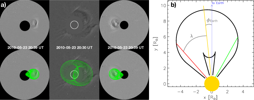
In this section, we present a newly developed Interactive Data Language (IDLTM) tool called EAGEL (Ecliptic cut Angles from GCS for ELEvoHI). EAGEL allows the user to determine the propagation direction, , and the half width, , within the ecliptic plane, based on GCS reconstruction of a CME. To perform GCS reconstruction, coronagraph images from at least two vantage points (STEREO and/or LASCO) are required. EAGEL provides the routines to download the required coronagraph images, combines all the functions to perform GCS reconstruction, and produces a cut in the ecliptic plane. Standard pre-processing of the images is implemented in EAGEL to make the CME features clearly visible to the user, who can decide between using background-subtracted, running-difference, and base-difference images. The user can then perform GCS reconstruction using the IDL SolarSoft procedure rtsccguicloud. The top row of Figure 1a shows the coronagraph images (from left to right: STB/COR2, LASCO/C2, STA/COR2) for event 5. The bottom row additionally shows the GCS wire frame (green mesh). In its current version, ELEvoHI is a 2D prediction model giving results only in the ecliptic plane. Therefore, EAGEL calculates the ecliptic part of the GCS wire frame and selects the boundaries of the ecliptic cut (see red and green line in Figure 1b). The boundaries are defined to be the outermost points of each side of the ecliptic cut with respect to the apex direction from GCS reconstruction. This gives and , where the latter is defined to be exactly in between the two boundaries. A plot is shown to the user (Figure 1b) and, if needed, the boundaries can be changed manually. Once the user approves the selection, and relative to Earth and to the two STEREO spacecraft are stored and can be used by ELEvoHI.
In Table 2, we list the time (Date) of the STEREO coronagraph images used to get and for each event. EAGEL then selects the SoHO coronagraph images closest in time to the quoted date. Each CME is fitted once based on the three different viewpoints (STA, STB, LASCO). However, for event 1 no LASCO data is available, so GCS reconstruction is based on STEREO images only. For all the events, the times of the images are selected in such a way that the CME front is clearly visible in the coronagraph images of all the viewpoints. Furthermore, we try to fit the CME at times when the front is already far out in both STA and STB COR2 images. Table 2 additionally contains the GCS parameters (Lon, Lat, TA, AR, HA). Also the half width, , and the CME ecliptic propagation angle, , relative to Earth () and relative to the two STEREO spacecraft ( and ) obtained from EAGEL are given. Lon is the longitude (here given in Stonyhurst coordinates) and Lat the latitude of the apex of the idealized hollow croissant shaped model. The tilt angle (TA) defines the tilt of the croissant, calculated with respect to the solar equator. The half angle (HA) represents the angle between the center of the footpoints and the aspect ratio (AR) is the ratio of the CME size in two orthogonal directions.
When comparing (longitude from GCS reconstruction) and (longitude relative to Earth from the ecliptic cut), it can be seen that the propagation direction obtained from the ecliptic cut is quite comparable to (within 5° of) the propagation direction from the GCS reconstruction. Only for events 6 and 10 we find differences of about 30° and 10°, respectively. The reason can be found in the combination of low/high latitude and large tilt angle. Therefore, the part within the ecliptic plane does not correspond well to the main propagation direction resulting from GCS reconstruction for these two CMEs.
| GCS parameter | EAGEL results | |||||||||
| Nr. | Date | Lon | Lat | TA | AR | HA | ||||
| [°] | [°] | [°] | [°] | [°] | [°] | [°] | [°] | |||
| 1 | 2010-02-03 15:54 | 355 | -17 | -1 | 0.33 | 30 | 36 | -4 | 67 | 68 |
| 2 | 2010-03-19 17:39 | 23 | -12 | -7 | 0.29 | 19 | 30 | 22 | 44 | 93 |
| 3 | 2010-04-03 12:39 | 7 | -19 | 15 | 0.39 | 30 | 38 | 9 | 58 | 81 |
| 4 | 2010-04-08 06:39 | 1 | -10 | -20 | 0.28 | 30 | 31 | -2 | 70 | 69 |
| 5 | 2010-05-23 20:39 | 6 | 2 | -15 | 0.48 | 18 | 35 | -6 | 65 | 76 |
| 6 | 2010-10-26 14:39 | 18 | -35 | -28 | 0.51 | 30 | 18 | -11 | 95 | 69 |
| 7 | 2011-01-30 21:24 | 351 | -18 | -20 | 0.33 | 12 | 24 | -11 | 97 | 82 |
| 8 | 2011-02-15 04:08 | 10 | -10 | 27 | 0.87 | 29 | 49 | 10 | 77 | 104 |
| 9 | 2011-09-06 23:39 | 29 | 20 | -90 | 0.49 | 30 | 26 | 29 | 74 | 124 |
| 10 | 2012-01-23 04:39 | 19 | 41 | 64 | 0.77 | 55 | 37 | 9 | 99 | 123 |
| 11 | 2012-06-14 14:54 | 360 | -28 | 11 | 0.90 | 30 | 53 | 1 | 116 | 117 |
| 12 | 2012-07-12 17:54 | 8 | -12 | 68 | 0.46 | 30 | 26 | 14 | 106 | 129 |
3.2 WSA/HUX model
In the following paragraph, we summarize the main characteristics of the numerical framework used here for modelling the physical conditions in the evolving ambient solar wind flow. For this study, we make use of the framework shown in Reiss \BOthers. (\APACyear2019, \APACyear2020), but the components of this framework were developed by Y\BHBIM. Wang \BBA Sheeley (\APACyear1995), Arge \BOthers. (\APACyear2003), Riley \BBA Lionello (\APACyear2011), and Owens \BBA Riley (\APACyear2017). Specifically, we use magnetic maps of the photospheric field from Global Oscillation Network Group (GONG) provided by the National Solar Observatory (NSO) as input to magnetic models of the solar corona. Using the Potential Field Source Surface model (PFSS; Altschuler \BBA Newkirk, \APACyear1969; Schatten \BOthers., \APACyear1969) and the Schatten current sheet model (SCS; Schatten, \APACyear1971) we compute the global coronal magnetic field topology. While the PFSS model attempts to find the potential magnetic field solution in the corona with an outer boundary condition that the field is radial at the source surface at 2.5 R⊙, the SCS model in the region between 2.5 and 5 R⊙ accounts for the latitudinal invariance of the radial magnetic field as observed by Ulysses (Y\BHBIM. Wang \BBA Sheeley, \APACyear1995). From the global magnetic field topology, we calculate the solar wind conditions near the Sun using the established Wang-Sheeley-Arge (WSA) model. To map the solar wind solutions from near the Sun to Earth, we use the Heliospheric Upwind eXtrapolation model (HUX). This model simplifies the fluid momentum equation as much as possible, by neglecting the pressure gradient and the gravitation term in the fluid momentum equations as proposed by Riley \BBA Lionello (\APACyear2011). The HUX model solutions match the dynamical evolution explored by global heliospheric MHD codes fairly well while having low processor requirements. An example of the ambient solar wind, modeled by WSA/HUX combination, is shown in Figure 2.
3.3 ELEvoHI ensemble modeling
ELEvoHI uses HI time-elongation profiles of CME fronts and assumes an elliptical shape for those fronts to derive their interplanetary kinematics (detailed information about the underlying Ellipse Conversion method can be found in Rollett \BOthers., \APACyear2016). The tracking of each CME was done manually using ecliptic time-elongation maps (j-maps; Sheeley \BOthers., \APACyear1999; Davies \BOthers., \APACyear2009), generated by extracting ecliptic data from STA and STB HI images. Transients, like CMEs, appear as a bright feature in the j-maps. To extract the time-elongation profiles, we use the SATPLOT tool implemented in IDLTM SolarSoft. It allows any user to measure the elongation, which is defined as the angle between the Sun - observer (STA or STB) line and the CME front. ELEvoHI converts the resulting time-elongation profiles to time-distance profiles, assuming an elliptic frontal shape using the ELEvoHI built-in procedure ELlipse Conversion (ELCon; Rollett \BOthers., \APACyear2016).
ELEvoHI accounts for the effect of the drag force exerted by the ambient solar wind, which is incorporated in the model. The drag force is an essential factor influencing the dynamic evolution of CMEs in the heliosphere. Within ELEvoHI, the time-distance track is fitted using a drag-based equation based on the drag-based model (DBM) given in Vršnak \BOthers. (\APACyear2013). The user has to define the start- and end point for the DBM fit (usually around R⊙) in the time-distance profile. In order to account for the de-/acceleration of the CME due to drag, an estimate of the ambient solar wind speed is needed. Here we make use of the WSA/HUX model (see Section 3.2). It provides the ambient solar wind conditions for a full Carrington rotation (see Figure 2). We only consider the part of the full map according to the start- and end-point selected by the user, and the CME propagation direction and half width from EAGEL. From this area surrounded by the white box in Figure 2, we take the median of the solar wind speed and define the uncertainties to be 100 km s-1, based on a study by Reiss \BOthers. (\APACyear2020). They considered nine years (mid 2006 to mid 2015) and report a mean absolute error of the WSA solar wind speed prediction with respect to the in situ speed of 91 km s-1. The obtained ambient solar wind speed with its uncertainty is split into steps of 25 km s-1, which gives nine different input speeds to ELEvoHI. For each of the nine input speeds DBM fitting is performed. ELEvoHI then selects the combination of drag parameter and ambient solar wind speed that best fits the time-distance profile for each ensemble member (for a detailed description see Rollett \BOthers., \APACyear2016). The selected drag parameter and solar wind speed is assumed to be valid for the full CME front during the propagation in the heliosphere.
Since ELEvoHI is a 2D model, we are only interested in the propagation of a CME in the ecliptic plane. and , in this plane, are provided by EAGEL (see Section 3.1). The inverse ellipse aspect ratio, , defines the shape of the assumed CME front in the ecliptic plane, where represents a circular front, while corresponds to an elliptical CME front (with the semi-major axis perpendicular to the propagation direction)
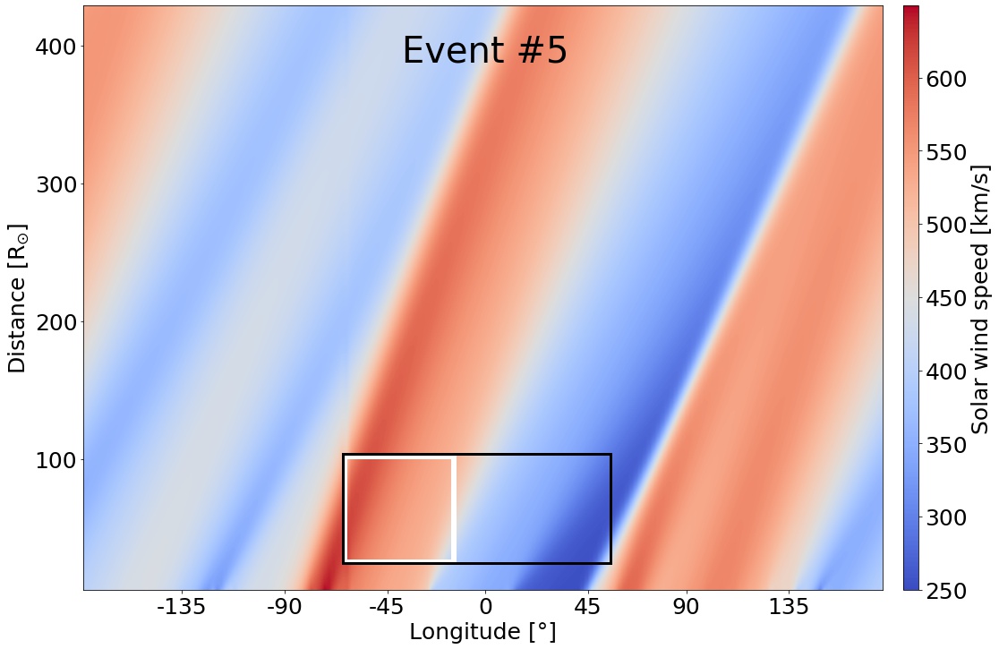
To run ELEvoHI in ensemble mode, we vary , , and . A details description can be found in Amerstorfer \BOthers. (\APACyear2018) and the code is available online (see Section 6). and vary over a range of ° from their values obtained from EAGEL, with a step size of ° and °, respectively. This range is defined based on a study by Mierla \BOthers. (\APACyear2010), who report an uncertainty in the parameters when different users manually perform GCS reconstruction. Note that the propagation direction and the half width obtained from EAGEL are rounded to even numbers and to whole tens, respectively. For we set a fixed range from ( step size). Thus we get a total of 220 ensemble members for one ELEvoHI event (i.e. 11 values of , 5 values of and 4 values of ). For each ensemble member we select a different sector from the ambient solar wind provided by the WSA/HUX model combination according to the propagation direction, half width, start- and end-point. In Figure 2, the WSA/HUX model results for event are shown. The white box indicates the area from which the ambient solar wind speed for one individual run of ELEvoHI is computed. Shown is the area for the minimum propagation direction, of 56° with a of 50°. For each ensemble member the area surrounded by the white box is slightly different according to and . The black box plotted indicates the total area based on all ELEvoHI ensemble members for this event.
Running ELEvoHI in ensemble mode enables us to calculate a mean and a median predicted CME arrival time and also to define an uncertainty. In addition, we can give a probability for whether a CME is likely to hit Earth or not. When all of the 220 ensemble members predict an arrival at Earth, we assume the predicted likelihood of an Earth hit to be 100%.
4 Results
| Nr. | Date STA | SDSTA | Date STB | SDSTB | STA - STB | |||
| [h] | [h] | [h] | [km s-1] | [km s-1] | [km s-1] | |||
| 1 | 2010-02-07 11:24 | 1.5 | 2010-02-07 20:24 | 2.1 | -9.0 | 60 | ||
| \hdashline2 | 2010-03-24 07:17 | 9.1 | 2010-03-24 16:40 | 4.1 | -9.5 | 50 | ||
| \hdashline3 | 2010-04-05 13:23 | 2.5 | 2010-04-05 16:06 | 0.4 | -2.7 | 24 | ||
| \hdashline4 | 2010-04-11 16:07 | 0.6 | 2010-04-12 00:12 | 5.1 | -8.1 | 52 | ||
| \hdashline5 | 2010-05-27 17:36 | 1.9 | 2010-05-28 02:26 | 1.2 | -8.8 | 48 | ||
| \hdashline6 | 2010-10-30 11:24 | 1.4 | 2010-10-30 04:43 | 7.1 | 6.7 | -44 | ||
| \hdashline7 | 2011-02-04 01:08 | 2.4 | 2011-02-03 22:24 | 7.3 | 4.5 | -59 | ||
| \hdashline8 | 2011-02-18 06:22 | 2.8 | 2011-02-18 10:34 | 6.1 | -4.3 | 71 | ||
| \hdashline9 | 2011-09-10 18:55 | 14.9 | 2011-09-10 09:48 | 5.4 | 9.1 | -34 | ||
| \hdashline10 | 2012-01-24 17:49 | 4.0 | 2012-01-24 13:29 | 3.6 | 4.3 | -189 | ||
| \hdashline11 | 2012-06-16 15:47 | 3.8 | 2012-06-16 07:53 | 5.2 | 7.9 | -37 | ||
| \hdashline12 | 2012-07-14 22:16 | 4.9 | 2012-07-14 18:53 | 3.7 | 3.5 | 89 |
We perform ELEvoHI ensemble modeling for 12 CMEs between February 2010 to July 2012 (see Table 1) and compare the predicted arrival times based on STA and STB HI observations with each other. The CMEs propagated close to the ecliptic plane and showed clear in situ signatures at L1. A prerequisite for the chosen CMEs was that the CMEs could be tracked unambiguously in both STA and STB HI j-maps.
In Table 3, we list the predicted ensemble median arrival times and speeds with their standard deviation for each CME under study. It further contains the difference between the predictions from the two vantage points. We find that the predicted arrival times for STA and STB can deviate by up to 9.5 hrs while the mean difference is 6.5 hrs. The mean difference in the arrival speed is 63 km s-1, with an exceptionally large discrepancy of 189 km s-1 for event .
The largest arrival time differences are found for events and . The arrival probability, based on the number of ensemble members that are predicted to hit Earth, is 79% for event and only 56% for event . According to their relatively large angle of propagation with respect to the Sun-Earth line, the CMEs (°, °) and (°, °) are considered as ”flank hits”. In such cases, ELEvoHI tends to predict the CME arrival time to be later than detected in-situ. The reason may be found in the assumed circular CME front for . For future versions of ELEvoHI, we will consider different approaches to tackle such extreme delays for flank encounters e.g. by changing the values for (from 0.4 to 0.7). Braga \BOthers. (\APACyear2020) found a value of for most of the CMEs in their study.
Event 11 occurred on June 14, 2012 and was studied e.g. by Kubicka \BOthers. (\APACyear2016) who report two preceding CMEs. However, the WSA/HUX model does not provide the ambient solar wind conditions with preceding CMEs included and is therefore most probably not suitable for interaction events. The events , , and also show large differences in the predicted arrival times based on STA and STB observations. However, these differences are most certainly related to large variance in the modeled ambient solar wind speeds that are used as input to ELEvoHI (see Section 4.2 and Figure 5 and 6).
4.1 Tracking different parts of the CME front
It is important to keep in mind that different parts of the CME front are tracked in STA and STB HI images. This leads to different input conditions to the ELEvo propagation model for STA and STB. ELEvoHI is designed to take HI tracks for the same CME from different viewpoints. Ideally, predictions should give the same CME speed and direction in both cases. One problem is, however, that the CME is not behaving as a single coherent entity, but is instead moving with different speeds at different longitudes (Owens \BOthers., \APACyear2017), which is not incorporated within ELCon nor in any other HI conversion method (e.g. SSE, FP, and HM).
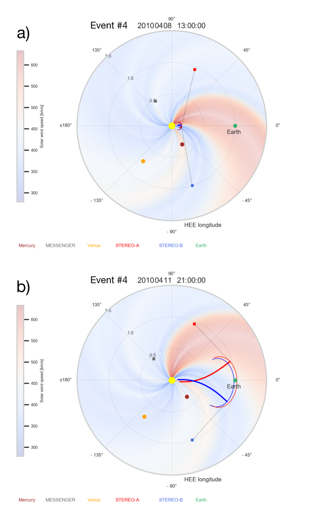
Figure 3 presents two snapshots of a movie for event , with the ambient solar wind provided by WSA/HUX model combination and the positions of various spacecraft and planets. The elliptical CME fronts from one ensemble member based on STA and STB observations are shown in red and blue, respectively. The gray lines from the two STEREO spacecraft to the elliptical CME fronts are plotted. These tangents correspond to the elongations of the leading edge of the CME at these times. At the end of these lines, we add a point, which is the ’tangent point’ at each time step. Over the course of the simulation, these points trace out curved lines, in red and blue for STA and STB, respectively. From Figure 3, it is obvious that, in the near-Sun part of the HI FOV, the observed leading edge is close to the apex of the idealized CME front for both STEREO spacecraft. As the CME propagates, the tangent point, i.e. the part of the CME with the greatest elongation seen by STA and STB progressively moves out to the flanks of the ellipse. Based on the observations of these tangent points, the prediction for the whole front is conducted. Hence, the apex of the CME is, if at all, only observed for a short period of time. In order to get an estimate of the CME Earth arrival we have to assume a designated shape of the CME front, which is in our case, an ellipse. As shown by Owens \BOthers. (\APACyear2017) this assumption might not be valid since the CME interacts with the ambient solar wind.
4.2 Effect of the ambient solar wind
When considering different points along the idealized elliptical CME front, it is noteworthy that the ambient solar wind speeds at these points would likely be different. Furthermore, the part of the CME front corresponding to the greatest elongation as seen by STA and STB (i.e. the points corresponding to the tangent to the CME front) would propagate in different ambient solar wind conditions. In Figure 4, the modeled time-elongation profiles of the tangent points seen from STA (top panel) and STB (bottom panel) for event 4 are shown.
These profiles are obtained from one modeled ensemble member of the ELEvoHI prediction, separately for STA and STB (see Figure 3), and are therefore available from 2010-04-08 11:00 until 2010-04-14 10:00. As long as the CME front could be tracked in HI images (until about 2010-04-10 01:00), the plotted profiles are consistent with the measured HI time-elongation profiles, obtained using the SATPLOT tool. The colors represent the speed of the ambient solar wind at the corresponding points. Due to the propagation of the modeled CME in the heliosphere, the elongation of the tangent point ranges from roughly 8° to about 92° and the speed of the ambient solar wind at these points ranges from 330 km s-1 to 500 km s-1, with a maximum speed of 530 km s-1 at about 66°, for STA (top panel in Figure 4). The range of the elongation is similar for STB (6° to 91°) but the ambient solar wind speed ranges only from 450 km s-1 to 365 km s-1.
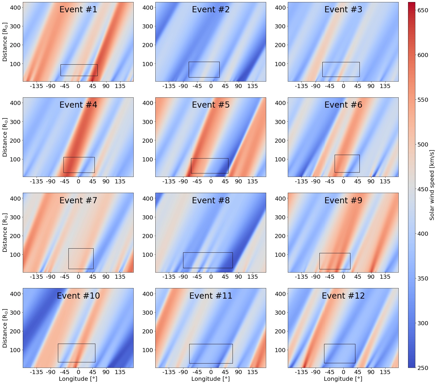
In the previous paragraph, we considered the ambient solar wind speed at the tangent point for one ensemble member. Additionally, we examine the distribution of the ambient solar wind speed considered for all ensemble members (see black boxes in Figures 2 and 5) that are used as input to ELEvoHI for a single CME. From the areas framed by the black boxes, we calculate the standard deviation and correlate those to the absolute values of the difference between STA and STB arrival time predictions for each event (see Figure 6). This gives us the possibility to check the influence of the ambient solar wind on the arrival time differences. We obtain a Pearson correlation coefficient of for all events under study. However, when excluding events and , which are considered as ”flank hits”, and excluding event (CME-CME interaction event), the Pearson correlation coefficient increases to . This indicates that a more structured ambient solar wind (i.e. a larger standard deviation) leads to a larger differences between STA and STB arrival time prediction.
4.3 Comparison to in situ arrivals
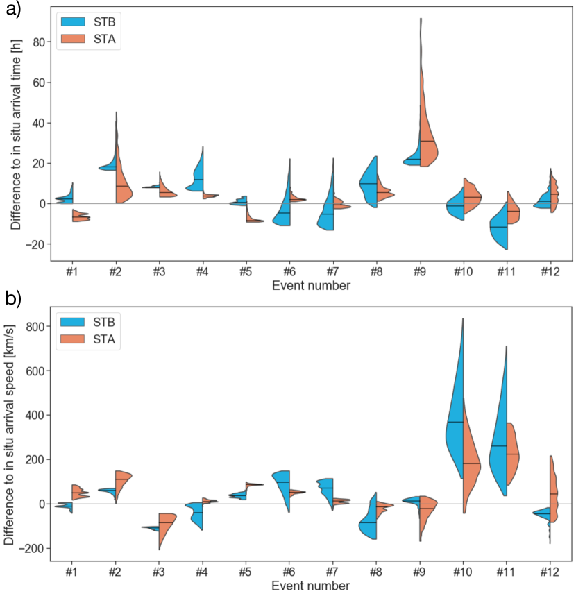
Figure 7 shows the distributions of the arrival time and arrival speed differences with respect to the in situ arrivals for all ensemble members for each CME. Blue and orange correspond to STB and STA ensemble predictions, respectively. The black horizontal lines indicate the median values of each distribution. When comparing the median predicted arrival times to the in situ arrivals, we obtain a mean absolute error (MAE) over all events of hrs and a root mean square error (RMSE) of hrs. A mean error (ME) of hrs indicates, in this setup, that ELEvoHI tends to predict the arrivals too late. The highest arrival time discrepancy is found for event 9 where the prediction based on STA is 31 hrs too late. When comparing the median predicted arrival speeds to the in situ speeds we get a MAE of 87 111 km s-1, a RMSE of 123 km s-1 and a ME of 52 km s-1. The highest speed difference is found for the STB prediction of event 10, overestimating the arrival speed by 369 km s-1.
Interestingly, event 10 gives an accurate predicted arrival time, even though the predicted arrival speed is highly overestimated. When performing GCS reconstruction we obtain a high latitude and a large tilt angle for this CME meaning that the 3D propagation direction differs from that in the ecliptic plane (see Table 2). As already mentioned, event 11 is a CME-CME interaction event which explains the large discrepancy especially for the predicted arrival speed. The reason might be found in an extremely low drag due to preconditioning in the interplanetary space (Rollett \BOthers., \APACyear2014; Y\BPBID. Liu \BOthers., \APACyear2014; Temmer \BBA Nitta, \APACyear2015).
5 Discussion and Conclusions
We present the ELEvoHI ensemble modeling results for 12 CMEs, occurring between February 2010 and July 2012, that were observed by both STEREO spacecraft. This study mainly focuses on the difference of the modeled arrival time and arrival speed when using STA and STB HI observations, separately. We find on average a difference of 6.5 hrs between arrival time predictions from the two spacecraft but the largest difference is about 9.5 hrs for event . For the arrival speed we find a mean difference between STA and STB predictions of 63 km s-1 with a maximum difference of 189 km s-1 for event .
ELEvoHI tends to predict the arrival time later than observed for CMEs that are considered as ’flank hits’ (event and event ). For such events the propagation direction with respect to Earth is larger than 20°, and not all of the ensemble members predict an Earth impact. The reason for the late arrival prediction may be found in the assumed circular shape (for ) and the highly curved flanks.
We provide two CME arrival time and arrival speed predictions, from STA and STB observation, for the same CME to examine the reasons for the discrepancy between these two predictions. We find, that the CME front propagates in different ambient solar wind conditions when observed in STA and STB HI images. However the kinematics of the CME front obtained e.g. by STA data is used for modeling of the whole CME front, including the Earth-directed part. The same applies for predictions based on STB data, which is the reason for the differences in the predicted arrival times based on STA and STB observations.
We further see, that an ambient solar wind exhibiting a high variance within the area used for ELEvoHI model predictions leads to larger discrepancies between STA and STB model predictions. We obtain a Pearson correlation coefficient (), when excluding flank hits (events and event ) and the CME-CME interaction event (event ). Furthermore, we assume that in such cases the CME front is more likely to deform from an idealized elliptical shape due to interaction with the ambient solar wind (Riley \BBA Crooker, \APACyear2004; Owens \BOthers., \APACyear2017).
The current CME forecasting abilities in the community are summarized in Riley \BOthers. (\APACyear2018). They analyzed CME forecasts that have been submitted to the Community Coordinated Modeling Center (CCMC) scoreboard from 2013 to mid-2018. The CCMC scoreboard is a platform provided to scientists to compare their forecasts with each other in real-time. Riley \BOthers. (\APACyear2018) found that the CME shock arrival times for all models combined are predicted on average within hrs but with standard deviations of sometimes more than 20 hrs. The best model performance was found for the WSA-ENLIL+Cone model (Odstrcil \BOthers., \APACyear2004), run by the UK Met Office, having a bias of 1 hour, a MAE of 13 hrs and a standard deviation of 15 hrs. The results of this study are similar to the findings of Riley \BOthers. (\APACyear2018) when comparing the modeled arrival times to the actual arrivals of CMEs, as determined from in situ measurements. Here, we only perform hindcasts of CME arrivals. For the 24 arrival predictions (12 based on STA and 12 based on STB observations), we obtain a MAE of hrs, a RMSE of hrs and a ME of hrs for the arrival time. For the arrival speed, we get a MAE of 87 111 km s-1, a RMSE of 123 km s-1 and a ME of 52 km s-1.
As already mentioned, event 11 is a CME-CME interaction event studied e.g. by Kubicka \BOthers. (\APACyear2016). This CME was closely preceded by two other CMEs that erupted one and two days before this event and that altered the conditions in the heliosphere. The arrival time prediction for this CME is about 11 hrs too early, while the arrival speed is greatly overestimated (by 260 km s-1) using the ambient solar wind solutions provided by the WSA/HUX model. However, this model does not consider preceding CMEs and is likely not valid in such cases. An additional approach to infer the ambient solar wind conditions in the low heliosphere is shown in Barnard \BOthers. (\APACyear2019). In this study the authors established a statistical relationship between the solar wind speed in the low heliosphere and the variability in HI images. A recent study by Amerstorfer \BOthers. (\APACyear2021) focuses on different input parameters to ELEvoHI including three possible methods to infer the ambient solar wind conditions needed by the model. First, the ambient solar wind speed is obtained from in-situ measurements at 1 AU. Second, the solar wind speed is based on an statistical approach using 14 years of OMNI data. Third, an estimate of the ambient solar wind speed is obtained from the WSA-HUX model combination. In their study, Amerstorfer \BOthers. (\APACyear2021) concluded that the third approach provides the best results.
ELEvoHI provides ensemble predictions based on various inputs, namely propagation direction, half width, inverse aspect ratio and ambient solar wind speed. In the current version, ELEvoHI is not able to react to possible deflections of a CME during its propagation. Furthermore, the elliptical CME shape, once defined by the input parameters, does not change during propagation. This has been shown to be invalid by, for example, Rollett \BOthers. (\APACyear2014), who performed a case study by combining HI data with in situ data to ascertain the kinematics of the 2012, March 7 CME. The authors demonstrated evidence for an asymmetric evolution of the CME, which was caused by the preconditioned ambient solar wind resulting in a different drag regime influencing different parts of the CME.
CME deflection (e.g. Y. Wang \BOthers., \APACyear2004, \APACyear2014) and deformation (e.g. Barnard \BOthers., \APACyear2017; Kay \BBA Nieves-Chinchilla, \APACyear2020) are important factors when considering CME propagation in the heliosphere. The authors found that the failure to take these factors into account would likely lead to uncertainties in the arrival time and arrival speed prediction. Barnard \BOthers. (\APACyear2017) additionally showed that different tracks lead to quite different CME arrival time predictions. By using HI observations with better solar wind modeling and varying CME frontal shapes we should be able to improve our current arrival time predictions (Barnard \BOthers., \APACyear2020).
A number of studies have taken advantage of stereoscopic HI observations, from the two STEREO spacecraft, to glean information on CME propagation and evolution (e.g. Y. Liu \BOthers., \APACyear2010; Lugaz, \APACyear2010; Davies \BOthers., \APACyear2013; Volpes \BBA Bothmer, \APACyear2015). Braga \BOthers. (\APACyear2020) studied 14 CMEs using the drag model and a modified version of the ELCon model, to get the CME parameters (e.g. , , ) based on HI observations from both STEREO spacecraft simultaneously. For the five events, that are also included in our study, we obtain similar results as Braga \BOthers. (\APACyear2020). Please note that we run ELEvoHI in ensemble mode in this study. We believe, that a stereoscopic view on CMEs incorporated in ELEvoHI will improve the arrival time predictions substantially. Therefore, we strongly support ESA’s L5 mission, equipped with a heliospheric imager (Lavraud \BOthers., \APACyear2016; Kraft \BOthers., \APACyear2017), and an additional heliospheric imager at L1. Fortunately, the upcoming Earth-orbiting PUNCH mission (launch planned in 2023) will also possess wide-angle white-light heliospheric imagers, as well as a coronagraph, and will be able to provide additional observations of CMEs. Based on information from these additional vantage points, more accurate CME arrival predictions are likely to be achieved. Since ELEvoHI is ready to be used in near real-time, future HI observations are essential for further CME arrival predictions. STA, currently near L5, will have moved beyond L4 by 2027, so it will be necessary to have heliospheric imagers that are observing the space between Sun and Earth after around 2030.
In a next step, we want to further develop ELEvoHI in such a way that it can combine HI data from two vantage points in order to constrain the CME and exclude ensemble runs that are not consistent with the observations. Also the CME shape can be constrained by multiple HI observations and therefore, we aim to make the CME front deformable during the propagation through the heliosphere. Hence, the assumed elliptical CME front would be able to adjust according to the ambient solar wind conditions. It was already shown in previous studies (e.g. Scott \BOthers., \APACyear2019; Chi \BOthers., \APACyear2020) that ghost fronts in the HI observations can be used to infer the structure of a CME. Using their approach, we also aim to improve our model by verifying and constraining the CME shape.
6 Data Sources
Data
STEREO/HI: https://www.ukssdc.ac.uk/solar/stereo/data.html
STEREO/COR2 and SoHO/LASCO: https://sdac.virtualsolar.org/cgi/
NSO/GONG: https://gong.nso.edu/data/magmap/
HELCATS: https://www.helcats-fp7.eu
ICMECAT: https://doi.org/10.6084/m9.figshare.6356420
Model
ELEvoHI is available at https://zenodo.org/record/3873420.
EAGEL is available at https://zenodo.org/record/4154458.
Results
The visualization of each prediction result, i.e. movies and figures, can be downloaded from https://doi.org/10.6084/m9.figshare.12758312.
Software
IDLTM Version 8.4
Python 3.7.6
SATPLOT: https://hesperia.gsfc.nasa.gov/ssw/stereo/secchi/idl/jpl/satplot/SATPLOT_User_Guide.pdf
Acknowledgements.
T.A., J.H., M.B., M.A.R., C.M., A.J.W., R.L.B, and U.V.A. thank the Austrian Science Fund (FWF): P31265-N27, J4160-N27, P31659-N27, P31521-N27.References
- Altschuler \BBA Newkirk (\APACyear1969) \APACinsertmetastaraltschuler69{APACrefauthors}Altschuler, M\BPBID.\BCBT \BBA Newkirk, G. \APACrefYearMonthDay1969\APACmonth09. \BBOQ\APACrefatitleMagnetic Fields and the Structure of the Solar Corona. I: Methods of Calculating Coronal Fields Magnetic Fields and the Structure of the Solar Corona. I: Methods of Calculating Coronal Fields.\BBCQ \APACjournalVolNumPagesSol. Phys.9131-149. {APACrefDOI} 10.1007/BF00145734 \PrintBackRefs\CurrentBib
- Amerstorfer \BOthers. (\APACyear2021) \APACinsertmetastarAmerstorfer2021{APACrefauthors}Amerstorfer, T., Hinterreiter, J., Reiss, M\BPBIA., Möstl, C., Davies, J\BPBIA., Bailey, R\BPBIL.\BDBLHarrison, R\BPBIA. \APACrefYearMonthDay2021. \BBOQ\APACrefatitleEvaluation of CME Arrival Prediction Using Ensemble Modeling Based on Heliospheric Imaging Observations Evaluation of cme arrival prediction using ensemble modeling based on heliospheric imaging observations.\BBCQ \APACjournalVolNumPagesSpace Weather191e2020SW002553. {APACrefURL} https://agupubs.onlinelibrary.wiley.com/doi/abs/10.1029/2020SW002553 \APACrefnotee2020SW002553 10.1029/2020SW002553 {APACrefDOI} https://doi.org/10.1029/2020SW002553 \PrintBackRefs\CurrentBib
- Amerstorfer \BOthers. (\APACyear2018) \APACinsertmetastarAmerstorfer2018{APACrefauthors}Amerstorfer, T., Möstl, C., Hess, P., Temmer, M., Mays, M\BPBIL., Reiss, M\BPBIA.\BDBLBourdin, P\BPBIA. \APACrefYearMonthDay2018\APACmonth07. \BBOQ\APACrefatitleEnsemble Prediction of a Halo Coronal Mass Ejection Using Heliospheric Imagers Ensemble Prediction of a Halo Coronal Mass Ejection Using Heliospheric Imagers.\BBCQ \APACjournalVolNumPagesSpace Weather167784-801. {APACrefDOI} 10.1029/2017SW001786 \PrintBackRefs\CurrentBib
- Arge \BOthers. (\APACyear2003) \APACinsertmetastararge03{APACrefauthors}Arge, C\BPBIN., Odstrcil, D., Pizzo, V\BPBIJ.\BCBL \BBA Mayer, L\BPBIR. \APACrefYearMonthDay2003\APACmonth09. \BBOQ\APACrefatitleImproved Method for Specifying Solar Wind Speed Near the Sun Improved Method for Specifying Solar Wind Speed Near the Sun.\BBCQ \BIn M. Velli, R. Bruno, F. Malara\BCBL \BBA B. Bucci (\BEDS), \APACrefbtitleSolar Wind Ten Solar wind ten (\BVOL 679, \BPG 190-193). {APACrefDOI} 10.1063/1.1618574 \PrintBackRefs\CurrentBib
- Barnard \BOthers. (\APACyear2020) \APACinsertmetastarBarnard2020{APACrefauthors}Barnard, L., Owens, M\BPBIJ., Scott, C\BPBIJ.\BCBL \BBA de Koning, C\BPBIA. \APACrefYearMonthDay2020. \BBOQ\APACrefatitleEnsemble CME Modeling Constrained by Heliospheric Imager Observations Ensemble cme modeling constrained by heliospheric imager observations.\BBCQ \APACjournalVolNumPagesAGU Advances13e2020AV000214. {APACrefURL} https://agupubs.onlinelibrary.wiley.com/doi/abs/10.1029/2020AV000214 \APACrefnotee2020AV000214 10.1029/2020AV000214 {APACrefDOI} 10.1029/2020AV000214 \PrintBackRefs\CurrentBib
- Barnard \BOthers. (\APACyear2017) \APACinsertmetastarBarnard2017{APACrefauthors}Barnard, L\BPBIA., de Koning, C\BPBIA., Scott, C\BPBIJ., Owens, M\BPBIJ., Wilkinson, J.\BCBL \BBA Davies, J\BPBIA. \APACrefYearMonthDay2017\APACmonth06. \BBOQ\APACrefatitleTesting the current paradigm for space weather prediction with heliospheric imagers Testing the current paradigm for space weather prediction with heliospheric imagers.\BBCQ \APACjournalVolNumPagesSpace Weather156782-803. {APACrefDOI} 10.1002/2017SW001609 \PrintBackRefs\CurrentBib
- Barnard \BOthers. (\APACyear2019) \APACinsertmetastarBarnard2019{APACrefauthors}Barnard, L\BPBIA., Owens, M\BPBIJ., Scott, C\BPBIJ.\BCBL \BBA Jones, S\BPBIR. \APACrefYearMonthDay2019\APACmonth06. \BBOQ\APACrefatitleExtracting Inner-Heliosphere Solar Wind Speed Information From Heliospheric Imager Observations Extracting Inner-Heliosphere Solar Wind Speed Information From Heliospheric Imager Observations.\BBCQ \APACjournalVolNumPagesSpace Weather176925-938. {APACrefDOI} 10.1029/2019SW002226 \PrintBackRefs\CurrentBib
- Braga \BOthers. (\APACyear2020) \APACinsertmetastarBraga2020{APACrefauthors}Braga, C\BPBIR., Vourlidas, A., Stenborg, G., Dal Lago, A., Mendonça, R\BPBIR\BPBIS\BPBId.\BCBL \BBA Echer, E. \APACrefYearMonthDay2020\APACmonth09. \BBOQ\APACrefatitlePredicting the Time of Arrival of Coronal Mass Ejections at Earth From Heliospheric Imaging Observations Predicting the Time of Arrival of Coronal Mass Ejections at Earth From Heliospheric Imaging Observations.\BBCQ \APACjournalVolNumPagesJournal of Geophysical Research (Space Physics)1259e27885. {APACrefDOI} 10.1029/2020JA027885 \PrintBackRefs\CurrentBib
- Brueckner \BOthers. (\APACyear1995) \APACinsertmetastarBrueckner1995{APACrefauthors}Brueckner, G\BPBIE., Howard, R\BPBIA., Koomen, M\BPBIJ., Korendyke, C\BPBIM., Michels, D\BPBIJ., Moses, J\BPBID.\BDBLEyles, C\BPBIJ. \APACrefYearMonthDay1995\APACmonth12. \BBOQ\APACrefatitleThe Large Angle Spectroscopic Coronagraph (LASCO) The Large Angle Spectroscopic Coronagraph (LASCO).\BBCQ \APACjournalVolNumPagesSol. Phys.1621-2357-402. {APACrefDOI} 10.1007/BF00733434 \PrintBackRefs\CurrentBib
- Cannon (\APACyear2013) \APACinsertmetastarCannon2013{APACrefauthors}Cannon, P\BPBIS. \APACrefYearMonthDay2013\APACmonth04. \BBOQ\APACrefatitleExtreme Space Weather—A Report Published by the UK Royal Academy of Engineering Extreme Space Weather—A Report Published by the UK Royal Academy of Engineering.\BBCQ \APACjournalVolNumPagesSpace Weather114138-139. {APACrefDOI} 10.1002/swe.20032 \PrintBackRefs\CurrentBib
- Chi \BOthers. (\APACyear2020) \APACinsertmetastarChi2020{APACrefauthors}Chi, Y., Scott, C., Shen, C., Owens, M., Lang, M., Xu, M.\BDBLLockwood, M. \APACrefYearMonthDay2020\APACmonth08. \BBOQ\APACrefatitleUsing the “Ghost Front” to Predict the Arrival Time and Speed of CMEs at Venus and Earth Using the “Ghost Front” to Predict the Arrival Time and Speed of CMEs at Venus and Earth.\BBCQ \APACjournalVolNumPagesApJ8992143. {APACrefDOI} 10.3847/1538-4357/aba95a \PrintBackRefs\CurrentBib
- Davies \BOthers. (\APACyear2012) \APACinsertmetastarDavies2012{APACrefauthors}Davies, J\BPBIA., Harrison, R\BPBIA., Perry, C\BPBIH., Möstl, C., Lugaz, N., Rollett, T.\BDBLSavani, N\BPBIP. \APACrefYearMonthDay2012\APACmonth05. \BBOQ\APACrefatitleA Self-similar Expansion Model for Use in Solar Wind Transient Propagation Studies A Self-similar Expansion Model for Use in Solar Wind Transient Propagation Studies.\BBCQ \APACjournalVolNumPagesApJ750123. {APACrefDOI} 10.1088/0004-637X/750/1/23 \PrintBackRefs\CurrentBib
- Davies \BOthers. (\APACyear2009) \APACinsertmetastarDavies2009{APACrefauthors}Davies, J\BPBIA., Harrison, R\BPBIA., Rouillard, A\BPBIP., Sheeley, N\BPBIR., Perry, C\BPBIH., Bewsher, D.\BDBLBrown, D\BPBIS. \APACrefYearMonthDay2009\APACmonth01. \BBOQ\APACrefatitleA synoptic view of solar transient evolution in the inner heliosphere using the Heliospheric Imagers on STEREO A synoptic view of solar transient evolution in the inner heliosphere using the Heliospheric Imagers on STEREO.\BBCQ \APACjournalVolNumPagesGeophys. Res. Lett.362L02102. {APACrefDOI} 10.1029/2008GL036182 \PrintBackRefs\CurrentBib
- Davies \BOthers. (\APACyear2013) \APACinsertmetastarDavies2013{APACrefauthors}Davies, J\BPBIA., Perry, C\BPBIH., Trines, R\BPBIM\BPBIG\BPBIM., Harrison, R\BPBIA., Lugaz, N., Möstl, C.\BDBLSteed, K. \APACrefYearMonthDay2013\APACmonth11. \BBOQ\APACrefatitleEstablishing a Stereoscopic Technique for Determining the Kinematic Properties of Solar Wind Transients based on a Generalized Self-similarly Expanding Circular Geometry Establishing a Stereoscopic Technique for Determining the Kinematic Properties of Solar Wind Transients based on a Generalized Self-similarly Expanding Circular Geometry.\BBCQ \APACjournalVolNumPagesApJ7772167. {APACrefDOI} 10.1088/0004-637X/777/2/167 \PrintBackRefs\CurrentBib
- Dumbović \BOthers. (\APACyear2018) \APACinsertmetastarDumbovic2018{APACrefauthors}Dumbović, M., Čalogović, J., Vršnak, B., Temmer, M., Mays, M\BPBIL., Veronig, A.\BCBL \BBA Piantschitsch, I. \APACrefYearMonthDay2018\APACmonth02. \BBOQ\APACrefatitleThe Drag-based Ensemble Model (DBEM) for Coronal Mass Ejection Propagation The Drag-based Ensemble Model (DBEM) for Coronal Mass Ejection Propagation.\BBCQ \APACjournalVolNumPagesApJ8542180. {APACrefDOI} 10.3847/1538-4357/aaaa66 \PrintBackRefs\CurrentBib
- Eyles \BOthers. (\APACyear2009) \APACinsertmetastarEyles2009{APACrefauthors}Eyles, C\BPBIJ., Harrison, R\BPBIA., Davis, C\BPBIJ., Waltham, N\BPBIR., Shaughnessy, B\BPBIM., Mapson-Menard, H\BPBIC\BPBIA.\BDBLRochus, P. \APACrefYearMonthDay2009\APACmonth02. \BBOQ\APACrefatitleThe Heliospheric Imagers Onboard the STEREO Mission The Heliospheric Imagers Onboard the STEREO Mission.\BBCQ \APACjournalVolNumPagesSol. Phys.2542387-445. {APACrefDOI} 10.1007/s11207-008-9299-0 \PrintBackRefs\CurrentBib
- Gopalswamy \BOthers. (\APACyear2000) \APACinsertmetastarGopalswamy2000{APACrefauthors}Gopalswamy, N., Lara, A., Lepping, R\BPBIP., Kaiser, M\BPBIL., Berdichevsky, D.\BCBL \BBA St. Cyr, O\BPBIC. \APACrefYearMonthDay2000\APACmonth01. \BBOQ\APACrefatitleInterplanetary acceleration of coronal mass ejections Interplanetary acceleration of coronal mass ejections.\BBCQ \APACjournalVolNumPagesGeophys. Res. Lett.272145-148. {APACrefDOI} 10.1029/1999GL003639 \PrintBackRefs\CurrentBib
- Gosling \BOthers. (\APACyear1990) \APACinsertmetastarGosling1990{APACrefauthors}Gosling, J\BPBIT., Bame, S\BPBIJ., McComas, D\BPBIJ.\BCBL \BBA Phillips, J\BPBIL. \APACrefYearMonthDay1990\APACmonth06. \BBOQ\APACrefatitleCoronal mass ejections and large geomagnetic storms Coronal mass ejections and large geomagnetic storms.\BBCQ \APACjournalVolNumPagesGeophys. Res. Lett.177901-904. {APACrefDOI} 10.1029/GL017i007p00901 \PrintBackRefs\CurrentBib
- Harrison \BOthers. (\APACyear2018) \APACinsertmetastarHarrison2018{APACrefauthors}Harrison, R\BPBIA., Davies, J\BPBIA., Barnes, D., Byrne, J\BPBIP., Perry, C\BPBIH., Bothmer, V.\BDBLOdstrčil, D. \APACrefYearMonthDay2018\APACmonth04. \BBOQ\APACrefatitleCMEs in the Heliosphere: I. A Statistical Analysis of the Observational Properties of CMEs Detected in the Heliosphere from 2007 to 2017 by STEREO/HI-1 CMEs in the Heliosphere: I. A Statistical Analysis of the Observational Properties of CMEs Detected in the Heliosphere from 2007 to 2017 by STEREO/HI-1.\BBCQ \APACjournalVolNumPagesSol. Phys.293577. {APACrefDOI} 10.1007/s11207-018-1297-2 \PrintBackRefs\CurrentBib
- Howard \BOthers. (\APACyear2008) \APACinsertmetastarHoward2008{APACrefauthors}Howard, R\BPBIA., Moses, J\BPBID., Vourlidas, A., Newmark, J\BPBIS., Socker, D\BPBIG., Plunkett, S\BPBIP.\BDBLCarter, T. \APACrefYearMonthDay2008\APACmonth04. \BBOQ\APACrefatitleSun Earth Connection Coronal and Heliospheric Investigation (SECCHI) Sun Earth Connection Coronal and Heliospheric Investigation (SECCHI).\BBCQ \APACjournalVolNumPagesSpace Sci. Rev.1361-467-115. {APACrefDOI} 10.1007/s11214-008-9341-4 \PrintBackRefs\CurrentBib
- Hundhausen \BOthers. (\APACyear1994) \APACinsertmetastarHundhausen1994{APACrefauthors}Hundhausen, A\BPBIJ., Stanger, A\BPBIL.\BCBL \BBA Serbicki, S\BPBIA. \APACrefYearMonthDay1994\APACmonth12. \BBOQ\APACrefatitleMass and energy contents of coronal mass ejections: SMM results from 1980 and 1984-1988 Mass and energy contents of coronal mass ejections: SMM results from 1980 and 1984-1988.\BBCQ \BIn J\BPBIJ. Hunt (\BED), \APACrefbtitleSolar Dynamic Phenomena and Solar Wind Consequences, the Third SOHO Workshop Solar dynamic phenomena and solar wind consequences, the third soho workshop (\BVOL 373, \BPG 409). \PrintBackRefs\CurrentBib
- Kaiser \BOthers. (\APACyear2008) \APACinsertmetastarKaiser2008{APACrefauthors}Kaiser, M\BPBIL., Kucera, T\BPBIA., Davila, J\BPBIM., St. Cyr, O\BPBIC., Guhathakurta, M.\BCBL \BBA Christian, E. \APACrefYearMonthDay2008\APACmonth04. \BBOQ\APACrefatitleThe STEREO Mission: An Introduction The STEREO Mission: An Introduction.\BBCQ \APACjournalVolNumPagesSpace Sci. Rev.1361-45-16. {APACrefDOI} 10.1007/s11214-007-9277-0 \PrintBackRefs\CurrentBib
- Kay \BOthers. (\APACyear2020) \APACinsertmetastarKay2020{APACrefauthors}Kay, C., Mays, M\BPBIL.\BCBL \BBA Verbeke, C. \APACrefYearMonthDay2020\APACmonth01. \BBOQ\APACrefatitleIdentifying Critical Input Parameters for Improving Drag-Based CME Arrival Time Predictions Identifying Critical Input Parameters for Improving Drag-Based CME Arrival Time Predictions.\BBCQ \APACjournalVolNumPagesSpace Weather181e02382. {APACrefDOI} 10.1029/2019SW002382 \PrintBackRefs\CurrentBib
- Kay \BBA Nieves-Chinchilla (\APACyear2020) \APACinsertmetastarKayNievesChinchilla2020{APACrefauthors}Kay, C.\BCBT \BBA Nieves-Chinchilla, T. \APACrefYearMonthDay2020\APACmonth11. \BBOQ\APACrefatitleModeling Interplanetary Expansion and Deformation of CMEs with ANTEATR-PARADE I: Relative Contribution of Different Forces Modeling Interplanetary Expansion and Deformation of CMEs with ANTEATR-PARADE I: Relative Contribution of Different Forces.\BBCQ \APACjournalVolNumPagesarXiv e-printsarXiv:2011.06030. \PrintBackRefs\CurrentBib
- Kay \BBA Opher (\APACyear2015) \APACinsertmetastarKayOpher2015{APACrefauthors}Kay, C.\BCBT \BBA Opher, M. \APACrefYearMonthDay2015\APACmonth10. \BBOQ\APACrefatitleThe Heliocentric Distance where the Deflections and Rotations of Solar Coronal Mass Ejections Occur The Heliocentric Distance where the Deflections and Rotations of Solar Coronal Mass Ejections Occur.\BBCQ \APACjournalVolNumPagesApJ8112L36. {APACrefDOI} 10.1088/2041-8205/811/2/L36 \PrintBackRefs\CurrentBib
- Kilpua \BOthers. (\APACyear2012) \APACinsertmetastarKilpua2012{APACrefauthors}Kilpua, E\BPBIK\BPBIJ., Jian, L\BPBIK., Li, Y., Luhmann, J\BPBIG.\BCBL \BBA Russell, C\BPBIT. \APACrefYearMonthDay2012\APACmonth11. \BBOQ\APACrefatitleObservations of ICMEs and ICME-like Solar Wind Structures from 2007 - 2010 Using Near-Earth and STEREO Observations Observations of ICMEs and ICME-like Solar Wind Structures from 2007 - 2010 Using Near-Earth and STEREO Observations.\BBCQ \APACjournalVolNumPagesSol. Phys.2811391-409. {APACrefDOI} 10.1007/s11207-012-9957-0 \PrintBackRefs\CurrentBib
- Kraft \BOthers. (\APACyear2017) \APACinsertmetastarKraft2017{APACrefauthors}Kraft, S., Puschmann, K\BPBIG.\BCBL \BBA Luntama, J\BPBIP. \APACrefYearMonthDay2017. \BBOQ\APACrefatitleRemote sensing optical instrumentation for enhanced space weather monitoring from the L1 and L5 Lagrange points Remote sensing optical instrumentation for enhanced space weather monitoring from the L1 and L5 Lagrange points.\BBCQ \BIn B. Cugny, N. Karafolas\BCBL \BBA Z. Sodnik (\BEDS), \APACrefbtitleInternational Conference on Space Optics — ICSO 2016 International conference on space optics — icso 2016 (\BVOL 10562, \BPGS 115 – 123). \APACaddressPublisherSPIE. {APACrefURL} https://doi.org/10.1117/12.2296100 {APACrefDOI} 10.1117/12.2296100 \PrintBackRefs\CurrentBib
- Kubicka \BOthers. (\APACyear2016) \APACinsertmetastarKubicka2016{APACrefauthors}Kubicka, M., Möstl, C., Amerstorfer, T., Boakes, P\BPBID., Feng, L., Eastwood, J\BPBIP.\BCBL \BBA Törmänen, O. \APACrefYearMonthDay2016\APACmonth12. \BBOQ\APACrefatitlePrediction of Geomagnetic Storm Strength from Inner Heliospheric In Situ Observations Prediction of Geomagnetic Storm Strength from Inner Heliospheric In Situ Observations.\BBCQ \APACjournalVolNumPagesApJ8332255. {APACrefDOI} 10.3847/1538-4357/833/2/255 \PrintBackRefs\CurrentBib
- Lavraud \BOthers. (\APACyear2016) \APACinsertmetastarLavraud2016{APACrefauthors}Lavraud, B., Liu, Y., Segura, K., He, J., Qin, G., Temmer, M.\BDBLFernández, J\BPBIG. \APACrefYearMonthDay2016\APACmonth08. \BBOQ\APACrefatitleA small mission concept to the Sun-Earth Lagrangian L5 point for innovative solar, heliospheric and space weather science A small mission concept to the Sun-Earth Lagrangian L5 point for innovative solar, heliospheric and space weather science.\BBCQ \APACjournalVolNumPagesJournal of Atmospheric and Solar-Terrestrial Physics146171-185. {APACrefDOI} 10.1016/j.jastp.2016.06.004 \PrintBackRefs\CurrentBib
- Y. Liu \BOthers. (\APACyear2010) \APACinsertmetastarLiu2010A{APACrefauthors}Liu, Y., Davies, J\BPBIA., Luhmann, J\BPBIG., Vourlidas, A., Bale, S\BPBID.\BCBL \BBA Lin, R\BPBIP. \APACrefYearMonthDay2010\APACmonth02. \BBOQ\APACrefatitleGeometric Triangulation of Imaging Observations to Track Coronal Mass Ejections Continuously Out to 1 AU Geometric Triangulation of Imaging Observations to Track Coronal Mass Ejections Continuously Out to 1 AU.\BBCQ \APACjournalVolNumPagesApJ7101L82-L87. {APACrefDOI} 10.1088/2041-8205/710/1/L82 \PrintBackRefs\CurrentBib
- Y\BPBID. Liu \BOthers. (\APACyear2014) \APACinsertmetastarLiu2014{APACrefauthors}Liu, Y\BPBID., Luhmann, J\BPBIG., Kajdič, P., Kilpua, E\BPBIK\BPBIJ., Lugaz, N., Nitta, N\BPBIV.\BDBLGalvin, A\BPBIB. \APACrefYearMonthDay2014\APACmonth03. \BBOQ\APACrefatitleObservations of an extreme storm in interplanetary space caused by successive coronal mass ejections Observations of an extreme storm in interplanetary space caused by successive coronal mass ejections.\BBCQ \APACjournalVolNumPagesNature Communications53481. {APACrefDOI} 10.1038/ncomms4481 \PrintBackRefs\CurrentBib
- Lugaz (\APACyear2010) \APACinsertmetastarLugaz2010{APACrefauthors}Lugaz, N. \APACrefYearMonthDay2010\APACmonth12. \BBOQ\APACrefatitleAccuracy and Limitations of Fitting and Stereoscopic Methods to Determine the Direction of Coronal Mass Ejections from Heliospheric Imagers Observations Accuracy and Limitations of Fitting and Stereoscopic Methods to Determine the Direction of Coronal Mass Ejections from Heliospheric Imagers Observations.\BBCQ \APACjournalVolNumPagesSol. Phys.2672411-429. {APACrefDOI} 10.1007/s11207-010-9654-9 \PrintBackRefs\CurrentBib
- Lugaz \BOthers. (\APACyear2012) \APACinsertmetastarLugaz2012{APACrefauthors}Lugaz, N., Farrugia, C\BPBIJ., Davies, J\BPBIA., Möstl, C., Davis, C\BPBIJ., Roussev, I\BPBII.\BCBL \BBA Temmer, M. \APACrefYearMonthDay2012\APACmonth11. \BBOQ\APACrefatitleThe Deflection of the Two Interacting Coronal Mass Ejections of 2010 May 23-24 as Revealed by Combined in Situ Measurements and Heliospheric Imaging The Deflection of the Two Interacting Coronal Mass Ejections of 2010 May 23-24 as Revealed by Combined in Situ Measurements and Heliospheric Imaging.\BBCQ \APACjournalVolNumPagesApJ759168. {APACrefDOI} 10.1088/0004-637X/759/1/68 \PrintBackRefs\CurrentBib
- Lugaz \BOthers. (\APACyear2010) \APACinsertmetastarLugazEtAl2010{APACrefauthors}Lugaz, N., Hernandez-Charpak, J\BPBIN., Roussev, I\BPBII., Davis, C\BPBIJ., Vourlidas, A.\BCBL \BBA Davies, J\BPBIA. \APACrefYearMonthDay2010\APACmonth05. \BBOQ\APACrefatitleDetermining the Azimuthal Properties of Coronal Mass Ejections from Multi-Spacecraft Remote-Sensing Observations with STEREO SECCHI Determining the Azimuthal Properties of Coronal Mass Ejections from Multi-Spacecraft Remote-Sensing Observations with STEREO SECCHI.\BBCQ \APACjournalVolNumPagesApJ7151493-499. {APACrefDOI} 10.1088/0004-637X/715/1/493 \PrintBackRefs\CurrentBib
- Luhmann \BOthers. (\APACyear2008) \APACinsertmetastarLuhmann2008{APACrefauthors}Luhmann, J\BPBIG., Curtis, D\BPBIW., Schroeder, P., McCauley, J., Lin, R\BPBIP., Larson, D\BPBIE.\BDBLGosling, J\BPBIT. \APACrefYearMonthDay2008\APACmonth04. \BBOQ\APACrefatitleSTEREO IMPACT Investigation Goals, Measurements, and Data Products Overview STEREO IMPACT Investigation Goals, Measurements, and Data Products Overview.\BBCQ \APACjournalVolNumPagesSpace Sci. Rev.1361-4117-184. {APACrefDOI} 10.1007/s11214-007-9170-x \PrintBackRefs\CurrentBib
- Manoharan \BOthers. (\APACyear2004) \APACinsertmetastarManoharan2004{APACrefauthors}Manoharan, P\BPBIK., Gopalswamy, N., Yashiro, S., Lara, A., Michalek, G.\BCBL \BBA Howard, R\BPBIA. \APACrefYearMonthDay2004\APACmonth06. \BBOQ\APACrefatitleInfluence of coronal mass ejection interaction on propagation of interplanetary shocks Influence of coronal mass ejection interaction on propagation of interplanetary shocks.\BBCQ \APACjournalVolNumPagesJournal of Geophysical Research (Space Physics)109A6A06109. {APACrefDOI} 10.1029/2003JA010300 \PrintBackRefs\CurrentBib
- Manoharan \BBA Mujiber Rahman (\APACyear2011) \APACinsertmetastarManoharan2011{APACrefauthors}Manoharan, P\BPBIK.\BCBT \BBA Mujiber Rahman, A. \APACrefYearMonthDay2011\APACmonth04. \BBOQ\APACrefatitleCoronal mass ejections—Propagation time and associated internal energy Coronal mass ejections—Propagation time and associated internal energy.\BBCQ \APACjournalVolNumPagesJournal of Atmospheric and Solar-Terrestrial Physics735-6671-677. {APACrefDOI} 10.1016/j.jastp.2011.01.017 \PrintBackRefs\CurrentBib
- Mierla \BOthers. (\APACyear2010) \APACinsertmetastarMierla2010{APACrefauthors}Mierla, M., Inhester, B., Antunes, A., Boursier, Y., Byrne, J\BPBIP., Colaninno, R.\BDBLZhukov, A\BPBIN. \APACrefYearMonthDay2010\APACmonth01. \BBOQ\APACrefatitleOn the 3-D reconstruction of Coronal Mass Ejections using coronagraph data On the 3-D reconstruction of Coronal Mass Ejections using coronagraph data.\BBCQ \APACjournalVolNumPagesAnnales Geophysicae281203-215. {APACrefDOI} 10.5194/angeo-28-203-2010 \PrintBackRefs\CurrentBib
- Möstl \BBA Davies (\APACyear2013) \APACinsertmetastarMoestlDavies2013{APACrefauthors}Möstl, C.\BCBT \BBA Davies, J\BPBIA. \APACrefYearMonthDay2013\APACmonth07. \BBOQ\APACrefatitleSpeeds and Arrival Times of Solar Transients Approximated by Self-similar Expanding Circular Fronts Speeds and Arrival Times of Solar Transients Approximated by Self-similar Expanding Circular Fronts.\BBCQ \APACjournalVolNumPagesSol. Phys.2851-2411-423. {APACrefDOI} 10.1007/s11207-012-9978-8 \PrintBackRefs\CurrentBib
- Möstl \BOthers. (\APACyear2017) \APACinsertmetastarMoestl2017{APACrefauthors}Möstl, C., Isavnin, A., Boakes, P\BPBID., Kilpua, E\BPBIK\BPBIJ., Davies, J\BPBIA., Harrison, R\BPBIA.\BDBLZhang, T\BPBIL. \APACrefYearMonthDay2017\APACmonth07. \BBOQ\APACrefatitleModeling observations of solar coronal mass ejections with heliospheric imagers verified with the Heliophysics System Observatory Modeling observations of solar coronal mass ejections with heliospheric imagers verified with the Heliophysics System Observatory.\BBCQ \APACjournalVolNumPagesSpace Weather157955-970. {APACrefDOI} 10.1002/2017SW001614 \PrintBackRefs\CurrentBib
- Möstl \BOthers. (\APACyear2015) \APACinsertmetastarMoestl2015{APACrefauthors}Möstl, C., Rollett, T., Frahm, R\BPBIA., Liu, Y\BPBID., Long, D\BPBIM., Colaninno, R\BPBIC.\BDBLVršnak, B. \APACrefYearMonthDay2015\APACmonth05. \BBOQ\APACrefatitleStrong coronal channelling and interplanetary evolution of a solar storm up to Earth and Mars Strong coronal channelling and interplanetary evolution of a solar storm up to Earth and Mars.\BBCQ \APACjournalVolNumPagesNature Communications67135. {APACrefDOI} 10.1038/ncomms8135 \PrintBackRefs\CurrentBib
- Möstl \BOthers. (\APACyear2011) \APACinsertmetastarMoestl2011{APACrefauthors}Möstl, C., Rollett, T., Lugaz, N., Farrugia, C\BPBIJ., Davies, J\BPBIA., Temmer, M.\BDBLBiernat, H\BPBIK. \APACrefYearMonthDay2011\APACmonth11. \BBOQ\APACrefatitleArrival Time Calculation for Interplanetary Coronal Mass Ejections with Circular Fronts and Application to STEREO Observations of the 2009 February 13 Eruption Arrival Time Calculation for Interplanetary Coronal Mass Ejections with Circular Fronts and Application to STEREO Observations of the 2009 February 13 Eruption.\BBCQ \APACjournalVolNumPagesApJ741134. {APACrefDOI} 10.1088/0004-637X/741/1/34 \PrintBackRefs\CurrentBib
- Möstl \BOthers. (\APACyear2020) \APACinsertmetastarMoestl2020{APACrefauthors}Möstl, C., Weiss, A\BPBIJ., Bailey, R\BPBIL., Reiss, M\BPBIA., Amerstorfer, U\BPBIV., Amerstorfer, T.\BDBLStansby, D. \APACrefYearMonthDay2020\APACmonth07. \BBOQ\APACrefatitlePrediction of the in situ coronal mass ejection rate for solar cycle 25: Implications for Parker Solar Probe in situ observations Prediction of the in situ coronal mass ejection rate for solar cycle 25: Implications for Parker Solar Probe in situ observations.\BBCQ \APACjournalVolNumPagesarXiv e-printsarXiv:2007.14743. \PrintBackRefs\CurrentBib
- Nieves-Chinchilla \BOthers. (\APACyear2018) \APACinsertmetastarNieves_Chinchilla2018{APACrefauthors}Nieves-Chinchilla, T., Vourlidas, A., Raymond, J\BPBIC., Linton, M\BPBIG., Al-haddad, N., Savani, N\BPBIP.\BDBLHidalgo, M\BPBIA. \APACrefYearMonthDay2018\APACmonth02. \BBOQ\APACrefatitleUnderstanding the Internal Magnetic Field Configurations of ICMEs Using More than 20 Years of Wind Observations Understanding the Internal Magnetic Field Configurations of ICMEs Using More than 20 Years of Wind Observations.\BBCQ \APACjournalVolNumPagesSol. Phys.293225. {APACrefDOI} 10.1007/s11207-018-1247-z \PrintBackRefs\CurrentBib
- Odstrcil \BOthers. (\APACyear2004) \APACinsertmetastarOdstrcil2004{APACrefauthors}Odstrcil, D., Pizzo, V\BPBIJ., Linker, J\BPBIA., Riley, P., Lionello, R.\BCBL \BBA Mikic, Z. \APACrefYearMonthDay2004\APACmonth10. \BBOQ\APACrefatitleInitial coupling of coronal and heliospheric numerical magnetohydrodynamic codes Initial coupling of coronal and heliospheric numerical magnetohydrodynamic codes.\BBCQ \APACjournalVolNumPagesJournal of Atmospheric and Solar-Terrestrial Physics6615-161311-1320. {APACrefDOI} 10.1016/j.jastp.2004.04.007 \PrintBackRefs\CurrentBib
- Owens \BOthers. (\APACyear2017) \APACinsertmetastarOwens2017Nat{APACrefauthors}Owens, M\BPBIJ., Lockwood, M.\BCBL \BBA Barnard, L\BPBIA. \APACrefYearMonthDay2017\APACmonth06. \BBOQ\APACrefatitleCoronal mass ejections are not coherent magnetohydrodynamic structures Coronal mass ejections are not coherent magnetohydrodynamic structures.\BBCQ \APACjournalVolNumPagesScientific Reports74152. {APACrefDOI} 10.1038/s41598-017-04546-3 \PrintBackRefs\CurrentBib
- Owens \BOthers. (\APACyear2020) \APACinsertmetastarOwens2020{APACrefauthors}Owens, M\BPBIJ., Lockwood, M.\BCBL \BBA Barnard, L\BPBIA. \APACrefYearMonthDay2020. \BBOQ\APACrefatitleThe Value of CME Arrival Time Forecasts for Space Weather Mitigation The value of cme arrival time forecasts for space weather mitigation.\BBCQ \APACjournalVolNumPagesSpace Weather189e2020SW002507. {APACrefURL} https://agupubs.onlinelibrary.wiley.com/doi/abs/10.1029/2020SW002507 \APACrefnotee2020SW002507 10.1029/2020SW002507 {APACrefDOI} 10.1029/2020SW002507 \PrintBackRefs\CurrentBib
- Owens \BBA Riley (\APACyear2017) \APACinsertmetastarOwens2017{APACrefauthors}Owens, M\BPBIJ.\BCBT \BBA Riley, P. \APACrefYearMonthDay2017\APACmonth11. \BBOQ\APACrefatitleProbabilistic Solar Wind Forecasting Using Large Ensembles of Near-Sun Conditions With a Simple One-Dimensional “Upwind” Scheme Probabilistic Solar Wind Forecasting Using Large Ensembles of Near-Sun Conditions With a Simple One-Dimensional “Upwind” Scheme.\BBCQ \APACjournalVolNumPagesSpace Weather15111461-1474. {APACrefDOI} 10.1002/2017SW001679 \PrintBackRefs\CurrentBib
- Paouris \BBA Mavromichalaki (\APACyear2017) \APACinsertmetastarPaouris2017{APACrefauthors}Paouris, E.\BCBT \BBA Mavromichalaki, H. \APACrefYearMonthDay2017\APACmonth12. \BBOQ\APACrefatitleEffective Acceleration Model for the Arrival Time of Interplanetary Shocks driven by Coronal Mass Ejections Effective Acceleration Model for the Arrival Time of Interplanetary Shocks driven by Coronal Mass Ejections.\BBCQ \APACjournalVolNumPagesSol. Phys.29212180. {APACrefDOI} 10.1007/s11207-017-1212-2 \PrintBackRefs\CurrentBib
- Pomoell \BBA Poedts (\APACyear2018) \APACinsertmetastarPomoell2018{APACrefauthors}Pomoell, J.\BCBT \BBA Poedts, S. \APACrefYearMonthDay2018\APACmonth06. \BBOQ\APACrefatitleEUHFORIA: European heliospheric forecasting information asset EUHFORIA: European heliospheric forecasting information asset.\BBCQ \APACjournalVolNumPagesJournal of Space Weather and Space Climate8A35. {APACrefDOI} 10.1051/swsc/2018020 \PrintBackRefs\CurrentBib
- Reiss \BOthers. (\APACyear2019) \APACinsertmetastarreiss19{APACrefauthors}Reiss, M\BPBIA., MacNeice, P\BPBIJ., Mays, L\BPBIM., Arge, C\BPBIN., Möstl, C., Nikolic, L.\BCBL \BBA Amerstorfer, T. \APACrefYearMonthDay2019\APACmonth02. \BBOQ\APACrefatitleForecasting the Ambient Solar Wind with Numerical Models. I. On the Implementation of an Operational Framework Forecasting the Ambient Solar Wind with Numerical Models. I. On the Implementation of an Operational Framework.\BBCQ \APACjournalVolNumPagesApJS24035. {APACrefDOI} 10.3847/1538-4365/aaf8b3 \PrintBackRefs\CurrentBib
- Reiss \BOthers. (\APACyear2020) \APACinsertmetastarReiss2020ApJ{APACrefauthors}Reiss, M\BPBIA., MacNeice, P\BPBIJ., Muglach, K., Arge, C\BPBIN., Möstl, C., Riley, P.\BDBLAmerstorfer, U. \APACrefYearMonthDay2020\APACmonth03. \BBOQ\APACrefatitleForecasting the Ambient Solar Wind with Numerical Models. II. An Adaptive Prediction System for Specifying Solar Wind Speed near the Sun Forecasting the Ambient Solar Wind with Numerical Models. II. An Adaptive Prediction System for Specifying Solar Wind Speed near the Sun.\BBCQ \APACjournalVolNumPagesApJ8912165. {APACrefDOI} 10.3847/1538-4357/ab78a0 \PrintBackRefs\CurrentBib
- Richardson \BBA Cane (\APACyear2010) \APACinsertmetastarRichardsonCane2010{APACrefauthors}Richardson, I\BPBIG.\BCBT \BBA Cane, H\BPBIV. \APACrefYearMonthDay2010Jun. \BBOQ\APACrefatitleNear-Earth Interplanetary Coronal Mass Ejections During Solar Cycle 23 (1996 - 2009): Catalog and Summary of Properties Near-Earth Interplanetary Coronal Mass Ejections During Solar Cycle 23 (1996 - 2009): Catalog and Summary of Properties.\BBCQ \APACjournalVolNumPagesSol. Phys.2641189-237. {APACrefDOI} 10.1007/s11207-010-9568-6 \PrintBackRefs\CurrentBib
- Richardson \BBA Cane (\APACyear2012) \APACinsertmetastarRichardsonCane2012{APACrefauthors}Richardson, I\BPBIG.\BCBT \BBA Cane, H\BPBIV. \APACrefYearMonthDay2012\APACmonth05. \BBOQ\APACrefatitleNear-earth solar wind flows and related geomagnetic activity during more than four solar cycles (1963-2011) Near-earth solar wind flows and related geomagnetic activity during more than four solar cycles (1963-2011).\BBCQ \APACjournalVolNumPagesJournal of Space Weather and Space Climate2A02. {APACrefDOI} 10.1051/swsc/2012003 \PrintBackRefs\CurrentBib
- Riley \BBA Crooker (\APACyear2004) \APACinsertmetastarRiley2004ApJ{APACrefauthors}Riley, P.\BCBT \BBA Crooker, N\BPBIU. \APACrefYearMonthDay2004\APACmonth01. \BBOQ\APACrefatitleKinematic Treatment of Coronal Mass Ejection Evolution in the Solar Wind Kinematic Treatment of Coronal Mass Ejection Evolution in the Solar Wind.\BBCQ \APACjournalVolNumPagesApJ60021035-1042. {APACrefDOI} 10.1086/379974 \PrintBackRefs\CurrentBib
- Riley \BBA Lionello (\APACyear2011) \APACinsertmetastarriley11b{APACrefauthors}Riley, P.\BCBT \BBA Lionello, R. \APACrefYearMonthDay2011\APACmonth06. \BBOQ\APACrefatitleMapping Solar Wind Streams from the Sun to 1 AU: A Comparison of Techniques Mapping Solar Wind Streams from the Sun to 1 AU: A Comparison of Techniques.\BBCQ \APACjournalVolNumPagesSol. Phys.270575-592. {APACrefDOI} 10.1007/s11207-011-9766-x \PrintBackRefs\CurrentBib
- Riley \BOthers. (\APACyear2018) \APACinsertmetastarRiley2018{APACrefauthors}Riley, P., Mays, M\BPBIL., Andries, J., Amerstorfer, T., Biesecker, D., Delouille, V.\BDBLZhao, X. \APACrefYearMonthDay2018\APACmonth09. \BBOQ\APACrefatitleForecasting the Arrival Time of Coronal Mass Ejections: Analysis of the CCMC CME Scoreboard Forecasting the Arrival Time of Coronal Mass Ejections: Analysis of the CCMC CME Scoreboard.\BBCQ \APACjournalVolNumPagesSpace Weather1691245-1260. {APACrefDOI} 10.1029/2018SW001962 \PrintBackRefs\CurrentBib
- Rollett \BOthers. (\APACyear2016) \APACinsertmetastarRollett2016{APACrefauthors}Rollett, T., Möstl, C., Isavnin, A., Davies, J\BPBIA., Kubicka, M., Amerstorfer, U\BPBIV.\BCBL \BBA Harrison, R\BPBIA. \APACrefYearMonthDay2016Jun. \BBOQ\APACrefatitleElEvoHI: A Novel CME Prediction Tool for Heliospheric Imaging Combining an Elliptical Front with Drag-based Model Fitting ElEvoHI: A Novel CME Prediction Tool for Heliospheric Imaging Combining an Elliptical Front with Drag-based Model Fitting.\BBCQ \APACjournalVolNumPagesApJ8242131. {APACrefDOI} 10.3847/0004-637X/824/2/131 \PrintBackRefs\CurrentBib
- Rollett \BOthers. (\APACyear2014) \APACinsertmetastarRollett2014{APACrefauthors}Rollett, T., Möstl, C., Temmer, M., Frahm, R\BPBIA., Davies, J\BPBIA., Veronig, A\BPBIM.\BDBLZhang, T\BPBIL. \APACrefYearMonthDay2014\APACmonth07. \BBOQ\APACrefatitleCombined Multipoint Remote and in situ Observations of the Asymmetric Evolution of a Fast Solar Coronal Mass Ejection Combined Multipoint Remote and in situ Observations of the Asymmetric Evolution of a Fast Solar Coronal Mass Ejection.\BBCQ \APACjournalVolNumPagesApJ7901L6. {APACrefDOI} 10.1088/2041-8205/790/1/L6 \PrintBackRefs\CurrentBib
- Rouillard \BOthers. (\APACyear2008) \APACinsertmetastarRouillard2008{APACrefauthors}Rouillard, A\BPBIP., Davies, J\BPBIA., Forsyth, R\BPBIJ., Rees, A., Davis, C\BPBIJ., Harrison, R\BPBIA.\BDBLPerry, C\BPBIH. \APACrefYearMonthDay2008\APACmonth05. \BBOQ\APACrefatitleFirst imaging of corotating interaction regions using the STEREO spacecraft First imaging of corotating interaction regions using the STEREO spacecraft.\BBCQ \APACjournalVolNumPagesGeophys. Res. Lett.3510L10110. {APACrefDOI} 10.1029/2008GL033767 \PrintBackRefs\CurrentBib
- Ruffenach \BOthers. (\APACyear2015) \APACinsertmetastarRuffenach2015{APACrefauthors}Ruffenach, A., Lavraud, B., Farrugia, C\BPBIJ., Démoulin, P., Dasso, S., Owens, M\BPBIJ.\BDBLGalvin, A\BPBIB. \APACrefYearMonthDay2015\APACmonth01. \BBOQ\APACrefatitleStatistical study of magnetic cloud erosion by magnetic reconnection Statistical study of magnetic cloud erosion by magnetic reconnection.\BBCQ \APACjournalVolNumPagesJournal of Geophysical Research (Space Physics)120143-60. {APACrefDOI} 10.1002/2014JA020628 \PrintBackRefs\CurrentBib
- Savani \BOthers. (\APACyear2010) \APACinsertmetastarSavani2010{APACrefauthors}Savani, N\BPBIP., Owens, M\BPBIJ., Rouillard, A\BPBIP., Forsyth, R\BPBIJ.\BCBL \BBA Davies, J\BPBIA. \APACrefYearMonthDay2010\APACmonth05. \BBOQ\APACrefatitleObservational Evidence of a Coronal Mass Ejection Distortion Directly Attributable to a Structured Solar Wind Observational Evidence of a Coronal Mass Ejection Distortion Directly Attributable to a Structured Solar Wind.\BBCQ \APACjournalVolNumPagesApJ7141L128-L132. {APACrefDOI} 10.1088/2041-8205/714/1/L128 \PrintBackRefs\CurrentBib
- Schatten (\APACyear1971) \APACinsertmetastarschatten71{APACrefauthors}Schatten, K\BPBIH. \APACrefYearMonthDay1971. \BBOQ\APACrefatitleCurrent sheet magnetic model for the solar corona. Current sheet magnetic model for the solar corona.\BBCQ \APACjournalVolNumPagesCosmic Electrodynamics2232-245. \PrintBackRefs\CurrentBib
- Schatten \BOthers. (\APACyear1969) \APACinsertmetastarschatten69{APACrefauthors}Schatten, K\BPBIH., Wilcox, J\BPBIM.\BCBL \BBA Ness, N\BPBIF. \APACrefYearMonthDay1969\APACmonth03. \BBOQ\APACrefatitleA model of interplanetary and coronal magnetic fields A model of interplanetary and coronal magnetic fields.\BBCQ \APACjournalVolNumPagesSol. Phys.6442-455. {APACrefDOI} 10.1007/BF00146478 \PrintBackRefs\CurrentBib
- Scott \BOthers. (\APACyear2019) \APACinsertmetastarScott2019{APACrefauthors}Scott, C\BPBIJ., Owens, M\BPBIJ., de Koning, C\BPBIA., Barnard, L\BPBIA., Jones, S\BPBIR.\BCBL \BBA Wilkinson, J. \APACrefYearMonthDay2019\APACmonth04. \BBOQ\APACrefatitleUsing Ghost Fronts Within STEREO Heliospheric Imager Data to Infer the Evolution in Longitudinal Structure of a Coronal Mass Ejection Using Ghost Fronts Within STEREO Heliospheric Imager Data to Infer the Evolution in Longitudinal Structure of a Coronal Mass Ejection.\BBCQ \APACjournalVolNumPagesSpace Weather174539-552. {APACrefDOI} 10.1029/2018SW002093 \PrintBackRefs\CurrentBib
- Sheeley \BOthers. (\APACyear1999) \APACinsertmetastarSheeley1999{APACrefauthors}Sheeley, N\BPBIR., Walters, J\BPBIH., Wang, Y\BPBIM.\BCBL \BBA Howard, R\BPBIA. \APACrefYearMonthDay1999\APACmonth11. \BBOQ\APACrefatitleContinuous tracking of coronal outflows: Two kinds of coronal mass ejections Continuous tracking of coronal outflows: Two kinds of coronal mass ejections.\BBCQ \APACjournalVolNumPagesJ. Geophys. Res.104A1124739-24768. {APACrefDOI} 10.1029/1999JA900308 \PrintBackRefs\CurrentBib
- Srivastava \BBA Venkatakrishnan (\APACyear2004) \APACinsertmetastarSrivastava2004{APACrefauthors}Srivastava, N.\BCBT \BBA Venkatakrishnan, P. \APACrefYearMonthDay2004\APACmonth10. \BBOQ\APACrefatitleSolar and interplanetary sources of major geomagnetic storms during 1996-2002 Solar and interplanetary sources of major geomagnetic storms during 1996-2002.\BBCQ \APACjournalVolNumPagesJournal of Geophysical Research (Space Physics)109A10A10103. {APACrefDOI} 10.1029/2003JA010175 \PrintBackRefs\CurrentBib
- Temmer \BBA Nitta (\APACyear2015) \APACinsertmetastarTemmer2015{APACrefauthors}Temmer, M.\BCBT \BBA Nitta, N\BPBIV. \APACrefYearMonthDay2015\APACmonth03. \BBOQ\APACrefatitleInterplanetary Propagation Behavior of the Fast Coronal Mass Ejection on 23 July 2012 Interplanetary Propagation Behavior of the Fast Coronal Mass Ejection on 23 July 2012.\BBCQ \APACjournalVolNumPagesSol. Phys.2903919-932. {APACrefDOI} 10.1007/s11207-014-0642-3 \PrintBackRefs\CurrentBib
- A. Thernisien \BOthers. (\APACyear2009) \APACinsertmetastarThernisien2009{APACrefauthors}Thernisien, A., Vourlidas, A.\BCBL \BBA Howard, R\BPBIA. \APACrefYearMonthDay2009May. \BBOQ\APACrefatitleForward Modeling of Coronal Mass Ejections Using STEREO/SECCHI Data Forward Modeling of Coronal Mass Ejections Using STEREO/SECCHI Data.\BBCQ \APACjournalVolNumPagesSol. Phys.2561-2111-130. {APACrefDOI} 10.1007/s11207-009-9346-5 \PrintBackRefs\CurrentBib
- A\BPBIF\BPBIR. Thernisien \BOthers. (\APACyear2006) \APACinsertmetastarThernisien2006{APACrefauthors}Thernisien, A\BPBIF\BPBIR., Howard, R\BPBIA.\BCBL \BBA Vourlidas, A. \APACrefYearMonthDay2006Nov. \BBOQ\APACrefatitleModeling of Flux Rope Coronal Mass Ejections Modeling of Flux Rope Coronal Mass Ejections.\BBCQ \APACjournalVolNumPagesApJ6521763-773. {APACrefDOI} 10.1086/508254 \PrintBackRefs\CurrentBib
- Volpes \BBA Bothmer (\APACyear2015) \APACinsertmetastarVolpes2015{APACrefauthors}Volpes, L.\BCBT \BBA Bothmer, V. \APACrefYearMonthDay2015\APACmonth10. \BBOQ\APACrefatitleAn Application of the Stereoscopic Self-similar-Expansion Model to the Determination of CME-Driven Shock Parameters An Application of the Stereoscopic Self-similar-Expansion Model to the Determination of CME-Driven Shock Parameters.\BBCQ \APACjournalVolNumPagesSol. Phys.290103005-3022. {APACrefDOI} 10.1007/s11207-015-0775-z \PrintBackRefs\CurrentBib
- Vršnak \BOthers. (\APACyear2013) \APACinsertmetastarVrsnak2013{APACrefauthors}Vršnak, B., Žic, T., Vrbanec, D., Temmer, M., Rollett, T., Möstl, C.\BDBLShanmugaraju, A. \APACrefYearMonthDay2013\APACmonth07. \BBOQ\APACrefatitlePropagation of Interplanetary Coronal Mass Ejections: The Drag-Based Model Propagation of Interplanetary Coronal Mass Ejections: The Drag-Based Model.\BBCQ \APACjournalVolNumPagesSol. Phys.2851-2295-315. {APACrefDOI} 10.1007/s11207-012-0035-4 \PrintBackRefs\CurrentBib
- Žic \BOthers. (\APACyear2015) \APACinsertmetastarZic2015{APACrefauthors}Žic, T., Vršnak, B.\BCBL \BBA Temmer, M. \APACrefYearMonthDay2015\APACmonth06. \BBOQ\APACrefatitleHeliospheric Propagation of Coronal Mass Ejections: Drag-based Model Fitting Heliospheric Propagation of Coronal Mass Ejections: Drag-based Model Fitting.\BBCQ \APACjournalVolNumPagesApJS218232. {APACrefDOI} 10.1088/0067-0049/218/2/32 \PrintBackRefs\CurrentBib
- Y. Wang \BOthers. (\APACyear2004) \APACinsertmetastarWang2004{APACrefauthors}Wang, Y., Shen, C., Wang, S.\BCBL \BBA Ye, P. \APACrefYearMonthDay2004\APACmonth08. \BBOQ\APACrefatitleDeflection of coronal mass ejection in the interplanetary medium Deflection of coronal mass ejection in the interplanetary medium.\BBCQ \APACjournalVolNumPagesSol. Phys.2222329-343. {APACrefDOI} 10.1023/B:SOLA.0000043576.21942.aa \PrintBackRefs\CurrentBib
- Y. Wang \BOthers. (\APACyear2014) \APACinsertmetastarWang2014{APACrefauthors}Wang, Y., Wang, B., Shen, C., Shen, F.\BCBL \BBA Lugaz, N. \APACrefYearMonthDay2014\APACmonth07. \BBOQ\APACrefatitleDeflected propagation of a coronal mass ejection from the corona to interplanetary space Deflected propagation of a coronal mass ejection from the corona to interplanetary space.\BBCQ \APACjournalVolNumPagesJournal of Geophysical Research (Space Physics)11975117-5132. {APACrefDOI} 10.1002/2013JA019537 \PrintBackRefs\CurrentBib
- Y\BHBIM. Wang \BBA Sheeley (\APACyear1995) \APACinsertmetastarwang95{APACrefauthors}Wang, Y\BHBIM.\BCBT \BBA Sheeley, N\BPBIR., Jr. \APACrefYearMonthDay1995\APACmonth07. \BBOQ\APACrefatitleSolar Implications of ULYSSES Interplanetary Field Measurements Solar Implications of ULYSSES Interplanetary Field Measurements.\BBCQ \APACjournalVolNumPagesApJ447L143. {APACrefDOI} 10.1086/309578 \PrintBackRefs\CurrentBib
- Zuccarello \BOthers. (\APACyear2012) \APACinsertmetastarZuccarello2012{APACrefauthors}Zuccarello, F\BPBIP., Bemporad, A., Jacobs, C., Mierla, M., Poedts, S.\BCBL \BBA Zuccarello, F. \APACrefYearMonthDay2012\APACmonth01. \BBOQ\APACrefatitleThe Role of Streamers in the Deflection of Coronal Mass Ejections: Comparison between STEREO Three-dimensional Reconstructions and Numerical Simulations The Role of Streamers in the Deflection of Coronal Mass Ejections: Comparison between STEREO Three-dimensional Reconstructions and Numerical Simulations.\BBCQ \APACjournalVolNumPagesApJ744166. {APACrefDOI} 10.1088/0004-637X/744/1/66 \PrintBackRefs\CurrentBib