MATCH: Metadata-Aware Text Classification in
A Large Hierarchy

Abstract.

Multi-label text classification refers to the problem of assigning each given document its most relevant labels from a label set. Commonly, the metadata of the given documents and the hierarchy of the labels are available in real-world applications. However, most existing studies focus on only modeling the text information, with a few attempts to utilize either metadata or hierarchy signals, but not both of them. In this paper, we bridge the gap by formalizing the problem of metadata-aware text classification in a large label hierarchy (e.g., with tens of thousands of labels). To address this problem, we present the MATCH solution—an end-to-end framework that leverages both metadata and hierarchy information. To incorporate metadata, we pre-train the embeddings of text and metadata in the same space and also leverage the fully-connected attentions to capture the interrelations between them. To leverage the label hierarchy, we propose different ways to regularize the parameters and output probability of each child label by its parents. Extensive experiments on two massive text datasets with large-scale label hierarchies demonstrate the effectiveness of MATCH over the state-of-the-art deep learning baselines.

1. Introduction

(a) Input: a PubMed paper with metadata

(b) Input: MeSH hierarchy

(c) Relevant labels (MeSH terms) of the document

Figure 1. An example of metadata-aware hierarchical text classification on PubMed. We utilize both (a) the metadata of documents and (b) a large-scale label hierarchy to predict (c) relevant labels of each document.

Text classification is a fundamental text mining task (Aggarwal and Zhai, 2012). In the age of information overload, it becomes particularly important as the exponential growth of accessible documents. Take the science enterprise as an example, the volume of publications has doubled every 12 years (Dong et al., 2017b), reaching in total 240,000,000 by 2019 (Wang et al., 2020), and by February 2021, 213,236 papers on COVID-19 had already been generated. This explosion in publications makes the mission of tracking the related literature impossible, requiring accurate classification of them into different levels of topics more than ever.

The current attempt to address this problem is mainly focused on leveraging the power of deep neural networks, such as the CNN based XML-CNN model (Liu et al., 2017) and the RNN based AttentionXML model (You et al., 2019). More recently, X-Transformer (Chang et al., 2020)—a pre-trained language model based technique—is presented to perform large-scale text classification. However, the majority of these studies only model the text information of documents and are less concerned with two widely-available signals in real-world applications: document metadata and a large-scale label hierarchy.

To illustrate the scenario, Figure 1 takes a scientific paper on PubMed as an example. We can see that, in addition to its text information (title and abstract), the paper is also associated with various types of metadata, such as its publication venue, authors, and references, which could be strong indicators of its research topics. For instance, its venue “Lancet” would strongly suggest the paper is most likely related to medicine; the first three publications it cites would further indicate the paper’s relevance to epidemiology. Broadly, metadata is also commonly available for other digitized documents, such as online posts, product reviews, and code repositories. However, this common information is largely unexplored in existing studies (Liu et al., 2017; You et al., 2019; Chang et al., 2020).

Furthermore, research topics on PubMed are organized in a hierarchical way, such as the parent topic of “Infections” is “Diseases” and one of its child topics is “Eye Infections”, providing signals that are not offered in text alone. For example, the hierarchy suggests the high prediction confidence in “Eye Infections” for one paper is also a strong indicator of being “Infections” related. Consequently, it can also benefit topics with sparse training data. Though most label systems for text data are naturally organized into hierarchies, such as web directories (Partalas et al., 2015) and product catalogs (Mao et al., 2020), this signal has often been left out (Liu et al., 2017; You et al., 2019; Chang et al., 2020) or used in a small label space (Peng et al., 2018; Zhou et al., 2020; Zhang et al., 2021).

Contributions. To bridge the gap, we formalize the problem of metadata-aware text classification in a large-scale label hierarchy. Specifically, given a collection of documents, the task is to train a multi-label classifier that incorporates not only their text information but also both the metadata and taxonomy signals for inferring their labels. To address this problem, we present the MATCH framework that fully utilizes both signals. To exploit the metadata of input documents, we propose to generate the pre-trained embeddings of text (i.e., words) and metadata in the same latent space. We further leverage the fully connected attention mechanism in Transformer to capture all pairwise relationships between words and different types of metadata, which produces an expressive representation for each document with its metadata encoded. Empirical evidence suggests that the modeling of metadata not only helps improve the classification results but also accelerates the convergence of classifier training.

To incorporate the label hierarchy, we design strategies to regularize the parameters and output probability of each child label by its parents. In the parameter space, we encourage the child and parent labels to have similar parameters in the prediction layer, that is, determining whether a document would be tagged with a child label (e.g., “Eye Infections”) should share similarities with whether to assign it with its parent (e.g., “Infections”). In the output space, we introduce a regularization inspired by the distributional inclusion hypothesis (Geffet and Dagan, 2005). Intuitively, it requires the probability that a document belongs to a parent label to be no less than the ones that it is associated with its children. Such a regularization strategy characterizes the asymmetric hypernym-hyponym relationship, which is beyond the symmetric similarity in the parameter space.

Empirically, we demonstrate the effectiveness of MATCH on two massive text datasets extracted from the Microsoft Academic Graph (Sinha et al., 2015; Wang et al., 2019) and PubMed (Lu, 2011). Both datasets contain large-scale topic hierarchies with more than 15K labels. The results suggest that MATCH can consistently outperform the state-of-the-art multi-label text classification approaches as well as Transformer-based models. Moreover, we validate the design choices of incorporating metadata and the label hierarchy for text classification. Finally, we present several case studies to illustrate how MATCH specifically benefits from these two sets of signals.

To summarize, this work makes the following contributions:

• We formalize the problem of text classification with the metadata of documents and a large-scale hierarchy of labels, which are usually not simultaneously modeled in existing studies.

• We design an end-to-end MATCH framework that incorporates both document metadata and a large label hierarchy for the text classification task.

• We conduct extensive experiments on massive online text datasets to demonstrate the effectiveness of the proposed MATCH framework and its design choices.

The rest of the paper is organized as follows. We define several concepts and formulate the problem in Section 2. Then, we present the MATCH framework in Section 3. We conduct experiments in Section 4 and review related work in Section 5. Finally, Section 6 concludes this study.

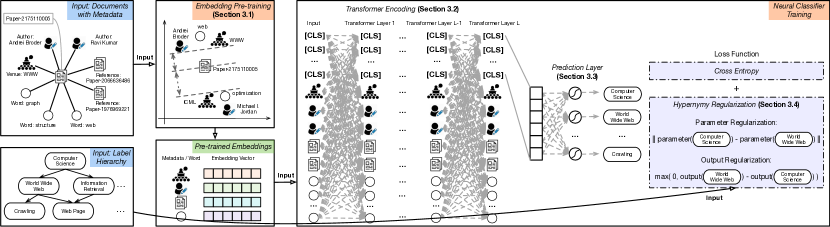
Figure 2. Overview of the MATCH framework.

2. Problem Definition

We study the problem of multi-label text classification. Traditionally, this problem is formalized as using only the text information of documents as the input for inferring their labels (Liu et al., 2017; You et al., 2019; Chang et al., 2020). Here text refers to all free-text fields of a document (e.g., the title and abstract of a scientific publication).

However, the metadata of documents and the hierarchy of labels are usually also available in real-world applications. Take the academic publication in Figure 1 as an example, the metadata of one document includes its authors (e.g., “Samantha K Brooks”), published venue (e.g., “Lancet”), and referenced papers. The label hierarchy is organized based on the fine-grained levels of research topics, such as “Diseases”, “Infections”, and “Eye Infections”.

Formally, we can represent the text information of a document $d$ as a single word sequence $\mathcal{W}_{d}=w_{1}w_{2}\cdots w_{N}$ concatenated from all its text fields, and all its metadata as a set $\mathcal{M}_{d}=\{m_{1},m_{2},\cdots,m_{M}\}$. The label hierarchy can be represented as a tree or a directed acyclic graph (DAG) that specifies the hypernym-hyponym relationships between labels. In both cases, the label hierarchy can be characterized by a mapping $\Phi:\mathcal{L}\rightarrow 2^{\mathcal{L}}$, where $\Phi(l)$ is the set of parent labels of $l\in\mathcal{L}$. If $l$ does not have any parent in $\mathcal{L}$, i.e., $l$ is the root of a tree, we set $\Phi(l)=\emptyset$. We formalize the problem of the metadata-aware text classification with a label hierarchy as follows:

Problem 1.

Given a training corpus $\mathcal{D}=\{d_{1},...,d_{|\mathcal{D}|}\}$, the label space $\mathcal{L}$ and its hierarchy $\Phi$, where each document $d$ is associated with its text information $\mathcal{W}_{d}$, metadata $\mathcal{M}_{d}$, and labels $\mathcal{L}_{d}\subseteq\mathcal{L}$, the objective is to learn a multi-label classifier $f_{\rm class}$ that maps a document to a subset of $\mathcal{L}$.

Different from the conventional multi-label text classification setting (Ji et al., 2008; Liu et al., 2017; You et al., 2019), the task here is both hierarchy- and metadata-aware. There are some previous approaches which have leveraged metadata into text classification problems, ranging from review sentiment analysis (Tang et al., 2015a) and tweet localization (Zhang et al., 2017) to generic classification tasks (Kim et al., 2019; Zhang et al., 2020). However, these studies are all designed for flat text classification.

Along another line of work, some studies try to utilize the label hierarchy via recursive regularization (Gopal and Yang, 2013, 2015; Peng et al., 2018) or hierarchy-aware deep neural models (Wehrmann et al., 2018; Mao et al., 2019; Zhou et al., 2020). However, these approaches are unaware of the metadata signals accompanying each document. The main challenge of our task is then how to simultaneously incorporate the metadata of documents and a hierarchy of labels into a unified learning framework.

3. The MATCH Framework

In this section, we present the MATCH framework for the metadata- and hierarchy-aware multi-label text classification problem. The overall MATCH framework is illustrated in Figure 2, where we use the paper “Graph structure in the Web” as a running example. To incorporate the metadata of documents, MATCH jointly pre-trains the embeddings of metadata, text, and labels into the same latent space, which are further fed into a Transformer model for generating the document representation for prediction. To leverage the hierarchy of labels, MATCH regularizes the parameters and output probabilities of each child label by its parents.

MATCH can be decomposed into four modules: (1) metadata-aware embedding pre-training, (2) Transformer encoding, (3) prediction, and (4) hypernymy regularization.

3.1. Metadata-Aware Embedding Pre-Training

Recently, using pre-trained word embeddings (Mikolov et al., 2013) as the initial input has become a de facto standard for training a neural text classifier (Kim, 2014; Yang et al., 2016; Guo et al., 2019b). However, in our task, it is also required to capture the relationships between text and its metadata, and preferably to have them embedded in the same latent space. To achieve this, we propose a metadata-aware embedding pre-training module to jointly learn their representations by considering several types of proximities between them.

Document & Metadata. To preserve the proximity between a document $d$ and its metadata instances $m\in\mathcal{M}_{d}$ in the joint embedding space, following previous studies on word embedding (Mikolov et al., 2013) and network embedding (Tang et al., 2015c), we define the following conditional probability:

(1) $$p(m|d)=\frac{\exp({\bm{e}}_{m}^{T}{\bm{e}}_{d})}{\sum_{m^{\prime}\in\mathcal{V}_{m}}\exp({\bm{e}}_{m^{\prime}}^{T}{\bm{e}}_{d})},$$

where $\mathcal{V}_{m}$ is the set of metadata instances sharing the same type with $m$ (e.g., if $m$ denotes a venue, then $\mathcal{V}_{m}$ is the set of all venues appearing in the training set); ${\bm{e}}_{m}$ and ${\bm{e}}_{d}$ are metadata and document embedding vectors, respectively.

Given a positive document-metadata pair $(d,m_{+})$, our goal is to maximize the log-likelihood $\log p(m_{+}|d)$ during the embedding learning. To achieve this, we adopt the following margin-based ranking loss:

(2) $$\begin{split}&\max\Big{(}0,\gamma+\log p(m_{-}|d)-\log p(m_{+}|d)\Big{)}\\ \triangleq&\Big{[}\gamma+\log p(m_{-}|d)-\log p(m_{+}|d)\Big{]}_{+}.\end{split}$$

Here, $m_{-}$ is a negative metadata context of document $d$; $\gamma>0$ is a hyperparameter indicating the expected margin between a positive pair $(d,m_{+})$ and a negative pair $(d,m_{-})$. Based on the definition of $p(m|d)$ in Eq. (1), we have

(3) $$\begin{split}&\gamma+\log p(m_{-}|d)-\log p(m_{+}|d)\\ =\ &\gamma+\log\frac{p(m_{-}|d)}{p(m_{+}|d)}\\ =\ &\gamma+\log\frac{\exp({\bm{e}}_{m_{-}}^{T}{\bm{e}}_{d})/\big{(}\sum_{m^{\prime}\in\mathcal{V}_{m}}\exp({\bm{e}}_{m^{\prime}}^{T}{\bm{e}}_{d})\big{)}}{\exp({\bm{e}}_{m_{+}}^{T}{\bm{e}}_{d})/\big{(}\sum_{m^{\prime}\in\mathcal{V}_{m}}\exp({\bm{e}}_{m^{\prime}}^{T}{\bm{e}}_{d})\big{)}}\\ =\ &\gamma+\log\frac{\exp({\bm{e}}_{m_{-}}^{T}{\bm{e}}_{d})}{\exp({\bm{e}}_{m_{+}}^{T}{\bm{e}}_{d})}\\ =\ &\gamma+{\bm{e}}_{m_{-}}^{T}{\bm{e}}_{d}-{\bm{e}}_{m_{+}}^{T}{\bm{e}}_{d}.\end{split}$$

Therefore, the objective function of document-metadata proximity can be defined as follows.

(4) $$\mathcal{J}_{\rm DM}=\sum_{d\in\mathcal{D}}\sum_{m_{+}\in\mathcal{M}_{d}}\sum_{m_{-}\in\mathcal{V}_{m}\backslash\{m_{+}\}}\Big{[}\gamma+{\bm{e}}_{m_{-}}^{T}{\bm{e}}_{d}-{\bm{e}}_{m_{+}}^{T}{\bm{e}}_{d}\Big{]}_{+}.$$

Document & Label. We have label information of each document in the training set. Therefore, the embedding pre-training step can be designed as a supervised process by incorporating those document-label relationships. Specifically, a document $d$ should be closer to its relevant labels $l_{+}$ than to its irrelevant labels $l_{-}$. To encourage this, we can define the conditional probability $p(l|d)$ in a form similar to Eq. (1). Then, following the derivation above, the objective of document-label proximity is

(5) $$\mathcal{J}_{\rm DL}=\sum_{d\in\mathcal{D}}\sum_{l_{+}\in\mathcal{L}_{d}}\sum_{l_{-}\in\mathcal{L}\backslash\{l_{+}\}}\Big{[}\gamma+{\bm{e}}_{l_{-}}^{T}{\bm{e}}_{d}-{\bm{e}}_{l_{+}}^{T}{\bm{e}}_{d}\Big{]}_{+}.$$

Document & Word. The document embedding ${\bm{e}}_{d}$ can be considered as the representation of the theme of $d$. Given a theme, authors write down words that are coherent with the meaning of the entire text. To encourage such coherence, we employ the following objective:

(6) $$\mathcal{J}_{\rm DW}=\sum_{d\in\mathcal{D}}\sum_{w_{+}\in\mathcal{W}_{d}}\sum_{w_{-}\in\mathcal{W}\backslash\{w_{+}\}}\Big{[}\gamma+{\bm{e}}_{w_{-}}^{T}{\bm{e}}_{d}-{\bm{e}}_{w_{+}}^{T}{\bm{e}}_{d}\Big{]}_{+},$$

where $\mathcal{W}_{d}$ is the text sequence of document $d$ and $\mathcal{W}$ is the whole word vocabulary.

Word & Context. Given a text sequence $\mathcal{W}_{d}=w_{1}w_{2}\cdots w_{N}$, the semantic of a word $w_{i}$ depends on not only the document theme but also its surrounding words in the local context window $\mathcal{C}(w_{i})=\{w_{i+j}|-x\leq j\leq x,j\neq 0\}$, where $x$ is the window size. Following (Mikolov et al., 2013), we assume each word has a center word embedding ${\bm{e}}_{w}$ and a context word embedding ${\bm{c}}_{w}$. To encourage the closeness between a word and its local context, the following objective can be proposed.

(7) $$\mathcal{J}_{\rm WW}=\sum_{d\in\mathcal{D}}\sum_{w_{+}\in\mathcal{W}_{d}}\sum_{w_{-}\in\mathcal{W}\backslash\{w_{+}\}}\sum_{w\in\mathcal{C}(w_{+})}\Big{[}\gamma+{\bm{e}}_{w_{-}}^{T}{\bm{c}}_{w}-{\bm{e}}_{w_{+}}^{T}{\bm{c}}_{w}\Big{]}_{+}.$$

Given the objective of each type of relationship, our embedding pre-training module can be formulated as a joint optimization problem as follows.

(8) $$\begin{gathered}\min_{\{{\bm{e}}_{d}\},\{{\bm{e}}_{m}\},\{{\bm{e}}_{l}\},\{{\bm{e}}_{w}\},\{{\bm{c}}_{w}\}}\mathcal{J}_{\rm embedding}=\mathcal{J}_{\rm DM}+\mathcal{J}_{\rm DL}+\mathcal{J}_{\rm DW}+\mathcal{J}_{\rm WW},\\ \text{s.t.\ \ \ }||{\bm{e}}_{d}||_{2}=||{\bm{e}}_{m}||_{2}=||{\bm{e}}_{l}||_{2}=||{\bm{e}}_{w}||_{2}=||{\bm{c}}_{w}||_{2}=1.\end{gathered}$$

We use the L2-norm constraints to control the scale of embedding vectors. These constraints are common when the margin-based ranking loss is used (Bordes et al., 2013; Ren et al., 2017). Without these constraints, the gap between positive and negative pairs (e.g., ${\bm{e}}_{m_{-}}^{T}{\bm{e}}_{d}-{\bm{e}}_{m_{+}}^{T}{\bm{e}}_{d}$) can approach $-\infty$ when $||{\bm{e}}_{d}||_{2}$ becomes arbitrarily large, which makes the optimization problem trivial.

Optimization. The overall objective consists of four parts (i.e., $\mathcal{J}_{\rm DM}$, $\mathcal{J}_{\rm DL}$, $\mathcal{J}_{\rm DW}$ and $\mathcal{J}_{\rm WW}$). To optimize this objective, we adopt the sampling technique introduced in (Tang et al., 2015b) for efficient updating. In each iteration, we alternatively optimize one part (e.g., $\mathcal{J}_{\rm DM}$) by randomly sampling a positive pair (e.g., $(d,m_{+})$) and a corresponding negative pair (e.g., $(d,m_{-})$). Given the two pairs, we can calculate the Euclidean gradient $\nabla^{E}$ of embeddings. Taking $\mathcal{J}_{\rm DM}$ as an example, the gradient vectors are as follows.

(9) $$\begin{gathered}\nabla^{E}\mathcal{J}_{\rm DM}({\bm{e}}_{d})={\bf 1}(\gamma+{\bm{e}}_{m_{-}}^{T}{\bm{e}}_{d}-{\bm{e}}_{m_{+}}^{T}{\bm{e}}_{d}>0)\cdot({\bm{e}}_{m_{-}}-{\bm{e}}_{m_{+}}),\\ \nabla^{E}\mathcal{J}_{\rm DM}({\bm{e}}_{m_{+}})={\bf 1}(\gamma+{\bm{e}}_{m_{-}}^{T}{\bm{e}}_{d}-{\bm{e}}_{m_{+}}^{T}{\bm{e}}_{d}>0)\cdot(-{\bm{e}}_{d}),\\ \nabla^{E}\mathcal{J}_{\rm DM}({\bm{e}}_{m_{-}})={\bf 1}(\gamma+{\bm{e}}_{m_{-}}^{T}{\bm{e}}_{d}-{\bm{e}}_{m_{+}}^{T}{\bm{e}}_{d}>0)\cdot{\bm{e}}_{d},\end{gathered}$$

where ${\bf 1}(\cdot)$ is the indicator function. When optimizing other parts, the Euclidean gradient can be calculated in a similar way.

Recall the constraints of our optimization problem that all embedding vectors need to reside on a sphere. Thus, Euclidean gradient approaches like SGD cannot be directly applied here. Instead, we adopt the Riemannian gradient method (Bonnabel, 2013). Specifically, we calculate the Riemannian gradient $\nabla^{R}$ on a sphere based on the Euclidean gradient $\nabla^{E}$ according to the following equation (Meng et al., 2019):

(10) $$\nabla^{R}\mathcal{J}({\bm{e}})=({\bm{I}}-{\bm{e}}{\bm{e}}^{T})\nabla^{E}\mathcal{J}({\bm{e}}).$$

Then we update the embedding vectors in the following form (Bonnabel, 2013):

(11) $${\bm{e}}^{(t+1)}\leftarrow\frac{{\bm{e}}^{(t)}+\alpha_{t}\nabla^{R}\mathcal{J}({\bm{e}}^{(t)})}{||{\bm{e}}^{(t)}+\alpha_{t}\nabla^{R}\mathcal{J}({\bm{e}}^{(t)})||_{2}},$$

where $\alpha_{t}$ is the learning rate at step $t$.

There are several other ways to jointly embed heterogeneous signals (Tang et al., 2015b; Dong et al., 2017a). For example, PTE (Tang et al., 2015b) constructs three bipartite graphs describing the relationships between labels, words and documents and then embeds these elements into the same latent space. We would like to mention two key differences between our pre-training step and PTE: First, we propose to use a margin-based ranking loss with metadata instances included as well. Second, we formulate the optimization problem in a spherical space and solve it by using the Riemannian gradient method.

3.2. Transformer Layers

Given a document, to facilitate extensive information exchange between text and metadata during document encoding, we adopt the Transformer architecture (Vaswani et al., 2017) as our encoder. Transformer proposes a fully connected attention mechanism to support such exchange between any two tokens in a sequence. Therefore, we concatenate all metadata instances of a document with its word sequence to form the layer input. Moreover, we add [CLS] tokens at the beginning of each input sequence. First proposed in BERT (Devlin et al., 2019), the final state of such special tokens are used as aggregate sequence representation for classification tasks. When the label space is large (e.g., 10K), one [CLS] token (e.g., a 100-dimensional vector) may not be informative enough to predict the relevant labels. Therefore, following (Xun et al., 2020), we put multiple [CLS] tokens [CLS₁], …, [CLS_C] in the input. To summarize, given a document $d$, the layer input ${\bm{H}}$ is

$${\bm{H}}=\big{[}\underbrace{\vphantom{{\bm{e}}_{p_{1}}}{\bm{e}}_{[{\rm CLS}_{1}]};...;{\bm{e}}_{[{\rm CLS}_{C}]}}_{{\rm[CLS]\ tokens}};\ \ \underbrace{\vphantom{{\bm{e}}_{p_{1}}}{\bm{e}}_{m_{1}};...;{\bm{e}}_{m_{M}}}_{{\rm metadata}\ \mathcal{M}_{d}};\ \ \underbrace{\vphantom{{\bm{e}}_{p_{1}}}{\bm{e}}_{w_{1}};...;{\bm{e}}_{w_{N}}}_{{\rm words}\ \mathcal{W}_{d}}\big{]}.$$

Here, ${\bm{H}}\in\mathbb{R}^{\delta\times(C+|\mathcal{M}_{d}|+|\mathcal{W}_{d}|)}$, where $\delta$ is the dimension of the embedding space.

Example 3.1.

(Input Sequence) Suppose we are given the document “Graph structure in the Web” in Figure 2. The input sequence of the Transformer layer will be

“ [CLS₁]  …   [CLS_C]   [Venue_WWW]  [Author_Andrei Broder] [Author_Ravi Kumar] … [Reference_2066636486] [Reference _1976969221]  …   [Word_graph]  [Word_structure]  [Word_in] [Word_the] [Word_web] … ”

Here, the green tokens represent [CLS] symbols; the blue tokens denote metadata instances (i.e., venue, authors and references in this specific example); the orange tokens represent words in the document.

Intuition behind the Metadata-aware Input Sequence. Previous studies (e.g., (Guo et al., 2019b)) have pointed out that, given an input sequence $\mathcal{S}$, Transformer treats $\mathcal{S}$ as a fully connected token graph. For each token $i\in\mathcal{S}$, its context is the entire sequence, and its representation will be updated by aggregating the information from all tokens $j\in\mathcal{S}$. In our case, $\mathcal{S}$ is the union of $\mathcal{M}_{d}$, $\mathcal{W}_{d}$ and [CLS] tokens. Hence, the attention mechanism allows each [CLS] token to aggregate information from all metadata instances and words. Moreover, if we treat each input document as an ego network of the document node $d$ (as shown in Figure 2), our embedding pre-training step essentially captures first-order proximity between $d$ and its neighbors, while the fully connected attention mechanism here describes second-order proximity in $d$’s neighborhood. In other words, our Transformer layer facilitates higher-order interactions among metadata instances and words.

Multi-head Attention. Now we formally introduce the attention mechanism in the Transformer layer. As in (Vaswani et al., 2017), given ${\bm{H}}$, one can use a query vector ${\bm{q}}\in\mathbb{R}^{1\times\delta}$ to select relevant information with attention.

(12) $$\textrm{Attention}({\bm{q}},{\bm{K}},{\bm{V}})=\textrm{Softmax}\Big{(}\frac{{\bm{q}}{\bm{K}}^{T}}{\sqrt{\delta}}\Big{)}{\bm{V}},$$

where ${\bm{K}}={\bm{H}}{\bm{W}}^{K}$ and ${\bm{V}}={\bm{H}}{\bm{W}}^{V}$. Matrices ${\bm{W}}^{K}$ and ${\bm{W}}^{V}$ are parameters to be learned.

Similar to the idea of multiple channels in CNN, Transformer uses multi-head attention to extract more signals from ${\bm{H}}$. Formally,

(13) $$\begin{gathered}{\bm{a}}_{i}=\textrm{Attention}({\bm{q}}{\bm{W}}^{Q}_{i},{\bm{H}}{\bm{W}}^{K}_{i},{\bm{H}}{\bm{W}}^{V}_{i}),\\ \textrm{MultiHeadAtt}({\bm{q}},{\bm{H}})=\big{[}{\bm{a}}_{1}\ ||\ {\bm{a}}_{2}\ ||\ ...\ ||\ {\bm{a}}_{k}\big{]}{\bm{W}}^{O},\end{gathered}$$

where $||$ denotes the concatenation operation. Matrices ${\bm{W}}^{Q}_{i}$, ${\bm{W}}^{K}_{i}$, ${\bm{W}}^{V}_{i}$ and ${\bm{W}}^{O}$ are learnable parameters.

Document Encoding. Using multi-head attention, for each input token $i\in{\bm{H}}$, we update its representation based on its pre-trained embedding ${\bm{e}}_{i}$.

(14) $$\begin{gathered}{\bm{z}}_{i}=\textrm{LayerNorm}\big{(}{\bm{e}}_{i}+\textrm{MultiHeadAtt}({\bm{e}}_{i},{\bm{H}})\big{)},\\ {\bm{h}}_{i}=\textrm{LayerNorm}\big{(}{\bm{z}}_{i}+\textrm{FFN}({\bm{z}}_{i})\big{)}.\end{gathered}$$

Here, $\textrm{LayerNorm}(\cdot)$ is the layer normalization operator (Ba et al., 2016) and $\textrm{FFN}(\cdot)$ is the position-wise feed-forward network (Vaswani et al., 2017). To incorporate position information of the token, we further concatenate its sinusoidal position embedding (Vaswani et al., 2017) with its input embedding ${\bm{e}}_{i}$.

Eq. (14) describes one Transformer layer. As shown in Figure 2, we can stack $L$ Transformer layers, where the output of the $l$-th layer ${\bm{H}}^{(l)}$ is also the input of the $(l+1)$-th layer. ${\bm{H}}^{(0)}$ consists of the pre-trained embeddings, and ${\bm{H}}^{(L)}$ is used for prediction.

3.3. Prediction Layer

After $L$ Transformer layers, we concatenate the final state of all [CLS] tokens to get the final document representation $\widehat{{\bm{h}}}_{d}$.

(15) $$\widehat{{\bm{h}}}_{d}={\bm{h}}^{(L)}_{[{\rm CLS}_{1}]}\ ||\ {\bm{h}}^{(L)}_{[{\rm CLS}_{2}]}\ ||\ ...\ ||\ {\bm{h}}^{(L)}_{[{\rm CLS}_{C}]}.$$

To perform classification, we add a fully connected layer upon the output of Transformer. The final layer is then connected to $|\mathcal{L}|$ sigmoid functions, which correspond to all labels in $\mathcal{L}$. The output of the $l$-th sigmoid function ($\uppi_{dl}$) denotes the probability that document $d$ should be tagged with label $l$. Formally,

(16) $${\bm{\uppi}}_{d}=\textrm{Sigmoid}\big{(}\widehat{{\bm{h}}}_{d}{\bm{W}}^{\Pi}+{\bm{b}}\big{)},$$

where ${\bm{W}}^{\Pi}=[{\bm{w}}_{1},...,{\bm{w}}_{|\mathcal{L}|}]$ and ${\bm{w}}_{l}$ can be viewed as the parameters specific to the $l$-th label.

Given the output probabilities, our model minimizes the binary cross-entropy (BCE) loss by treating the multi-label classification task as $|\mathcal{L}|$ binary classification subtasks.

(17) $$\mathcal{J}_{\rm BCE}=-\sum_{d\in\mathcal{D}}\sum_{l\in\mathcal{L}}\big{(}y_{dl}\log\uppi_{dl}+(1-y_{dl})\log(1-\uppi_{dl})\big{)},$$

where $y_{dl}=1$ means document $d$ has label $l$, and $y_{dl}=0$ otherwise.

3.4. Hypernymy Regularization

In hierarchical text classification, a given label taxonomy contains valuable signals of label intercorrelation, which should be leveraged in the classification process. However, most existing studies ignore the label dependencies in the input taxonomy (Liu et al., 2017; Xun et al., 2019; You et al., 2019).

To incorporate the label hierarchy into MATCH, we propose to regularize each non-root label by its parents. Specifically, the regularization is applied in both the parameter space and the output space. In the parameter space, instead of treating the class-specific parameters ${\bm{w}}_{1},...,{\bm{w}}_{|\mathcal{L}|}$ as independent, we design a regularization mechanism for modeling the dependencies in the prediction layer; In the output space, we enable the interactions between the output probabilities $\uppi_{d1},...,\uppi_{d|\mathcal{L}|}$ in the loss function.

Regularization in the Parameter Space. Similar to (Gopal and Yang, 2013; Peng et al., 2018), we use an L2-norm penalty to enforce the parameters of each label to be similar to its parent.

(18) $$\mathcal{J}_{\rm parameter}=\sum_{l\in\mathcal{L}}\sum_{l^{\prime}\in\Phi(l)}\frac{1}{2}||{\bm{w}}_{l}-{\bm{w}}_{l^{\prime}}||^{2},$$

where $\Phi(l)$ denotes the set of parent labels of $l$. Intuitively, this regularization encourages comparable criteria of categories that are nearby in the hierarchy. For example, judging whether a document can be tagged with “Crawling” should bear similarities with judging whether it is related to its parent label “World Wide Web”.

Regularization in the Output Space. Previous studies on hierarchical regularization (Gopal and Yang, 2013; Peng et al., 2018) only consider the “similarity” between parent and child labels. To be specific, in Eq. (18), the L2-norm is symmetric on the child $l$ and the parent $l^{\prime}$. In other words, even if we swap $l$ and $l^{\prime}$, the regularization term for ${\bm{w}}_{l}$ and ${\bm{w}}_{l^{\prime}}$ remains unchanged. This could be insufficient to capture the asymmetry between parent and child labels. To address this issue, inspired by the distributional inclusion hypothesis (DIH) (Geffet and Dagan, 2005), we propose a novel regularization term to characterize the hypernym-hyponym relationships.

Definition 3.2.

(Distributional Inclusion Hypothesis (Geffet and Dagan, 2005)) If the meaning of a word $w_{1}$ entails another word $w_{2}$, then it is expected that all the typical contexts of $w_{1}$ will also occur with $w_{2}$.

According to this definition, $w_{2}$ is viewed as a hypernym (i.e., parent) and $w_{1}$ is viewed as a hyponym (i.e., child). Note that one can interpret DIH in various ways depending on how “contexts” are defined. For example, if “contexts” are defined as documents (Shi et al., 2019), then DIH states that: if a word (e.g., “Crawling”) appears in a document, then its parent (e.g., “World Wide Web”) is also expected to be in that document. In contrast, if “contexts” are defined based on the local context window (i.e., the previous and the latter words in a sequence) (Shwartz et al., 2017), then DIH becomes: if a context word $c$ occurs $n$ times in the context window of a child $w_{1}$, then it is expected to occur no less than $n$ times in the context window of its parent $w_{2}$. DIH is a classic tool in constructing topic taxonomies (Shi et al., 2019; Shen et al., 2018), which motivates us to propose the following DIH-based regularization.

In the document classification task, the hypernym $w_{2}$ and hyponym $w_{1}$ become the parent label $l^{\prime}$ and child label $l$, respectively. We define the “contexts” of a label $l$ to be the documents tagged with $l$. From this perspective, DIH can be interpreted as: if a document $d$ belongs to the child class $l$ with probability $\uppi_{dl}$, then it should belong to the parent class $l^{\prime}$ with probability no less than $\uppi_{dl}$. For example, if there is a 50% chance a paper will be labeled with “Crawling”, then the chance to tag this paper with “World Wide Web” should be at least 50%. Formally, the regularization term is defined as

(19) $$\mathcal{J}_{\rm output}=\sum_{d\in\mathcal{D}}\sum_{l\in\mathcal{L}}\sum_{l^{\prime}\in\Phi(l)}\max\big{(}0,\uppi_{dl}-\uppi_{dl^{\prime}}\big{)}.$$

Unlike the parameter regularization, Eq. (19) is asymmetric: $\uppi_{dl}>\uppi_{dl^{\prime}}$ will incur a penalty, but $\uppi_{dl^{\prime}}>\uppi_{dl}$ will not.

Based on the BCE loss and the two proposed regularization terms, we use the following objective to learn the parameters of our neural architecture:

(20) $$\min\mathcal{J}=\mathcal{J}_{\rm BCE}+\lambda_{1}\mathcal{J}_{\rm parameter}+\lambda_{2}\mathcal{J}_{\rm output},$$

where $\lambda_{1}$ and $\lambda_{2}$ are two hyperparameters.

4. Experiments

4.1. Setup

Datasets. We evaluate our method on two large-scale datasets.

• MAG-CS (Wang et al., 2020). The Microsoft Academic Graph (MAG) has a web-scale collection of scientific papers covering a broad spectrum of academic disciplines. As of February 2021, it has more than 251 million academic papers and over 729 thousand labels. MAG has also performed author name disambiguation and represented each author with a unique ID. Based on MAG, we construct a dataset focusing on the computer science domain. Specifically, we select papers published at 105 top CS conferences from 1990 to 2020. MAG has a high-quality label taxonomy constructed semi-automatically (Shen et al., 2018). For each selected paper, we remove its labels that are not in the CS domain (i.e., not descendants of “Computer Science” in the taxonomy). We also remove the root label “Computer Science” which is trivial to predict. After paper selection and label filtering, we obtain 705,407 documents and 15,809 labels. We refer to this dataset as MAG-CS.

• PubMed (Lu, 2011). PubMed comprises more than 30 million articles (abstracts) of biomedical literature from MEDLINE, life science journals, and online books. In our experiment, we focus on papers published in 150 top journals in medicine from 2010 to 2020. For each paper selected from PubMed, we find it in MAG so that we can obtain its disambiguated author, venue, and reference information. Each PubMed paper is tagged with related MeSH terms (Coletti and Bleich, 2001), which are viewed as labels in our task. In the MeSH hierarchy, we focus on the first 8 top-level categories (i.e., A–H). After selection, we have 898,546 documents and 17,693 labels.

For both datasets, we use 80% of the documents for training, 10% for validation, and 10% for testing. The text information of each document is its title and abstract; the metadata information includes authors, venue, and references. Table 1 summarizes the statistics of the two datasets.

Table 1. Dataset statistics.

	MAG-CS (Sinha et al., 2015)	PubMed (Lu, 2011)
# Training Docs	564,340	718,837
# Validation Docs	70,534	89,855
# Testing Docs	70,533	89,854
# Labels	15,809	17,963
# Labels / Doc	5.60	7.78
Vocabulary Size	425,316	776,975
# Words / Doc	126.33	198.97
# Authors	818,927	2,201,919
# Venues	105	150
# Paper-Author Edges	2,274,546	5,989,142
# Paper-Venue Edges	705,407	898,546
# Paper-Paper Edges	1,518,466	4,455,702
# Edges in Taxonomy	27,288	22,842
# Layers of Taxonomy	6	15

Table 2. Performance of compared algorithms on MAG-CS. *: significantly worse than MATCH (p-value $<0.05$). **: significantly worse than MATCH (p-value $<0.01$).

Algorithms	P@1$=$NDCG@1	P@3	P@5	NDCG@3	NDCG@5
XML-CNN (Liu et al., 2017)	0.8656 $\pm$ 0.0006**	0.7028 $\pm$ 0.0010**	0.5756 $\pm$ 0.0010**	0.7842 $\pm$ 0.0009**	0.7407 $\pm$ 0.0009**
MeSHProbeNet (Xun et al., 2019)	0.8738 $\pm$ 0.0016**	0.7219 $\pm$ 0.0059**	0.5927 $\pm$ 0.0075**	0.8020 $\pm$ 0.0048**	0.7588 $\pm$ 0.0067**
AttentionXML (You et al., 2019)	0.9035 $\pm$ 0.0009**	0.7682 $\pm$ 0.0017**	0.6441 $\pm$ 0.0020	0.8489 $\pm$ 0.0016**	0.8145 $\pm$ 0.0020**
Star-Transformer (Guo et al., 2019b)	0.8569 $\pm$ 0.0011**	0.7089 $\pm$ 0.0010**	0.5853 $\pm$ 0.0011**	0.7876 $\pm$ 0.0008**	0.7486 $\pm$ 0.0011**
BERTXML (Xun et al., 2020)	0.9011 $\pm$ 0.0027**	0.7532 $\pm$ 0.0015**	0.6238 $\pm$ 0.0020*	0.8355 $\pm$ 0.0025**	0.7954 $\pm$ 0.0024**
Transformer (Vaswani et al., 2017)	0.8805 $\pm$ 0.0007**	0.7327 $\pm$ 0.0006**	0.6024 $\pm$ 0.0010**	0.8129 $\pm$ 0.0008**	0.7703 $\pm$ 0.0010**
MATCH-NoMetadata	0.9041 $\pm$ 0.0012**	0.7640 $\pm$ 0.0010*	0.6376 $\pm$ 0.0002*	0.8440 $\pm$ 0.0012**	0.8068 $\pm$ 0.0005**
MATCH-NoHierarchy	0.9114 $\pm$ 0.0014*	0.7634 $\pm$ 0.0012**	0.6312 $\pm$ 0.0013**	0.8486 $\pm$ 0.0006**	0.8076 $\pm$ 0.0009**
MATCH	0.9190 $\pm$ 0.0012	0.7763 $\pm$ 0.0023	0.6457 $\pm$ 0.0030	0.8610 $\pm$ 0.0022	0.8223 $\pm$ 0.0030

Table 3. Performance of compared algorithms on PubMed. *: significantly worse than MATCH (p-value $<0.05$). **: significantly worse than MATCH (p-value $<0.01$).

Algorithms	P@1$=$NDCG@1	P@3	P@5	NDCG@3	NDCG@5
XML-CNN (Liu et al., 2017)	0.9084 $\pm$ 0.0004**	0.7182 $\pm$ 0.0007**	0.5857 $\pm$ 0.0004**	0.7790 $\pm$ 0.0007**	0.7075 $\pm$ 0.0005**
MeSHProbeNet (Xun et al., 2019)	0.9135 $\pm$ 0.0021	0.7224 $\pm$ 0.0066*	0.5878 $\pm$ 0.0070*	0.7836 $\pm$ 0.0057*	0.7109 $\pm$ 0.0065*
AttentionXML (You et al., 2019)	0.9125 $\pm$ 0.0003*	0.7414 $\pm$ 0.0017*	0.6169 $\pm$ 0.0016	0.7979 $\pm$ 0.0013*	0.7341 $\pm$ 0.0013
Star-Transformer (Guo et al., 2019b)	0.8962 $\pm$ 0.0023**	0.6990 $\pm$ 0.0014**	0.5641 $\pm$ 0.0008**	0.7612 $\pm$ 0.0015**	0.6869 $\pm$ 0.0011**
BERTXML (Xun et al., 2020)	0.9144 $\pm$ 0.0014*	0.7362 $\pm$ 0.0046*	0.6032 $\pm$ 0.0050*	0.7949 $\pm$ 0.0038*	0.7247 $\pm$ 0.0045*
Transformer (Vaswani et al., 2017)	0.8971 $\pm$ 0.0050*	0.7299 $\pm$ 0.0029**	0.6003 $\pm$ 0.0018**	0.7867 $\pm$ 0.0034**	0.7178 $\pm$ 0.0027**
MATCH-NoMetadata	0.9153 $\pm$ 0.0022	0.7408 $\pm$ 0.0035*	0.6080 $\pm$ 0.0036**	0.7987 $\pm$ 0.0031*	0.7290 $\pm$ 0.0034*
MATCH-NoHierarchy	0.9151 $\pm$ 0.0022	0.7425 $\pm$ 0.0041	0.6104 $\pm$ 0.0047	0.8001 $\pm$ 0.0037	0.7310 $\pm$ 0.0044
MATCH	0.9168 $\pm$ 0.0013	0.7511 $\pm$ 0.0029	0.6199 $\pm$ 0.0029	0.8072 $\pm$ 0.0027	0.7395 $\pm$ 0.0029

Compared Methods. We compare the following approaches including both extreme multi-label text classification methods as well as Transformer-based models.

• XML-CNN (Liu et al., 2017) is an extreme multi-label text classification method based on convolutional neural networks. It modifies Kim-CNN (Kim, 2014) by introducing a dynamic max-pooling scheme, a bottleneck layer, and the BCE loss.

• MeSHProbeNet (Xun et al., 2019) was originally designed for tagging biomedical documents with relevant MeSH terms. It can also be applied to a general multi-label text classification setting. MeSHProbeNet models text sequences using recurrent neural networks and uses multiple MeSH “probes” to extract information from RNN hidden states.

• AttentionXML (You et al., 2019) is an extreme multi-label text classification method built upon a bidirectional RNN layer and a label-aware attention layer. It also leverages hierarchical label trees to recursively warm-start the model.

• Transformer (Vaswani et al., 2017) is a fully connected attention-based model. Since we have massive training data in both datasets, we train a Transformer encoder from scratch using text classification as the downstream task. Following (Liu et al., 2019), after getting the output representation of all tokens, we average them to get document representation and pass it through a fully connected layer to perform multi-label classification.

• Star-Transformer (Guo et al., 2019b) simplifies Transformer by sparsifying fully connected attention to a star-shaped structure. This sparsification leads to performance improvement on moderately sized training sets.

• BERTXML (Xun et al., 2020) is a model inspired by BERT (Devlin et al., 2019). It utilizes a multi-layer Transformer structure and adds multiple [CLS] symbols in front of the input sequence to obtain the aggregate sequence representation.

• MATCH is our proposed model with metadata-aware pre-training, metadata-aware Transformer encoding, and hypernymy regularization.

• MATCH-NoMetadata is an ablation version of the full MATCH model without using metadata information in both pre-training and Transformer layers.

• MATCH-NoHierarchy is an ablation version of the full MATCH model without hypernymy regularization.

Implementation and Hyperparameters. For all compared algorithms, the embedding dimension $\delta$ is 100. We use GloVe.6B.100d (Pennington et al., 2014) as initialized word embeddings for all models except MATCH and MATCH-NoHierarchy (whose initialized embeddings are learned from metadata-aware pre-training). The training process is performed using Adam (Kingma and Ba, 2014) with a batch size of 256. The baselines are implemented in two GitHub repositories . We directly use their default parameter settings when running the baselines.

For our MATCH framework, we set the margin of embedding pre-training $\gamma=0.3$, number of attention heads $k=2$, number of [CLS] tokens $C=8$, number of Transformer layers $L=3$, and the dropout rate to be 0.1.

(a) MAG-CS

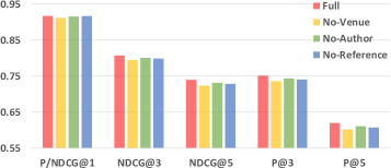
(b) PubMed

Figure 3. Ablation analysis of metadata.

Evaluation Metrics. In many multi-label classification datasets, even if the label space is large, each document only has very few relevant labels. For example, in Table 1, we show that both MAG-CS and PubMed have over 15K labels in total, but each document has 5.60 and 7.78 labels on average, respectively. Considering the sparsity of labels, a short-ranked list of potentially relevant labels for each testing document is commonly used to represent classification quality. Following previous studies on extreme multi-label text classification (Liu et al., 2017; You et al., 2019; Xun et al., 2020), we adopt two rank-based metrics: the precision at top $k$ (P@$k$) and the normalized Discounted Cumulative Gain at top $k$ (NDCG@$k$), where $k=1,3,5$. For a document $d$, let ${\bm{y}}_{d}\in\{0,1\}^{|\mathcal{L}|}$ be its ground truth label vector and ${\rm rank}(i)$ be the index of the $i$-th highest predicted label according to the output probability ${\bm{\uppi}}_{d}$. Then, P@$k$ and NDCG@$k$ are formally defined as

(21) $$\begin{gathered}{\rm P@}k=\frac{1}{k}\sum_{i=1}^{k}y_{d,{\rm rank}(i)}.\\ {\rm DCG@}k=\sum_{i=1}^{k}\frac{y_{d,{\rm rank}(i)}}{\log(i+1)},\\ {\rm NDCG@}k=\frac{{\rm DCG@}k}{\sum_{i=1}^{\min(k,||{\bm{y}}_{d}||_{0})}\frac{1}{\log(i+1)}}.\end{gathered}$$

It is easy to show that ${\rm P@}1\equiv{\rm NDCG@}1$ if each document has at least one true label.

4.2. Performance Comparison

Tables 2 and 3 demonstrate the performance of compared algorithms on MAG-CS and PubMed, respectively. We run each experiment three times with the mean and standard deviation reported. To measure statistical significance, we conduct a two-tailed paired t-test to compare MATCH and each baseline. The significance level of each result is marked in the tables.

On MAG-CS, as we can observe from Table 2: (1) MATCH consistently outperforms all baseline approaches. In almost all cases, the gap is statistically significant, with only one exception where P@5 of AttentionXML is close to that of MATCH. (2) MATCH also significantly outperforms the two ablation versions MATCH-NoMetadata and MATCH-NoHierarchy. This observation validates our claim that both metadata and hierarchy signals are beneficial to the classification performance. (3) Although Star-Transformer is shown to be more effective and efficient than the standard Transformer for modestly sized training sets (Guo et al., 2019b), its simplified structure is less capable of fitting large-scale training sets. The comparison between Star-Transformer and Transformer in Table 2 shows that MAG-CS is large enough to train a fully connected Transformer architecture from scratch. (4) The standard Transformer outperforms two dedicated multi-label text classification approaches, XML-CNN and MeSHProbeNet, which demonstrates the advantage of Transformer’s fully connected attention mechanism over CNN and RNN architectures on MAG-CS. Built upon Transformer, MATCH can also outperform XML-CNN and MeSHProbeNet, even without metadata information.

On PubMed, MATCH still performs the best among all compared approaches, and most observations from Table 2 hold in Table 3. However, we would like to emphasize one unique finding: the contribution of hypernymy regularization is no longer significant on PubMed. To be specific, on MAG-CS, MATCH has an average absolute improvement of 1.2% on the five metrics in comparison with MATCH-NoHierarchy; on PubMed, the improvement becomes 0.7%. We believe this is due to different labeling patterns on the two datasets. As we can see, the effect of hypernymy regularization depends on the correlation between parent and child labels. In fact, when a document is tagged with a child label, we expect it will be labeled with its parents as well. However, this assumption is not often correct on PubMed as sometimes human annotators will only select those more specific categories to annotate the document. On MAG-CS, the assumption holds in more cases because each document is guaranteed to have at least one layer-1 label.

4.3. Effect of Metadata

In both datasets, we have three types of metadata information: authors, venue, and references. To check whether each of them is useful, we conduct an ablation analysis to study the performance change when MATCH is blind to one type of metadata. To do this, we create three ablation versions of MATCH: No-Author, No-Venue, and No-Reference. For No-Author, we remove author information from the input metadata $\mathcal{M}_{d}$ of each document $d$. Similarly, we can define No-Venue and No-Reference.

Figure 3 depicts the comparisons between MATCH and its three ablations. We observe that: (1) The full MATCH model outperforms No-Author, No-Venue, and No-Reference in most cases, indicating that all three types of metadata play a positive role in the classification process. (2) Among the three ablation versions, No-Venue consistently performs the worst. In other words, venue information has the largest contribution. In fact, when $k=1$, the contribution of authors and references to P/NDCG@$k$ is quite subtle, while venue signals have an evident offering. To explain this, we recall the hypernymy regularization inspired by DIH. We expect the predicted probability of a parent category to be no less than that of its children. Thus, the more general a label is, the higher probability it is expected to have. That being said, layer-1 categories are assumed to be ranked higher in the prediction list. Therefore, as strong indicators of coarse-grained classes (e.g., “Data Mining” and “Natural Language Processing”), venues are expected to be most helpful to predict the higher-ranked labels. Since venues already give enough hints, overlooking authors or references will not lead to a visible performance drop when $k=1$. (3) As $k$ increases, the contribution of authors and references becomes larger. For example, on PubMed, the difference of P@1 between Full and No-Author is 0.1%, but the difference of P@5 becomes 0.9%. This is because venues are less beneficial to the prediction of fine-grained categories (e.g., “Named Entity Recognition” and “Entity Linking”), but authors and references may provide such signals.

4.4. Effect of Embedding Pre-Training

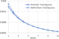
(a) MAG-CS, Training Loss

(b) MAG-CS, Validation NDCG@$k$

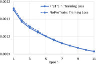
(c) PubMed, Training Loss

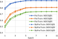
(d) PubMed, Validation NDCG@$k$

Figure 4. Performance of MATCH during the training process with and without metadata-aware embedding pre-training.

We have shown the positive contribution of leveraging different types of metadata in MATCH, which is a combined effect of metadata-aware embedding pre-training and metadata-aware Transformer encoding. Now we would like to show the advantages of embedding pre-training alone. To facilitate this, we create another ablation version, MATCH-NoPreTrain, which bypasses metadata-aware embedding pre-training and directly uses GloVe.6B.100d as initialized embeddings of our neural classifier.

Figure 4 demonstrates the performance of MATCH and MATCH-NoPreTrain during the training process. The x-axis represents training epochs. In Figures 4(a) and (c), the y-axis is the average training loss of the last 100 batches in epoch $x$. In Figures 4(b) and (d), the y-axis represents NDCG@$k$ ($k=1,3,5$) of the trained classifier on the validation set after epoch $x$. The full model is denoted by solid lines and NoPreTrain is denoted by dashed lines. We can observe that: (1) In earlier epochs, the full model achieves evidently higher NDCG@$k$ scores and lower training loss than NoPreTrain, indicating that embedding pre-training provides a warm start to neural classifier training. This is intuitive because the embeddings of metadata instances and words unseen in GloVe.6B.100d need to be randomly initialized in MATCH-NoPreTrain. As training proceeds, the performance of NoPreTrain becomes on par with that of the full model, which means metadata-aware pre-training cannot significantly boost the final NDCG@$k$ scores. The reason could be that our Transformer-based encoder already captures higher-order information than the pre-training step does (as mentioned in Section 3.2), which makes up for the cold start caused by random initialization. (2) The NDCG@$k$ curves of both models converge before epoch 11. On MAG-CS, the full model achieves its best NDCG@1 at epoch 7 while NoPreTrain gets the highest NDCG@1 at epoch 10. On PubMed, the peak NDCG@1 scores of MATCH and MATCH-NoPreTrain are at epoch 7 and epoch 8, respectively. To summarize, on both datasets, the full model converges earlier than NoPreTrain in terms of precision on the validation set. In other words, metadata-aware pre-training increases the speed of model convergence in MATCH.

4.5. Case Study

Table 4. Case Study on MAG-CS. Orange: Incorrect predictions. Blue: Correct predictions when utilizing metadata, and the corresponding signals. Green: Correct predictions when utilizing the hierarchy, and the corresponding signals.

Case 1: Effect of Metadata
Title: Improving Text Categorization Methods for Event Tracking
Venue: SIGIR (2000)
Authors: Yiming Yang, Tom Ault, Thomas Pierce, Charles W. Lattimer
Abstract: Automated tracking of events from chronologically ordered document streams is a new challenge for statistical text classification. Existing learning techniques must be adapted or improved in order to effectively handle difficult situations where the number of positive training instances per event is extremely small, the majority of training documents are unlabelled, and most of the events have a short duration in time. We adapted several supervised text categorization methods, specifically several new variants of the k-Nearest Neighbor (kNN) algorithm …
Ground Truth Labels: Data Mining, Machine Learning, Information Retrieval, K Nearest Neighbors Algorithm, Pattern Recognition
Top-5 Predictions of Transformer: K Nearest Neighbors Algorithm (✓), Data Mining (✓), Pattern Recognition (✓), Machine Learning (✓), Nearest Neighbor Search (✗)
Top-5 Predictions of MATCH-NoHierarchy: K Nearest Neighbors Algorithm (✓), Data Mining (✓), Pattern Recognition (✓), Information Retrieval (✓), Machine Learning (✓)
Top-5 Predictions of MATCH: K Nearest Neighbors Algorithm (✓), Data Mining (✓), Information Retrieval (✓), Pattern Recognition (✓), Machine Learning (✓)
Case 2: Effect of Hierarchy
Title: Automatic Derivation of a Phoneme Set with Tone Information for Chinese Speech Recognition Based on Mutual Information Criterion
Venue: ICASSP (2006)
Abstract: An appropriate approach to model tone information is helpful for building Chinese large vocabulary continuous speech recognition system. We propose to derive an efficient phoneme set of tone-dependent sub-word units to build a recognition system, by iteratively merging a pair of tone-dependent units according to the principle of minimal loss of the mutual information. The mutual information is measured between the word tokens and their phoneme transcriptions in a training text corpus, based on the system lexical and language model. …
Hypernymy Information: parents( Language Model ) $=$ { Artificial Intelligence, Speech Recognition, Natural Language Processing }
Ground Truth Labels: Vocabulary, Homophone, Natural Language, Audio Mining, Speech Recognition, Natural Language Processing, Word Error Rate, Language Model, Text Corpus, Pattern Recognition, Mutual Information
Top-5 Predictions of Transformer: Speech Recognition (✓), Discriminative Model (✗), Language Model (✓), Mutual Information (✓), Vocabulary (✓)
Top-5 Predictions of MATCH-NoHierarchy: Mutual Information (✓), Speech Recognition (✓), Vocabulary (✓), Discriminative Model (✗), Language Model (✓)
Top-5 Predictions of MATCH: Text Corpus (✓), Speech Recognition (✓), Language Model (✓), Mutual Information (✓), Natural Language Processing (✓)
Case 3: An Error of MATCH
Title: The Winograd Schema Challenge and Reasoning about Correlation
Venue: AAAI (2015)
Abstract: The Winograd Schema Challenge is an alternative to the Turing Test that may provide a more meaningful measure of machine intelligence. It poses a set of coreference resolution problems that cannot be solved without human-like reasoning. In this paper, we take the view that the solution to such problems lies in establishing discourse coherence. Specifically, we examine two types of rhetorical relations that can be used to establish discourse coherence: positive and negative correlation. We introduce a framework for reasoning about correlation …
Ground Truth Labels: Coreference, Artificial Intelligence, Natural Language Processing, Winograd Schema Challenge, Turing Test
Top-5 Predictions of Transformer: Turing Test (✓), Winograd Schema Challenge (✓), Natural Language Processing (✓), Coreference (✓), Artificial Intelligence (✓)
Top-5 Predictions of MATCH-NoHierarchy: Winograd Schema Challenge (✓), Turing Test (✓), Coreference (✓), Machine Learning (✗), Artificial Intelligence (✓)
Top-5 Predictions of MATCH: Turing Test (✓), Winograd Schema Challenge (✓), Coreference (✓), Machine Learning (✗), Artificial Intelligence (✓)

We now conduct case studies to qualitatively understand the effects of incorporating metadata and the label hierarchy. Table 4 compares the full MATCH model with MATCH-NoHierarchy and Transformer on the predictions of three MAG-CS papers. For each paper, we show its text, (part of) metadata/hierarchy information, ground truth labels as well as top-5 predicted labels of the three compared approaches. Recall that MATCH-NoHierarchy does not use any label hierarchy information, and Transformer is unaware of both metadata and the hierarchy.

In Case 1, the paper has a ground truth label “Information Retrieval”. Although the term “retrieval” does not explicitly appear in the title and abstract, metadata signals (especially the venue “SIGIR” and one of the authors “Yiming Yang”) successfully indicate the paper’s relevance to “Information Retrieval”. However, Transformer fails to predict “Information Retrieval” in its top-5 choices as it is blind to metadata. Instead, it makes a wrong prediction “Nearest Neighbor Search”. In contrast, both MATCH and MATCH-NoHierarchy can observe metadata information, thus both of them correctly pick “Information Retrieval”.

In Case 2, the paper is related to a fine-grained topic “Language Model” and a broader category “Natural Language Processing”. As the paper mentions “language model” and related terms in its abstract, the three compared approaches all include “Language Model” correctly in their top-5 choices. According to the hypernymy information, we can see three parent categories of “Language Model”, which are “Artificial Intelligence”, “Speech Recognition”, and “Natural Language Processing”. The last two are in the ground truth labels of this paper. Unlike “Speech Recognition” which can be easily inferred from the title, “Natural Language Processing” can be neither found in the text nor indicated by the venue. Therefore, “Natural Language Processing” is missed by Transformer and MATCH-NoHierarchy. In contrast, by observing the hierarchy information, MATCH successfully picks “Natural Language Processing” in its top-5 predictions.

Case 1 and Case 2 reflect the benefit of considering metadata and the hierarchy, respectively. However, in a few cases, such additional signals may also confuse our model. We show an error made by MATCH in Case 3. The paper is about the Winograd Schema Challenge. Transformer successfully predicts all ground truth labels in its top-5 choices. However, both MATCH-NoHierarchy and MATCH give a wrong prediction “Machine Learning”, probably because the paper is published at AAAI which has many machine learning studies. In fact, the paper is purely based on formal logical reasoning and has no machine learning related component. This case implies an interesting future direction on how to automatically select topic-indicative metadata instances to help classification.

5. Related Work

Multi-label Text Classification. Traditional multi-label text classification approaches mainly use bag-of-words representations and can be divided into three categories: (1) One-vs-all methods (Babbar and Schölkopf, 2017; Yen et al., 2016; Yen et al., 2017) exploit data sparsity to learn a classifier for each label independently. (2) Tree-based approaches (Jain et al., 2016; Prabhu and Varma, 2014; Prabhu et al., 2018; Siblini et al., 2018) recursively partition the feature space at each non-leaf node and learn a classifier focusing on only a few active labels at each leaf node. (Note that they are hierarchically partitioning the feature space instead of the label space, thus cannot be viewed as conventional hierarchical text classification methods.) (3) Embedding-based approaches (Bhatia et al., 2015; Guo et al., 2019a; Chen and Lin, 2012; Tagami, 2017) represent labels as low-dimensional vectors and perform classification by finding the nearest label neighbors of each document in the latent space. Recently, deep learning based methods leverage deep neural architectures to learn better text representations. For example, Liu et al. (Liu et al., 2017) propose a convolutional neural network with dynamic pooling and a hidden bottleneck layer for text encoding. Nam et al. (Nam et al., 2017) leverage recurrent neural networks to encode text sequences and generate predicted labels sequentially. You et al. (You et al., 2019) adopt attention models to capture the most relevant parts of the input text to each label. Chang et al. (Chang et al., 2020) utilize pre-trained Transformers as neural matchers to perform classification. There are also multi-label classifiers specifically designed for biomedical literature such as DeepMeSH (Peng et al., 2016), MeSHProbeNet (Xun et al., 2019), and FullMeSH (Dai et al., 2020), where the task is named as MeSH indexing. However, all these models are designed for a flat label space and do not consider the hierarchical dependencies and intercorrelation between labels, while our MATCH introduces hypernymy guided regularization.

Hierarchical Text Classification. Hierarchical text classification aims to leverage label hierarchies to improve classification performance. Early approaches such as Hierarchical SVM (Dumais and Chen, 2000; Liu et al., 2005) assume the hierarchy has a tree structure and adopt a top-down training strategy. In contrast, bottom-up methods (Bennett and Nguyen, 2009) backpropagate the labels from the leaves to the top layer. To further exploit the parent-child relationships between labels, Gopal and Yang (Gopal and Yang, 2013, 2015) introduce a recursive regularization to encourage the similarity between child classifiers and their parent classifier. Peng et al. (Peng et al., 2018) further extend this regularization to graph neural networks. Wehrmann et al. (Wehrmann et al., 2018) combine the ideas of training a local classifier per level and adopting global optimization techniques to mitigate exposure bias. Huang et al. (Huang et al., 2019) further improve Wehrmann et al.’s model by introducing label attention per level. The global structure of hierarchies is also used in various models by other studies, such as meta-learning (Wu et al., 2019), reinforcement learning (Mao et al., 2019) and tree/graph based neural networks (Zhou et al., 2020). However, all approaches mentioned above only consider classifying plain text sequences. For documents with rich metadata information, our MATCH uses pre-training and attention mechanisms to make full use of metadata.

Metadata-Aware Text Classification. Some previous studies try to incorporate metadata information for specific classification tasks. For example, Tang et al. (Tang et al., 2015a) leverage user and product information for review sentiment analysis. Zhang et al. (Zhang et al., 2017) employ user biography data for tweet localization. Zhang et al. (Zhang et al., 2019) use both the creator and the repository tags for GitHub repository classification. To solve general classification tasks, Kim et al. (Kim et al., 2019) inject categorical metadata signals into a deep neural classifier as additional features. There are also studies considering weakly supervised settings. Zhang et al. (Zhang et al., 2020, 2021) propose to generate synthesized training samples with the help of metadata-aware representation learning. Mekala et al. (Mekala et al., 2020) incorporate metadata as additional supervision for text classification with seed words only. However, in these studies, each document is assigned to only one category, and the label space is usually small.

6. Conclusion and Future Work

We present MATCH, a multi-label text classification framework that simultaneously leverages metadata and label hierarchy signals. The framework is featured by a metadata-aware embedding pre-training module, a metadata-aware Transformer encoder, and a hypernymy regularization module. The pre-training module learns better text and metadata representations by characterizing their relationships in a joint embedding space. The Transformer encoder facilitates higher-order interactions between words and metadata. The hypernymy regularization terms model the similarity and the inclusive relationship between parent and child categories. Experimental results demonstrate the superiority of MATCH towards competitive baselines. Moreover, we validate the contribution of incorporating metadata and label hierarchy through ablation analysis and case studies.

There are several future directions in light of our model design and experiments. First, it is interesting to study the contribution of various metadata in different domains (e.g., product reviews, encyclopedia webpages, etc.) and how to automatically select the metadata that is helpful to the classification task. Second, we may look for more complicated document encoder architectures that can consider the types of metadata as well as the hierarchy information.

- (1)
- Aggarwal and Zhai (2012) Charu C Aggarwal and ChengXiang Zhai. 2012. Mining text data. Springer Science & Business Media.
- Ba et al. (2016) Jimmy Lei Ba, Jamie Ryan Kiros, and Geoffrey E Hinton. 2016. Layer normalization. arXiv preprint arXiv:1607.06450 (2016).
- Babbar and Schölkopf (2017) Rohit Babbar and Bernhard Schölkopf. 2017. Dismec: Distributed sparse machines for extreme multi-label classification. In WSDM’17. 721–729.
- Bennett and Nguyen (2009) Paul N Bennett and Nam Nguyen. 2009. Refined experts: improving classification in large taxonomies. In SIGIR’09. 11–18.
- Bhatia et al. (2015) Kush Bhatia, Himanshu Jain, Purushottam Kar, Manik Varma, and Prateek Jain. 2015. Sparse local embeddings for extreme multi-label classification. In NIPS’15. 730–738.
- Bonnabel (2013) Silvere Bonnabel. 2013. Stochastic gradient descent on Riemannian manifolds. IEEE Trans. Automat. Control 58, 9 (2013), 2217–2229.
- Bordes et al. (2013) Antoine Bordes, Nicolas Usunier, Alberto Garcia-Duran, Jason Weston, and Oksana Yakhnenko. 2013. Translating embeddings for modeling multi-relational data. In NIPS’13. 2787–2795.
- Chang et al. (2020) Wei-Cheng Chang, Hsiang-Fu Yu, Kai Zhong, Yiming Yang, and Inderjit S Dhillon. 2020. Taming Pretrained Transformers for Extreme Multi-label Text Classification. In KDD’20. 3163–3171.
- Chen and Lin (2012) Yao-Nan Chen and Hsuan-Tien Lin. 2012. Feature-aware label space dimension reduction for multi-label classification. In NIPS’12. 1529–1537.
- Coletti and Bleich (2001) Margaret H Coletti and Howard L Bleich. 2001. Medical subject headings used to search the biomedical literature. JAMIA 8, 4 (2001), 317–323.
- Dai et al. (2020) Suyang Dai, Ronghui You, Zhiyong Lu, Xiaodi Huang, Hiroshi Mamitsuka, and Shanfeng Zhu. 2020. FullMeSH: improving large-scale MeSH indexing with full text. Bioinformatics 36, 5 (2020), 1533–1541.
- Devlin et al. (2019) Jacob Devlin, Ming-Wei Chang, Kenton Lee, and Kristina Toutanova. 2019. BERT: Pre-training of Deep Bidirectional Transformers for Language Understanding. In NAACL’19. 4171–4186.
- Dong et al. (2017a) Yuxiao Dong, Nitesh V Chawla, and Ananthram Swami. 2017a. metapath2vec: Scalable representation learning for heterogeneous networks. In KDD’17. 135–144.
- Dong et al. (2017b) Yuxiao Dong, Hao Ma, Zhihong Shen, and Kuansan Wang. 2017b. A Century of Science: Globalization of Scientific Collaborations, Citations, and Innovations. In KDD ’17. ACM, 1437–1446.
- Dumais and Chen (2000) Susan Dumais and Hao Chen. 2000. Hierarchical classification of web content. In SIGIR’00. 256–263.
- Geffet and Dagan (2005) Maayan Geffet and Ido Dagan. 2005. The distributional inclusion hypotheses and lexical entailment. In ACL’05. 107–114.
- Gopal and Yang (2013) Siddharth Gopal and Yiming Yang. 2013. Recursive regularization for large-scale classification with hierarchical and graphical dependencies. In KDD’13. 257–265.
- Gopal and Yang (2015) Siddharth Gopal and Yiming Yang. 2015. Hierarchical bayesian inference and recursive regularization for large-scale classification. TKDD 9, 3 (2015), 1–23.
- Guo et al. (2019a) Chuan Guo, Ali Mousavi, Xiang Wu, Daniel N Holtmann-Rice, Satyen Kale, Sashank Reddi, and Sanjiv Kumar. 2019a. Breaking the glass ceiling for embedding-based classifiers for large output spaces. In NeurIPS’19. 4943–4953.
- Guo et al. (2019b) Qipeng Guo, Xipeng Qiu, Pengfei Liu, Yunfan Shao, Xiangyang Xue, and Zheng Zhang. 2019b. Star-Transformer. In NAACL’19. 1315–1325.
- Huang et al. (2019) Wei Huang, Enhong Chen, Qi Liu, Yuying Chen, Zai Huang, Yang Liu, Zhou Zhao, Dan Zhang, and Shijin Wang. 2019. Hierarchical multi-label text classification: An attention-based recurrent network approach. In CIKM’19. 1051–1060.
- Jain et al. (2016) Himanshu Jain, Yashoteja Prabhu, and Manik Varma. 2016. Extreme multi-label loss functions for recommendation, tagging, ranking & other missing label applications. In KDD’16. 935–944.
- Ji et al. (2008) Shuiwang Ji, Lei Tang, Shipeng Yu, and Jieping Ye. 2008. Extracting shared subspace for multi-label classification. In KDD’08. 381–389.
- Kim et al. (2019) Jihyeok Kim, Reinald Kim Amplayo, Kyungjae Lee, Sua Sung, Minji Seo, and Seung-won Hwang. 2019. Categorical metadata representation for customized text classification. TACL 7 (2019), 201–215.
- Kim (2014) Yoon Kim. 2014. Convolutional Neural Networks for Sentence Classification. In EMNLP’14. 1746–1751.
- Kingma and Ba (2014) Diederik P Kingma and Jimmy Ba. 2014. Adam: A method for stochastic optimization. arXiv preprint arXiv:1412.6980 (2014).
- Liu et al. (2017) Jingzhou Liu, Wei-Cheng Chang, Yuexin Wu, and Yiming Yang. 2017. Deep learning for extreme multi-label text classification. In SIGIR’17. 115–124.
- Liu et al. (2019) Liqun Liu, Funan Mu, Pengyu Li, Xin Mu, Jing Tang, Xingsheng Ai, Ran Fu, Lifeng Wang, and Xing Zhou. 2019. Neuralclassifier: An open-source neural hierarchical multi-label text classification toolkit. In ACL’19 System Demonstrations. 87–92.
- Liu et al. (2005) Tie-Yan Liu, Yiming Yang, Hao Wan, Hua-Jun Zeng, Zheng Chen, and Wei-Ying Ma. 2005. Support vector machines classification with a very large-scale taxonomy. ACM SIGKDD Explorations Newsletter 7, 1 (2005), 36–43.
- Lu (2011) Zhiyong Lu. 2011. PubMed and beyond: a survey of web tools for searching biomedical literature. Database 2011 (2011).
- Mao et al. (2019) Yuning Mao, Jingjing Tian, Jiawei Han, and Xiang Ren. 2019. Hierarchical Text Classification with Reinforced Label Assignment. In EMNLP’19. 445–455.
- Mao et al. (2020) Yuning Mao, Tong Zhao, Andrey Kan, Chenwei Zhang, Xin Luna Dong, Christos Faloutsos, and Jiawei Han. 2020. Octet: Online Catalog Taxonomy Enrichment with Self-Supervision. In KDD’20. 2247–2257.
- Mekala et al. (2020) Dheeraj Mekala, Xinyang Zhang, and Jingbo Shang. 2020. META: Metadata-Empowered Weak Supervision for Text Classification. In EMNLP’20. 8351–8361.
- Meng et al. (2019) Yu Meng, Jiaxin Huang, Guangyuan Wang, Chao Zhang, Honglei Zhuang, Lance Kaplan, and Jiawei Han. 2019. Spherical text embedding. In NeurIPS’19. 8208–8217.
- Mikolov et al. (2013) Tomas Mikolov, Ilya Sutskever, Kai Chen, Greg S Corrado, and Jeff Dean. 2013. Distributed representations of words and phrases and their compositionality. In NIPS’13. 3111–3119.
- Nam et al. (2017) Jinseok Nam, Eneldo Loza Mencía, Hyunwoo J Kim, and Johannes Fürnkranz. 2017. Maximizing subset accuracy with recurrent neural networks in multi-label classification. In NIPS’17. 5413–5423.
- Partalas et al. (2015) Ioannis Partalas, Aris Kosmopoulos, Nicolas Baskiotis, Thierry Artieres, George Paliouras, Eric Gaussier, Ion Androutsopoulos, Massih-Reza Amini, and Patrick Galinari. 2015. Lshtc: A benchmark for large-scale text classification. arXiv preprint arXiv:1503.08581 (2015).
- Peng et al. (2018) Hao Peng, Jianxin Li, Yu He, Yaopeng Liu, Mengjiao Bao, Lihong Wang, Yangqiu Song, and Qiang Yang. 2018. Large-scale hierarchical text classification with recursively regularized deep graph-cnn. In WWW’18. 1063–1072.
- Peng et al. (2016) Shengwen Peng, Ronghui You, Hongning Wang, Chengxiang Zhai, Hiroshi Mamitsuka, and Shanfeng Zhu. 2016. DeepMeSH: deep semantic representation for improving large-scale MeSH indexing. Bioinformatics 32, 12 (2016), i70–i79.
- Pennington et al. (2014) Jeffrey Pennington, Richard Socher, and Christopher D Manning. 2014. Glove: Global vectors for word representation. In EMNLP’14. 1532–1543.
- Prabhu et al. (2018) Yashoteja Prabhu, Anil Kag, Shilpa Gopinath, Kunal Dahiya, Shrutendra Harsola, Rahul Agrawal, and Manik Varma. 2018. Extreme multi-label learning with label features for warm-start tagging, ranking & recommendation. In WSDM’18. 441–449.
- Prabhu and Varma (2014) Yashoteja Prabhu and Manik Varma. 2014. Fastxml: A fast, accurate and stable tree-classifier for extreme multi-label learning. In KDD’14. 263–272.
- Ren et al. (2017) Xiang Ren, Zeqiu Wu, Wenqi He, Meng Qu, Clare R Voss, Heng Ji, Tarek F Abdelzaher, and Jiawei Han. 2017. Cotype: Joint extraction of typed entities and relations with knowledge bases. In WWW’17. 1015–1024.
- Shen et al. (2018) Zhihong Shen, Hao Ma, and Kuansan Wang. 2018. A Web-scale system for scientific knowledge exploration. In ACL’18, System Demonstrations. 87–92.
- Shi et al. (2019) Yu Shi, Jiaming Shen, Yuchen Li, Naijing Zhang, Xinwei He, Zhengzhi Lou, Qi Zhu, Matthew Walker, Myunghwan Kim, and Jiawei Han. 2019. Discovering hypernymy in text-rich heterogeneous information network by exploiting context granularity. In CIKM’19. 599–608.
- Shwartz et al. (2017) Vered Shwartz, Enrico Santus, and Dominik Schlechtweg. 2017. Hypernyms under Siege: Linguistically-motivated Artillery for Hypernymy Detection. In EACL’17. 65–75.
- Siblini et al. (2018) Wissam Siblini, Pascale Kuntz, and Frank Meyer. 2018. CRAFTML, an Efficient Clustering-based Random Forest for Extreme Multi-label Learning. In ICML’18. 4664–4673.
- Sinha et al. (2015) Arnab Sinha, Zhihong Shen, Yang Song, Hao Ma, Darrin Eide, Bo-June Hsu, and Kuansan Wang. 2015. An overview of microsoft academic service (mas) and applications. In WWW’15 Companion. 243–246.
- Tagami (2017) Yukihiro Tagami. 2017. Annexml: Approximate nearest neighbor search for extreme multi-label classification. In KDD’17. 455–464.
- Tang et al. (2015a) Duyu Tang, Bing Qin, and Ting Liu. 2015a. Learning semantic representations of users and products for document level sentiment classification. In ACL’15. 1014–1023.
- Tang et al. (2015b) Jian Tang, Meng Qu, and Qiaozhu Mei. 2015b. Pte: Predictive text embedding through large-scale heterogeneous text networks. In KDD’15. 1165–1174.
- Tang et al. (2015c) Jian Tang, Meng Qu, Mingzhe Wang, Ming Zhang, Jun Yan, and Qiaozhu Mei. 2015c. Line: Large-scale information network embedding. In WWW’18. 1067–1077.
- Vaswani et al. (2017) Ashish Vaswani, Noam Shazeer, Niki Parmar, Jakob Uszkoreit, Llion Jones, Aidan N Gomez, Łukasz Kaiser, and Illia Polosukhin. 2017. Attention is all you need. In NIPS’17. 5998–6008.
- Wang et al. (2020) Kuansan Wang, Zhihong Shen, Chiyuan Huang, Chieh-Han Wu, Yuxiao Dong, and Anshul Kanakia. 2020. Microsoft academic graph: When experts are not enough. Quantitative Science Studies 1, 1 (2020), 396–413.
- Wang et al. (2019) Kuansan Wang, Zhihong Shen, Chiyuan Huang, Chieh-Han Wu, Darrin Eide, Yuxiao Dong, Junjie Qian, Anshul Kanakia, Alvin Chen, and Richard Rogahn. 2019. A Review of Microsoft Academic Services for Science of Science Studies. Frontiers in Big Data 2 (2019), 45.
- Wehrmann et al. (2018) Jonatas Wehrmann, Ricardo Cerri, and Rodrigo Barros. 2018. Hierarchical multi-label classification networks. In ICML’18. 5075–5084.
- Wu et al. (2019) Jiawei Wu, Wenhan Xiong, and William Yang Wang. 2019. Learning to Learn and Predict: A Meta-Learning Approach for Multi-Label Classification. In EMNLP’19. 4345–4355.
- Xun et al. (2020) Guangxu Xun, Kishlay Jha, Jianhui Sun, and Aidong Zhang. 2020. Correlation Networks for Extreme Multi-label Text Classification. In KDD’20. 1074–1082.
- Xun et al. (2019) Guangxu Xun, Kishlay Jha, Ye Yuan, Yaqing Wang, and Aidong Zhang. 2019. MeSHProbeNet: a self-attentive probe net for MeSH indexing. Bioinformatics 35, 19 (2019), 3794–3802.
- Yang et al. (2016) Zichao Yang, Diyi Yang, Chris Dyer, Xiaodong He, Alex Smola, and Eduard Hovy. 2016. Hierarchical attention networks for document classification. In NAACL’16. 1480–1489.
- Yen et al. (2017) Ian EH Yen, Xiangru Huang, Wei Dai, Pradeep Ravikumar, Inderjit Dhillon, and Eric Xing. 2017. Ppdsparse: A parallel primal-dual sparse method for extreme classification. In KDD’17. 545–553.
- Yen et al. (2016) Ian En-Hsu Yen, Xiangru Huang, Pradeep Ravikumar, Kai Zhong, and Inderjit Dhillon. 2016. Pd-sparse: A primal and dual sparse approach to extreme multiclass and multilabel classification. In ICML’16. 3069–3077.
- You et al. (2019) Ronghui You, Zihan Zhang, Ziye Wang, Suyang Dai, Hiroshi Mamitsuka, and Shanfeng Zhu. 2019. Attentionxml: Label tree-based attention-aware deep model for high-performance extreme multi-label text classification. In NeurIPS’19. 5820–5830.
- Zhang et al. (2021) Yu Zhang, Xiusi Chen, Yu Meng, and Jiawei Han. 2021. Hierarchical Metadata-Aware Document Categorization under Weak Supervision. In WSDM’21.
- Zhang et al. (2020) Yu Zhang, Yu Meng, Jiaxin Huang, Frank F. Xu, Xuan Wang, and Jiawei Han. 2020. Minimally Supervised Categorization of Text with Metadata. In SIGIR’20. 1231–1240.
- Zhang et al. (2017) Yu Zhang, Wei Wei, Binxuan Huang, Kathleen M Carley, and Yan Zhang. 2017. Rate: Overcoming noise and sparsity of textual features in real-time location estimation. In CIKM’17. 2423–2426.
- Zhang et al. (2019) Yu Zhang, Frank F Xu, Sha Li, Yu Meng, Xuan Wang, Qi Li, and Jiawei Han. 2019. HiGitClass: Keyword-driven hierarchical classification of github repositories. In ICDM’19. 876–885.
- Zhou et al. (2020) Jie Zhou, Chunping Ma, Dingkun Long, Guangwei Xu, Ning Ding, Haoyu Zhang, Pengjun Xie, and Gongshen Liu. 2020. Hierarchy-Aware Global Model for Hierarchical Text Classification. In ACL’20. 1106–1117.