Decentralized Riemannian Gradient Descent on the Stiefel Manifold

Abstract

We consider a distributed non-convex optimization where a network of agents aims at minimizing a global function over the Stiefel manifold. The global function is represented as a finite sum of smooth local functions, where each local function is associated with one agent and agents communicate with each other over an undirected connected graph. The problem is non-convex as local functions are possibly non-convex (but smooth) and the Steifel manifold is a non-convex set. We present a decentralized Riemannian stochastic gradient method (DRSGD) with the convergence rate of $\mathcal{O}(1/\sqrt{K})$ to a stationary point. To have exact convergence with constant stepsize, we also propose a decentralized Riemannian gradient tracking algorithm (DRGTA) with the convergence rate of $\mathcal{O}(1/K)$ to a stationary point. We use multi-step consensus to preserve the iteration in the local (consensus) region. DRGTA is the first decentralized algorithm with exact convergence for distributed optimization on Stiefel manifold.

1 Introduction

Distributed optimization has received significant attention in the past few years in machine learning, control and signal processing. There are mainly two scenarios where distributed algorithms are necessary: (i) the data is geographically distributed over networks and/or (ii) the computation on a single (centralized) server is too expensive (large-scale data setting). In this paper, we consider the following multi-agent optimization problem

$$\min\frac{1}{n}\sum_{i=1}^{n} f_{i}(x_{i})$$ (1.1)

$$\mathrm{s.t.}\quad x_{1}=x_{2}= \ldots=x_{n},$$

$$x_{i}\in\mathcal{M}, \quad\forall i=1,\ldots,n,$$

where $f_{i}$ has $L-$Lipschitz continuous gradient in Euclidean space and $\mathcal{M}:=\mathrm{St}(d,r)=\{x\in\mathbb{R}^{d\times r}:x^{\top}x=I_{r}\}$ is the Stiefel manifold. Unlike the Euclidean distributed setting, problem (1.1) is defined on the Stiefel manifold, which is a non-convex set. Many important applications can be written in the form (1.1), e.g., decentralized spectral analysis [20, 15, 19], dictionary learning [34], eigenvalue estimation of the covariance matrix [32] in wireless sensor networks, and deep neural networks with orthogonal constraint [4, 41, 18].

Problem (1.1) can generally represent a risk minimization. One approach to solving (1.1) is collecting all variables to a central server and running a centralized algorithm. However, when the dataset is massive (or the data dimension is large), this causes memory issues and computational burden on the central server. Then, it is more efficient to take a decentralized approach and use local computation based on a network topology. In this case, each local function $f_{i}$ is associated with one agent in the network, and agents communicate with each other over an undirected connected graph. For example, for stochastic gradient descent (SGD), [23] show that the decentralized SGD can be faster than centralized SGD, especially when training neural networks. More importantly, a central server may not exist in practice.

1.1 Our Contributions

In this paper, we focus on the decentralized setting and design efficient decentralized algorithms to solve (1.1) over any connected undirected network. Our contributions are as follows:
(1) We show the convergence of the decentralized stochastic Riemannian gradient method (Algorithm 1) for solving (1.1). Specifically, the iteration complexity of obtaining an $\epsilon-$stationary point (see Definition 2.2) is $\mathcal{O}(1/\epsilon^{2})$ in expectation .
(2) To achieve exact convergence with constant stepsize, we propose a gradient tracking algorithm (DRGTA) (Algorithm 2) for solving (1.1). For DRGTA, the iteration complexity of obtaining an $\epsilon-$stationary point is $\mathcal{O}(1/\epsilon)$ .

Importantly, both of the proposed algorithms are retraction-based and DRGTA is vector transport-free. These two features make the algorithms computationally cheap and conceptually simple. DRGTA is the first decentralized algorithm with exact convergence for distributed optimization on the Stiefel manifold.

1.2 Related works

Decentralized optimization has been well-studied in Euclidean space. The decentralized (sub)-gradient methods were studied in [40, 30, 46, 10] and a distributed dual averaging subgradient method was proposed in [12]. However, with a constant stepsize $\beta>0,$ these methods can only converge to a $\mathcal{O}(\frac{\beta}{1-\sigma_{2}})-$neighborhood of a stationary point, where $\sigma_{2}$ is a network parameter (see Assumption 1). To achieve exact convergence with a fixed stepsize, gradient tracking algorithms were proposed in [37, 44, 11, 33, 29, 47], to name a few. The convergence analysis can be unified via a primal-dual framework [3]. Another way to use the constant stepsize is decentralized ADMM and its variants [27, 8, 38, 6]. Also, decentralized stochastic gradient method for non-convex smooth problems were well-studied in [23, 5, 43], etc. We refer to the survey paper [28] for a complete review on the state-of-the-art algorithms and the role of network topology.

The problem (1.1) can be thought as a constrained decentralized problem in Euclidean space, but since the Stiefel manifold constraint is non-convex, none of the above works can solve the problem. On the other hand, we can also treat (1.1) as a smooth problem over the Stiefel manifold. However, the constraint $x_{1}=x_{2}=\ldots=x_{n}$ is difficult to handle due to the lack of linearity on $\mathcal{M}$. Since the Stiefel manifold is an embedded submanifold in Euclidean space, our viewpoint is to treat the problem in Euclidean space and develop new tools based on Riemannian manifold optimization [13, 1, 7]. For the optimization problem (1.1), a decentralized Riemannian gradient tracking algorithm was presented in [36]. The vector transport operation should be used in [36], which brings not only expensive computation but also analysis difficulties. Moreover, they need to use asymptotically infinite number of consensus steps. Other distributed algorithms were either specifically designed for the PCA problem [32, 34, 15] or in centralized topology [14, 19, 42]. For these decentralized algorithms, diminishing stepsize or asymptotically infinite number of communication steps should be utilized to get exact solution. Different from all these works, DRGTA requires a finite number of communications using a constant step-size.

As a special case of problem (1.1), the Riemannian consensus problem is well-studied; see [35, 39, 26, 9]. Recently, it was shown in [9] that the multi-step consensus algorithm (DRCS) converges linearly to the global consensus in a local region.

Definition 1.1 (Consensus).

Consensus is the configuration where $x_{i}=x_{j}\in\mathcal{M}$ for all $i,j\in[n]$. We define the consensus set as follows

$$\mathcal{X}^{*}:=\{\mathbf{x}\in\mathcal{M}^{n}:x_{1}=x_{2}=\ldots=x_{n}\}.$$ (1.2)

Specifically, DRCS iterates $\{\mathbf{x}_{k}\}$ have the following convergence property in a neighborhood of $\mathcal{X}^{*}$

$$\mathrm{dist}(\mathbf{x}_{k+1},\mathcal{X}^{*})\leq\vartheta\cdot\mathrm{dist}(\mathbf{x}_{k},\mathcal{X}^{*}),\quad\vartheta\in(0,1),$$ (1.3)

where $\mathrm{dist}^{2}(\mathbf{x},\mathcal{X}^{*}):=\min_{y\in\mathcal{M}}\frac{1}{n}\sum_{i=1}^{n}\|y-x_{i}\|_{\text{F}}^{2}$ and $\mathbf{x}^{\top}=(x_{1}^{\top}\ x_{2}^{\top}\ \ldots\ x_{n}^{\top})$. The linear rate of DRCS sheds some lights on designing the decentralized Riemannain gradient method on Stiefel manifold. More details will be provided in Section 3.

2 Preliminaries

Notation: The undirected connected graph $G=(\mathcal{V},\mathcal{E})$ is composed of $|\mathcal{V}|=n$ agents. We use $\mathbf{x}$ to denote a collection of all local variables $x_{i}$ by stacking them, i.e., $\mathbf{x}^{\top}=(x_{1}^{\top}\ x_{2}^{\top}\ \ldots\ x_{n}^{\top})$. For $\mathcal{M}$, the $n-$fold Cartesian product of $\mathcal{M}$ with itself is denoted as $\mathcal{M}^{n}=\mathcal{M}\times\ldots\times\mathcal{M}$. We use $[n]:=\{1,2,\ldots,n\}$. For $\mathbf{x}\in\mathcal{M}^{n}$, we denote the $i-$th block by $[\mathbf{x}]_{i}=x_{i}$. We denote the tangent space of $\mathcal{M}$ at point $x$ as $\mathrm{T}_{x}\mathcal{M}$ and the normal space as $N_{x}\mathcal{M}$. The inner product on $\mathrm{T}_{x}\mathcal{M}$ is induced from the Euclidean inner product $\left\langle x,y\right\rangle=\mathrm{Tr}(x^{\top}y)$. Denote $\|\cdot\|_{\text{F}}$ as the Frobenius norm and $\|\cdot\|_{2}$ as the operator norm. The Euclidean gradient of function $g(x)$ is $\nabla g(x)$ and the Riemannain gradient is $\mathrm{grad}g(x).$ Let $I_{r}$ and $0_{r}$ be the $r\times r$ identity matrix and zero matrix, respectively. And let $\textbf{1}_{n}$ denote the $n$ dimensional vector with all ones.

The network structure is modeled using a matrix, denoted by $W$, which satisfies the following assumption.

Assumption 1.

We assume that the undirected graph $G$ is connected and $W$ is doubly stochastic, i.e., (i) $W=W^{\top}$; (ii) $W_{ij}\geq 0$ and $1>W_{ii}>0$ for all $i,j;$ (iii) Eigenvalues of $W$ lie in $(-1,1]$. The second largest singular value $\sigma_{2}$ of $W$ lies in $\sigma_{2}\in[0,1)$.

We now introduce some preliminaries of Riemannian manifold and fundamental lemmas.

2.1 Induced Arithmetic Mean

Denote the Euclidean average point of $x_{1},\ldots,x_{n}$ by

$$\hat{x}:=\frac{1}{n}\sum_{i=1}^{n}x_{i}.$$ (2.1)

To measure the degree of consensus, the error $\|x_{i}-\hat{x}\|_{\text{F}}$ is typically used in the Euclidean decentralized algorithms. Instead, here we use the induced arithmetic mean(IAM) [35] on $\mathrm{St}(d,r)$, defined as follows

$$\bar{x} :=\mathop{\rm argmin}_{y\in\mathrm{St}(d,r)}\sum_{i=1}^{n}\|y-x_{i}\|_{\text{F}}^{2}=\mathcal{P_{\mathrm{St}}}(\hat{x}),$$ (IAM)

where $\mathcal{P}_{\mathrm{St}}(\cdot)$ is the orthogonal projection onto $\mathrm{St}(d,r)$. Define

$$\bar{\mathbf{x}}=\mathbf{1}_{n}\otimes\bar{x}.$$ (2.2)

Then the distance between $\mathbf{x}$ and $\mathcal{X}^{*}$ is given by

$$\mathrm{dist}^{2}(\mathbf{x},\mathcal{X}^{*})=\min_{y\in\mathrm{St}(d,r)}\frac{1}{n}\sum_{i=1}^{n}\|y-x_{i}\|_{\text{F}}^{2}=\frac{1}{n}\|\mathbf{x}-\bar{\mathbf{x}}\|_{\text{F}}^{2}.$$

Furthermore, we define the $l_{F,\infty}$ distance between $\mathbf{x}$ and $\bar{\mathbf{x}}$ as

$$\|\mathbf{x}-\bar{\mathbf{x}}\|_{\text{F},\infty}=\max_{i\in[n]}\|x_{i}-\bar{x}\|_{\text{F}}. l_{F,\infty}$$ ()

We will develop the analysis of decentralized Riemannian gradient descent by studying the error distance $\|\mathbf{x}-\bar{\mathbf{x}}\|_{\text{F}}$ and $\|\mathbf{x}-\bar{\mathbf{x}}\|_{\text{F},\infty}$.

2.2 Optimality Condition

Next, we introduce the optimality condition on manifold $\mathcal{M}.$ Consider the following centralized optimization problem over a matrix manifold $\mathcal{M}$

$$\min h(x)\quad\mathrm{s.t.}\quad x\in\mathcal{M}.$$ (2.3)

Since we use the metric on tangent space $\mathrm{T}_{x}\mathcal{M}$ induced from the Euclidean inner product $\left\langle\cdot,\cdot\right\rangle$, the Riemannian gradient $\mathrm{grad}h(x)$ on $\mathrm{St}(d,r)$ is given by $\mathrm{grad}h(x)=\mathcal{P}_{\mathrm{T}_{x\mathcal{M}}}\nabla h(x)$, where $\mathcal{P}_{\mathrm{T}_{x\mathcal{M}}}$ is the orthogonal projection onto $\mathrm{T}_{x}\mathcal{M}$. More specifically, we have

$$\mathcal{P}_{\mathrm{T}_{x\mathcal{M}}}y=y-\frac{1}{2}x(x^{\top}y+y^{\top}x)$$

for any $y\in\mathbb{R}^{d\times r}$; see [13, 1]. The necessary first-order optimality condition of problem (2.3) is given as follows.

Proposition 2.1.

[45, 7] Let $x\in\mathcal{M}$ be a local optimum for (2.3). If $h$ is differentiable at $x$, then $\mathrm{grad}h(x)=0$.

Therefore, $x$ is a first-order critical point (or critical point) if $\mathrm{grad}h(x)=0$. Let $\bar{x}$ be the IAM of $\mathbf{x}$. We define the $\epsilon-$ stationary point of problem (1.1) as follows.

Definition 2.2 ($\epsilon$-Stationarity).

We say that $\mathbf{x}^{\top}=(x_{1}^{\top}\ x_{2}^{\top}\ \ldots\ x_{n}^{\top})$ is an $\epsilon-$ stationary point of problem (1.1) if the following holds:

$$\frac{1}{n}\sum_{i=1}^{n}\|x_{i}-\bar{x}\|_{\text{F}}^{2}\leq\epsilon\quad\forall i,j\in[n]$$

and

$$\|\mathrm{grad}f(\bar{x})\|_{\text{F}}^{2}\leq\epsilon,$$

where we use the notation $f(\bar{x})=\frac{1}{n}\sum_{i=1}^{n}f_{i}(\bar{x})$.

2.3 Basic Lemmas

Our goal is to develop the decentralized version of centralized Riemannian gradient descent on $\mathrm{St}(d,r).$ Simply speaking, the centralized Riemannian gradient descent [1, 7] iterates as

$$x_{k+1}=\mathcal{R}_{x_{k}}(-\alpha\mathrm{grad}h(x_{k})),$$

i.e., updating along a negative Riemannian gradient direction on the tangent space, then performing a operation called retraction $\mathcal{R}_{x_{k}}$ to ensure feasibility. We use the definition of retraction in [7, Definition 1]. The retraction is the relaxation of exponential mapping, and more importantly, it is computationally cheaper. We also assume the second-order boundedness of retraction. It means that

$$\mathcal{R}_{x}(\xi)=x+\xi+\mathcal{O}(\|\xi\|_{\text{F}}^{2}).$$

That is, $\mathcal{R}_{x}(\xi)$ is locally good approximation to $x+\xi$. Such kind of approximation is well enough to take the place of exponential map for the first-order algorithms.

Lemma 2.3.

[7, 24] Let $\mathcal{R}$ be a second-order retraction over $\mathrm{St}(d,r)$, we have

$$\|\mathcal{R}_{x}(\xi) -(x+\xi)\|_{\text{F}}\leq M\|\xi\|_{\text{F}}^{2},$$ (P1)

$$\forall x\in\mathrm{St}(d,r),\forall\xi\in\mathrm{T}_{x}\mathcal{M}.$$

Moreover, if the retraction is the polar decomposition. For all $\mathbf{x}\in\mathrm{St}(d,r)$ and $\xi\in\mathrm{T}_{x}\mathcal{M}$, the following inequality holds for any $y\in\mathrm{St}(d,r)$ [22, Lemma 1]:

$$\|\mathcal{R}_{x}(\xi)-y\|_{\text{F}}\leq\|x+\xi-y\|_{\text{F}}.$$ (2.4)

In the sequel, retraction refers to the polar retraction to present a simple analysis, unless otherwise noted. More details on the polar retraction is provided in appendix A. Throughout the paper, we assume that every $f_{i}(x)$ is Lipschitz smooth.

Assumption 2.

Each $f_{i}(x)$ has $L-$Lipschitz continuous gradient, and let $D:=\max_{x\in\mathrm{St}(d,r)}\|\nabla f_{i}(x)\|_{\text{F}}.$ Therefore, $\nabla f(x)$ is also $L$-Lipschitz continuous and $D=\max_{x\in\mathrm{St}(d,r)}\|\nabla f(x)\|_{\text{F}}.$

We have two similar Lipschitz continuous inequalities on Stiefel manifold as the Euclidean-type ones [31]. We provide the proof in Appendix.

Lemma 2.4 (Lipschitz-type inequalities).

For any $x,y\in\mathrm{St}(n,d)$ and $\xi\in\mathrm{T}_{x}\mathcal{M}$, if $f(x)$ is $L-$Lipschitz smooth in Euclidean space, then there exists a constant $L_{g}=L+L_{n}$ such that

$$\left|f(y)-\left[f(x)+\left\langle\mathrm{grad}f(x),y-x\right\rangle\right]\right|\leq\frac{L_{g}}{2}\|y-x\|_{\text{F}}^{2},$$ (2.5)

where $L_{n}=\max_{x\in\mathrm{St}(d,r)}\|\nabla f(x)\|_{2}$. Moreover, define $L_{G}=L+2L_{n}$, one has

$$\|\mathrm{grad}f(x)-\mathrm{grad}f(y)\|_{\text{F}}\leq L_{G}\|y-x\|_{\text{F}}.$$ (2.6)

The difference between two Riemannian gradients is not well-defined on general manifold. However, since the Stiefel manifold is embedded in Euclidean space, we are free to do so. Another similar inequality as (2.5) is the restricted Lipschitz-type gradient presented in [7, Lemma 4]. But they do not provide an inequality as (2.6). One could also consider the following Lipschitz inequality (see [48, 1])

$$\|\mathrm{P}_{x\rightarrow y}\mathrm{grad}f(x)-\mathrm{grad}f(y)\|_{\text{F}}\leq L_{g}^{\prime}d_{g}(x,y),$$

where $\mathrm{P}_{x\rightarrow y}:\mathrm{T}_{x}\mathcal{M}\rightarrow\mathrm{T}_{y}\mathcal{M}$ is the vector transport and $d_{g}(x,y)$ is the geodesic distance. Since involving vector transport and geodesic distance brings computational and conceptual difficulties, we choose to use the form of (2.6) for simplicity. In fact, $L_{g}$, $\tilde{L}_{g}$ and $L_{g}^{\prime}$ are the same up to a constant. A detailed comparison is provided in Section C.1.

We will use Lemma 2.3 and Lemma 2.4 to present a parallel analysis to the decentralized Euclidean gradient methods[30, 29, 23].

3 Review of consensus on Stiefel manifold

For the decentralized gradient-type algorithms [40, 30, 46, 37, 29, 23], they are based on the linear convergence of consensus iteration in Euclidean space.

The consensus problem over $\mathrm{St}(d,r)$ is to minimize the quadratic loss function on Stiefel manifold

$$\min \varphi^{t}(\mathbf{x}):=\frac{1}{4}\sum_{i=1}^{n}\sum_{j=1}^{n}W^{t}_{ij}\|x_{i}-x_{j}\|_{\text{F}}^{2}$$ (3.1)

$$\mathrm{s.t.}\quad x_{i}\in\mathcal{M},\ \forall i\in[n],$$

where the superscript $t\geq 1$ is an integer used to denote the $t$-th power of a doubly stochastic matrix $W$. Note that $t$ is introduced to provide flexibility for algorithm design and analysis, and computing $W^{t}_{ij}$ corresponds to performing $t$ steps of communication on the tangent space. The Riemannian gradient method DRCS proposed in [9] is given by for any $i\in[n]$,

$$x_{i,k+1}=\mathcal{R}_{x_{i,k}}(\alpha\mathcal{P}_{\mathrm{T}_{x_{i}}\mathcal{M}}(\sum_{j=1}^{n}W^{t}_{ij}x_{j,k})).$$ (3.2)

DRCS converges almost surely to consensus when $r\leq\frac{2}{3}d-1$ with random initialization [26]. However, to study the decentralized optimization algorithm to solve (1.1), the local Q-linear convergence of DRCS is more important for decentralized optimization. Due to the nonconvexity of $\mathcal{M}$, the Q-linear rate of DRCS holds in a local region defined as follows

$$\mathcal{N}: =\mathcal{N}_{1}\cap\mathcal{N}_{2},$$ (3.3)

$$\mathcal{N}_{1}: =\{\mathbf{x}:\|\mathbf{x}-\bar{\mathbf{x}}\|_{\text{F}}^{2}\leq n\delta_{1}^{2}\},$$ (3.4)

$$\mathcal{N}_{2}: =\{\mathbf{x}:\|\mathbf{x}-\bar{\mathbf{x}}\|_{\text{F},\infty}\leq\delta_{2}\},$$ (3.5)

where $\delta_{1},\delta_{2}$ satisfy

$$\delta_{1}\leq\frac{1}{5\sqrt{r}}\delta_{2}\quad\textit{and}\quad\delta_{2}\leq\frac{1}{6}.$$ (3.6)

The following convergence result of DRCS can be found in [9, Theorem 2]. The formal statement is provided in Fact B.1 in Appendix.

Fact 3.1.

(Informal) Under Assumption 1, for some $\bar{\alpha}\in(0,1]$, if $\alpha\leq\bar{\alpha}$ and $t\geq\lceil\log_{\sigma_{2}}(\frac{1}{2\sqrt{n}})\rceil$, the sequence $\{\mathbf{x}_{k}\}$ of (3.2) achieves consensus linearly if the initialization satisfies $\mathbf{x}_{0}\in\mathcal{N}$ defined by (3.6). That is, there exists $\rho_{t}\in(0,1)$ such that $\mathbf{x}_{k}\in\mathcal{N}$ for all $k\geq 0$ and

$$\begin{aligned} \|\mathbf{x}_{k+1}-\bar{\mathbf{x}}_{k+1}\|_{\text{F}}\leq\rho_{t}\|\mathbf{x}_{k}-\bar{\mathbf{x}}_{k}\|_{\text{F}}.\end{aligned}$$ (3.7)

4 Decentralized Riemannian gradient descent

The results of consensus problem on Stiefel manifold lead us to combine the ideas of decentralized gradient method in Euclidean space with the Stiefel manifold optimization. In this section, we study a distributed Riemannian stochastic gradient method for solving problem (1.1), which is described in Algorithm 1. The algorithm is an extension of the decentralized subgradient descent [30].

Since we need to achieve consensus, the initial point $\mathbf{x}_{0}$ should be in the consensus region $\mathcal{N}$. One can simply initialize all agents from the same point. The step 5 in Algorithm 1 is first to perform a consensus step and then to update local variable using Riemannian stochastic gradient direction $v_{i,k}$. The consensus step and computation of Riemannian gradient can be done in parallel. The consensus stepsize $\alpha$ satisfies $\alpha\leq\bar{\alpha}$, which is the same as the consensus algorithm. The constant $\bar{\alpha}$ is given in Fact B.1 in Appendix. Moreover, $\alpha=1$ works in practice for any $W$ satisfying Assumption 1. If $x_{1}=\ldots=x_{n}=z$, we denote

$$f(z):=\frac{1}{n}\sum_{i=1}^{n}f_{i}(z).$$

Moreover, we need the following assumptions on the stochastic Riemannian gradient $v_{i,k}$ and the stepsize $\beta_{k}$.

Algorithm 1 Decentralized Riemannian Stochastic Gradient Descent (DRSGD) for Solving (1.1)

1:Input: initial point $\mathbf{x}_{0}\in\mathcal{N}$, an integer $t\geq\log_{\sigma_{2}}(\frac{1}{2\sqrt{n}})$, $0<\alpha\leq\bar{\alpha}$, where $\bar{\alpha}$ is given in Fact 3.1.

2:for $k=0,\ldots$$\triangleright$ For each node $i\in[n]$, in parallel do

3:     Choose diminishing stepsize $\beta_{k}=\mathcal{O}(1/\sqrt{k})$

4:     Compute stochastic Riemannian gradient $v_{i,k}$ satisfying $\mathbb{E}v_{i,k}=\mathrm{grad}f_{i}(x_{i,k})$

5:     Update $x_{i,k+1}=\mathcal{R}_{x_{i,k}}(\alpha\mathcal{P}_{\mathrm{T}_{x_{i,k}}\mathcal{M}}(\sum_{j=1}^{n}W^{t}_{ij}x_{j,k})-\beta_{k}v_{i,k})$

6:end for

Assumption 3.

1. The stochastic gradient $v_{i,k}$ is unbiased, i.e., $\mathbb{E}v_{i,k}=\mathrm{grad}f_{i}(x_{i,k})$ for all $i\in[n]$ and $v_{i,k}$ is independent of $v_{j,k}$ for any $i\neq j$. Moreover, the variance is bounded: $\mathbb{E}\|v_{i,k}-\mathrm{grad}f_{i}(x_{i,k})\|_{\text{F}}^{2}\leq\Xi^{2}$.

2. We assume the uniform upper bound of $\|v_{i}\|_{\text{F}}$ is $D$, i.e., $\max_{x\in\mathrm{St}(d,r)}\|v_{i}\|_{\text{F}}\leq D$ for each $i\in[n]$.

The Lipschitz smoothness of $f_{i}(x)$ in Assumption 2 and unbiased estimation are quite standard in the literature. And Lemma 2.4 suggests that $\mathrm{grad}f_{i}$ is $L_{G}$-Lipschitz continuous. For the boundedness of $\|v_{i}\|_{\text{F}}$, it is a weak assumption since the Stiefel manifold is compact.One common example is the finite-sum form: $f_{i}=\frac{1}{m_{i}}\sum_{j=1}^{m_{i}}f_{ij},$ where $f_{ij}$ is smooth. Then the stochastic gradient $v_{i,k}$ is uniformly sampled from $\mathrm{grad}f_{ij}(x_{i,k}),j\in[m_{i}]$. We emphasize that the uniform boundedness of gradient is not needed for problems in Euclidean space, but Lipschitz continuity is necessary [17]. The step 5 can be seen as applying Riemannian gradient method to solve the following problem

$$\min_{\mathbf{x}\in\mathcal{M}^{n}}\beta_{k}f(\mathbf{x})+\alpha\varphi^{t}(\mathbf{x}).$$

Similar as the analysis of DGD in Euclidean space, we need to ensure that $\|\mathbf{x}_{k}-\bar{\mathbf{x}}_{k}\|_{\text{F}}\rightarrow 0$. Hence, the effect of $f$ should be diminishing. The following assumption on the stepsize is also needed to get an $\epsilon-$ solution.

Assumption 4 (Diminishing stepsize).

The stepsize $\beta_{k}>0$ is non-increasing and

$$\sum_{k=0}^{\infty}\beta_{k}=\infty,\quad\lim_{k\rightarrow\infty}\beta_{k}=0,\quad\lim_{k\rightarrow\infty}\frac{\beta_{k+1}}{\beta_{k}}=1.$$

The assumption $\lim_{k\rightarrow\infty}\frac{\beta_{k+1}}{\beta_{k}}=1$ is additionally required to show the bound $\frac{1}{n}\|\mathbf{x}_{k}-\bar{\mathbf{x}}_{k}\|_{\text{F}}^{2}=\mathcal{O}(\frac{\beta_{k}^{2}D^{2}}{(1-\rho_{t})^{2}})$, see Lemma D.3 in Appendix.

To proceed, we first need to guarantee that $\mathbf{x}_{k}\in\mathcal{N},$ where $\mathcal{N}$ is the consensus contraction region defined in (3.3). Therefore, uniform bound $D$ and the multi-step consensus requirement $t\geq\lceil\log_{\sigma_{2}}(\frac{1}{2\sqrt{n}})\rceil$ are necessary in our convergence analysis. With appropriate stepsizes $\alpha$ and $\beta_{k}$, we get the following lemma using the consensus results in Fact 3.1. We provide the proof in Appendix.

Lemma 4.1.

Under Assumptions 2, 1, 3 and 4, let the stepsize $\alpha$ satisfy $0<\alpha\leq\bar{\alpha}$, $\beta_{k}$ satisfy $0\leq\beta_{k}\leq\min\{\frac{1-\rho_{t}}{D}\delta_{1},\frac{\alpha\delta_{1}}{5D}\},\forall k\geq 0$, and $t\geq\lceil\log_{\sigma_{2}}(\frac{1}{2\sqrt{n}})\rceil$. If $\mathbf{x}_{0}\in\mathcal{N}$, it follows that $\mathbf{x}_{k}\in\mathcal{N}$ for all $k\geq 0$ generated by Algorithm 1 and

$$\|\mathbf{x}_{k+1}-\bar{\mathbf{x}}_{k+1}\|_{\text{F}} \leq\rho_{t}^{k+1}\|\mathbf{x}_{0}-\bar{\mathbf{x}}_{0}\|_{\text{F}}+\sqrt{n}D\sum_{l=0}^{k}\rho_{t}^{k-l}\beta_{l}.$$

We have $\beta_{k}=\mathcal{O}(\frac{1-\rho_{t}}{D})$ when $\alpha=\mathcal{O}(1)$. Note that $t\geq\lceil\log_{\sigma_{2}}(\frac{1}{2\sqrt{n}})\rceil$ implies $\rho_{t}=\mathcal{O}(1)$; see appendix B. When $\beta_{k}$ is constant, Lemma 4.1 suggests that $\mathbf{x}_{k}$ converges linearly to an $\mathcal{O}(\beta_{k})$-neighborhood of $\bar{\mathbf{x}}_{k}$.

We present the convergence of Algorithm 1. The proof is based on the new Lipschitz inequalities for the Riemannian gradient in Lemma 2.4 and the properties of retraction in Lemma 2.3. We provide it in Appendix.

Theorem 4.2.

Under Assumptions 2, 1, 3 and 4, suppose $\mathbf{x}_{k}\in\mathcal{N}$, $t\geq\lceil\log_{\sigma_{2}}(\frac{1}{2\sqrt{n}})\rceil$, $0<\alpha\leq\bar{\alpha}$. If

$$\beta_{k}=\frac{1}{\sqrt{k+1}}\cdot\min\{\frac{1}{5L_{g}},\frac{\alpha\delta_{1}}{5D},\frac{1-\rho_{t}}{D}\delta_{1}\},$$ (4.1)

it follows that

$$\quad\min_{k\leq K}\mathbb{E}\|\mathrm{grad}f(\bar{x}_{k})\|_{\text{F}}^{2}\leq\frac{4(f(\bar{x}_{0})-f^{*})+\frac{6L_{g}\Xi^{2}}{n}\sum_{k=0}^{K}\beta_{k}^{2}}{\sum_{k=0}^{K}\beta_{k}}$$ (4.2)

$$\quad+\frac{(2CD^{2}L_{G}^{2}+4\mathcal{T}_{1}D^{4})\sum_{k=0}^{K}\beta_{k}^{3}+4\mathcal{T}_{2}L_{g}D^{4}\sum_{k=0}^{K}\beta_{k}^{4}}{\sum_{k=0}^{K}\beta_{k}},$$

where $C=\mathcal{O}(\frac{1}{(1-\rho_{t})^{2}})$ is given in Lemma D.3 in Appendix. And $\mathcal{T}_{1}=2(4\sqrt{r}+6\alpha)^{2}C^{2}+8M^{2}$ and $\mathcal{T}_{2}=201\alpha^{2}C^{2}+9M^{2}.$ Therefore, we have

$$\min_{k\leq K}\mathbb{E}\|\mathrm{grad}f(\bar{x}_{k})\|_{\text{F}}^{2}=\mathcal{O}\left(\frac{f(\bar{x}_{0})-f^{*}}{\tilde{\beta}\sqrt{K+1}}+\frac{\Xi^{2}\ln(K+1)}{n\sqrt{K+1}}\right)$$

$$\quad+\mathcal{O}\left(\frac{\max\{D^{2},L_{G}^{2}\}\cdot(C+\mathcal{T}_{1}+\mathcal{T}_{2})}{\sqrt{K+1}}\right),$$

where $\tilde{\beta}=\min\{1/L_{g},(1-\rho_{t})/D\}$.

Theorem 4.2 together with Lemma D.3 implies that the iteration complexity of obtaining an $\epsilon-$stationary point defined in Definition 2.2 is $\mathcal{O}(1/\epsilon^{2})$ in expectation. The communication round per iteration is $t\geq\lceil\log_{\sigma_{2}}(\frac{1}{2\sqrt{n}})\rceil$ since we need to ensure $\mathbf{x}_{k}\in\mathcal{N}$. For sparse network, $t=\mathcal{O}(n^{2}\log n)$ [9].
Following [23], if we use the constant stepsize $\beta_{k}=\frac{1}{2L_{G}+\sqrt{(K+1)/n}}$ where $K$ is sufficiently large, we can obtain the following result

$$\quad\min_{k=0,\ldots,K}\mathbb{E}\|\mathrm{grad}f(\bar{x}_{k})\|_{\text{F}}^{2}$$

$$\leq\frac{8L_{G}(f(\bar{x}_{0})-f^{*})}{K+1}+\frac{8(f(\bar{x}_{0})-f^{*}+\frac{3L_{G}}{2})\Xi}{\sqrt{n(K+1)}}.$$

More details are provided in Corollary D.5 in Appendix. Therefore, if $K$ is sufficiently large, the convergence rate is $\mathcal{O}(1/\sqrt{nK}).$ To obtain an $\epsilon-$stationary point, the computational complexity of single node is $\mathcal{O}(\frac{1}{n\epsilon^{2}}).$ However, the communication round $t\geq\lceil\log_{\sigma_{2}}(\frac{1}{2\sqrt{n}})\rceil$ is too large. In practice, we find $t=1$ performs almost the same as $t=\infty$, which is shown in Section 6. This may be because that when the stepsize is very small, DRSGD will not deviate from the consensus algorithm DRCS too much. We leave the further discussion as future work.

5 Gradient tracking on Stiefel manifold

In this section we study the decentralized gradient tracking method, which is based on the DIGing algorithm[33, 29] for solving Euclidean problems. With an auxiliary gradient tracking sequence to estimate the full gradient, the constant stepsize can be used and faster convergence rate can be shown for the Euclidean algorithms [29, 37]. We describe our algorithm in Algorithm 2, which is named as Decentralized Riemannian Gradient Tracking Algorithm (DRGTA).

Algorithm 2 Decentralized Riemannian Gradient Tracking over Stiefel manifold (DRGTA) for Solving (1.1)

1: Input: initial point $\mathbf{x}_{0}\in\mathcal{N}$, an integer $t\geq\log_{\sigma_{2}}(\frac{1}{2\sqrt{n}})$, $0<\alpha\leq\bar{\alpha}$ and stepsize $\beta$ according to (5.2).

2:Let $y_{i,0}=\mathrm{grad}f_{i}(x_{i,0})$ on each node $i\in[n]$.

3:for $k=0,\ldots$$\triangleright$ For each node $i\in[n]$, in parallel do

4:     Projection onto tangent space: $v_{i,k}=\mathcal{P}_{\mathrm{T}_{x_{i,k}}\mathcal{M}}y_{i,k}$.

5:     Update $x_{i,k+1}=\mathcal{R}_{x_{i,k}}(\alpha\mathcal{P}_{\mathrm{T}_{x_{i,k}}\mathcal{M}}(\sum_{j=1}^{n}W^{t}_{ij}x_{j,k})-\beta v_{i,k}).$

6:     Riemannian gradient tracking:

$$y_{i,k+1}=\sum_{j=1}^{n}W^{t}_{ij}y_{j,k}+\mathrm{grad}f_{i}(x_{i,k+1})-\mathrm{grad}f_{i}(x_{i,k}).$$

7:end for

In Algorithm 2, the step 4 is to project the direction $y_{i,k}$ onto the tangent space $\mathrm{T}_{x_{i,k}}\mathcal{M}$, which follows a retraction update. The sequence $\{y_{i,k}\}$ is to approximate the Riemannian gradient $\mathrm{grad}f_{i}(x_{i,k})$. More specifically, the sequence $\{y_{k}\}$ tracks the average Riemannian gradient $\frac{1}{n}\sum_{i=1}^{n}\mathrm{grad}f_{i}(x_{i,k})$. Although, it is not mathematically sound to do addition operation between different tangent space in differential geometry, we can view $\mathrm{grad}f_{i}(x_{i,k})$ as the projected Euclidean gradient. Note that $y_{i,k}$ is not necessarily on the tangent space $\mathrm{T}_{x_{i,k}}\mathcal{M}.$ Therefore, it is important to define $v_{i,k}=\mathcal{P}_{\mathrm{T}_{x_{i,k}}\mathcal{M}}y_{i,k}$ so that we can use the properties of retraction in Lemma 2.3. Such a projection onto tangent space step, followed by the retraction operation, distinguishes the algorithm from the Euclidean space gradient tracking algorithms. Multi-step consensus of gradient is also required in step 5 and step 6. The consensus stepsize $\alpha$ satisfies the same condition as that of Algorithm 1.

5.1 Convergence of Riemannian gradient tracking

We first briefly revisit the idea of gradient tracking (GT) algorithm DIGing in Euclidean space. Note that if we consider the decentralized optimization problem (1.1) without the Stiefel manifold constraint, then Algorithm 2 is exactly the same as the DIGing. Since the Riemannian gradient $\mathrm{grad}f_{i}$ becomes simply the Euclidean gradient $\nabla f_{i}$ and projection onto the tangent space and retraction are not needed. The main advantage of Euclidean gradient tracking algorithm is that one can use constant stepsize $\beta>0$, which is due to following observation: for all $k\geq 0$, it follows that

$$\frac{1}{n}\sum_{i=1}^{n}y_{i,k}=\frac{1}{n}\sum_{i=1}^{n}\nabla f_{i}(x_{i,k}).$$

That is, the average of sequence $y_{i,k}$ is the same as that of $\nabla f_{i}(x_{i,k})$. It can be shown that if the following inexact gradient sequence, then it converges to a stationary point [29]

$$x_{i,k+1}=\sum_{i=1}^{n}W_{ij}x_{j,k}-\beta\frac{1}{n}\sum_{i=1}^{n}\nabla f_{i}(x_{i,k}).$$

However, the average of gradient information is unavailable in the decentralized setting. Therefore, GT uses $\frac{1}{n}\sum_{i=1}^{n}y_{i,k}$ to approximate $\frac{1}{n}\sum_{i=1}^{n}\nabla f_{i}(x_{i,k})$. Inspired by this, $y_{i,k}$ is used to approximate the Riemannian gradient, i.e., if

$$y_{i,k+1}=\sum_{j=1}^{n}W^{t}_{ij}y_{j,k}+\mathrm{grad}f_{i}(x_{i,k+1})-\mathrm{grad}f_{i}(x_{i,k}),$$

then it follows that

$$\frac{1}{n}\sum_{i=1}^{n}y_{i,k}=\frac{1}{n}\sum_{i=1}^{n}\mathrm{grad}f_{i}(x_{i,k})\quad\mathrm{i.e.}\quad\hat{y}_{k}=\hat{g}_{k}.$$

Therefore, $\{\mathbf{y}_{k}\}$ tracks the average of Riemannian gradient, and if $\|\hat{g}_{k}\|_{\text{F}}\rightarrow 0$ and the sequence $\{\mathbf{x}_{k}\}$ achieves consensus, then $\mathbf{x}_{k}$ also converges to the critical point. This is because

$$\quad\|\mathrm{grad}f(\bar{x}_{k})\|_{\text{F}}^{2}\leq 2\|\hat{g}_{k}\|_{\text{F}}^{2}+2\|\mathrm{grad}f(\bar{x}_{k})-\hat{g}_{k}\|_{\text{F}}^{2}$$

$$\stackrel{{\scriptstyle\eqref{ineq:lips_riemanniangrad}}}{{\leq}}2\|\hat{g}_{k}\|_{\text{F}}^{2}+\frac{2L_{G}^{2}}{n}\|\mathbf{x}_{k}-\bar{\mathbf{x}}_{k}\|_{\text{F}}^{2}.$$

To achieve consensus, we still need multi-step consensus in DRGTA as DRSGD. The multi-step consensus also helps us to show the uniform boundedness of $y_{i,k}$ and $v_{i,k}$, $i\in[n]$ for all $k\geq 0,$ which is important to guarantee $\mathbf{x}_{k}\in\mathcal{N}$. We get that the sequence stays in consensus region $\mathcal{N}$ in Lemma 5.1. We provide the proof in Appendix.

Lemma 5.1 (Uniform bound of $y_{i}$ and stay in $\mathcal{N}$).

Under Assumptions 2 and 1, let $\mathbf{x}_{0}\in\mathcal{N}$, $t\geq\log_{\sigma_{2}}(\frac{1}{2\sqrt{n}})$, $\alpha$ satisfy $0<\alpha\leq\bar{\alpha}$, $\beta$ satisfy $0\leq\beta\leq\bar{\beta}:=\min\{\frac{1-\rho_{t}}{L_{G}+2D}\delta_{1},\frac{\alpha\delta_{1}}{5(L_{G}+2D)}\}$, then $\|y_{i,k}\|_{\text{F}}\leq L_{G}+2D$ for all $i\in[n]$ and $\mathbf{x}_{k}\in\mathcal{N}$ for all $k\geq 0$. Moreover, we have

$$\frac{1}{n}\|\mathbf{x}_{k}-\bar{\mathbf{x}}_{k}\|_{\text{F}}^{2}\leq C_{1}(L_{G}+2D)^{2}\beta^{2},k\geq 0$$ (5.1)

for some $C_{1}=\mathcal{O}(\frac{1}{(1-\rho_{t})^{2}})$ and $C_{1}$ is independent of $L_{G},D$.

We present the $\mathcal{O}(1/\epsilon)$ iteration complexity to obtain the $\epsilon-$stationary point of (1.1) as follows. The proof of DIGing can be unified by the primal-dual framework [3]. However, DRGTA cannot be rewritten in the primal-dual form. The proof is mainly established with the help of Lemma 2.4 and the properties of IAM. We provide it in Appendix.

Theorem 5.2.

Under Assumptions 2 and 1, let $\mathbf{x}_{0}\in\mathcal{N}$, $t\geq\lceil\log_{\sigma_{2}}(\frac{1}{2\sqrt{n}})\rceil$, $0<\alpha\leq\bar{\alpha}$, and

$$0<\beta\leq\min\{\bar{\beta},\frac{1}{8L_{G}},\frac{1}{4L_{G}(2\mathcal{G}_{3}+(8\tilde{C}_{0}+\frac{1}{2}\tilde{C}_{2})\alpha\delta_{1})}\},$$ (5.2)

where $\bar{\beta}$ is given in Lemma 5.1. Then it follows that for the sequences generated by Algorithm 2

$$\min_{k=0,\ldots,K}\frac{1}{n}\|\mathbf{y}_{k}\|_{\text{F}}^{2}\leq\frac{8(f(\bar{x}_{0})-f^{*}+\tilde{C}_{4}+\mathcal{G}_{4}L_{G})}{\beta\cdot K},$$ (5.3)

$$\quad\min_{k\leq K}\frac{1}{n}\|\mathbf{x}_{k}-\bar{\mathbf{x}}_{k}\|_{\text{F}}^{2}$$ (5.4)

$$\leq\frac{8\beta(f(\bar{x}_{0})-f^{*}+\tilde{C}_{4}+\mathcal{G}_{4}L_{G})\tilde{C}_{0}+\tilde{C}_{1}}{K},$$

$$\quad\min_{k\leq K}\|\mathrm{grad}f(\bar{x}_{k})\|_{\text{F}}^{2}$$ (5.5)

$$\leq{\small\frac{(16+\alpha^{2}\delta_{1}^{2}\tilde{C}_{0})(f(\bar{x}_{0})-f^{*}+\tilde{C}_{4}+\mathcal{G}_{4}L_{G})+\tilde{C}_{1}L_{G}}{\beta\cdot K},}$$

where the constants above are given by

$$\mathcal{G}_{3}=\mathcal{G}_{1}\tilde{C}_{0}+\mathcal{G}_{0}\tilde{C}_{0}+\mathcal{G}_{2},$$

$$\mathcal{G}_{4}=\frac{\mathcal{G}_{0}\tilde{C}_{0}\delta_{1}^{2}\alpha^{2}}{25}+\tilde{C}_{1}(\mathcal{G}_{1}+4rC_{1}),$$

$$\tilde{C}_{0}=\frac{2}{(1-\rho_{t})^{2}},\quad\tilde{C}_{1}=\frac{2}{1-\rho_{t}^{2}}\cdot\frac{1}{n}\|\mathbf{x}_{0}-\bar{\mathbf{x}}_{0}\|_{\text{F}}^{2},$$

$$\tilde{C}_{2}=\frac{2}{(1-\sigma_{2}^{t})^{2}},\quad\tilde{C}_{3}=\frac{2}{1-\sigma_{2}^{2t}}\cdot\frac{1}{n}\|\mathbf{y}_{0}-\hat{\mathbf{G}}_{0}\|_{\text{F}}^{2},$$

$$\tilde{C}_{4}=(8\alpha^{2}\tilde{C}_{1}\tilde{C}_{2}L_{G}^{2}+\tilde{C}_{3})\cdot\frac{\beta}{2}=\mathcal{O}(\frac{L_{G}}{(1-\sigma_{2}^{t})^{2}}).$$

The constants $\mathcal{G}_{0}=\mathcal{O}(r^{2}C_{1})$ , $\mathcal{G}_{1}=\mathcal{O}(r^{2}C_{1})$ and $\mathcal{G}_{2}=\mathcal{O}(M)$ are given in Lemma E.2 in the appendix. We have $\mathcal{G}_{3}=\mathcal{O}(\frac{r^{2}C_{1}}{(1-\rho_{t})^{2}}+M)$ and $\mathcal{G}_{4}=\mathcal{O}(\frac{r^{2}C_{1}\delta_{1}^{2}}{1-\rho_{t}^{2}})$. Recall that $\beta\leq\bar{\beta}$ is required to guarantee that the sequence $\{\mathbf{x}_{k}\}$ always stays in the consensus region $\mathcal{N}$. And note that $\rho_{t}$ is the linear rate of Riemannian consensus, which is greater than $\sigma_{2}^{t}.$ The stepsize $\beta$ follows

$$\beta=\mathcal{O}(\min\{\frac{1-\rho_{t}}{L_{G}+2D},\frac{(1-\rho_{t})^{2}}{L_{G}}\cdot\frac{1}{r^{2}C_{1}+M(1-\rho_{t})^{2}}\}).$$

This matches the bound of DIGing [33, 29]. Then Theorem 5.2 suggests that the consensus error rate is $\mathcal{O}(\frac{1}{(r^{2}C_{1}+M)L_{G}}\cdot\frac{f(\bar{x}_{0})-f^{*}}{K}+\frac{\|\mathbf{x}_{0}-\bar{\mathbf{x}}_{0}\|_{\text{F}}^{2}}{n(1-\rho_{t}^{2})K})$ and the convergence rate of $\min\limits_{k=0,\ldots,K}\|\mathrm{grad}f(\bar{x}_{k})\|_{\text{F}}^{2}$ is given by $\mathcal{O}(\frac{(r^{2}C_{1}+M)(L_{G}+2D)(f(\bar{x}_{0})-f^{*}))}{K(1-\rho_{t})^{2}}+\frac{\|\mathbf{x}_{0}-\bar{\mathbf{x}}_{0}\|_{\text{F}}^{2}}{n(1-\rho_{t})^{4}T}+\frac{r^{2}C_{1}\delta_{1}^{2}L_{G}}{K(1-\rho_{t})^{6}})$. Moreover, if the initial points satisfy $x_{1,0}=x_{2,0}=\ldots=x_{n,0},$ we have $\tilde{C}_{1}=\tilde{C}_{3}=\tilde{C}_{4}=0.$

6 Numerical experiment

We solve the following decentralized eigenvector problem:

$$\min_{\mathbf{x}\in\mathcal{M}^{n}}-\frac{1}{2n}\sum_{i=1}^{n}x_{i}^{\top}A_{i}^{\top}A_{i}x_{i},\quad\mathrm{s.t.}\quad x_{1}=\ldots=x_{n},$$ (6.1)

where $A_{i}\in\mathbb{R}^{m_{i}\times d},i\in[n]$ is the local data matrix in local agent and $m_{i}$ is the sample size. Denote the global data matrix by $A:=[A_{1}^{\top}\ A_{2}^{\top}\ldots A_{n}^{\top}]^{\top}$. It is known that the global minimizer of (6.1) is given by the first $r$ leading eigenvectors of $A^{\top}A=\sum_{i=1}^{n}A_{i}^{\top}A_{i},$ denoted by $x^{*}$. DRSGD and DRGTA are only proved to converge to the critical points, but we find they always converge to $x^{*}$ in our experiments. Denote the column space of a matrix $x$ by $[x]$. To measure the quality of the solution, the distance between column space $[x]$ and $[y]$ can be defined via the canonical correlations between $x\in\mathbb{R}^{d\times r}$ and $y\in\mathbb{R}^{d\times r}$[16]. One can define it by

$$d_{s}(x,y):=\min_{Q\in\mathrm{O}(r)}\|uQ-v\|_{\text{F}},$$

where $\mathrm{O}(r)$ is the orthogonal group, $u$ and $v$ are the orthogonal basis of $[x]$ and $[y]$, respectively. In the sequel, we fix $\alpha=1$ and generate the initial points uniformly randomly satisfying $x_{1,0}=\ldots=x_{n,0}\in\mathcal{M}$. If full batch gradient is used in Algorithm 1, we call it DRDGD, otherwise one stochastic gradient is uniformly sampled without replacement in DRSGD. In DRSGD, one epoach represents the number of complete passes through the dataset, while one iteration is used in the deterministic algorithms. For DRSGD, we set the maximum epoch to $200$ and early stop it if $d_{s}(\bar{x}_{k},x^{*})\leq 10^{-5}$. For DRGTA and DRDGD, we set the maximum iteration number to $10^{4}$ and the termination condition is $d_{s}(\bar{x}_{k},x^{*})\leq 10^{-8}$ or $\|\mathrm{grad}f(\bar{x}_{k})\|_{\text{F}}\leq 10^{-8}.$ We set $\beta_{k}=\frac{\hat{\beta}}{\frac{1}{n}\sum_{i=1}^{n}m_{i}}$ for DRGTA and DRDGD where $\hat{\beta}$ will be specified later. For DRSGD, we set $\beta=\frac{\hat{\beta}}{\sqrt{200}}$. We select the weight matrix $W$ to be the Metroplis constant weight [37].

6.1 Synthetic data

We report the convergence results of DRSGD, DRDGD and DRGTA with different $t$ and $\hat{\beta}$ on synthetic data. We fix $m_{1}=\ldots=m_{n}=1000$, $d=100$ and $r=5$ and generate $m_{1}\times n$ i.i.d samples following standard multi-variate Gaussian distribution to obtain $A$. Let $A=USV^{\top}$ be the truncated SVD. Given an eigengap $\Delta\in(0,1)$, we modify the singular values of $A$ to be a geometric sequence, i.e. $S_{i,i}=S_{0,0}\times\Delta^{i/2},i\in[d].$ Typically, larger $\Delta$ results in more difficult problem.

(a) DRSGD

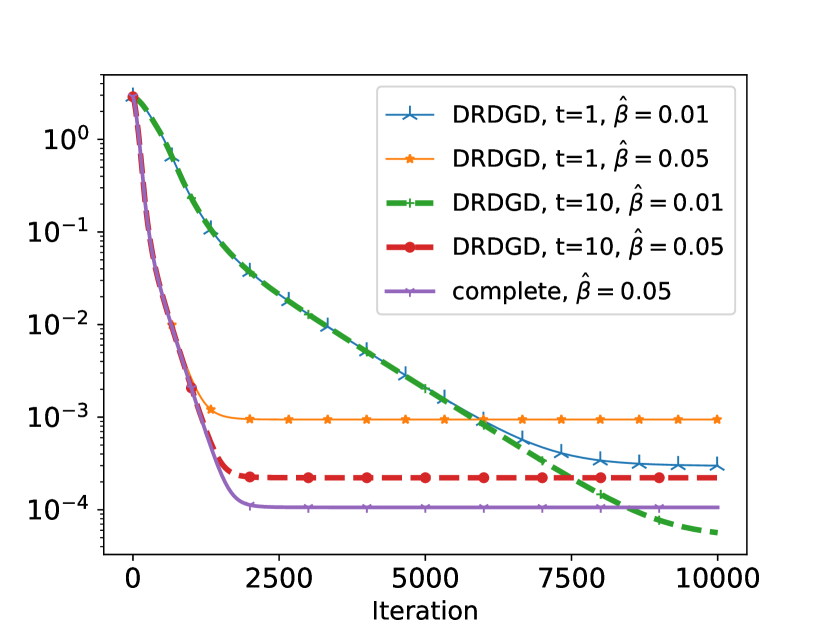
(b) DRDGD

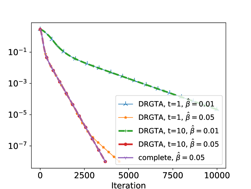
(c) DRGTA

Figure 1: Synthetic data, agents number $n=32,$ eigengap $\Delta=0.8$. y-axis: log-scale $d_{s}(\bar{x}_{k},x^{*})$.

In Figure 1, we show the results of DRSGD, DRDGD and DRGTA on the data with $n=32$ and $\Delta=0.8.$ The y-axis is the log-scale distance $d_{s}(\bar{x}_{k},x^{*}).$ The first four lines in each testing case are for the ring graph, and the last one is on a complete graph with equally weighted matrix, which aims to show the case of $t\rightarrow\infty$. In Figure 1(a), when fixing $\hat{\beta}$, it is shown that that smaller $\hat{\beta}$ produces higher accuracy, which indicates the Theorem 4.2. We also see DRSGD performs almost the same with different $t\in\{1,10,\infty\}$. For the two deterministic algorithms DRDGD and DRGTA, we see that DRDGD can use larger $\hat{\beta}$ if more communication rounds $t$ is used in Figure 1(b),(c). DRDGD cannot achieve exact convergence with the constant stepsize, while DRGTA successfully solves the problem using $t\in\{1,10,\infty\},\hat{\beta}=0.05.$

Next, we report the numerical results on different networks and data size.

Figure 2 shows the results on the same data set as that of Figure 1. However, the network is an Erdös-Rényi model $\mathsf{ER}(n,p)$, which means the probability of each edge is included in the graph with probability $p$. The Metropolis constant matrix is associated with the graph. Since the $\mathsf{ER}(32,0.3)$ is more well-connected than the ring graph, we see that the results for different $t\in\{1,10,\infty\}$ are almost the same except for DRDGD with $\hat{\beta}=0.05$. Moreover, the solutions accuracy and convergence rate of DRDGD and DRGTA are better than those shown in Figure 1.

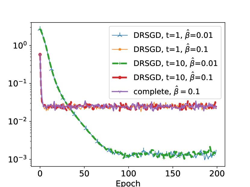
(a) DRSGD

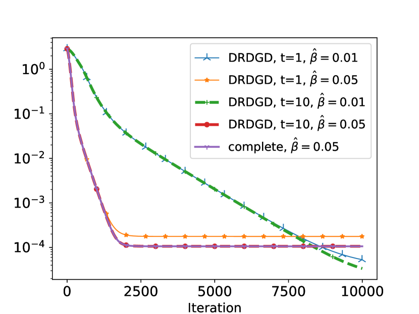
(b) DRDGD

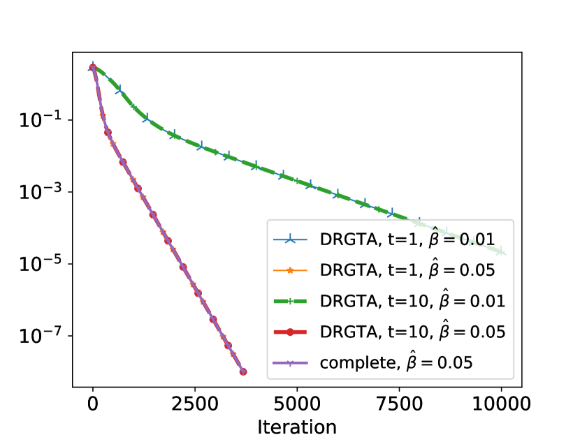
(c) DRGTA

Figure 2: Synthetic data, agents number $n=32,$ eigengap $\Delta=0.8$, Graph: $\mathsf{ER}(32,0.3).$ y-axis: log-scale $d_{s}(\bar{x}_{k},x^{*})$.

In Figure 3, we show the results when the initial point does not satisfy $\mathbf{x}_{0}\in\mathcal{N}$. Specifically, we randomly generate $x_{1,0},\ldots,x_{n,0}$ on $\mathcal{M},$ and the other settings are the same as Figure 1. Surprisingly, we find that the proposed algorithms still converge. As suggested by [26, 9], the consensus algorithm can achieve global consensus with random initialization when $r\leq\frac{2}{3}d-1$. The iteration in DRSGD and DRGTA is a perturbation of the consensus iteration. It will be interesting to study it further.

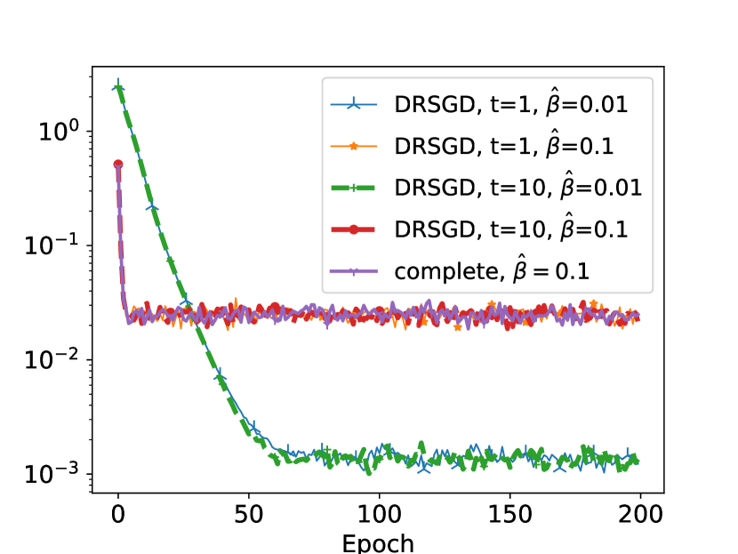
(a) DRSGD

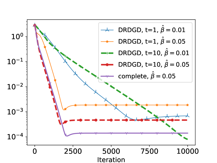
(b) DRDGD

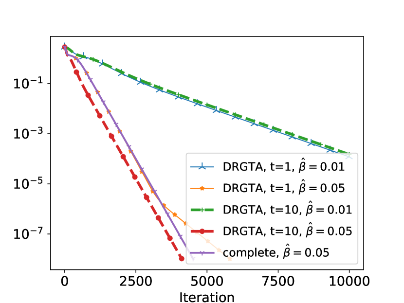
(c) DRGTA

Figure 3: Synthetic data, agents number $n=32,$ eigengap $\Delta=0.8$, Graph: Ring. y-axis: log-scale $d_{s}(\bar{x}_{k},x^{*})$.

6.2 Real-world data

We compare our algorithms with a recently proposed algorithm decentralized Sanger’s algorithm (DSA) [15], which is a Euclidean-type algorithm. To solve the eigenvector problem (6.1), DSA is shown to converge linearly to a neighborhood of the optimal solution. The computation of DSA iteration is cheaper than DRDGD since there is no retraction step. For simplicity, we fix $t=1$ and $r=5$ in this section.

We provide some numerical results on the MNIST dataset[21]. The graph is still the ring and $W$ is the Metropolis constant weight matrix. For MNIST, there are $60000$ samples and the dimension is given by $d=784.$ We normalize the data matrix by dividing $255$ such that the elements are in $[0,1].$ The data set is evenly partitioned into $n$ subsets. The stepsizes of DRDGD and DRGTA are set to $\beta=\frac{\hat{\beta}}{60000}.$

The results for MNIST data set with $n=20,40$ are shown in Figure 4. We see that the convergence rate of DSA and DRDGD are almost the same and DRGTA with $\hat{\beta}=0.1$ can achieve the most accurate solution. When $n$ becomes larger, the convergence rate of all algorithms is slower. Although the computation of DSA is cheaper than DRDGD, we find that when $\hat{\beta}=0.5,n=20,$ DSA does not converge, which is not shown in the Figure 4 (a). This is probably because DSA is not a feasible method and needs carefully tuned stepsize.

(a) MNIST, $n=20$, ring graph

(b) MNIST, $n=40$, ring graph

Figure 4: Numerical results of DRDGD, DRGTA, DSA on MNIST data set. y-axis: log-scale $d_{s}(\bar{x}_{k},x^{*})$.

Finally, we demonstrate the linear speedup of DRSGD for different $n$. The experiments are evaluated in a HPC cluster, where each computation node is associated with an Intel Xeon E5-2670 v2 CPU. The computation nodes are connected by FDR10 Infiniband. We use $10$ CPU cores each computation node in the HPC cluster. And we treat one CPU core as one network node in our problem. The codes are implemented in python with mpi4py.

We set the maximum epoch as $300$ in all experiments. The stepsize is set to $\beta=\frac{\sqrt{n}}{10000\sqrt{300}}\hat{\beta},$ where $\hat{\beta}$ is tuned for the best performance. The results in Figure 5 are $\log d_{s}(\bar{x}_{k},x^{*})$ v.s. epoch and $\log d_{s}(\bar{x}_{k},x^{*})$ v.s. CPU time, respectively. As we see in Figure 5(a), the solutions accuracy of $n=16,32,60$ are almost the same, while the CPU time in Figure 5(b) can be accelerated by nearly linear ratio.

(a) iteration

(b) time

Figure 5: Comparison results of different number of nodes on MNIST. Ring graph associated with Metropolis constant weight matrix, $t=1,$ $\beta=\frac{\sqrt{n}}{10000\sqrt{300}}\hat{\beta}.$ y-axis: log-scale $d_{s}(\bar{x}_{k},x^{*})$.

7 Conclusions

We discuss the decentralized optimization problem over Stiefel manifold and propose the two decentralized Riemannian gradient method and establish their convergence rate. Future topics could be cast into the following several folds: Firstly, for the eigenvector problem (6.1), it will be interesting to establish the linear convergence of DRGTA. Secondly, the analysis is based on the local convergence of Riemannian consensus, which results in multi-step consensus. It would be interesting to design algorithms based on Euclidean consensus.

Appendix A About the polar retraction

Given the polar decomposition of $x+\xi=QH,$ where $Q\in\mathbb{R}^{d\times r}$ is orthogonal and $H\in\mathbb{R}^{r\times r}$ is positive definite. The polar retraction is the polar factor

$$\mathcal{R}_{x}(\xi)=Q=(x+\xi)(I_{r}+\xi^{\top}\xi)^{-1/2},$$ (A.1)

which is also the orthogonal projection of $x+\xi$ onto $\mathrm{St}(d,r)$. The computation complexity is $\mathcal{O}(dr^{2}).$ [24, Append. E] showed that if $\|\xi\|_{\text{F}}\leq 1$ then $M=1$ for polar retraction. The boundedness of $\xi$ can be verified in our convergence analysis. Therefore, we have $M=1$ in this paper.

Appendix B More details on linear rate of consensus

The following results were provided in [9].

If there exists an integer $t\geq 0$ such that

$$\max_{i\in[n]}\|\sum_{j=1}^{n}(W_{ij}^{t}-1/n)(x_{j}-\bar{x})\|_{\text{F}}\leq\max_{i\in[n]}\sum_{j=1}^{n}|W_{ij}^{t}-1/n|\|\mathbf{x}-\bar{\mathbf{x}}\|_{\text{F},\infty}\leq\frac{1}{2}\|\mathbf{x}-\bar{\mathbf{x}}\|_{\text{F},\infty},$$ (B.1)

then it suffices to show the sequence $\{\mathbf{x}_{k}\}$ of DRCS satisfying $\mathbf{x}_{k}\in\mathcal{N}$ with $t\geq\lceil\log_{\sigma_{2}}(\frac{1}{2\sqrt{n}})\rceil$ steps of communication.

Denote the smallest eigenvalue of $W^{t}$ by $\lambda_{n}(W^{t}),$ the constant $L_{t}$ is given by

$$L_{t}=1-\lambda_{n}(W^{t}).$$ (B.2)

It is the Lipschitz constant of $\nabla\varphi^{t}(\mathbf{x})$. Since $L_{t}\in(0,2],$ if $\lambda_{n}(W^{t})$ is unknown, one can use $L_{t}=2.$ Define the second largest eigenvalue of $W^{t}$ by $\lambda_{2}(W^{t})$ and

$$\mu_{t}=1-\lambda_{2}(W^{t}).$$

The formal statement of Fact 3.1 is given as follows.

Fact B.1.

[9] Under Assumption 1, let the stepsize $\alpha$ satisfy $0<\alpha\leq\bar{\alpha}:=\min\{\nu\frac{\Phi}{L_{t}},1,\frac{1}{M}\}$ and $t\geq\lceil\log_{\sigma_{2}}(\frac{1}{2\sqrt{n}})\rceil$, where $\nu\in[0,1],$ $\Phi=2-\delta_{2}^{2}$ and $M$ is given in Lemma 2.3. The sequence $\{\mathbf{x}_{k}\}$ of (3.2) achieves consensus linearly if the initialization satisfies $\mathbf{x}_{0}\in\mathcal{N}$ defined by (3.6). That is, we have $\mathbf{x}_{k}\in\mathcal{N}$ for all $k\geq 0$ and

$$\begin{aligned} \|\mathbf{x}_{k+1}-\bar{\mathbf{x}}_{k+1}\|_{\text{F}}&\leq\|\mathbf{x}_{k}-\alpha\mathrm{grad}\varphi^{t}(\mathbf{x}_{k})-\bar{\mathbf{x}}_{k}\|_{\text{F}}\\ &\leq\sqrt{1-2(1-\nu)\alpha\gamma_{t}}\|\mathbf{x}_{k}-\bar{\mathbf{x}}_{k}\|_{\text{F}},\end{aligned}$$ (B.3)

where $\gamma_{t}=(1-4r\delta_{1}^{2})(1-\frac{\delta_{2}^{2}}{2})\mu_{t}\geq\frac{\mu_{t}}{2}\geq\frac{1-\sigma_{2}^{t}}{2}$.

If $\nu=1/2$, we have $\alpha\leq\bar{\alpha}:=\min\{\frac{\Phi}{2L_{t}},1,1/M\}$ and

$$\rho_{t}=\sqrt{1-\gamma_{t}\alpha}.$$

Recall that $M$ is the constant given in Lemma 2.3. We also have $M=\mathcal{O}(1)$ which is discussed in appendix A. If $\alpha=1$ is admissible, then the rate is $\rho_{t}=\sqrt{\frac{1+\sigma_{2}^{t}}{2}}$ which is worse that the Euclidean rate $\sigma_{2}^{t}.$ Moreover, it was shown in [9] in a smaller region, i.e., $\varphi^{t}(\mathbf{x})=\mathcal{O}(\sigma_{2}^{t})$ and $\|\mathbf{x}-\bar{\mathbf{x}}\|_{\text{F}}^{2}=\mathcal{O}(1),$ it follows asymptotically $\rho_{t}=\sigma_{2}^{t}$ with $\alpha=1$. For simplicity, we will only discuss the convergence of our proposed algorithms using (B.3) with $\nu=1/2$. Note that this may imply $\bar{\alpha}<1$, but we find that $\alpha=1$ always works for our proposed algorithms.

Appendix C Proofs for Section 2

Denote $\mathcal{P}_{N_{x}\mathcal{M}}$ as the orthogonal projection onto the normal space $N_{x}\mathcal{M}$. One can rewrite the projection $\mathcal{P}_{\mathrm{T}_{x}\mathcal{M}}(y-x),\forall y\in\mathrm{St}(d,r)$ [9] as follows

$$\quad\mathcal{P}_{\mathrm{T}_{x}\mathcal{M}}(y-x)=y-x-\mathcal{P}_{N_{x}\mathcal{M}}(y-x)$$ (P2)

$$=y-x+\frac{1}{2}x(x-y)^{\top}(x-y).$$

This implies that

$$\mathcal{P}_{\mathrm{T}_{x}\mathcal{M}}(y-x)=y-x+\mathcal{O}(\|y-x\|_{\text{F}}^{2}).$$

The relationship (P2) helps us to prove Lemma 2.4.

Proof of Lemma 2.4.

Firstly, since $\nabla f(x)$ is $L-$Lipschitz in Euclidean space, one has

$$\left|f(y)-\left[f(x)+\left\langle\nabla f(x),y-x\right\rangle\right]\right|\leq\frac{L}{2}\|y-x\|_{\text{F}}^{2}.$$ (C.1)

Since $\mathrm{grad}f(x)=\mathcal{P}_{\mathrm{T}_{x}\mathcal{M}}\nabla f(x)$, we have

$$\left\langle\mathrm{grad}f(x),y-x\right\rangle =\left\langle\nabla f(x),\mathcal{P}_{\mathrm{T}_{x}\mathcal{M}}(y-x)\right\rangle$$

$$\stackrel{{\scriptstyle\eqref{property of projection onto tangent}}}{{=}}\left\langle\nabla f(x),y-x\right\rangle+\left\langle\nabla f(x),\frac{1}{2}x(y-x)^{\top}(y-x)\right\rangle.$$

Using

$$\left\langle\nabla f(x),\frac{1}{2}x(y-x)^{\top}(y-x)\right\rangle\leq\|\nabla f(x)\|_{2}\cdot\|x\|_{2}\cdot\frac{1}{2}\|x-y\|_{\text{F}}^{2}\leq\frac{1}{2}\|\nabla f(x)\|_{2}\cdot\|x-y\|_{2}^{2}$$

implies

$$\left|\left\langle\mathrm{grad}f(x),y-x\right\rangle-\left\langle\nabla f(x),y-x\right\rangle\right|\leq\frac{1}{2}\max_{x\in\mathrm{St}(d,r)}\|\nabla f(x)\|_{2}\cdot\|y-x\|_{\text{F}}^{2},$$ (C.2)

where $\|\nabla f(x)\|_{2}$ represents the operator norm of $\nabla f(x)$. Since $\mathrm{St}(d,r)$ is a compact set and $\nabla f(x)$ is continuous, we denote $L_{n}=\max_{x\in\mathrm{St}(d,r)}\|\nabla f(x)\|_{2}$. Let $L_{g}=L_{n}+L$. Combining (C.1) with (C.2) yields

$$\left|f(y)-\left[f(x)+\left\langle\mathrm{grad}f(x),y-x\right\rangle\right]\right|\leq\frac{L_{g}}{2}\|y-x\|_{\text{F}}^{2}.$$ (C.3)

Secondly, using $\mathrm{grad}f(x)=\nabla f(x)-\mathcal{P}_{N_{x}\mathcal{M}}\nabla f(x)$ and $\mathrm{grad}f(y)=\nabla f(y)-\mathcal{P}_{N_{y}\mathcal{M}}\nabla f(y)$ implies

$$\quad\|\mathrm{grad}f(x)-\mathrm{grad}f(y)\|_{\text{F}}$$

$$\leq\|\nabla f(x)-\nabla f(y)\|_{\text{F}}+\|\mathcal{P}_{N_{x}\mathcal{M}}\nabla f(y)-\mathcal{P}_{N_{y}\mathcal{M}}\nabla f(y)\|_{\text{F}}$$

$$=\|\nabla f(x)-\nabla f(y)\|_{\text{F}}+\frac{1}{2}\|x(x^{\top}\nabla f(y)+\nabla f(y)^{\top}x)-y(y^{\top}\nabla f(y)+\nabla f(y)^{\top}y)\|_{\text{F}}$$

$$\leq\|\nabla f(x)-\nabla f(y)\|_{\text{F}}+2L_{n}\|x-y\|_{\text{F}}$$ (C.4)

$$\leq(L+2L_{n})\|x-y\|_{\text{F}}.$$

In (C.4) we used

$$\quad\|x(x^{\top}\nabla f(y)+\nabla f(y)^{\top}x)-y(y^{\top}\nabla f(y)+\nabla f(y)^{\top}y)\|_{\text{F}}$$

$$\leq\|x((x-y)^{\top}\nabla f(y)+\nabla f(y)^{\top}(x-y))\|_{\text{F}}+\|(x-y)(y^{\top}\nabla f(y)+\nabla f(y)^{\top}y)\|_{\text{F}}$$

$$\leq 4L_{n}\|x-y\|_{\text{F}}.$$

The proof is completed. ∎

C.1 Comparison on different Lipschitz-type inequalities

Using Taylor’s Theorem[1, Lemma 7.4.7], $L_{g}^{\prime}$ corresponds to the leading eigenvalue of Riemannian Hessian. According to [2], it follows for any $\eta\in\mathrm{T}_{x}\mathcal{M}$ that

$$\mathrm{Hess}f(x)[\eta] =\mathcal{P}_{T_{x\mathcal{M}}}\left(D\mathrm{grad}h(x)[\eta]\right)$$ (C.5)

$$=\mathcal{P}_{T_{x}\mathcal{M}}\nabla^{2}f(x)\eta-\eta x^{\top}\mathcal{P}_{N_{x}}\nabla f(x)-x\frac{1}{2}\left(\eta^{\top}\mathcal{P}_{N_{x}}\nabla f(x_{i})+(\mathcal{P}_{N_{x}}\nabla f(x))^{\top}\eta\right),$$

where $\mathcal{P}_{N_{x}}$ is the orthogonal projection onto the normal space $N_{x}\mathcal{M}$. Since $x\frac{1}{2}\left(\eta^{\top}\mathcal{P}_{N_{x}}\nabla f(x_{i})+(\mathcal{P}_{N_{x}}\nabla f(x))^{\top}\eta\right)\in N_{x}\mathcal{M}$, we have

$$\left\langle\eta,\mathrm{Hess}f(x)[\eta]\right\rangle=\left\langle\eta,\nabla^{2}f(x)\eta\right\rangle-\left\langle\eta,\eta x^{\top}\mathcal{P}_{N_{x}}\nabla f(x)\right\rangle=\left\langle\eta,\nabla^{2}f(x)\eta\right\rangle-\left\langle\eta,\eta\frac{1}{2}(x^{\top}\nabla f(x)+\nabla f(x)^{\top}x)\right\rangle,$$ (C.6)

where we use $\mathcal{P}_{T_{x}\mathcal{M}}\nabla^{2}f(x)\eta=\nabla^{2}f(x)\eta-\mathcal{P}_{N_{x}}\nabla^{2}f(x)\eta$. Therefore, we get

$$L_{g}^{\prime}\leq\lambda_{\max}(\nabla^{2}f(x))+\max_{x\in\mathrm{St}(d,r)}\|\nabla f(x)\|_{2}=L+L_{n}.$$ (C.7)

The restricted inequality proposed in [7] is related to the pull back function $g(\xi):=f(\mathcal{R}_{x}(\xi))$, whose Lipschitz constant $\tilde{L}_{g}$ relies on the retraction. Specifically, $\tilde{L}_{g}=M_{0}^{2}L+2ML_{n}$, where $M_{0}$ is a constant related to the retraction, $M$ and $L_{n}$ are the same constants in Lemma 2.3.

C.2 Technical lemmas

Lemma C.1.

[9] For any $\mathbf{x}\in\mathrm{St}(d,r)^{n}$, let $\hat{x}=\frac{1}{n}\sum_{i=1}^{n}x_{i}$ be the Euclidean mean and denote $\hat{\mathbf{x}}=\mathbf{1}_{n}\otimes\hat{x}$. Similarly, let $\bar{\mathbf{x}}=\mathbf{1}_{n}\otimes\bar{x}$, where $\bar{x}$ is the IAM defined in (IAM). Moreover, if $\|\mathbf{x}-\bar{\mathbf{x}}\|_{\text{F}}^{2}\leq n/2$, one has

$$\|\bar{x}-\hat{x}\|_{\text{F}}\leq\frac{2\sqrt{r}\|\mathbf{x}-\bar{\mathbf{x}}\|_{\text{F}}^{2}}{n}.$$ (P1)

The following lemma will be useful to bound the Euclidean distance between two average points $\bar{x}_{k}$ and $\bar{x}_{k+1}$.

Lemma C.2.

[9] Suppose $\mathbf{x},\mathbf{y}\in\mathcal{N}_{1}$, where $\mathcal{N}_{1}$ is defined in (3.4). Then we have

$$\|\bar{x}-\bar{y}\|_{\text{F}}\leq\frac{1}{1-2\delta_{1}^{2}}\|\hat{x}-\hat{y}\|_{\text{F}},$$

where $\bar{x}$ and $\bar{y}$ are the IAM of $x_{1},\ldots,x_{n}$ and $y_{1},\ldots,y_{n}$, respectively.

We also need the following bounds for $\mathrm{grad}\varphi^{t}(\mathbf{x})$.

Lemma C.3.

[9] For any $\mathbf{x}\in\mathrm{St}(d,r)^{n}$, it follows that

$$\|\sum_{i=1}^{n}\mathrm{grad}\varphi^{t}(x_{i})\|_{\text{F}}\leq L_{t}\|\mathbf{x}-\bar{\mathbf{x}}\|_{\text{F}}^{2}$$ (C.8)

and

$$\|\mathrm{grad}\varphi^{t}(\mathbf{x})\|_{\text{F}}\leq L_{t}\|\mathbf{x}-\bar{\mathbf{x}}\|_{\text{F}},$$ (C.9)

where $L_{t}$ is the constant given in (B.2). Moreover, suppose $\mathbf{x}\in\mathcal{N}_{2}$, where $\mathcal{N}_{2}$ is defined by (3.5). We then have

$$\max_{i\in[n]}\|\mathrm{grad}\varphi^{t}_{i}(\mathbf{x})\|_{\text{F}}\leq 2\delta_{2}.$$ (C.10)

Applying Lemma C.2 to the update rule of our algorithms gives the following lemma.

Lemma C.4.

If $\mathbf{x}_{k}\in\mathcal{N},\mathbf{x}_{k+1}\in\mathcal{N}_{1}$ and $x_{i,k+1}=\mathcal{R}_{x_{i,k}}(-\alpha\mathrm{grad}\varphi_{i}^{t}(\mathbf{x}_{k})+\beta u_{i,k})$, where $u_{i,k}\in\mathrm{T}_{x_{i,k}}\mathcal{M}$, $0\leq\alpha\leq\frac{1}{M}$, $0\leq\beta$. Let $\mathbf{u}_{k}^{\top}=(u_{1,k}^{\top}\ \ldots\ u_{n,k}^{\top})$ and $\hat{u}_{k}=\frac{1}{n}\sum_{i=1}^{n}u_{i,k}$. It follows that

$$\|\bar{x}_{k}-\bar{x}_{k+1}\|_{\text{F}}\leq\frac{1}{1-2\delta_{1}^{2}}\left(\frac{2L_{t}^{2}\alpha+L_{t}\alpha}{n}\|\mathbf{x}_{k}-\bar{\mathbf{x}}_{k}\|_{\text{F}}^{2}+{\beta}\|\hat{u}_{k}\|_{\text{F}}+\frac{2M\beta^{2}}{n}\|\mathbf{u}_{k}\|_{\text{F}}^{2}\right).$$

Proof.

From Lemma 2.3 and Lemma C.3, we have

$$\quad\|\hat{x}_{k}-\hat{x}_{k+1}\|_{\text{F}}$$

$$\leq\|\hat{x}_{k}+\frac{1}{n}\sum_{i=1}^{n}(-\alpha\mathrm{grad}\varphi_{i}^{t}(\mathbf{x}_{k})+\beta u_{i,k})-\hat{x}_{k+1}\|_{\text{F}}+\|\frac{1}{n}\sum_{i=1}^{n}(-\alpha\mathrm{grad}\varphi_{i}^{t}(\mathbf{x}_{k})+\beta u_{i,k})\|_{\text{F}}$$

$$\stackrel{{\scriptstyle\eqref{ineq:ret_second-order}}}{{\leq}}\frac{M}{n}\sum_{i=1}^{n}\|\alpha\mathrm{grad}\varphi_{i}^{t}(\mathbf{x}_{k})+\beta u_{i,k}\|_{\text{F}}^{2}+\alpha\|\frac{1}{n}\sum_{i=1}^{n}\mathrm{grad}\varphi_{i}^{t}(\mathbf{x}_{k})\|_{\text{F}}+\beta\|\hat{u}_{k}\|_{\text{F}}$$

$$\leq\frac{2M\alpha^{2}}{n}\|\mathrm{grad}\varphi^{t}(\mathbf{x}_{k})\|_{\text{F}}^{2}+\frac{2M\beta^{2}}{n}\|\mathbf{u}_{k}\|_{\text{F}}^{2}+\alpha\|\frac{1}{n}\sum_{i=1}^{n}\mathrm{grad}\varphi_{i}^{t}(\mathbf{x}_{k})\|_{\text{F}}+\beta\|\hat{u}_{k}\|_{\text{F}}$$

$$\stackrel{{\scriptstyle\eqref{ineq:bound-of-gradh}\eqref{ineq:bound-of-sum-gradh}}}{{\leq}}\frac{2L_{t}^{2}M\alpha^{2}+L_{t}\alpha}{n}\|\mathbf{x}_{k}-\bar{\mathbf{x}}_{k}\|_{\text{F}}^{2}+\frac{2M\beta^{2}}{n}\|\mathbf{u}_{k}\|_{\text{F}}^{2}+\beta\|\hat{u}_{k}\|_{\text{F}}.$$

Therefore, it follows from Lemma C.2 that

$$\|\bar{x}_{k}-\bar{x}_{k+1}\|_{\text{F}}\leq\frac{1}{1-2\delta_{1}^{2}}\|\hat{x}_{k}-\hat{x}_{k+1}\|_{\text{F}}\leq\frac{1}{1-2\delta_{1}^{2}}\left(\frac{2L_{t}^{2}\alpha+L_{t}\alpha}{n}\|\mathbf{x}_{k}-\bar{\mathbf{x}}_{k}\|_{\text{F}}^{2}+{\beta}\|\hat{u}_{k}\|_{\text{F}}+\frac{2M\beta^{2}}{n}\|\mathbf{u}_{k}\|_{\text{F}}^{2}\right),$$

where we use the fact that $\alpha\leq\frac{1}{M}$. ∎

Appendix D Proofs for Section 4

We use the notations

$$\mathbf{v}_{k}=[v_{1,k}^{\top}\ \ldots\ v_{n,k}^{\top}]^{\top},\quad\hat{v}_{k}=\frac{1}{n}\sum_{i=1}^{n}v_{i,k},$$

$$g_{i,k}=\mathrm{grad}f_{i}(x_{i,k})\quad\textit{and}\quad\hat{g}_{k}=\frac{1}{n}\sum_{i=1}^{n}g_{i,k}.$$

The following lemma is useful to show $\mathbf{x}_{k}\in\mathcal{N}$ for all $k.$

Lemma D.1.

[9, Lemma 11] Given any $\mathbf{x}\in\mathcal{N}_{2}$, where $\mathcal{N}_{2}$ is defined in (3.5), if $t\geq\lceil\log_{\sigma_{2}}(\frac{1}{2\sqrt{n}})\rceil$, we have

$$\max_{i\in[n]}\|\sum_{j=1}^{n}(W^{t}_{ij}-1/n)x_{j}\|_{\text{F}}\leq\frac{\delta_{2}}{2}.$$ (D.1)

Lemma D.2.

Under the same conditions of Fact B.1, if $\mathbf{x}_{k}\in\mathcal{N}$ and

$$x_{i,k+1}=\mathcal{R}_{x_{i,k}}(-\alpha\mathrm{grad}\varphi_{i}^{t}(\mathbf{x}_{k})+\beta v_{i,k}),\quad\forall i\in[n],$$

where $v_{i,k}\in\mathrm{T}_{x_{i,k}}\mathcal{M}$, the following holds

$$\|\mathbf{x}_{k+1}-\bar{\mathbf{x}}_{k+1}\|_{\text{F}}\leq\rho_{t}\|\mathbf{x}_{k}-\bar{\mathbf{x}}_{k}\|_{\text{F}}+\beta_{k}\|\mathbf{v}_{k}\|_{\text{F}}.$$

Proof.

By the definition of IAM, we have

$$\|\mathbf{x}_{k+1}-\bar{\mathbf{x}}_{k+1}\|_{\text{F}}^{2}\leq\|\mathbf{x}_{k+1}-\bar{\mathbf{x}}_{k}\|_{\text{F}}^{2}$$ (D.2)

$$= \sum_{i=1}^{n}\|\mathcal{R}_{x_{i,k}}\left(-\alpha\mathrm{grad}\varphi_{i}^{t}(\mathbf{x}_{k})-\beta_{k}v_{i,k}\right)-\bar{x}_{k}\|_{\text{F}}^{2}$$

$$\stackrel{{\scriptstyle\eqref{ineq:ret_nonexpansive}}}{{\leq}} \sum_{i=1}^{n}\|x_{i,k}-\alpha\mathrm{grad}\varphi_{i}^{t}(\mathbf{x}_{k})-\beta_{k}v_{i,k}-\bar{x}_{k}\|_{\text{F}}^{2}.$$

Let $\mathbf{v}_{k}=[v_{1,k}^{\top}\ \ldots\ v_{n,k}^{\top}]^{\top}$. Then, we get

$$\|\mathbf{x}_{k+1}-\bar{\mathbf{x}}_{k+1}\|_{\text{F}} \leq\|\mathbf{x}_{k}-\alpha\mathrm{grad}\varphi^{t}(\mathbf{x}_{k})-\beta_{k}\mathbf{v}_{k}-\bar{\mathbf{x}}_{k}\|_{\text{F}}$$ (D.3)

$$\leq\|\mathbf{x}_{k}-\alpha\mathrm{grad}\varphi^{t}(\mathbf{x}_{k})-\bar{\mathbf{x}}_{k}\|_{\text{F}}+\beta_{k}\|\mathbf{v}_{k}\|_{\text{F}}.$$

By combining inequality (B.3) of Fact B.1, we get

$$\|\mathbf{x}_{k+1}-\bar{\mathbf{x}}_{k+1}\|_{\text{F}} \leq\rho_{t}\|\mathbf{x}_{k}-\bar{\mathbf{x}}_{k}\|_{\text{F}}+\beta_{k}\|\mathbf{v}_{k}\|_{\text{F}}.$$ (D.4)

The proof is completed.

∎

Proof of Lemma 4.1 .

We prove that $\mathbf{x}_{k}\in\mathcal{N}$ for all $k\geq 0$ by induction. Suppose $\mathbf{x}_{k}\in\mathcal{N}$, let us show $\mathbf{x}_{k+1}\in\mathcal{N}.$ Note $\|\mathbf{v}_{k}\|_{\text{F}}\leq\sqrt{n}D.$ Using Lemma D.2 yields

$$\|\mathbf{x}_{k+1}-\bar{\mathbf{x}}_{k+1}\|_{\text{F}} \leq\rho_{t}\|\mathbf{x}_{k}-\bar{\mathbf{x}}_{k}\|_{\text{F}}+\beta_{k}\sqrt{n}D$$ (D.5)

$$\leq\rho_{t}\sqrt{n}\delta_{1}+\beta_{k}\sqrt{n}D$$

$$\leq\sqrt{n}\delta_{1},$$

where the last inequality follows from $\beta_{k}\leq\frac{1-\rho_{t}}{D}\delta_{1}$. Hence $\mathbf{x}_{k+1}\in\mathcal{N}_{1}$. Secondly, let us verify $\mathbf{x}_{k+1}\in\mathcal{N}_{2}$. It follows from $\beta_{k}\leq\frac{\alpha\delta_{1}}{5D}\leq\frac{\alpha}{2D}$ and $\alpha\leq 1$ that

$$\|\mathbf{x}_{k+1}-{\mathbf{x}}_{k}\|_{\text{F},\infty}\stackrel{{\scriptstyle\eqref{ineq:ret_nonexpansive}}}{{\leq}}\max_{i\in[n]}\|\alpha\mathrm{grad}\varphi^{t}(x_{k,i})\|_{\text{F}}+\beta_{k}D\stackrel{{\scriptstyle\eqref{ineq:bound-of-gradh-i}}}{{\leq}}2\alpha\delta_{2}+\frac{\alpha}{2}\leq 1-\delta_{1}^{2}.$$

Using Lemma C.4 yields

$$\|\bar{x}_{k}-\bar{x}_{k+1}\|_{\text{F}} \leq\frac{1}{1-2\delta_{1}^{2}}\left(\frac{2L_{t}^{2}\alpha+L_{t}\alpha}{n}\|\mathbf{x}_{k}-\bar{\mathbf{x}}_{k}\|_{\text{F}}^{2}+{\beta}\|\hat{v}_{k}\|_{\text{F}}+\frac{2M\beta_{k}^{2}}{n}\|\mathbf{v}_{k}\|_{\text{F}}^{2}\right)$$

$$\leq\frac{1}{1-2\delta_{1}^{2}}\left[(2L_{t}^{2}\alpha+L_{t}\alpha)\delta_{1}^{2}+\beta_{k}D+2M\beta_{k}^{2}D^{2}\right].$$

Furthermore, since $L_{t}\leq 2$, $\beta_{k}\leq\frac{\alpha\delta_{1}}{5D}$, $\alpha\leq 1/M$, we get

$$\|\bar{x}_{k}-\bar{x}_{k+1}\|_{\text{F}}\leq\frac{1}{1-2\delta_{1}^{2}}\left(\frac{252}{25}\alpha\delta_{1}^{2}+\frac{\alpha\delta_{1}}{5}\right)\leq\frac{1}{1-2\delta_{1}^{2}}\left(\frac{252}{625r}\alpha\delta_{2}^{2}+\frac{1}{25\sqrt{r}}\alpha\delta_{2}\right),$$ (D.6)

where the last inequality follows from $\delta_{1}\leq\frac{1}{5\sqrt{r}}\delta_{2}$. Then, one has

$$\|x_{i,k+1}-\bar{x}_{k+1}\|_{\text{F}}$$

$$\leq \|x_{i,k+1}-\bar{x}_{k}\|_{\text{F}}+\|\bar{x}_{k}-\bar{x}_{k+1}\|_{\text{F}}$$

$$\stackrel{{\scriptstyle\eqref{ineq:ret_nonexpansive}}}{{\leq}} \|x_{i,k}-\alpha\mathrm{grad}\varphi_{i}^{t}(\mathbf{x}_{k})-\beta_{k}v_{i,k}-\bar{x}_{k}\|_{\text{F}}+\|\bar{x}_{k}-\bar{x}_{k+1}\|_{\text{F}}$$

$$\leq \|x_{i,k}-\alpha\mathrm{grad}\varphi_{i}^{t}(\mathbf{x}_{k})-\bar{x}_{k}\|_{\text{F}}+\frac{1}{5}\alpha\delta_{1}+\|\bar{x}_{k}-\bar{x}_{k+1}\|_{\text{F}}.$$ (D.7)

Now, we proceed by using the same lines in the proof of [9, Lemma 13] as follows

$$\mathrm{grad}\varphi^{t}_{i}(\mathbf{x})=x_{i}-\sum_{j=1}^{n}W_{ij}x_{j}-\frac{1}{2}x_{i}\sum_{j=1}^{n}W_{ij}^{t}(x_{i}-x_{j})^{\top}(x_{i}-x_{j}),$$ (D.8)

and

$$\|x_{i,k}-\alpha\mathrm{grad}\varphi_{i}^{t}(\mathbf{x}_{k})-\bar{x}_{k}\|_{\text{F}}$$

$$\stackrel{{\scriptstyle\eqref{rewrite}}}{{=}} \|(1-\alpha)(x_{i,k}-\bar{x}_{k})+\alpha(\hat{x}_{k}-\bar{x}_{k})+\alpha\sum_{j=1}^{n}{W}_{ij}^{t}(x_{j,k}-\hat{x}_{k})+\frac{\alpha}{2}x_{i,k}\sum_{j=1}^{n}W_{ij}^{t}(x_{i,k}-x_{j,k})^{\top}(x_{i,k}-x_{j,k})\|_{\text{F}}$$

$$\leq (1-\alpha)\delta_{2}+\alpha\|\hat{x}_{k}-\bar{x}_{k}\|_{\text{F}}+\alpha\|\sum_{j=1}^{n}({W}_{ij}^{t}-\frac{1}{n})x_{j,k}\|_{\text{F}}+\frac{1}{2}\|{\alpha}\sum_{j=1}^{n}W_{ij}^{t}(x_{i,k}-x_{j,k})^{\top}(x_{i,k}-x_{j,k})\|_{\text{F}}$$ (D.9)

$$\leq (1-\alpha)\delta_{2}+2\alpha\delta_{1,t}^{2}\sqrt{r}+\alpha\|\sum_{j=1}^{n}({W}_{ij}^{t}-\frac{1}{n})x_{j,k}\|_{\text{F}}+2{\alpha}\delta_{2}^{2}$$ (D.10)

$${\leq} (1-\frac{\alpha}{2})\delta_{2}+2\alpha\delta_{1}^{2}\sqrt{r}+2{\alpha}\delta_{2}^{2},$$ (D.11)

where (D.9) follows from $\alpha\in[0,1]$, (D.10) holds by Lemma C.1 and (D.11) follows from Lemma D.1. Combining this with (D.7) implies

$$\|x_{i,k+1}-\bar{x}_{k+1}\|_{\text{F}}$$

$$\leq (1-\frac{\alpha}{2})\delta_{2}+2\alpha\delta_{1}^{2}\sqrt{r}+2{\alpha}\delta_{2}^{2}+\frac{1}{5}\alpha\delta_{1}+\|\bar{x}_{k}-\bar{x}_{k+1}\|_{\text{F}}$$

$$\stackrel{{\scriptstyle\eqref{ineq:de0}}}{{\leq}} (1-\frac{\alpha}{2})\delta_{2}+2\alpha\delta_{1}^{2}\sqrt{r}+2{\alpha}\delta_{2}^{2}+\frac{1}{5}\alpha\delta_{1}+\frac{1}{1-2\delta_{1}^{2}}\left(\frac{252}{625r}\alpha\delta_{2}^{2}+\frac{1}{25\sqrt{r}}\alpha\delta_{2}\right).$$ (D.12)

Therefore, substituting the conditions (3.6) on $\delta_{1},\delta_{2}$ into (D.12) yields

$$\|x_{i,k+1}-\bar{x}_{k+1}\|_{\text{F}}\leq\delta_{2}.$$

The proof of the first statement is completed. Finally, it follows from (D.5) that

$$\|\mathbf{x}_{k+1}-\bar{\mathbf{x}}_{k+1}\|_{\text{F}} \leq\rho_{t}\|\mathbf{x}_{k}-\bar{\mathbf{x}}_{k}\|_{\text{F}}+\beta_{k}\sqrt{n}D$$ (D.13)

$$\leq\rho_{t}^{k+1}\|\mathbf{x}_{0}-\bar{\mathbf{x}}_{0}\|_{\text{F}}+\sqrt{n}D\sum_{l=0}^{k}\rho_{t}^{k-l}\beta_{l}.$$

∎

An immediate result of Lemma 4.1 is that the rate of consensus $\|\mathbf{x}_{k}-\bar{\mathbf{x}}_{k}\|_{\text{F}}^{2}=\mathcal{O}(\beta_{k}^{2})$ if $\beta_{k}=\mathcal{O}(\frac{1}{k^{p}})$. The proof is similar as [25, Proposition 8], we provide it for completeness.

Lemma D.3.

Under Assumptions 2, 1, 3 and 4, for Algorithm 1, if $\mathbf{x}_{0}\in\mathcal{N}$, $0<\alpha\leq\min\{\frac{\Phi}{2L_{t}},1,\frac{1}{M}\}$, $t\geq\lceil\log_{\sigma_{2}}(\frac{1}{2\sqrt{n}})\rceil$ and

$$\beta_{k}=\min\{\frac{\alpha\delta_{1}}{5D}\cdot\frac{1}{(k+1)^{p}},\frac{1-\rho_{t}}{D}\delta_{1}\},\quad p\in(0,1],$$ (D.14)

then there exists a constant $C>0$ such that $\frac{1}{n}\|\mathbf{x}_{k}-\bar{\mathbf{x}}_{k}\|_{\text{F}}^{2}\leq CD^{2}\beta_{k}^{2}$ for any $k\geq 0$, where $C$ is independent of $D$ and $n$.

Proof of Lemma D.3.

The proof relies on Lemma 4.1. Let $a_{k}:=\frac{\|\mathbf{x}_{k}-\bar{\mathbf{x}}_{k}\|_{\text{F}}}{\sqrt{n}\beta_{k}}$.

It follows from (D.13) that

$$a_{k+1} \leq\rho_{t}a_{k}+D\cdot\frac{\beta_{k}}{\beta_{k+1}}\leq\rho_{t}^{k+1-K}a_{K}+D\sum_{l=K}^{k}\rho_{t}^{k-l}\frac{\beta_{l}}{\beta_{l+1}}.$$ (D.15)

Recall that $\beta_{k}=\mathcal{O}(1/D)$ and $\frac{1}{n}\|\mathbf{x}_{0}-\bar{\mathbf{x}}_{0}\|_{\text{F}}^{2}\leq\delta_{1}^{2}$, it follows that $a_{0}\leq\delta_{1}/\beta_{0}=\mathcal{O}(D)$. Since $\lim_{k\rightarrow\infty}\frac{\beta_{k+1}}{\beta_{k}}=1$, there exists sufficiently large $K$ such that

$$\frac{\beta_{k}}{\beta_{k+1}}\leq 2,\quad\forall k\geq K.$$

For $0\leq k\leq K$, there exists some $C^{\prime}>0$ such that

$$a_{k}^{2}\leq C^{\prime}D^{2},$$

where $C^{\prime}$ is independent of $D$ and $n$. For $k\geq K$, using (D.15) gives $a_{k}^{2}\leq CD^{2}$, where $C=2C^{\prime}+\frac{8}{(1-\rho_{t})^{2}}$. Hence, we get $\|\mathbf{x}_{k}-\bar{\mathbf{x}}_{k}\|_{\text{F}}^{2}/n\leq CD^{2}\beta_{k}^{2}$ for all $k\geq 0$, where $C=\mathcal{O}(\frac{1}{(1-\rho_{t})^{2}})$. ∎

Lemma D.4.

Under Assumptions 2, 1, 3 and 4, suppose $\mathbf{x}_{k}\in\mathcal{N}$, $t\geq\lceil\log_{\sigma_{2}}(\frac{1}{2\sqrt{n}})\rceil$, $0<\alpha\leq\min\{\frac{\Phi}{2L_{t}},1,\frac{1}{M}\}$. If $x_{i,k+1}=\mathcal{R}_{x_{i,k}}(-\alpha\mathrm{grad}\varphi^{t}(x_{i,k})-\beta_{k}v_{i,k})$, $0<\beta_{k}\leq\min\{\frac{1}{5L_{g}},\frac{\alpha\delta_{1}}{5D}\}$ and $\beta_{k}\geq\beta_{k+1}$, where $v_{i,k}$ satisfies Assumption 3 and $L_{g}$ is given in Lemma 2.4. It follows that

$$\mathbb{E}_{k}f(\bar{x}_{k+1})\leq f(\bar{x}_{k})-\frac{\beta_{k}}{4}\|\hat{g}_{k}\|_{\text{F}}^{2}-\frac{\beta_{k}}{4}\|\mathrm{grad}f(\bar{x}_{k})\|_{\text{F}}^{2}$$ (D.16)

$$\quad+\frac{3L_{g}\Xi^{2}}{2n}\beta_{k}^{2}+(\frac{CD^{2}L_{G}^{2}}{2}+\mathcal{T}_{1}D^{4})\beta_{k}^{3}+\mathcal{T}_{2}L_{g}D^{4}\beta_{k}^{4},$$

where $L_{G}$ is given in Lemma 2.4, $C$ is given in Lemma D.3, $\mathcal{T}_{1}=2(4\sqrt{r}+6\alpha)^{2}C^{2}+8M^{2}$ and $\mathcal{T}_{2}=201\alpha^{2}C^{2}+9M^{2}.$

Note the variance term is in the order of $\mathcal{O}(\frac{\Xi^{2}}{n}\beta_{k}^{2})$, since the gradient batch size is $n$.

Proof of Lemma D.4.

Denote the conditional expectation $\mathbb{E}_{i,k}v_{i,k}:=\mathbb{E}[v_{i,k}|x_{i,k}]$ and $\mathbb{E}_{k}:=\mathbb{E}[\cdot|\mathbf{x}_{k}]$. By invoking Lemma 2.4, we have

$$\quad\mathbb{E}_{k}f(\bar{x}_{k+1})\leq f(\bar{x}_{k})+\left\langle\mathrm{grad}f(\bar{x}_{k}),\mathbb{E}_{k}\bar{x}_{k+1}-\bar{x}_{k}\right\rangle+\frac{L_{g}}{2}\mathbb{E}_{k}\|\bar{x}_{k+1}-\bar{x}_{k}\|_{\text{F}}^{2}$$ (D.17)

$$=f(\bar{x}_{k})-\left\langle\mathrm{grad}f(\bar{x}_{k}),\beta_{k}\hat{g}_{k}\right\rangle+\left\langle\mathrm{grad}f(\bar{x}_{k}),\mathbb{E}_{k}[\bar{x}_{k+1}-\bar{x}_{k}+\beta_{k}\hat{v}_{k}]\right\rangle+\frac{L_{g}}{2}\mathbb{E}_{k}\|\bar{x}_{k+1}-\bar{x}_{k}\|_{\text{F}}^{2}$$

$$=f(\bar{x}_{k})-\frac{\beta_{k}}{2}\|\mathrm{grad}f(\bar{x}_{k})\|_{\text{F}}^{2}-\frac{\beta_{k}}{2}\|\hat{g}_{k}\|_{\text{F}}^{2}+\frac{\beta_{k}}{2}\|\mathrm{grad}f(\bar{x}_{k})-\hat{g}_{k}\|_{\text{F}}^{2}$$

$$\quad+\left\langle\mathrm{grad}f(\bar{x}_{k}),\mathbb{E}_{k}\bar{x}_{k+1}-\bar{x}_{k}+\beta_{k}\hat{g}_{k}\right\rangle+\frac{L_{g}}{2}\mathbb{E}_{k}\|\bar{x}_{k+1}-\bar{x}_{k}\|_{\text{F}}^{2},$$

where $\hat{v}_{k}=\frac{1}{n}\sum_{i=1}^{n}v_{i,k}$ and we use $\mathbb{E}_{k}\hat{v}_{k}=\hat{g}_{k}$ in the first equation.

Note that for $\beta_{k}>0$, we have

$$\quad\left\langle\mathrm{grad}f(\bar{x}_{k}),\mathbb{E}_{k}\bar{x}_{k+1}-\bar{x}_{k}+\beta_{k}\hat{g}_{k}\right\rangle\leq\frac{\beta_{k}}{4}\|\mathrm{grad}f(\bar{x}_{k})\|_{\text{F}}^{2}+\frac{1}{\beta_{k}}\|\mathbb{E}_{k}\bar{x}_{k+1}-\bar{x}_{k}+\beta_{k}\hat{g}_{k}\|_{\text{F}}^{2}.$$

Plugging this into (D.17) yields

$$\quad\mathbb{E}_{k}f(\bar{x}_{k+1})$$ (D.18)

$$\leq f(\bar{x}_{k})-\frac{\beta_{k}}{2}\|\hat{g}_{k}\|_{\text{F}}^{2}-\frac{\beta_{k}}{4}\|\mathrm{grad}f(\bar{x}_{k})\|_{\text{F}}^{2}+\frac{\beta_{k}}{2}\underbrace{\|\mathrm{grad}f(\bar{x}_{k})-\hat{g}_{k}\|_{\text{F}}^{2}}_{:=a_{1}}+\frac{1}{\beta_{k}}\underbrace{\|\mathbb{E}_{k}[\bar{x}_{k+1}-\bar{x}_{k}+\beta_{k}\hat{v}_{k}]\|_{\text{F}}^{2}}_{:=a_{2}}$$

$$\quad+\frac{L_{g}}{2}\underbrace{\mathbb{E}_{k}\|\bar{x}_{k+1}-\bar{x}_{k}\|_{\text{F}}^{2}}_{:=a_{3}}.$$

Using Lemma 2.4 implies

$$a_{1}\leq\frac{1}{n}\sum_{i=1}^{n}\|\mathrm{grad}f(x_{i,k})-\mathrm{grad}f(\bar{x}_{k})\|_{\text{F}}^{2}\stackrel{{\scriptstyle\eqref{ineq:lips_riemanniangrad}}}{{\leq}}\frac{L_{G}^{2}}{n}\|\mathbf{x}_{k}-\bar{\mathbf{x}}_{k}\|_{\text{F}}^{2}.$$

Secondly, we use the following inequality to derive the upper bound of $a_{2}$. From Lemma 4.1, we have $\mathbf{x}_{k+1}\in\mathcal{N}$. One has

$$\quad\|\bar{x}_{k+1}-\bar{x}_{k}+\beta_{k}\hat{v}_{k}\|_{\text{F}}$$ (D.19)

$$\leq\|\bar{x}_{k}-\hat{x}_{k}\|_{\text{F}}+\|\bar{x}_{k+1}-\hat{x}_{k+1}\|_{\text{F}}+\|\hat{x}_{k}-\beta_{k}\hat{v}_{k}-\hat{x}_{k+1}\|_{\text{F}}$$

$$\stackrel{{\scriptstyle\eqref{key}}}{{\leq}}\frac{2\sqrt{r}}{n}(\|\mathbf{x}_{k}-\bar{\mathbf{x}}_{k}\|_{\text{F}}^{2}+\|\mathbf{x}_{k+1}-\bar{\mathbf{x}}_{k+1}\|_{\text{F}}^{2})+\|\hat{x}_{k}-\beta_{k}\hat{v}_{k}-\hat{x}_{k+1}\|_{\text{F}}$$

$$\leq\frac{4\sqrt{r}}{n}\|\mathbf{x}_{k}-\bar{\mathbf{x}}_{k}\|_{\text{F}}^{2}+\|\hat{x}_{k}-\beta_{k}\hat{v}_{k}-\hat{x}_{k+1}\|_{\text{F}},$$

where we use $\|\mathbf{x}_{k}-\bar{\mathbf{x}}_{k}\|_{\text{F}}^{2}\geq\|\mathbf{x}_{k+1}-\bar{\mathbf{x}}_{k+1}\|_{\text{F}}^{2}$ in the last inequality.

For the second term, since $v_{i,k}\in\mathrm{T}_{x_{i,k}}\mathcal{M}$ we have

$$\quad\|\hat{x}_{k}-\beta_{k}\hat{v}_{k}-\hat{x}_{k+1}\|_{\text{F}}\leq\frac{1}{n}\sum_{i=1}^{n}\|x_{i,k}-\alpha\mathrm{grad}\varphi_{i}^{t}(\mathbf{x}_{k})-\beta_{k}v_{i,k}-x_{i,k+1}\|_{\text{F}}+\frac{\alpha}{n}\|\sum_{i=1}^{n}\mathrm{grad}\varphi_{i}^{t}(\mathbf{x}_{k})\|_{\text{F}}$$ (D.20)

$$\stackrel{{\scriptstyle\eqref{ineq:ret_second-order}}}{{\leq}}\frac{M}{n}\sum_{i=1}^{n}\|\alpha\mathrm{grad}\varphi_{i}^{t}(\mathbf{x}_{k})+\beta_{k}v_{i,k}\|_{\text{F}}^{2}+\frac{\alpha}{n}\|\sum_{i=1}^{n}\mathrm{grad}\varphi_{i}^{t}(\mathbf{x}_{k})\|_{\text{F}}$$

$$\stackrel{{\scriptstyle\eqref{ineq:bound-of-sum-gradh}}}{{\leq}}\frac{2M\alpha^{2}}{n}\|\mathrm{grad}\varphi^{t}(\mathbf{x}_{k})\|_{\text{F}}^{2}+\frac{2M\beta_{k}^{2}}{n}\|\mathbf{v}_{k}\|_{\text{F}}^{2}+\frac{L_{t}\alpha}{n}\|\mathbf{x}_{k}-\bar{\mathbf{x}}_{k}\|_{\text{F}}^{2}$$

$$\stackrel{{\scriptstyle\eqref{ineq:bound-of-gradh}}}{{\leq}}\frac{2L_{t}^{2}M\alpha^{2}+L_{t}\alpha}{n}\|\mathbf{x}_{k}-\bar{\mathbf{x}}_{k}\|_{\text{F}}^{2}+\frac{2M\beta_{k}^{2}}{n}\|\mathbf{v}_{k}\|_{\text{F}}^{2}$$

$$\leq\frac{10\alpha}{n}\|\mathbf{x}_{k}-\bar{\mathbf{x}}_{k}\|_{\text{F}}^{2}+\frac{2M\beta_{k}^{2}}{n}\|\mathbf{v}_{k}\|_{\text{F}}^{2},$$

where we use $\alpha\leq\frac{1}{M}$ and $L_{t}\leq 2$ in the last inequality. Plugging (D.20) into (D.19) yields

$$\|\bar{x}_{k+1}-\bar{x}_{k}+\beta_{k}\hat{v}_{k}\|_{\text{F}}^{2}\leq 2(\frac{4\sqrt{r}+10\alpha}{n})^{2}\|\mathbf{x}_{k}-\bar{\mathbf{x}}_{k}\|_{\text{F}}^{4}+2(\frac{2M\beta_{k}^{2}}{n})^{2}\|\mathbf{v}_{k}\|_{\text{F}}^{4}.$$ (D.21)

Then, using Jensen’s inequality and $\|\mathbf{v}_{k}\|_{\text{F}}^{2}\leq nD^{2}$ implies

$$a_{2}\leq\mathbb{E}_{k}[\|\bar{x}_{k+1}-\bar{x}_{k}+\beta_{k}\hat{v}_{k}\|_{\text{F}}^{2}]\leq 2(\frac{4\sqrt{r}+10\alpha}{n})^{2}\|\mathbf{x}_{k}-\bar{\mathbf{x}}_{k}\|_{\text{F}}^{4}+8M^{2}\beta_{k}^{4}D^{4}.$$

Thirdly, invoking Lemma C.4 yields

$$\|\bar{x}_{k}-\bar{x}_{k+1}\|_{\text{F}}\leq\frac{1}{1-2\delta_{1}^{2}}\left[\frac{10\alpha}{n}\|\mathbf{x}_{k}-\bar{\mathbf{x}}_{k}\|_{\text{F}}^{2}+2M\beta_{k}^{2}D^{2}+\beta_{k}\|\hat{v}_{k}\|_{\text{F}}\right].$$

Hence, it follows that

$$\quad a_{3}\leq\frac{2}{(1-2\delta_{1}^{2})^{2}}\left[\frac{10\alpha}{n}\|\mathbf{x}_{k}-\bar{\mathbf{x}}_{k}\|_{\text{F}}^{2}+2M\beta_{k}^{2}D^{2}\right]^{2}+\frac{2}{(1-2\delta_{1}^{2})^{2}}\beta_{k}^{2}\mathbb{E}_{k}\|\hat{v}_{k}\|_{\text{F}}^{2}$$

$$=\frac{2}{(1-2\delta_{1}^{2})^{2}}\left[\frac{10\alpha}{n}\|\mathbf{x}_{k}-\bar{\mathbf{x}}_{k}\|_{\text{F}}^{2}+2M\beta_{k}^{2}D^{2}\right]^{2}+\frac{2}{(1-2\delta_{1}^{2})^{2}}\beta_{k}^{2}\mathbb{E}_{k}\|\hat{v}_{k}-\hat{g}_{k}\|_{\text{F}}^{2}+\frac{2}{(1-2\delta_{1}^{2})^{2}}\beta_{k}^{2}\|\hat{g}_{k}\|_{\text{F}}^{2}$$

$$\stackrel{{\scriptstyle(i)}}{{=}}\frac{2}{(1-2\delta_{1}^{2})^{2}}\left[\frac{10\alpha}{n}\|\mathbf{x}_{k}-\bar{\mathbf{x}}_{k}\|_{\text{F}}^{2}+2M\beta_{k}^{2}D^{2}\right]^{2}+\frac{2}{(1-2\delta_{1}^{2})^{2}n^{2}}\beta_{k}^{2}\sum_{i=1}^{n}\mathbb{E}_{k}\|v_{i,k}-g_{i,k}\|_{\text{F}}^{2}+\frac{2}{(1-2\delta_{1}^{2})^{2}}\beta_{k}^{2}\|\hat{g}_{k}\|_{\text{F}}^{2}$$

$$\stackrel{{\scriptstyle(ii)}}{{\leq}}\frac{4}{(1-2\delta_{1}^{2})^{2}}\left[\frac{100\alpha^{2}}{n^{2}}\|\mathbf{x}_{k}-\bar{\mathbf{x}}_{k}\|_{\text{F}}^{4}+4M^{2}\beta_{k}^{4}D^{4}\right]+\frac{2}{(1-2\delta_{1}^{2})^{2}n}\beta_{k}^{2}\Xi^{2}+\frac{2}{(1-2\delta_{1}^{2})^{2}}\beta_{k}^{2}\|\hat{g}_{k}\|_{\text{F}}^{2},$$

where (i) and (ii) hold by the independence of $v_{i,k}$ and bounded variance of Assumption 3, respectively. Therefore, by combining $a_{1},a_{2},a_{3}$ with (D.18) implies that

$$\quad\mathbb{E}_{k}f(\bar{x}_{k+1})\leq f(\bar{x}_{k})-\frac{\beta_{k}}{2}\|\hat{g}_{k}\|_{\text{F}}^{2}-\frac{\beta_{k}}{4}\|\mathrm{grad}f(\bar{x}_{k})\|_{\text{F}}^{2}+\frac{\beta_{k}}{2}{a_{1}}+\frac{1}{\beta_{k}}{a_{2}}+\frac{L_{g}}{2}{a_{3}}$$

$$\leq f(\bar{x}_{k})-(\frac{\beta_{k}}{2}-\frac{L_{g}\beta_{k}^{2}}{(1-2\delta_{1}^{2})^{2}})\|\hat{g}_{k}\|_{\text{F}}^{2}-\frac{\beta_{k}}{4}\|\mathrm{grad}f(\bar{x}_{k})\|_{\text{F}}^{2}+\frac{\beta_{k}L_{G}^{2}}{2n}\|\mathbf{x}_{k}-\bar{\mathbf{x}}_{k}\|_{\text{F}}^{2}+\frac{2}{\beta_{k}}(\frac{4\sqrt{r}+10\alpha}{n})^{2}\|\mathbf{x}_{k}-\bar{\mathbf{x}}_{k}\|_{\text{F}}^{4}$$

$$\quad+8M^{2}\beta_{k}^{3}D^{4}+\frac{2L_{g}}{(1-2\delta_{1}^{2})^{2}}\left[\frac{100\alpha^{2}}{n^{2}}\|\mathbf{x}_{k}-\bar{\mathbf{x}}_{k}\|_{\text{F}}^{4}+4M^{2}\beta_{k}^{4}D^{4}\right]+\frac{L_{g}}{(1-2\delta_{1}^{2})^{2}n}\beta_{k}^{2}\Xi^{2}.$$

By Lemma D.3, we have $\|\mathbf{x}_{k}-\bar{\mathbf{x}}_{k}\|_{\text{F}}^{2}\leq nCD^{2}\beta_{k}^{2}$. It follows that

$$\quad\mathbb{E}_{k}f(\bar{x}_{k+1})$$

$$\leq f(\bar{x}_{k})-(\frac{\beta_{k}}{2}-\frac{L_{g}\beta_{k}^{2}}{(1-2\delta_{1}^{2})^{2}})\|\hat{g}_{k}\|_{\text{F}}^{2}-\frac{\beta_{k}}{4}\|\mathrm{grad}f(\bar{x}_{k})\|_{\text{F}}^{2}$$

$$\quad+\frac{L_{g}\Xi^{2}}{(1-2\delta_{1}^{2})^{2}n}\beta_{k}^{2}+\left[\frac{CD^{2}L_{G}^{2}}{2}+\left(2(4\sqrt{r}+10\alpha)^{2}C^{2}+8M^{2}\right)D^{4}\right]\beta_{k}^{3}$$

$$\quad+\frac{2L_{g}}{(1-2\delta_{1}^{2})^{2}}\left[100\alpha^{2}C^{2}D^{4}+4M^{2}D^{4}\right]\beta_{k}^{4}$$

$$\leq f(\bar{x}_{k})-\frac{\beta_{k}}{4}\|\hat{g}_{k}\|_{\text{F}}^{2}-\frac{\beta_{k}}{4}\|\mathrm{grad}f(\bar{x}_{k})\|_{\text{F}}^{2}$$

$$\quad+\frac{3L_{g}\Xi^{2}}{2n}\beta_{k}^{2}+\left[\frac{CD^{2}L_{G}^{2}}{2}+\left(2(4\sqrt{r}+10\alpha)^{2}C^{2}+8M^{2}\right)D^{4}\right]\beta_{k}^{3}$$

$$\quad+\left(201\alpha^{2}C^{2}D^{4}+9M^{2}D^{4}\right)L_{g}\beta_{k}^{4},$$

where we use $\frac{1}{(1-2\delta_{1}^{2})^{2}}\leq 1.002$ and $\beta_{k}\leq\frac{1}{5L_{g}}$ in the last inequality. The proof is completed. ∎

Proof of Theorem 4.2.

Using (D.16) implies

$$\quad\mathbb{E}_{k}f(\bar{x}_{k+1})$$ (D.22)

$$\leq f(\bar{x}_{k})-\frac{\beta_{k}}{4}\|\mathrm{grad}f(\bar{x}_{k})\|_{\text{F}}^{2}+\frac{3L_{g}\Xi^{2}}{2n}\beta_{k}^{2}+(\frac{CD^{2}L_{g}^{2}}{2}+\mathcal{T}_{1}D^{4})\beta_{k}^{3}+\mathcal{T}_{2}L_{g}D^{4}\beta_{k}^{4},$$

Taking the expectation on all $k$ and telescoping the right hand side give us for any $K>0$

$$\sum_{k=0}^{K}\frac{\beta_{k}}{4}\mathbb{E}\|\mathrm{grad}f(\bar{x}_{k})\|_{\text{F}}^{2}\leq f(\bar{x}_{0})-f^{*}+\frac{3L_{g}\Xi^{2}}{2n}\sum_{k=0}^{K}\beta_{k}^{2}+(\frac{CD^{2}L_{g}^{2}}{2}+\mathcal{T}_{1}D^{4})\sum_{k=0}^{K}\beta_{k}^{3}+\mathcal{T}_{2}L_{g}D^{4}\sum_{k=0}^{K}\beta_{k}^{4},$$

where $f^{*}=\min_{x\in\mathrm{St}(d,r)}f(x)$. Dividing both sides by $\sum_{k=0}^{K}\frac{\beta_{k}}{4}$ yields

$$\min_{k=0,\ldots,K}\mathbb{E}\|\mathrm{grad}f(\bar{x}_{k})\|_{\text{F}}^{2}\leq\frac{f(\bar{x}_{0})-f^{*}+\frac{3L_{g}\Xi^{2}}{2n}\sum_{k=0}^{K}\beta_{k}^{2}+(\frac{CD^{2}L_{g}^{2}}{2}+\mathcal{T}_{1}D^{4})\sum_{k=0}^{K}\beta_{k}^{3}+\mathcal{T}_{2}L_{g}D^{4}\sum_{k=0}^{K}\beta_{k}^{4}}{\sum_{k=0}^{K}\frac{\beta_{k}}{4}}.$$

Let $\tilde{\beta}=\min\{1/L_{g},\frac{1-\rho_{t}}{D}\}$. Noticing that $\beta_{k}=\mathcal{O}(\min\{\frac{1-\rho_{t}}{D},\frac{1}{L_{G}}\}\cdot\frac{1}{k})$, $\frac{\sum_{k=0}^{K}\beta_{k}^{2}}{\sum_{k=0}^{K}\beta_{k}}=\mathcal{O}(\tilde{\beta}\frac{\ln(K+1))}{\sqrt{K+1}})$, $\frac{\sum_{k=0}^{K}\beta_{k}^{3}}{\sum_{k=0}^{K}\beta_{k}}=\mathcal{O}(\frac{\tilde{\beta}^{2}}{\sqrt{K+1}})$ and $\frac{\sum_{k=0}^{K}\beta_{k}^{4}}{\sum_{k=0}^{K}\beta_{k}}=\mathcal{O}(\frac{\tilde{\beta}^{3}}{\sqrt{K+1}})$. The proof is completed. ∎

The following corollary follows [23], in which the convergence results of constant stepsize $\beta_{k}$ is given.

Corollary D.5.

Under Assumptions 2, 1, 3 and 4, suppose $\mathbf{x}_{k}\in\mathcal{N}$, $t\geq\lceil\log_{\sigma_{2}}(\frac{1}{2\sqrt{n}})\rceil$, $0<\alpha\leq\bar{\alpha}$. If constant stepsize $\beta_{k}\equiv\beta=\frac{1}{2L_{G}+\Xi\sqrt{(K+1)/n}}$, where

$$K+1\geq\max\{\frac{n}{\Xi^{2}}(\max\{3L_{G},\frac{5D}{\alpha\delta_{1}},\frac{D\delta_{1}}{1-\rho_{t}}\})^{2},\frac{n^{3}}{\Xi^{6}}\left(\frac{CD^{2}L_{g}^{2}+(2\mathcal{T}_{1}+\mathcal{T}_{2})D^{4}}{2(f(\bar{x}_{0})-f^{*})+3L_{G}}\right)^{2}\},$$

if follows that

$$\min_{k=0,\ldots,K}\mathbb{E}\|\mathrm{grad}f(\bar{x}_{k})\|_{\text{F}}^{2}\leq\frac{8L_{G}(f(\bar{x}_{0})-f^{*})}{K+1}+\frac{8(f(\bar{x}_{0})-f^{*}+\frac{3L_{G}}{2})\Xi}{\sqrt{n(K+1)}}.$$

Proof.

Since $K+1\geq\frac{n}{\Xi^{2}}(\max\{3L_{G},\frac{5D}{\alpha\delta_{1}},\frac{D\delta_{1}}{1-\rho_{t}}\})^{2}$, we have

$$\beta_{k}\leq\min\{\frac{1}{5L_{G}},\frac{\alpha\delta_{1}}{5D},\frac{1-\rho_{t}}{D}\delta_{1}\}$$

for all $k=0,1,\ldots,K$. Therefore, it follows that $\mathbf{x}_{k}\in\mathcal{N}$ for $k=0,1,\ldots,K$. Using Theorem 4.2, we have

$$\quad\min_{k=0,\ldots,K}\mathbb{E}\|\mathrm{grad}f(\bar{x}_{k})\|_{\text{F}}^{2}$$

$$\leq\frac{4(f(\bar{x}_{0})-f^{*})}{(K+1)\beta}+\frac{6L_{g}\beta\Xi^{2}}{n}+(2CD^{2}L_{g}^{2}+4\mathcal{T}_{1}D^{4})\beta^{2}+4\mathcal{T}_{2}L_{g}D^{4}\beta^{3}$$

$$\leq\frac{8L_{G}(f(\bar{x}_{0})-f^{*})}{K+1}+\frac{4(f(\bar{x}_{0})-f^{*})\Xi}{\sqrt{n(K+1)}}+\frac{6L_{G}\Xi^{2}}{2nL_{G}+\Xi\sqrt{n(K+1)}}+\frac{2CD^{2}L_{g}^{2}+(4\mathcal{T}_{1}+2\mathcal{T}_{2})D^{4}}{(2L_{G}+\Xi\sqrt{(K+1)/n})^{2}}$$ (D.23)

$$\leq\frac{8L_{G}(f(\bar{x}_{0})-f^{*})}{K+1}+\frac{4(f(\bar{x}_{0})-f^{*}+\frac{3L_{G}}{2})\Xi}{\sqrt{n(K+1)}}+\frac{2nCD^{2}L_{g}^{2}+(4\mathcal{T}_{1}+2\mathcal{T}_{2})nD^{4}}{\Xi^{2}(K+1)},$$ (D.24)

where we use $\beta\leq\frac{1}{2L_{G}}\leq\frac{1}{2L_{g}}$ in (D.23).

When

$$K+1\geq\frac{n^{3}}{\Xi^{6}}\left(\frac{CD^{2}L_{g}^{2}+(2\mathcal{T}_{1}+\mathcal{T}_{2})D^{4}}{2(f(\bar{x}_{0})-f^{*})+3L_{G}}\right)^{2},$$

the second term in (D.24) is greater than the third term, we get

$$\quad\min_{k=0,\ldots,K}\mathbb{E}\|\mathrm{grad}f(\bar{x}_{k})\|_{\text{F}}^{2}$$

$$\leq\frac{8L_{G}(f(\bar{x}_{0})-f^{*})}{K+1}+\frac{8(f(\bar{x}_{0})-f^{*}+\frac{3L_{G}}{2})\Xi}{\sqrt{n(K+1)}},$$

which completes the proof. ∎

Appendix E Proofs for Section 5

In this section, we use the following notations

$$\mathbf{G}_{k}:=\begin{bmatrix}\mathrm{grad}f_{1}(x_{1,k})\\ \vdots\\ \mathrm{grad}f_{n}(x_{n,k})\end{bmatrix},\ \mathbf{y}_{k}=\begin{bmatrix}y_{1,k}\\ \vdots\\ y_{n,k}\end{bmatrix},\ \hat{y}_{k}:=\frac{1}{n}\sum_{i=1}^{n}y_{i,k},$$

$$\hat{g}_{k}:=\frac{1}{n}\sum_{i=1}^{n}\mathrm{grad}f_{i}(x_{i,k}),\quad\hat{\mathbf{G}}_{k}:=(\mathbf{1}_{n}\otimes I_{n})\hat{g}_{k}.$$

Proof of Lemma 5.1.

We prove it by induction. Let $\hat{g}_{-1}=\hat{y}_{0}$, one has $\|y_{i,0}\|_{\text{F}}\leq D$ and

$$\|y_{i,0}-\hat{g}_{-1}\|_{\text{F}}\leq\|y_{i,0}\|_{\text{F}}+\|\hat{g}_{-1}\|_{\text{F}}\leq D+\frac{1}{n}\sum_{j=1}^{n}\|y_{j,0}\|_{\text{F}}\leq 2D$$

for all $i\in[n]$ by Assumption 2. Suppose for some $k\geq 0$, it follows that $\|y_{i,k}\|_{\text{F}}\leq 2D+L_{G}$ and $\|y_{i,k}-\hat{g}_{k-1}\|_{\text{F}}\leq 2D+L_{G}$.

We note that the bound of $v_{i}$ becomes $2D+L_{G}$ here since $\|v_{i,k}\|_{\text{F}}=\|\mathcal{P}_{T_{x_{i,k}\mathcal{M}}}y_{i,k}\|_{\text{F}}\leq\|y_{i,k}\|_{\text{F}}$. Following the same argument in the proof of Lemma 4.1, we get $\mathbf{x}_{k+1}\in\mathcal{N}$ since $0<\alpha\leq\min\{\frac{\Phi}{2L_{t}},1,\frac{1}{M}\}$ and $0\leq\beta\leq\min\{\frac{1-\rho_{t}}{L_{G}+2D}\delta_{1},\frac{\alpha\delta_{1}}{5(L_{G}+2D)}\}$.

Then, we have

$$\|y_{i,k+1}-\hat{g}_{k}\|_{\text{F}} =\|\sum_{j=1}^{n}W^{t}_{i,j}y_{j,k}-\hat{g}_{k}+\mathrm{grad}f(x_{i,k+1})-\mathrm{grad}f(x_{i,k})\|_{\text{F}}$$

$$=\|\sum_{j=1}^{n}(W^{t}_{i,j}-\frac{1}{n})(y_{j,k}-\hat{g}_{k-1})+\mathrm{grad}f(x_{i,k+1})-\mathrm{grad}f(x_{i,k})\|_{\text{F}}$$

$$\stackrel{{\scriptstyle\eqref{ineq:lips_riemanniangrad}}}{{\leq}}\sigma_{2}^{t}\sqrt{n}\|y_{j,k}-\hat{g}_{k-1}\|_{\text{F}}+L_{G}\|x_{i,k+1}-x_{i,k}\|_{\text{F}}$$

$$\stackrel{{\scriptstyle\eqref{ineq:ret_nonexpansive}}}{{\leq}}\sigma_{2}^{t}\sqrt{n}\|y_{j,k}-\hat{g}_{k-1}\|_{\text{F}}+L_{G}(\alpha\|\mathrm{grad}\varphi_{i}^{t}(\mathbf{x}_{k})\|_{\text{F}}+\beta\|y_{i,k}\|_{\text{F}})$$

$$\stackrel{{\scriptstyle\eqref{ineq:bound-of-gradh-i}}}{{\leq}}\frac{1}{2}\|y_{j,k}-\hat{g}_{k-1}\|_{\text{F}}+2L_{G}\alpha\delta_{2}+L_{G}\beta\|y_{i,k}\|_{\text{F}}$$

$$\leq\frac{1}{2}(2D+L_{G})+2\delta_{2}L_{G}+\frac{L_{G}}{5}\delta_{1}\alpha$$

$$\stackrel{{\scriptstyle\eqref{delta_1_and_delta_2}}}{{\leq}}D+L_{G}.$$

Hence, $\|y_{i,k+1}\|_{\text{F}}\leq\|y_{i,k+1}-\hat{g}_{k}\|_{\text{F}}+\|\hat{g}_{k}\|_{\text{F}}\leq{L_{G}}+2D$, where we use $\|\hat{g}_{k}\|_{\text{F}}\leq D$. Therefore, we get $\|y_{i,k}\|_{\text{F}}\leq L_{g}+2D$ for all $i,k$ and $\mathbf{x}_{k}\in\mathcal{N}$.

Using the same argument of Lemma D.3, there exists some $C_{1}=\mathcal{O}(\frac{1}{(1-\rho_{t})^{2}})$ that is independent of $L_{G}$ and $D$ such that

$$\frac{1}{n}\|\mathbf{x}_{k}-\bar{\mathbf{x}}_{k}\|_{\text{F}}^{2}\leq C_{1}(L_{G}+2D)^{2}\beta^{2},k\geq 0.$$ (E.1)

The proof is completed. ∎

Next, we present the relations between the consensus error and the gradient tracking error.

Lemma E.1.

Under the same conditions of Lemma 5.1, one has the following error bounds for any $k\geq 0$:

1. Successive gradient error:

   $$\|\mathbf{G}_{k+1}-\mathbf{G}_{k}\|_{\text{F}}\leq 2\alpha L_{G}\|\mathbf{x}_{k}-\bar{\mathbf{x}}_{k}\|_{\text{F}}+\beta L_{G}\|\mathbf{y}_{k}\|_{\text{F}}.$$ (E.2)

2. Successive tracking error:

   $$\|\mathbf{y}_{k+1}-\hat{\mathbf{G}}_{k+1}\|_{\text{F}}\leq\sigma_{2}^{t}\|\mathbf{y}_{k}-\hat{\mathbf{G}}_{k}\|_{\text{F}}+\|\mathbf{G}_{k+1}-\mathbf{G}_{k}\|_{\text{F}}.$$ (E.3)

3. Successive consensus error: for $\rho_{t}=\sqrt{1-\gamma_{t}\alpha}\in(0,1)$,

   $$\|\mathbf{x}_{k+1}-\bar{\mathbf{x}}_{k+1}\|_{\text{F}}\leq\rho_{t}\|\mathbf{x}_{k}-\bar{\mathbf{x}}_{k}\|_{\text{F}}+\beta\|\mathbf{y}_{k}\|_{\text{F}}.$$ (E.4)

4. Associating $\mathbf{y}_{k},\hat{\mathbf{G}}_{k}$ with above items:

   $$\|\mathbf{y}_{k}\|_{\text{F}}\leq\|\mathbf{y}_{k}-\hat{\mathbf{G}}_{k}\|_{\text{F}}+\|\hat{\mathbf{G}}_{k}\|_{\text{F}}.$$ (E.5)

Proof of Lemma E.1.

By Lemma 5.1, we know $\mathbf{x}_{k}\in\mathcal{N}$ for all $k\geq 0$.

1. Using Lemma 2.4 yields

   $$\|\mathbf{G}_{k+1}-\mathbf{G}_{k}\|_{\text{F}}\leq L_{G}\|\mathbf{x}_{k+1}-\mathbf{x}_{k}\|_{\text{F}}.$$

   By Lemma 2.3, it follows that

   $$\|\mathbf{x}_{k}-\mathbf{x}_{k+1}\|_{\text{F}}\leq\alpha\|\mathrm{grad}\varphi^{t}(\mathbf{x}_{k})\|_{\text{F}}+\beta\|\mathbf{v}_{k}\|_{\text{F}}\stackrel{{\scriptstyle\eqref{ineq:bound-of-gradh}}}{{\leq}}2\alpha\|\mathbf{x}_{k}-\bar{\mathbf{x}}_{k}\|_{\text{F}}+\beta\|\mathbf{y}_{k}\|_{\text{F}},$$

   where we use $\|\mathbf{v}_{k}\|_{\text{F}}\leq\|\mathbf{y}_{k}\|_{\text{F}}$. Hence, the inequality (E.2) is proved.

2. Denote $J=\frac{1}{n}\mathbf{1}_{n}\mathbf{1}_{n}^{\top}$. Note that

   $$\mathbf{y}_{k+1}-\hat{\mathbf{G}}_{k+1} =((I_{n}-J)\otimes I_{n})\mathbf{y}_{k+1}$$

   $$=((I_{n}-J)\otimes I_{n})\left[(W^{t}\otimes I_{n})\mathbf{y}_{k}+\mathbf{G}_{k+1}-\mathbf{G}_{k}\right]$$

   $$=((W^{t}-J)\otimes I_{n})\mathbf{y}_{k}+((I_{n}-J)\otimes I_{n})(\mathbf{G}_{k+1}-\mathbf{G}_{k})$$

   where we use $((I_{n}-J)\otimes I_{n})(W^{t}\otimes I_{n})=(W^{t}-J)\otimes I_{n}$. It follows that

   $$\|\mathbf{y}_{k+1}-\hat{\mathbf{G}}_{k+1}\|_{\text{F}}\leq\sigma_{2}^{t}\|\mathbf{y}_{k}-\hat{\mathbf{G}}_{k}\|_{\text{F}}+\|\mathbf{G}_{k+1}-\mathbf{G}_{k}\|_{\text{F}}$$

3. Note that $\|\mathbf{v}_{k}\|_{\text{F}}\leq\|\mathbf{y}_{k}\|_{\text{F}}$. Then the desired result follows the same line as that of Lemma D.2.

4. This follows from the triangle inequality.

∎

To show Theorem 5.2, we firstly show a descent lemma. Note that an extra $\|\hat{\mathbf{G}}_{k}\|_{\text{F}}^{2}=n\|\hat{g}_{k}\|_{\text{F}}^{2}$ appears in (E.5), what is we aim at bounding in the optimization problem (1.1). By combining with the following lemmas, we can quickly obtain the final convergence result.

Lemma E.2.

Under the same conditions of Lemma 5.1, it follows that

$$f(\bar{x}_{k+1}) \leq f(\bar{x}_{k})-(\beta-4L_{G}\beta^{2})\|\hat{g}_{k}\|_{\text{F}}^{2}+\mathcal{G}_{0}\frac{L_{G}}{n}\|\mathbf{x}_{k+1}-\bar{\mathbf{x}}_{k+1}\|_{\text{F}}^{2}+\mathcal{G}_{1}\frac{L_{G}}{n}\|\mathbf{x}_{k}-\bar{\mathbf{x}}_{k}\|_{\text{F}}^{2}+\mathcal{G}_{2}\frac{L_{G}}{n}\beta^{2}\|\mathbf{y}_{k}\|_{\text{F}}^{2},$$ (E.6)

where $\mathcal{G}_{0}=\frac{4r(L_{G}+2D)^{2}C_{1}}{L_{G}^{2}},$ $\mathcal{G}_{1}=1+\mathcal{G}_{0}+\frac{2D\alpha+8MD\alpha^{2}}{L_{G}}+13C_{1}\delta_{1}^{2}\alpha^{4}$, $\mathcal{G}_{2}=\frac{2MD}{L_{G}}+\frac{\delta_{1}^{2}}{2}+5$ and $C_{1}$ is given in Lemma 5.1.

Since $D=\max_{x\in\mathrm{St}(d,r)}\|\nabla f(x)\|_{\text{F}}\leq\sqrt{r}\cdot\max_{x\in\mathrm{St}(d,r)}\|\nabla f(x)\|_{2}=\sqrt{r}L_{n}.$ By the choice of $\alpha$, the constants in Lemma E.2 are given by $\mathcal{G}_{0}=\mathcal{O}(r^{2}C_{1})$ , $\mathcal{G}_{1}=\mathcal{O}(r^{2}C_{1})$ and $\mathcal{G}_{2}=\mathcal{O}(M)$.

Proof of Lemma E.2.

It follows from Lemma 2.4 that

$$\|\hat{g}_{k}-\mathrm{grad}f(\bar{x}_{k})\|_{\text{F}}^{2}\leq\frac{1}{n}\sum_{i=1}^{n}\|\mathrm{grad}f_{i}(x_{i,k})-\mathrm{grad}f(\bar{x}_{k})\|_{\text{F}}^{2}\leq\frac{L_{G}^{2}}{n}\|\mathbf{x}_{k}-\bar{\mathbf{x}}_{k}\|_{\text{F}}^{2}.$$ (E.7)

By invoking Lemma 2.4 and noting $L_{g}\leq L_{G}$, we also have

$$f(\bar{x}_{k+1}) \leq f(\bar{x}_{k})+\left\langle\mathrm{grad}f(\bar{x}_{k}),\bar{x}_{k+1}-\bar{x}_{k}\right\rangle+\frac{L_{g}}{2}\|\bar{x}_{k+1}-\bar{x}_{k}\|_{\text{F}}^{2}$$ (E.8)

$$\leq f(\bar{x}_{k})+\left\langle\hat{g}_{k},\bar{x}_{k+1}-\bar{x}_{k}\right\rangle+\left\langle\mathrm{grad}f(\bar{x}_{k})-\hat{g}_{k},\bar{x}_{k+1}-\bar{x}_{k}\right\rangle+\frac{L_{G}}{2}\|\bar{x}_{k+1}-\bar{x}_{k}\|_{\text{F}}^{2}$$

$$\leq f(\bar{x}_{k})+\left\langle\hat{g}_{k},\bar{x}_{k+1}-\bar{x}_{k}\right\rangle+\frac{1}{L_{G}}\|\mathrm{grad}f(\bar{x}_{k})-\hat{g}_{k}\|_{\text{F}}^{2}+\frac{3L_{G}}{4}\|\bar{x}_{k+1}-\bar{x}_{k}\|_{\text{F}}^{2}$$

$$\stackrel{{\scriptstyle\eqref{ineq:grad_tracking_der-0}}}{{\leq}}f(\bar{x}_{k})+\left\langle\hat{g}_{k},\bar{x}_{k+1}-\bar{x}_{k}\right\rangle+\frac{L_{G}}{n}\|\mathbf{x}_{k}-\bar{\mathbf{x}}_{k}\|_{\text{F}}^{2}+\frac{3L_{G}}{4}\|\bar{x}_{k+1}-\bar{x}_{k}\|_{\text{F}}^{2}$$

$$=f(\bar{x}_{k})+\left\langle\hat{g}_{k},\hat{x}_{k+1}-\hat{x}_{k}\right\rangle+\left\langle\hat{g}_{k},\bar{x}_{k+1}-\hat{x}_{k+1}+\hat{x}_{k}-\bar{x}_{k}\right\rangle+\frac{L_{G}}{n}\|\mathbf{x}_{k}-\bar{\mathbf{x}}_{k}\|_{\text{F}}^{2}+\frac{3L_{G}}{4}\|\bar{x}_{k+1}-\bar{x}_{k}\|_{\text{F}}^{2}.$$

Note that for $\beta>0$, we have

$$\quad\left\langle\hat{g}_{k},\bar{x}_{k+1}-\hat{x}_{k+1}+\hat{x}_{k}-\bar{x}_{k}\right\rangle\leq\frac{\beta^{2}L_{G}}{2}\|\hat{g}_{k}\|_{\text{F}}^{2}+\frac{1}{\beta^{2}L_{G}}\|\hat{x}_{k}-\bar{x}_{k}\|_{\text{F}}^{2}+\frac{1}{\beta^{2}L_{G}}\|\bar{x}_{k+1}-\hat{x}_{k+1}\|_{\text{F}}^{2}.$$

Plugging this into (E.8) yields

$$\quad f(\bar{x}_{k+1})$$ (E.9)

$$\leq f(\bar{x}_{k})+\underbrace{\left\langle\hat{g}_{k},\hat{x}_{k+1}-\hat{x}_{k}\right\rangle}_{:=b_{1}}+\frac{\beta^{2}L_{G}}{2}\|\hat{g}_{k}\|_{\text{F}}^{2}+\underbrace{\frac{1}{\beta^{2}L_{G}}(\|\hat{x}_{k}-\bar{x}_{k}\|_{\text{F}}^{2}+\|\bar{x}_{k+1}-\hat{x}_{k+1}\|_{\text{F}}^{2})}_{:=b_{2}}$$

$$\quad+\frac{L_{G}}{n}\|\mathbf{x}_{k}-\bar{\mathbf{x}}_{k}\|_{\text{F}}^{2}+\underbrace{\frac{3L_{G}}{4}\|\bar{x}_{k+1}-\bar{x}_{k}\|_{\text{F}}^{2}}_{:=b_{3}}.$$

Firstly, we have

$$b_{1} =\left\langle\hat{g}_{k},\hat{x}_{k+1}-\hat{x}_{k}-\beta\hat{g}_{k}+\beta\hat{g}_{k}\right\rangle$$ (E.10)

$$=-\beta\|\hat{g}_{k}\|_{\text{F}}^{2}+\left\langle\hat{g}_{k},\frac{1}{n}\sum_{i=1}^{n}[x_{i,k+1}-(x_{i,k}-\beta v_{i,k}-\alpha\mathrm{grad}\varphi_{i}^{t}(\mathbf{x}_{k}))]\right\rangle$$

$$\quad+\left\langle\hat{g}_{k},\frac{1}{n}\sum_{i=1}^{n}[\beta(y_{i,k}-v_{i,k})-\alpha\mathrm{grad}\varphi_{i}^{t}(\mathbf{x}_{k})]\right\rangle.$$

Since $y_{i,k}-v_{i,k}\in N_{x_{i,k}}\mathcal{M}$, it follows that

$$\quad\left\langle\hat{g}_{k},\frac{\beta}{n}\sum_{i=1}^{n}(y_{i,k}-v_{i,k})-\alpha\mathrm{grad}\varphi_{i}^{t}(\mathbf{x}_{k})\right\rangle$$

$$\stackrel{{\scriptstyle\eqref{ineq:bound-of-sum-gradh}}}{{\leq}}\frac{\beta}{n}\sum_{i=1}^{n}\left\langle\hat{g}_{k}-\mathrm{grad}f_{i}(x_{i,k}),y_{i,k}-v_{i,k}\right\rangle+\frac{2\alpha}{n}\|\hat{g}_{k}\|_{\text{F}}\cdot\|\mathbf{x}_{k}-\bar{\mathbf{x}}_{k}\|_{\text{F}}^{2}$$

$$\leq\frac{1}{4nL_{G}}\sum_{i=1}^{n}\|\hat{g}_{k}-\mathrm{grad}f_{i}(x_{i,k})\|_{\text{F}}^{2}+\frac{\beta^{2}L_{G}}{n}\sum_{i=1}^{n}\|\mathcal{P}_{N_{x_{i,k}}}y_{i,k}\|_{\text{F}}^{2}+\frac{2\alpha D}{n}\|\mathbf{x}_{k}-\bar{\mathbf{x}}_{k}\|_{\text{F}}^{2}$$

$$\leq\frac{1}{4n^{2}L_{G}}\sum_{i=1}^{n}\sum_{j=1}^{n}\|\mathrm{grad}f_{j}(x_{j,k})-\mathrm{grad}f_{i}(x_{i,k})\|_{\text{F}}^{2}+\frac{\beta^{2}L_{G}}{n}\|\mathbf{y}_{k}\|_{\text{F}}^{2}+\frac{2\alpha D}{n}\|\mathbf{x}_{k}-\bar{\mathbf{x}}_{k}\|_{\text{F}}^{2}$$

$$\leq\frac{L_{G}+2\alpha D}{n}\|\mathbf{x}_{k}-\bar{\mathbf{x}}_{k}\|_{\text{F}}^{2}+\frac{\beta^{2}L_{G}}{n}\|\mathbf{y}_{k}\|_{\text{F}}^{2},$$

where we use Lemma 2.4 in the last inequality. This, together with (E.10) and (C.8) implies

$$b_{1} \leq-\beta\|\hat{g}_{k}\|_{\text{F}}^{2}+\left\langle\hat{g}_{k},\frac{1}{n}\sum_{i=1}^{n}[x_{i,k+1}-(x_{i,k}-\beta v_{i,k}-\alpha\mathrm{grad}\varphi_{i}^{t}(\mathbf{x}_{k}))]\right\rangle+\frac{L_{G}+2D\alpha}{n}\|\mathbf{x}_{k}-\bar{\mathbf{x}}_{k}\|_{\text{F}}^{2}+\frac{\beta^{2}L_{G}}{n}\|\mathbf{y}_{k}\|_{\text{F}}^{2}$$ (E.11)

$$\leq-\beta\|\hat{g}_{k}\|_{\text{F}}^{2}+\frac{D}{n}\sum_{i=1}^{n}\|x_{i,k}-\alpha\mathrm{grad}\varphi_{i}^{t}(\mathbf{x}_{k})-\beta v_{i,k}-x_{i,k+1}\|_{\text{F}}+\frac{L_{G}+2D\alpha}{n}\|\mathbf{x}_{k}-\bar{\mathbf{x}}_{k}\|_{\text{F}}^{2}+\frac{\beta^{2}L_{G}}{n}\|\mathbf{y}_{k}\|_{\text{F}}^{2}$$

$$\stackrel{{\scriptstyle\eqref{ineq:ret_second-order}}}{{\leq}}-\beta\|\hat{g}_{k}\|_{\text{F}}^{2}+\frac{MD}{n}\sum_{i=1}^{n}\|\alpha\mathrm{grad}\varphi_{i}^{t}(\mathbf{x}_{k})+\beta v_{i,k}\|_{\text{F}}^{2}+\frac{L_{G}+2D\alpha}{n}\|\mathbf{x}_{k}-\bar{\mathbf{x}}_{k}\|_{\text{F}}^{2}+\frac{\beta^{2}L_{G}}{n}\|\mathbf{y}_{k}\|_{\text{F}}^{2}$$

$$\stackrel{{\scriptstyle\eqref{ineq:bound-of-sum-gradh}}}{{\leq}}-\beta\|\hat{g}_{k}\|_{\text{F}}^{2}+\frac{2MD\alpha^{2}}{n}\|\mathrm{grad}\varphi^{t}(\mathbf{x}_{k})\|_{\text{F}}^{2}+\frac{2MD\beta^{2}}{n}\|\mathbf{y}_{k}\|_{\text{F}}^{2}+\frac{L_{G}+2D\alpha}{n}\|\mathbf{x}_{k}-\bar{\mathbf{x}}_{k}\|_{\text{F}}^{2}+\frac{\beta^{2}L_{G}}{n}\|\mathbf{y}_{k}\|_{\text{F}}^{2}$$

$$\stackrel{{\scriptstyle\eqref{ineq:bound-of-gradh}}}{{\leq}}-\beta\|\hat{g}_{k}\|_{\text{F}}^{2}+\frac{8MD\alpha^{2}+2D\alpha+L_{G}}{n}\|\mathbf{x}_{k}-\bar{\mathbf{x}}_{k}\|_{\text{F}}^{2}+\frac{(2MD+L_{G})\beta^{2}}{n}\|\mathbf{y}_{k}\|_{\text{F}}^{2},$$

where we use $\|\hat{g}_{k}\|_{\text{F}}\leq D$.

Secondly, we use the following inequality to derive the upper bound of $b_{2}$. From Lemma 5.1, we have $\mathbf{x}_{k+1}\in\mathcal{N}$. One has

$$\quad\|\bar{x}_{k}-\hat{x}_{k}\|_{\text{F}}^{2}+\|\bar{x}_{k+1}-\hat{x}_{k+1}\|_{\text{F}}^{2}$$ (E.12)

$$\stackrel{{\scriptstyle\eqref{key}}}{{\leq}}\frac{4r}{n^{2}}(\|\mathbf{x}_{k}-\bar{\mathbf{x}}_{k}\|_{\text{F}}^{4}+\|\mathbf{x}_{k+1}-\bar{\mathbf{x}}_{k+1}\|_{\text{F}}^{4}).$$

We then obtain

$$b_{2}\leq\frac{4r}{n^{2}\beta^{2}L_{G}}(\|\mathbf{x}_{k}-\bar{\mathbf{x}}_{k}\|_{\text{F}}^{4}+\|\mathbf{x}_{k+1}-\bar{\mathbf{x}}_{k+1}\|_{\text{F}}^{4}).$$

Thirdly, invoking Lemma C.4 and $\alpha\leq 1/M$ yields

$$\|\bar{x}_{k}-\bar{x}_{k+1}\|_{\text{F}} \leq\frac{1}{1-2\delta_{1}^{2}}\left[\frac{10\alpha}{n}\|\mathbf{x}_{k}-\bar{\mathbf{x}}_{k}\|_{\text{F}}^{2}+\frac{2M\beta^{2}}{n}\|\mathbf{y}_{k}\|_{\text{F}}^{2}+\beta\|\hat{v}_{k}\|_{\text{F}}\right].$$

Then, it follows from $\beta\|\mathbf{y}_{k}\|_{\text{F}}\leq\frac{\alpha\delta_{1}}{5}$ that

$$\quad b_{3}\leq\frac{3L_{G}}{4}\left(\frac{2}{(1-2\delta_{1}^{2})^{2}}\left[\frac{10\alpha}{n}\|\mathbf{x}_{k}-\bar{\mathbf{x}}_{k}\|_{\text{F}}^{2}+\frac{2M\beta^{2}}{n}\|\mathbf{y}_{k}\|_{\text{F}}^{2}\right]^{2}+\frac{2}{(1-2\delta_{1}^{2})^{2}}\beta^{2}\|\hat{v}_{k}\|_{\text{F}}^{2}\right)$$

$$\leq\frac{3L_{G}}{(1-2\delta_{1}^{2})^{2}}\left[\frac{100\alpha^{2}}{n^{2}}\|\mathbf{x}_{k}-\bar{\mathbf{x}}_{k}\|_{\text{F}}^{4}+\frac{(M\alpha\delta_{1}\beta)^{2}}{10n}\|\mathbf{y}_{k}\|_{\text{F}}^{2}\right]+\frac{3L_{G}}{(1-2\delta_{1}^{2})^{2}}\beta^{2}(\|\hat{y}_{k}\|_{\text{F}}^{2}+\|\hat{v}_{k}-\hat{y}_{k}\|_{\text{F}}^{2})$$

$$\leq\frac{3L_{G}}{(1-2\delta_{1}^{2})^{2}}\left[\frac{100\alpha^{2}}{n^{2}}\|\mathbf{x}_{k}-\bar{\mathbf{x}}_{k}\|_{\text{F}}^{4}+\frac{(M\alpha\delta_{1}\beta)^{2}}{10n}\|\mathbf{y}_{k}\|_{\text{F}}^{2}\right]+\frac{3L_{G}}{(1-2\delta_{1}^{2})^{2}}\beta^{2}(\|\hat{g}_{k}\|_{\text{F}}^{2}+\frac{1}{n}\|\mathbf{y}_{k}\|_{\text{F}}^{2}),$$

where we use $\hat{y}_{k}=\hat{g}_{k}$ and $\|\hat{v}_{k}-\hat{y}_{k}\|_{\text{F}}^{2}\leq\frac{1}{n}\|\mathcal{P}_{N_{x_{i,k}}}y_{i,k}\|_{\text{F}}^{2}\leq\frac{1}{n}\|\mathbf{y}_{k}\|_{\text{F}}^{2}.$ It follows from (5.1) that

$$\|\mathbf{x}_{k}-\bar{\mathbf{x}}_{k}\|_{\text{F}}^{2}\leq C_{1}(L_{G}+2D)^{2}\beta^{2}\leq\frac{C_{1}\alpha^{2}\delta_{1}^{2}}{25},$$

where we use $\beta\leq\frac{\alpha\delta_{1}}{5(L_{G}+2D)}$. Therefore, we get

$$b_{2}\leq\frac{4r(L_{G}+2D)^{2}C_{1}}{nL_{G}}(\|\mathbf{x}_{k}-\bar{\mathbf{x}}_{k}\|_{\text{F}}^{2}+\|\mathbf{x}_{k+1}-\bar{\mathbf{x}}_{k+1}\|_{\text{F}}^{2}).$$ (E.13)

and

$$b_{3} \leq\frac{3L_{G}}{(1-2\delta_{1}^{2})^{2}}\left[\frac{4C_{1}\delta_{1}^{2}\alpha^{4}}{n}\|\mathbf{x}_{k}-\bar{\mathbf{x}}_{k}\|_{\text{F}}^{2}+\frac{\delta_{1}^{2}}{10n}\beta^{2}\|\mathbf{y}_{k}\|_{\text{F}}^{2}\right]+\frac{3L_{G}}{(1-2\delta_{1}^{2})^{2}}\beta^{2}(\|\hat{g}_{k}\|_{\text{F}}^{2}+\frac{1}{n}\|\mathbf{y}_{k}\|_{\text{F}}^{2})$$ (E.14)

$$\leq\frac{13L_{G}C_{1}\delta_{1}^{2}\alpha^{4}}{n}\|\mathbf{x}_{k}-\bar{\mathbf{x}}_{k}\|_{\text{F}}^{2}+\frac{7}{2}L_{G}\beta^{2}\|\hat{g}_{k}\|_{\text{F}}^{2}+\frac{\frac{\delta_{1}^{2}}{2}+4}{n}L_{G}\beta^{2}\|\mathbf{y}_{k}\|_{\text{F}}^{2},$$

where we use $\alpha\leq\frac{1}{M}$ and $\frac{1}{(1-2\delta_{1}^{2})^{2}}\leq 1.002$. Therefore, by combining the upper bound of $b_{1},b_{2},b_{3}$ with (E.9) implies

$$\quad f(\bar{x}_{k+1})\leq f(\bar{x}_{k})+{b_{1}}+\frac{\beta^{2}L_{G}}{2}\|\hat{g}_{k}\|_{\text{F}}^{2}+{b_{2}}+\frac{L_{G}}{n}\|\mathbf{x}_{k}-\bar{\mathbf{x}}_{k}\|_{\text{F}}^{2}+{b_{3}}$$

$$\leq f(\bar{x}_{k})-(\beta-4L_{G}\beta^{2})\|\hat{g}_{k}\|_{\text{F}}^{2}+\frac{L_{G}+\frac{4r(L_{G}+2D)^{2}C_{1}}{L_{G}}+2D\alpha+8MD\alpha^{2}+13L_{G}C_{1}\delta_{1}^{2}\alpha^{4}}{n}\|\mathbf{x}_{k}-\bar{\mathbf{x}}_{k}\|_{\text{F}}^{2}$$

$$\quad+\frac{4r(L_{G}+2D)^{2}C_{1}}{nL_{G}}\|\mathbf{x}_{k+1}-\bar{\mathbf{x}}_{k+1}\|_{\text{F}}^{2}+\frac{2MD+(\frac{\delta_{1}^{2}}{2}+5)L_{G}}{n}\beta^{2}\|\mathbf{y}_{k}\|_{\text{F}}^{2}.$$

The proof is completed.

∎

To proceed, we need the following recursive lemma, which is helpful to combine Lemma E.1 and Lemma E.2. It is a little different from the original one in [44]. We only change $\sqrt{\sum_{l=0}^{k}u_{i}^{2}}$ and $\sqrt{\sum_{l=0}^{k}w_{i}^{2}}$ to be ${\sum_{l=0}^{k}u_{i}^{2}}$ and ${\sum_{l=0}^{k}w_{i}^{2}}$.

Lemma E.3.

[44, Lemma 2] Let $\{u_{k}\}_{k\geq 0}$ and $\{w_{k}\}_{k\geq 0}$ be two positive scalar sequences such that for all $k\geq 0$

$$u_{k+1}\leq\eta u_{k}+w_{k},$$

where $\eta\in(0,1)$ is the decaying factor. Let $\Gamma(k)={\sum_{l=0}^{k}u_{i}^{2}}$ and $\Omega(k)={\sum_{l=0}^{k}w_{i}^{2}}.$ Then we have

$$\Gamma(k)\leq c_{0}\Omega(k)+c_{1},$$

where $c_{0}=\frac{{2}}{(1-\eta)^{2}}$ and $c_{1}=\frac{2}{1-\eta^{2}}u^{2}_{0}.$

Proof of Theorem 5.2.

Applying Lemma E.3 to (E.4) yields

$$\frac{1}{n}\sum_{k=0}^{K}\|\mathbf{x}_{k}-\bar{\mathbf{x}}_{k}\|_{\text{F}}^{2}\leq\tilde{C}_{0}\cdot\frac{\beta^{2}}{n}\sum_{k=0}^{K}\|\mathbf{y}_{k}\|_{\text{F}}^{2}+\tilde{C}_{1},$$ (E.15)

where $\tilde{C}_{0}=\frac{2}{(1-\rho_{t})^{2}}$ and $\tilde{C}_{1}=\frac{2}{1-\rho_{t}^{2}}\frac{1}{n}\|\mathbf{x}_{0}-\bar{\mathbf{x}}_{0}\|_{\text{F}}^{2}$.

It follows from Lemma E.2 that

$$\quad f(\bar{x}_{K+1})$$ (E.16)

$$\leq f(\bar{x}_{0})-(\beta-4L_{G}\beta^{2})\sum_{k=0}^{K}\|\hat{g}_{k}\|_{\text{F}}^{2}+\frac{\mathcal{G}_{1}L_{G}}{n}\sum_{k=0}^{K}\|\mathbf{x}_{k}-\bar{\mathbf{x}}_{k}\|_{\text{F}}^{2}+\frac{\mathcal{G}_{0}L_{G}}{n}\sum_{k=1}^{K+1}\|\mathbf{x}_{k}-\bar{\mathbf{x}}_{k}\|_{\text{F}}^{2}+\frac{\mathcal{G}_{2}L_{G}}{n}\beta^{2}\sum_{k=0}^{K}\|\mathbf{y}_{k}\|_{\text{F}}^{2}$$

$$\stackrel{{\scriptstyle\eqref{ineq:sum_sucessive_consensus-error}}}{{\leq}}f(\bar{x}_{0})-(\beta-4L_{G}\beta^{2})\sum_{k=0}^{K}\|\hat{g}_{k}\|_{\text{F}}^{2}+(\mathcal{G}_{1}\tilde{C}_{0}+\mathcal{G}_{0}\tilde{C}_{0}+\mathcal{G}_{2})\frac{L_{G}\beta^{2}}{n}\sum_{k=0}^{K}\|\mathbf{y}_{k}\|_{\text{F}}^{2}+\frac{\mathcal{G}_{0}\tilde{C}_{0}L_{G}\beta^{2}\|\mathbf{y}_{K+1}\|_{\text{F}}^{2}}{n}+\tilde{C}_{1}(\mathcal{G}_{1}+\mathcal{G}_{0})L_{G}$$

$$\leq f(\bar{x}_{0})-\frac{\beta}{2}\sum_{k=0}^{K}\|\hat{g}_{k}\|_{\text{F}}^{2}+\mathcal{G}_{3}\frac{L_{G}\beta^{2}}{n}\sum_{k=0}^{K}\|\mathbf{y}_{k}\|_{\text{F}}^{2}+\mathcal{G}_{4}L_{G},$$

where we use $\beta\leq\min\{\frac{1}{8L_{G}},\frac{\alpha\delta_{1}}{5(L_{G}+2D)}\}$, $\beta^{2}\|\mathbf{y}_{K+1}\|_{\text{F}}^{2}\leq n(L_{G}+2D)^{2}\beta^{2}\leq\frac{\delta_{1}^{2}\alpha^{2}n}{25}$ and $\mathcal{G}_{3}:=\mathcal{G}_{1}\tilde{C}_{0}+\mathcal{G}_{0}\tilde{C}_{0}+\mathcal{G}_{2}$ and $\mathcal{G}_{4}:=\frac{\mathcal{G}_{0}\tilde{C}_{0}\delta_{1}^{2}\alpha^{2}}{25}+\tilde{C}_{1}(\mathcal{G}_{1}+4rC_{1})$ in the last inequality.

We are going to associate $\|\hat{g}_{k}\|_{\text{F}}^{2}$ with $\|\mathbf{y}_{k}\|_{\text{F}}^{2}$. By (E.5), we get

$$-\sum_{k=0}^{K}\|\hat{g}_{k}\|_{\text{F}}^{2}=-\frac{1}{n}\sum_{k=0}^{K}\|\hat{\mathbf{G}}_{k}\|_{\text{F}}^{2}\leq\frac{1}{n}\sum_{k=0}^{K}\|\mathbf{y}_{k}-\hat{\mathbf{G}}_{k}\|_{\text{F}}^{2}-\frac{1}{2n}\sum_{k=0}^{K}\|\mathbf{y}_{k}\|_{\text{F}}^{2}$$ (E.17)

Again, applying Lemma E.3 to (E.3) yields

$$\frac{1}{n}\sum_{k=0}^{K}\|\mathbf{y}_{k}-\hat{\mathbf{G}}_{k}\|_{\text{F}}^{2} \leq\tilde{C}_{2}\frac{1}{n}\sum_{k=0}^{K}\|\mathbf{G}_{k+1}-\mathbf{G}_{k}\|_{\text{F}}^{2}+\tilde{C}_{3}$$

$$\stackrel{{\scriptstyle\eqref{ineq: Successive gradient error}}}{{\leq}}\tilde{C}_{2}\frac{1}{n}\sum_{k=0}^{K}(8\alpha^{2}L_{G}^{2}\|\mathbf{x}_{k}-\bar{\mathbf{x}}_{k}\|_{\text{F}}^{2}+2\beta^{2}L_{G}^{2}\|\mathbf{y}_{k}\|_{\text{F}}^{2})+\tilde{C}_{3}$$

$$\stackrel{{\scriptstyle\eqref{ineq:sum_sucessive_consensus-error}}}{{\leq}}(8\alpha^{2}\tilde{C}_{0}\tilde{C}_{2}+2\tilde{C}_{2})L_{G}^{2}\beta^{2}\frac{1}{n}\sum_{k=0}^{K}\|\mathbf{y}_{k}\|_{\text{F}}^{2}+8\alpha^{2}\tilde{C}_{1}\tilde{C}_{2}L_{G}^{2}+\tilde{C}_{3}$$

$$\leq(8\tilde{C}_{0}+\frac{1}{2}\tilde{C}_{2})\alpha\delta_{1}L_{G}\beta\frac{1}{n}\sum_{k=0}^{K}\|\mathbf{y}_{k}\|_{\text{F}}^{2}+8\alpha^{2}\tilde{C}_{1}\tilde{C}_{2}L_{G}^{2}+\tilde{C}_{3},$$

where $\tilde{C}_{2}=\frac{2}{(1-\sigma_{2}^{t})^{2}}$ and $\tilde{C}_{3}=\frac{2}{1-\sigma_{2}^{2t}}\cdot\frac{1}{n}\|\mathbf{y}_{0}-\hat{\mathbf{G}}_{0}\|_{\text{F}}^{2}$. The last line is due to $\beta\leq\frac{\alpha\delta_{1}}{5L_{G}}$ and $\alpha^{2}\tilde{C}_{2}\leq\tilde{C}_{2}\leq\frac{2}{(1-\frac{1}{2\sqrt{n}})^{2}}\leq 5$. Plugging this into (E.17) implies

$$-\sum_{k=0}^{K}\|\hat{g}_{k}\|_{\text{F}}^{2} \leq\left[(8\tilde{C}_{0}+\frac{1}{2}\tilde{C}_{2})\alpha\delta_{1}L_{G}\beta-\frac{1}{2}\right]\frac{1}{n}\sum_{k=0}^{K}\|\mathbf{y}_{k}\|_{\text{F}}^{2}+8\alpha^{2}\tilde{C}_{1}\tilde{C}_{2}L_{G}^{2}+\tilde{C}_{3}.$$ (E.18)

Hence, it follows from equation E.16 that

$$\quad f(\bar{x}_{K+1})$$ (E.19)

$$\stackrel{{\scriptstyle\eqref{ienq:thm2-eq2}}}{{\leq}}f(\bar{x}_{0})-\frac{\beta}{2}\left(\frac{1}{2}-\left[2\mathcal{G}_{3}+(8\tilde{C}_{0}+\frac{1}{2}\tilde{C}_{2})\alpha\delta_{1}\right]L_{G}\beta\right)\frac{1}{n}\sum_{k=0}^{K}\|\mathbf{y}_{k}\|_{\text{F}}^{2}+\frac{\beta}{2}\left(8\alpha^{2}\tilde{C}_{1}\tilde{C}_{2}L_{G}^{2}+\tilde{C}_{3}\right)+\mathcal{G}_{4}L_{G}$$

$$\leq f(\bar{x}_{0})-\frac{\beta}{8}\frac{1}{n}\sum_{k=0}^{K}\|\mathbf{y}_{k}\|_{\text{F}}^{2}+\frac{\beta}{2}\left(8\alpha^{2}\tilde{C}_{1}\tilde{C}_{2}L_{G}^{2}+\tilde{C}_{3}\right)+\mathcal{G}_{4}L_{G}$$

where the last inequality is due to $\beta\leq\displaystyle\frac{1}{4L_{G}(2\mathcal{G}_{3}+(8\tilde{C}_{0}+\frac{1}{2}\tilde{C}_{2})\alpha\delta_{1})}$.

Then, we get

$$\frac{\beta}{8}\sum_{k=0}^{K}\|\hat{g}_{k}\|_{\text{F}}^{2}\leq\frac{\beta}{8}\cdot\frac{1}{n}\sum_{k=0}^{K}\|\mathbf{y}_{k}\|_{\text{F}}^{2}\leq f(\bar{x}_{0})-f^{*}+\tilde{C}_{4}+\mathcal{G}_{4}L_{G},$$ (E.20)

where $\tilde{C}_{4}=(8\alpha^{2}\tilde{C}_{1}\tilde{C}_{2}L_{G}^{2}+\tilde{C}_{3})\frac{\beta}{2}=\mathcal{O}(\frac{r\delta_{1}^{2}L_{G}}{(1-\sigma_{2}^{t})^{2}})$ and $f^{*}=\min_{x\in\mathrm{St}(d,r)}f(x)$. This implies

$$\min_{k=0,\ldots,K}\|\hat{g}_{k}\|_{\text{F}}^{2}=\min_{k=0,\ldots,K}\|\hat{y}_{k}\|_{\text{F}}^{2}\leq\min_{k=0,\ldots,K}\frac{1}{n}\|\mathbf{y}_{k}\|_{\text{F}}^{2}\leq\frac{8(f(\bar{x}_{0})-f^{*}+\tilde{C}_{4}+\mathcal{G}_{4}L_{G})}{\beta\cdot K}.$$ (E.21)

It then follows from (E.15) that

$$\min_{k=0,\ldots,K}\frac{1}{n}\|\mathbf{x}_{k}-\bar{\mathbf{x}}_{k}\|_{\text{F}}^{2}\leq\frac{8\beta(f(\bar{x}_{0})-f^{*}+\tilde{C}_{4}+\mathcal{G}_{4}L_{G})\tilde{C}_{0}+\tilde{C}_{1}}{K}.$$

Finally, noticing $\beta\leq\frac{\alpha\delta_{1}}{5L_{G}}$ and

$$\|\mathrm{grad}f(\bar{x}_{k})\|_{\text{F}}^{2}\leq 2\|\hat{g}_{k}\|_{\text{F}}^{2}+2\|\mathrm{grad}f(\bar{x}_{k})-\hat{g}_{k}\|_{\text{F}}^{2}\leq 2\|\hat{g}_{k}\|_{\text{F}}^{2}+\frac{2L_{G}^{2}}{n}\|\mathbf{x}_{k}-\bar{\mathbf{x}}_{k}\|_{\text{F}}^{2}.$$

We finally have

$$\min_{k=0,\ldots,K}\|\mathrm{grad}f(\bar{x}_{k})\|_{\text{F}}^{2}\leq\frac{(16+\alpha^{2}\delta_{1}^{2}\tilde{C}_{0})(f(\bar{x}_{0})-f^{*}+\tilde{C}_{4}+\mathcal{G}_{4}L_{G})+\tilde{C}_{1}L_{G}}{\beta\cdot K}.$$

The proof is completed. ∎

References

- [1] P.-A. Absil, R. Mahony, and R. Sepulchre. Optimization algorithms on matrix manifolds. Princeton University Press, 2009.
- [2] P-A Absil, Robert Mahony, and Jochen Trumpf. An extrinsic look at the riemannian hessian. In International Conference on Geometric Science of Information, pages 361–368. Springer, 2013.
- [3] Sulaiman A Alghunaim, Ernest Ryu, Kun Yuan, and Ali H Sayed. Decentralized proximal gradient algorithms with linear convergence rates. IEEE Transactions on Automatic Control, 2020.
- [4] Martin Arjovsky, Amar Shah, and Yoshua Bengio. Unitary evolution recurrent neural networks. In International Conference on Machine Learning, pages 1120–1128. PMLR, 2016.
- [5] Mahmoud Assran, Nicolas Loizou, Nicolas Ballas, and Mike Rabbat. Stochastic gradient push for distributed deep learning. In International Conference on Machine Learning, pages 344–353. PMLR, 2019.
- [6] Necdet Serhat Aybat, Zi Wang, Tianyi Lin, and Shiqian Ma. Distributed linearized alternating direction method of multipliers for composite convex consensus optimization. IEEE Transactions on Automatic Control, 63(1):5–20, 2017.
- [7] Nicolas Boumal, Pierre-Antoine Absil, and Coralia Cartis. Global rates of convergence for nonconvex optimization on manifolds. IMA Journal of Numerical Analysis, 39(1):1–33, 2019.
- [8] Tsung-Hui Chang, Mingyi Hong, and Xiangfeng Wang. Multi-agent distributed optimization via inexact consensus admm. IEEE Transactions on Signal Processing, 63(2):482–497, 2014.
- [9] Shixiang Chen, Alfredo Garcia, Mingyi Hong, and Shahin Shahrampour. On the local linear rate of consensus on the stiefel manifold. arXiv preprint arXiv:2101.09346, 2021.
- [10] Shixiang Chen, Alfredo Garcia, and Shahin Shahrampour. Distributed projected subgradient method for weakly convex optimization. arXiv preprint arXiv:2004.13233, 2020.
- [11] Paolo Di Lorenzo and Gesualdo Scutari. Next: In-network nonconvex optimization. IEEE Transactions on Signal and Information Processing over Networks, 2(2):120–136, 2016.
- [12] John C Duchi, Alekh Agarwal, and Martin J Wainwright. Dual averaging for distributed optimization: Convergence analysis and network scaling. IEEE Transactions on Automatic control, 57(3):592–606, 2011.
- [13] Alan Edelman, Tomás A Arias, and Steven T Smith. The geometry of algorithms with orthogonality constraints. SIAM journal on Matrix Analysis and Applications, 20(2):303–353, 1998.
- [14] Jianqing Fan, Dong Wang, Kaizheng Wang, and Ziwei Zhu. Distributed estimation of principal eigenspaces. Annals of statistics, 47(6):3009, 2019.
- [15] Arpita Gang and Waheed U Bajwa. A linearly convergent algorithm for distributed principal component analysis. arXiv preprint arXiv:2101.01300, 2021.
- [16] Gene H Golub and Hongyuan Zha. The canonical correlations of matrix pairs and their numerical computation. In Linear algebra for signal processing, pages 27–49. Springer, 1995.
- [17] Mingyi Hong, Siliang Zeng, Junyu Zhang, and Haoran Sun. On the divergence of decentralized non-convex optimization. arXiv preprint arXiv:2006.11662, 2020.
- [18] Lei Huang, Xianglong Liu, Bo Lang, Adams Yu, Yongliang Wang, and Bo Li. Orthogonal weight normalization: Solution to optimization over multiple dependent stiefel manifolds in deep neural networks. In Proceedings of the AAAI Conference on Artificial Intelligence, 2018.
- [19] Long-Kai Huang and Sinno Pan. Communication-efficient distributed pca by riemannian optimization. In International Conference on Machine Learning, pages 4465–4474. PMLR, 2020.
- [20] David Kempe and Frank McSherry. A decentralized algorithm for spectral analysis. Journal of Computer and System Sciences, 74(1):70–83, 2008.
- [21] Yann LeCun. The mnist database of handwritten digits. http://yann. lecun. com/exdb/mnist/.
- [22] Xiao Li, Shixiang Chen, Zengde Deng, Qing Qu, Zhihui Zhu, and Anthony Man Cho So. Nonsmooth optimization over stiefel manifold: Riemannian subgradient methods. arXiv preprint arXiv:1911.05047, 2019.
- [23] Xiangru Lian, Ce Zhang, Huan Zhang, Cho-Jui Hsieh, Wei Zhang, and Ji Liu. Can decentralized algorithms outperform centralized algorithms? a case study for decentralized parallel stochastic gradient descent. In Advances in Neural Information Processing Systems, pages 5330–5340, 2017.
- [24] H. Liu, A. M.-C. So, and W. Wu. Quadratic optimization with orthogonality constraint: Explicit Łojasiewicz exponent and linear convergence of retraction-based line-search and stochastic variance-reduced gradient methods. Mathematical Programming Series A, 178(1-2):215–262, 2019.
- [25] Shuai Liu, Zhirong Qiu, and Lihua Xie. Convergence rate analysis of distributed optimization with projected subgradient algorithm. Automatica, 83:162–169, 2017.
- [26] Johan Markdahl, Johan Thunberg, and Jorge Goncalves. High-dimensional kuramoto models on stiefel manifolds synchronize complex networks almost globally. Automatica, 113:108736, 2020.
- [27] Joao FC Mota, Joao MF Xavier, Pedro MQ Aguiar, and Markus Püschel. D-admm: A communication-efficient distributed algorithm for separable optimization. IEEE Transactions on Signal Processing, 61(10):2718–2723, 2013.
- [28] Angelia Nedić, Alex Olshevsky, and Michael G Rabbat. Network topology and communication-computation tradeoffs in decentralized optimization. Proceedings of the IEEE, 106(5):953–976, 2018.
- [29] Angelia Nedic, Alex Olshevsky, and Wei Shi. Achieving geometric convergence for distributed optimization over time-varying graphs. SIAM Journal on Optimization, 27(4):2597–2633, 2017.
- [30] Angelia Nedic, Asuman Ozdaglar, and Pablo A Parrilo. Constrained consensus and optimization in multi-agent networks. IEEE Transactions on Automatic Control, 55(4):922–938, 2010.
- [31] Yurii Nesterov. Introductory lectures on convex optimization: A basic course, volume 87. Springer Science & Business Media, 2013.
- [32] Federico Penna and Sławomir Stańczak. Decentralized eigenvalue algorithms for distributed signal detection in wireless networks. IEEE Transactions on Signal Processing, 63(2):427–440, 2014.
- [33] Guannan Qu and Na Li. Harnessing smoothness to accelerate distributed optimization. IEEE Transactions on Control of Network Systems, 5(3):1245–1260, 2017.
- [34] Haroon Raja and Waheed U Bajwa. Cloud k-svd: A collaborative dictionary learning algorithm for big, distributed data. IEEE Transactions on Signal Processing, 64(1):173–188, 2015.
- [35] Alain Sarlette and Rodolphe Sepulchre. Consensus optimization on manifolds. SIAM Journal on Control and Optimization, 48(1):56–76, 2009.
- [36] Suhail M Shah. Distributed optimization on riemannian manifolds for multi-agent networks. arXiv preprint arXiv:1711.11196, 2017.
- [37] Wei Shi, Qing Ling, Gang Wu, and Wotao Yin. Extra: An exact first-order algorithm for decentralized consensus optimization. SIAM Journal on Optimization, 25(2):944–966, 2015.
- [38] Wei Shi, Qing Ling, Kun Yuan, Gang Wu, and Wotao Yin. On the linear convergence of the admm in decentralized consensus optimization. IEEE Transactions on Signal Processing, 62(7):1750–1761, 2014.
- [39] Roberto Tron, Bijan Afsari, and René Vidal. Riemannian consensus for manifolds with bounded curvature. IEEE Transactions on Automatic Control, 58(4):921–934, 2012.
- [40] John Tsitsiklis, Dimitri Bertsekas, and Michael Athans. Distributed asynchronous deterministic and stochastic gradient optimization algorithms. IEEE transactions on automatic control, 31(9):803–812, 1986.
- [41] Eugene Vorontsov, Chiheb Trabelsi, Samuel Kadoury, and Chris Pal. On orthogonality and learning recurrent networks with long term dependencies. In International Conference on Machine Learning, pages 3570–3578. PMLR, 2017.
- [42] Lei Wang, Xin Liu, and Yin Zhang. A distributed and secure algorithm for computing dominant svd based on projection splitting. arXiv preprint arXiv:2012.03461, 2020.
- [43] Ran Xin, Usman A Khan, and Soummya Kar. A near-optimal stochastic gradient method for decentralized non-convex finite-sum optimization. arXiv preprint arXiv:2008.07428, 2020.
- [44] Jinming Xu, Shanying Zhu, Yeng Chai Soh, and Lihua Xie. Augmented distributed gradient methods for multi-agent optimization under uncoordinated constant stepsizes. In 2015 54th IEEE Conference on Decision and Control (CDC), pages 2055–2060. IEEE, 2015.
- [45] W. H. Yang, L.-H. Zhang, and R. Song. Optimality conditions for the nonlinear programming problems on Riemannian manifolds. Pacific J. Optimization, 10(2):415–434, 2014.
- [46] Kun Yuan, Qing Ling, and Wotao Yin. On the convergence of decentralized gradient descent. SIAM Journal on Optimization, 26(3):1835–1854, 2016.
- [47] Kun Yuan, Bicheng Ying, Xiaochuan Zhao, and Ali H Sayed. Exact diffusion for distributed optimization and learning—part i: Algorithm development. IEEE Transactions on Signal Processing, 67(3):708–723, 2018.
- [48] Hongyi Zhang and Suvrit Sra. First-order methods for geodesically convex optimization. In Conference on Learning Theory, pages 1617–1638, 2016.