Configuration-interaction approach to nuclear fission

Abstract

We propose a configuration-interaction (CI) representation to calculate induced nuclear fission with explicit inclusion of nucleon-nucleon interactions in the Hamiltonian.  The framework is designed for easy modeling of schematic interactions but still permits a straightforward extension to realistic ones. As a first application, the model is applied to branching ratios between fission and capture in the decay modes of excited fissile nuclei. The ratios are compared with the Bohr-Wheeler transition-state theory to explore its domain of validity. The Bohr-Wheeler theory assumes that the rates are insensitive to the final-state scission dynamics; the insensitivity is rather easily achieved in the CI parameterizations. The CI modeling is also capable of reproducing the branching ratios of the transition-state hypothesis which is one of the key ingredients in the present-day theory of induced fission.

Introduction. The theory of induced fission is one of the most challenging subjects in many-fermion quantum dynamics. In a recent review be20b of future directions in fission theory, the authors omitted the topic “because there has been virtually no coherent microscopic theory addressing this question up to now.”

In this Letter we propose a microscopic approach based on many-body Hamiltonians in the configuration-interaction (CI) framework. The idea is not new do89 , but the methodology has yet to be applied in practice. Before realistic calculations can be contemplated, it is useful to consider simplified models in the many-particle framework that are extensible to the realistic domain be20 ; ha20 ; ha20-2 . Such models may validate the phenomenological approaches that have been with us since the beginnings of fission theory, or it may suggest modifications to them. The focus here is on how the system crosses the fission barrier; key observables are the excitation function for fission cross sections and the branching ratio between fission and other decay channels. The model proposed below incorporates microscopic mechanisms to propagate the systems from the initial ground-state shape to a region beyond the fission barriers(s).

Hamiltonian. We build the Hamiltonian on a set of reference states $Q$, each such state generating a spectrum of quasiparticle excitations which we call a $Q$-block. The $Q$-blocks are ordered by deformation $Q_{2}$. The Hamiltonian is constructed from these elements as

$$\hat{H}=\sum_{Q}\left(E_{\rm gs}(Q)+\hat{H}_{\rm qp}(Q)+\hat{H}_{v}(Q)+f_{\rm od}\sum_{Q^{\prime}=Q\pm 1}\hat{H}_{v}^{\rm od}\right).$$ (1)

Here $E_{\rm gs}$ is the energy of the reference state, calculated by constrained Hartree-Fock or density functional theory (DFT). In the model below we choose appropriate sets of energies $E_{\rm gs}(Q)$ to explore various limits of the theory. The circumflexes denote terms containing Fock-space operators acting within a $Q$-block or between orbitals in adjacent $Q$-blocks. We detail them below.

Constructing the configurations. The configuration space is built in the usual way, defining configurations as Slater determinants of nucleon orbitals. The orbitals are envisioned as eigenstates of an axially deformed single-particle potential. Ultimately their properties would be determined by the density functional theory, but for modeling purposes we found it convenient to assume a uniform spectrum of orbital energies with the same spacing $d$ for protons and neutrons. The ladder of orbital states extends infinitely in both directions above and below the Fermi surface. The operator for the quasiparticle excitation energy $E_{qp}$ is given by

$$\hat{H}_{\rm qp}=d\sum_{\alpha:~{}n_{\alpha}>0}n_{\alpha}\hat{a}^{\dagger}_{\alpha}\hat{a}_{\alpha}+d\sum_{\alpha:~{}n_{\alpha}\leq 0}n_{\alpha}\hat{a}_{\alpha}\hat{a}^{\dagger}_{\alpha}.$$ (2)

The label $\alpha$ includes all quantum numbers associated with the orbital, $\alpha=(Q,n,K,t)$. Here $n$ indexes the orbital position in the ladder, with $n=0$ corresponding to the Fermi level, and $K$ is its angular momentum about the symmetry axis. To keep the model as transparent as possible, we restrict $K$ to $\pm 1/2$. The label $t$ distinguishes neutrons (n) and protons (p).

The orbital excitation energies of many-particle configurations are integral multiples of $d$, $E_{\rm qp}=E_{k}=k\,d$. As a function of $k$, the multiplicity of configurations having $\sum K=0$ is $N_{k}=(1,4,16,48,133,332,784,...)$ for $k=(0,1,2,3,4,5,6,\cdots)$. The spectrum up to $k=11$ is shown in Fig. 1.

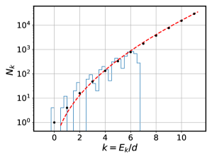
Figure 1: Spectrum of many-body configurations in the uniform model. Here, the total $K$ quantum number of the system is restricted to $K=0$. $N_{k}$ denotes the number of configurations at the excitation energy $E^{*}=kd$. The filled circles and the histogram show the non-interacting and the interacting spectra, respectively. The dotted red curve shows a fit to the functional form $\log(N_{k})\sim\sqrt{k}$.

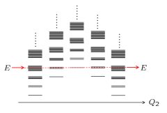
Figure 2: The vertical towers of levels are the $Q$-blocks in the basis of configurations. They are ordered by deformation $Q_{2}$. $E$ is the incident energy for a fission reaction.

Its functional form agrees well with the leading behavior of the Fermi-gas level density formula bm1 as described in the figure caption. The histogram shows the level density after including $\hat{H}_{v}$ in the Hamiltonian of the $Q$-block.

The parameter $d$ will be left unspecified below. It can vary greatly due to shell effects, but in the actinide nuclei it is in the range $0.4-0.5$ MeV Supp . The levels at the neutron emission threshold would then correspond to $k\approx 13-16$ in excitation energy and somewhat higher $k\approx 17$ in level density. What we have described here is a single-reference basis of configurations. Fission requires large-amplitude shape changes, which cannot be reasonably treated in a single-reference basis. As a minimum, one needs to extend the space by including as reference states the local DFT minima across the saddle point of the barrier barranco90 . In fact there are many such minima along typical fission paths be19a . In our model we organize the reference configurations as a chain along a path of increasing deformations, as depicted in Fig. 2. One complication at this point is that the resulting basis may not be orthogonal. We shall come back to this point later.

Model nucleon-nucleon Hamiltonians. In the quasiparticle representation, there are three kinds of two-particle interaction. The interactions that are diagonal in quasiparticle occupations factors are taken into account in $E_{\rm gs}$, the ground state energy of the reference configuration. The interactions changing the orbital of one of the nucleons do not contribute in the reference configuration if it is a stationary state of the DFT; otherwise it induces a diabatic transformation of the configuration. Such transformations are generally unfavored on energetic grounds no83 and they are omitted in the present model. We are left with the interactions that change the orbitals of both particles. In this Letter we deal only with the neutron-proton interaction. The pairing interaction between identical particles is certainly important as well; in fact, it is likely to be more important in non-diabatic collective dynamics ha20-2 ; ro14 . However, it is also important to assess the effects of the residual neutron-proton interaction BBB92 , and this has not be done until now.

We write the interaction Hamiltonian as

$$\hat{H}_{v}=v_{\rm np}{\sum}^{\prime}r\,\hat{a}^{\dagger}_{\alpha_{1}}\hat{a}^{\dagger}_{\alpha_{2}}\hat{a}_{\alpha_{3}}\hat{a}_{\alpha_{4}}.$$ (3)

where the parameter $v_{\rm np}$ is the strength of the interaction and $r$ is a random variable from a Gaussian ensemble of unit variance. The summation is over the four $\alpha$ indices restricted to a fixed $Q$ in $\hat{H}_{v}$ and to neighboring $Q$-blocks BBB92 ; CB92 ; be20 ; ha20 ; ha20-2 ; barranco90 in $\hat{H}^{\rm od}_{v}$. Also, the sum is restricted to $\alpha$ sets satisfying $K_{1}+K_{2}=K_{3}+K_{4}$. The assumption that the neutron-proton interaction is Gaussian distributed is certainly not justified for the low-energy states in a $Q$-block where collective excitations can be built up. However, high in the spectrum where only the overall interaction strength is important the mixing approaches the random matrix limit. The strength can be determined by sampling with more realistic interactions that could range in sophistication from simple contact interactions or separable interactions to those used in present-day shell model Hamiltonians. The strength of neutron-proton contact interactions for shell model Hamiltonians is typically in the range $250-500$ MeV-fm³ BBB92 ; yoshida13 . The corresponding strength in actinides Supp for our parameterization is $0.05d-0.1d$; we take $v_{\rm np}=0.05d$ in most of the examples below.

The configurations may be characterized by the number of quasiparticles as well as by the energy index $k$. Each $k\neq 0$ subblock contains configurations going from two quasiparticles to the maximum energetically allowed. The subblocks are all connected by the residual interaction, although the matrices connecting them are sparse. For example, the $N_{6}\times N_{6}$ matrix has an off-diagonal filling of 5%, while the $N_{6}\times 1$ matrix connecting the $k=6$ subblock to the ground state is 27% filled.

In the presence of the residual interaction, the eigenstates of a shell-model configuration space are found to approach the random matrix limit of the Gaussian Orthogonal Ensemble (GOE) when the rms interaction strength is larger than the level spacing between configurations gu89 ; wei09 . For reaction theory, the most important GOE characteristic is the Porter-Thomas distribution of decay widths, requiring a nearly Gaussian distribution of configuration amplitudes in the eigenstates. The eigenstates of large-dimension $k$-subblocks do in fact acquire the properties of the GOE, even though the sparseness of the interaction matrix works against a complete mixing of the configurations Supp . More realistic model that do not permit the $k$ grouping will still approach the GOE at high excitation energy. However, it should be mentioned that a numerical study br84 ; zel96 of a light-nucleus spectrum did not confirm the above stated criterion for GOE behavior.

The interaction between $Q$-blocks is responsible for shape changes BBB92 and is thus crucial to the modeling. It is clear that the interaction is somewhat suppressed due to the imperfect overlap of orbitals built on different mean-field reference states. Another complication is that the configurations in different $Q$-blocks will not be orthogonal unless special measures are taken, e.g., restriction by $K$-partitioning be17 . These problems have long been dealt with in other areas of physics lo55 ; re11 ; ro20 and can be treated in nuclear physics in the same way. For our model, we simply parameterize the effects by the attenuation factor $f_{\rm od}$ in Eq. (1).

Reaction theory. Induced fission is in the domain of reaction theory: an external probe, typically a neutron, excites the nucleus leading to its decay by fission. A number of reaction-theoretic formalisms are available for treating CI Hamiltonians. We mention in particular the $K$-matrix formalism be20 ; KTW15 ; BK17 ; al20 ; al21 and the $S$-matrix formalism KTW15 ; thompson09 . The key quantity is the transmission coefficient from an incoming channel to the decay channels of interest,

$$T_{{\rm in},C}=\sum_{j\in C}|S_{{\rm in},j}|^{2}.$$ (4)

Here $C$ is the set of quantum mechanical channels associated with the type of reaction. For neutron-induced reactions on heavy nuclei, it could be inelastic scattering, capture, or fission. The relevant $S$-matrix quantities may be calculated as da01 ; al21

$$|S_{j,j^{\prime}}|^{2}=\sum_{\mu,\mu^{\prime}}\Gamma_{j,\mu}|(\tilde{H}-E)^{-1}|^{2}_{\mu,\mu^{\prime}}\Gamma_{j^{\prime},\mu^{\prime}}.$$ (5)

Here $\Gamma_{i,\mu}$ is the decay width of the state $\mu$ into the channel $i$. Note that the CI Hamiltonian $H$ is modified by including of the coupling to the channels. We assume in the model that each channel couples to a single internal configuration, and we neglect dispersive effects. The modified Hamiltonian $\tilde{H}$ then reads,

$$\tilde{H}_{\mu,\mu^{\prime}}=H_{\mu,\mu^{\prime}}-i\delta_{\mu,\mu^{\prime}}\sum_{j}\Gamma_{j,\mu}/2.$$ (6)

The main observable we are interested in is the branching ratio between fission and capture. We define it as

$$B_{\rm cap,fis}=\frac{\int dE\,T_{{\rm in},{\rm fis}}}{\int dE\,T_{{\rm in},{\rm cap}}}.$$ (7)

The range of integration is the same for numerator and denominator and in practice would be determined by experimental considerations. For simplicity, we assume that the entrance channel width is small compared to the decay widths, in which case it cancels out of Eq. (7). For a typical example the experimental quantities are $\Gamma_{\rm cap}\approx 0.04$eV and $B_{\rm cap,fis}\approx 3$ BK17 .

Results. We can now set the parameters to simulate the branching between capture and fission processes. To this end, we consider chains of three or more $Q$-blocks; the first represents the spectrum built on the ground state and the last has the doorway state to fission channels. Imaginary energies $-i\Gamma_{\rm cap}/2$ and $-i\Gamma_{\rm fis}/2$ are added to the blocks in $\tilde{H}$ to account for the decay widths be20 .

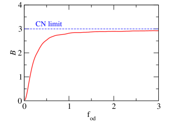
Figure 3: The branching ratio as a function of the attenuation factor $f_{\rm od}$ in the interaction between $Q$-blocks. The model space is $(k=0-4)\times 3$ and the reference-state energies are $E_{\rm gs}=(0.0,0.0,0.0)$. Other parameters are: $v_{\rm np}=0.05d$, $\Gamma_{\rm cap}=0.001d$, and $\Gamma_{\rm fis}=0.003d$. The energy average in Eq. (7) is taken in the range of $3.5d\leq E\leq 4.5d$. The dashed line denotes the branching ratio in the compound nucleus limit, $B_{\rm cap,fis}=\Gamma_{\rm fis}/\Gamma_{\rm cap}=3.0$.

As a warm-up, we find conditions on $f_{\rm od}$ that justify the compound-nucleus (CN) hypothesis that the relative decay rates are proportional to the decay widths in $\tilde{H}$. The model has three identical $Q$-blocks composed of $k\leq 4$ subblocks. The calculated branching ratios are shown in Fig. 3. Note that the stochastic treatment of the interaction in Eq. (3) produces a distribution of ratios; only one of them is shown in the figure. For $f_{\rm od}\gtrsim 1$, the branching ratio is consistent with the formula $B_{\rm cap,fis}=\Gamma_{\rm fis}/\Gamma_{\rm cap}$, confirming the CN limit. Even with $f_{\rm od}=0.5$, the branching ratio is only $15$% less than the CN limit.

We next impose a barrier and examine the fundamental assumption of present-day theory of induced fission, namely that near the barrier top the decay rate is by the Bohr-Wheeler (BW) transition state formula BW39 ; B91

$$\Gamma_{\rm BW}=\frac{1}{2\pi\rho}\sum_{i}T_{i}.$$ (8)

Here $i$ are states on the barrier top, $T_{i}$ are transmission coefficients across the barrier, and $\rho$ is the level density of the compound nucleus (i.e., the first $Q$-block) at the given excitation energy. Notice that the BW formula does not depend on the fission widths $\Gamma_{\rm fis}$, unlike Eq. (5).

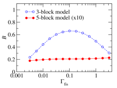
Figure 4: Sensitivity of the branching ratio to the exit channel widths. The blue open circles are for the model space of $(k=0-6)\times 3$ with $E_{\rm gs}=(0,6d,0)$, while the red filled circles are for $(k=0-6)\times 5$ with a parabolic barrier $E_{\rm gs}=(0.0,4.5,6.0,4.5,0.0)$. Other parameters are: $v_{\rm np}=0.05d$, $f_{\rm od}=1.0$, and $\Gamma_{\rm cap}=0.01d$. The incoming channel is assumed to be one of the configurations at $E^{*}=6d$ in the first block, and the energy average in Eq. (7) is taken in the range of $5.5d\leq E\leq 6.5d$.

First consider the model space of 3 identical $Q$-blocks composed of $k\leq 6$ subblocks, with $E_{\rm gs}=(0,6d,0)$ to make a barrier at the middle block. As may be seen in Fig. 4, this model fails the first assumption: the derived branching ratio is sensitive to the fission decay width, $\Gamma_{\rm fis}$. The reason is that there are many virtual transitions possible through the higher levels in the barrier-top $Q$-block. Because the effective number of partially open channels is large, the communication between the end $Q$-blocks remains strong.

We found two ways to greatly diminish the dependence on $\Gamma_{\rm fis}$ in our model. The first way is to increase the chain of $Q$-blocks on the barrier. Then the path across the barrier requires multiple virtual transitions, resulting in a much stronger suppression factor. This may be seen in Fig. 4 for the 5-block case.

The other way is to eliminate the virtual transitions at the barrier by cutting off the spectrum of the middle block. Fig. 5 shows the results with 3 Q-blocks. The first and the last blocks are defined as usual in the $N_{k}$ space. The middle block has only a $k=0$ configuration, shifted in energy to $E_{\rm qp}=k\,d$. The filled circles and the open circles show the branching ratios with $\Gamma_{\rm fis}$ = $0.3d$ and $0.1d$, respectively. There is hardly any difference between the two curves.

One can make a crude approximation to the Bohr-Wheeler transition state formula Eq. (8) within the framework of the model. The branching ratio for a single barrier state with a transmission factor $T_{t}=1$ reads $B_{\rm cap,fis}\sim 1/(2\pi\rho\Gamma_{\rm cap})$. The spread of the $k$ subblock with the given parameters is about $d$, resulting in a level density $\rho=N_{k}/d$. This estimate gives the reasonable agreement shown by the filled squares in the Figure; it appears that the internal transmission factor for large spaces approaches $T=1$. However, the comparison should not be considered quantitative because the level density of the first $Q$-block is not constant over the energy window accessed by the state in the middle.

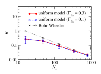
Figure 5: Branching ratios in $(k)/(0)/(k)$ configuration spaces in which the barrier $Q$-block is a single state degenerate with the other $Q$-blocks. Other parameters are $v_{\rm np}=0.05d,~{}f_{\rm od}=1$ and $\Gamma_{\rm cap}=0.01d$. The filled circles and the open circles are obtained with $\Gamma_{\rm fis}=0.3d$ and $0.1d$, respectively. The uncertainties are estimated with 100 different random number sets in the Hamiltonian matrix. The filled squares shows the predicted values from a schematic transition-state formula (see text for details).

Summary and Outlook. The model presented here for induced fission in a CI representation appears to be sufficiently detailed to examine the validity of transition-state theory in a microscopic framework. Depending on the interaction and the deformation-dependent configuration space, one achieves conditions in which branching ratios depend largely on barrier-top dynamics and are insensitive to properties closer to the scission point. The insensitive property is one of the main assumptions in the well-known Bohr-Wheeler formula for induced fission, but up to now it had no microscopic justification.

Whether the transition-state hypothesis is valid under realistic Hamiltonians remains to be seen and will require a large computational effort to answer. In the near term, the model can be applied in a number of different ways. We plan to study the barrier transmission factor $T_{i}$ as a function of barrier height to test another basic assumption in present-day theory, namely treating them by the Hill-Wheeler formula (hi53, , p. 1140). It also appears quite straightforward to include a pairing interaction in the Hamiltonian. This would allow one to explore for the first time the competition between the two kinds of interaction in barrier-crossing dynamics.

This work was supported in part by JSPS KAKENHI Grant Number JP19K03861.

References

- (1) M. Bender et al., J. Phys. G 47, 113002 (2020).
- (2) F. Dönau,J. Zhang and L. Riedinger, Nucl. Phys. A496, 333 (1989).
- (3) B.W. Bush, G.F. Bertsch and B.A. Brown, Phys. Rev. C45, 1709 (1992).
- (4) D. Cha and G.F. Bertsch, Phys. Rev. C46, 306 (1992).
- (5) G.F. Bertsch, Phys. Rev. C 101, 034617 (2020).
- (6) K. Hagino and G.F. Bertsch, Phys. Rev. C 101, 064317 (2020).
- (7) K. Hagino and G.F. Bertsch, Phys. Rev. C 102. 024316 (2020).
- (8) D. Sangalli et al., Phys. Rev. B 93, 195205 (2016).
- (9) A. Bohr and B.R. Mottelson, Nuclear Structure (W.A. Benjamin, Reading, MA, 1969), Vol. I.
- (10) F. Barranco, G.F. Bertsch, R.A. Broglia, and E. Vigezzi, Nucl. Phys. A512, 253 (1990).
- (11) G. F. Bertsch, W. Younes, and L. M. Robledo, Phys. Rev. C 100, 024607 (2019).
- (12) W. Nörenberg, Nucl. Phys. A409, 191 (1983).
- (13) K. Yoshida, Prog. Theor. Exp. Phys. 2013, 113D02 (2013).
- (14) R. Rodríguez-Guzmán and L.M. Robledo, Phys. Rev. C 89, 054310 (2014).
- (15) T. Guhr and H.A. Weidenmüller, Ann. Phys. (N.Y.) 193, 472 (1989).
- (16) H.A. Weidenmüller and G.E. Mitchell, Rev. Mod. Phys. 81, 539 (2009).
- (17) B.A. Brown and G.F. Bertsch, Phys. Lett. B 148, 5 (1984).
- (18) V. Zelvinsky, B.A. Brown, N. Frazier, and M. Horoi, Phys. Rep. 276, 85 (1996).
- (19) G.F. Bertsch, Int. J. Mod. Phys. E 26, 1740001 (2017).
- (20) P.O. Löwdin, Phys. Rev. 97, 1474 (1955).
- (21) M.G. Reuter, T. Seideman, and M.A. Ratner, Phys. Rev. B 83, 085412 (2011).
- (22) J. Rodriguez-Laguna, L.M. Robledo, and J. Dukelsky, Phys. Rev. A 101, 0125105 (2020).
- (23) A.M. Lane and R.G. Thomas, Rev. Mod. Phys. 30, 257 (1958).
- (24) I.J. Thompson and F.M. Nunes, Nuclear Reactions for Astrophysics (Cambridge University Press, Cambridge, 2009).
- (25) T. Kawano, P. Talou, and H.A. Weidenmüller, Phys. Rev. C 92, 044617 (2015).
- (26) G.F. Bertsch and T. Kawano, Phys. Rev. Lett. 119, 222504 (2017).
- (27) Y. Alhassid, G.F. Bertsch, and P. Fanto, Ann. Phys. (N.Y.) 419, 168233 (2020).
- (28) Y. Alhassid, G.F. Bertsch, and P. Fanto, Ann. Phys. (N.Y.) 424, 168381 (2021).
- (29) P.S. Damle, A.W. Ghosh, and S. Datta, Phys. Rev. B 64, 201403 (2001).
- (30) N. Bohr and J.A. Wheeler, Phys. Rev. 56, 426 (1939).
- (31) G.F. Bertsch, J. Phys.: Cond. Matt. 3, 373 (1991).
- (32) D.L. Hill and J.A. Wheeler, Phys. Rev. 89, 1102 (1953).
- (33) See Supplemental Material for the estimates of physical parameters and codes to generate data points in the Figures. It also contains some additional examples.