Quantum metrology with precision reaching beyond-$1/N$ scaling through $N$-probe entanglement generating interactions

Abstract

Nonlinear interactions are recognized as potential resources for quantum metrology, facilitating parameter estimation precisions that scale as the exponential Heisenberg limit of $2^{-N}$. We explore such nonlinearity and propose an associated quantum measurement scenario based on the nonlinear interaction of $N$-probe entanglement generating form. This scenario provides an enhanced precision scaling of $D^{-N}/(N-1)!$ with $D>2$ a tunable parameter. In addition, it can be readily implemented in a variety of experimental platforms and applied to measurements of a wide range of quantities, including local gravitational acceleration $g$, magnetic field, and its higher-order gradients.

I Introduction

Quantum metrology aims at improving the practical measurement precisions via quantum advantages. Various measurement scenarios have been proposed Giovannetti2006 ; Braun2018 ; Giovannetti2011 , capable of achieving precisions beyond the standard quantum limit (SQL) of $1/\sqrt{N}$, or even approach the Heisenberg limit $1/N$ for an ensemble of N particles, with nonclassical probe states, such as the entangled Giovannetti2004 ; Mitchell2004 ; zou2018 ; luo2017deterministic and squeezed states wineland1994squeezed ; Gross2012 ; Bao2020 , as probe states to interferometers. Besides the nonclassical probe states, quantum parameterization processes based on nonlinear interactions between the probes and the to-be-measured (TBM) system, can also improve the precision by amplifying the phase imprinted by the TBM quantity to the probes. For instance, the nonlinear $k$-body interaction can reach a precision scaling of $N^{-k}$ ($N^{-k+\frac{1}{2}}$), with (without) entanglement of the probe PhysRevA.72.045801 ; PhysRevLett.98.090401 ; PhysRevA.77.053613 ; Napolitano2011interaction-based ; NIE2018469 , and the nonlinear $N$-body entanglement generating interaction can even achieve an exponential Heisenberg limit of $2^{-N}$ for measuring its interaction strength roy2008exponentially . These studies support higher than SQL scaling with $N$ for the precision and are broadly applicable.

Despite that the quantum measurement schemes based on the nonlinear interactions can provide the precision with the beyond-$1/N$ scaling, they suffer from a common constraint of weak applicability, arising from the facts that, the nonlinear interaction coupling the TBM system with the probes is hard to engineer, and more severely, the enhanced precision scaling only works for the measurement of the nonlinear interaction strength, which cannot be assigned to an arbitrary TBM quantity. In order to circumvent the constraint, we propose a new nonlinear measurement scheme, which can generalize the beyond-$1/N$ precision scaling to measurements of a wider range of quantities. Instead of introducing a nonlinear interaction between the probes and the TBM system, this measurement scheme deploys the $N$-body entanglement generating interaction to locally couple $N$ probes, and we will simply call it $N$-probe entanglement generation (NPEG) interaction scheme. It will be demonstrated that, for one thing, this NPEG-based scheme maintains the beyond-$1/N$ precision scaling, and more importantly, once the NPEG interaction is engineered, the nonlinearly coupled probes can be associated to various TBM systems and realize the measurements of different TBM quantities with the improved precision.

The engineering of the NPEG interaction can benefit from the highly developed investigations on effective Hamiltonian engineering. Earlier studies on effective Hamiltonian engineering have been carried out on various platforms, especially in ultracold atomic ensembles for generating effective coupling channels between intrinsically isolated states and tuning the coupling strength. The effective coupling channels are usually engineered via either applying external couplings through lasers PhysRev.175.453 ; RevModPhys.76.1037 ; PhysRevX.4.031027 ; RevModPhys.89.011004 , or by tailoring higher order processes intermediated by energetically detuned states PhysRevLett.85.3987 ; PhysRevLett.89.090401 ; dai2017four-body ; Brown540 . Particularly, nonlinear interactions have been proposed and even experimentally realized PhysRevLett.89.090401 ; paredes2008minimum ; nascimbene2012experimental ; Brown540 ; dai2017four-body for the investigations of e.g. quantum simulations, which could be directly applied for the NPEG-based measurements. The studies on effective Hamiltonian engineering help to lay solid foundation to the NPEG-based measurements, which in turn provide new applications to the engineering studies.

This paper is organized as follows: in section II the NPEG-based measurement scheme is introduced, with an intuitive illustration on the precision scaling; in section III the performance of the NPEG-based measurement scheme, in terms of the precision scaling, the time resource, the robustness, is analyzed with the quantum and classical Fisher informations; in section IV, the applicability of the scheme is investigated with a variety of experimentally realizable setups of the measurement scheme; a summary is present in section V.

II NPEG measurement scheme

The key element of the proposed measurement scheme is the NPEG nonlinear interaction, which can be engineered through higher-order processes on various setups PhysRev.175.453 ; RevModPhys.76.1037 ; PhysRevX.4.031027 ; RevModPhys.89.011004 ; PhysRevLett.85.3987 ; PhysRevLett.89.090401 ; PhysRevLett.95.040402 ; paredes2008minimum ; nascimbene2012experimental ; Brown540 ; dai2017four-body . We briefly illustrate the engineering procedure with the example of a bosonic system composed of $N$ identical bosons, where each boson can only occupy two states, denoted by $|a\rangle$ and $|b\rangle$. The Hamiltonian of the original system is

$$H_{\mathrm{org}}=\frac{U}{2}(\hat{a}^{\dagger}\hat{a}^{\dagger}\hat{a}\hat{a}+\hat{b}^{\dagger}\hat{b}^{\dagger}\hat{b}\hat{b})+j(\hat{a}^{\dagger}\hat{b}+\hat{a}\hat{b}^{\dagger})-\frac{\delta_{\mathrm{0}}}{2}(\hat{n}_{a}-\hat{n}_{b}),$$ (1)

in which $\hat{a}/\hat{b}$ ($\hat{a}^{{\dagger}}/\hat{b}^{{\dagger}}$) annihilates (creates) a boson in the state $|a\rangle/|b\rangle$, and $\hat{n}_{a}=\hat{a}^{{\dagger}}\hat{a}$ ($\hat{n}_{b}=\hat{b}^{{\dagger}}\hat{b}$). In the strong interaction regime with $j\ll U$, the interaction of bosons divides the Hilbert space into a set of subspaces, each of which is composed of energetically resonant basis states of fixed integer number of atoms $N=n_{\mathrm{a}}+n_{\mathrm{b}}$. The states $\{|N,0\rangle\!:=|\!\!\Uparrow\rangle,\,|0,N\rangle\!:=|\!\!\Downarrow\rangle\}$ span such a subspace $\mathbb{S}$, which denote states of all bosons confined in the mode $|a\rangle$ and $|b\rangle$, respectively. Within $\mathbb{S}$, $|\!\!\Uparrow\rangle$ and $|\!\!\Downarrow\rangle$ are not directly coupled by $H_{\mathrm{org}}$, but an effective coupling between the two states can be engineered through the higher-order process induced by the single-particle hopping $j$. The resulting effective Hamiltonian (see appendix A for details) within $\mathbb{S}$ reads

$$H_{\mathrm{eff}}\!=\!J_{\mathrm{eff}}\left(|\!\!\Uparrow\rangle\langle\Downarrow\!\!|+|\!\!\Downarrow\rangle\langle\Uparrow\!\!|\right)-\frac{1}{2}\Delta_{\mathrm{0}}\left(|\!\!\Uparrow\rangle\langle\Uparrow\!\!|-|\!\!\Downarrow\rangle\langle\Downarrow\!\!|\right),$$ (2)

in which the first term is the effective coupling of the nonlinear NPEG form, with $J_{\mathrm{eff}}=\frac{NU}{D^{N}(N-1)!}$ $(D=U/j)$, and the second term is induced by the single-particle detuning with $\Delta_{\mathrm{0}}=N\delta_{\mathrm{0}}$. While such NPEG interactions have been widely investigated in various fields S.F2007 ; Dai2016 ; PhysRevLett.85.3987 ; dai2017four-body ; PhysRevLett.89.090401 , for the purpose of e.g. quantum simulations, here we propose that they are also helpful to quantum measurements with improved precision.

The NPEG-based measurement scheme is based on the dynamical process of the many-body correlation induced tunneling (MBCIT), which is a special type of correlated tunneling generalized from the single-particle correlation induced tunneling  refId0 ; CAO2017303 . During the dynamical process, the system periodically oscillate between the initial and the corresponding target, for instance between the state $|+\rangle:=(|\!\!\Uparrow\rangle+|\!\!\Downarrow\rangle)/\sqrt{2}$ and $|\!\!\Downarrow\rangle$. Defining $\Gamma:=\Delta_{\mathrm{0}}/J_{\mathrm{eff}}$, the probability to be in the state $|\!\!\Downarrow\rangle$ during MBCIT from the initial state of $|+\rangle$ is

$$P_{\mathrm{\Downarrow}}(t)=\frac{1}{2}+\frac{\Gamma-\Gamma\cos(\omega t)}{4+\Gamma^{2}},$$ (3)

with $\omega=\sqrt{4J_{\mathrm{eff}}^{2}+\Delta_{\mathrm{0}}^{2}}$. The maximum tunneling amplitude $P^{\max}_{\mathrm{\Downarrow}}=\frac{(2+\Gamma)^{2}}{2(4+\Gamma^{2})}$ is reached at the half period, which builds up a dependence between $\Delta_{\mathrm{0}}$ and the experimentally accessible observable $P^{\max}_{\mathrm{\Downarrow}}$. Such dependence permits the estimation of $\Delta_{\mathrm{0}}$, and equivalently $\delta_{\mathrm{0}}$, through the measurement of $P^{\max}_{\mathrm{\Downarrow}}$. The derivative $\partial_{\Delta_{\mathrm{0}}}P^{\max}_{\mathrm{\Downarrow}}$ determines the precision of the estimation, and shows a beyond-exponential dependence on the number of bosons $N$, implying a beyond-$1/N$ scaling of the estimation precision. In Fig. 1(a), the temporal evolutions of $P_{\mathrm{\Downarrow}}(t)$ are depicted for different detunings, and the dependence of the tunneling amplitude on the detuning is illustrated. The MBCIT can also be viewed as an effective precession on the Bloch sphere spanned by $\{|\!\!\Downarrow\rangle,|\!\!\Uparrow\rangle\}$, as shown in Fig. 1(b), in which $H_{\mathrm{eff}}$ plays the role of a biased magnetic field.

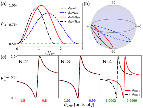
Figure 1: (a) Time evolution of the probability $P_{\Downarrow}$ with the initial state $|+\rangle$ for the total detuning $\Delta_{\mathrm{0}}=0$ (dotted green line), $\Delta_{\mathrm{0}}=J_{\mathrm{eff}}$ (dashed blue line), $\Delta_{\mathrm{0}}=2J_{\mathrm{eff}}$ (solid red line) and $\Delta_{\mathrm{0}}=3J_{\mathrm{eff}}$ (dash-dotted black line). (b) Schematic of evolution trajectories for the initial state $|+\rangle$ with the values of $\Delta_{\mathrm{0}}$ discussed in (a) (lines of the same color correspond to the same value of $\Delta_{\mathrm{0}}$). (c) The maximum tunneling amplitude $P^{\max}_{\mathrm{\Downarrow}}$ as a function of $\delta_{\mathrm{CMP}}$ under slightly different values of $\delta_{\mathrm{TBM,1}}$ and $(1+10^{-4})\delta_{\mathrm{TBM,1}}$ for $N=2$ (left panel), $N=3$ (middle panel) and $N=4$ (right panel). Here $\delta_{\mathrm{TBM,1}}$ is assumed to take the same value of $j$ ($j$ is set to be 1).

The NPEG-based measurement scheme takes each boson in the two-mode system as a probe for measuring the detuning (of some TBM system), specified as $\delta_{\mathrm{TBM}}$ in the following. Benefiting from the sharp particle-number dependence of $\partial_{\Delta_{\mathrm{0}}}P^{\max}_{\mathrm{\Downarrow}}$ in the MBCIT process, a precision beyond-$1/N$ scaling is achieved. Further optimization of the scheme with respect to the value of the detuning itself can also affect the precision, and this optimization is carried out by introducing a compensating of the single-particle detuning, with strength $\delta_{\mathrm{CMP}}$, to maximize the measurement precision of $\delta_{\mathrm{TBM}}$. The total single-particle and many-body detunings, namely $\delta_{\mathrm{0}}$ and $\Delta_{\mathrm{0}}$, respectively, are then composed of the TBM and the compensate ones, and the TBM detuning can be estimated by $\delta_{\mathrm{TBM}}=\delta_{\mathrm{0}}-\delta_{\mathrm{CMP}}$, where the total detuning is deduced from the measured $P^{\max}_{\mathrm{\Downarrow}}$. Provided that the value of $\delta_{\mathrm{CMP}}$ can be obtained with a high enough precision, the precision of $\delta_{\mathrm{TBM}}$ is determined also to a high precision by that of $P^{\max}_{\mathrm{\Downarrow}}$, which can be optimized by tuning $\delta_{\mathrm{CMP}}$.

For a fixed $\delta_{\mathrm{TBM}}$, the $\delta_{\mathrm{CMP}}$ is scanned and the corresponding $P^{\max}_{\mathrm{\Downarrow}}$ is measured, from which the total detuning with the highest precision is deduced. Figure. 1(c) plots the response of $P^{\max}_{\mathrm{\Downarrow}}$ to $\delta_{\mathrm{CMP}}$ in the presence of two slightly different TBM detunings $\delta_{\mathrm{TBM,1}}$ (red solid lines) and $\delta_{\mathrm{TBM,2}}=(1+10^{-4})\delta_{\mathrm{TBM,1}}$ (black dashed lines) for different probe number of $N=2$ (left panel), $N=3$ (middle panel), and $N=4$ (right panel). As calibrated by the colored tick-marks on the $x$-axis, the response grows sharply as $N$ increases, indicating that the NPEG measurement scheme indeed provides a significant precision improvement with increasing probe number. Meanwhile, it shows that only with $N=4$ probes can distinguish the two slightly different TBM detunings via statistics from the measured state populations, indicating that the NPEG-based scheme can also enhance measurement resolution. The precision and the resolution with enhanced scaling over the number of probes will benefit realistic metrological scenarios such as gravity and its gradient.

The NPEG-based measurement described above is designed based on a different mechanism from the proposal in Ref. roy2008exponentially and provides enhanced precision scaling as well as a broader applicability. Since the uncertainty of parameter estimation can be determined by $\Delta\delta=\Delta P/|\partial_{\delta}P|$, where $\Delta\delta$ and $\Delta P$ refer to the uncertainties of the estimated parameter $\delta$ and the experimentally measured probability $P$, respectively, the NPEG-based scheme can simultaneously improve $\Delta P$ and $|\partial_{\delta}P|$, and consequently provides a new precision scaling, as will be demonstrated below. Moreover, in the NPEG-based scheme, once the nonlinear interaction between the probes is realized, the nonlinearly coupled probes can be subjected to different TBM systems and measure different quantities, enabling broad practical applicability of the nonlinear interactions as the quantum resource.

III Optimization and characterization

The precision of the NPEG-based measurement can be analyzed and optimized according to the Quantum Cramér-Rao bound Helstrom1976 ; Holevo1982 , one of the most well-studied bounds in quantum metrology for both single- Paris2009 ; Toth2014 and multi-parameter Szczykulska2016 ; Liu2020 estimations. In this theory, the standard deviation $\delta\delta_{0}$ is bounded by the inverse of the classical and quantum Fisher information (CFI and QFI), denoted by $F_{\mathrm{c}}$ and $F_{\mathrm{q}}$, respectively. In the NPEG-based measurement sheme, the maximized CFI and the corresponding precision of $\delta_{\mathrm{0}}$ can be analytically derived as (see appendix B for details)

$$\begin{split}F_{\mathrm{c,opt}}&=\frac{1}{J^{2}_{\mathrm{eff}}}=\left(\frac{D^{N}(N-1)!}{NU}\right)^{2},\\ \delta\delta_{\mathrm{0}}&=\frac{\delta\Delta_{\mathrm{0}}}{N}=\frac{U}{D^{N}(N-1)!},\end{split}$$ (4)

indicating the beyond-$1/N$ scaling of the precision on the number of probes. The maximized $F_{\mathrm{c,opt}}$ is reached at $(\Delta_{\mathrm{0}},\omega t)=(0,\pi)$, with the probe state $\cos\frac{\theta}{2}|\!\!\Uparrow\rangle+\sin\frac{\theta}{2}|\!\!\Downarrow\rangle$ $(\theta\in[0,\pi])$, which lies on the longitude line connecting the states $|\pm\rangle$ in the Bloch sphere. To further check whether the measurement $\{|\!\!\Downarrow\rangle\langle\Downarrow\!\!|,|\!\!\Uparrow\rangle\langle\Uparrow\!\!|\}$ is optimal, the QFI under the same condition of the maximized CFI can be derived as:

$$F_{\mathrm{q,opt}}=\frac{1}{J^{2}_{\mathrm{eff}}}=\left(\frac{D^{N}(N-1)!}{NU}\right)^{2},$$ (5)

which coincides with $F_{\mathrm{c,opt}}$, meaning that the MBCIT scheme is an optimal measurement scheme to achieve the ultimate theoretical precision limit, with a beyond-$1/N$ scaling behavior PhysRevLett.72.3439 .

The scaling in Eqs. (4) and (5) is restricted to $\Delta_{\mathrm{0}}=0$, and corresponds to the local precision PhysRevX.2.041006 , which at first sight might seem to limit the applicability of the NPEG-based scheme. The compensate detuning introduced actually circumvents this restriction. If the compensate detuning can be controlled to high precision, it is always possible to shift the total detuning to $\Delta_{\mathrm{0}}=0$ with a fixed $\Delta_{\mathrm{TBM}}$, and maintain the overall optimal beyond-$1/N$ scaling across all regions. To avoid the high prior information paradox on $\delta_{\mathrm{TBM}}$, as discussed in Ref. Giovannetti2012 , in practice this process needs to be performed adaptively, such as performing a rough pre-estimation in advance Berni2015 . We will demonstrate with practical examples to show that this prerequisite of the compensate potential with the high controllability can be fulfilled in various practical circumstances and the performance of nonzero $\Delta_{0}$ will also be thoroughly discussed.

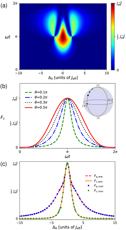
Figure 2: (a) The CFI $F_{\mathrm{c}}$ as a function of total detuning $\Delta_{0}$ and $\omega t$ for the initial state $|+\rangle$. (b) Time evolution of $F_{\mathrm{c}}$ for the initial states $\sin(\frac{\theta}{2})|\!\!\Uparrow\rangle+\cos(\frac{\theta}{2})|\!\!\Downarrow\rangle$ with $\theta=0.1\pi$ (dashed green line), $\theta=0.2\pi$ (dash-dotted blue line), $\theta=0.3\pi$ (dotted black line) and $\theta=0.5\pi$ (solid red line). The insert plot shows the position of these states on the Bloch sphere. (c) The maximum CFI $F_{\mathrm{c}}$ and QFI $F_{\mathrm{q}}$ as a function of $\Delta_{0}$. The dashed red and solid orange lines are the analytical solutions of $F_{\mathrm{q}}$ and $F_{\mathrm{c}}$ derived via Eq. (2), and the blue squares and green stars are the numerical solutions of $F_{\mathrm{q}}$ and $F_{\mathrm{c}}$ calculated with Eq. (1), respectively. Here $N$ is set to be 4.

Apart from the minimum value of the precision, the robustness of the achieved precision against imperfect control during measurement is also an important factor in practical quantum metrology Degen2017 . Figure 2 demonstrates the robustness against deviations to the optimized rescaled measurement time $\omega t$ and the total detuning $\Delta_{\mathrm{0}}$ (Fig. 2(a)), as well as against the initial state in terms of the relative phase $\phi$ (Fig. 2(b)). First, the general behavior of the CFI as functions of $\Delta_{\mathrm{0}}$ and $\omega t$ is given in Fig. 2(a) for the probe state $|+\rangle$. It is seen that at $(\Delta_{\mathrm{0}},\omega t)=(0,\pi)$ $F_{\mathrm{c}}$ reaches the maximum value, and is most stable with respect to the deviations of the detuning and the measurement time. Second, Figure. 2(b) illustrates that for probe states residing on the longitude line of $\varphi=0$, $F_{\mathrm{c}}$ takes the same maximized value, while the line width of $F_{\mathrm{c}}$ as a function of $\omega t$ increases as the probe state approaches $|+\rangle$ (also $|-\rangle$). This indicates that the probe states $|\pm\rangle$ provides the precision of the best robustness with respect to the measurement time. In Fig. 2(c), we further examine $F_{\mathrm{c}}$ and $F_{\mathrm{q}}$ derived from the approximate $H_{\mathrm{eff}}$, with the results numerically calculated by $H_{\mathrm{org}}$. The analytical results based on $H_{\mathrm{eff}}$ are found to coincide with numerically obtained ones from $H_{\mathrm{org}}$, which verifies the validity of the analysis based on $H_{\mathrm{eff}}$ and confirms the engineered nonlinear NPEG interaction as a useful quantum resource. Besides, it also shows that the performance of the scheme is robust to $\Delta_{0}$ as in the plot the CFI for $\Delta_{0}=\pm 0.5$ is around $89.5\%$ of that for $\Delta_{0}=0$, indicating that the scheme can be well performed adaptively.

The interrogation time is also an important criterion for the performance of different measurement schemes Giovannetti2001 ; PhysRevX.8.021022 , thus it is necessary to evaluate how the NPEG interaction benefits the measurement in view of time resource. For this purpose, we compare the time cost to reach the same precision in both linear and nonlinear measurements using the MBCIT process. The linear MBCIT measurement corresponds to loading only a single probe to the measurement procedure and eliminating the nonlinear interaction effect, i.e., taking $N=1$ in the analysis. The ratio of the time cost to reach the same precision for the linear and the $N$-probe nonlinear MBCIT measurements, turns out to be $D^{N-1}(N-1)!$ (see appendix C), which indicates that time cost to reach the same precision also decreases exponentially with $N$.

IV Application scenarios

Besides the beyond-$1/N$ scaling, the NPEG-based measurement scheme also enjoys the advantage of the high flexibility, which allows it to be applied to a wide range of quantities. In this section, we present several experimental setups with ultracold atomic ensembles, on which the NPEG-based scheme can be performed to measure different quantities, such as gravity, magnetic field and its gradients.

Our first example explores a system of ultracold atoms confined in a double-well potential, and various nonlinear interactions have been already discussed and investigated in this setup dudarev2003entanglement ; S.F2007 ; PhysRevLett.100.040401 ; PhysRevLett.107.210405 ; Dai2016 , and the NPEG-based measurement scheme can be directly applied. As indicated in the first row of Fig. 3, the NPEG interaction coupling the two many-body states of atoms confined in the subspace of all in the left or right wells, can be engineered by the interplay between the contact interaction and the single-particle hopping. The NPEG-based measurements of the energy detuning between the two wells can be performed, allowing for estimations of gravity acceleration along the orientation of the double well. As illustrated in the second row of Fig. 3, a second type of NPEG interaction can be engineered between spinor atoms confined in the double-well potential PhysRevLett.85.3987 ; PhysRevLett.89.090401 , and couples the states of, for instance, $|\!\!\Uparrow\rangle=|\!\!\uparrow^{\otimes N},\downarrow^{\otimes N}\rangle$ and $|\!\!\Downarrow\rangle=|\!\!\downarrow^{\otimes N},\uparrow^{\otimes N}\rangle$, where each well is occupied by $N$ atoms, and atoms in different wells are polarized along opposite directions. Such a probe space is insensitive to the net magnetic field and can be used for in-situ measurement of the linear magnetic gradient along the orientation of the potential. In both examples, the highly-controllable lasers forming the double well potential can induce compensating detuning with required precision.

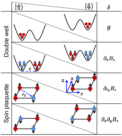
Figure 3: Schematics of the practical platforms discussed in the main text for performing the MBCIT measurements, with the choice of the probe states and the TBM quantities.

The NPEG-based measurement can also be applied to spinor atom plaquette,  paredes2008minimum ; nascimbene2012experimental ; dai2017four-body . In the plaquette, the nonlinear interactions of the NPEG form are realized within different energetically resonant subspaces of the plaquette system, and each such subspace provides a probe space $\mathbb{S}$ for the NPEG-based measurement scheme. The last two rows of Fig. 3 present two probe spaces capable of measuring the magnetic gradients of different orders. In the configuration that the spin plaquette lies in the $xy$ plane and the TBM magnetic field polarized along the $z$-axis, denoted by $B_{z}(\vec{r})$, the probe space spanned by $\{|\!\!\uparrow\downarrow\uparrow\uparrow\rangle,|\!\!\uparrow\uparrow\uparrow\downarrow\rangle\}$ (indicating the polarization of the four spinors in the plaquette), allows the in-situ measurement of the first-order magnetic gradient $\partial_{\hat{r}_{0}}B_{z}$, with $\hat{r}_{0}$ along the diagonal line of the plaquette (slashed line in the third row of Fig. 3. Turning to the probe space of $\{|\!\!\uparrow\downarrow\uparrow\downarrow\rangle,|\!\!\downarrow\uparrow\downarrow\uparrow\rangle\}$, the total spin of the probe states is zero, and such a probe space provides a good candidate for the in-situ measurement of the second-order magnetic gradient $\partial_{x}\partial_{y}B_{z}$. The spin-dependent lattice potential is also readily implemented in the setup, which can induce the single-particle compensate detunning.

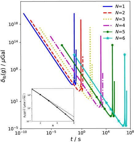
Figure 4: The lower-bound uncertainty $\delta_{{\rm lb}}(g)$ as a function of measurement time $t$ for different particle numbers ($N=1$ to $6$) with $M=10000$ supercells. The parameters are taken from Ref. 2020Sci_Y , with the wavelength of the “short” lattices $\lambda_{s}=767{\rm nm}$, the tunneling $J=50{\rm Hz}$ and the interaction $U=1251{\rm Hz}$. The insert shows $\delta_{{\rm lb}}(g)\sqrt{t}$ as a function of $N$, in which the dotted line presents an exponentially decaying curve.

We further take the measurement scenario introduced in the first row of Fig. 3 as an example to quantitatively analyze the performance of the NPEG-based scheme in the practical measurements. We consider an array of double wells, each of which is loaded with $N$ ultracold atoms as the probe. The atoms are subjected to the gravity force and the gravity acceleration $g$ of the Earth is the TBM quantity. In the measurement setup, we consider that the NPEG-based measurements are performed in parallel for $M=10000$ double-well supercells. We calculate the lower-bound uncertainty of measured $g$ as a function of the measurement time $t$ for $N\in[1,6]$, with all relative parameters taken from the experimental setup in Ref. 2020Sci_Y . As shown in the main figure of Fig. 4, the lower-bound uncertainty $\delta_{{\rm lb}}(g)$ monotonically decreases with the measurement time, until reaching a minimum. The minimized $\delta_{{\rm lb}}(g)$ corresponds to the optimized Fisher information derived in Eqs. (4) and (5), and the measurement time reaching this minimum is just the optimal measurement time. Moreover, as shown in Fig. 4, increasing $N$, on the one hand, can exponentially suppress $\delta_{{\rm lb}}(g)$, and on the other, it increases the measurement time, which bring in a competition in the practical measurements between minimizing the uncertainty and shortening the measurement time. Current experiments on the ultracold atomic dynamics can reach a coherent time over $10$ s, and setting the measurement time on this order, one can find that $N=3$ provides the best lower-bound uncertainty approaching $10\,\mu$Gal, which confirms the NPEG scheme as a source of high precision measurements. Furthermore, assuming that the dynamical coherence time of lattice ultracold atomic experiments can approach the order of $10^{3}$ s in the near future, measurements in a double-well array containing $M=10000$ supercells with each confining $N=4$ bosons provides the measurement uncertainty below $1\,\mu$Gal. In the insert of Fig. 4, we further plot $\delta_{{\rm lb}}(g)\sqrt{t}$ as a function of $N$, which is a joint measure of the performance with respect to the precision and the time resource. The result illustrates that $\delta_{{\rm lb}}(g)\sqrt{t}$ decreases (beyond-)exponentially with $N$, which further confirms the beyond-$1/N$ scaling in the joint viewpoint of precision and the time resource.

The highly developed controllability of ultracold atomic ensembles can facilitate the flexible engineering of the NPEG-type interaction and the compensating detuning with the required precision. The isolation of atomic ensembles from their environment can further suppress the noise induced decoherence to a great extent, and guarantees the long enough coherence time for the proposed measurement PhysRevLett.79.3865 .

V Summary and discussion

We have explored the NPEG interaction as a resource for quantum measurement, and proposed the measurement scheme based on the NPEG-induced MBCIT dynamics. We have demonstrated that, (i) the NPEG nonlinear interaction manifest itself as a novel measurement resource, which provides an improved precision limit with the beyond-$1/N$ scaling of $1/(D^{N}(N-1)!)$; (ii) the measurement scheme based on the MBCIT process provides a practical and optimal measurement scheme to achieve the beyond-$1/N$ scaling.

The NPEG-based measurement scheme not only provides a new mechanism to invoke nonlinearity and leads to a new type of scaling behaviors, its high applicability, as illustrated by the ultracold atomic ensemble, magnetic molecules 1980carboxylate ; 1984Hydrolysis and nuclear-magnetic-resonance setups PhysRevA.66.044308 , also facilitate the development of next-generation high-precision apparatuses like gravimeters and magnetometers and benefit both the fundamental and applied science.

Appendix A The effective Hamiltonian

The system of $N$ Bosons in a double-well trap can be described by a two-mode single-band Bose-Hubbard Hamiltonian:

$$H_{\mathrm{org}}=\frac{U}{2}(\hat{a}^{\dagger}\hat{a}^{\dagger}\hat{a}\hat{a}+\hat{b}^{\dagger}\hat{b}^{\dagger}\hat{b}\hat{b})+j(\hat{a}^{\dagger}\hat{b}+\hat{a}\hat{b}^{\dagger})-\frac{\delta_{\mathrm{0}}}{2}(\hat{n}_{a}-\hat{n}_{b}),$$ (6)

in which $\hat{a}^{({\dagger})}/\hat{b}^{({\dagger})}$ annihilates (creates) a particle in the state $|a\rangle/|b\rangle$, and $\hat{n}_{a}=\hat{a}^{{\dagger}}\hat{a}$ ($\hat{n}_{b}=\hat{b}^{{\dagger}}\hat{b}$). In the regime of strong interaction $j\ll U$, the first term of $H_{\mathrm{org}}$ denotes the interaction of particles, which divides the complete Hilbert space into different energetically off-resonant subspaces $\{|N-m,m\rangle\!,\,\leavevmode\nobreak\ |m,N-m\rangle\!\}$, while each subspaces composed of basis states energetically in resonance with each other. The second term is the one-body hopping term, which builds up higher-order couplings between basis states in each subspace. The last term denotes the energy detuning between $|a\rangle$ and $|b\rangle$. Taking the subspace $\mathbb{S}$ spanned by $\{|N,0\rangle\!:=|\!\!\Uparrow\rangle,\,|0,N\rangle\!:=|\!\!\Downarrow\rangle\}$, and the two base vectors can not be directly coupled with each other, but only by high-order coupling processes, as demonstrated in Fig. 5 for $N=4$. Actually, all vectors $|N-m,m\rangle$ participate in this high-order coupling processes, and this effective coupling can be evaluated by high-order perturbation theory

$$J_{\mathrm{eff}} = \frac{\prod_{m=0}^{N-1}\langle m,N-m|\hat{H}_{\mathrm{J}}|N-m-1,m+1\rangle}{\prod_{m=1}^{N-1}(\langle 0,N|\hat{H}_{\mathrm{int}}|N,0\rangle\!-\!\langle m,N\!-\!m|\hat{H}_{\mathrm{int}}|N\!-\!m,m\rangle)}$$ (7)

$$= \frac{NU}{D^{N}(N-1)!},$$

where $D=U/j$, $\hat{H}_{\mathrm{J}}$ and $\hat{H}_{\mathrm{int}}$ denotes the hopping and the interaction part of the $H_{\mathrm{org}}$, respectively. Moreover, the third term of $H_{\mathrm{org}}$ induces the detuning between the two vectors $|N,0\rangle$ and $|0,N\rangle$ can be written as $\Delta_{\mathrm{0}}=N\delta_{\mathrm{0}}$ and the engineered Hamiltonian becomes

$$H_{\mathrm{eff}}\!=\!J_{\mathrm{eff}}\left(|\!\!\Uparrow\rangle\langle\Downarrow\!\!|+|\!\!\Downarrow\rangle\langle\Uparrow\!\!|\right)-\frac{1}{2}\Delta_{\mathrm{0}}\left(|\!\!\Uparrow\rangle\langle\Uparrow\!\!|-|\!\!\Downarrow\rangle\langle\Downarrow\!\!|\right).$$ (8)

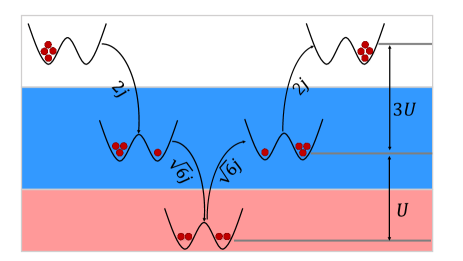
Figure 5: Pathway of the high-order coupling processes in the high-order perturbation theory for $N=4$.

Appendix B Calculations of the CFI

The temporal evolution of the system during the effective Hamiltonian in Eq. (8) for a general probe state of $\cos\frac{\theta}{2}|\!\!\Uparrow\rangle+e^{i\varphi}\sin\frac{\theta}{2}|\!\!\Downarrow\rangle$ ($\theta\in[0,\pi]$, $\varphi\in[0,2\pi]$) is given by $|\psi(t)\rangle=C_{\Uparrow}(t)|\Uparrow\rangle+C_{\Downarrow}(t)|\Downarrow\rangle$, where

$$C_{\Uparrow}(t)$$

$$= \cos\!\left(\frac{\omega t}{2}\right)\!\cos\!\left(\frac{\theta}{2}\right)\!+\!2\mathrm{sgn}(J_{\mathrm{eff}})\frac{\sin(\frac{\theta}{2})\sin(\frac{\omega t}{2})\sin\varphi}{\sqrt{4+\Gamma^{2}}}$$

$$+i\!\left\{\frac{\mathrm{sgn}(J_{\mathrm{eff}})\sin^{2}(\frac{\omega t}{2})}{4+\Gamma^{2}}\!\left[\Gamma\!\cos\!\left(\frac{\theta}{2}\right)\!-\!2\sin\!\left(\frac{\theta}{2}\right)\cos\varphi\!\right]\!\right\},$$

that is to say, the probability of the measurement $\{|\!\!\Downarrow\rangle\langle\Downarrow\!\!|,|\!\!\Uparrow\rangle\langle\Uparrow\!\!|\}$ reads

$$P_{\Uparrow}(t) \!=\! \left[\!\cos\!\left(\!\frac{\omega t}{2}\!\right)\!\cos\!\left(\!\frac{\theta}{2}\!\right)\!\!+\!\!2\,\mathrm{sgn}(J_{\mathrm{eff}})\frac{\sin(\frac{\theta}{2})\sin(\frac{\omega t}{2})\sin\varphi}{\sqrt{4+\Gamma^{2}}}\right]^{2}\!\!$$ (9)

$$+\frac{\sin^{2}(\frac{\omega t}{2})}{4+\Gamma^{2}}\left[\Gamma\cos\left(\frac{\theta}{2}\right)-2\sin\left(\frac{\theta}{2}\right)\cos\varphi\right]^{2},$$

and

$$P_{\Downarrow}(t)=1-P_{\Uparrow}(t),$$ (10)

with $\omega=\sqrt{4J_{\mathrm{eff}}^{2}+\Delta_{\mathrm{0}}^{2}}$ and $\Gamma=\Delta_{\mathrm{0}}/J_{\mathrm{eff}}$.

It is generally known that the classical Fisher information $F_{\mathrm{c}}$ can be obtained via $F_{\mathrm{c}}=\sum_{i}(\partial_{x}p_{i})^{2}/p_{i}$ with $\{p_{i}\}$ a set of probability distribution. For our system,

$$F_{\mathrm{c}}=\frac{(\partial_{\Delta_{\mathrm{0}}}P_{\mathrm{\Uparrow}})^{2}}{P_{\mathrm{\Uparrow}}}+\frac{(\partial_{\Delta_{\mathrm{0}}}P_{\mathrm{\Downarrow}})^{2}}{P_{\mathrm{\Downarrow}}}.$$ (11)

Substitute formula Eq.(9) into formula Eq.(11), we can find that $F_{\mathrm{c}}$ is a function consisting of four parameters $\theta$, $\varphi$, $\omega t$ and $\Delta_{\mathrm{0}}$ and could be written as

$$F_{\mathrm{c}}(\theta,\varphi,\omega t,\Delta_{\mathrm{0}})=\frac{F_{\mathrm{C1}}(\theta,\varphi,\omega t,\Delta_{\mathrm{0}})}{F_{\mathrm{C2}}(\theta,\varphi,\omega t,\Delta_{\mathrm{0}})}.$$ (12)

Here $F_{\mathrm{C1}}(\theta,\varphi,\omega t,\Delta_{\mathrm{0}})$ and $F_{\mathrm{C2}}(\theta,\varphi,\omega t,\Delta_{\mathrm{0}})$ are the numerator and denominator of $F_{\mathrm{c}}$, respectively, and could be expressed as

$$F_{\mathrm{C1}}(\theta,\varphi,\omega t,\Delta_{\mathrm{0}})$$ (13)

$$= 4\Big{\{}2J_{\mathrm{eff}}\Gamma\cos\theta[2\cos(\omega t)-2+(\omega t)\sin(\omega t)]$$

$$+\sin\theta\left[J_{\mathrm{eff}}\cos\varphi(\Gamma^{2}-4)(\cos(\omega t)\!-\!1)\!+\!\Gamma^{2}(\omega t)\sin(\omega t)\right]$$

$$+\Gamma\sqrt{J_{\mathrm{eff}}^{2}(4+\Gamma^{2})}[\sin(\omega t)-\omega t\cos(\omega t)]\sin\varphi)\Big{\}}^{2}\!\!,$$

and

$$F_{\mathrm{C2}}(\theta,\varphi,\omega t,\Delta_{\mathrm{0}})$$ (14)

$$= J_{\mathrm{eff}}^{2}(4+\Gamma^{2})^{2}\Bigg{\{}J^{2}_{\mathrm{eff}}(4+\Gamma^{2})^{2}$$

$$\!-\!\Big{[}J_{\mathrm{eff}}(\Gamma^{2}+4\cos(\omega t))\!\cos\theta\!-\!4J_{\mathrm{eff}}\Gamma\cos\varphi\sin\theta\sin^{2}\!\left(\frac{\omega t}{2}\right)$$

$$+2\sqrt{J_{\mathrm{eff}}^{2}(4+\Gamma^{2})}\sin\theta\sin(\omega t)\sin\varphi\Big{]}^{2}\Bigg{\}}.$$

For the initial state $|+\rangle$, which is required for MBCIT, $F_{\mathrm{c}}$ evolves over time as follows

$$F_{\mathrm{c}}(\theta=\frac{\pi}{2},\varphi=0,\omega t,\Delta_{\mathrm{0}})$$

$$= \frac{16\sin^{2}(\frac{\omega t}{2})(-\Gamma^{2}\omega t\cos(\frac{\omega t}{2})+(\Gamma^{2}-4)\sin(\frac{\omega t}{2}))^{2}}{J_{\mathrm{eff}}^{2}(4+\Gamma^{2})^{2}(16+\Gamma^{4}-2\Gamma^{2}(\cos(2\omega t)-4\cos(\omega t)-1))}.$$

Under this initial state constraint, if and only if $\omega t=\pi$ and $\Delta_{\mathrm{0}}=0$, the value of $F_{\mathrm{c}}$ could attain the maximum. Remove this initial state $|+\rangle$ constraint for the optimal condition $\omega t=\pi$ and $\Delta_{\mathrm{0}}=0$, i.e. for a general probe state $\cos\frac{\theta}{2}|\!\!\Uparrow\rangle+e^{i\varphi}\sin\frac{\theta}{2}|\!\!\Downarrow\rangle$ ($\theta\in[0,\pi]$, $\varphi\in[0,2\pi]$), $F_{\mathrm{c}}$ can be written as follows

$$F_{\mathrm{c}}(\theta,\varphi,\omega t=\pi,\Delta_{\mathrm{0}}=0)=\frac{\cos^{2}\varphi}{J_{\mathrm{eff}}^{2}},$$ (15)

which means that the value of $F_{\mathrm{c}}$ can reach the maximum under $\varphi=0\leavevmode\nobreak\ \&\leavevmode\nobreak\ \varphi=\pi$ and independent on $\theta$. Then we choose $\varphi=0$ and $\Delta_{\mathrm{0}}=0$ and can obtain the evolution of $F_{\mathrm{c}}$ under different $\theta$

$$F_{\mathrm{c}}(\theta,\varphi=0,\omega t,\Delta_{\mathrm{0}}=0)=\frac{[\cos(\omega t)-1]^{2}\sin^{2}\theta}{4J_{\mathrm{eff}}^{2}[1-\cos^{2}\theta\cos^{2}(\omega t)]},$$ (16)

the robustness of $F_{\mathrm{c}}$ to the measurement time depends on $\theta$ and could attain the maximum under $\theta=\pi/2$.

For the above three optimal parameters, i.e. $\theta=\pi/2,\varphi=0,\omega t=\pi$, $F_{\mathrm{c}}$ can be written as follows

$$F_{\mathrm{c}}=\frac{16}{J_{\mathrm{eff}}^{2}(4+\Gamma^{2})^{2}},$$ (17)

and in this optimal parameters, the QFI is calculated as

$$F_{\mathrm{q}}=\frac{16}{J_{\mathrm{eff}}^{2}(4+\Gamma^{2})^{2}}+\frac{\Gamma^{4}\pi^{2}}{J_{\mathrm{eff}}^{2}(4+\Gamma^{2})^{3}}.$$ (18)

Here $F_{\mathrm{q}}\geq F_{\mathrm{c}}$, if and only if $\Delta_{\mathrm{0}}=0$,

$$F_{\mathrm{c,opt}}=F_{\mathrm{q,opt}}=\frac{1}{J_{\mathrm{eff}^{2}}}=\left(\frac{D^{N}(N-1)!}{NU}\right)^{2}.$$ (19)

The establishment of the equal sign reflects that the MBCIT measurement scheme is optimal.

According to the Quantum Cramér-Rao bound Helstrom1976 ; Holevo1982 ,

$$\delta\Delta_{0}\geq\frac{1}{\sqrt{\nu F_{\mathrm{c}}}}\geq\frac{1}{\sqrt{\nu F_{\mathrm{q}}}},$$ (20)

where $\nu$ is the repetition of experiments. Under the optimized condition,

$$\delta\Delta_{0}=|J_{\mathrm{eff}}|=\frac{NU}{D^{N}(N-1)!}.$$ (21)

Since $\Delta_{\mathrm{0}}=N\delta_{\mathrm{0}}$,

$$\begin{split}&\delta\delta_{\mathrm{0}}=\frac{\delta\Delta_{\mathrm{0}}}{N}=\frac{U}{D^{N}(N-1)!}.\end{split}$$ (22)

Appendix C Time consumption

In order to show the advantages of this nonlinear MBCIT scheme in the time resource consumption, we compare the time cost to reach the same precision in the nonlinear and linear MBCIT measurements. For the linear MBCIT measurement, which corresponds to the case loading $N$ sing-body probes to the measurement procedure and repeat $m_{\mathrm{1}}$ measurements, the precision and the time resource consumption could be written as

$$\delta_{\mathrm{1}} = \frac{|j|}{\sqrt{Nm_{\mathrm{1}}}},$$ (23)

$$\tau_{\mathrm{1}} = \frac{m_{\mathrm{1}}\pi}{|2j|}.$$ (24)

As for the nonlinear MBCIT measurement, which corresponds to the case loading a $N$-body probe to the measurement procedure and repeat $m_{\mathrm{2}}$ measurements, the precision and the time resource consumption could be written as

$$\delta_{\mathrm{2}} = \frac{|J_{\mathrm{eff}}|}{N\sqrt{m_{\mathrm{2}}}},$$ (25)

$$\tau_{\mathrm{2}} = \frac{m_{\mathrm{2}}\pi}{|2J_{\mathrm{eff}}|}.$$ (26)

For the same precision, $i.e.$ $\delta_{\mathrm{1}}=\delta_{\mathrm{2}}$, the ratio of the time cost turns out to be:

$$\frac{\tau_{\mathrm{2}}}{\tau_{\mathrm{1}}}=\frac{1}{D^{N-1}(N-1)!}.$$ (27)

References

- (1) V. Giovannetti, S. Lloyd, and L. Maccone, Quantum Metrology, Phys. Rev. Lett. 96, 010401 (2006).
- (2) V. Giovannetti, S. Lloyd and L. Maccone, Advances in quantum metrology, Nat. Photon. 5, 222-229 (2011).
- (3) D. Braun, G. Adesso, F. Benatti, R. Floreanini, U. Marzolino, M. W. Mitchell, and S. Pirandola, Quantum-enhanced measurements without entanglement, Rev. Mod. Phys. 90, 035006 (2018).
- (4) V. Giovannetti, S. Lloyd, and L. Maccone, Quantum-enhanced measurements: beating the standard quantum limit, Science 306, 1330-1336 (2004).
- (5) M. W. Mitchell, and J. S. Lundeen, and A. M. Steinberg, Super-resolving phase measurements with a multiphoton entangled state, Nature 429, 161-164 (2004).
- (6) X.-Y. Luo, Y.-Q. Zou, L.-N. Wu, Q. Liu, M.-F. Han, M. K. Tey, and L. You, Deterministic entanglement generation from driving through quantum phase transitions, Science 355, 620-623 (2017).
- (7) Y-Q. Zou, L.-N. Wu, Q. Liu, X.-Y. Luo, S.-F. Guo, J.-H. Cao, M. K. Tey, and L. You, Beating the classical precision limit with spin-1 Dicke states of more than 10,000 atoms, P.N.A.S. 115, 6381-6385 (2018).
- (8) D. J. Wineland, J. J. Bollinger, W. M. Itano, and D. J. Heinzen, Squeezed atomic states and projection noise in spectroscopy, Phys. Rev. A 50, 67-68 (1994).
- (9) C. Groß, Spin Squeezing, Entanglement and Quantum Metrology, in Spin Squeezing and Non-linear Atom Interferometry with Bose-Einstein Condensates, (Springer Berlin Heidelberg, Berlin, Heidelberg, 2012) pp. 5–23.
- (10) H. Bao, J. Duan, S. Jin, X. Lu, P. Li, W. Qu, M. Wang, I. Novikova, E. E. Mikhailov, K.-F. Zhao, K. Mølmer, H. Shen and Y. Xiao, Spin squeezing of atoms by prediction and retrodiction measurements, Nature 581, 159-163 (2020).
- (11) J. Beltrán and A. Luis, Breaking the Heisenberg limit with inefficient detectors, Phys. Rev. A 72, 045801 (2005).
- (12) S. Boixo, S. T. Flammia, C. M. Caves, and J. M. Geremia, Generalized Limits for Single-Parameter Quantum Estimation, Phys. Rev. Lett. 98, 090401 (2007).
- (13) S. Choi, and B. Sundaram, Bose-Einstein condensate as a nonlinear Ramsey interferometer operating beyond the Heisenberg limit, Phys. Rev. A 77, 053613 (2008)
- (14) M. Napolitano, M. Koschorreck, B. Dubost, N. Behbood, R. J. Sewell, and M. W. Mitchell, Interaction-based quantum metrology showing scaling beyond the Heisenberg limit, Nature 471, 486-489 (2011).
- (15) X. Nie, J. Huang, Z. Li, W. Zheng, C. Lee, X. Peng, and J. Du, Experimental demonstration of nonlinear quantum metrology with optimal quantum state, Sci. Bull. 63, 469-476 (2018).
- (16) S. Roy and S. L. Braunstein, Exponentially Enhanced Quantum Metrology, Phys. Rev. Lett. 100, 220501 (2008).
- (17) U. Haeberlen and J. S. Waugh, Coherent Averaging Effects in Magnetic Resonance, Phys. Rev. 175, 453-467 (1968).
- (18) L. M. K. Vandersypen and I. L. Chuang, NMR techniques for quantum control and computation, Rev. Mod. Phys. 76, 1037-1069 (2005).
- (19) N. Goldman and J. Dalibard, Periodically Driven Quantum Systems: Effective Hamiltonians and Engineered Gauge Fields, Phys. Rev. X 4, 031027 (2014).
- (20) A. Eckardt, Colloquium: Atomic quantum gases in periodically driven optical lattices, Rev. Mod. Phys. 89, 011004 (2017).
- (21) H. Pu and P. Meystre, Creating Macroscopic Atomic Einstein-Podolsky-Rosen States from Bose-Einstein Condensates, Phys. Rev. Lett. 85, 3987-3990 (2000).
- (22) H. Pu, W. Zhang, and P. Meystre, Macroscopic Spin Tunneling and Quantum Critical Behavior of a Condensate in a Double-Well Potential, Phys. Rev. Lett. 89, 090401 (2002).
- (23) H.-N. Dai, B. Yang, A. Reingruber, H. Sun, X.-F. Xu, Y.-A. Chen, Z.-S. Yuan, and J.-W. Pan, Four-body ring-exchange interactions and anyonic statistics within a minimal toric-code Hamiltonian, Nat. Phys. 85, 1195-1200 (2017).
- (24) R. C. Brown, R. Wyllie, S. B. Koller, E. A. Goldschmidt, M. Foss-Feig, and J. V. Porto, Two-dimensional superexchange-mediated magnetization dynamics in an optical lattice, Science 348, 540-544 (2015).
- (25) B. Paredes and I. Bloch, Minimum instances of topological matter in an optical plaquette, Phys. Rev. A 77, 023603 (2008).
- (26) S. Nascimbène, Y.-A. Chen, M. Atala, M. Aidelsburger, S. Trotzky, B. Paredes, and I. Bloch, Experimental Realization of Plaquette Resonating Valence-Bond States with Ultracold Atoms in Optical Superlattices, Phys. Rev. Lett. 108, 205301 (2012).
- (27) H. P. Büchler, M. Hermele, S. D. Huber, M. P. A. Fisher, and P. Zoller, Atomic Quantum Simulator for Lattice Gauge Theories and Ring Exchange Models, Phys. Rev. Lett. 95, 040402 (2005).
- (28) S. Fölling, S. Trotzky, P. Cheinet, M. Feld, R. Saers, A. Widera, T. Müller and I. Bloch, Direct observation of second-order atom tunnelling, Nature 448, 1029–1032(2007).
- (29) H.-N. Dai, B. Yang, A. Reingruber, X.-F. Xu, X. Jiang, Y.-A. Chen, Z.-S. Yuan, and J.-W. Pan, Generation and detection of atomic spin entanglement in optical lattices, Nat. Phys. 12, 783-787 (2016).
- (30) L. Cao, I. Brouzos, B. Chatterjee, and P. Schmelcher, The impact of spatial correlation on the tunneling dynamics of few-boson mixtures in a combined triple well and harmonic trap, New J. Phys. 14, 093011 (2012).
- (31) L. Cao, S. I. Mistakidis, X. Deng and P. Schmelcher, Collective excitations of dipolar gases based on local tunneling in superlattices, Chem. Phys. 482, 303-310 (2017).
- (32) C. W. Helstrom, Quantum Detection and Estimation Theory (New York: Academic, 1976).
- (33) A. S. Holevo, Probabilistic and Statistical Aspects of Quantum Theory (Amsterdam: North-Holland, 1982)
- (34) M. G. A. Paris, Quantum estimation for quantum technology, Int. J. Quantum Inf. 7, 125 (2009).
- (35) G. Tóth and I. Apellaniz, Quantum metrology from a quantum information science perspective, J. Phys. A: Math. Theor. 47, 424006 (2014).
- (36) M. Szczykulska, T. Baumgratz and A. Datta, Multi-parameter quantum metrology, Adv. Phys. X 1, 621 (2016).
- (37) J. Liu, H. Yuan, X.-M. Lu, X. Wang, Quantum Fisher information matrix and multiparameter estimation, J. Phys. A: Math. Theor. 53, 023001 (2020).
- (38) S. L.Braunstein and C. M. Caves, Statistical distance and the geometry of quantum states, Phys. Rev. Lett. 72, 3439 (1994).
- (39) M. J. W. Hall and H. M. Wiseman, Does Nonlinear Metrology Offer Improved Resolution? Answers from Quantum Information Theory, Phys. Rev. X 2, 041006 (2012).
- (40) V. Giovannetti and L. Maccone, Sub-Heisenberg Estimation Strategies Are Ineffective, Phys. Rev. Lett. 108, 210404 (2012)
- (41) A. A. Berni, T. Gehring, B. M. Nielsen, V. Händchen, M. G. A. Paris, and U. L. Andersen, Ab initio quantum-enhanced optical phase estimation using real-time feedback control, Nat. Photon. 9, 577–581 (2015).
- (42) C. L. Degen, F. Reinhard, and P. Cappellaro, Quantum sensing, Rev. Mod. Phys. 89, 035002 (2017).
- (43) V. Giovannetti, S. Lloyd and L. Maccone, Quantum-enhanced positioning and clock synchronization, Nature 412, 417–419 (2001).
- (44) M. M. Rams, P. Sierant, O. Dutta, P. Horodecki, and J. Zakrzewski, At the Limits of Criticality-Based Quantum Metrology: Apparent Super-Heisenberg Scaling Revisited, Phys. Rev. X 8, 021022 (2018).
- (45) A. M. Dudarev, R. B. Diener, B. Wu, M. G. Raizen, and Q. Niu, Entanglement Generation and Multiparticle Interferometry with Neutral Atoms, Phys. Rev. Lett. 91, 010402 (2003).
- (46) S. Zöllner, H.-D. Meyer, and P. Schmelcher, Few-Boson Dynamics in Double Wells: From Single-Atom to Correlated Pair Tunneling, Phys. Rev. Lett. 100, 040401 (2008).
- (47) Y.-A. Chen, S. Nascimbène, M. Aidelsburger, M. Atala, S. Trotzky, and I. Bloch, Controlling Correlated Tunneling and Superexchange Interactions with ac-Driven Optical Lattices, Phys. Rev. Lett. 107, 210405 (2011).
- (48) B. Yang, H. Sun, C.-J Huang, H.-Y Wang, Y.-J Deng, H.-N Dai, Z.-S Yuan and J.-W. Pan, Cooling and entangling ultracold atoms in optical lattices, Science 369, 550-553 (2020).
- (49) S. F. Huelga, C. Macchiavello, T. Pellizzari, A. K. Ekert, M. B. Plenio, and J. I. Cirac, Improvement of Frequency Standards with Quantum Entanglement, Phys. Rev. Lett. 79, 3865-3868 (1997).
- (50) T. Lis, Preparation, structure, and magnetic properties of a dodecanuclear mixed-valence manganese carboxylate, Acta Cryst. B 36, 2042-2046 (1980).
- (51) K. Wieghardt, K. Pohl, I. Jibril, and G. Huttner, Hydrolysis products of the monomeric amine complex : the structure of the octameric iron (III) cation of , Angew. Chem. Int. Ed. Engl. 23, 77-78 (1984).
- (52) J. Zhang, Z. Lu, L. Shan, and Z. Deng, Synthesizing NMR analogs of Einstein-Podolsky-Rosen states using the generalized Grover’s algorithm, Phys. Rev. A 66, 044308 (2002).