Achieving Efficiency in Black-box Simulation of Distribution Tails with Self-structuring Importance Samplers

Abstract.

This paper presents a novel Importance Sampling (IS) scheme for estimating distribution tails of performance measures modeled with a rich set of tools such as linear programs, integer linear programs, piecewise linear/quadratic objectives, feature maps specified with deep neural networks, etc. The conventional approach of explicitly identifying efficient changes of measure suffers from feasibility and scalability concerns beyond highly stylized models, due to their need to be tailored intricately to the objective and the underlying probability distribution. This bottleneck is overcome in the proposed scheme with an elementary transformation which is capable of implicitly inducing an effective IS distribution in a variety of models by replicating the concentration properties observed in less rare samples. This novel approach is guided by developing a large deviations principle that brings out the phenomenon of self-similarity of optimal IS distributions. The proposed sampler is the first to attain asymptotically optimal variance reduction across a spectrum of multivariate distributions despite being oblivious to the specifics of the underlying model. Its applicability is illustrated with contextual shortest path and portfolio credit risk models informed by neural networks.

Keywords: Variance reduction; tail risks; rare event simulation; importance sampling; contextual models; portfolio credit risk; Value-at-Risk; conditional Value-at-Risk; log-efficient

1. Introduction

In addition to being an integral part of quantitative risk management, the need to estimate and control tail risks is inherent in managing operations requiring high levels of service or reliability guarantees. The variety of contexts for which chance-constrained and risk-averse optimization formulations are employed serve as a testimony to the importance of tail risk management in operations research. Naturally, this significance is retained in the numerous operations and quantitative risk management models which are being enriched with the use of algorithmic feature-mapping tools (such as neural networks, kernels, etc.,) employed to facilitate a greater degree of automation and expressivity in mapping data to decisions. Recent literature on modeling mortgage risk with deep neural networks (eg., Sadhwani et al., 2020) and models incorporating contextual side information into decision making (eg., Ban & Rudin, 2019, Elmachtoub & Grigas, 2022) serve as illustrative examples. With the increasing adoption of these expressive models, it is imperative that the risk management practice seeks to measure and manage the tail risks associated with their use. In a similar vein, considerations of certifying safety, fairness, and robustness have led to a number of applications seeking to measure tail risks in avenues extending beyond operations and risk management as well. Assessing the safety of automation in cyber-physical systems get naturally cast in terms of evaluating expectations restricted to distribution tails (eg., Zhao et al., 2017, O’ Kelly et al., 2018, Uesato et al., 2019), as is the case with evaluating severity of algorithmic biases on minority sub-populations (Williamson & Menon, 2019, Jeong & Namkoong, n.d.).

Motivated by the importance and the challenges in measuring tail risks in a broad variety of such applications, we consider the estimation of distribution tails of a rich class of performance functionals specified with enabling tools, such as linear programs, mixed integer linear programs, piecewise linear and quadratic objectives, feature maps/decision rules specified in terms of deep neural networks, etc., which serve as key modeling ingredients in these applications.

To describe the challenges in the tail estimation tasks we consider, suppose that $L(\boldsymbol{x})$ denotes the loss (or cost) incurred when the uncertain variables affecting the system, modeled by a random vector $\boldsymbol{X},$ realize the value $\boldsymbol{x}\in\mathbb{R}^{d}.$ For example, $L(\boldsymbol{X})$ may denote the losses associated with a portfolio exposed to risk factors $\boldsymbol{X},$ or may capture the optimal value of the cumulative generation and transmission costs which could be incurred in meeting demand $\boldsymbol{X}$ in the consumer nodes of a power distribution network. In general, we take $L(\cdot)$ to be modeling a suitable performance measure of interest. The distribution of $L(\boldsymbol{X})$ is not analytically tractable even in elementary models, and related measures such as its mean, or tail risk measures such as Value-at-Risk, Conditional Value-at-Risk, etc., are typically estimated from samples. Estimation and subsequent optimization of tail risks via simulation becomes computationally expensive however, as mere sample averaging requires about $p_{u}^{-1}\varepsilon^{-2}\delta^{-1}$ samples to achieve a relative precision of $\varepsilon$ in tasks requiring estimation of $p_{u}:=P(L(\boldsymbol{X})\geq u)$ with $1-\delta$ confidence. This prohibitively large requirement points to the need for samplers whose complexity do not grow as severely with $p_{u}$ decreasing to zero.

Application contexts where tail risk measurement is of central importance, such as those arising in financial engineering, actuarial risk, system availability, etc., have facilitated the development of variance reduction techniques which aim to tackle this difficulty. Prominent examples include the use of importance sampling and splitting, potentially in combination with other variance reduction tools such as control variates, stratification, conditional Monte Carlo, etc; see Glasserman, (2004), Asmussen & Glynn, (2007), Rubino & Tuffin, (2009) for an overview. In particular, Importance Sampling (IS) is seen as the primary method for combating rarity of relevant samples in diverse scientific disciplines and is shown to offer remarkable variance reduction in financial engineering models (see Glasserman et al., 2000, Bassamboo et al., 2008, Glasserman et al., 2008, Liu, 2015), actuarial risk models (see eg., Asmussen & Glynn, 2007, Collamore, 2002), and various queueing and reliability models (see Heidelberger, 1995, Juneja & Shahabuddin, 2006, Blanchet & Mandjes, 2009, and references therein). The idea behind IS is to accelerate the occurrences of the target risk event in simulation by sampling from an alternate distribution which places a much greater emphasis on the risk scenarios of interest. Observed samples are then suitably reweighed to eliminate the bias introduced. We shall refer to this alternate sampling distribution as IS distribution hereafter.

1.1. Conventional approach towards efficient IS and key challenges

Effective use of IS in all the above instances rely, however, on carefully leveraging the specific model structure to explicitly identify a suitable IS distribution. Typically this involves an initial Step (i) seeking to select a parametric distribution family $\mathcal{P}$ with the following desirable properties: the family $\mathcal{P}$ should include distributions which place significantly more probability on the target rare event, while also being rich enough to mirror the large deviations behaviour of the theoretically optimal IS distribution. This variance minimizing optimal IS distribution is merely the conditional law of $\boldsymbol{X}$ given the tail event of interest, and is also referred to as the zero-variance distribution (see eg., Asmussen & Glynn, 2007, Chapter 5). Identifying the best IS distribution within $\mathcal{P}$ is then accomplished in a subsequent Step (ii) devoted to solving an optimization problem (OPT) formulated suitably in terms of the proposed family $\mathcal{P},$ the distribution of $\boldsymbol{X},$ and level sets of $L(\cdot).$

Such reliance on large deviations characterizations to explicitly identify an effective IS distribution, while a source of strength, also helps showcase the challenges one may face in our estimation tasks which seek to go significantly beyond the piecewise linear assumption on $L(\cdot)$ and independence/normality assumptions on $\boldsymbol{X}$ featuring largely in the literature. Even under these narrow assumptions, execution of Step (i) above requires a case-by-case large deviations analysis leading to distinctly different choices for $\mathcal{P}$ based on the model-at-hand. These include $\mathcal{P}$ obtained via exponentially twisting the probability density (eg., Siegmund, 1976, Glasserman et al., 2000), twisting the hazard rate (Juneja & Shahabuddin, 2002), mixture families based on the so-called dominating points (Sadowsky & Bucklew, 1990, Honnappa et al., 2018, Bai et al., 2022), or mixtures featuring one/many big jumps (Asmussen & Kroese, 2006, Dupuis et al., 2007, Chen et al., 2018). Heuristic application of well-known techniques not accompanied by appropriate large deviations have been shown to be ineffective or counterproductive even in instances involving relatively simpler choices of $L(\cdot)$ (see eg., Glasserman & Wang, 1997, Juneja et al., 2007).

We next highlight that it is often impractical to invoke the specific form of the functional $L(\cdot)$ or that of the distribution of $\boldsymbol{X},$ in their entirety, as is typically required for formulating and solving the optimization problem (OPT) in Step (ii) above. In special cases where $\boldsymbol{X}$ is multivariate normal and $L(\cdot)$ is additive and explicitly known, (OPT) can be written as a quadratic program (see eg., Glasserman et al., 2000, Glasserman & Li, 2005); it may additionally possess a combinatorial structure as in Glasserman et al., (2008), or may be written as a mixed integer quadratic program as in Bai et al., (2022). For some non-Gaussian $\boldsymbol{X},$ (OPT) could get formulated as a dynamic control problem even in instances as elementary as independent sums (eg., Dupuis et al., 2007). Such variedly nuanced formulation of the Step (ii) optimization problem (OPT) could be impractical for more involved objectives $L(\cdot)$ or non-Gaussian $\boldsymbol{X}$. Besides this formidable challenge, there is no reason to expect the resulting (OPT) to be convex or solvable in general, and the identified IS distribution to be easy to sample from.

1.2. Novelty of the proposed approach and main contributions

In order to overcome the above challenges, we recast the search for effective IS distributions instead as follows: “Can we find a transformation $\boldsymbol{T}(\cdot)$ whose respective push-forward measure (i.e., the law of $\boldsymbol{T}(\boldsymbol{X})$) readily induces an effective IS distribution when deployed across a large class of models?”. This reframed pursuit seeking to induce an effective IS distribution implicitly via a map $\boldsymbol{T}(\cdot)$ is a radical departure from the existing prominent approaches (which, as described in Section 1.1, seek to explicitly identify an efficient IS distribution). While this reframed enquiry is spurred by the bottlenecks highlighted in Section 1.1, it is not clear apriori if such widely applicable transformations $\boldsymbol{T}(\cdot)$ should exist. In turn, a primary contribution in this paper is to exhibit a fixed family of transformations which, despite being oblivious to the loss $L(\cdot)$ and the underlying distribution, is proved to offer asymptotically optimal variance reduction for a wide variety of models requiring only a mild nonparametric structure.

For a high-level view of why such transformations capable of inducing effective IS distributions could exist, we point to the following ubiquitous yet unexploited phenomenon of the self-similarity of the optimal IS distributions. This notion serves as a key ingredient in our approach and is explained as follows: For any $u>0,$ suppose that $P_{u}^{\ast}$ denotes the theoretically optimal IS distribution for estimating $P(L(\boldsymbol{X})\geq u);$ in other words, $P_{u}^{\ast}$ is just the law of $\boldsymbol{X}$ conditioned on $\{L(\boldsymbol{X})\geq u\}$ (see Asmussen & Glynn, 2007, Chapter 5). As $u\rightarrow\infty,$ we show that suitably scaled versions of distributions $P_{u}^{\ast}$ and $P_{l}^{\ast}$ share similar large deviations behaviour and concentrate their mass on identical sets even if the level $l>0$ is only a fraction of the level $u.$ Figure 1 below offers a graphical illustration of this self-similarity holding across three different distributions for $\boldsymbol{X}.$

Figure 1. Illustration of the notion of self-similarity of optimal IS distributions: Samples from the distributions $P_{l}^{\ast},P_{u}^{\ast}$ (displayed in blue and red respectively) reveal that they share similar concentration properties for three distribution choices of $\boldsymbol{X}$ informed by a Gaussian copula with correlation $\rho.$ The levels $l,u$ are such that the probabilities of $L(\boldsymbol{X})$ exceeding these levels are approximately $10^{-3}$ and $10^{-5.5}.$ The contours (drawn in green) represent level sets of $L(\boldsymbol{x})=1^{\intercal}(A\boldsymbol{x}-\boldsymbol{b})^{+}$ derived from a ReLU neural network with weights given by the matrix $A$ with rows $(0.3,1),(1,0.3),(0,1.1),(1.1,0)$ and vector $\boldsymbol{b}=\boldsymbol{0}.$

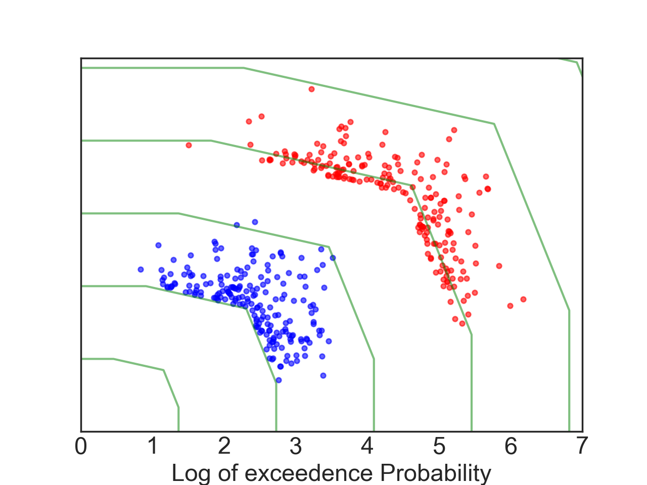
(a) Normal  marginals,$\,\rho=0.5$

(b) Weibull marginals,$\,\rho=0.3$

(c) Exponential marginals,$\,\rho=0.5$

To leverage this remarkable similarity in how the samples of $P_{u}^{\ast}$ and $P_{l}^{\ast}$ concentrate, we seek transformations which automatically replicate the large deviations concentration properties of $P_{u}^{\ast}$ from how the much more frequently occurring samples of $P_{l}^{\ast}$ manifest. As a product of this entirely novel approach, we are able to make the following main contributions in this paper.

1) Tail modeling framework characterizing self-similarity in optimal IS distributions: Building on the tail modeling approach introduced in de Valk, (2016), we identify a general class of models for which the above self-similarity in optimal IS distributions can be made precise in terms of large deviations principles (Proposition 4.1). This self-similarity phenomenon, being nonparametric in nature, is not limited to objectives/distributions fitting within specific parametric assumptions. As a result, our framework becomes the first to feature a rich set of models with

• objectives $L(\cdot)$ including, but not limited to, those specified in terms of tools such as linear programs, mixed-integer linear programs, piecewise linear and quadratic objectives, feature-maps/decision-rules informed by neural networks, etc., (see Assumption 2.1); and

• a wide variety of light and heavy-tailed multivariate distributions for $\boldsymbol{X}$ (see Assumptions 3.1, 3.2, 5.2 and the examples in Tables 2 - 4).

2) Novel approach to IS: We exhibit a fixed family of transformations (see (22)) which, despite being oblivious to the loss $L(\cdot)$ and the underlying distribution, is able to induce IS distributions with desirable properties in the considered generality: In particular, the target event $\{L(\boldsymbol{X})\geq u\}$ is shown to occur exponentially more frequently under the induced IS distributions, while also ensuring that the resulting conditional excess loss samples mirror the large deviations properties of the theoretically optimal $P_{u}^{\ast}.$ The need to explicitly formulate a good IS density family $\mathcal{P}$ and the optimization problem (OPT) (as described in Section 1.1) gets obviated with the radical discovery of these transformations, thereby rendering the selection of IS distributions entirely algorithmic.

3) An efficient IS algorithm with wider applicability: The use of the IS transformation in (22) results in a novel IS algorithm whose execution requires only oracle access to the evaluations of loss $L(\cdot)$ and the probability density of $\boldsymbol{X}$ (see Algorithm 1). We derive large deviations asymptotic for the distribution tails of $L(\boldsymbol{X})$ and show that the proposed sampler offers asymptotically optimal variance reduction in the considered generality (Theorems 4.1 - 5.3).

This is to be contrasted with the efficient IS changes of measures available, largely on a case-by-case basis, for specific highly stylized objectives $L(\cdot)$ and typically under normal distribution assumptions, i.i.d assumptions, or specific copula assumptions in the literature. The proposed sampler joins the recent line of enquiry initiated in the last couple of years (see Bai et al., 2022, Arief et al., 2021) striving to make IS amenable for more sophisticated objectives. The earlier works in this pursuit have restricted the focus to normal distributions and objectives which can be modeled or approximated by piecewise linear functions, with the complexity of the approach scaling less graciously in terms of the number of pieces involved. A distinguishing feature of the proposed sampler is that it is the first in the literature to consider a spectrum of multivariate light and heavy-tailed distributions simultaneously and achieve log-efficiency across this spectrum despite tackling several challenging and important objectives (such as value of linear programs, contextual optimization objectives, etc.) for which efficient IS algorithms are unavailable even under Gaussian distributional assumptions.

We demonstrate the utility of the IS scheme in the evaluation of probabilities of (a) large losses in a portfolio credit risk setting, and (b) large delays in contextual routing. The proposed sampler for portfolio credit risk also serves as an entirely novel addition that extends the scope of applicability of the line of research pursued in Glasserman et al., (2000), Glasserman & Li, (2005), Bassamboo et al., (2008), Glasserman et al., (2008), Liu, (2015) to credit risk models which employ diverse copula or algorithmic approaches such as neural networks. Following Glynn, (1996) and Hong et al., (2014), a follow-up to this work (Deo & Murthy, 2021) demonstrates how the IS scheme proposed in this paper for estimation of distribution tails can be employed to gain efficient variance reduction in Value-at-Risk and conditional Value-at-Risk estimation. Its use in further optimization tasks, such as minimizing conditional Value-at-Risk, is explored in Section G.

The rest of the paper is organized as follows. Following a description of the problem, our novel IS procedure is introduced in Section 2. The tail modeling framework introduced in Section 3 is used to establish the large deviations asymptotics and the self-similarity property of optimal IS distributions in Section 4. Section 5 identifies transformations capable of inducing efficient IS distributions and presents the main results verifying the asymptotic optimal variance reduction properties. An application to the portfolio credit risk setting and results of numerical experiments are presented in Sections 6 and 7. Proofs and additional useful examples are given in the accompanying supplementary material.

2. The problem considered and the proposed IS procedure

Vectors are written in boldface to enable differentiation from scalars. For any $\boldsymbol{a}=(a_{1},\ldots,a_{d})\in\mathbb{R}^{d},$ $\boldsymbol{b}=(b_{1},\ldots,b_{d})\in\mathbb{R}^{d}$ and $c\in\mathbb{R},$ we have $|\boldsymbol{a}|=(|a_{1}|,\ldots,|a_{d}|),$ $\boldsymbol{a}\boldsymbol{b}=(a_{1}b_{1},\ldots,a_{d}b_{d}),$ $\boldsymbol{a}/\boldsymbol{b}=(a_{1}/b_{1},\ldots,a_{d}/b_{d}),$ $\boldsymbol{a}\vee\boldsymbol{b}=(\max\{a_{1},b_{1}\},\ldots,\max\{a_{d},b_{d}\}),$ $\boldsymbol{a}^{\boldsymbol{b}}=(a_{1}^{b_{1}},\ldots,a_{d}^{b_{d}}),$ $\boldsymbol{a}^{-1}=(1/a_{1},\ldots,1/a_{d}),$ $\log\boldsymbol{a}=(\log a_{1},\ldots,\log a_{d}),$ $c^{\boldsymbol{a}}=(c^{a_{1}},\ldots,c^{a_{d}}),$ denoting the respective component-wise operations. Let $\mathbb{R}^{d}_{+}=\{\boldsymbol{x}\in\mathbb{R}^{d}:\boldsymbol{x}\geq\boldsymbol{0}\}$ denote the positive orthant and $\mathbb{R}^{d}_{++}$ denote its interior.

2.1. A description of the problem considered

Suppose that $L(\boldsymbol{x})$ denotes the cost incurred when the uncertain variables affecting the problem, modeled by a random vector $\boldsymbol{X},$ realize the value $\boldsymbol{x}\in\mathbb{R}^{d}.$ While the loss $L(\cdot)$ may be expressed as a linear combination of uncertain variables in some simple settings, the inherent nature of managing operations under resource constraints often results in $L(\cdot)$ expressed suitably as the value of an optimization formulation. We consider the task of estimating the probabilities or expectations associated with tail risk events of the form $\{L(\boldsymbol{X})\geq u\},$ for a threshold $u$ suitably large. The need for having a control over likelihoods of these risk scenarios is inherently present in many operational settings affected by uncertainty, due to the need to keep the costs below a target risk level (or) to meet a service-level agreement which ensures that a target quality of service is met. In many applications, high losses are experienced when the random vector $\boldsymbol{X}$ takes undesirably high values in the positive orthant; for example, large travel durations in vehicle routing instances leading to large delays. Thus, without loss of generality, we take the set specifying risk scenarios, $\{\boldsymbol{x}\in\text{supp}(\boldsymbol{X}):L(\boldsymbol{x})\geq u\},$ to be a subset of the positive orthant $\mathbb{R}^{d}_{+};$ here $\text{supp}(\boldsymbol{X})$ denotes the support of the distribution of $\boldsymbol{X}.$ Considering a rich class of loss functions $L(\cdot)$ satisfying Assumption 2.1 below, we aim to design efficient IS schemes for estimating the distribution tails of $L(\boldsymbol{X}).$

Assumption 2.1.

The function $L:\mathbb{R}^{d}\rightarrow\mathbb{R}$ satisfies the following conditions:

• the set $\{\boldsymbol{x}\in\textnormal{supp}(\boldsymbol{X}):L(\boldsymbol{x})\geq u\}$ is contained in $\mathbb{R}^{d}_{+}$ for all sufficiently large $u;$ and

• for any sequence $\{\boldsymbol{x}_{n}\}_{n\geq 1}$ of $\mathbb{R}^{d}_{+}$ satisfying $\boldsymbol{x}_{n}\rightarrow\boldsymbol{x},$ we have

  $$\lim_{n\rightarrow\infty}\frac{L(n\boldsymbol{x}_{n})}{n^{\rho}}=L^{\ast}(\boldsymbol{x}),$$

  where $\rho$ is a positive constant and the limiting function $L^{\ast}:\mathbb{R}^{d}_{+}\rightarrow\mathbb{R}$ is such that the cone $\{\boldsymbol{x}\in\mathbb{R}^{d}_{+}:L^{\ast}(\boldsymbol{x})>0\}$ is non-empty.

Assumption 2.1b merely specifies asymptotic homogeneity, which implies that larger the value of $u,$ farther is the target rare set from the origin. The set $\{\boldsymbol{x}\in\mathbb{R}^{d}_{+}:L^{\ast}(\boldsymbol{x})>0\}$ is necessarily a cone because $L^{\ast}(c\boldsymbol{x})=\lim_{n\rightarrow\infty}n^{-\rho}L(nc\boldsymbol{x})=c^{\rho}\lim_{n\rightarrow\infty}(cn)^{-\rho}L(cn\boldsymbol{x})=c^{\rho}L^{\ast}(\boldsymbol{x}),$ for any $c>0,\boldsymbol{x}\in\mathbb{R}^{d}_{+}.$ Examples 2.1 - 2.3 below provide a non-exhaustive yet indicative list of objectives $L(\cdot)$ for which Assumption 2.1 is readily satisfied. A discussion on verifying Assumption 2.1b when only oracle access to loss evaluations $L(\cdot)$ are available is presented in Section F. As Assumption 2.1 does not require convexity, the treatment in this paper is applicable even if $L(\cdot)$ is neither convex nor concave.

Example 2.1 (Piecewise affine functions, value of mixed integer linear programs).

Suppose that $L(\cdot)$ can be written as

$$L(\boldsymbol{x})=\sup_{\boldsymbol{\theta}\in\Theta}\{\boldsymbol{\theta}^{\intercal}\boldsymbol{x}+r(\boldsymbol{\theta})\},$$ (1)

where $\Theta$ is a bounded subset of $\mathbb{R}^{d}$ and $r:\Theta\rightarrow\mathbb{R}$ is a bounded function which serves to capture terms, if any, which do not involve the random vector $\boldsymbol{X}.$ In the case where $\Theta$ is a finite set, $L(\cdot)$ could represent a piecewise affine function as in, $L(\boldsymbol{x})=\max_{k=1,\ldots,K}\{\boldsymbol{\theta}_{k}^{\intercal}\boldsymbol{x}+r_{k}\},$ where $K$ is a positive integer, $\boldsymbol{\theta}_{k}\in\mathbb{R}^{d}$ and $r_{k}\in\mathbb{R},$ for $k=1,\ldots,K.$ If the set $\Theta$ is described by linear and/or integer constraints and if the function $r(\cdot)$ is affine, we have that (1) is a linear (or) a mixed integer linear program. With the notation used in Assumption 2.1, we have $\rho=1$ and $L^{\ast}(\boldsymbol{x})=\max_{\boldsymbol{\theta}\in\Theta}\boldsymbol{\theta}^{\intercal}\boldsymbol{x}$ for the example $L(\cdot)$ in (1); see (Rockafellar & Wets, 1998, Proposition 7.29). The requirements in Assumption 2.1 are met, for example, if at least one vector in the collection $\Theta$ lies outside the negative orthant $\mathbb{R}^{d}_{-};$ or, in other words, if $\sup\{\theta_{k}:(\theta_{1},\ldots,\theta_{d})\in\Theta,k=1,\ldots,d\}>0$. Objectives in many planning problems, such as project evaluation and review networks, linear assignment or matching, traveling salesman problem, vehicle routing problem, max-flow, minimum cost flow, etc., satisfy this requirement either in the native formulation or in the respective dual formulation. $\Box$

Example 2.2 (Piecewise quadratic functions).

As an extension to Example 2.1, one may also consider piecewise quadratic functions of the form $L(\boldsymbol{x})=\max_{k=1,\ldots,K}\left\{\boldsymbol{x}^{T}Q_{k}\boldsymbol{x}+\boldsymbol{c}_{k}^{T}\boldsymbol{x}\right\},$ where $K$ is a positive integer, $\{Q_{k}:k=1,\ldots,K\}$ are $(d\times d)$-symmetric matrices, and $\boldsymbol{c}_{k}\in\mathbb{R}^{d},$ for $k=1,\ldots,K.$ As long as the matrices $Q_{k}$ are not all identically zero, we have $\rho=2$ and $L^{\ast}(\boldsymbol{x})=\max\{\boldsymbol{x}^{T}Q_{k}\boldsymbol{x}:k=1,\ldots,K\}$ in this example. When the support of $\boldsymbol{X}$ is bounded from below, the requirements in Assumption 2.1 are automatically met if, for example, at least one of the eigen values of the matrices in the collection $\{Q_{k}:k=1,\ldots,K\}$ is positive. If $L(\cdot)$ is instead a piecewise-minimum as in $L(\boldsymbol{x})=\min_{k=1,\ldots,K}\left\{\boldsymbol{x}^{T}Q_{k}\boldsymbol{x}+\boldsymbol{c}_{k}^{T}\boldsymbol{x}\right\},$ the requirements are readily checked to be satisfied with $\rho=2$ if the collection $\{Q_{k}:k=1,\ldots,K\}$ is positive semidefinite. $\Box$

Example 2.3 (Models using contextual information via feature maps/decision rules).

Suppose that $L(\cdot)$ is written as a composition of functions as in $L(\boldsymbol{x})=c\left(\boldsymbol{\theta}^{\intercal}\boldsymbol{\Phi}(\boldsymbol{x})+\theta_{0}\right),$ where $c:\mathbb{R}\rightarrow\mathbb{R}$ is an objective measuring the cost incurred by plugging in a specific decision rule or a function approximation based on the feature map $\boldsymbol{\Phi}:\mathbb{R}^{d}\rightarrow\mathbb{R}^{m}$ (see Ban & Rudin, (2019) for an example use of feature-based decision rules in newsvendor models). In simple settings, one may take the feature map to be merely $\boldsymbol{\Phi}(\boldsymbol{x})=\boldsymbol{x},$ or, may include cross-terms in the feature vector as in $\boldsymbol{x}=(x_{1},\ldots,x_{d})\mapsto(x_{i},x_{i}x_{j}:i,j=1,\ldots,d).$ Motivated by the proliferation of deep neural networks in learning expressive feature maps, one may consider the feature map $\boldsymbol{\Phi}$ to be specified in terms of several function compositions defined recursively as in,

$$\boldsymbol{\Phi}(\boldsymbol{x})=\boldsymbol{L}_{K}(\boldsymbol{x}),\quad\boldsymbol{L}_{k}(\boldsymbol{x})=(A_{k}\boldsymbol{L}_{k-1}(\boldsymbol{x})-\boldsymbol{b}_{k})^{+},k=1,\ldots,K,\quad\text{ and }\quad L_{0}(\boldsymbol{x})=(A_{0}\boldsymbol{x}-\boldsymbol{b}_{0})^{+}.$$ (2)

In the above, the operation $(\boldsymbol{a})^{+}=\boldsymbol{a}\vee\boldsymbol{0},$ $K$ is a positive integer and for each $k\leq K,$ $A_{k}\in\mathbb{R}^{n_{k}\times n_{k-1}},$ $\boldsymbol{b}_{k}\in\mathbb{R}^{n_{k}}$ are weight parameters in a neural network with $n_{k}\geq 1$ rectified linear activation units (ReLU) in the $k$-th layer. We have $n_{K}=:m$ as the dimension of the resulting feature map. Refer Sadhwani et al., (2020) for a treatment of their utility in identifying relevant features in the context of modeling mortgage default risk. For the map $\boldsymbol{\Phi}(\cdot)$ considered in (2), we have

$$n^{-1}\boldsymbol{\Phi}(n\boldsymbol{x}_{n})\rightarrow\big{(}A_{K}\big{(}\cdots A_{1}(A_{0}\boldsymbol{x})^{+}\big{)}^{+}\big{)}^{+},\text{ for every sequence $\{\boldsymbol{x}_{n}\}_{n\geq 1}$ of $\mathbb{R}^{d}$ satisfying $\boldsymbol{x}_{n}\rightarrow\boldsymbol{x}.$ }$$

In general, suppose the feature map $\boldsymbol{\Phi}$ is such that $n^{-p}\boldsymbol{\Phi}(nx_{n})\rightarrow\boldsymbol{\Phi}^{\ast}(\boldsymbol{x}),$ for some $p>0$ and every sequence $\{\boldsymbol{x}_{n}\}_{n\geq 1}$ of $\mathbb{R}^{d}_{+}$ satisfying $\boldsymbol{x}_{n}\rightarrow\boldsymbol{x}.$ Then for the desired convergence in Assumption 2.1b, we have, $L^{\ast}(\boldsymbol{x})=c_{+}\big{[}\big{(}\boldsymbol{\theta}^{\intercal}\boldsymbol{\Phi}^{\ast}(\boldsymbol{x})\big{)}^{+}\big{]}^{q}\ +\ c_{-}\big{[}\big{(}\boldsymbol{\theta}^{\intercal}\boldsymbol{\Phi}^{\ast}(\boldsymbol{x})\big{)}^{-}\big{]}^{q}$ and $\rho=pq$, if, for example, $c(\cdot)$ is such that $c(u)/u^{q}\rightarrow c_{+}$ as $u\rightarrow\infty,$ $c(u)/|u|^{q}\rightarrow c_{-}$ as $u\rightarrow-\infty,$ with constants $q,c_{+},c_{-}$ satisfying $q>0,\min\{c_{+},c_{-}\}>0.$ One may include an additional composition to consider models of the form,

$$L(\boldsymbol{s},\boldsymbol{\varepsilon})=\min_{\boldsymbol{\theta}\in\boldsymbol{\Theta}}\ \boldsymbol{\theta}^{\intercal}\boldsymbol{c}\big{(}\boldsymbol{\Phi}(\boldsymbol{s}),\boldsymbol{\varepsilon}\big{)},$$ (3)

where $\boldsymbol{s}$ is seen as contextual side information, $\boldsymbol{\Phi}(\cdot)$ is a feature map that models the dependence of cost vector $\boldsymbol{c}$ in terms of the side information $\boldsymbol{s}$ and additional uncertainty $\boldsymbol{\varepsilon},$ and $\boldsymbol{\Theta}$ describes the constraints; see, for example, Elmachtoub & Grigas, (2022) for details and Section 7.1 for a contextual shortest-path example. Here suppose that the feature map $\boldsymbol{\Phi}(\cdot)$ is as above and the cost mapping $\boldsymbol{c}$ is positive and satisfies $n^{-\rho}\boldsymbol{c}(n^{p}\boldsymbol{s}_{n},n\boldsymbol{\varepsilon}_{n})\to\boldsymbol{c}^{\ast}(\boldsymbol{s},\boldsymbol{\varepsilon}),$ for $\boldsymbol{s}_{n}\rightarrow\boldsymbol{s},$ $\boldsymbol{\varepsilon}_{n}\to\boldsymbol{\varepsilon}$ and some $\rho,p>0.$ If we let $\boldsymbol{x}=(\boldsymbol{s},\boldsymbol{\varepsilon}),$ we have Assumption 2.1(b) satisfied with $L^{\ast}(\boldsymbol{s},\boldsymbol{\varepsilon})=\min_{\boldsymbol{\theta}\in\boldsymbol{\Theta}}\boldsymbol{\theta}^{\intercal}\boldsymbol{c}^{\ast}\big{(}\boldsymbol{\Phi}^{*}(\boldsymbol{s}),\boldsymbol{\varepsilon}\big{)}.$ $\Box$

One can identify more functionals $L(\cdot)$ which satisfy Assumption 2.1b) by taking linear combinations (that is, if $L_{1}$ and $L_{2}$ satisfy Assumption 2.1b), so does $L_{1}+L_{2}$) or compositions suitably (as in Example 2.3) based on modeling needs. Further, the requirements in Assumption 2.1b) can be recast naturally if a particular application requires the set quantifying risky scenarios, $\{\boldsymbol{x}:L(\boldsymbol{x})\geq u\},$ to be a subset in a different orthant.

2.2. The proposed importance sampling method

The proposed importance sampling (IS) procedure for fast evaluation of $p_{u}:=P(L(\boldsymbol{X})>u),$ where $L(\cdot)$ is taken to satisfy Assumption 2.1, is presented in Algorithm 1 below. A key ingredient of Algorithm 1 is a multiplicative transformation of the form,

$$\boldsymbol{T}(\boldsymbol{x})=\boldsymbol{x}\times\big{(}u/l\big{)}^{\boldsymbol{\kappa}(\boldsymbol{x})},$$ (4)

where $l\in[0,u]$ is a hyper-parameter choice and $\boldsymbol{\kappa}:\mathbb{R}^{d}\rightarrow\mathbb{R}^{d}_{+}$ is a suitably defined vector-valued map. One may view the components of $\boldsymbol{T}(\boldsymbol{x})=(T_{1}(\boldsymbol{x}),\ldots,T_{d}(\boldsymbol{x}))$ as a multiplicative stretching of the components of $\boldsymbol{x}=(x_{1},\ldots,x_{d})$ as in ${T}_{i}(\boldsymbol{x})=x_{i}\times(u/l)^{\kappa_{i}(\boldsymbol{x})}\geq x_{i},$ with the extent of stretch of each component determined by the respective exponent $\kappa_{i}(\boldsymbol{x})\geq 0.$

 

Input: Threshold $u,$ independent samples $\boldsymbol{X}_{1},\ldots,\boldsymbol{X}_{N}$ of $\boldsymbol{X},$ hyperparameter $l,$ specify if the exponent $\boldsymbol{\kappa}(\cdot)$ is chosen from (7) to be either $\boldsymbol{\kappa}=\boldsymbol{\kappa}^{(1)}$ (or) $\boldsymbol{\kappa}=\boldsymbol{\kappa}^{(2)}$

 

Procedure:

1. Transform the samples: For each sample $i=1,\ldots,N,$ compute the transformation,

$$\boldsymbol{Z}_{i}=\boldsymbol{T}(\boldsymbol{X}_{i}):=\boldsymbol{X}_{i}(u/l)^{\boldsymbol{\kappa}(\boldsymbol{X}_{i})},$$ (5)

 

2. Compute the associated likelihood: For each transformed sample $\boldsymbol{Z}_{i},$ compute the respective likelihood ratio as,

$$\mathcal{L}_{i}:=\frac{f_{\boldsymbol{X}}(\boldsymbol{Z}_{i})}{f_{\boldsymbol{X}}(\boldsymbol{X}_{i})}J(\boldsymbol{X}_{i}),\qquad i=1,\ldots,N,$$ (6)

where $f_{\boldsymbol{X}}(\cdot)$ is the probability density of $\boldsymbol{X}$ and $J:\mathbb{R}^{d}\rightarrow\mathbb{R}_{+}$ is the Jacobian of the transformation $T$ (see Table 1 for expressions of $J(\cdot)$ along with prescribed choices of $\boldsymbol{\kappa}(\cdot)$).

 

3. Return the output estimator: Return the IS average computed as in,

$$\bar{\zeta}_{{}_{N}}(u)=\frac{1}{N}\sum_{i=1}^{N}\mathcal{L}_{i}\mathbf{I}\left(L(\boldsymbol{Z}_{i})\geq u\right).$$

Algorithm 1 Self-structuring IS procedure for estimating $P(L(\boldsymbol{X})\geq u)$

We provide efficient variance reduction guarantees for Algorithm 1 when the transformation $\boldsymbol{T}(\cdot)$ is used in (5) with the exponent $\boldsymbol{\kappa}(\cdot)$ fixed to any one of the following two choices:

$$\boldsymbol{\kappa}^{(1)}(\boldsymbol{x}):=\frac{1}{\rho}\frac{\log(1+|\boldsymbol{x}|)}{\|\log(1+|\boldsymbol{x}|)\|_{\infty}},\qquad\boldsymbol{\kappa}^{(2)}(\boldsymbol{x}) :=\frac{\log(1+|\boldsymbol{x}|)}{\log l}.$$ (7)

While the former relies on knowledge of the growth parameter $\rho$ in Assumption 2.1, the latter is model-agnostic in the sense that it is free of any dependence on $L(\cdot)$ or the distribution of $\boldsymbol{X}.$ As a result, $\boldsymbol{\kappa}^{(2)}(\boldsymbol{x})$ is applicable more broadly in distribution tail estimation tasks including those in which evaluations of $L(\cdot)$ is available only via oracle queries. A discussion on how the choice $\boldsymbol{\kappa}^{(1)}(\boldsymbol{x})$ can be advantageous in preserving convexity of the objective if one is engaged in further optimization tasks (such as minimizing Conditional Value-at-Risk) is presented in Section G.

In Algorithm 1, the samples for the proposed IS procedure are taken as ${\boldsymbol{Z}}_{i}:=\boldsymbol{T}(\boldsymbol{X}_{i}),\quad i=1,\ldots,N,$ where $\boldsymbol{X}_{1},\ldots,\boldsymbol{X}_{N}$ are independent and identically distributed as $\boldsymbol{X}.$ The bias resulting from counting the fraction of samples $\boldsymbol{Z}_{i}$ lying in the target rare set, instead of that of $\boldsymbol{X}_{i},$ is adjusted by multiplying with the respective likelihood ratio term $\mathcal{L}_{i}$ as in,

$$\bar{\zeta}_{{}_{N}}(u)=\frac{1}{N}\sum_{i=1}^{N}\mathcal{L}_{i}\mathbf{I}\left(L(\boldsymbol{Z}_{i})\geq u\right),$$ (8)

to obtain the estimator $\bar{\zeta}_{{}_{N}}(u)$ returned by Algorithm 1. As with any IS procedure, the likelihood ratio term $\mathcal{L}_{i}$ is taken to be the ratio between the probability densities of $\boldsymbol{X}$ and $\boldsymbol{Z}$ evaluated at $\boldsymbol{Z}_{i}$ (see eg., Asmussen & Glynn, 2007, Chapter 5). With a standard change of variables formula involving the Jacobian of the transformation, $\mathcal{L}_{i}$ can be written conveniently as in Table 1 below. This involves plugging in the choice of $\boldsymbol{\kappa}$ in the Jacobian determinant

$$J(\boldsymbol{x}):=\text{det}\left(\frac{\partial\boldsymbol{T}(\boldsymbol{x})}{\partial\boldsymbol{x}}\right)=(u/l)^{\boldsymbol{1}^{\intercal}\boldsymbol{\kappa}(\boldsymbol{x})}\text{det}\left(\mathbb{I}_{d}+\ln\left(u/l\right)\text{Diag}(\boldsymbol{x})\frac{\partial\boldsymbol{\kappa}(\boldsymbol{x})}{\partial\boldsymbol{x}}\right),$$ (9)

almost everywhere, to obtain the associated likelihood ratio $\mathcal{L}_{i}=J(\boldsymbol{X}_{i})f_{\boldsymbol{X}}(\boldsymbol{Z}_{i})/f_{\boldsymbol{X}}(\boldsymbol{X}_{i}).$ Consequently, as verified in Proposition 2.1 below, the resulting estimator $\bar{\zeta}_{{}_{N}}(u)$ has no bias.

Table 1. Choice of the exponent $\boldsymbol{\kappa}(\cdot)$ in (4) and the respective Jacobian determinant

Choice of exponent $\boldsymbol{\kappa}$ in	Jacobian determinant $J(\boldsymbol{X}_{i})$ in the respective	Additional remarks
$\boldsymbol{T}(\boldsymbol{X}_{i})=\boldsymbol{X}_{i}\left(u/l\right)^{\boldsymbol{\kappa}(\boldsymbol{X}_{i})}$	likelihood ratio $\mathcal{L}_{i}=J(\boldsymbol{X}_{i})\frac{f_{\boldsymbol{X}}(Z_{i})}{f_{\boldsymbol{X}}(X_{i})}$
$\boldsymbol{\kappa(\boldsymbol{x})}=\boldsymbol{\kappa^{(1)}(\boldsymbol{x})}$	$J(\boldsymbol{x})=\left[\prod_{k=1}^{d}\tilde{J}_{k}(\boldsymbol{x})\right]\times\frac{(u/l)^{\boldsymbol{1}^{\intercal}\boldsymbol{\kappa}(\boldsymbol{x})}}{\max_{k=1,\ldots,d}\tilde{J}_{k}(\boldsymbol{x})},$	$\circ$ Relies on knowing $\rho$
	where	$\circ$ Advantageous in
	$\quad\tilde{J}_{k}(\boldsymbol{x}):=1+\frac{\rho^{-1}\log(u/l)}{\|\log(1+|\boldsymbol{x}|)\|_{\infty}}\frac{|x_{k}|}{1+|x_{k}|},\ \ k=1,\ldots,d$	retaining convexity
		in optimization tasks
$\boldsymbol{\kappa(\boldsymbol{x})}=\boldsymbol{\kappa^{(2)}(\boldsymbol{x})}$	$J(\boldsymbol{x})=\left[\prod_{i=1}^{d}\bar{J}_{k}(\boldsymbol{x})\right]\times(u/l)^{\boldsymbol{1}^{\intercal}\boldsymbol{\kappa}(\boldsymbol{x})}$	$\circ\$resulting $\boldsymbol{T}$ in (4)
	where	does not depend on
	$\quad\bar{J}_{k}(\boldsymbol{x})=1+\frac{\log(u/l)}{\log l}\frac{|x_{k}|}{1+|x_{k}|},\quad k=1,\ldots,d$	$L(\cdot)$ or pdf of $\boldsymbol{X}$

Proposition 2.1.

Suppose that the transformation $\boldsymbol{T}$ in (5) is employed with either $\boldsymbol{\kappa}(\boldsymbol{X}_{i})=\boldsymbol{\kappa}^{(1)}(\boldsymbol{X}_{i})$ (or) $\boldsymbol{\kappa}(\boldsymbol{X}_{i})=\boldsymbol{\kappa}^{(2)}(\boldsymbol{X}_{i}),$ and the likelihood ratio $\mathcal{L}_{i}$ in (6) is computed with the respective Jacobian determinant in Table 1. Then for any $u>0,$ the estimator $\bar{\zeta}_{{}_{N}}(u)$ is unbiased. In other words, $E[\bar{\zeta}_{{}_{N}}(u)]=p_{u}.$ Moreover there exists a map $\boldsymbol{T}^{-1}:\mathbb{R}^{d}\rightarrow\mathbb{R}^{d}$ such that $\boldsymbol{T}\circ\boldsymbol{T}^{-1}(\boldsymbol{x})=\boldsymbol{x}$ for almost every $\boldsymbol{x}\in\mathbb{R}^{d}.$

The choice of the transformation $\boldsymbol{T}(\cdot)$ in Algorithm 1, which implicitly specifies the IS density, is guided by the self-similarity properties of the distribution of $\boldsymbol{X}$ to be made concrete with the large deviations framework in following Sections 3 - 4. Building on this framework, an account on the rationale behind the choice of the IS transformation $\boldsymbol{T}$ and its variance reduction properties is offered in Section 5. Roughly speaking, the transformation $\boldsymbol{T}(\cdot)$ seeks to suitably replicate the concentration properties of the theoretically optimal IS distribution from observations which are not as rare. This is facilitated by taking the parameter $l$ such that $l\ll u$ and the event $\{L(\boldsymbol{X})\geq l\},$ though also a tail risk event, is much more frequently observed in the initial samples when compared to the target event $\{L(\boldsymbol{X})\geq u\}.$ Even if the parameter $l$ is relatively negligible when compared to the level $u,$ we show the variance of the resulting IS estimator is small as in,

$$\text{var}[\,\bar{\zeta}_{{}_{N}}(u)\,]=o\left(p_{u}^{2-\varepsilon}N^{-1}\right),$$ (10)

as the estimation task is made more challenging by taking $p_{u}\rightarrow 0.$ The relationship (10) holds for any arbitrary $\varepsilon>0$ and any choice of $l=l(u)$ which is taken to be slowly varying in $u$ and satisfying $\lim_{u\rightarrow\infty}l(u)=+\infty;$ see Theorem 5.1 in Section 5 for a precise statement of the variance reduction result and Section 3.1 for the definition and examples of slowly varying functions.

Recall from Section 1.1 that traditional IS approaches typically require solving a non-trivial optimization problem (OPT) to identify the best distribution within a chosen family IS distribution $\mathcal{P}.$ Unlike these procedures, the selection of IS density in our approach is simplified to that of selecting the single parameter $l$ minimizing the sample variance. The robust variance reduction guarantee for Algorithm 1, obtained for any $l$ which is slowly varying in $u,$ enables to confine the search for a good choice of the hyper-parameter $l$ to be within a relatively narrow collection. One may execute the selection of $l$ by means of cross-validation over candidate choices of $l,$ (or) with a retrospective approximation based search procedure we provide in Section 7 together with numerical examples.

Contrast the reduced variance of the IS estimator in (10) with that of the naive sample average which merely counts the fraction of samples $\{\boldsymbol{X}_{i}:i=1,\ldots,N\}$ in the target rare set. In the case of naive sample average, the variance is $p_{u}(1-p_{u})N^{-1}$ and the coefficient of variation grows as in $p_{u}^{-1}N^{-1/2},$ as $p_{u}\rightarrow 0.$ Thanks to (10), the coefficient of variation of the proposed IS estimator grows only as $o(p_{u}^{-\varepsilon}N^{-1/2})$ where $\varepsilon$ can be arbitrarily small, thus requiring only a negligible fraction of samples compared to that required by the naive sample average. Any estimator which meets the relative error guarantee in (10) is said to offer asymptotically optimal variance reduction and is referred to as logarithmically efficient. Please refer Asmussen & Glynn, (2007, Chapter 6) for a discussion on the significance on logarithmic efficiency and why it is a natural and pragmatic efficiency criterion for estimation tasks pertaining to rare events.

3. A nonparametric tail modeling description and associated LDP

3.1. Preliminaries: Regularly varying functions (Class $\boldsymbol{\mathscr{RV}}$)

A function $f:\mathbb{R}_{+}\rightarrow\mathbb{R}_{+}$ is said to be regularly varying with index $\rho\in\mathbb{R}$ if for every $x>0,$

$$\lim_{n\rightarrow\infty}\frac{f(nx)}{f(n)}=x^{\rho}.$$ (11)

When referring to (11), we write $f\in\mathscr{RV},$ or, $f\in\mathscr{RV}(\rho)$ if there is a need to explicitly specify the exponent $\rho$. The function $f(x)=x^{\rho}$ is a canonical example of the class $\mathscr{RV}(\rho).$ If $\rho=0,$ then $f$ is specifically referred as slowly varying. Some examples of slowly varying functions include $\log(1+x),$ $\log\log(e+x),(1+\log(1+x))^{a}$ where $a\in\mathbb{R},$ $\exp(\log(x)^{a})$ where $a\in(0,1),$ or any function $f$ satisfying $\lim_{x\rightarrow\infty}f(x)=c\in(0,\infty).$ A function $f\in\mathscr{RV}(\rho)$ can be written as $f(x)=\ell(x)x^{\rho},$ for some slowly varying $\ell(\cdot)$ and $\rho\in\mathbb{R}.$ Evidently, (11) is a characteristic of all homogeneous functions and univariate polynomials. By allowing $\rho$ to be an arbitrary real number and $\ell(\cdot)$ to be any slowly varying function, the class $\mathscr{RV}$ possesses substantially improved modeling power. See, for example, Borovkov, (2008) for a detailed treatment of the properties of the class $\mathscr{RV}.$

3.2. Assumptions on the probability distribution of $\boldsymbol{X}$

Let $\bar{F}_{i}(x_{i}):=P(X_{i}>x_{i})$ and $\Lambda_{i}(x_{i}):=-\log\bar{F}_{i}(x_{i})$ respectively denote the complementary c.d.f (also known as survival function) and the cumulative hazard function of the component $X_{i}$ in $\boldsymbol{X}=(X_{1},\ldots,X_{d}).$ The marginal components $X_{i}$ are required to satisfy Assumption 3.1 below.

Assumption 3.1.

For $i\in\{1,\ldots,d\},$ the marginal components $X_{i}$ are such that $\Lambda_{i}$ is continuous, strictly increasing in an interval of the form $(x_{0},\infty),$ and $\Lambda_{i}\in\mathscr{RV}(\alpha_{i})$ for some $\alpha_{i}\in(0,\infty).$

Common examples of distributions which satisfy Assumption 3.1 are as follows: standard exponential distribution where $\Lambda_{i}(x)=x$ satisfies $\Lambda_{i}\in\mathscr{RV}(1);$ standard normal distribution where $\Lambda_{i}(x)=x^{2}/2-\log x(1+o(1)),$ as $x\rightarrow\infty,$ satisfies $\Lambda_{i}\in\mathscr{RV}(2);$ Weibull distribution with shape parameter $k\in(0,\infty),$ where $\Lambda_{i}(x)=x^{k},$ satisfies $\Lambda_{i}\in\mathscr{RV}(k).$ Other examples of parametric families, along with respective tail parameters $\alpha_{i},$ are given in Table 2 in Appendix B. This large class includes distributions which are light-tailed and as well as heavy-tailed distributions of the Weibull type. The case where the marginal distributions possess even heavier tails, such as log-normal, pareto, regularly varying distributions, etc., are treated later in Section 5.3.

To describe the joint distribution of $\boldsymbol{X}$, we first consider the standardizing transformation,

$$\boldsymbol{Y}=(Y_{1},\ldots,Y_{d}):=\boldsymbol{\Lambda}(\boldsymbol{X}),\qquad\text{ where }\boldsymbol{\Lambda}(\boldsymbol{x}):=(\Lambda_{1}(x_{1}),\ldots,\Lambda_{d}(x_{d})),$$

which “standardize” the marginal distributions to that of standard exponential.

Lemma 3.1.

The marginal distributions of the components $Y_{i},$ for $i=1,\ldots,d,$ are identical and is given by, $P(Y_{i}>y_{i})=\exp\left(-y_{i}\right),$ for $y_{i}>0.$

As with the wide-spread practice of modeling joint distributions in terms of copulas (eg., Embrechts et al., 2001), this standardization restricts the focus to the dependence structure without getting distracted by the potential non-identical nature of marginal distributions of $\boldsymbol{X}.$

Assumption 3.2.

The probability density of $\boldsymbol{Y}:=\boldsymbol{\Lambda}(\boldsymbol{X})$ admits the form

$$f_{\boldsymbol{Y}}(\boldsymbol{y})=p(\boldsymbol{y})\exp(-\varphi(\boldsymbol{y})),$$ (12)

where $\varphi(\cdot),p(\cdot)$ satisfy the following: There exists a limiting function $I:\mathbb{R}^{d}_{+}\rightarrow\mathbb{R}_{+}$ such that,

$$n^{-1}\varphi(n\boldsymbol{y}_{n})\rightarrow I(\boldsymbol{y})\quad\text{ and }\quad n^{-\varepsilon}\log p(n\boldsymbol{y}_{n})\rightarrow 0,$$ (13)

for any sequence $\{\boldsymbol{y}_{n}\}_{n\geq 1}$ of $\mathbb{R}^{d}_{+}$ satisfying $\boldsymbol{y}_{n}\rightarrow\boldsymbol{y}\neq\boldsymbol{0},$ and $\varepsilon>0.$

A sufficient condition for $\boldsymbol{X}$ to satisfy Assumption 3.2 is that its pdf is of the form $f_{\boldsymbol{X}}(\boldsymbol{x})=\exp(-\psi(\boldsymbol{x})),$ where $\psi$ is multivariate regularly varying (see Section B for a definition of multivariate regularly varying functions and a precise statement of the sufficient condition). The nonparametric nature of the assumption suggests that a wide variety of dependence models satisfy Assumption 3.2. Indeed, most commonly used distribution families such as multivariate normal, multivariate $t$, elliptical densities, archimedean copula models, exponential family with any regularly varying sufficient statistic, extreme value distributions, suitable members of generalized linear models, log-concave densities, etc. can be verified to satisfy Assumption 3.2. Table 4 in Appendix B is intended to offer a sample of distribution families which satisfy the marginal and joint distribution conditions in Assumption 3.1 - 3.2 and to serve as a quick reference for the limiting function $I(\cdot)$ in Assumption 3.2.

Example 3.1 (Gaussian copula).

Suppose that $\boldsymbol{Y}$ has a joint distribution given by a Gaussian copula with correlation matrix $R.$ Given a copula with density $c:[0,1]^{d}\rightarrow[0,1],$ the respective probability density $f_{\boldsymbol{Y}}(\cdot)$ can be expressly computed as, $f_{\boldsymbol{Y}}(\boldsymbol{y})=c\big{(}\boldsymbol{1}-\exp(-\boldsymbol{y})\big{)}\exp(-\boldsymbol{1}^{\intercal}\boldsymbol{y})$. Therefore

$$f_{\boldsymbol{Y}}(\boldsymbol{y})=[\textnormal{det}({R})]^{-1/2}\exp\left(-\boldsymbol{1}^{\intercal}\boldsymbol{y}-2^{-1}\boldsymbol{g}(\boldsymbol{y})^{\intercal}(R^{-1}-\mathbf{I})\boldsymbol{g}(\boldsymbol{y})\right),$$

where $\boldsymbol{g}(\boldsymbol{y}):=(\bar{\Phi}^{-1}(\mathrm{e}^{-y_{1}}),\ldots,\bar{\Phi}^{-1}(\mathrm{e}^{-y_{d}}))$ and $\bar{\Phi}(\cdot):=1-\Phi(\cdot)$ is the complementary c.d.f. of the standard normal variable. Thus, in this example, we have from the notation in (12) that $p(\boldsymbol{y})=[\textnormal{det}({R})]^{-1/2}$ and $\varphi(\boldsymbol{y})=-\boldsymbol{1}^{\intercal}\boldsymbol{y}-2^{-1}\boldsymbol{g}(\boldsymbol{y})^{\intercal}(R^{-1}-\mathbf{I})\boldsymbol{g}(\boldsymbol{y}).$ Since $\bar{\Phi}^{-1}(p)=-2\log p\ (1+o(1)),$ as $p\rightarrow 0,$ we have $\boldsymbol{g}(n\boldsymbol{y})/(n)\rightarrow(y_{1}^{1/2},\ldots,y_{d}^{1/2}),$ and subsequently, $\varphi(n\boldsymbol{y})/\varphi(n)\rightarrow(\boldsymbol{y}^{1/2})^{\intercal}R^{-1}\boldsymbol{y}^{1/2},$ compactly, as $n\rightarrow\infty.$ We therefore have the limiting $I(\cdot)$ in Assumption 3.2 as $I(\boldsymbol{y}):=(\boldsymbol{y}^{1/2})^{\intercal}R^{-1}\boldsymbol{y}^{1/2}.$ $\Box$

Properties of the limiting function $I(\cdot)$ and a continued account of the distributions satisfying Assumption 3.2 are presented after introducing the tail large deviations principle in Section 3.3.

3.3. Tail large deviations principle with $I(\cdot)$ as the rate function

A sequence of random vectors $\boldsymbol{\xi}_{n}$ is said to satisfy a Large Deviations Principle (LDP) with rate function $J(\cdot)$ and speed $r_{n}\rightarrow\infty$ if,

$$\limsup_{n\rightarrow\infty}\frac{1}{r_{n}}\log P\left(\boldsymbol{\xi}_{n}\in F\right)\leq-\inf_{\boldsymbol{x}\in F}J(\boldsymbol{x})\quad\text{ and }\quad\liminf_{n\rightarrow\infty}\frac{1}{r_{n}}\log P\left(\boldsymbol{\xi}_{n}\in G\right)\geq-\inf_{\boldsymbol{x}\in G}J(\boldsymbol{x}),$$

for every closed subset $F$ and open subset $G.$ Theorem 3.1 below establishes the LDP which is useful in the context considered.

Theorem 3.1 (Tail LDP).

Suppose that $\boldsymbol{Y}$ is a random vector whose probability density admits the form (12), where the functions $\varphi(\cdot),p(\cdot)$ satisfy the convergences in (13) for any sequence $\{\boldsymbol{y}_{n}\}_{n\geq 1}$ of $\mathbb{R}^{d}_{+}$ satisfying $\boldsymbol{y}_{n}\rightarrow\boldsymbol{y}\neq\boldsymbol{0},$ and $\varepsilon>0.$ Then the sequence $\{n^{-1}\boldsymbol{Y}:n\geq 1\}$ satisfies the large deviations principle with rate function $I(\cdot)$ and speed $n$.

The following useful properties of the limiting function $I:\mathbb{R}^{d}_{+}\rightarrow\mathbb{R}$ in (13) are deduced from the conditions in Assumption 3.2 and the conclusion in Theorem 3.1.

Lemma 3.2.

Suppose that Assumption 3.2 holds. Then

• $I(\cdot)$ is continuous, $I(\boldsymbol{0})=0$ and $I(\boldsymbol{x})>0$ for all $\boldsymbol{x}\in\mathbb{R}_{d}^{+}\setminus\{\boldsymbol{0}\};$

• $I(\cdot)$ is homogeneous: that is, $I(\lambda\boldsymbol{x})=\lambda I(\boldsymbol{x}),$ for any $\lambda>0,\boldsymbol{x}\in\mathbb{R}_{d}^{+};$

• $I(\cdot)$ has compact level sets; specifically, $\inf_{\boldsymbol{x}\in\mathbb{R}^{d}_{+}:x_{i}>c}I(\boldsymbol{x})=c,$ for all $c\geq 0$ and $i=1,\ldots,d.$

Conversely, any function $I:\mathbb{R}^{d}_{+}\rightarrow\mathbb{R}_{+}$ which satisfies the above conditions can be used to readily specify a joint distribution for $\boldsymbol{Y}$ which has standard exponential marginals and satisfies the tail LDP. This is verified, for instance, by considering $\boldsymbol{Y}$ for which $P(\boldsymbol{Y}>\boldsymbol{y})=\exp(-\inf_{\boldsymbol{z}>\boldsymbol{y}}I(\boldsymbol{z})).$

Figure 2. Illustration of the level sets of $I(\cdot)$ capturing different strengths of the positive (indicated (+)) or negative (indicated (-)) tail correlations between the components of $\boldsymbol{Y}=(Y_{1},Y_{2}).$ Range of axes =[0,5]

(a) Gaussian copula(+)

(b) Gaussian copula (-)

(c) Clayton copula (+)

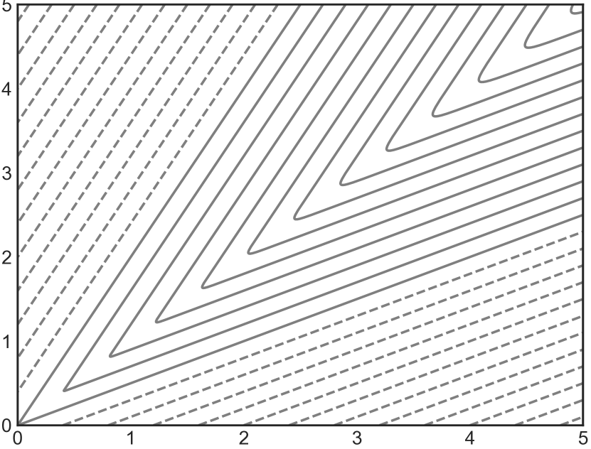
(d) Clayton copula (-)

While the rate function $I(\cdot)$ is unique for a given distribution for which the tail LDP holds, it is instructive to note that there may be multiple distributions which give rise to the same limit $I(\cdot).$ Indeed, the relation “has the same rate function $I(\cdot)$ in the tail LDP” is an equivalence relation, and every function $I(\cdot)$ satisfying properties (a) - (c) in Lemma 3.2 specifies a equivalence class of distributions for the random vector $\boldsymbol{Y}.$ Thus, the nonparametric nature of the limiting function $I(\cdot)$ offers a great amount of expressive power in capturing the joint dependence features observed in the the tail regions. The hazard functions $\Lambda_{1}(\cdot),\ldots,\Lambda_{d}(\cdot)$ in Assumption 3.1, on the other hand, offer flexibility in terms of specifying marginal distributions with various tail strengths.

4. Large deviations characterizations and zero-variance IS distributions

We begin by characterizing the exponential rate at which $P(L(\boldsymbol{X})\geq u)$ decays as in,

$$P(L(\boldsymbol{X})\geq u)=\exp\{-t(u)[I^{\ast}+o(1)]\},\quad\text{ as }u\rightarrow\infty,$$

where the function $t(u),$ which grows to infinity as $u\rightarrow\infty,$ is identified in terms of the marginal hazard functions $\Lambda_{1},\ldots,\Lambda_{d}$ described in Assumption 3.1, and the constant $I^{\ast}$ is identified in terms of the marginal tail parameters $\boldsymbol{\alpha}=(\alpha_{1},\ldots,\alpha_{d})$ and the limiting functions $L^{\ast}(\cdot)$ and $I(\cdot)$ in Assumptions 2.1 and 3.2. In order to state the result, let us define $\Lambda_{\min}:\mathbb{R}_{+}\rightarrow\mathbb{R}_{+}$ and $\hat{\boldsymbol{q}}:\mathbb{R}_{+}\rightarrow\mathbb{R}^{d}_{+}$ as,

$$\Lambda_{\min}(u):=\min_{i=1,\ldots,d}\Lambda_{i}(u)\quad\text{ and }\quad\hat{\boldsymbol{q}}(t):=\frac{\boldsymbol{q}(t\boldsymbol{1})}{\ \ \|\boldsymbol{q}(t\boldsymbol{1})\|_{\infty}},$$ (14)

where $\boldsymbol{q}:\mathbb{R}_{+}^{d}\rightarrow\mathbb{R}^{d}$ denotes the component-wise inverse $\boldsymbol{q}(\boldsymbol{y})=(q_{1}(y_{1}),\ldots,q_{d}(y_{d})),$ with $q_{i}(y_{i})={\Lambda}_{i}^{\leftarrow}(y_{i})$ specifying the left-continuous inverse of the hazard function $\Lambda_{i}(\cdot).$

Theorem 4.1 (Tail asymptotic).

Suppose that the marginal distributions of the components $X_{1},\ldots,X_{d}$ of the random vector $\boldsymbol{X}=(X_{1},\ldots,X_{d})$ satisfy Assumption 3.1 and the standardized vector $\boldsymbol{Y}=\boldsymbol{\Lambda}(\boldsymbol{X})$ is such that the tail LDP in Theorem 3.1 holds. Further suppose that the limit $\boldsymbol{q}^{\ast}:=\lim_{t\rightarrow\infty}\hat{\boldsymbol{q}}(t)$ exists. Then, for any $L(\cdot)$ satisfying Assumption 2.1,

$${\log P\left(L(\boldsymbol{X})\geq u\right)}=-{\Lambda_{\min}\big{(}u^{1/\rho}\big{)}}\big{[}I^{\ast}+o(1)\big{]},$$ (15)

as $u\rightarrow\infty;$ here the non-negative constant $I^{\ast}$ is given by,

$$I^{\ast}:=\inf\big{\{}I(\boldsymbol{y}):L^{\ast}\big{(}\boldsymbol{q}^{\ast}\boldsymbol{y}^{\boldsymbol{1}/\boldsymbol{\alpha}}\big{)}\geq 1,\ \boldsymbol{y}\geq\boldsymbol{0}\big{\}}.$$ (16)

As a consequence of Theorem 3.1, the tail asymptotic in (15) holds automatically for any joint distribution specified via Assumptions 3.1 - 3.2. While there is a rich literature on tail risk probabilities of the form $P(X_{1}+\cdots+X_{d}\geq u)$ where $X_{1},\ldots,X_{d}$ are independent, the treatment for more general objectives which arise in modeling operations exist only for specific instances. As examples, we have Glasserman et al., (2000) deriving asymptotics of the form (15) for a specific quadratic objective $L(\cdot)$ motivated from the delta-gamma approximation of portfolio losses. Likewise, Juneja et al., (2007), Blanchet et al., (2019), Ahn & Kim, (2018), Bai et al., (2022) derive asymptotics of the form (15) considering piecewise linear $L(\cdot)$ motivated from settings requiring evaluation of the likelihood of excessive project delays, cascading failures in product distribution and banking networks, safety in intelligent physical systems, etc. These results rely, however, on exploiting the specific structure of $L(\cdot)$ and the distributional assumptions such as $\boldsymbol{X}$ being multivariate normal, or elliptical, or possessing independent components. On the other hand, Theorem 4.1 is applicable for $L(\cdot)$ as general as the instances considered in Examples 1-2.3 and across a broad spectrum of distributions.

Remark 4.1 (Sufficient conditions on existence of $\boldsymbol{q}^{\ast}$).

Let $r_{i}(x):=\Lambda_{\min}(x)/\Lambda_{i}(x),$ $i=1,\ldots,d,$ and $\alpha_{\ast}:=\min_{i=1,\ldots,d}\alpha_{i}.$ With $\boldsymbol{q}:=\boldsymbol{\Lambda}^{\leftarrow},$ the limit $\boldsymbol{q}^{\ast}=(q^{\ast}_{1},\ldots,q_{d}^{\ast}),$ when exists, satisfies,

$${q}^{\ast}_{i}=\lim_{x\rightarrow\infty}r_{i}(x)^{1/\alpha_{\ast}},$$ (17)

for $i$ in $\{1,\ldots,d\};$ see the discussion at the end of Appendix D for additional explanation. Then for any $i$ such that $\alpha_{i}>\alpha_{\ast},$ the limit in (17) expressly evaluates to ${q}_{i}^{\ast}=0.$ For all $i$ such that $\alpha_{i}=\alpha_{\ast},$ we have that the limit in (17) exists if $\Lambda_{i}(x)=x^{\alpha_{\ast}}(c_{i}+o(1)),$ for some positive constant $c_{i};$ or more generally if $|\frac{d}{dx}r_{i}(x)|=O(x^{-(1+\varepsilon)}),$ for some $\varepsilon>0.$ As the latter condition merely restricts the magnitude of oscillations of the ratio $\Lambda_{\min}(x)/\Lambda_{i}(x),$ we have that the limit $\boldsymbol{q}^{\ast}$ exists for commonly used parametric distribution families.

To interpret the tail asymptotic (15), first note that the occurrence of $\Lambda_{\min}(\cdot):=\min_{i=1,\ldots,d}\Lambda_{i}(\cdot)$ in the denominator in (15) is aligned with the phenomenon that the “heaviest tail wins”. This observation is well-known within the specialized context of sums of random variables (see, for eg., Hult et al., 2012, Example 8.17). Thus, as is expected, the presence of an heavier tail results in larger probability for $P(L(\boldsymbol{X})\geq u).$ With $\boldsymbol{q}^{\ast}$ characterized as in (17) in terms of the ratio $r_{i}(x):=\Lambda_{\min}(x)/\Lambda_{i}(x),$ the appearance of $\boldsymbol{q}^{\ast}$ in (15) captures the differences in tail heaviness of the marginal distributions of $X_{1},\ldots,X_{d}.$ In the simpler case where all the components are identically distributed, we have $\boldsymbol{q}^{\ast}=1.$ If, for example, $X_{1}$ is the component with the heaviest tail in $\boldsymbol{X}=(X_{1},X_{2})$ and if $P(X_{1}>x)/P(X_{2}>x)=O(1)$ as $x\rightarrow\infty,$ then $\boldsymbol{q}^{\ast}=(1,c)$ for some constant $c\in(0,1);$ if on the other hand, $\Lambda_{1}(x)/\Lambda_{2}(x)\rightarrow\infty,$ then $\boldsymbol{q}^{\ast}=(1,0).$ The same description is applicable in higher dimensions where $d>2.$

Recall from Section 1.1 that the theoretically optimal IS distribution, which possesses zero variance in the estimation of $P(L(\boldsymbol{X})\geq u),$ is merely the conditional distribution

$$P_{u}^{\ast}(d\boldsymbol{x})\ :=\ P\left(\boldsymbol{X}\in d\boldsymbol{x}\,|\,L(\boldsymbol{X})\geq u\right)=\frac{f_{\boldsymbol{X}}(\boldsymbol{x})}{P(L(\boldsymbol{X})\geq u)}d\boldsymbol{x}.$$ (18)

For brevity, let $\boldsymbol{Z}_{u}^{\ast}$ be such that the $\text{law of }\boldsymbol{Z}_{u}^{\ast}=P_{u}^{\ast}$ for $u>0.$ Proposition 4.1 below gives an LDP for the collection $\{\boldsymbol{Z}_{u}^{\ast}:u>0\}.$ For $l<u,$ the LDP reveals how a suitably scaled version of $\boldsymbol{Z}_{l}^{\ast}\sim P_{l}^{\ast}$ can be seen to concentrate in regions similar to that of $\boldsymbol{Z}_{u}^{\ast}.$ In what follows, let $I^{\ast}$ be as defined in (16) and functions $\chi_{1}:\mathbb{R}^{d}\rightarrow\{0,+\infty\},$ $t:\mathbb{R}_{+}\rightarrow\mathbb{R}_{+}$ be defined as below:

$$\chi_{1}(\boldsymbol{y}):=\begin{cases}0,\quad&\text{ if }L^{*}(\boldsymbol{q}^{*}\boldsymbol{y}^{1/\boldsymbol{\alpha}})\geq 1,\\ +\infty,&\text{ otherwise},\end{cases}\quad\text{ and }\quad t(v):=\Lambda_{\min}(v^{1/\rho}).$$

Proposition 4.1 (Self-similarity in zero variance distributions).

Under the assumptions in Theorem 4.1, the collection $\{\boldsymbol{\Lambda}(\boldsymbol{Z}_{u}^{\ast})/t(u)\}_{u>0}$ satisfies LDP with rate function $I^{\prime}(\cdot)=I(\cdot)-I^{\ast}+\chi_{1}(\cdot)$ and speed $t(u),$ as $u\rightarrow\infty.$ Further, if $l$ is such that $l\to\infty$ and $u/l\to s\in(1,\infty]$ as $u\rightarrow\infty,$ then

$$P\left(\boldsymbol{Z}_{u}^{\ast}/\boldsymbol{q}(t(u))\in A\right) =\exp\left(-t(u)\left[I^{\prime}(A)+o(1)\right]\right),\quad\text{ and }$$

$$P\left(\boldsymbol{Z}_{l}^{\ast}/\boldsymbol{q}(t(l))\in A\right) =\exp\left(-t(l)\left[I^{\prime}(A)+o(1)\right]\right),$$

where $A$ is any closed subset of $\mathbb{R}^{d}$ and the respective $I^{\prime}(A):=\inf_{\boldsymbol{p}\in A}I^{\prime}(\boldsymbol{p}^{\boldsymbol{\alpha}})$.

5. Variance reduction properties of Algorithm 1

Building on the large deviations characterizations in Sections 3 - 4, this section aims to (i) bring out the rationale behind the choice of $\boldsymbol{T}(\cdot)$ employed in Algorithm 1; and (ii) establish the optimal variance reduction properties of the IS estimator $\bar{\zeta}_{{}_{N}}(u)$ returned by Algorithm 1.

5.1. Deducing effective IS transformations from large deviations

The zero variance distribution in (18) is not practical as a choice of IS distribution as its specification relies on the unknown quantity $P(L(\boldsymbol{X})\geq u).$ Despite this limitation, the zero-variance distribution is often utilized as a guide for identifying a good choice of IS distribution. Indeed, most verifiably effective IS schemes seek to identify a proposal IS distribution which possess relevant aspects of the respective zero-variance IS distribution and approximate it in a suitable manner (see, for eg., Juneja & Shahabuddin, 2002, Asmussen & Glynn, 2007, Chapter 6). In Definition 5.1 below, we instead seek transformations $\{\boldsymbol{T}_{u}:u>0\}$ such that (i) the distribution of $\boldsymbol{T}_{u}(\boldsymbol{X})\mid L(\boldsymbol{T}_{u}(\boldsymbol{X}))\geq u$ and the zero-variance distribution $P_{u}^{\ast}$ in (18) share similar large deviation properties; and (ii) the risky scenarios in the target rare set $\{\boldsymbol{x}:L(\boldsymbol{x})\geq u\}$ occur exponentially more frequently under the distribution of $\boldsymbol{T}_{u}(\boldsymbol{X}).$ Throughout this section, let $\boldsymbol{T}_{u}$ denote a mapping with domain and co-domain to be $\mathbb{R}^{d}$ and $\boldsymbol{Z}_{u}$ denote the conditional realization satisfying

$$\text{Law of }\boldsymbol{Z}_{u}=\text{Law of }\boldsymbol{T}_{u}(\boldsymbol{X})\mid L(\boldsymbol{T}_{u}(\boldsymbol{X}))\geq u.$$ (19)

Definition 5.1.

For a given loss $L(\cdot),$ density $f_{\boldsymbol{X}}(\cdot),$ and $s\in[1,\infty),$ a family of bijective maps $\{\boldsymbol{T}_{u}:u>0\}$ is said to be rate-function preserving for $(L,f_{\boldsymbol{X}})$ with speed-up $s$ if the following hold as $u\rightarrow\infty:$

• the collection $\{\boldsymbol{\Lambda}(\boldsymbol{Z}_{u})/t(u):u>0\}$ satisfies LDP with the rate function $I^{\prime}(\cdot)=I(\cdot)-I^{\ast}+\chi_{1}(\cdot),$ thereby coinciding with the rate function of LDP satisfied by the zero-variance based counterpart $\{\boldsymbol{\Lambda}(\boldsymbol{Z}_{u}^{\ast})/t(u):u>0\};$ and

• $P(L(\boldsymbol{T}_{u}(\boldsymbol{X}))\geq u)=[P(L(\boldsymbol{X})\geq u/s)]^{1+o(1)},$

Observe that the dependence on $\boldsymbol{T}_{u}$ in requirement (i) of Definition 5.1 is via (19). The requirement (ii) in Definition 5.1 stipulates that, under the change of measure, the target event occurs roughly as frequently as the less rare event $\{L(\boldsymbol{X})\geq u/s\}.$ In particular, due to Thm. 4.1 and $\Lambda_{\min}(\cdot)\in\mathscr{RV}(\alpha_{\ast})$,

$$P(L(\boldsymbol{X})\geq u/s)=[P(L(\boldsymbol{X})\geq u)]^{\frac{\Lambda_{\min}((u/s)^{1/\rho})}{\Lambda_{\min}(u^{1/\rho})}+o(1)}=[P(L(\boldsymbol{X})\geq u)]^{s^{-\alpha_{\ast}/\rho}+o(1)},$$

thus rendering $P(L(\boldsymbol{T}_{u}(\boldsymbol{X}))\geq u)$ to be exponentially larger than $P(L(\boldsymbol{X})\geq u)$ when $s>1.$ Here, recall that $\alpha_{\ast}:=\min\{\alpha_{1},\ldots,\alpha_{d}\}.$ Proposition 5.1 below gives a sufficient condition for $\{\boldsymbol{T}_{u}\}_{u>0}$ to be rate-function preserving.

Proposition 5.1.

Given a loss $L$ and density $f_{\boldsymbol{X}}$ satisfying the conditions in Theorem 4.1, a family of maps $\{\boldsymbol{T}_{u}\}_{u>0}$ is rate-function preserving for $(L,f_{\boldsymbol{X}})$ with speed-up $s$ if as $u\to\infty$

$$\frac{\boldsymbol{T}_{u}(\boldsymbol{q}(t(u)\boldsymbol{p}))}{\boldsymbol{q}(t(u))}\to(s^{\alpha_{\ast}/\rho}\boldsymbol{p})^{1/\boldsymbol{\alpha}}\text{ uniformly over $\boldsymbol{p}$ in compact subsets of $\mathbb{R}^{d}_{+}\setminus\{0\}.$}$$ (20)

Since $\boldsymbol{q}:=\boldsymbol{\Lambda}^{\leftarrow}\in\mathscr{RV}(1/\boldsymbol{\alpha}),$ the characterization in (20) can be viewed as $\boldsymbol{T}_{u}(\boldsymbol{x})=\boldsymbol{x}s^{\frac{\alpha_{\ast}}{\rho\boldsymbol{\alpha}}}+o(\|\boldsymbol{x}\|),$ uniformly over $\boldsymbol{x}\in\{\boldsymbol{q}(t(u)\boldsymbol{p}):\boldsymbol{p}\in A\}$ for any compact $A\subseteq\mathbb{R}^{d}_{+}\setminus\{0\}.$ Thus, to obtain a speed-up $s,$ Proposition 5.1 suggests that it is sufficient if the realizations of $\boldsymbol{X}$ in relevant regions are stretched multiplicatively by a suitable factor. The multiplicative factor may need to be different component-wise based on the indices $\alpha_{1},\ldots,\alpha_{d}$ determining the heaviness of distribution tail of the components $X_{1},\ldots,X_{d}$. Corollaries 5.1 - 5.2 below assert that the transformations

$$\boldsymbol{T}_{u}^{(1)}(\boldsymbol{x}) :=\boldsymbol{x}\times\left(u/l\right)^{\boldsymbol{\kappa}^{(1)}(\boldsymbol{x})},\quad\text{ where }\boldsymbol{\kappa}^{(1)}(\boldsymbol{x})=\frac{\log(1+|\boldsymbol{x}|)}{\rho\|\log(1+|\boldsymbol{x}|)\|_{\infty}},$$ (21)

and

$$\boldsymbol{T}_{u}^{(2)}(\boldsymbol{x}) :=\boldsymbol{x}\times\left(u/l\right)^{\boldsymbol{\kappa}^{(2)}(\boldsymbol{x})},\quad\text{ where }\boldsymbol{\kappa}^{(2)}(\boldsymbol{x})=\frac{\log(1+|\boldsymbol{x}|)}{\log\,l},$$ (22)

introduced in Section 2.1, in turn, seek to accomplish this component-wise multiplicative stretching and are rate-function preserving with speed-up $s$ for suitable classes of loss $L$ and density $f_{\boldsymbol{X}}.$

Corollary 5.1.

Consider any $\rho>0$ and $l=u(1/s+o(1))$ as $u\rightarrow\infty.$ Suppose that the loss $L$ satisfies Assumption 2.1 with the given $\rho$ and the density $f_{\boldsymbol{X}}$ satisfies the requirements in Theorem 4.1. Then

$$\boldsymbol{\kappa}^{(1)}\left(\boldsymbol{q}\big{(}t(u)\boldsymbol{p}\big{)}\right)\rightarrow\frac{\alpha_{\ast}}{\rho\boldsymbol{\alpha}}$$

uniformly over $\boldsymbol{p}$ in compact subsets of $\mathbb{R}^{d}_{++}.$ The sufficient condition in (20) is satisfied as a consequence and therefore, the collection of transformations $\{\boldsymbol{T}_{u}^{(1)}:u>0\}$ in (21) is rate-function preserving for $(L,f_{\boldsymbol{X}})$ with speed-up $s.$

Corollary 5.2.

Consider any $l=u(1/s+o(1))$ as $u\rightarrow\infty.$ Suppose that the loss $L$ satisfies Assumption 2.1 for any $\rho>0$ and the density $f_{\boldsymbol{X}}$ satisfies the requirements in Theorem 4.1. Then we have

$$\boldsymbol{\kappa}^{(2)}\left(\boldsymbol{q}\big{(}t(u)\boldsymbol{p}\big{)}\right)\rightarrow\frac{\alpha_{\ast}}{\rho\boldsymbol{\alpha}}$$

uniformly over $\boldsymbol{p}$ in compact subsets of $\mathbb{R}^{d}_{++}.$ The sufficient condition in (20) is satisfied as a consequence and therefore, the collection of transformations $\{\boldsymbol{T}_{u}^{(2)}:u>0\}$ in (22) is rate-function preserving for $(L,f_{\boldsymbol{X}})$ with speed-up $s.$

A numerical illustration. Figure 3 below provides a pictorial illustration of the rate-function preserving property by plotting samples from the conditional distributions observed for the loss $L(\boldsymbol{x})=0.5(x_{1}+x_{2}).$ A fixed number of samples from the zero-variance IS distribution are plotted in red colour in Figures 3(a) - 3(c) below considering different distribution choices for $\boldsymbol{X}=(X_{1},X_{2}).$ In particular, $(X_{1},X_{2})$ are taken to have identical normal marginal distributions in Figure 3(a), exponential marginal distributions in Figure 3(b), and heavier-tailed Weibull marginal distributions for which $\boldsymbol{\alpha}=(0.5,0.5)$ in Figure 3(c). To illustrate cases where the concentration of conditional distributions happen in different regions, the joint distributions are taken to be given by i) Gaussian copula with correlation coefficient = 0.5 in Figure 3(A) ii) a $t$-copula with degrees of freedom = 1 in Figure 3(B), and iii) independent copula in Figure 3(c). In order to facilitate an easy comparison across these different choices of joint distributions, the numbers $u$ and $l$ are taken to be such that $P(L(\boldsymbol{X})\geq u)=10^{-5}$ and $P(L(\boldsymbol{X})\geq l)=10^{-2}$ in each of these cases. An identical number of samples of the IS random vector $\boldsymbol{T}_{u}^{(1)}(\boldsymbol{X})\,|\,L(\boldsymbol{T}_{u}^{(1)}(\boldsymbol{X}))>u,$ computed from the chosen values of $(u,l)$ for each of the above distributions, are plotted in blue colour in the respective sub-figures in Figure 3. In this setup, the following observations are readily inferred from Figure 3.

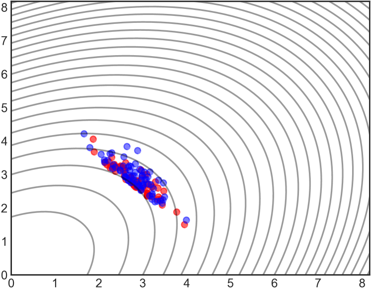
(a) Gaussian marginals, correlation$=0.5$

(b) Exponential marginals,
with $t-$copula

(c) Weibull marginals with $\boldsymbol{\alpha}=(0.5,0.5),$ uncorrelated

(d)

(e)

(f)

Figure 3. Figures (a) - (c) plot independent samples from the zero-variance distribution (in red) and that of the IS vector $\boldsymbol{Z}\,|\,L(\boldsymbol{Z})\geq u$ (in blue) to illustrate their identical concentration behaviour. Contours indicate the level sets of the respective joint distributions. Figures (d) - (f) show the respective histograms for $\boldsymbol{\kappa}^{(1)}(\boldsymbol{X})\ |\ L(\boldsymbol{Z})\geq u$ involved in the transformation $\boldsymbol{Z}=\boldsymbol{T}(\boldsymbol{X})$.

The zero variance and the IS samples tend to concentrate in the same neighbourhoods in all the three cases considered in Figures 3(a) - 3(c) as asserted by Proposition 5.1. Regardless of the distinctions in the regions where the zero variance distribution concentrates, the blue conditional IS samples replicate the concentration in the same neighbourhood.

To gain intuition behind this phenomenon, we first see that the multiplicative factor $(u/l)^{\boldsymbol{\kappa}^{(1)}(\boldsymbol{x})}\gg\boldsymbol{1}$ in the transformation $\boldsymbol{T}_{u}^{(1)}(\boldsymbol{x})=(u/l)^{\boldsymbol{\kappa}^{(1)}(\boldsymbol{x})}\boldsymbol{x}$ ensures that the IS vector $\boldsymbol{T}_{u}^{(1)}(\boldsymbol{X})$ is more likely to take more extreme values than $\boldsymbol{X}.$ Here the exponent $\boldsymbol{\kappa}^{(1)}(\boldsymbol{x})$ ensures that the components are relatively magnified only to the extent necessary. Indeed, a quick examination by applying the definition of $\boldsymbol{\kappa}^{(1)}(\boldsymbol{x})$ in (7) to the red points in the respective cases in Figure 3 reveals the following observation: The distribution of $\boldsymbol{\kappa}^{(1)}(\boldsymbol{X})\,|\,L(\boldsymbol{Z})\geq u$ concentrates in the neighbourhood of the points $\{(1,0),(0,1)\}$ in Figure 3(f), unlike those in Figures 3(d) - 3(e) where its concentration is in the vicinity of $(1,1).$ While a naive multiplication by the factor $(u/l)$ will result in both components $(X_{1},X_{2})$ being magnified, the introduction of $(u/l)^{\boldsymbol{\kappa}^{(1)}(\boldsymbol{X})}$ lets the conditional distribution of $\boldsymbol{Z}$ concentrate appropriately near the axes in the heavier-tailed case in Figure 3(c). Thus the transformation $\boldsymbol{T}_{u}^{(1)}(\cdot)$ is crucial here in adjusting the magnification of different components of $\boldsymbol{X}$ such that the transformed vector $\boldsymbol{Z}=\boldsymbol{T}_{u}^{(1)}(\boldsymbol{X})$ concentrates measure in the regions deemed suitable by the zero-variance IS distribution.

5.2. Logarithmic efficiency of Algorithm 1

Recall the IS estimator $\bar{\zeta}_{{}_{N}}(u)$ returned by Algorithm 1 is the sample mean computed from $N$ independent replications of the random variable,

$$\zeta(u):=\mathcal{L}(\boldsymbol{Z})\mathbb{I}\left(L(\boldsymbol{Z})\geq u\right),$$

where $\boldsymbol{Z}:=\boldsymbol{T}(\boldsymbol{X})$ and $\mathcal{L}(\boldsymbol{Z}):=J(\boldsymbol{X}){f_{\boldsymbol{X}}(\boldsymbol{Z})}/{f_{\boldsymbol{X}}(\boldsymbol{X})},$ with $J(\cdot)$ as the Jacobian of the map $\boldsymbol{T}(\cdot)$. Here the map $\boldsymbol{T}$ employed in Algorithm 1 can be seen to coincide with the rate-function preserving transformations (21) - (22) deduced in Section 5.1. Let $M_{2,u}:=E\big{[}\,\zeta(u)^{2}\,\big{]}$ denote the second moment of $\zeta(u).$ With $\bar{\zeta}_{{}_{N}}(u)$ being the average of $N$ independent samples of $\zeta(u),$ the variance of $\bar{\zeta}_{{}_{N}}(u)$ is given by $\left(M_{2,u}-p_{u}^{2}\right)N^{-1}.$ If one were to take the naive estimator $\mathbb{I}(L(\boldsymbol{X})>u),$ then as explained in Section 2.2, the resulting second moment is $p_{u}(1-p_{u})$ and the relative error scales as $p_{u}^{-1}.$ Theorem 5.1 below establishes that the second moment $M_{2,u}=o(p_{u}^{2-\varepsilon})$ for any $\varepsilon>0$, thereby offering nearly optimal variance reduction when considering the lower bound $M_{2,u}\geq p_{u}^{2}.$ In order to state Theorem 5.1, let us introduce a regularity condition on the marginal distributions of $\boldsymbol{X}.$

Assumption 5.1.

There exists $x_{0}>0$ such that for every $i=1,\ldots,d,$ the cumulative hazard function, $\Lambda_{i}(x)=-\log P(X_{i}>x),$ is either a convex or concave function over the interval $x\in[x_{0},\infty).$

The condition in Assumption 5.1 is readily satisfied for the examples in Tables 2 - 3 in Appendix B and for other commonly used probability distributions.

Theorem 5.1 (Logarithmic efficiency).

Suppose $\boldsymbol{X}$ satisfies Assumptions 3.1 - 5.1 and the limit $\boldsymbol{q}^{\ast}$ exists. For the loss $L(\cdot),$ suppose that $L(\cdot)$ satisfies Assumption 2.1 and the limiting function $L^{\ast}(\cdot)$ is such that $L^{\ast}(\boldsymbol{q}^{\ast}\boldsymbol{x})$ is not identically zero for $\boldsymbol{x}\in\mathbb{R}_{d}^{+}.$ Then for any choice of parameter $l$ in the IS transformation (4) which is taken to be slowly varying in $u,$ the family of estimators $\{\zeta(u):u>0\}$ is logarithmically efficient in estimating $p_{u}:=P(L(\boldsymbol{X})\geq u):$ that is,

$$\lim_{u\to\infty}\frac{\log M_{2,u}}{\log p_{u}^{2}}=1.$$ (23)

5.3. Log-efficiency in the presence of heavier-tailed distributions

Here we present the counterpart for Theorems 4.1 and 5.1 when one or more of the components of $X_{1},\ldots,X_{d}$ are heavier-tailed than considered in Assumption 3.1. Interestingly, the same Algorithm 1 is shown to offer asymptotically optimal variance reduction in the presence of heavier-tailed distributions. As in Section 3, we write $\Lambda_{i}(x)=-\log P(X_{i}>x),$ for $x\in\mathbb{R}.$ In addition, let

$$\bar{\Lambda}_{i}(x) :=-\log P(\log X_{i}>x)=\Lambda_{i}\circ\exp(x),\ x\in\mathbb{R}.$$

Assumption 5.2.

For any $i\in\{1,\ldots,d\}$ for which $\Lambda_{i}$ does not satisfy Assumption 3.1, $\bar{\Lambda}_{i}$ is continuous and strictly increasing in the interval $(x_{0},\infty)$, and $\bar{\Lambda}_{i}\in\mathscr{RV}(\alpha_{i}),$ for some $\alpha_{i}\in[1,\infty).$

Assumption 5.2 enriches Assumption 3.1 by including the possibility that, if the hazard function for $X_{i}$ is not regularly varying, then the hazard function for $\log X_{i}$ is instead regularly varying. This immediately brings commonly used heavier-tailed distributions such as log-normal, pareto and regularly varying distributions under the framework considered. Indeed, if $X_{i}$ is log-normally distributed, we have $\bar{\Lambda}_{i}(x)=x^{2}/2-\log x(1+o(1))$ satisfying $\bar{\Lambda}_{i}\in\mathscr{RV}(2).$ Instead, if $X_{i}$ is a pareto or regularly varying random variable, we have $\bar{\Lambda}_{i}(x)=\alpha x-\log L(e^{x}),$ for some $\alpha>0$ and a slowly varying function $L(\cdot);$ in this case, $\bar{\Lambda}_{i}\in\mathscr{RV}(1)$ (see Table 3). Since the case where all the components $X_{1},\ldots,X_{d}$ satisfy Assumption 3.1 is treated in the sections before, we proceed without any loss of generality by assuming here that there exists at least one component $X_{i}$ for which Assumption 3.1 is not satisfied. Let us assign

$$\hat{\boldsymbol{q}}(t):=\frac{\log\boldsymbol{q}(t\boldsymbol{1})}{\ \|\log\boldsymbol{q}(t\boldsymbol{1})\|_{\infty}},\quad\text{ and }\quad\boldsymbol{q}^{\ast}:=\lim_{t\rightarrow\infty}\hat{\boldsymbol{q}}(t),$$ (24)

if the limit exists. Here, $\boldsymbol{q}:\mathbb{R}_{+}^{d}\rightarrow\mathbb{R}^{d}$ denotes the component-wise inverse $\boldsymbol{q}(\boldsymbol{y})=(q_{1}(y_{1}),\ldots,q_{d}(y_{d})),$ with $q_{i}(y_{i})={\Lambda}_{i}^{\leftarrow}(y_{i})$ specifying the left-continuous inverse of the hazard function. We proceed assuming that the loss $L(\cdot)$ satisfies the following variation of Assumption 2.1.

Assumption 5.3.

Suppose that the function $L:\mathbb{R}^{d}\rightarrow\mathbb{R}_{+}$ satisfies Assumption 2.1 and the limiting function $L^{\ast}(\cdot)$ is such that $\lim_{n\rightarrow\infty}n^{-1}\log L^{\ast}\left(\exp(n\boldsymbol{x})\right)=\bar{L}^{\ast}(\boldsymbol{x}),$ for all $\boldsymbol{x}\in\mathbb{R}^{d}_{+}$ and some limiting function $\bar{L}^{\ast}:\mathbb{R}^{d}_{+}\rightarrow\mathbb{R}_{+}.$

For instance, in the examples considered earlier in Section 2, we have the resulting $\bar{L}^{\ast}(\boldsymbol{x})=\max\{x_{i}:i=1,\ldots,d\}$ and $\bar{L}^{\ast}(\boldsymbol{x})=2\max\{x_{i}:i=1,\ldots,d\}$ for the linear and quadratic losses in Examples 1-2.3 respectively. We have the following counterparts to Theorems 4.1 & 5.3 in the presence of heavier tailed distributions.

Theorem 5.2 (Tail asymptotic).

Suppose that the marginal distributions of the components $X_{1},\ldots,X_{d}$ of the random vector $\boldsymbol{X}=(X_{1},\ldots,X_{d})$ satisfy Assumption 5.2 and the standardized vector $\boldsymbol{Y}=\boldsymbol{\Lambda}(\boldsymbol{X})$ is such that the tail LDP in Theorem 3.1 holds. Further suppose that the limit $\boldsymbol{q}^{\ast}$ in (24) exists. Then for any $L(\cdot)$ satisfying Assumption 5.3,

$${\log P\left(L(\boldsymbol{X})\geq u\right)}=-{\Lambda_{\min}(u)}\big{(}I^{\ast}+o(1)\big{)},\quad u\rightarrow\infty$$ (25)

where the non-negative constant $I^{\ast}:=\inf\big{\{}I(\boldsymbol{y}):\bar{L}^{\ast}\big{(}{\boldsymbol{q}^{\ast}}\boldsymbol{y}^{\boldsymbol{1}/\boldsymbol{\alpha}}\big{)}\geq 1,\ \boldsymbol{y}\geq\boldsymbol{0}\big{\}}.$

Theorem 5.3 (Logarithmic efficiency of Algorithm 1 in the presence of heavier tails).

Suppose that the random vector $\boldsymbol{X}$ satisfies Assumptions 3.2 - 5.1, 5.2 and the limit $\boldsymbol{q}^{\ast}$ in (24) exists. For the loss $L(\cdot),$ suppose that $L(\cdot)$ satisfies Assumption 5.3 and the resulting limiting function $\bar{L}^{\ast}(\cdot)$ is such that $\bar{L}^{\ast}(\boldsymbol{q}^{\ast}\boldsymbol{x})$ is not identically zero for $\boldsymbol{x}\in\mathbb{R}_{d}^{+}.$ Taking $\rho=1$ and the choice $l$ in the IS transformation (4) to be slowly varying in $u,$ the second moment $M_{2,u}$ satisfies (23) and therefore the family of estimators $\{\zeta(u):u>0\}$ is logarithmically efficient.

While Theorems 5.1 & 5.3 prove asymptotically optimal variance reduction at the entire generality considered, we also point out that the proposed IS procedure is not suitable in its current form for example in certain tasks where Assumptions 1-4 are not satisfied: these include for example where $\boldsymbol{X}$ is a bounded random variable, or in tail estimation for steady-state simulation.

6. Application to Portfolio Credit Risk

Efficient IS schemes for estimating excess loss probabilities of a portfolio of loans have been considered in Glasserman & Li, (2005), Bassamboo et al., (2008), Glasserman et al., (2008). A salient feature of these approaches is the flexibility to have correlated loan defaults informed suitably via Gaussian or extremal copula models. The repertoire of loan default probability models considered in the literature since then have expanded to include machine learning based approaches aiming to capture more intricate interactions between the underlying covariates; see, for example, Sirignano & Giesecke, (2019), Sadhwani et al., (2020) and references therein. The treatment in this section capitalizes on the generic applicability of the proposed IS scheme to demonstrate how efficient samplers can be similarly devised in this setting.

To introduce the default model studied here, consider a portfolio of $m$ loans indexed by $\{1,\ldots,m\}$ belonging to $J\geq 1$ types. For any $i\in\{1,\ldots,m\}$, let $t(i)\in\{1,\ldots,J\}$ denote the type of loan $i$, $Y_{i}$ denote the indicator random variable that loan $i$ defaults over a fixed horizon of interest, $e_{i}$ denote the exposure upon its default, and $\boldsymbol{v}_{i}\in\mathbb{R}^{k}$ denote loan-specific factors (such as original interest rate, original loan-to-value, original debt-to-income ratios, FICO score, pre-payment penalty, etc.) which are fixed for a given loan. The average loss incurred by the portfolio is $L_{m}:=m^{-1}\sum_{i=1}^{m}e_{i}Y_{i}.$ If we let $\bar{e}_{m}:=m^{-1}\sum_{i=1}^{m}e_{i}$ denote the average of the exposures, then it is clear that $L_{m}\in(0,\bar{e}_{m}).$ For a given $q\in(0,1),$ our objective is to estimate the probability of the excess loss event,

$$\mathcal{E}_{m}:=\{L_{m}\geq q\bar{e}_{m}\},$$ (26)

which is the event that the incurred loss exceeds a given fraction of the maximum loss. To restrict the focus to main ideas, we take the exposure $e_{i}$ to be fixed for every $i\in\{1,\ldots,m\}$ and satisfy $e_{i}\in(0,e_{0}],$ where $e_{0}<\infty$ is the maximum exposure level.

The joint distribution of the default variables $Y_{1},\ldots,Y_{m}$ is taken to be determined by the loan-specific variables $\boldsymbol{v}_{1},\ldots,\boldsymbol{v}_{m}$ and some common stochastic factors $\boldsymbol{X}\in\mathbb{R}^{d}_{+}$ which affect all loans. The common factors $\boldsymbol{X}$ may capture region-level economic effects, such as those given by unemployment level, median income, etc., whose evolution is uncertain over the time horizon of interest. Conditioned on $\boldsymbol{X},$ the default indicators $Y_{1},\ldots,Y_{m}$ are taken to be independent and the respective conditional default probabilities are specified by the family of functions $\{W_{j}\}_{j=1,\ldots,J}$ as in,

$$P\left(Y_{i}=1\,|\,\boldsymbol{X}\right)=\frac{\exp\left(W_{t(i)}(\boldsymbol{X},\boldsymbol{v}_{i})-\gamma\right)}{1+\exp\left(W_{t(i)}(\boldsymbol{X},\boldsymbol{v}_{i})-\gamma\right)}\quad i=1,\ldots,m,$$ (27)

almost surely; in the above expression, $W_{j}:\mathbb{R}^{d}\times\mathbb{R}^{k}\rightarrow\mathbb{R}$ and $\gamma$ is a parameter modeling the rarity of loan defaults. While the functions $W_{j}(\cdot)$ are typically modeled as members of parametric families (see eg., Sirignano & Giesecke, 2019), we only require Assumption 6.1 below which is merely a restatement of Assumption 2.1b suitably adapted to this portfolio credit risk setting.

Assumption 6.1.

For $j\in\{1,\ldots,J\},$ the function $W_{j}:\mathbb{R}^{d}\times\mathbb{R}^{k}\rightarrow\mathbb{R}$ is such that for any sequence $\{\boldsymbol{x}_{n},\boldsymbol{v}_{n}\}_{n\geq 1}$ of $\mathbb{R}^{d}_{+}$ satisfying $(\boldsymbol{x}_{n},\boldsymbol{v}_{n})\rightarrow(\boldsymbol{x},\boldsymbol{v}),$ we have

$$\lim_{n\rightarrow\infty}\frac{W_{j}(n\boldsymbol{x}_{n},\boldsymbol{v}_{n})}{n^{\rho}}=W_{j}^{\ast}(\boldsymbol{x}),$$

where $\rho$ is a positive constant and $W_{j}^{\ast}:\mathbb{R}^{d}_{+}\rightarrow\mathbb{R}$ is the limiting function such that the cone $\{\boldsymbol{x}\in\mathbb{R}^{d}_{+}:W_{j}^{\ast}(\boldsymbol{x})>0\}$ is not empty.

The task of estimating $P(\mathcal{E}_{m})$ is particularly challenging in portfolios composed of high quality loans with small default probabilities. This rarity is specified, for example, in the default probabilities by letting the parameter $\gamma$ be large in (27). In order to study how an IS scheme fares when the target event becomes increasingly rare, we embed the given problem in the sequence of estimation problems indexed by $m,$ with $m\rightarrow\infty$ and the respective $\gamma$ in (27) and the exposures satisfying

$$\gamma m^{-\eta}\rightarrow c,\quad\bar{e}_{m}\rightarrow\bar{e},\quad\frac{1}{m}\sum_{i:t(i)=j}e_{i}\rightarrow\bar{c}_{j},$$ (28)

for some positive constants $c,\eta,\bar{e},\bar{c}_{j},$ $j=1,\ldots,J.$ Similar asymptotic frameworks form the basis of analysis in Glasserman & Li, (2005), Bassamboo et al., (2008), Glasserman et al., (2008); see Deo & Juneja, (2020) for a detailed exposition on the appropriateness of this regime in the context of logit default models. We impose a mild technical requirement that the parameter $q$ in (26) does not lie in the set $\{\bar{e}^{-1}\sum_{j\in I}\bar{c}_{j}:I\subseteq\{1,\ldots,J\}\}$. This unrestritive condition is common in the literature for ease of analysis; see Glasserman et al., (2007).

We first present a tail asymptotic for the excess loss probability $P(\mathcal{E}_{m})$ in Theorem 6.1 below as an application of Theorem 4.1. In order to state the result, let $\mathcal{J}_{m}$ denote the collection of subsets of the set $\{1,\ldots,J\}$ whose collective exposure exceeds the specified threshold; in other words, $\mathcal{J}_{m}:=\{I\subseteq\{1,\ldots,J\}:\sum_{i:\,t(i)\in I}e_{i}\geq mq\bar{e}_{m}\}.$ Let

$$L_{\textsc{cr}}(\boldsymbol{x}):=\max_{I\in\mathcal{J}_{m}}\min_{t(i)\in I}W_{t(i)}(\boldsymbol{x},\boldsymbol{v}_{i}),\quad\text{ and }\quad\mathcal{A}_{m}:=\left\{L_{\textsc{cr}}(\boldsymbol{X})>c(1-\varepsilon_{m})m^{\eta}\right\},$$ (29)

where $(\varepsilon_{m}:m\geq 1)$ is a sequence decreasing to zero as $m\rightarrow\infty.$ With the event $\mathcal{A}_{m}$ amenable to be treated via Theorem 4.1, Theorem 6.1 below establishes that the events $\mathcal{E}_{m}$ and $\mathcal{A}_{m}$ coincide as $m\rightarrow\infty$ and uses this observation to establish the asymptotic for $P(\mathcal{A}_{m})$ and $P(\mathcal{E}_{m}).$

Theorem 6.1 (Tail asymptotic for $P(\mathcal{E}_{m})$).

Suppose that the conditional default probabilities are specified as in (27), with the functions $W_{1}(\cdot),\ldots,W_{J}(\cdot)$ satisfying Assumption 6.1. In addition, suppose that the convergences in (28) hold and $\boldsymbol{X}$ satisfies the conditions in Theorem 4.1 with $\alpha_{\ast}:=\min_{i=1,\ldots,d}\alpha_{i}$ satisfying $\alpha_{\ast}<\rho(1+\eta^{-1}).$ Then as $m\rightarrow\infty,$

$$P\big{(}\mathcal{E}_{m}\setminus\mathcal{A}_{m}\big{)} =o\left(P(\mathcal{E}_{m})\right)\quad\text{ and }$$ (30)

$$\log P\left(\mathcal{E}_{m}\right)\sim\log P\left(\mathcal{A}_{m}\right) =-\Lambda_{\min}\big{(}m^{\eta/\rho}\big{)}\big{(}c^{\prime}I_{\textsc{cr}}+o(1)\big{)},$$

for any sequence $\varepsilon_{m}\rightarrow 0$ and $\varepsilon_{m}m^{\eta r/\rho}\rightarrow\infty,$ where $r<\rho(1+\eta^{-1})-\alpha_{\ast}.$ Here the constant $c^{\prime}:=c^{\alpha_{\ast}/\rho}$ and $I_{\textsc{cr}}$ are identified as,

$$I_{\textsc{cr}}:=\inf\big{\{}I(\boldsymbol{y}):\max_{I\in\mathcal{J}}\min_{k\in I}W_{k}^{\ast}(\boldsymbol{q}^{\ast}\boldsymbol{y}^{\boldsymbol{1}/\boldsymbol{\alpha}})\geq 1,\boldsymbol{y}\geq 0\big{\}},$$ (31)

in terms of $\mathcal{J}:=\{I\subseteq\{1,\ldots,J\}:\sum_{k\in I}\bar{c}_{k}\geq q\bar{e}\}$ and $\boldsymbol{q}^{\ast}$ specified as in Theorem 4.1.

Since the IS procedure introduced in Section 2.2 is readily applicable for estimating $P(\mathcal{A}_{m}),$ thanks to (30), one may suitably modify it to arrive at Algorithm 2 below which is efficient in estimating the desired excess loss probability $P(\mathcal{E}_{m}).$ The conditional sampling of default variables in Step 2a of Algorithm 2 involving exponential twisting is conventional (see, for eg., Glasserman, 2004, Chapter 9). The selection of a suitable IS distribution for the common factors $\boldsymbol{X},$ on the other hand, is often non-trivial (see eg., Glasserman et al., 2008) and is unknown if the functions $W_{j}(\cdot)$ modeling the default probabilities are specified generally, say, for example, in terms of a ReLU neural network as in Sirignano & Giesecke, (2019). This non-trivial task of arriving at a suitable IS distribution for $\boldsymbol{X}$ is however readily handled by the IS transformation $\boldsymbol{T}(\cdot)$ in Algorithm 2.

Input: Loss threshold $q\in(0,1),$ $N$ independent samples $\boldsymbol{X}_{1},\ldots,\boldsymbol{X}_{N}$ of $\boldsymbol{X}$, loan-specific values $\{\boldsymbol{v}_{1},\ldots,\boldsymbol{v}_{m}\},$ $u:=\gamma,$ hyper-parameter $l.$

Procedure:

1. Transform the samples and compute associated likelihood: Compute IS samples $\boldsymbol{Z}_{1},\ldots,\boldsymbol{Z}_{n}$ and their likelihoods $\mathcal{L}_{1},\ldots\mathcal{L}_{N}$ as described in Steps 1 - 2 of Algorithm 1.

2. Obtain samples of portfolio loss: For $k=1,\ldots,N,$ do the following steps:

• Generate the loan default variables $Y_{1,k},\ldots,Y_{m,k},$ where for $i=1,\ldots,m,$ $Y_{i,k}$ are independent Bernoulli random variable with success probability $\tilde{p}_{i}(\boldsymbol{Z}_{k}),$ where

  $$\tilde{p}_{i}(\boldsymbol{z}):=\frac{p_{i}(\boldsymbol{z})\exp(\lambda e_{i})}{1+p_{i}(\boldsymbol{z})(\exp(\lambda e_{i})-1)},$$ (32)

  $p_{i}(\boldsymbol{z}):=P(Y_{i}=1\ |\ \boldsymbol{X}=\boldsymbol{z})$ is as in (27), and $\lambda=\lambda_{m}(\boldsymbol{Z}_{k})$ in (32) is the unique solution of $\min_{\theta\geq 0}\{-\theta q\bar{e}_{m}+\psi_{m}(\theta,\boldsymbol{Z}_{k})\}$ with $\psi_{m}(\cdot,\boldsymbol{z})$ denoting the conditional cumulant

  $$\psi_{m}(\theta,\boldsymbol{z})={m}^{-1}\log\mathbb{E}\big{[}\exp(\theta mL_{m})|\ \boldsymbol{X}=\boldsymbol{z}\big{]}={m}^{-1}\sum_{i=1}^{m}\log\big{(}1+p_{i}(\boldsymbol{z})(\exp(\theta e_{i})-1)).$$

• Set $L_{m,k}:=m^{-1}\sum_{i=1}^{m}e_{i}Y_{i,k}$ to be the portfolio loss.

• Compute the conditional likelihood associated with the collection $\{Y_{1,k},\ldots,Y_{m,k}\}$ by letting $\mathcal{L}^{y}_{k}:=\exp\left(-m[\lambda_{m}(\boldsymbol{Z}_{k})L_{m,k}-\psi_{m}(\lambda_{m}(\boldsymbol{Z}_{k}),\boldsymbol{Z}_{k})]\right).$

3. Return the output estimator. Return the IS average computed as in,

$$\bar{\zeta}_{N}(m)=\frac{1}{N}\sum_{k=1}^{N}\mathcal{L}_{k}\mathcal{L}^{y}_{k}\ \mathbb{I}(L_{m,k}\geq q\bar{e}_{m}).$$

Algorithm 2 IS algorithm for estimating the excess loss probability $P(\mathcal{E}_{m})$

Proposition 6.1 (Log-efficiency of Algorithm 2).

Suppose that $\boldsymbol{X}$ satisfies the conditions in Theorem 5.1 and the density of $\boldsymbol{X}$ is bounded away from $0$ on compact subsets of $\mathbb{R}_{d}^{+}$. For the conditional default probabilities specified in (27), let the functions $W_{1}(\cdot),\ldots,W_{J}(\cdot)$ satisfy Assumption 6.1 and the resulting constant $I_{\textsc{cr}}$ in (31) is finite. Then under the asymptotic regime in (28) we have

$$\lim_{m\rightarrow\infty}\frac{\log E[\bar{\zeta}_{N}(m)^{2}]}{\log P(\mathcal{E}_{m})^{2}}=1,\qquad N\geq 1.$$

for any choice of the parameter $l$ which is slowly varying in $m.$ In other words, the family of unbiased estimators returned by Algorithm 2 is logarithmically efficient in estimating $P(\mathcal{E}_{m}).$

7. Numerical Experiments

We begin with a discussion on the selection of hyperparameter $l$ in Algorithm 1 before presenting the results of numerical experiments. Recall that the IS estimator returned by Algorithm 1 is unbiased for any choice of $l$ and the number of replications needed to attain a target relative precision is directly determined by the estimator variance. Therefore we seek to select $l$ which minimizes the sample average second moment estimate of the resulting IS estimator. Algorithm 3 below utilizes Retrospective Approximation (RA) for accomplishing this, as RA is effective in reducing the overall computational effort by balancing the errors due to sample based approximation of the objective and optimization (see Pasupathy, 2010). The RA procedure in Step 2 seeks to progressively increase the sample size $m_{k}$ employed, if required, while capitalizing on the current iterate $l_{k-1}$ to obtain an improved choice $l_{k}.$ An intermediate quantile of the distribution of $L(\boldsymbol{X})$ computed from a small pilot simulation run is used to obtain the initial choice $l_{0};$ as a rule of thumb, this may be chosen to be in the last two deciles of the distribution of $L(\boldsymbol{X})$. An advantage of our transformation based IS approach is that it requires obtaining samples only from the distribution of $\boldsymbol{X},$ and therefore the collection of samples in earlier steps get fully reused in successive steps of RA and in the computation of final IS estimate. In all the estimation tasks in Sections 7.1 - 7.2 below, we report results obtained for target relative precision requiring $\varepsilon=\alpha=0.05$ in Algorithm 3 and with the initialisation set to ${\tt tol}=q=0.1,m_{0}=500$, and $c=1.2$.

Step 0: Initialize sample size $m_{0}$ for pilot run, tolerance tol for terminating optimization, intermediate quantile level $q\in[0.1,30/m_{0}),$ $c>1,$ $\textsc{flag}_{i}=0,\ i=1,2.$

Step 1 (Pilot simulation run): Draw $m_{0}$ i.i.d. samples $\boldsymbol{X}_{1},\ldots\boldsymbol{X}_{m_{0}}$ of $\boldsymbol{X}.$ Assign $l_{0}=L_{(\lceil qm_{0}\rceil)},$ where $L_{(i)}$ is the $i$-th largest value in the collection $\{L(\boldsymbol{X}_{i}):i=1,\ldots,m_{0}\}.$

Step 2 (Retrospective Approximation): Set $k=1$. Do while $\textsc{flag}_{1}=0$,

• Set $m_{k}=\lceil cm_{k-1}\rceil$ and draw i.i.d. samples $\boldsymbol{X}_{m_{k-1}+1},\ldots,\boldsymbol{X}_{m_{k}}$ of $\boldsymbol{X}.$

Minimise second moment estimate $\textsc{sec-mom}(\boldsymbol{X}_{1},\ldots,\boldsymbol{X}_{m_{k}};l)$ numerically over $l$ with the initial iterate set to $l_{k-1}.$ Assign $M_{k}$ and $l_{k},$ respectively, to be the optimal value and the solution obtained by solving until the absolute error between successive iterates becomes smaller than $\varepsilon_{k}=m_{k}^{-1/2}$. The procedure $\textsc{sec-mom}(\boldsymbol{x}_{1},\ldots,\boldsymbol{x}_{k};l)$ for estimating second moment of the IS estimator given $l$ and a collection $\{\boldsymbol{x}_{1},\ldots,\boldsymbol{x}_{k}\},$ for any $k,$ is as follows:

procedure $\textsc{sec-mom}(\boldsymbol{x}_{1},\ldots,\boldsymbol{x}_{k};l)$

    For $i=1,\ldots,k,$ set $\boldsymbol{z}_{i}=(u/l)^{\boldsymbol{\kappa}(\boldsymbol{x}_{i})},\mathcal{L}_{i}=\frac{f_{\boldsymbol{X}}(\boldsymbol{z}_{i})}{f_{\boldsymbol{X}}(\boldsymbol{x}_{i})}J(\boldsymbol{x}_{i}),$ where $J(\boldsymbol{x})$ is as in Table 1.

    Return the second moment estimate $\hat{M}_{2}(l)=\frac{1}{k}\sum_{i=1}^{k}\mathcal{L}_{i}^{2}\mathbf{I}(L(\boldsymbol{z}_{i})\geq u).$

end procedure

If relative improvement $(M_{k}-M_{k-1})/M_{k-1}<{\tt tol},$ terminate while loop by setting $\textsc{flag}_{1}=1,$ choice of $l=l_{k},$ $\zeta_{i}=\mathcal{L}_{i}\mathbf{I}(L(\boldsymbol{Z}_{i})\geq u),$ with $\boldsymbol{Z}_{i}=(u/l)^{\boldsymbol{\kappa}(\boldsymbol{X}_{i})},$ $\mathcal{L}_{i}=\frac{f_{\boldsymbol{X}}(\boldsymbol{Z}_{i})}{f_{\boldsymbol{X}}(\boldsymbol{X}_{i})}J(\boldsymbol{X}_{i}),$ for $i\leq m_{k}$; else increment $k\leftarrow k+1.$

end while

Step 3 (Compute IS estimate with desired precision): Set $n=m_{k}+1$. Do while $\textsc{flag}_{2}=0$,

• Draw an independent sample $\boldsymbol{X}_{n}$ from the distribution of $\boldsymbol{X}.$ Set $\zeta_{n}=\mathcal{L}_{n}\mathbf{I}(L(\boldsymbol{Z}_{n})\geq u)$, where $\boldsymbol{Z}_{n}=\boldsymbol{X}_{n}(u/l)^{\boldsymbol{\kappa}(\boldsymbol{X}_{n})}$ and $\mathcal{L}_{n}=\frac{f_{\boldsymbol{X}}(\boldsymbol{Z}_{n})}{f_{\boldsymbol{X}}(\boldsymbol{X}_{n})}J(\boldsymbol{X}_{n})$. Evaluate $\bar{\zeta}_{n}(u)$ as the sample mean and $\hat{\sigma}$ as the sample standard deviation of the collection $\{\zeta_{i}:i\leq n\}$.

• If $\Phi^{-1}(1-\frac{\alpha}{2})\frac{\hat{\sigma}}{\sqrt{n}}<\bar{\zeta}_{n}(u)\varepsilon$, terminate loop by setting $\textsc{flag}_{2}=1$; else increment $n\leftarrow n+1$.

end while

Return $\bar{\zeta}_{n}(u)$ as the estimate for $P(L(\boldsymbol{X})\geq u).$

Algorithm 3 Combining IS with Retrospective Approximation based hyperparameter search for estimating $P(L(\boldsymbol{X})\geq u)$ within $\varepsilon$ relative error with $(1-\alpha)\times 100\%$-confidence

7.1. Illustration with the contextual shortest path problem

Here we employ the IS scheme for the contextual shortest path problem considered in Elmachtoub & Grigas, (2022). The goal is to travel from the north-west corner to the south-east corner of a $5\times 5$ grid. From any given vertex, only edges which travel south or east are available. Associated with each edge $j$ (enumerated as $\{1,\ldots 40\}$) is a traversing cost $C_{j}(\boldsymbol{S},\boldsymbol{\varepsilon})$ determined by contextual side information $\boldsymbol{S}$ and an additional random vector $\boldsymbol{\varepsilon}.$ The context $\boldsymbol{S}\in\mathbb{R}^{5}$ is taken to have independent Weibull marginals, with $F_{i}(x)=1-\exp(-x^{0.5}),$ for $1\leq i\leq 5$. The cost $C_{j}(\boldsymbol{S},\boldsymbol{\varepsilon})$ is given by,

$$\boldsymbol{C}(\boldsymbol{S},\boldsymbol{\varepsilon})=\big{[}5^{-1/2}(\boldsymbol{B}\boldsymbol{S}+\boldsymbol{3})^{\textrm{deg}}+\boldsymbol{1}\big{]}\boldsymbol{\varepsilon},$$ (33)

where $\boldsymbol{B}$ is a fixed $40\times 5$ matrix, $\text{deg}\in(0,\infty)$ allows nonlinear dependence on $\boldsymbol{S},$ and the independent noise $\boldsymbol{\varepsilon}$ has i.i.d. components uniformly distributed on $[1-a,1+a]$. The loss $L(\boldsymbol{C})=L(\boldsymbol{S},\boldsymbol{\varepsilon})$ is given as in (3), where $\boldsymbol{\Theta}$ is the shortest path polytope on the considered $5\times 5$ grid.

Experiment 1: We consider the estimation of $p_{u}:=P(L(\boldsymbol{C})\geq u),$ for values of $u$ resulting in $p_{u}\in[10^{-5.5},10^{-2.5}].$ The probability of large travel cost is estimated as in Algorithm 3 by averaging i.i.d. samples of $\mathcal{L}\boldsymbol{I}(L(\tilde{\boldsymbol{C}})\geq u),$ where $\tilde{\boldsymbol{C}}=\boldsymbol{C}(\boldsymbol{T}(\boldsymbol{S}),\boldsymbol{\varepsilon})$ is the IS cost vector and $\mathcal{L}$ is the respective likelihood ratio. Letting $V_{u}$ denote the sample variance of the collection $\{\mathcal{L}_{i}\boldsymbol{I}(L(\tilde{\boldsymbol{C}_{i}})\geq u):i\leq n\}$, we plot $\log V_{u}$ against $\log p_{u}$ in Figure 4(a) obtained for/ both the choices of $\boldsymbol{\kappa}$ in (7) and parameter choices $a=0.25,\text{ deg}=1.3.$ Note that the plot for IS variance is approximately a straight line with a slope of 2, supporting the conclusion $V_{u}=p_{u}^{2+o(1)}$ from Theorem 5.1. Naive sample averaging, on the other hand, can be seen to have orders of magnitude larger variance in Figure 4(a).

Experiment 2: Here we consider the predictive setting where a routing decision $\hat{\boldsymbol{\theta}}(\hat{\boldsymbol{C}})=\arg\min_{\boldsymbol{\theta}\in\boldsymbol{\Theta}}\boldsymbol{\theta}^{\intercal}\boldsymbol{\hat{C}}$ is obtained by plugging in the cost $\hat{\boldsymbol{C}}$ predicted from the realized contextual side information $\boldsymbol{S}.$ Note that while the realized cost $\boldsymbol{C}$ depends on both $\boldsymbol{S}$ and $\boldsymbol{\varepsilon},$ the realization of $\boldsymbol{\varepsilon}$ is not available at the time of decision-making. Suppose that similar to (Elmachtoub & Grigas, 2022, Section 6.1), the cost is predicted from a linear model $\hat{\boldsymbol{C}}={\boldsymbol{\hat{A}}}\boldsymbol{S};$ we take $\boldsymbol{\hat{A}}\in\arg\min\left\{10^{-3}\sum_{i=1}^{10^{3}}\left\|\boldsymbol{C}_{i}-\boldsymbol{A}\boldsymbol{S}_{i}\right\|_{2}^{2}\right\}$, estimated from historical data, $(\boldsymbol{S}_{1},\boldsymbol{C}_{1}),\ldots,(\boldsymbol{S}_{1000},\boldsymbol{C}_{1000}).$ The total cost realized by deploying the decision $\hat{\boldsymbol{\theta}}(\boldsymbol{C})$ is then given by $[\boldsymbol{\hat{\theta}}(\boldsymbol{\hat{C}})]^{\intercal}\boldsymbol{C},$ where the edge-traversal costs $\boldsymbol{C}$ satisfy (33). A risk manager is then naturally interested in evaluating tail risk probabilities such as in $p_{u}:=P([\boldsymbol{w}(\hat{\boldsymbol{C}})]^{\intercal}\boldsymbol{C}>u),$ that have to be borne from deploying the routing decision $\hat{\boldsymbol{\theta}}(\hat{\boldsymbol{C}}).$ Drawing samples for this purpose (drawn independently of those used to estimate ${\boldsymbol{\hat{A}}}$), we first generate the transformed tuple $(\boldsymbol{Z}_{i},\boldsymbol{\hat{D}}_{i},\boldsymbol{\tilde{C}}_{i})_{i\geq 1};$ here $\boldsymbol{Z}_{i}=\boldsymbol{T}(\boldsymbol{S}_{i})$ is the IS vector, $\boldsymbol{\tilde{\boldsymbol{C}}}_{i}=\boldsymbol{C}(\boldsymbol{Z}_{i},\boldsymbol{\varepsilon}_{i})$ and $\boldsymbol{\hat{D}}_{i}=\boldsymbol{\hat{A}}\boldsymbol{Z}_{i}$ serve as the realized and predicted costs, and $\hat{\boldsymbol{w}}(\hat{\boldsymbol{D}}_{i})$ denotes the respective shortest paths. Our IS estimator for the probability $p_{u}$ is then computed by averaging over $\{\mathcal{L}_{i}\boldsymbol{I}([\hat{\boldsymbol{w}}(\hat{\boldsymbol{D}}_{i})]^{\intercal}\boldsymbol{\tilde{C}}_{i})\geq u):i\leq n\}$ as in Step 3 of Algorithm 3. We plot $\log V_{u}$ (denoting the sample log variance) against $\log p_{u}$ in Figure 4(b) for the same parameter choices in Experiment 1. As before, we observe that the plot is approximately a straight line with a slope of $2$.

Figure 4(c) presents additional details on cross-validation by plotting the logarithm of estimator variance, $\log V_{u},$ observed (in red) for different choices of hyper-parameter $l$ considered. In Figure 4(c), the level $u=150$ is such that $p_{u}\approx 2\times 10^{-6}$. The high degree of variance reduction (exceeding 99.99%) in the interval $l\in(15,35)$ demonstrates that the estimator variance is not unduly sensitive to the choice of parameter $l.$ Further, we observe that Step 2 concludes after $m_{k}=2152$ samples and the estimated sample variance closely approximate the true variance. Thus $m_{k}$ can be seen to constitute only a fraction of the total sample requirement: for eg., a total of $n={16157}$ samples were required (on an average), in the estimation of $p_{u}\approx 10^{-4}$ with the stated precision.

(a) Estimation of $P(L(\boldsymbol{C})\geq u)$

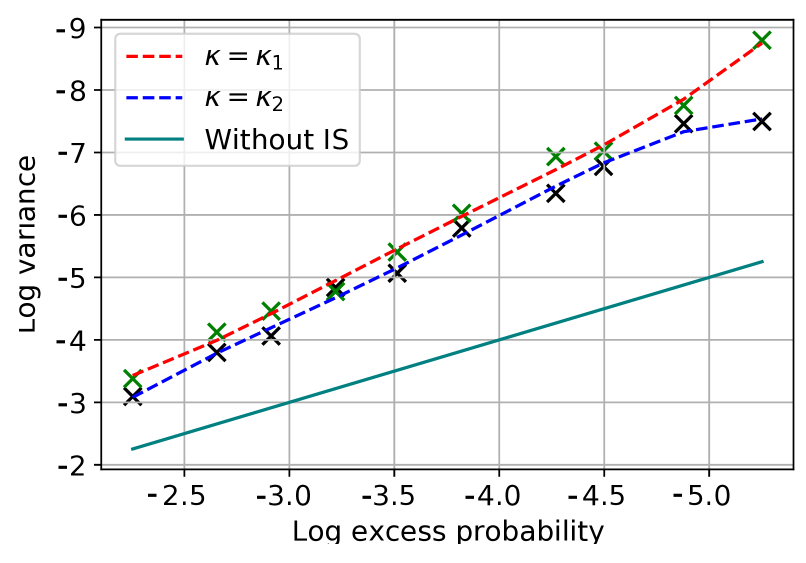
(b) Estimation of $P([\boldsymbol{w}(\hat{\boldsymbol{C}})]^{\intercal}\boldsymbol{C}\geq u)$

(c) $l$ vs second-moment $\hat{M}_{2}(l)$

Figure 4. Variance of the proposed IS estimator, illustrated via a log-log plot, for the contextual shortest path problem. Lines (solid and dashed) represent a polynomial fit to the variance values marked via crosses.

7.2. Illustration with the portfolio credit risk model

For the portfolio credit risk model considered in Section 6, we take a pool of $m=3000$ loans of a single type, each with an exposure $e_{i}=1.$ As in Section 7.1, the common factors $\boldsymbol{X}\in\mathbb{R}^{5}$ are taken to possess standard Weibull marginal distributions with shape parameter $0.8$. The dependence is informed by a Gaussian copula whose non-zero off-diagonal entries of the correlation matrix $R$ are taken to be $[R]_{i,j}=0.2,$ for $|j-i|=1.$ We consider cases where the conditional default probabilities are given by (a) the logit model in (27) and (b) the discrete default intensity of the form, $P(Y_{i}=1\,|\,\boldsymbol{X})=1-\exp(-\mathrm{e}^{W(\boldsymbol{X})-\gamma}).$ The function $W(\boldsymbol{x})=\boldsymbol{1}^{\intercal}(\boldsymbol{A}\boldsymbol{x}-\boldsymbol{b})^{+}$ is informed by a ReLU neural network with $1$ hidden layer with weights ${A}_{i,j}=1/5$ for all $(i,j)$ and $\boldsymbol{b}=\boldsymbol{0}.$

Taking the loss threshold $q=0.2$ in (26), we aim to estimate the probability of excess default loss $p_{\gamma}:=P(\mathcal{E}_{m});$ the parameter $\gamma$ in the conditional default probabilities dictate the rarity of loan defaults and is varied in the experiments so that the respective $p_{\gamma}$ varies from $10^{-2}$ to $10^{-5}.$ In Figure 5 below, we report $\log V_{\gamma}$ against $\log p_{\gamma},$ where $V_{\gamma}$ is the sample variance of the IS estimator. As in Section 7.1, the ratio between the logarithm of variance of IS estimator and that of the naive estimator (without IS) ranges over the interval $(1.6,1.9)$, which points to the IS estimator possessing negligible variance compared to that of sample averaging without IS.

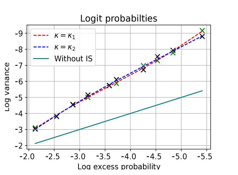
(a) Logit loan default probabilities

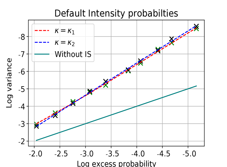
(b) Intensity based default probabilities

Figure 5. Plots displaying the logarithm of sample variance, $\log V_{\gamma},$ of the IS estimator versus $\log p_{\gamma},$ where $p_{\gamma}$ is excess default loss probability estimated.

7.3. Comparison with Cross-Entropy

In order to benchmark the number of samples and loss evaluations required by Algorithm 3 against a state-of-the-art adaptive IS algorithm, we compare its performance with that of cross-entropy. To this end, we consider evaluation of exceedence probabilities of (i) the PERT network loss from Rubinstein & Kroese, (2013) and (ii) neural network loss $W(\cdot)$ defined in Section 7.2. We assume that $\boldsymbol{X}$ has independent and exponential marginals. For cross-entropy, in line with the approach in Rubinstein & Kroese, (2013), we search for an IS distribution from among distributions with independent exponential marginals. For evaluation of probabilities using the proposed method, we use Algorithm 3. To facilitate a comparison of the two methods, we plot in Figure 6 the total number of samples required (across 30 independent experiments) to carry out the estimation to within a relative precision of $\varepsilon=0.05$ with confidence $\alpha=0.05$ using the respective method. Observe that in either setting, at a probability of $10^{-5}$, the sample requirement for the proposed IS is smaller by a factor exceeding $10^{3}.$ Further, cross-entropy method takes just under $10^{8}$ loss evaluations to cross-validate and compute the probabilities, while for the same task IS requires only about $10^{5}$.

(a) PERT Network

(b) Neural Network

Figure 6. Box-plots comparing sample requirements of cross-entropy method (in red) with those of the proposed sampler (in blue): Cross-entropy expends about $10^{3}$ times more effort than the proposed sampler.

Acknowledgements. Support from Singapore Ministry of Education’s AcRF Tier 2 grant MOE2019-T2-2-163 is gratefully acknowledged.We thank the anonymous reviewers and the Associate Editor for the insightful suggestions which have helped improve the paper in various respects.

The appendix is organized as follows: In Appendix A, we present the proofs of the main results Theorems 3.1 - 5.1. Appendix B serves to illustrate the wide applicability of the tail modeling framework with examples and sufficient conditions for Assumptions 3.1 - 3.2. Proofs of the results relating to portfolio credit risk applications, namely Proposition 6.1 and Theorem 6.1, are presented in Appendix C. Proofs of technical results (Lemma  3.1 - 3.2, Proposition 5.1 and Theorems 5.2 - 5.3) are given in Appendix D. Appendix E presents the proof of efficiency when $\boldsymbol{\kappa}=\boldsymbol{\kappa}_{2}$ is used in Algorithm 1. Appendix F outlines the verification of Assumption 2.1(b). Appendix G explores how the IS Algorithm 1 with the choice $\boldsymbol{\kappa}=\boldsymbol{\kappa}_{1}$ is well-suited for use in stochastic optimisation.

Appendix A Proofs of main results

The following definitions and notational convention are used in the proofs: For $r>0$ and $\boldsymbol{x}\in\mathbb{R}^{d},$ let $B_{r}(\boldsymbol{x})=\{\boldsymbol{y}\in\mathbb{R}^{d}:\|\boldsymbol{y}-\boldsymbol{x}\|\leq r\}$ denote the metric ball of radius $r$ around $\boldsymbol{x}.$ Unless specified explicitly, $\|\boldsymbol{x}\|=\max_{i=1,\ldots,d}|x_{i}|$ denotes the $\ell_{\infty}$-norm. Let $\mathcal{S}^{d-1}=\{\boldsymbol{x}\in\mathbb{R}^{d}:\|\boldsymbol{x}\|=1\}$ denote the unit sphere and $\mathbb{R}^{d}_{++}=\{\boldsymbol{x}\in\mathbb{R}^{d}:\boldsymbol{x}>0\}$ denote the interior of the positive orthant. For $M>0,$ let $B_{M}:=\{\boldsymbol{x}\in\mathbb{R}^{d}_{+}:\|\boldsymbol{x}\|\leq M\}.$ For $A\subseteq\mathbb{R}^{d}$, let $\mathrm{cl}(A)$ denote its closure, $\mathrm{int}(A)$ denote its interior,

$$\chi_{{}_{A}}(\boldsymbol{x}):=\begin{cases}0,\quad&\text{ if }\boldsymbol{x}\in A\\ +\infty,&\text{ otherwise},\end{cases}\qquad\text{ and }\qquad[A]^{1+r}:=\{\boldsymbol{x}+\boldsymbol{y}\in\mathbb{R}^{d}_{+}:\boldsymbol{x}\in A,\|\boldsymbol{y}\|\leq r\},$$

respectively denote the characteristic function and the set of points in $\mathbb{R}^{d}_{+}$ lying within a distance $r\in(0,\infty)$ from $A$. For $f:\mathbb{R}^{d}\rightarrow\mathbb{R},$ $\alpha\in\mathbb{R},$ $M>0,$ let

$$\textnormal{lev}_{\alpha}^{+}(f)=\{\boldsymbol{x}\in\mathbb{R}^{d}_{+}:f(\boldsymbol{x})\geq\alpha\}\quad\text{ and }\quad\Xi_{\alpha,M}(f)=\textnormal{lev}_{\alpha}^{+}(f)\cap B_{M}\cap\mathbb{R}^{d}_{++}$$

denote the super-level sets of $f$ restricted, respectively, to the positive orthant and to the bounded subset $B_{M}\cap\mathbb{R}^{d}_{++}.$ Recall that $\boldsymbol{Y}=\boldsymbol{\Lambda}(\boldsymbol{X}),$ the component-wise inverse $\boldsymbol{q}(t)=(\Lambda_{1}^{\leftarrow}(t),\ldots,\Lambda_{d}^{\leftarrow}(t)),$ and $\boldsymbol{q}^{\ast}=\lim_{t\rightarrow\infty}[\boldsymbol{q}(t)/q_{\infty}(t)],$ if the limit exists. Throughout the proofs, we suppose $u>x_{0}$ as specified in Assumption 2.1(a). Define $L_{u}:\mathbb{R}^{d}_{++}\rightarrow\mathbb{R}$ and $f_{\textnormal{LD}}:\mathbb{R}^{d}_{+}\rightarrow\mathbb{R}$ as,

$$L_{u}(\boldsymbol{x}):=u^{-1}{L(\boldsymbol{q}(t(u)\boldsymbol{x}))},\qquad f_{\textnormal{LD}}(\boldsymbol{y}):=L^{*}(\boldsymbol{q}^{*}\boldsymbol{y}^{\boldsymbol{1/\alpha}}),\text{ where }$$ (34a)

$$t(u):=\Lambda_{\min}\big{(}u^{1/\rho}\big{)}\quad\text{ and }\quad q_{\infty}(t):=\|\boldsymbol{q}(t)\|_{\infty},$$ (34b)

Write $\textrm{Diag}(\boldsymbol{a})$ for a diagonal matrix with diagonal entries $a_{1},\ldots,a_{d}$ and $\text{sgn}(\boldsymbol{x})$ for the vector of signs of $\boldsymbol{x}$. To avoid clutter in the expressions, define

$$\boldsymbol{Y}_{{u}}:={t(u)}^{-1}{\boldsymbol{Y}},\quad\boldsymbol{\psi}_{u}:=\boldsymbol{\Lambda}\circ\boldsymbol{T}^{-1}\circ\boldsymbol{q},\quad\text{ and }\quad c_{\rho}(u):=(l/u)^{1/\rho}.$$

where the parameter $u$ in the symbol $\boldsymbol{\psi}_{u}$ is explicitly indicated to remind the role of $u$ in $\boldsymbol{T}^{-1}.$

Proof of Theorem 3.1. A sufficient condition (see (Dembo & Zeitouni, 1998, Theorem 4.1.11)) to verify the existence of LDP is to show that for all $\boldsymbol{x}\in\mathbb{R}^{d}_{++},$

$$-I(\boldsymbol{x})=\inf_{\delta>0}\limsup_{t\to\infty}\frac{1}{t}\log P\left(\frac{\boldsymbol{Y}}{t}\in B_{\delta}(\boldsymbol{x})\right)=\inf_{\delta>0}\liminf_{t\to\infty}\frac{1}{t}\log P\left(\frac{\boldsymbol{Y}}{t}\in B_{\delta}(\boldsymbol{x})\right).$$ (35)

Fix any $\varepsilon,M\in(0,\infty)$ and $\boldsymbol{x}\in(0,M)^{d}.$ Since $f_{\boldsymbol{Y}}(\boldsymbol{y})=p(\boldsymbol{y})\exp(-\varphi(\boldsymbol{y})),$

$$P(\boldsymbol{Y}/t\in B_{\delta}(\boldsymbol{x}))=\int_{\boldsymbol{y}/t\in B_{\delta}(\boldsymbol{x})}p(\boldsymbol{y})\exp(-\varphi(\boldsymbol{y}))d\boldsymbol{y}=t^{d}\int_{\boldsymbol{z}\in B_{\delta}(\boldsymbol{x})}p(t\boldsymbol{z})\mathrm{e}^{-\varphi(t\boldsymbol{z})}d\boldsymbol{z}.$$

Recall that the continuous convergences in Assumption 3.2 imply the following uniform convergences over compact sets not containing the origin (see (Rockafellar & Wets, 1998, Theorem 7.14)):

$$n^{-1}\varphi(n\boldsymbol{x})\xrightarrow{n\to\infty}I(\boldsymbol{x})\text{ and }n^{-1}\log p(n\boldsymbol{x})\xrightarrow{n\to\infty}0.$$ (36)

Due to this local uniform convergence and the continuity of $I$, there exist $\delta_{0},t_{0}\in(0,\infty)$ such that,

$$\left|\frac{\varphi(t\boldsymbol{z})}{t}-I(\boldsymbol{x})\right|\leq\left|\frac{\varphi(t\boldsymbol{z})}{t}-I(\boldsymbol{z})\right|+\left|I(\boldsymbol{z})-I(\boldsymbol{x})\right|\leq\varepsilon/2,\textrm{ for all }\boldsymbol{z}\in B_{\delta}(\boldsymbol{x})$$

and $\exp(-\varepsilon t/2)\leq p(t\boldsymbol{z})\leq\exp(\varepsilon t/2),$ whenever $t>t_{0},$ $\delta<\delta_{0}$ and $B_{\delta_{0}}(\boldsymbol{x})$ does not contain the origin. Thus, given $\varepsilon,M$ and $\boldsymbol{x}\in(0,M)^{d},$ there exist $\delta_{0},t_{0}\in(0,\infty)$ such that for all $t>t_{0}$ and $\delta\in(0,\delta_{0}),$

$$\exp\left(-t(I(\boldsymbol{x})+\varepsilon)\right)\leq f_{\boldsymbol{Y}}(t\boldsymbol{z})\leq\exp\left({-t(I(\boldsymbol{x})-\varepsilon)}\right),\text{ uniformly over $\boldsymbol{z}\in B_{\delta}(\boldsymbol{x});$}$$ (37)

Then $t^{d}\mathrm{Vol}(B_{\delta}(\boldsymbol{x}))\exp({-t(I(\boldsymbol{x})+\epsilon)})\leq P(t^{-1}\boldsymbol{Y}\in B_{\delta}(\boldsymbol{x}))\leq t^{d}\mathrm{Vol}(B_{\delta}(\boldsymbol{x}))\exp({-t(I(\boldsymbol{x})-\epsilon)}).$ Since $P(\boldsymbol{Y}/t\in B_{\delta}(\boldsymbol{x}))$ is increasing in $\delta$ and these bounds hold for any $\delta<\delta_{0},$

$$-I(\boldsymbol{x})-\epsilon\leq\inf_{\delta>0}\liminf_{t\to\infty}\frac{1}{t}\log P(t^{-1}\boldsymbol{Y}\in B_{\delta}(\boldsymbol{x}))\leq\inf_{\delta>0}\limsup_{t\to\infty}\frac{1}{t}\log P(\boldsymbol{Y}/t\in B_{\delta}(\boldsymbol{x}))\leq-I(\boldsymbol{x})+\epsilon.$$

Since the choices $\varepsilon,M\in(0,\infty)$ are arbitrary, (35) holds. $\hfill\Box$

A.1. Proof of Theorem 4.1

For functions $f$ and $g$, let $f\land g$ (resp. $f\lor g$) denote their point-wise minimum (resp. maximum).

Lemma A.1.

Under Assumption 3.1, we have $q_{\infty}(t(u))=u^{1/\rho}.$ Therefore when Assumption 2.1 additionally holds, the events $\{L(\boldsymbol{X})\geq u\}$ and $\{\boldsymbol{Y}_{{u}}\in\textnormal{lev}^{+}_{1}(L_{u})\}$ coincide.

Proof. Consider increasing real valued functions $f_{1},f_{2}$. By the definition of left-continuous inverses, $(f_{1}\lor f_{2})^{\leftarrow}(y)=\inf\{u:f_{1}(u)\geq y\}\land\inf\{u:f_{2}(u)\geq y\}=f_{1}^{\leftarrow}(y)\land f_{2}^{\leftarrow}(y).$ From induction, $(\lor_{i=1}^{d}f_{i})^{\leftarrow}=\land_{i=1}^{d}f_{i}^{\leftarrow}$, given increasing functions $f_{1},\ldots,f_{d}$. Since $\{\Lambda_{i}:i=1,\ldots,d\}$ are continuous, $q_{i}^{\leftarrow}=\Lambda_{i}$ (see (de Haan & Ferreira, 2010, Excercise 1.1 (a))). Consequently,

$$q_{\infty}^{\leftarrow}(t)=\min_{i=1,…d}q_{i}^{\leftarrow}(t)=\Lambda_{\min}(t).$$ (38)

Then $q_{\infty}(\Lambda_{\min}(x))=x$ for all $x\in(x_{0},\infty)$ due to the strict monotonicity in Assumption 3.1. Since $\boldsymbol{q}=\boldsymbol{\Lambda}^{\leftarrow}$ is injective, $\{\boldsymbol{Y}_{{u}}\in A\}=\{\boldsymbol{X}\in\mathbf{q}(t(u)A)\},$ for any measurable $A$. With $L_{u}(\boldsymbol{x}):=u^{-1}L(\boldsymbol{q}(t(u)\boldsymbol{x})),$

$$\{\boldsymbol{q}(t(u)\boldsymbol{y}):\boldsymbol{y}\in\textnormal{lev}_{1}^{+}(L_{u})\}=\{\boldsymbol{q}(t(u)\boldsymbol{y}):L(\boldsymbol{q}(t(u)\boldsymbol{y}))\geq u\}=\{\boldsymbol{x}:L(\boldsymbol{x})>u\}\cap\textnormal{supp}(\boldsymbol{X}).\qquad\qquad{\Box}$$

Lemma A.2.

If Assumptions 2.1 and 3.1 hold and the limit $\boldsymbol{q}^{\ast}$ exists, the sequence of functions $\{L_{u}:u>0\}$ converge continuously to $f_{\textnormal{LD}}$ on $\mathbb{R}^{d}_{++}.$ Consequently, for any $\alpha,\varepsilon,M,K>0,$ there exists $u_{0}$ large enough such that for all $u>u_{0},$

$$\Xi_{\alpha,M}(L_{u})\subseteq\big{[}\Xi_{\alpha,M}(f_{\textnormal{LD}})\big{]}^{1+\varepsilon/2}\quad\text{ and }\quad\Xi_{\alpha+\varepsilon,M}(f_{\textnormal{LD}})\subseteq[\Xi_{\alpha+\varepsilon/2,M}(L_{u})]^{1+\varepsilon/K}$$

Proof. 1) Consider any sequences $\{u_{n}\}\subset\mathbb{R}_{+},\{\boldsymbol{x}_{n}\}\subset\mathbb{R}_{+}^{d}$ satisfying $u_{n}\uparrow\infty,\boldsymbol{x}_{n}\to\boldsymbol{x}>\boldsymbol{0}.$We rewrite,

$$L_{u_{n}}(\boldsymbol{x}_{n})=u_{n}^{-1}{L\left(\boldsymbol{q}(t(u_{n})\boldsymbol{x}_{n})/\boldsymbol{q}(t(u_{n})\boldsymbol{1})\cdot\hat{\boldsymbol{q}}(t(u_{n}))u_{n}^{1/\rho}\right)}.$$

Consider any $\delta>0$ such that $B_{\delta}(\boldsymbol{x})$ does not include $\boldsymbol{0}.$ As $\Lambda_{i}\in\mathscr{RV}(\alpha_{i}),$ we have $q_{i}\in\mathscr{RV}(1/\alpha_{i})$ (see Part 9 of (de Haan & Ferreira, 2010, Proposition B.1.9)). Due to the uniform convergence $\lim_{t\to\infty}\boldsymbol{q}(t\boldsymbol{y})/\boldsymbol{q}(t\boldsymbol{1})=\boldsymbol{y}^{\boldsymbol{1/\alpha}}$ over $\boldsymbol{y}\in B_{\delta}(\boldsymbol{x})$ (see (de Haan & Ferreira, 2010, Proposition B.1.4)),

$$\boldsymbol{q}(t(u_{n})\boldsymbol{x}_{n})/\boldsymbol{q}(t(u_{n})\boldsymbol{1})\to\boldsymbol{x}^{\boldsymbol{1/\alpha}},\text{ and }\hat{\boldsymbol{q}}(t(u_{n}))\to{\boldsymbol{q}^{*}},$$

Applying triangle inequality, $\boldsymbol{p}_{n}=\boldsymbol{q}(t(u)\boldsymbol{x}_{u})/\boldsymbol{q}(t(u)\boldsymbol{1})\hat{\boldsymbol{q}}(t(u))\to\boldsymbol{x}^{\boldsymbol{1/\alpha}}{\boldsymbol{q}}^{*}$. Continuous convergence

$$L_{u_{n}}(\boldsymbol{x}_{n}):=u_{n}^{-1}L(u_{n}^{1/\rho_{n}}\boldsymbol{p}_{n})\rightarrow L^{\ast}({\boldsymbol{q}}^{*}\boldsymbol{x}^{\boldsymbol{1/\alpha}})=:f_{\textnormal{LD}}(\boldsymbol{x})$$

follows from Assumption 2.1(b).

2) We next prove the claims on the set inclusions using the notions of $\limsup,\liminf$ of a sequence of sets defined in the Kuratowski sense (see (Rockafellar & Wets, 1998, Chapter 1)). Taking the ambient space $\mathcal{X}=\mathbb{R}^{d}_{++}$ in (Beer et al., 1992, Theorem 3.1), we obtain

$$\limsup_{u}\Xi_{\beta}(L_{u})\subseteq\Xi_{\beta}(f_{\textnormal{LD}}),\quad\liminf_{u}\Xi_{\beta_{u}}(L_{u})\supseteq\Xi_{\beta}(f_{\textnormal{LD}})\text{ for some $\beta_{u}\nearrow\beta$},$$ (39)

as a consequence of above verified $L_{u_{n}}(\boldsymbol{x}_{n})\rightarrow f_{\textnormal{LD}}(\boldsymbol{x}).$ Refer the construction in the proof of (Beer et al., 1992, Theorem 3.1) for using fixed level $\beta$ in the first set inclusion and considering increasing sequence $\beta_{u}$ in the second set inclusion in (39). Now, setting $\beta=\alpha$ in (39), using the equivalence between $(v)_{b}$ and $(vii)_{b}$ in (Salinetti & Wets, 1981, Theorem 2.2),

$$\Xi_{\alpha,M}(L_{u})\subseteq\big{[}\Xi_{\alpha,M}(f_{\textnormal{LD}})\big{]}^{1+\varepsilon/2}\cap\mathbb{R}^{d}_{++}\subseteq\big{[}\Xi_{\alpha,M}(f_{\textnormal{LD}})\big{]}^{1+\varepsilon/2}.$$

Set $\beta=\alpha+\varepsilon$, and let $\beta_{u}\nearrow\alpha+\varepsilon$ be selected as in (39). Therefore, for all large enough $u$, $\Xi_{\beta_{u},M}(L_{u})\subseteq\Xi_{\alpha+\varepsilon/2,M}(L_{u})$. From (39), $\Xi_{\alpha+\varepsilon,M}(f_{\textnormal{LD}})\subseteq\liminf_{u}\Xi_{\beta_{u}}(L_{u})\subseteq\liminf_{u}\Xi_{\alpha+\varepsilon/2,M}(L_{u}).$ Further, from the equivalence between $(vii)_{a}$ and $(v)_{a}$ in (Salinetti & Wets, 1981, Theorem 2.2),

$$\Xi_{\alpha+\varepsilon,M}(f_{\textnormal{LD}})\subseteq[\Xi_{\alpha+\varepsilon/2,M}(L_{u})]^{1+\varepsilon/K}\cap\mathbb{R}^{d}_{++}\subseteq[\Xi_{\alpha+\varepsilon/2,M}(L_{u})]^{1+\varepsilon/K}.\qquad\qquad{\Box}$$

Corollary A.1.

Suppose that Assumptions 2.1 and 3.1 hold and the limit $\boldsymbol{q}^{\ast}$ exists. Then for any $\alpha,\varepsilon,M>0,$ there exists $u_{0}$ large enough such that for all $u>u_{0},$

$$\textnormal{lev}_{\alpha}^{+}(L_{u})\cap B_{M}\subseteq\big{[}\Xi_{\alpha,M}(f_{\textnormal{LD}})\big{]}^{1+\varepsilon}\quad\text{ and }\quad\Xi_{\alpha+\varepsilon,M}(f_{\textnormal{LD}})\subseteq\Xi_{\alpha,M}(L_{u}).$$ (40)

Consequently, $\liminf_{n\rightarrow\infty}\chi_{\textnormal{lev}_{\alpha}^{+}(L_{u_{n}})}(\boldsymbol{x}_{n})\geq\chi_{\textnormal{lev}_{\alpha}^{+}(f_{\textnormal{LD}})}(\boldsymbol{x}),$ for any $\boldsymbol{x}_{n}\rightarrow\boldsymbol{x}$ and $u_{n}\rightarrow\infty.$

Proof. Notice that for $\varepsilon>0$, $\textnormal{lev}_{\alpha}^{+}(L_{u})\cap B_{M}\subseteq[\Xi_{\alpha,M}(L_{u})]^{1+\varepsilon/2}$, as a consequence of the definitions at the beginning of Section A. The first set inclusion now follows from the definition of the $[A]^{(1+r)}$ for a set $A\subset\mathbb{R}_{+}^{d}$. For the second set inclusion, observe that for $K>0$ (to be chosen imminently),

$$\Xi_{\alpha+\varepsilon,M}(f_{\textnormal{LD}})\subseteq[\Xi_{\alpha+\varepsilon/2,M}(L_{u})]^{1+\varepsilon/K}\cap\mathbb{R}^{d}_{++}$$

for all large enough $u$. Further, for any $\boldsymbol{x}$, $\boldsymbol{y}$,

$$|L_{u}(\boldsymbol{x})-L_{u}(\boldsymbol{y})|\leq|L_{u}(\boldsymbol{y})-f_{\textnormal{LD}}(\boldsymbol{y})|+|f_{\textnormal{LD}}(\boldsymbol{y})-f_{\textnormal{LD}}(\boldsymbol{x})|+|f_{\textnormal{LD}}(\boldsymbol{x})-L_{u}(\boldsymbol{x})|.$$

Recall that $L_{u}\to f_{\textnormal{LD}}$ uniformly on $\mathbb{R}_{++}^{d}\cap B_{2M}$ (see for example, (Rockafellar & Wets, 1998, Theorem 7.14)). Hence the first and third terms above may be made less than $\varepsilon/6$ for a large enough $u$ for any choices of $\boldsymbol{x},\boldsymbol{y}\in[\Xi_{\alpha+\varepsilon/2,M}(L_{u})]^{1+\varepsilon/K}\cap\mathbb{R}^{d}_{++}.$ Next, $f_{\textnormal{LD}}$ is uniformly continuous over $B_{2M}$. Therefore, there exists a $\kappa>0$, such that for $\boldsymbol{x},\boldsymbol{y}\in B_{2M}$, whenever $\|\boldsymbol{x}-\boldsymbol{y}\|\leq\kappa$, $|f_{\textnormal{LD}}(\boldsymbol{x})-f_{\textnormal{LD}}(\boldsymbol{y})|\leq\varepsilon/6$. Consider any $K\geq\varepsilon/\kappa.$ For any $\boldsymbol{y}\in[\Xi_{\alpha+\varepsilon/2,M}(L_{u})]^{1+\varepsilon/K}\cap\mathbb{R}_{++}^{d},$ there exists $\boldsymbol{x}\in\Xi_{\alpha+\varepsilon/2,M}(L_{u})$ such that $\|\boldsymbol{x}-\boldsymbol{y}\|\leq\kappa,$ and consequently,

$$|L_{u}(\boldsymbol{x})-L_{u}(\boldsymbol{y})|\leq\varepsilon/6+\varepsilon/6+\varepsilon/6\leq\varepsilon/2.$$

Therefore, whenever $\boldsymbol{y}\in[\Xi_{\alpha+\varepsilon/2,M}(L_{u})]^{1+\varepsilon/K}\cap\mathbb{R}_{++}^{d}$, $L_{u}(\boldsymbol{y})\geq\alpha$. Hence $\Xi_{\alpha+\varepsilon,M}(f_{\textnormal{LD}})\subseteq\Xi_{\alpha,M}(L_{u}).$
To verify the conclusion on characteristic functions, we proceed as follows: The bound in the statement is immediate if $\boldsymbol{x}\in\textnormal{lev}_{\alpha}^{+}(f_{\textnormal{LD}}),$ as $\chi_{\textnormal{lev}_{\alpha}^{+}(f_{\textnormal{LD}})}(\boldsymbol{x})=0$ in that case. Consider the case where $\boldsymbol{x}_{n}\rightarrow\boldsymbol{x}\notin\textnormal{lev}_{\alpha}^{+}(f_{\textnormal{LD}}).$ Then for a suitably small $\delta>0,$ $B_{\delta}(\boldsymbol{x})\cap[\textnormal{lev}_{\alpha}^{+}(f_{\textnormal{LD}})]^{1+\delta}=\varnothing,$ because of the continuity of $f_{\textnormal{LD}}$ and $\textnormal{lev}_{\alpha}^{+}(f_{\textnormal{LD}})$ being a closed set. Fix $M>\|\boldsymbol{x}\|+\delta.$ With $u_{n}\rightarrow\infty,$ we have

$$\textnormal{lev}_{\alpha}^{+}(L_{u_{n}})\cap B_{M}\subseteq\big{[}\Xi_{\alpha,M}(f_{\textnormal{LD}})\big{]}^{1+\delta}\subseteq\big{[}\textnormal{lev}_{\alpha}^{+}(f_{\textnormal{LD}})\cap B_{M}\big{]}^{1+\delta},\quad n>n_{0}$$

for sufficiently large $n_{0},$ due to the first inclusion in (40). For $n_{1}$ chosen large enough to ensure $\{\boldsymbol{x}_{n}\}_{n>n_{1}}\subseteq B_{\delta}(\boldsymbol{x}),$ we have $\{\boldsymbol{x}_{n}:n>n_{1}\}\cap[\textnormal{lev}_{\alpha}^{+}(f_{\textnormal{LD}})]^{1+\delta}=\varnothing.$ Consequently, $\boldsymbol{x}_{n}\notin\textnormal{lev}_{\alpha}^{+}(L_{u_{n}})\cap B_{M},$ for all $n>n_{2}:=\max\{n_{0},n_{1}\}.$ Since $M>\|\boldsymbol{x}\|+\delta$ and $\|\boldsymbol{x}_{n}\|\leq\|\boldsymbol{x}\|+\delta$ for $n>n_{2},$ $\boldsymbol{x}_{n}\notin\textnormal{lev}_{\alpha}^{+}(L_{u_{n}})\cap(\mathbb{R}^{d}\setminus B_{M})$ either. Therefore $\boldsymbol{x}_{n}\notin\textnormal{lev}_{\alpha}^{+}(L_{u_{n}})$ and $\chi_{\textnormal{lev}_{\alpha}^{+}(L_{u_{n}})}(\boldsymbol{x}_{n})=\infty$ for $n>n_{2}.$ $\Box$

Lemma A.3.

Suppose that $f,g:\mathbb{R}^{d}_{+}\rightarrow\mathbb{R}$ are continuous. For any $\alpha,\delta,M$ positive,

$$\inf_{\boldsymbol{x}\in[\Xi_{\alpha,M}(f)]^{1+\varepsilon}}g(\boldsymbol{x}) \geq\inf_{\boldsymbol{x}\in\textnormal{lev}^{+}_{\alpha}(f)\cap B_{M}}g(\boldsymbol{x})-\delta\quad\text{ and }$$

$$\inf_{\boldsymbol{x}\in\mathrm{int}(\Xi_{\alpha+\varepsilon,M}(f))}g(\boldsymbol{x}) \leq\inf_{\boldsymbol{x}\in\textnormal{lev}_{\alpha}^{+}(f)\cap B_{M}}g(\boldsymbol{x})+\delta,$$

for all $\varepsilon$ suitably small.

Proof. Observe that the sequence of sets $\mathcal{X}_{n}:=\{[\Xi_{\alpha,M}(f)]^{1+1/n}\}_{n\geq 1}$ are uniformly bounded in $n$ and $\cup_{i\geq 1}\mathcal{X}_{i}$ is relatively compact. Further, $\mathcal{X}_{n}\searrow\textnormal{lev}^{+}_{\alpha}(f)\cap B_{M}$ in the Kuratowski sense. Therefore, from (Langen, 1981, Theorem 2.2 (iii)), for all small enough $\epsilon$,

$$\inf_{\boldsymbol{x}\in[\Xi_{\alpha,M}(f)]^{1+\epsilon}}g(\boldsymbol{x})\geq\inf_{\boldsymbol{x}\in\textnormal{lev}_{\alpha}^{+}\cap B_{M}}g(\boldsymbol{x})-\delta.$$

In a similar spirit, due to the continuity of $f(\cdot)$, one has $\Xi_{\alpha+1/n,M}(f)\nearrow\Xi_{\alpha,M}(f).$ Then, upon an application of (Langen, 1981, Theorem 2.2 (iii)),

$$\inf_{\boldsymbol{x}\in\Xi_{\alpha+\varepsilon,M}(f)}g(\boldsymbol{x})\leq\inf_{\boldsymbol{x}\in\Xi_{\alpha,M}(f)}g(\boldsymbol{x})+\delta.$$

The statement then follows from the continuity of $g(\cdot).$ $\Box$

Proof of Theorem 4.1. Fix any $\delta,M>0.$ Observe that $I(\cdot)$ and $L^{\ast}(\cdot)$ are continuous. As a consequence of Lemma A.3, there exists $\varepsilon>0$ suitably small such that

$$\inf_{\boldsymbol{p}\in[\Xi_{1,M}(f_{\textnormal{LD}})]^{1+\epsilon}}I(\boldsymbol{p})\geq\inf_{\boldsymbol{p}\in\Xi_{1,M}(f_{\textnormal{LD}})}I(\boldsymbol{p})-\delta,\text{ and }$$ (41a)

$$\inf_{\boldsymbol{p}\in\mathrm{int}(\Xi_{1+\varepsilon,M}(f_{\textnormal{LD}}))}I(\boldsymbol{p})\leq\inf_{\boldsymbol{p}\in\textnormal{lev}_{1}^{+}(f_{\textnormal{LD}})\cap B_{M}}I(\boldsymbol{p})+\delta.$$ (41b)

Large deviations upper bound. Due to Lemma A.1,

$$P\big{(}L(\boldsymbol{X})\geq u\big{)} \leq P\big{(}\boldsymbol{Y}_{{u}}\in\textnormal{lev}^{+}_{1}(L_{u})\cap B_{M}\big{)}+P\big{(}\boldsymbol{Y}_{{u}}\in B_{M}^{c}\big{)}.$$ (42)

From Corollary A.1, $P\big{(}\boldsymbol{Y}_{{u}}\in\textnormal{lev}^{+}_{1}(L_{u})\cap B_{M}\big{)}\leq P\big{(}\boldsymbol{Y}_{{u}}\in\big{[}\Xi_{1,M}(f_{\textnormal{LD}})\big{]}^{1+\varepsilon}\big{)},$ for all $u$ sufficiently large. Since the expansion set $[A]^{1+r}$ is closed for any $A\subseteq\mathbb{R}^{d}_{+},$ the set $[\Xi_{\alpha,M}(f_{\textnormal{LD}})]^{1+\varepsilon}$ is closed. Therefore,

$$\limsup_{u\rightarrow\infty}\frac{1}{t(u)}\log P\big{(}\boldsymbol{Y}_{{u}}\in\textnormal{lev}^{+}_{1}(L_{u})\cap B_{M}\big{)} \leq\ \limsup_{u\rightarrow\infty}\frac{1}{t(u)}\log P\big{(}t(u)^{-1}\boldsymbol{Y}\in\big{[}\Xi_{1,M}(f_{\textnormal{LD}})\big{]}^{1+\varepsilon}\big{)}$$

$$\leq-\inf_{\boldsymbol{p}\in[\Xi_{1,M}(f_{\textnormal{LD}})]^{1+\varepsilon}}I(\boldsymbol{p})$$

$$\leq-\inf_{\boldsymbol{p}\in\textnormal{lev}^{+}_{1}(f_{\textnormal{LD}})\cap B_{M}}I(\boldsymbol{p})+\delta,$$

where the second inequality follows from the Tail LDP in Theorem 3.1 and the third inequality is a consequence of the choice of $\varepsilon$ satisfying (41a). Since $\delta>0$ is arbitrary,

$$\limsup_{u\rightarrow\infty}\frac{1}{t(u)}\log P\big{(}\boldsymbol{Y}_{{u}}\in\textnormal{lev}^{+}_{1}(L_{u})\cap B_{M}\big{)} \leq-\inf_{\boldsymbol{p}\in\textnormal{lev}^{+}_{1}(f_{\textnormal{LD}})\cap B_{M}}I(\boldsymbol{p})\leq-I^{\ast},$$

where $I^{\ast}:=\inf_{\boldsymbol{p}\in\textnormal{lev}^{+}_{1}(f_{\textnormal{LD}})}I(\boldsymbol{p}).$ A similar application of Theorem 3.1 results in

$$\limsup_{u\rightarrow\infty}\frac{1}{t(u)}\log P\left(\boldsymbol{Y}_{{u}}\in B_{M}^{c}\right)\leq-\inf_{\boldsymbol{p}\in\text{cl}(B_{M}^{c})}I(\boldsymbol{p})=-M,$$ (43)

where the latter inequality follows from Lemma 3.2d and the continuity of $I(\cdot).$ Combining these conclusions with that in (42) and (Dembo & Zeitouni, 1998, Lemma 1.2.15),

$$\limsup_{u\rightarrow\infty}\frac{1}{t(u)}\log P\left(L(\boldsymbol{X})\geq u\right)\leq-\min\left\{M,I^{\ast}\right\}.$$

Since $M$ can be made arbitrarily large, we have $\limsup_{u\rightarrow\infty}{t(u)}^{-1}\log P\left(L(\boldsymbol{X})\geq u\right)\leq-I^{\ast}.$
Large deviations lower bound. We have from Lemma A.1 and the definition of $\Xi_{\alpha,M}$ that $P(L(\boldsymbol{X})\geq u)\geq P(\boldsymbol{Y}_{{u}}\in\Xi_{1,M}(L_{u})).$ For $\varepsilon$ satisfying (41b), it follows from the second set inclusion in Corollary A.1 that $P(L(\boldsymbol{X})\geq u)\geq P(\boldsymbol{Y}_{{u}}\in\mathrm{int}\left(\Xi_{1+\varepsilon,M}(f_{\textnormal{LD}})\right)),$ for all sufficiently large enough $u.$ Then as an application of the tail LDP in Theorem 3.1,

$$\liminf_{u\to\infty}\frac{1}{t(u)}\log P(L(\boldsymbol{X})\geq u)\geq-\inf_{\boldsymbol{p}\in\mathrm{int}\left(\Xi_{1+\varepsilon,M}(f_{\textnormal{LD}})\right)}I(\boldsymbol{p})\geq-\inf_{\boldsymbol{p}\in\textnormal{lev}^{+}_{1}(f_{\textnormal{LD}})\cap B_{M}}I(\boldsymbol{p})-\delta,$$

where the latter inequality is a consequence of $\varepsilon$ satisfying (41b). Since $M,\delta$ are arbitrary,

$$\liminf_{u\rightarrow\infty}\frac{1}{t(u)}\log P\left(L(\boldsymbol{X})\geq u\right)\geq-\inf_{\boldsymbol{p}\in\textnormal{lev}^{+}_{1}(f_{\textnormal{LD}})}I(\boldsymbol{p})=-I^{\ast}.\qquad\qquad\Box$$

Remark A.1.

In the case where $L_{u}$ as defined in (34a) is independent of $u$, it can be seen that for a fixed map $\boldsymbol{Q}:\mathbb{R}^{d}_{+}\to\mathbb{R}_{d}^{+}$, $\boldsymbol{Q}(\textnormal{lev}_{1}^{+}(L_{u}))=\textnormal{lev}_{1}^{+}(f_{\textnormal{LD}})$. Thus, in such a case, Theorem 4.1 may be derived as a consequence of the contraction principle, rather than utilise the more elaborate machinery developed in Lemmas A.2-A.3. The former holds for example, if (i) $L(n\boldsymbol{x})=n^{\rho}L(\boldsymbol{x})$ for all $n,\boldsymbol{x}$ and (ii) $\boldsymbol{\Lambda}(\boldsymbol{x})=\boldsymbol{x}^{\boldsymbol{\alpha}}$ for some $\alpha>0$.

A.2. Proof of Proposition 2.1 and useful bounds on the inverse of $\boldsymbol{T}(\cdot).$

Proof of Proposition 2.1: First consider the case $\boldsymbol{\kappa}=\boldsymbol{\kappa}^{(1)}$. Let $k_{\rho}(u):=\log(u/l).$ It is sufficient to show that the determinant of the Jacobian of the map $\boldsymbol{x}\mapsto\boldsymbol{T}(\boldsymbol{x})$ equals $J(\boldsymbol{x})$. In that case, the density of $\boldsymbol{Z}$, denoted by $f_{\boldsymbol{Z}}(\cdot)$, is $f_{\boldsymbol{Z}}(\boldsymbol{T}(\boldsymbol{x}))=f_{\boldsymbol{X}}(\boldsymbol{x})/J(\boldsymbol{x})$; consequently, the likelihood ratio between the distributions of $\boldsymbol{Z}$ and that of $\boldsymbol{X}$ (or the Radon-Nikodym derivative evaluated at the samples $\boldsymbol{Z}_{1}\ldots\boldsymbol{Z}_{n}$) is given as in Algorithm 1. So the rest of the verification is devoted to checking that $J(\cdot)$ indeed equals the determinant of the Jacobian $\textrm{Jac}_{\boldsymbol{T}}(\cdot)=\partial\boldsymbol{T}/\partial\boldsymbol{x}.$ To this end, define $\boldsymbol{\psi}(\boldsymbol{x})=\log|\boldsymbol{x}|+k_{\rho}(u)\boldsymbol{\kappa}(\boldsymbol{\boldsymbol{x}})$ and observe that $\boldsymbol{T}(\boldsymbol{x})=\text{Diag}(\text{sgn}(\boldsymbol{x}))\mathrm{e}^{\boldsymbol{\psi}(\boldsymbol{x})}$. Now, following the chain rule for Jacobians,

$$\text{Jac}(\boldsymbol{x}) =\text{Diag}(\text{sgn}(\boldsymbol{x}))\mathrm{Diag}(\mathrm{e}^{\boldsymbol{\psi}(\boldsymbol{x})})\textrm{Jac}_{\psi}(\boldsymbol{x}),\textrm{ for almost every $\boldsymbol{x},$ and }$$

$$\textrm{Jac}_{\psi}(\boldsymbol{x}) =\mathrm{Diag}\left(\frac{\text{sgn}(\boldsymbol{x})}{|\boldsymbol{x}|}\right)+\rho^{-1}k_{\rho}(u)\left[\mathrm{Diag}\left(\frac{\text{sgn}(\boldsymbol{x})}{(1+|\boldsymbol{x}|)\|\log(1+|\boldsymbol{x}|)\|_{\infty}}\right)-\frac{\log(1+|\boldsymbol{x}|)}{\|\log(1+|\boldsymbol{x}|)\|_{\infty}^{2}}(\boldsymbol{e}^{*}/(1+|\boldsymbol{x}|))^{\intercal}\right]$$

$$=\mathrm{Diag}\left(\text{sgn}(\boldsymbol{x})\left[\frac{1}{|\boldsymbol{x}|}+\frac{\rho^{-1}k_{\rho}(u)}{(1+|\boldsymbol{x}|)\|\log(1+|\boldsymbol{x}|)\|_{\infty}}\right]\right)-\rho^{-1}k_{\rho}(u)\left[\frac{\log(1+|\boldsymbol{x}|)}{\|\log(1+|\boldsymbol{x}|)\|_{\infty}^{2}}(\boldsymbol{e}^{*}/(1+|\boldsymbol{x}|))^{\intercal}\right]$$

where $\boldsymbol{e}^{*}_{i}=\text{sgn}(x_{i})$ if $|x_{i}|=\|\boldsymbol{x}\|_{\infty}$, and $\boldsymbol{e}^{*}_{i}=0$ otherwise. Notice that for this component, $\|\boldsymbol{x}\|_{\infty}=|x_{i}|$. Now, recall that if $M=A+\mathbf{u}\mathbf{v}^{\intercal}$, then $|M|=(1+\mathbf{u}^{\intercal}A^{-1}\mathbf{v})|A|$. Set

$$\boldsymbol{u} =\log(1+|\boldsymbol{x}|)/\|\log(1+|\boldsymbol{x}|)\|_{\infty}^{2},\quad\boldsymbol{v}=-(k_{\rho}(u)\boldsymbol{e}^{*}/(1+|\boldsymbol{x}|))^{\intercal},\text{ and}$$

$$A =\mathrm{Diag}\left(\text{sgn}(\boldsymbol{x})\left[\frac{1}{|\boldsymbol{x}|}+\frac{k_{\rho}(u)}{(1+|\boldsymbol{x}|)\|\log(1+|\boldsymbol{x}|)\|_{\infty}}\right]\right).$$

Then, almost everywhere,

$$1+\boldsymbol{u}^{\intercal}A^{-1}\boldsymbol{v} =1-\frac{\rho^{-1}k_{\rho}(u)\|\boldsymbol{x}\|_{\infty}}{\|1+|\boldsymbol{x}|\|_{\infty}\|\log(1+|\boldsymbol{x}|)\|_{\infty}+k_{\rho}(u)\|\boldsymbol{x}\|_{\infty}},\text{ and }$$

$$|A| =\prod_{i=1}^{d}\frac{1}{|x_{i}|}\times\prod_{i=1}^{d}\left(1+\frac{\rho^{-1}k_{\rho}(u)|x_{i}|}{(1+|x_{i}|)\|\log(1+|\boldsymbol{x}|)\|_{\infty}}\right).$$

To complete the verification, observe $|\mathrm{Diag}(\mathrm{e}^{\boldsymbol{\psi}(\boldsymbol{x})})|=\prod_{i=1}^{d}|x_{i}|\cdot(u/l)^{\boldsymbol{1}^{\intercal}\boldsymbol{\kappa}(\boldsymbol{x})}$.
We next show that $\boldsymbol{T}(\cdot)$ is onto. Fix a $\boldsymbol{y}\in\mathbb{R}^{d}_{+}$. Let $I=\{i:y_{i}=\|\boldsymbol{y}\|_{\infty}\}$. Define the set,

$$S=\{\boldsymbol{x}:x_{i}=\|\boldsymbol{y}\|_{\infty}c_{\rho}(u)\textrm{ for all }i\in I,\,x_{i}\in[0,\|\boldsymbol{y}\|_{\infty}c_{\rho}(u)],\,i\not\in I\},$$ (44)

where recall $c_{\rho}(u):=(l/u)^{1/\rho}.$ Notice that for all $\boldsymbol{x}\in S,$

$$\boldsymbol{T}_{i}(\boldsymbol{x})=\begin{cases}x_{i}[c_{\rho}(u)]^{\frac{-\log(1+x_{i})}{\log(1+c_{\rho}(u)\|\boldsymbol{y}\|_{\infty})}}&\textrm{ for }i\not\in I,\\ \|\boldsymbol{y}\|_{\infty}&\textrm{ for }i\in I.\end{cases}$$

Restricted to $\boldsymbol{x}\in S$, $\boldsymbol{T}_{i}(\boldsymbol{x})$ is only a function of $x_{i}$ for $i\not\in I$. Fixing $i\notin I,$ see that $\boldsymbol{T}_{i}(\boldsymbol{x})<y_{i}$, if $x_{i}<y_{i}c_{\rho}(u);$ and $\boldsymbol{T}_{i}(\boldsymbol{x})=\|\boldsymbol{y}\|_{\infty}>y_{i}$ if $x_{i}=\|\boldsymbol{y}\|_{\infty}c_{\rho}(u).$ Since $\boldsymbol{T}_{i}$ are all continuous maps, by the intermediate value theorem, there exists some $\boldsymbol{x}^{\prime}\in[\boldsymbol{y}c_{\rho}(u),\|\boldsymbol{y}\|_{\infty}c_{\rho}(u)]^{d}$ such that $\boldsymbol{T}(\boldsymbol{x}^{\prime})=\boldsymbol{y}.$ The above argument also shows that if $\boldsymbol{x}_{1}\neq\boldsymbol{x}^{\prime}$, $\boldsymbol{T}(\boldsymbol{x}_{1})\neq\boldsymbol{T}(\boldsymbol{x}^{\prime})=\boldsymbol{y}$, that is, $\boldsymbol{T}(\cdot)$ is $1\leftrightarrow 1$. Since $\boldsymbol{T}(\cdot)$ is symmetric about the origin, one can similarly extend the proof to the case where $\boldsymbol{y}\in\mathbb{R}^{d}$.

Now suppose that $\boldsymbol{\kappa}=\boldsymbol{\kappa}^{(2)}$. Here, observe that by a direct application of the chain rule,

$$\left[\frac{\partial\boldsymbol{\kappa}(\boldsymbol{x})}{\partial\boldsymbol{x}}\right]=\text{Diag}\left(\frac{\log(u/l)}{\log l}\frac{\text{sgn}(\boldsymbol{x})}{1+|\boldsymbol{x}|}\right).$$

Substituting in the expression for the Jacobian in (9) completes the proof. $\Box$

In Lemmas A.4 and A.5 below, assume that $\boldsymbol{\kappa}=\boldsymbol{\kappa}^{(1)}$:

Lemma A.4.

For any $\boldsymbol{y}\in\mathbb{R}^{d}_{+}$ satisfying $\|\boldsymbol{y}\|_{\infty}\geq 1/c_{\rho}(u),$

$$\boldsymbol{y}c_{\rho}(u)\leq\boldsymbol{T}^{-1}(\boldsymbol{y})\leq\min\left\{\boldsymbol{y}[c_{\rho}(u)]^{\frac{\log\boldsymbol{y}}{\log\|\boldsymbol{y}\|_{\infty}}}\boldsymbol{\lor 1},\|\boldsymbol{y}\|_{\infty}c_{\rho}(u)\right\}.$$ (45)

Proof. We verify the bounds by exhibiting $\boldsymbol{x}^{\prime}$ sandwiched component-wise between the left and right hand sides of (45) and satisfying $\boldsymbol{T}(\boldsymbol{x}^{\prime})=\boldsymbol{y}.$ For any $\boldsymbol{y}$ as in the statement, we first set

$$\tilde{x}_{i}=\begin{cases}y_{i}\left[c_{\rho}(u)\right]^{\frac{\log y_{i}}{\log\|\boldsymbol{y}\|_{\infty}}}&\text{ if }y_{i}\geq 1,\\ 1&\text{ otherwise,}\end{cases}$$ (46)

for $i=1,\ldots,d.$ See that $\tilde{x}_{i}\in[1,\|\boldsymbol{y}\|_{\infty}c_{\rho}(u)].$ This is because of the following two observations: 1) $\log\tilde{x}_{i}=\left(1+\log c_{\rho}(u)/\log\|\boldsymbol{y}\|_{\infty}\right)\log y_{i}\geq 0,$ when $\|\boldsymbol{y}\|_{\infty}\geq 1/c_{\rho}(u)>1;$ and 2) likewise,

$$\log\tilde{x}_{i}-\log(\|\boldsymbol{y}\|_{\infty}c_{\rho}(u)) =\left(1+\frac{\log c_{\rho}(u)}{\log\|\boldsymbol{y}\|_{\infty}}\right)\left(\log y_{i}-\log\|\boldsymbol{y}\|_{\infty}\right)\leq 0.$$

Set $I=\{i:y_{i}=\|\boldsymbol{y}\|_{\infty}\}.$ With the set $S$ defined as in (44), we thus have $\tilde{\boldsymbol{x}}=(\tilde{x}_{1},\ldots,\tilde{x}_{d})\in S$ and $\tilde{x}_{i}\geq 1$ for all $i.$ Since $\log(1+t)/\log(t)$ is decreasing over $t\geq 1,$ we have

$$\boldsymbol{T}_{i}(\boldsymbol{x})=x_{i}[c_{\rho}(u)]^{-\frac{\log(1+x_{i})}{\|\log(1+\boldsymbol{x})\|_{\infty}}}\geq x_{i}[c_{\rho}(u)]^{{}^{\frac{-\log x_{i}}{\ \log\|\boldsymbol{x}\|_{\infty}}}},$$ (47)

for any $\boldsymbol{x}$ such that $x_{i}\geq 1,i=1,\ldots,d.$ With $\tilde{\boldsymbol{x}}$ defined via (46), we obtain the following from the bound in (47) and the observation $(\log\tilde{x}_{i})/(\log\|\tilde{\boldsymbol{x}}\|_{\infty})=(\log y_{i})/(\log\|\boldsymbol{y}\|_{\infty}):$

$$\boldsymbol{T}_{i}(\tilde{\boldsymbol{x}})=\begin{cases}\boldsymbol{T}_{i}(y_{i}[c_{\rho}(u)]^{\frac{\log y_{i}}{\log\|\boldsymbol{y}\|_{\infty}}})&\textrm{ if }y_{i}\geq 1,\\ \boldsymbol{T}_{i}(1)&\text{ otherwise},\end{cases}\quad\geq\ \begin{cases}y_{i}&\textrm{ if }y_{i}\geq 1,\\ 1&\text{ otherwise}.\end{cases}$$

For $i\notin I,$ the map $\boldsymbol{T}_{i}(\boldsymbol{x}),$ when restricted to $\boldsymbol{x}\in S,$ is a function only of $x_{i}$ and satisfies $\boldsymbol{T}_{i}(\tilde{\boldsymbol{x}})\geq y_{i}$ (regardless of whether $y_{i}>1$ or $y_{i}<1$). Applying the intermediate value theorem component-wise, we see that there exists some $x_{i}^{\prime}$ in the interval $[y_{i}c_{\rho}(u),\tilde{x}_{i}]$ containing $y_{i}$ such that $T_{i}(x_{i}^{\prime})=y_{i}$ for all $i\not\in I$. Setting $x_{i}^{\prime}=\|\boldsymbol{y}\|_{\infty}c_{\rho}(u)$ for $i\in I,$ we obtain $\boldsymbol{T}(\boldsymbol{x}^{\prime})=\boldsymbol{y}.$ Hence the bounds (45) hold. $\Box$

Lemma A.5.

Suppose that Assumptions 3.1 - 3.2 hold, $l(u)$ is slowly varying in $u$, and $\lim_{u\rightarrow\infty}l(u)=\infty.$ Then for any $\gamma>0$, the below convergence holds uniformly over $\boldsymbol{p}$ in compact subsets of $\mathbb{R}^{d}_{++}:$

$$\|\psi_{u}(t(u)\boldsymbol{p})\|_{\infty}=o(t(u)),\text{ as }u\rightarrow\infty.$$

Proof. Recall $\psi_{u}:=\boldsymbol{\Lambda}\circ\boldsymbol{T}^{-1}\circ\boldsymbol{q},$ $c_{\rho}(u):=(l(u)/u)^{1/\rho}$ and $q_{\infty}(t(u)):=\|\boldsymbol{q}(t(u))\|_{\infty}.$ Fix any $M>0,\gamma\in(0,M)$ and $\boldsymbol{p}\in B_{M}\setminus B_{\gamma}.$ As $\lim_{u\rightarrow\infty}l(u)=+\infty,$ $\boldsymbol{q}\in\mathscr{RV},$ and $q_{\infty}(t(u))=u^{1/\rho}$ (see Lemma A.1),

$$\|\boldsymbol{q}(t(u)\boldsymbol{p})\|_{\infty}c_{\rho}(u)=l(u)^{1/\rho}\frac{\|\boldsymbol{q}(t(u)\boldsymbol{p})\|_{\infty}}{\|\boldsymbol{q}(t(u))\|_{\infty}}\rightarrow\infty.$$ (48)

Then from (45), $\boldsymbol{T}^{-1}_{i}(\boldsymbol{q}(t(u)\boldsymbol{p}))\leq\|\boldsymbol{q}(t(u)\boldsymbol{p})\|_{\infty}c_{\rho}(u)\leq\|\boldsymbol{q}(t(u)M\boldsymbol{1})\|_{\infty}c_{\rho}(u),$ for $i=1,\ldots,d,$ as $\boldsymbol{q}$ is monotone and $\|\boldsymbol{p}\|_{\infty}\leq M$. With $q_{\infty}(t(u))=u^{1/\rho},$

$$\boldsymbol{q}(t(u)M\boldsymbol{1})c_{\rho}(u)=\frac{\boldsymbol{q}(t(u)M\boldsymbol{1})}{\boldsymbol{q}(t(u))}\frac{\boldsymbol{q}(t(u))}{q_{\infty}(t(u))}l(u)^{1/\rho}\leq\frac{\boldsymbol{q}(t(u)M\boldsymbol{1})}{\boldsymbol{q}(t(u))}l(u)^{1/\rho}.$$

Since $\boldsymbol{q}\in\mathscr{RV}(\boldsymbol{1/\alpha}),$ we have $\boldsymbol{q}(t(u)M\boldsymbol{1})c_{\rho}(u)\leq M^{\boldsymbol{1/\alpha}}l(u)^{1/\rho}(\boldsymbol{1}+o(\boldsymbol{1})).$ Therefore,

$$\boldsymbol{T}^{-1}_{i}(\boldsymbol{q}(t(u)\boldsymbol{p}))\leq\|\boldsymbol{q}(t(u)M\boldsymbol{1})\|_{\infty}c_{\rho}(u)\leq\max_{i=1,\ldots,d}M^{1/\alpha_{i}}l(u)^{1/\rho}({1}+o({1})),$$

uniformly over $\boldsymbol{p}\in B_{M}\setminus B_{\gamma}(\boldsymbol{0}).$ Recall $\boldsymbol{\Lambda}\in\mathscr{RV}(\boldsymbol{\alpha})$ is monotone. Write $\bar{\alpha}=\max_{i}\alpha_{i}.$ Then for $\delta>0,$

$$\|\boldsymbol{\psi}_{u}(t(u)\boldsymbol{p}))\|_{\infty}=\max_{i=1,\ldots,d}{\Lambda}_{i}\left(\boldsymbol{T}^{-1}_{i}(\boldsymbol{q}(t(u)\boldsymbol{p}))\right)\leq(1+\delta)M_{0}l(u)^{\bar{\alpha}/\rho+\delta},$$

for all $u$ sufficiently large (see (de Haan & Ferreira, 2010, Proposition B.1.9 (7))). Here $M_{0}>0$ is a suitably large constant. Since $t(u)=\Lambda_{\min}(u^{1/\rho}),$ noting $l(u)^{\bar{\alpha}/\rho+\delta}=o(t(u))$ completes the proof. $\Box$

A.3. Proof of Theorem 5.1 with $\boldsymbol{\kappa}=\boldsymbol{\kappa_{1}}$

Here, we demonstrate the proof of Theorem 5.1 in the case where $\boldsymbol{\kappa}=\boldsymbol{\kappa}_{1}$. The proof for $\boldsymbol{\kappa}=\boldsymbol{\kappa}_{2}$ is outlined in E. Unless explicitly specified, the only assumption made in the proofs below is that $\boldsymbol{X}$ has a probability density $f_{\boldsymbol{X}}(\cdot).$ As a consequence, the hazard rates

$$\lambda_{i}(x)=f_{X_{i}}(x)/\Lambda_{i}(x),\quad i=1,\ldots,d$$

are well-defined. In the above, $f_{X_{i}}(\cdot)$ denotes the probability density of the component $X_{i}.$

Lemma A.6.

The second moment $M_{2,u}=\mathbb{E}[\exp(-t(u)F_{u}(\boldsymbol{Y}_{{u}}))],$ where $F_{u}:\mathbb{R}^{d}_{+}\rightarrow\mathbb{R}\cup\{+\infty\}$ is,

$$F_{u}(\boldsymbol{p}):=a_{u}(\boldsymbol{p})+b_{u}(\boldsymbol{p})-2d\frac{\log t(u)}{t(u)}+\chi_{\textnormal{lev}^{+}_{1}(L_{u})}(\boldsymbol{p}),$$

for $u>0,$ and $a_{u}:\mathbb{R}^{d}_{+}\rightarrow\mathbb{R},$ $b_{u}:\mathbb{R}^{d}_{+}\rightarrow\mathbb{R}$ are defined as follows:

$$a_{u}(\boldsymbol{p}) =\frac{1}{t(u)}\left[\log f_{\boldsymbol{Y}}(\boldsymbol{\psi}_{u}(t(u)\boldsymbol{p})-\log f_{\boldsymbol{Y}}(t(u)\boldsymbol{p})\right],$$

$$b_{u}(\boldsymbol{p}) =\frac{1}{t(u)}\left[\sum_{i=1}^{d}\left[\log\lambda_{i}(\boldsymbol{T}^{-1}_{i}(\boldsymbol{q}(t(u)\boldsymbol{p})))-\log\lambda_{i}(q_{i}(t(u)p_{i}))\right]-\log J(\boldsymbol{T}^{-1}(\boldsymbol{q}(t(u)\boldsymbol{p})))\right].$$

Proof. Since the change of measure is effected by the map $\boldsymbol{Z}=\boldsymbol{T}(\boldsymbol{X}),$

$$M_{2,u} ={\mathbb{E}}\left[\left(\frac{f_{\boldsymbol{X}}(\boldsymbol{Z})}{{f}_{\boldsymbol{Z}}(\boldsymbol{Z})}\right)^{2}\mathbb{I}(L(\boldsymbol{Z})\geq u)\right]=\mathbb{E}\left[\left(\frac{f_{\boldsymbol{X}}(\boldsymbol{X})}{{f}_{\boldsymbol{Z}}(\boldsymbol{X})}\right)\mathbb{I}(L(\boldsymbol{X})\geq u)\right]$$

$$=\int_{L(\boldsymbol{x})\geq u}\frac{f_{\boldsymbol{X}}(\boldsymbol{x})}{f_{\boldsymbol{X}}(\boldsymbol{T}^{-1}(\boldsymbol{x}))}J(\boldsymbol{T}^{-1}(\boldsymbol{x}))f_{\boldsymbol{X}}(\boldsymbol{x})d\boldsymbol{x}.$$ (49)

Changing variables from $\boldsymbol{x}$ to $\boldsymbol{y}=\boldsymbol{q}^{-1}(\boldsymbol{x})$, we have $f_{\boldsymbol{X}}(\boldsymbol{x})=\prod_{i=1}^{d}\lambda_{i}(x_{i})f_{\boldsymbol{Y}}(\boldsymbol{q}^{-1}(\boldsymbol{x})),$ where $\lambda_{i}(x)=f_{X_{i}}(x)/\bar{F}_{X_{i}}(x)$ is the hazard rate of $X_{i}$. Thus,

$$M_{2,u} =\int_{L(\boldsymbol{q}(\boldsymbol{y}))\geq u}\prod_{i=1}^{d}\frac{\lambda_{i}(q_{i}(y_{i}))}{\lambda_{i}(\boldsymbol{T}^{-1}_{i}(q_{i}(y_{i})))}\frac{f_{\boldsymbol{Y}}(\boldsymbol{y})}{f_{\boldsymbol{Y}}(\boldsymbol{\psi}_{u}(\boldsymbol{y})))}J(\boldsymbol{T}^{-1}(\boldsymbol{q}(\boldsymbol{y})))f_{\boldsymbol{Y}}(\boldsymbol{y})d\boldsymbol{y}$$

$$=t(u)^{d}\int_{\boldsymbol{p}\in\textnormal{lev}_{1}^{+}(L_{u})}\underbrace{\frac{f_{\boldsymbol{Y}}(t(u)\boldsymbol{p})}{f_{\boldsymbol{Y}}(\boldsymbol{\psi}_{u}(t(u)\boldsymbol{p})))}}_{(a)}\underbrace{\prod_{i=1}^{d}\frac{\lambda_{i}(q_{i}(t(u)p_{i}))}{\lambda_{i}(\boldsymbol{T}^{-1}_{i}(\boldsymbol{q}(t(u)\boldsymbol{p})))}J(\boldsymbol{T}^{-1}(\boldsymbol{q}(t(u)\boldsymbol{p})))}_{(b)}f_{\boldsymbol{Y}}(t(u)\boldsymbol{p})d\boldsymbol{p},$$

Since $\boldsymbol{Y}_{{u}}=t(u)^{-1}\boldsymbol{Y},$ $f_{\boldsymbol{Y}}(t(u)\boldsymbol{p})=t(u)^{d}f_{\boldsymbol{Y}_{{u}}}(\boldsymbol{p})$. Checking the terms labeled $(a)$ and $(b)$ in the above expression equal $\exp(-t(u)a_{u}(\boldsymbol{p}))$ and $\exp(-t(u)b_{u}(\boldsymbol{p})),$ respectively, we obtain

$$M_{2,u}=t(u)^{2d}\mathbb{E}\left[\exp\left\{-t(u)\left[a_{u}(\boldsymbol{Y}_{{u}})+b_{u}(\boldsymbol{Y}_{{u}})+\chi_{\textnormal{lev}_{1}^{+}(L_{u})}(\boldsymbol{Y}_{{u}})\right]\right\}\right].\qquad\qquad\Box$$

Thanks to Lemma A.4 - A.5, the terms in Lemma A.6 enjoy the following bounds.

Lemma A.7.

Suppose that Assumptions 3.1 - 3.2 are satisfied and $l(u)$ is slowly varying in $u.$ Then $a_{u}(\boldsymbol{p})\geq I(\boldsymbol{p})+o(1),$ as $u\rightarrow\infty,$ uniformly over $\boldsymbol{p}$ in compact subsets of $\mathbb{R}^{d}_{++}.$

Proof. Under Assumption 3.2, uniformly over $\hat{\boldsymbol{y}}:=\boldsymbol{y}/\|\boldsymbol{y}\|$ on $\mathcal{S}^{d-1}\cap\mathbb{R}^{d}_{+},$

$$-\frac{\log f_{\boldsymbol{Y}}(\|\boldsymbol{y}\|\hat{\boldsymbol{y}})}{\|\boldsymbol{y}\|}\to I(\hat{\boldsymbol{y}}),\text{ as }\|\boldsymbol{y}\|\to\infty\quad\text{ (replacing $n$ there by $\|\boldsymbol{y}\|$) }.$$ (50)

Fix any $M>0,\gamma\in(0,M)$ and $\varepsilon\in(0,1).$ From the monotonicity of $\boldsymbol{\Lambda},$ the lower bound in (45), and (48), $\|\boldsymbol{\psi}_{u}(t(u)\boldsymbol{p})\|_{\infty}:=\|\boldsymbol{\Lambda}(\boldsymbol{T}^{-1}(\boldsymbol{q}(t(u)\boldsymbol{p})))\|_{\infty}\geq\|\boldsymbol{\Lambda}\left(\boldsymbol{q}(t(u)\boldsymbol{p})c_{\rho}(u)\right)\|_{\infty}\rightarrow\infty,$ for any $\boldsymbol{p}\in B_{M}\setminus B_{\gamma},$ as $u\rightarrow\infty.$ Then due to (50) and the upper bound in (45),

$$-\log f_{\boldsymbol{Y}}(\boldsymbol{\psi}(t(u)\boldsymbol{p}))\leq\|\boldsymbol{\psi}(t(u)\boldsymbol{p})\|_{\infty}\big{[}\sup_{\hat{\boldsymbol{y}}\in\mathcal{S}^{d-1}\cap\mathbb{R}^{d}_{+}}I(\hat{\boldsymbol{y}}))+\varepsilon\big{]}\leq\varepsilon t(u)(M_{1}+\varepsilon)),$$

for all sufficiently large $u;$ here $M_{1}:=\sup\{I(\hat{\boldsymbol{y}}):\hat{\boldsymbol{y}}\in\mathcal{S}^{d-1}\cap\mathbb{R}^{d}_{+}\}$ is a finite positive constant (due to the regularity properties of $I$ in Lemma 3.2). Observe that from the upper bound in (37),

$$-\log f_{\boldsymbol{Y}}((t(u)\boldsymbol{p}))\geq t(u)(I(\boldsymbol{p})-\varepsilon),$$

uniformly over $\boldsymbol{p}\in B_{M}\setminus B_{\gamma}$ and all $u$ sufficiently large. Combining the above displayed bounds on $-\log f_{\boldsymbol{Y}}(\cdot)$ terms, we obtain from the definition of $a_{u}(\cdot)$ that $a_{u}(\boldsymbol{p})\geq I(\boldsymbol{p})-\varepsilon-\varepsilon(M_{1}+\varepsilon).$ $\Box$

Lemma A.8.

Suppose that Assumptions 3.1 and 5.1 are satisfied and $l(u)$ is slowly varying in $u.$ Then $\liminf_{u\rightarrow\infty}b_{u}(\boldsymbol{p})\geq 0,$ where the convergence is uniform over $\boldsymbol{p}\in\mathbb{R}^{d}_{+}.$

Proof. Recall the definitions of $J(\boldsymbol{x})$ and $\tilde{J}_{i}(\boldsymbol{x})$ in Table 1. Since $\boldsymbol{\kappa}(\boldsymbol{x})$ in (4) satisfies $\boldsymbol{\kappa}(\boldsymbol{x})\in[0,1]^{d},$ we have $\boldsymbol{1}^{\intercal}\boldsymbol{\kappa}(\boldsymbol{x})\leq d.$ Next observe that for all $t\geq 0$, $t/[(1+t)\log(1+t)]\leq\mathrm{e}$. Therefore for $\boldsymbol{x}\in\mathbb{R}^{d}_{++}$,

$$\prod_{i=1}^{d}\tilde{J}_{i}(\boldsymbol{x})\leq\prod_{i=1}^{d}\left[1+\frac{\rho^{-1}\log(u/l)}{\log(1+|\boldsymbol{x}|_{i})}\frac{|x_{i}|}{1+|x_{i}|}\right]\leq\left(1+\mathrm{e}\rho^{-1}\log(u/l)\right)^{d}.$$

Moreover, $\max\{\tilde{J}_{i}(\boldsymbol{x}),\ldots,\tilde{J}_{d}(\boldsymbol{x})\}\geq 1.$ Combining these observations we obtain that

$$J(\boldsymbol{x})\leq\left[1+\mathrm{e}\rho^{-1}\log(u/l)\right]^{d}(u/l)^{d},\quad\boldsymbol{x}\in\mathbb{R}^{d}_{++}.$$ (51)

To bound the terms involving hazard rates $\lambda_{i}(\cdot),$ we proceed as follows: Due to Assumption 5.1, $\lambda_{i}(\cdot)$ is eventually monotone for any $i$. From Lemma A.4, if $\lambda_{i}$ is eventually decreasing, $\lambda_{i}(\boldsymbol{T}^{-1}_{i}(\boldsymbol{q}(t(u)\boldsymbol{p}))>\lambda_{i}(q_{i}(t(u)p_{i}))$. If $\lambda_{i}$ is eventually increasing, the bound $\boldsymbol{T}^{-1}(\boldsymbol{q}(t(u)\boldsymbol{p}))\geq\boldsymbol{q}(t(u)\boldsymbol{p})c_{\rho}(u)$ from (45) implies $\lambda_{i}(\boldsymbol{T}_{i}^{-1}(q_{i}(t(u)p_{i})))\geq\lambda_{i}(q_{i}(t(u)p_{i})c_{\rho}(u)).$ In either case,

$$\log\lambda_{i}\big{(}\boldsymbol{T}^{-1}_{i}(\boldsymbol{q}(t(u)\boldsymbol{p}))\big{)}-\log\lambda_{i}\big{(}q_{i}(t(u)p_{i})\big{)}\geq\log\lambda_{i}\big{(}q_{i}(t(u)p_{i})c_{\rho}(u)\big{)}-\log\lambda_{i}\big{(}q_{i}(t(u)p_{i})\big{)}.$$ (52)

Since $\Lambda_{i}\in\mathscr{RV}(\alpha_{i})$ and $\lambda_{i}=\Lambda_{i}^{\prime}$ is monotone, $\lambda_{i}\in\mathscr{RV}(\alpha_{i}-1)$ (see (de Haan & Ferreira, 2010, Proposition B.1.9 (11))). Given $\varepsilon>0,$ an application of Potter’s bounds (de Haan & Ferreira, 2010, Proposition B.1.9 (7)) yields $\lambda_{i}(q_{i}(t(u)p_{i})c_{\rho}(u))/\lambda_{i}(q_{i}(t(u)p_{i}))\geq c_{\rho}(u)^{\alpha_{i}-1+\epsilon},$ for all $u$ sufficiently large. Then from (52), $\log\lambda_{i}\big{(}\boldsymbol{T}^{-1}_{i}(\boldsymbol{q}(t(u)\boldsymbol{p}))\big{)}-\log\lambda_{i}\big{(}q_{i}(t(u)p_{i})\big{)}\geq(\alpha_{i}-1+\varepsilon)\log c_{\rho}(u),$ for $i=1,\ldots,d.$ Since $c_{\rho}(u):=(l/u)^{1/\rho},$ we obtain the following by combining this bound with (51):

$$\inf_{\boldsymbol{p}\in\mathbb{R}^{d}_{+}}b_{u}(\boldsymbol{p})\geq-\rho^{-1}\frac{\log(u/l)}{t(u)}\sum_{i=1}^{d}(\alpha_{i}-1+\varepsilon)-d\frac{\log\left(1+\mathrm{e}\rho^{-1}\log(u/l)\right)}{t(u)}-d\frac{\log(u/l)}{t(u)}\rightarrow 0,$$

where the convergence follows from noting $t(u):=\Lambda_{\min}(u^{1/\rho})$ and $\log(u/l)=o(t(u)).$ $\Box$

Lemma A.9.

Suppose that Assumptions 2.1 and 3.1 are satisfied. Then for all sufficiently large $u,$ $\textnormal{lev}^{+}_{1}(L_{u})\subseteq\mathbb{R}^{d}_{+}\setminus B_{\gamma},$ for some $\gamma>0.$

Proof. Recall the definition $f_{\textnormal{LD}}(\boldsymbol{y}):=L^{*}(\boldsymbol{q}^{*}\boldsymbol{y}^{\boldsymbol{1/\alpha}}).$ The function $f_{\textnormal{LD}}(\cdot)$ is therefore continuous and bounded on the unit sphere $\mathcal{S}^{d-1}\cap\mathbb{R}^{d}_{+}.$ Since $q_{i}^{\ast}=0$ if $\alpha_{i}>\min_{j}\alpha_{j}$, we have for all $c>0$,

$$f_{\textnormal{LD}}(c\boldsymbol{y})=L^{*}(\boldsymbol{q}^{*}(c\boldsymbol{y})^{\boldsymbol{1/\alpha}})=L^{*}(c^{1/\alpha_{*}}\boldsymbol{q}^{*}\boldsymbol{y}^{\boldsymbol{1/\alpha}})=c^{\rho/\alpha_{*}}L^{*}(\boldsymbol{q}^{*}\boldsymbol{y}^{\boldsymbol{1/\alpha}})=c^{\rho/\alpha_{*}}f_{\textnormal{LD}}(\boldsymbol{y})>0,$$

from the homogeneity of $L^{\ast}.$ Combining these observations, we obtain that for any $\gamma>0,$ $\sup_{\boldsymbol{y}\in B_{\gamma}}f_{\textnormal{LD}}(\boldsymbol{y})<\gamma^{\rho/\alpha_{*}}M_{1}$, where $M_{1}>\max_{\boldsymbol{y}\in B_{1}}f_{\textnormal{LD}}(\boldsymbol{y})$. Choosing $\gamma<(2M_{1})^{-\alpha_{*}/\rho}$ ensures $\sup_{\boldsymbol{y}\in B_{\gamma}}f_{\textnormal{LD}}(\boldsymbol{y})<1/2$. Thus $[\Xi_{1,\gamma}(f_{\textnormal{LD}})]^{1+\varepsilon}\cap B_{\gamma}=\emptyset$, if $\varepsilon>0$ is chosen suitably small. Then from the inclusion $\textnormal{lev}^{+}_{1}(L_{u})\cap B_{\gamma}\subseteq[\Xi_{1,\gamma}(f_{\textnormal{LD}})]^{1+\varepsilon}$ from Corollarly A.1, we have $\textnormal{lev}_{1}^{+}(L_{u})\cap B_{\gamma}=\emptyset,$ for all $u$ sufficiently large. $\Box$

Recall from Lemma A.6 that the second moment $M_{2,u}=E\left[\exp\big{(}-t(u)F_{u}(\boldsymbol{Y}_{{u}})\big{)}\right].$

Lemma A.10.

Suppose that Assumptions 2.1 - 5.1 are satisfied and $l(u)$ is taken to be slowly varying in $u.$ Then there exists $u_{1}$ sufficiently large such that for all $u>u_{1},$ $\inf_{\boldsymbol{p}\in\mathbb{R}_{+}^{d}}F_{u}(\boldsymbol{p})\geq 0.$

Checking this non-negativity in Lemma A.10, while is executed along similar lines as in the proofs of Lemma A.7 - A.8, is technically more involved. Its proof is therefore given later in Section D, which is devoted to technical results that are repetitive in terms of the key ideas involved. We now prove the key variance reduction result, namely, Theorem 5.1.

Proof of Theorem 5.1. From Lemma A.6, we have $M_{2,u}=E\left[\exp\{-t(u)F_{u}(\boldsymbol{Y}_{{u}})\}\right].$ Define the function $F:\mathbb{R}^{d}_{+}\rightarrow\mathbb{R}\cup\{+\infty\}$ as,

$$F(\boldsymbol{p}):=I(\boldsymbol{p})+\chi_{\textnormal{lev}^{+}_{1}(f_{\textnormal{LD}})}(\boldsymbol{p}).$$

Since $\textnormal{lev}^{+}_{1}(f_{\textnormal{LD}})$ is closed and $I(\cdot)$ is continuous, $F(\cdot)$ is lower semi-continuous. Consider sequences $\{u_{n}\}\subseteq\mathbb{R}_{+},\{\boldsymbol{p}_{n}\}\subseteq\mathbb{R}^{d}$ satisfying $u_{n}\rightarrow\infty$ and $\boldsymbol{p}_{n}\rightarrow\boldsymbol{p}.$ Due to Lemma A.9, there exists $\gamma,n_{0}>0$ such that $\textnormal{lev}_{1}^{+}(L_{u_{n}})\cap B_{\gamma}=\varnothing,$ for all $n>n_{0}.$ Suppose $\boldsymbol{p}\notin B_{\gamma/2}.$ Then from the uniform convergences of $a_{u}(\cdot),b_{u}(\cdot)$ in Lemma A.7 - A.8 and that of $\chi_{\textnormal{lev}^{+}_{1}(L_{u})}(\cdot)$ in Corollary A.1,

$$\liminf_{n\rightarrow\infty}F_{u_{n}}(\boldsymbol{p}_{n}):=\liminf_{n\rightarrow\infty}a_{u_{n}}(\boldsymbol{p}_{n})+b_{u_{n}}(\boldsymbol{p}_{n})-2d\frac{\log t(u_{n})}{t(u_{n})}+\chi_{\textnormal{lev}^{+}_{1}(L_{u_{n}})}(\boldsymbol{p}_{n})\geq F(\boldsymbol{p}).$$ (53)

On the other hand, if $\boldsymbol{p}\in B_{\gamma/2},$ we have $\{\boldsymbol{p}_{n}:n\geq n_{1}\}\subseteq B_{\gamma}$ for some $n_{1}>n_{0}.$ Since $\textnormal{lev}_{1}^{+}(L_{u_{n}})\cap B_{\gamma}=\varnothing$ for all $n>n_{1},$ we obtain $\inf_{n\geq n_{1}}F_{u_{n}}(\boldsymbol{p}_{n})=\infty.$ Thus, regardless of the membership of $\boldsymbol{p}$ (in the ball $B_{\gamma/2}$), (53) holds. From Lemma A.10, we deduce that there exists $n_{2}>n_{1}$ satisfying that the family $\{F_{u_{n}}:n\geq n_{2}\}$ comprises non-negative valued functions. Recall from Theorem 3.1 that the sequence $\{\boldsymbol{Y}_{{u_{n}}}:n\geq 1\}$ satisfies LDP with rate function $I(\cdot).$ Then due to a general version of Varadhan’s integral lemma (see (Varadhan, 1988, Theorem 2.2)), we obtain from (53) that

$$\limsup_{n\rightarrow\infty}\frac{1}{t(u_{n})}\log E\left[\exp\big{\{}-t(u_{n})F_{u_{n}}(\boldsymbol{Y}_{{u_{n}}})\big{\}}\right]\leq-\inf_{\boldsymbol{p}\in\mathbb{R}^{d}}\left\{F(\boldsymbol{p})+I(\boldsymbol{p})\right\}=-2\inf_{\boldsymbol{p}\in\textnormal{lev}^{+}_{1}(f_{\textnormal{LD}})}I(\boldsymbol{p}).$$

Since $M_{2,u}=E\left[\exp\{-t(u)F_{u}(\boldsymbol{Y}_{{u}})\}\right],$ combining this conclusion with the bounds $M_{2,u}\geq p_{u}^{2}$ and $\liminf_{u\rightarrow\infty}[t(u)^{-1}\log p_{u}^{2}]\geq-2I^{\ast}$ from Theorem 4.1, we obtain (23). $\Box$

A.4. Proofs of Propositions 4.1-5.1 and Corollaries 5.1-5.2

Proof of Proposition 4.1: Recall that $\boldsymbol{Y}_{u}=\boldsymbol{Y}/t(u)$. Observe that $\boldsymbol{\Lambda}(\boldsymbol{Z}_{u}^{\ast})/t(u)$ has the distribution of $\boldsymbol{Y}_{u}$ given $L_{u}(\boldsymbol{Y}_{u})\geq 1$. Now, notice that for any $\boldsymbol{p}$, $\delta>0$,

$$P(\boldsymbol{Y}_{u}\in B_{\delta}(\boldsymbol{p})\mid\{L_{u}(\boldsymbol{Y}_{u})\geq 1\})=\frac{P(\boldsymbol{Y}_{u}\in B_{\delta}(\boldsymbol{p})\cap\{L_{u}(\boldsymbol{Y}_{u})\geq 1\})}{P(L_{u}(\boldsymbol{Y}_{u})\geq 1)}$$ (54)

The numerator in (54) can be upper bounded invoking the LDP for $\boldsymbol{Y}_{u}$:

$$\inf_{\delta>0}\limsup_{u\to\infty}\frac{1}{t(u)}\log P(\boldsymbol{Y}_{u}\in B_{\delta}(\boldsymbol{p})\cap\{L_{u}(\boldsymbol{Y}_{u})\geq 1\})\leq-[I(\boldsymbol{p})+\chi_{1}(\boldsymbol{p})]$$ (55)

To see this, notice that if $\boldsymbol{p}\in\{f_{\textnormal{LD}}(\boldsymbol{p})\geq 1\}$, (55) follows from the continuity of $I(\cdot)$ and the LDP upper bound for $\boldsymbol{Y}_{u}$. Now suppose, $\boldsymbol{p}\not\in\{f_{\textnormal{LD}}(\boldsymbol{p})\geq 1\}$. From the continuous convergence of $L_{u}$ to $f_{\textnormal{LD}}$, following the proof of Corollary A.1, there exist $\delta_{0},u_{0}$, such that $B_{\delta}(\boldsymbol{p})\cap\{L_{u}(\boldsymbol{Y}_{u})\geq 1\}=\emptyset\ \forall\delta<\delta_{0}$ and $u>u_{0}$. Thus, for all $\delta<\delta_{0},u>u_{0}$, the probability in (55) evaluates to $0$. The bound in (55) now follows. Using the tail asymptotic (Thm. 4.1) in the denominator of (54),

$$\inf_{\delta>0}\limsup_{u\to\infty}\frac{1}{t(u)}\log P(\boldsymbol{Y}_{u}\in B_{\delta}(\boldsymbol{p})\mid\{L_{u}(\boldsymbol{Y}_{u})\geq 1\})\leq-[I(\boldsymbol{p})-I^{*}+\chi_{1}(\boldsymbol{p})]$$

Fix an arbitrary $\varepsilon>0$ and let $M>0$ sufficiently large so that $B_{1}(\boldsymbol{p})\subset B_{M}$. Recall that as a consequence of Corollary A.1, $\Xi_{1+\varepsilon,M}(L_{u})\subseteq\Xi_{1,M}(f_{\textnormal{LD}})\subseteq\textnormal{lev}_{1}^{+}(L_{u})$ for all $u$ large enough. Then,

$$P(\boldsymbol{Y}_{u}\in B_{\delta}(\boldsymbol{p})\cap\{L_{u}(\boldsymbol{Y}_{u})\geq 1\})\geq P(\boldsymbol{Y}_{u}\in B_{\delta}(\boldsymbol{p})\cap\{\boldsymbol{Y}_{u}\in\textrm{Int}(\Xi_{1+\varepsilon,M}(f_{\textnormal{LD}})))\}).$$

Apply the LDP lower bound for $\boldsymbol{Y}_{u}$ to the left hand side above, and use the continuity of $I(\cdot)$ (refer to the proof of Theorem 3.1)

$$\inf_{\delta>0}\liminf_{u\to\infty}\frac{1}{t(u)}\log P(\boldsymbol{Y}_{u}\in B_{\delta}(\boldsymbol{p})\cap\{L_{u}(\boldsymbol{Y}_{u})\geq 1\})\geq-[I(\boldsymbol{p})+\varepsilon+\chi_{\textnormal{lev}_{1+\varepsilon}^{+}(f_{\textnormal{LD}})}(\boldsymbol{p})]$$ (56)

From Theorem 4.1, observe that

$$\lim_{u\to\infty}\frac{1}{t(u)}\log P(L_{u}(\boldsymbol{Y}_{u})\geq 1)=-I^{*}.$$

Noting that $\varepsilon>0$ in (56) is arbitrary,

$$\inf_{\delta>0}\liminf_{u\to\infty}\frac{1}{t(u)}\log P(\boldsymbol{Y}_{u}\in B_{\delta}(\boldsymbol{p})\mid\{L_{u}(\boldsymbol{Y}_{u})\geq 1\})\geq-[I(\boldsymbol{p})-I^{*}+\chi_{1}(\boldsymbol{p})]$$

The LDP required in Proposition 4.1 follows as a consequence (Dembo & Zeitouni, 1998, Theorem 4.1.11). To see the last statement observe that as $u\to\infty$,

$$\frac{\boldsymbol{Z}_{u}^{*}}{\boldsymbol{q}(t(u))}=\frac{{\boldsymbol{q}\left(t(u)\frac{\boldsymbol{\Lambda}(\boldsymbol{Z}_{u}^{*})}{t(u)}\right)}}{\boldsymbol{q}(t(u))}\ \text{ and }\ \frac{\boldsymbol{q}(t(u)\boldsymbol{p}_{u})}{\boldsymbol{q}(t(u))}\to\boldsymbol{p}^{1/\boldsymbol{\alpha}}\text{ whenever }\boldsymbol{p}_{u}\to\boldsymbol{p}.$$

An application of the approximate contraction principle (Dembo & Zeitouni, 1998, Theorem 4.2.23) to the sequences $\{{\boldsymbol{\Lambda}(\boldsymbol{Z}_{u}^{*})}/{t(u)}:u>0\}$ shows that $\{{\boldsymbol{Z}_{u}^{*}}/{\boldsymbol{q}(t(u))}:u>0\}$ satisfies an LDP with rate function $I_{1}(\boldsymbol{p})=I(\boldsymbol{p}^{\boldsymbol{\alpha}})-I^{*}+\chi_{1}(\boldsymbol{p}^{\boldsymbol{\alpha}})$. The last statement now follows as a consequence of the definition of the LDP (see Dembo & Zeitouni, 1998, Section 1.2). $\Box$

Proof of Proposition 5.1: Let $\boldsymbol{q}$, $\boldsymbol{\Lambda}$ and $t(u)$ be defined as before. Under the assumptions of the proposition, uniformly over $\boldsymbol{p}$ in compact sets of $\mathbb{R}^{d}_{+}\setminus\{0\}$,

$$\frac{\boldsymbol{T}_{u}\circ\boldsymbol{q}(t(u)\boldsymbol{p})}{\boldsymbol{q}(t(u))} =[\boldsymbol{p}s^{\alpha_{\ast}/\rho}]^{1/\boldsymbol{\alpha}}[1+o(1)]\implies$$

$$\boldsymbol{T}_{u}\circ\boldsymbol{q}(t(u)\boldsymbol{p}) =\boldsymbol{q}(t(u))([\boldsymbol{p}s^{\alpha_{\ast}/\rho}]^{1/\boldsymbol{\alpha}}+o(1))\implies$$

$$\frac{\boldsymbol{\Lambda}\circ\boldsymbol{T}_{u}\circ\boldsymbol{q}(t(u)\boldsymbol{p})}{t(u)} =\boldsymbol{p}s^{\alpha_{\ast}/\rho}[1+o(1)]\textrm{ (apply $\boldsymbol{\Lambda}\in\mathscr{RV}(\boldsymbol{\alpha})$ to both the sides of the above)}.$$

For convenience, denote $[t(u)]^{-1}\boldsymbol{\Lambda}\circ\boldsymbol{T}_{u}\circ\boldsymbol{q}(t(u)\boldsymbol{p})=\boldsymbol{\phi}_{u}(\boldsymbol{p})$. Observe that $\boldsymbol{\phi}_{u}(\cdot)$ converges uniformly over compact sets to $s^{\alpha_{\ast}/\rho}\text{Id}$, where Id is the identify function. Then, from the approximate contraction principle (see (Dembo & Zeitouni, 1998, Theorem 4.2.23)), and the homogeneity of $I(\cdot)$, $\boldsymbol{\phi}_{u}(\boldsymbol{Y}_{u})$ satisfies an LDP with rate function $I_{1}(\boldsymbol{x})=s^{-\alpha_{\ast}/\rho}I(\boldsymbol{x})$. Observe next that $[t(u)]^{-1}\boldsymbol{\Lambda}(\boldsymbol{Z}_{u})$ has the distribution of $\boldsymbol{\phi}_{u}(\boldsymbol{Y}_{u})$ given $L_{u}(\boldsymbol{\phi}_{u}(\boldsymbol{Y}_{u}))\geq 1$. Then,

$$P(\boldsymbol{\phi}_{u}(\boldsymbol{Y}_{u})\in B_{\delta}(\boldsymbol{p})\mid\{L_{u}(\boldsymbol{\phi}_{u}(\boldsymbol{Y}_{u}))\geq 1\})=\frac{P(\boldsymbol{\phi}_{u}(\boldsymbol{Y}_{u})\in B_{\delta}(\boldsymbol{p})\cap\textnormal{lev}_{1}^{+}(L_{u}))}{P(\boldsymbol{\phi}_{u}(\boldsymbol{Y}_{u})\in\textnormal{lev}_{1}^{+}(L_{u}))}$$ (57)

The limit of the numerator of (57) can be evaluated by invoking the LDP of $\boldsymbol{\phi}_{u}(\boldsymbol{Y}_{u})$ and proceeding as in the proof of Proposition 4.1, replacing $I(\cdot)$ there by $s^{-\alpha_{\ast}/\rho}I(\cdot)$:

$$\inf_{\delta>0}\limsup_{u\to\infty}\frac{1}{t(u)}\log P(\boldsymbol{\phi}_{u}(\boldsymbol{Y}_{u})\in B_{\delta}(\boldsymbol{p})\cap\textnormal{lev}_{1}^{+}(L_{u})) =\inf_{\delta>0}\liminf_{u\to\infty}\frac{1}{t(u)}\log P(\boldsymbol{\phi}_{u}(\boldsymbol{Y}_{u})\in B_{\delta}(\boldsymbol{p})\cap\textnormal{lev}_{1}^{+}(L_{u}))$$

$$=-s^{-\alpha_{\ast}/\rho}I(\boldsymbol{p})+\chi_{1}(\boldsymbol{p})$$

$$=-s^{-\alpha_{\ast}/\rho}[I(\boldsymbol{p})+\chi_{1}(\boldsymbol{p})]$$

where the last statement follows since $\chi_{1}(\boldsymbol{p})$ equals either $0$ or $+\infty$. The denominator can be evaluated by noting that

$$\lim_{u\to\infty}\frac{1}{t(u)}\log P(L_{u}(\boldsymbol{\phi}_{u}(\boldsymbol{Y}_{u}))\geq 1)=-\inf_{\boldsymbol{p}\in\textnormal{lev}_{1}^{+}(f_{\textnormal{LD}})}s^{-\alpha_{\ast}/\rho}I(\boldsymbol{p})=-s^{-\alpha_{\ast}/\rho}I^{*}.$$

Combining everything together and observing that $s^{-\alpha_{\ast}/\rho}t(u)=t(u/s)(1+o(1))$, $\{\boldsymbol{\Lambda}(\boldsymbol{Z}_{u})/t(u):u>0\}$ satisfies LDP with rate $I-I^{*}+\chi_{1}$ and speed $t(u/s)$ as a consequence of (Dembo & Zeitouni, 1998, Theorem 4.1.11). Finally, to verify condition (ii), observe that from the above calculation, $\log P(L(\boldsymbol{T}_{u}(\boldsymbol{X})\geq u)=-t(u/s)[I^{*}+o(1)]=[1+o(1)]\log P(L(\boldsymbol{X})\geq u/s)$. $\Box$

Proof of Corollary 5.1: Consider $\{\boldsymbol{p}_{u_{n}}\}_{n\geq 1}\subset\mathbb{R}^{d}_{+}$ such that $\boldsymbol{p}_{u_{n}}\rightarrow\boldsymbol{p}\in\mathbb{R}^{d}_{+}\setminus\{\boldsymbol{0}\}$ as $n\rightarrow\infty.$

1) Suppose $\boldsymbol{p}>\boldsymbol{0}.$ Since with $\boldsymbol{q}\in\mathscr{RV}(1/\boldsymbol{\alpha}),$ from the definition of $\boldsymbol{\kappa}(\cdot)$ in (4), with $(u_{n}/l_{n})\to s$, $\lim_{n\rightarrow\infty}\boldsymbol{\kappa}(\boldsymbol{q}((t(u_{n})\boldsymbol{p}_{u_{n}}))=\alpha_{\ast}/(\rho\boldsymbol{\alpha});$. which proves the first part of the corollary.

2) When $\boldsymbol{p}>\boldsymbol{0}$ from the definition of $\boldsymbol{T}$ in (4),

$$\boldsymbol{T}_{u_{n}}\big{(}\boldsymbol{q}(t(u_{n})\boldsymbol{p}_{n})\big{)}=\boldsymbol{q}(t(u_{n})\boldsymbol{p}_{n})(s+o(1))^{\frac{\alpha_{\ast}}{\rho\boldsymbol{\alpha}}}(1+o(1))=\boldsymbol{q}(t(u_{n}))(s^{\alpha_{*}/\boldsymbol{\alpha}\rho}\boldsymbol{p}^{1/\boldsymbol{\alpha}})(1+o(1))\text{ as }n\rightarrow\infty.$$

Suppose $\boldsymbol{p}=(p_{1},\ldots,p_{d})$ is such that the subset of indices $I:=\{i:p_{i}=0\}$ is non-empty. Since $\boldsymbol{p}\neq\boldsymbol{0},$ $I$ is a strict subset of $\{1,\ldots,d\}.$ Since $p_{i}=0$ for $i\in I,$ we have $q_{i}(t(u_{n})p_{i,u_{n}})=o(q_{i}(t(u_{n}))).$ Then, $\boldsymbol{T}_{u_{n},i}\big{(}{\boldsymbol{q}}(t(u_{n}))\boldsymbol{p}_{u_{n}}^{1/\boldsymbol{\alpha}}\big{)}=o(q_{i}(t(u_{n})))$ for all $i\in I$. Then, the sequence of functions

$$\frac{\boldsymbol{T}_{u_{n}}(\boldsymbol{q}(t(u_{n})\boldsymbol{p}_{u_{n}})}{\boldsymbol{q}(t(u_{n}))}\to\boldsymbol{p}^{1/\boldsymbol{\alpha}}s^{\alpha_{\ast}/\boldsymbol{\alpha}\rho}=[\boldsymbol{T}_{s}^{*}(\boldsymbol{p})]^{1/\boldsymbol{\alpha}}.$$

From (Rockafellar & Wets, 1998, Theorem 7.14) and the above continuous, uniformly over compact subsets of $\mathbb{R}^{d}_{+}\setminus\{0\}$, $\boldsymbol{T}_{u}(\boldsymbol{q}(t(u)\boldsymbol{p}))=\boldsymbol{q}(t(u)\boldsymbol{p})s^{\alpha_{\ast}/\boldsymbol{\alpha\rho}}$. Thus, the statement in (20) holds uniformly over compact $A\subseteq\mathbb{R}^{d}_{+}\setminus\{0\}\}$ and $\{\boldsymbol{T}_{u}^{(1)}\}_{u>0}$ is therefore rate function preserving. $\Box$

Proof of Corollary 5.2: Suppose that $\boldsymbol{p}_{u}\to\boldsymbol{p}>0$. Observe that

$$\boldsymbol{T}^{(2)}(\boldsymbol{q}(t(u)\boldsymbol{p}_{u})) =\boldsymbol{q}(t(u)\boldsymbol{p}_{u})\left(s+o(1)\right)^{\frac{\log(1+\boldsymbol{q}(t(u)\boldsymbol{p}_{u}))}{\log u-\log(s+o(1))}}$$

$$=\boldsymbol{q}(t(u))\boldsymbol{p}^{\boldsymbol{1/\boldsymbol{\alpha}}}[s+o(1)]^{\frac{\log(1+u^{{\alpha_{\ast}/\boldsymbol{\alpha\rho}}})}{\log u}}(1+o(1))\textrm{ since $\boldsymbol{q}\in\mathscr{RV}(1/\boldsymbol{\alpha})$}$$

$$=\boldsymbol{q}(t(u))\boldsymbol{p}^{\boldsymbol{1/\boldsymbol{\alpha}}}[s^{\alpha_{\ast}/\boldsymbol{\alpha}\rho}+o(1)]$$ (58)

The case where the set $\{i:p_{i}=0\}\neq\emptyset$ can the handled similar to the proof of Corollary 5.1. $\Box$

Appendix B Sufficient conditions and examples for the tail models considered

This section serves to illustrate the variety of multivariate distribution families which come under the tail modeling framework considered and to provide sufficient conditions. In Tables 2 - 3 below, we provide some examples of uni-variate distribution families which satisfy either the marginal assumptions in Assumption 3.1, or its heavier-tailed counterpart in Assumption 5.2.

Table 2. Examples of some marginal distributions satisfying Assumption 3.1 and their right tail parameter $\alpha.$ Larger the parameter $\alpha,$ the lighter the respective tail is.

Distribution families	Tail parameter $\alpha$
Exponential, Erlang, Gumbel, Logistic	1
Gamma, Chi-squared, phase-type	1
Gaussian, Chi, mixtures of Gaussians, Rayleigh	2
Weibull with shape parameter $k$	$k$
Generalized-gamma with shape parameter $k$	$k$

Table 3. Examples of some heavy-tailed marginal distributions satisfying Assumption 5.2 and the respective right tail parameter $\alpha.$ Larger the parameter $\alpha,$ relatively lighter is the respective tail.

Distribution families	Tail parameter $\gamma$
Lognormal	2
Generalized Pareto, Student’s $t,$ Regularly varying	1
Log-Laplace, Frechet, Lomax, Log-logistic, Cauchy	1

The notion of multivariate regular variation turns out to be convenient in understanding the condition in Assumption 3.2 in terms of the probability density of $\boldsymbol{X}.$ We say that a function $f:\mathbb{R}^{d}_{+}\rightarrow\mathbb{R}_{+}$ is multivariate regularly varying if for any sequence $\boldsymbol{x}_{n}$ of $\mathbb{R}^{d}_{+}$ satisfying $\boldsymbol{x}_{n}\rightarrow\boldsymbol{x}\neq\boldsymbol{0},$

$$\lim_{n\rightarrow\infty}n^{-1}f(\boldsymbol{h}(n)\boldsymbol{x}_{n})=f^{\ast}(\boldsymbol{x}),$$ (59)

for some limiting $f^{\ast}:\mathbb{R}^{d}_{+}\rightarrow(0,\infty)$ and a component-wise increasing $\boldsymbol{h}(t)=(h_{1}(t),\ldots,h_{d}(t))$ satisfying $h_{i}\in\mathscr{RV}(1/\rho_{i}),\ \rho_{i}>0,i=1,\ldots,d.$ It follows from (59) that $f^{\ast}(\cdot)$ satisfies $f^{\ast}(s^{1/\boldsymbol{\rho}}\boldsymbol{x})=sf^{\ast}(\boldsymbol{x}).$ In the above, the notation $s^{1/\boldsymbol{\rho}}$ is to be interpreted as the vector $s^{1/\boldsymbol{\rho}}=(s^{1/\rho_{1}},\ldots,s^{1/\rho_{d}}).$ When referring to (59), we write $f\in\mathscr{MRV},$ or more specifically, $f\in\mathscr{MRV}(f^{\ast},\boldsymbol{h})$ if there is a need to explicitly specify the scaling functions $\boldsymbol{h}(\cdot)$ and the respective limit function $f^{\ast}(\cdot).$

For instance, the function $f:\mathbb{R}_{+}^{2}\rightarrow\mathbb{R}_{+}$ defined as in, $f(\boldsymbol{x})=x_{1}^{2.5}(1-\exp(-x_{2}))+x_{2}^{0.5},$ satisfies $f\in\mathscr{MRV}(f^{\ast},\boldsymbol{h})$ with $f^{\ast}(\boldsymbol{x})=x_{1}^{2.5}+x_{2}^{0.5}$ and $\boldsymbol{h}(t)=(t^{1/2.5},t^{2}).$ See Table 4 below for some useful examples which arise in the context of tail modeling and Resnick, (2007) for a detailed treatment. The following result on $\mathscr{MRV}$ functions is required in the subsequent proofs. Let $\mathrm{Id}(\boldsymbol{x})=\boldsymbol{x}.$

Lemma B.1.

Suppose $\boldsymbol{g}:\mathbb{R}^{d}_{+}\rightarrow\mathbb{R}_{+}^{d}$ is such that $g_{i}\in\mathscr{RV}({\beta}_{i})$ is monotone, for $i\in\{1,\ldots,d\}$. For $s>0$, define $\tilde{\boldsymbol{g}}_{s}(t):=\boldsymbol{g}(st)$ and $\boldsymbol{v}_{s,\boldsymbol{\beta}}(\boldsymbol{x}):=s\boldsymbol{x}^{1/\boldsymbol{\beta}}.$ Then for $f:\mathbb{R}^{d}_{+}\to\mathbb{R}$, we have $f\circ{\boldsymbol{g}}\in\mathscr{MRV}(u^{\ast},\mathrm{Id}),$ so long as $f\in\mathscr{MRV}(u^{\ast}\circ\boldsymbol{v}_{s,\boldsymbol{\beta}},\tilde{\boldsymbol{g}}_{s})$ for some $s>0.$

Proof. Consider any $M>0.$ Since $g_{i}\in\mathscr{RV}(\beta_{i}),i=1,\ldots,d,$ and are monotone, we have $g_{i}(tx)/g_{i}(t)\to x^{\beta_{i}},$ uniformly over $x\in[0,M].$ Consequently for $s>0$ and $\boldsymbol{x}_{n}\rightarrow\boldsymbol{x}\in[0,M]^{d},$ we obtain $\boldsymbol{g}(sn\cdot s^{-1}\boldsymbol{x}_{n})/\boldsymbol{g}(sn)=(s^{-1}\boldsymbol{x})^{\boldsymbol{\beta}}(1+o(1)).$ Therefore,

$$n^{-1}(f\circ\boldsymbol{g})(n\boldsymbol{x}_{n}) =n^{-1}f\left(\frac{\boldsymbol{g}(ns\cdot s^{-1}\boldsymbol{x}_{n})}{\boldsymbol{g}(ns)}\boldsymbol{g}(ns)\right)=\frac{f\left((s^{-1}\boldsymbol{x})^{\boldsymbol{\beta}}(1+o(1))\boldsymbol{g}(ns)\right)}{n}=u^{\ast}(\boldsymbol{x})(1+o(1)),$$

where the last equality follows from $f\in\mathscr{MRV}(u^{\ast}\circ\boldsymbol{v}_{s,\boldsymbol{\beta}},\tilde{\boldsymbol{g}}_{s})$. $\Box.$

Suppose that the support of $\boldsymbol{X}$ contains $\mathbb{R}^{d}_{+}$. Propositions B.1 - B.2 below give sufficient conditions under which Assumption 3.2 is satisfied.

Proposition B.1 (Sufficient conditions on the density of $\boldsymbol{X}$).

Suppose that the marginal distributions of $\boldsymbol{X}$ satisfy either Assumptions 3.1 and 5.1, and the density of $\boldsymbol{X}$ when written in the form,

$$f_{\boldsymbol{X}}(\boldsymbol{x})=\exp(-\psi(\boldsymbol{x})),\quad\text{ for }\boldsymbol{x}\in\mathbb{R}_{d}^{+},$$ (60)

satisfies $\psi\in\textnormal{$\mathscr{MRV}$}(\psi^{\ast},\boldsymbol{h}).$ Then $\boldsymbol{X}$ satisfies Assumptions 3.2. In particular, the hazard functions $\boldsymbol{\Lambda}=(\Lambda_{1},\ldots,\Lambda_{d})$ in Assumption 3.1 and the limiting function $I(\cdot)$ in Assumption 3.2 are related to $\boldsymbol{h}$ and $\psi^{\ast}$ as follows: there exists $\boldsymbol{c}\in\mathbb{R}^{d}_{++}$ such that

$$I(\boldsymbol{x})=\psi^{\ast}(\boldsymbol{c}\boldsymbol{x}^{1/\boldsymbol{\alpha}})\quad\text{ and }\quad\boldsymbol{\boldsymbol{h}}(\boldsymbol{x})=\boldsymbol{q}(\boldsymbol{x})(\boldsymbol{c}^{-1}+o(1)),$$

as $\|\boldsymbol{x}\|\rightarrow\infty,$ and $\boldsymbol{\alpha}=(\alpha_{1},\ldots,\alpha_{d})\in\mathbb{R}^{d}_{++}$ is such that $h_{i}\in\mathscr{RV}(1/\alpha_{i}),i=1,\ldots,d.$

Proof. Since $\boldsymbol{Y}=\boldsymbol{\Lambda}(\boldsymbol{X})$ and $\boldsymbol{X}=\boldsymbol{q}(\boldsymbol{Y}),$ we have (12) satisfied with $\varphi(\boldsymbol{y})=\psi(\boldsymbol{q}(\boldsymbol{y}))$ and $p(\boldsymbol{y})=\prod_{i}[\lambda_{i}(q_{i}(y_{i}))]^{-1},$ as a consequence of change of variables. Observe that $\Lambda_{i}(t)=\int_{-\infty}^{t}\lambda_{i}(x)dx$, for monotone $\lambda_{i}$. Therefore using (de Haan & Ferreira, 2010, Proposition B.1.9(11)), ${t\lambda_{i}(t)}/{\Lambda_{i}(t)}\to\alpha_{i}$ and $\lambda_{i}\in\mathscr{RV}(\alpha_{i}-1)$. This implies $\log\lambda_{i}\circ q_{i}\in\mathscr{RV}(0)$. Since the support of $\boldsymbol{X}$ contains $\mathbb{R}^{d}_{+}$, whenever $\boldsymbol{y}_{n}\to\boldsymbol{y}\in\mathbb{R}_{d}^{+}$, $n^{-\epsilon}\log p(n\boldsymbol{y}_{n})=o(1)$ for all $\epsilon>0$. Therefore Assumption 3.2 holds if $\varphi\in\mathscr{MRV}(I,\textrm{Id})$.

To see the latter, recall that $\varphi(\boldsymbol{y})=\psi(\boldsymbol{q}(\boldsymbol{y}))$. Substituting $\boldsymbol{g}(\boldsymbol{y})=\boldsymbol{q}(\boldsymbol{y})$ and $\boldsymbol{\beta}=\boldsymbol{1/\alpha}$ in Lemma B.1, a sufficient condition for $\varphi\in\mathscr{MRV}(I,\textrm{Id})$ is that $\psi\in\mathscr{MRV}(I\circ\boldsymbol{v}_{s,\boldsymbol{1/\alpha}},\boldsymbol{q}_{s}),$ for some $s>0.$ Under the proposition assumptions, $\psi\in\mathscr{MRV}(\psi^{*},\boldsymbol{h})$. Equating parameters, $I(\boldsymbol{x})=\psi^{*}(\boldsymbol{c}\boldsymbol{x}^{\boldsymbol{1/\alpha}})$, and $\boldsymbol{h}(\boldsymbol{x})=\boldsymbol{q}(\boldsymbol{x})(\boldsymbol{c}^{-1}+o(1))$, where $\boldsymbol{c}=s^{-\boldsymbol{1/\alpha}}\in\mathbb{R}_{++}^{d}$. $\Box$

To identify sufficient conditions in the presence of heavier tailed distributions, let $\mathcal{L}$ denote the collection of indices of the components $(X_{1},\ldots,X_{d})$ which satisfy the lighter tailed assumption in Assumption 3.1. For $i\notin\mathcal{L},$ we have the respective $X_{i}$ satisfying the heavier tailed assumption in Assumption 5.2. Let $\boldsymbol{Z}=(Z_{1},\ldots,Z_{d})$ be defined as follows:

$$Z_{i}=\begin{cases}\log(1+X_{i})\quad&\text{ if }X_{i}>0\text{ and }i\notin\mathcal{L},\\ X_{i}\quad&\text{ otherwise.}\end{cases}$$ (61)

Proposition B.2 (Sufficient conditions in the presence of heavier tails).

Suppose that the marginal distributions of $\boldsymbol{X}$ satisfy Assumptions 5.1 and 5.2. Let the probability density of $\boldsymbol{Z}=(Z_{1},\ldots,Z_{d})$ in (61), when written in the form,

$$f_{\boldsymbol{Z}}(\boldsymbol{z})=\exp(-\hat{\psi}(\boldsymbol{z})),\quad\text{ for }\boldsymbol{z}>0,$$

satisfy $\hat{\psi}\in\textnormal{$\mathscr{MRV}$}(\psi^{\ast},\boldsymbol{h}).$ Then $\boldsymbol{X}$ satisfies Assumption 3.2. In particular, hazard function $\boldsymbol{\Lambda}$ and the limiting $I(\cdot)$ in Assumption 3.2 are related to $\boldsymbol{h}$ and $\psi^{\ast}$ as follows: there exists $\boldsymbol{c}\in\mathbb{R}^{d}_{++}$ such that

$$I(\boldsymbol{x})=\psi^{\ast}(\boldsymbol{c}\boldsymbol{x}^{1/\boldsymbol{\alpha}})\quad\text{ and }\quad{h}_{i}(x_{i})=\begin{cases}{q}_{i}(x_{i})(c_{i}^{-1}+o(1))\quad&\text{ if }i\in\mathcal{L},\\ \log({q}_{i}(x_{i}))(c_{i}^{-1}+o(1)))&\text{otherwise},\end{cases}$$

as $\|\boldsymbol{x}\|\rightarrow\infty,$ and $\boldsymbol{\alpha}=(\alpha_{1},\ldots,\alpha_{d})\in\mathbb{R}^{d}_{++}$ is such that $h_{i}\in\mathscr{RV}(1/\alpha_{i}),i=1,\ldots,d.$

Proof of Proposition B.2. For $i\in\{1,\ldots,d\},$ let $\tilde{\Lambda}_{i}$ and $\tilde{\lambda}_{i}$ denote the hazard function and hazard rate of $Z_{i}$, respectively. Let $\tilde{q}_{i}:=\tilde{\Lambda}_{i}^{\leftarrow}.$ To rewrite the density of $\boldsymbol{Y}$ in terms of that of $\boldsymbol{Z},$ see that $\tilde{\Lambda}_{i}(z)=\Lambda_{i}(\exp(z)-1),$ when $i\notin\mathcal{L}.$ Using a change of variables,

$$f_{\boldsymbol{Y}}(\boldsymbol{y})=\frac{1}{\prod_{i=1}^{d}\tilde{\lambda}_{i}(\tilde{q}_{i}(y_{i}))}\exp\left(-\hat{\psi}(\tilde{\boldsymbol{q}}(\boldsymbol{y}))\right).$$

Recall that under the assumptions of the proposition, $\tilde{\Lambda}_{i}\in\mathscr{RV}(\alpha_{i})$ and the support of $\boldsymbol{Z}$ contains $\mathbb{R}_{d}^{+}$. Since $\tilde{\Lambda}_{i}(x)\sim\Lambda_{i}(\exp(x))$ as $x\rightarrow\infty,$ we obtain the desired conclusion following the steps in the proof of Proposition B.1 with $p(\boldsymbol{y})={1}/{\prod_{i=1}^{d}\tilde{\lambda}_{i}(\tilde{q}_{i}(y_{i}))}$ and $\varphi(\boldsymbol{y})=\hat{\psi}(\tilde{\boldsymbol{q}}(\boldsymbol{y}))$. $\Box$

Remark B.1.

If the density of $\boldsymbol{X}$ is written in the form (60) in the positive orthant, then the respective density for $\boldsymbol{Z}$ in the positive orthant is given by $f_{\boldsymbol{Z}}(\boldsymbol{z})=\exp(-\hat{\psi}(\boldsymbol{z})),$ where

$$\hat{\psi}(\boldsymbol{z}):=\psi\circ\boldsymbol{E}(\boldsymbol{z})-\mathbf{1}_{\mathcal{H}}^{\intercal}\boldsymbol{z},$$

with the map $\boldsymbol{E}:(x_{1},\ldots,x_{d})\mapsto\big{(}E_{1}(x_{1}),\ldots,E_{d}(x_{d})\big{)}$ and the vector $\mathbf{1}_{\mathcal{H}}\in\mathbb{R}^{d}_{+}$ defined as follows:

$$E_{i}(x_{i}):=\begin{cases}x_{i}&\text{ if }i\in\mathcal{L},\\ \exp(x_{i})-1&\text{ if }i\notin\mathcal{L},\end{cases}\quad\quad\text{ and }\quad\quad\mathbf{1}_{\mathcal{H}}=\begin{cases}0&\text{ if }i\in\mathcal{L},\\ 1&\text{ if }i\notin\mathcal{L}.\end{cases}$$ (62)

Then one can restate the condition in Proposition B.2, directly in terms of density of $\boldsymbol{X},$ as follows: If $\hat{\psi}(\boldsymbol{z})=\psi\circ\boldsymbol{E}(\boldsymbol{z})-\mathbf{1}_{\mathcal{H}}^{\intercal}\boldsymbol{z}\in\textnormal{$\mathscr{MRV}$}(\psi^{\ast},\boldsymbol{h}),$ then the conclusion in Proposition B.2 holds.

Example B.1 (Multivariate $t$ distribution).

Suppose $\boldsymbol{X}$ is distributed according to multivariate $t$ distribution with density, $f_{\boldsymbol{X}}(\boldsymbol{x})=c_{\rho}\exp(-\psi(\boldsymbol{x})),$ where

$$\psi(\boldsymbol{x})=\frac{\rho+d}{2}\log\left(1+{\frac{\boldsymbol{x}^{\intercal}\Sigma^{-1}\boldsymbol{x}}{\rho}}\right),$$

$\rho$ is a suitable positive integer and $c_{\rho}$ is the respective normalizing constant. Since the marginals of a multivariate $t$ distribution are heavy-tailed, we have $\boldsymbol{E}(\boldsymbol{x})=\exp(\boldsymbol{x})-\boldsymbol{1}.$ With $\boldsymbol{Z}=\log(1+\boldsymbol{X})$, $f_{\boldsymbol{Z}}(\boldsymbol{z})=\mathrm{e}^{-\|\boldsymbol{z}\|_{1}}f_{\boldsymbol{X}}(\mathrm{e}^{\boldsymbol{z}}-1),$ due to change of variables. Then in this case,

$$\hat{\psi}(\boldsymbol{z})=-\|\boldsymbol{z}\|_{1}+\frac{\rho+d}{2}\log\left(1+\frac{(\mathrm{e}^{\boldsymbol{z}}-1)\Sigma^{-1}(\mathrm{e}^{\boldsymbol{z}}-1)}{\rho}\right).$$

Thus $\hat{\psi}\in\textnormal{$\mathscr{MRV}$}(\psi^{\ast},\boldsymbol{h}),$ where $\psi^{\ast}(\boldsymbol{z}):=(\rho+d)\|\boldsymbol{z}\|_{\infty}-\|\boldsymbol{z}\|_{1}$ and $\boldsymbol{h}(t)=t\boldsymbol{1}.$ $\Box$

Example 3.1 in Section 3 and Example B.1 above serve as illustrations for the sequence of steps involved in verifying memberships of commonly used multivariate distributions and copula models in the considered tail modeling framework. Table 4 below is intended to serve as a reference for identifying the limiting function $I(\cdot)$ in Assumption 3.2 (or) the respective function $\psi^{\ast}(\cdot)$ which arise in the characterizations in Propositions B.1 - B.2. Thanks to standardization, the limiting function $I(\cdot)$ is unique despite $\psi^{\ast}(\cdot)$ depending on the specific scaling function $\boldsymbol{h}(\cdot)$ employed.

Table 4. Some commonly used density families which satisfy Assumptions 3.1 - 3.2, along with their limiting functions $I(\cdot)$ and $\psi^{\ast}(\cdot)$ (where applicable). Certain constants are written as $c$ or $\boldsymbol{c}$ (if $\boldsymbol{c}\in\mathbb{R}^{d})$ to minimize clutter

Density families	Limiting function	Respective	Limiting $I(\boldsymbol{x})$
	$\psi^{\ast}(\boldsymbol{x})$	copula family	in Assumption 3.2b
Elliptical densities		given by $\boldsymbol{X}\overset{d}{=}\boldsymbol{\mu}+\mathcal{R}\Sigma^{1/2}\boldsymbol{U}:$
1) Multivariate normal:	${\boldsymbol{x}^{\intercal}\Sigma^{-1}\boldsymbol{x}}$	Gaussian	$(\boldsymbol{x}^{1/2})^{\intercal}R^{-1}\boldsymbol{x}^{1/2},$ with
mean = $\boldsymbol{\mu},$ covariance $\Sigma$		copula	$R=$ correlation matrix
2) Multivariate $t-$	$(\rho+{d})\|\boldsymbol{x}\|_{\infty}-\|\boldsymbol{x}\|_{1}$	Student-$t$	$(1+\frac{d}{\rho})\|\boldsymbol{x}\|_{\infty}-\frac{1}{\rho}\|\boldsymbol{x}\|_{1}$
distribution: $\mathcal{R}\sim F_{d,\rho}$		copula
3) $\mathcal{R}$ is light-tailed with	${(\boldsymbol{x}^{\intercal}\Sigma^{-1}\boldsymbol{x})^{k/2}}$	Elliptical	${((\boldsymbol{x}^{1/k})^{\intercal}R^{-1}\boldsymbol{x}^{1/k})^{k/2}},$
p.d.f. $f_{\mathcal{R}}(r)=\exp(-g(r)),$		copula family	with $R=$ correlation
for $g\in\mathscr{RV}(k),$ $k>0$			matrix
4) $\mathcal{R}$ is heavy-tailed with	$\|\boldsymbol{x}\|_{\infty}^{k}$	Elliptical	$\|\boldsymbol{x}\|_{\infty}$
p.d.f. $f_{\mathcal{R}}(r)=\exp(-g(r)),$		copula family
for $g\circ\exp\in\mathscr{RV}(k),$ $k>1$
Exponential family	with p.d.f. $f_{\boldsymbol{X}}(\boldsymbol{x})\propto$	$g(\boldsymbol{x})\exp\big{(}\boldsymbol{\eta}^{\intercal}\boldsymbol{T}(\boldsymbol{x})\big{)}$
Minimal, light-tailed:	$T^{\ast}_{\eta}(\boldsymbol{x})$	-	$T^{\ast}_{\eta}(\mathbf{c}\boldsymbol{x}^{1/k})$ with
$\quad\boldsymbol{\eta}^{\intercal}\boldsymbol{T}\in\mathscr{MRV}(T^{\ast}_{\eta},n\boldsymbol{1})$			$k$ as in $f\in\mathscr{RV}(k)$
for some $T^{\ast}_{\eta}(\cdot),$ $g\in\mathscr{RV}$			for $f(n)=\boldsymbol{\eta}^{\intercal}\boldsymbol{T}(n\mathbf{1})$
Generalized linear	models: $\boldsymbol{\xi}=(\boldsymbol{X},\boldsymbol{Y})$ with	$f_{\boldsymbol{Y}\,|\,\boldsymbol{X}}(\boldsymbol{y}\,|\,\boldsymbol{x})\propto b(\boldsymbol{y})$	$\exp\left(\boldsymbol{\ell}^{-1}(\boldsymbol{\beta}^{T}\boldsymbol{x})^{\intercal}T_{\boldsymbol{y}}(\boldsymbol{y})\right)$
$\boldsymbol{X}$ with p.d.f in	exponential family
$b\in\mathscr{MRV}$, $f_{\boldsymbol{x}}(\boldsymbol{x})=\mathrm{e}^{-\psi(\boldsymbol{x})}$			$\psi^{*}\circ\boldsymbol{\pi}_{1}^{-1}$, with
$\psi+u\in\mathscr{MRV}(\psi^{*},(h,r))$	$\psi^{*}(\boldsymbol{x},\boldsymbol{y})$	-	$\boldsymbol{\pi}_{1}(\boldsymbol{x})=(\boldsymbol{x}^{\boldsymbol{\alpha}},\boldsymbol{y}^{\boldsymbol{\beta}})$
$u(\boldsymbol{x},\boldsymbol{y})=\boldsymbol{\ell}^{-1}(\boldsymbol{\beta}^{T}\boldsymbol{x})^{\intercal}T_{\boldsymbol{y}}(\boldsymbol{y})$,
$h_{i}\in\mathscr{RV}(\alpha_{i})$, $r_{i}\in\mathscr{RV}(\beta_{i})$
Logconcave densities	with p.d.f. $f_{\boldsymbol{X}}(\boldsymbol{x})=$	$\exp(-\psi(\boldsymbol{x}))$
convex $\psi\in\mathscr{MRV}$	$\psi^{\ast}(\cdot)$ limit with		$c\psi^{\ast}\circ\boldsymbol{\pi}^{-1}$
	scaling $\boldsymbol{h}(t)=\boldsymbol{\Lambda}^{-1}(t)$
Archimedian copula	family with	$C(\boldsymbol{u})=$	$\phi^{-1}(\phi(u_{1})+\ldots+\phi(u_{d}))$
-	-	Gumbel	$\|\boldsymbol{x}\|_{\theta}$
		$\phi(u)=(-\log u)^{\theta}$
-	-	Clayton,	$(1+\theta{d})\|\boldsymbol{x}\|_{\infty}-{\theta}\|\boldsymbol{x}\|_{1}$
		$\phi(u)=\frac{(t^{-\theta}-1)}{\theta}$
-	-	Independence	$\|\boldsymbol{x}\|_{1}$
Mixtures of $K$ normal	$\min_{i=1}^{K}\boldsymbol{x}^{\intercal}\Sigma_{k}^{-1}\boldsymbol{x}$	-	$(\boldsymbol{x}^{1/2})^{\intercal}R^{-1}_{k^{*}}\boldsymbol{x}^{1/2}$,
variables with			where $k^{\ast}$ minimizes
covariances $\Sigma_{1},\ldots,\Sigma_{k}$			$\{(\boldsymbol{x}^{1/2})^{\intercal}R_{k}^{-1}\boldsymbol{x}^{1/2}:k\leq K\}$

Appendix C Proofs of results on application to credit risk

Let $[J]$ denote the set $\{1,\ldots,J\}.$ For any $\varepsilon>0,$ $j\in[J],I\subseteq[J],$ and $\boldsymbol{x}\in\mathbb{R}^{d}_{+},$ we define,

$$C_{\boldsymbol{x},\varepsilon}:=\{i\in[m]:W_{t(i)}(\boldsymbol{x},\boldsymbol{v}_{i})>\gamma(1-\varepsilon)\}\qquad\qquad s_{\varepsilon}(\boldsymbol{x}):=\frac{1}{m}\sum_{i\in C_{\boldsymbol{x},\varepsilon}}e_{i},$$ (63)

$$e_{m}(I):=\frac{1}{m}\sum_{i\in[m]:t(i)\in I}e_{i}, e_{\infty}(I):=\sum_{j\in I}\bar{c}_{j},$$

$$\underline{w}_{j}(\boldsymbol{x}):=\min_{i\in[m]:t(i)=j}W_{t(i)}(\boldsymbol{x},\boldsymbol{v}_{i}),\text{ and } e^{*}_{m}=\max_{I\notin\mathcal{J}_{m}}e_{m}(I).$$ (64)

Lemma C.1.

$P(\mathcal{E}_{m}\,|\,\boldsymbol{X})\leq\exp(-0.5m\gamma\varepsilon_{m}e_{0}^{-1}\left(q\bar{e}_{m}-s_{\varepsilon_{m}}(\boldsymbol{X})\right)^{+}+\exp(-0.5\gamma\varepsilon_{m})),$ almost surely, where $s_{\varepsilon_{m}}(\cdot)$ is as defined in (63).

Proof. For any $\boldsymbol{x}\in\mathbb{R}^{d}_{+},$ let $P_{\boldsymbol{x}}(\cdot)$ denote the conditional law of the default variables $(Y_{1},\ldots,Y_{m})$ given $\boldsymbol{X}=\boldsymbol{x};$ let $E_{\boldsymbol{x}}[\cdot]$ denote the associated expectation. For any $\lambda>0,$ we obtain from Markov’s inequality, $P_{\boldsymbol{x}}(L_{m}>q\bar{e}_{m})\leq\exp\left(-m\lambda q\bar{e}_{m}+\log E_{\boldsymbol{x}}[\exp(m\lambda L_{m})]\right),$ due to the independence of the default variables $Y_{1},\ldots,Y_{m}$ given $\boldsymbol{X}$. Letting $\psi_{m}(\lambda,\boldsymbol{x}):=\frac{1}{m}\sum_{i=1}^{m}\log E_{\boldsymbol{x}}\left[\exp(\lambda e_{i}Y_{i})\right]$ and $g_{m}(\boldsymbol{x})=\sup_{\lambda>0}\left\{\lambda q\bar{e}_{m}-\psi_{m}(\lambda,\boldsymbol{x})\right\},$ we obtain

$$P_{\boldsymbol{x}}(L_{m}>q\bar{e}_{m})\leq\exp\left(-mg_{m}(\boldsymbol{x})\right),$$ (65)

as a consequence. With $P_{\boldsymbol{x}}(Y_{i}=1)$ given as in (27), we have

$$\psi_{m}(\lambda,\boldsymbol{x}) =\frac{1}{m}\sum_{i=1}^{m}\log\left(1+\frac{\exp(\lambda e_{i})-1}{1+\exp(\gamma-W_{t(i)}(\boldsymbol{x},v_{i}))}\right)$$

$$\leq\frac{1}{m}\sum_{i\in C_{\boldsymbol{x},\varepsilon}}\log\left(1+{\exp(\lambda e_{i})-1}\right)+\frac{1}{m}\sum_{i\notin C_{\boldsymbol{x},\varepsilon}}\log\left(1+\frac{\exp(\lambda e_{0})-1}{1+\exp(\gamma-\gamma(1-\varepsilon))}\right),$$

where we have used that $W_{t(i)}(\boldsymbol{x},v_{i})\leq\gamma(1-\varepsilon)$ for every $i\notin C_{\boldsymbol{x},\varepsilon}$ and that $e_{i}\leq(0,e_{0}].$ Then,

$$\psi_{m}(\lambda,\boldsymbol{x}) \leq\lambda s_{\varepsilon}(\boldsymbol{x})+\log\left(1+\exp(\lambda e_{0}-\gamma\varepsilon)\right),$$

from the definition of $s_{\varepsilon}(\boldsymbol{x}).$ If $q\bar{e}_{m}>s_{\varepsilon}(\boldsymbol{x}),$ we obtain a lower bound for $g_{m}(\boldsymbol{x})$ by considering the specific value $\lambda=\lambda^{\ast}_{m}(\boldsymbol{x}):=0.5e_{0}^{-1}\gamma\varepsilon$ as below:

$$g_{m}(\boldsymbol{x}) \geq\lambda^{\ast}_{m}(\boldsymbol{x})q\bar{e}_{m}-\lambda^{\ast}_{m}(\boldsymbol{x})s_{\varepsilon}(\boldsymbol{x})-\log\left(1+\exp(\lambda^{\ast}_{m}(\boldsymbol{x})e_{0}-\gamma\varepsilon)\right)$$

$$\geq 0.5e_{0}^{-1}\gamma\varepsilon\left(q\bar{e}_{m}-s_{\varepsilon}(\boldsymbol{x})\right)-\exp(-0.5\gamma\varepsilon).$$

If $q\bar{e}_{m}\leq s_{\varepsilon}(\boldsymbol{x}),$ a trivial bound $g_{m}(\boldsymbol{x})\geq 0$ is obtained by letting $\lambda=\lambda^{\ast}_{m}(\boldsymbol{x})=0.$ Thus, $g_{m}(\boldsymbol{x})\geq 0.5e_{0}^{-1}\gamma\varepsilon\left(q\bar{e}_{m}-s_{\varepsilon}(\boldsymbol{x})\right)^{+}-\exp(-0.5\gamma\varepsilon_{m}).$ Combining this with (65) yields the desired result. $\Box$

Recall from the definitions that $\mathcal{J}_{m}:=\{I\subseteq[J]:e_{m}(I)\geq q\bar{e}_{m}\}$ and $\mathcal{J}:=\{I\subseteq[J]:e_{\infty}(I)\geq q\bar{e}\}.$

Lemma C.2.

There exists a positive integer $m_{0}$ such that $\mathcal{J}_{m}=\mathcal{J}$ for all $m>m_{0}.$ Consequently,

$$\inf_{m>m_{0}}(q\bar{e}_{m}-e_{m}^{\ast})>0\quad\text{ and }\quad\inf_{m>m_{0},I\in\mathcal{J}_{m}}(e_{m}(I)-q\bar{e}_{m})>0.$$

Proof. Notice that under the model assumptions stated in Section 6, $\bar{e}_{m}\to\bar{e}$ and $q\bar{e}\not\in\{e_{\infty}(I):I\subseteq[J]\}$. The latter implies that there exists some $\delta_{1}>0$ such that

$$\min_{I\subseteq[J]}|e_{\infty}(I)-q\bar{e}|>\delta_{1}.$$ (66)

Further, for all $j\in[J],$ $m^{-1}\sum_{i:t(i)=j}e_{i}\to\bar{c}_{j}$. Consider any $\delta\in(0,\delta_{1}/2).$ Due to these convergences, there exists $m_{0}$ suitably large such that for all $m>m_{0},$

$$e_{m}(I)\in(e_{\infty}(I)-\delta,e_{\infty}(I)+\delta),\text{ and }\bar{e}_{m}\in(\bar{e}-\delta,\bar{e}+\delta).$$ (67)

uniformly over $I\subseteq[J].$ Since $q\in(0,1),$ the above bounds imply that $e_{\infty}(I)\geq q\bar{e}-2\delta$ for any $I\in\mathcal{J}_{m}.$ With $\delta<\delta_{1}/2$, $e_{\infty}(I)>q\bar{e}-\delta_{1}$, or equivalently, $e_{\infty}(I)\geq q\bar{e}$ (due to (66)). Therefore $\mathcal{J}_{m}\subseteq\mathcal{J}$ for all $m>m_{0}.$ Similarly if $I\in\mathcal{J}$ is such that $e_{\infty}(I)\geq q\bar{e},$ we automatically have $e_{\infty}(I)\geq q\bar{e}+\delta_{1}$ (due to (66)). Similarly from (67), $e_{m}(I)\geq q\bar{e}_{m}+\delta_{1}-2\delta\geq q\bar{e}_{m}.$ Therefore $\mathcal{J}\subseteq\mathcal{J}_{m}$ for all $m>m_{0}.$ Combining the two inclusions result in the desired conclusion that $\mathcal{J}=\mathcal{J}_{m}.$

With $e_{m}^{\ast}$ defined as in (64) and $\mathcal{J}_{m}=\mathcal{J}$ for all $m>m_{0},$ we have $e_{m}^{\ast}=\max_{I\not\in\mathcal{J}}e_{m}(I)$ for all $m>m_{0}.$ Again for $\delta\in(0,\delta_{1}/2),$ we obtain from (67) that $e_{m}^{\ast}=\max_{I\not\in\mathcal{J}}e_{m}(I)<\max_{I\not\in\mathcal{J}}e_{\infty}(I)+\delta_{1}/2$ for all $m>m_{0}.$ However $\max_{I\not\in\mathcal{J}}e_{\infty}(I)<q\bar{e}-\delta_{1}$ due to (66).Therefore $e_{m}^{\ast}<q\bar{e}-\delta_{1}/2.$ Since $q\bar{e}<q\bar{e}_{m}+\delta,$ we arrive at the conclusion that $q\bar{e}_{m}-e_{m}^{\ast}>\delta_{1}/2-\delta,$ for all $m>m_{0}.$ Recalling that $\delta<\delta_{1}/2,$ the first inequality in the lemma statement stands verified. Observing that $e_{m}(I)>q\bar{e}_{m}$ for any $I\in\mathcal{J}_{m},$ the second inequality follows from completely analogous arguments. $\Box$

Proof of Theorem 6.1: We treat the terms in the bound, $P(\mathcal{E}_{m})\leq P(\mathcal{A}_{m})+P(\mathcal{E}_{m}\setminus\mathcal{A}_{m}),$ separately.
Step 1) To obtain an upper bound for $P(\mathcal{A}_{m})$: Define $L_{\textsc{cr}}^{*}(\boldsymbol{x}):=\max_{I\in\mathcal{J}}\min_{k\in I}W_{k}^{\ast}(\boldsymbol{q}^{\ast}\boldsymbol{x}^{\boldsymbol{1}/\boldsymbol{\alpha}}).$ For any sequence $\{\boldsymbol{x}_{n}\}\subset\mathbb{R}^{d}_{+}$ satisfying $\boldsymbol{x}_{n}\rightarrow\boldsymbol{x}\neq 0,$ we first show that $n^{-\rho}L_{\textsc{cr}}(n\boldsymbol{x}_{n})\to L_{\textsc{cr}}^{*}(\boldsymbol{x}).$ To see this, recall the definition of $L_{\textsc{cr}}(\boldsymbol{x})$ in (29). From the continuous convergence of $W_{i}(\cdot,\boldsymbol{v})$ in Assumption 6.1, $\sup_{I\subset[J],t(i)\in I}|n^{-\rho}W_{i}(n\boldsymbol{x}_{n},\boldsymbol{v}_{i})-W_{t(i)}^{*}(\boldsymbol{x})|\to 0\text{ as }n\to\infty.$ Consequently, for any $I\subset[J],$ $\min_{i:t(i)\in I}n^{-\rho}W_{i}(n\boldsymbol{x}_{n},\boldsymbol{v}_{i})\to\min_{j\in I}W_{j}^{*}(\boldsymbol{x}).$ Since $\mathcal{J}_{m}=\mathcal{J}$ for all $m>m_{0}$ (see Lemma C.2),

$$n^{-\rho}L_{\textsc{cr}}(n\boldsymbol{x}_{n})\to L_{\textsc{cr}}^{*}(\boldsymbol{x}),$$ (68)

for any $\boldsymbol{x}_{n}\to\boldsymbol{x}\neq\boldsymbol{0}.$ Since $\mathcal{A}_{m}:=\{L_{\textsc{cr}}(\boldsymbol{X})>c(1-\varepsilon_{m})m^{\eta}\}$ and $\varepsilon_{m}\searrow 0,$ this continuous convergence implies that one can apply the asymptotics from Theorem 4.1 to evaluate $P(\mathcal{A}_{m})$ as below:

$$\lim_{m\to\infty}\frac{P(\mathcal{A}_{m})}{\Lambda_{\min}(c^{1/\rho}m^{\eta/\rho})}=\lim_{m\to\infty}\frac{\log P(L_{\textsc{cr}}(\boldsymbol{X})\geq cm^{\eta})}{\Lambda_{\min}(c^{1/\rho}m^{\eta/\rho})}=-I_{\textsc{cr}},$$ (69)

where $I_{\textsc{cr}}$ is defined as in (31).

Step 2) To show $P(\mathcal{E}_{m}\setminus\mathcal{A}_{m})=o(P(\mathcal{A}_{m}))$ : Recall that $\mathcal{A}_{m}=\{L_{\textsc{cr}}(\boldsymbol{X})>c(1-\varepsilon_{m})m^{\eta}\}.$ For any $\boldsymbol{x}\in\mathbb{R}^{d}_{+}$ such that $L_{\textsc{cr}}(\boldsymbol{x})\leq c(1-\varepsilon_{m})m^{\eta},$ we have from the definition of $L_{\textsc{cr}}(\cdot)$ that,

$$\max_{J\in\mathcal{J}_{m}}\min_{j\in J}\underline{w}_{j}(\boldsymbol{x})\leq c(1-\varepsilon_{m})m^{\eta}.$$

For such $\boldsymbol{x},$ the collection $\underline{J}:=\{j\in[J]:\underline{w}_{j}(\boldsymbol{x})>c(1-\varepsilon)m^{\eta}\}$ is not a member of $\mathcal{J}_{m}$. Hence,

$$s_{\varepsilon_{m}}(\boldsymbol{x})=\frac{1}{m}\sum_{i\in C_{\boldsymbol{x},{\varepsilon_{m}}}}e_{i}\leq\frac{1}{m}\sum_{j\in\underline{J}}\sum_{\{i:t(i)=j\}}e_{i}\leq e^{\ast}_{m},$$

where $e_{m}^{\ast}$ is defined as in (64). Thus we have from Lemma C.1 that

$$P\left(\mathcal{E}_{m}\setminus\mathcal{A}_{m}\right)\leq\exp\left(-0.5m\gamma\varepsilon_{m}e_{0}^{-1}\left(q\bar{e}_{m}-e^{\ast}_{m}\right)^{+}+\exp(-0.5\gamma\varepsilon_{m})\right).$$ (70)

Recall that $\gamma=cm^{\eta}(1+o(1))$ and $\varepsilon_{m}$ is chosen such that $m^{\eta(1-\alpha_{*}/\rho)+1}\varepsilon_{m}\to\infty$. Therefore,

$$\lim_{m\to\infty}\frac{m\gamma\varepsilon_{m}}{\Lambda_{\min}(m^{\eta/\rho})}=\lim_{m\to\infty}\frac{m^{1+\eta}\varepsilon_{m}}{m^{\alpha_{\ast}\eta/\rho(1+o(1))}}=\infty.$$

Since $\inf_{m>m_{0}}(q\bar{e}_{m}-e_{m}^{\ast})>0$ for $m_{0}$ large (see Lemma C.2(b)), we obtain from (70),

$$\limsup_{m\to\infty}\frac{\log P\left(\mathcal{E}_{m}\setminus\mathcal{A}_{m}\right)}{\Lambda_{\min}(m^{\eta/\rho})}\leq\limsup_{m\to\infty}\frac{m\exp(-0.5\gamma\varepsilon_{m})-0.5m\gamma\varepsilon_{m}e_{0}^{-1}\left(q\bar{e}_{m}-e^{\ast}_{m}\right)^{+}}{\Lambda_{\min}(m^{\eta/\rho})}=-\infty.$$ (71)

Combining (71) and (69), we arrive at $P(\mathcal{E}_{m}\setminus\mathcal{A}_{m})=o(P(\mathcal{A}_{m})).$
Step 3) To obtain a matching lower bound: Choose $\delta_{m}$ such that $\delta_{m}\searrow 0$ and $\delta_{m}\gamma\to\infty$. Consider any fixed $\boldsymbol{x}\in B_{m}:=\{L_{\textsc{cr}}(\boldsymbol{x})\geq\gamma(1+\delta_{m})\}.$ Notice that there exists a set $I\in\mathcal{J}_{m}$ satisfying

$$\min_{i:t(i)\in I}W_{t(i)}(\boldsymbol{x},v_{i})>\gamma(1+\delta_{m}).$$

For the chosen $\boldsymbol{x}$ and the resulting index set $I,$ we have for all $i\in I,$

$$P(Y_{i}=1\ |\ \boldsymbol{X}=\boldsymbol{x})=\frac{1}{1+\exp(\gamma-W_{t(i)}(\boldsymbol{x},\boldsymbol{v}_{i}))}\geq\frac{1}{1+\exp(-\gamma\delta_{m})}\geq 1-\delta,$$

where $\delta>0$ is suitably small. The resulting conditional loss for the chosen $\boldsymbol{x}$ is given by,

$$E[L_{m}\mid\boldsymbol{X}=\boldsymbol{x}]=\frac{1}{m}\sum_{i=1}^{m}e_{i}P(Y_{i}=1\mid\boldsymbol{X}=\boldsymbol{x})\geq\frac{1}{m}\sum_{i:t(i)\in I}e_{i}P(Y_{i}=1\ |\ \boldsymbol{X}=\boldsymbol{x})\geq(1-\delta)e_{m}(I).$$

Since $I\in\mathcal{J}_{m}$, $\inf_{m>m_{0}}(e_{m}(I)-q\bar{e}_{m})>0$ as a consequence of Lemma C.2. As a result, $E[L_{m}\mid\boldsymbol{X}=x]\geq q\bar{e}_{m}+\kappa,$ for some $\kappa>0.$ Given a realization of $\boldsymbol{X}$, $L_{m}=\sum_{i=1}^{m}e_{i}Y_{i}$ is the sum of $m$ independent random variables. So for any $\varepsilon>0$ and $\boldsymbol{x}\in B_{m},$

$$P(L_{m}\geq q\bar{e}_{m}\mid\boldsymbol{X}=\boldsymbol{x})\geq P(L_{m}\geq E[L_{m}\mid\boldsymbol{X}=\boldsymbol{x}]-\kappa\mid\boldsymbol{X}=\boldsymbol{x})\geq 1-\varepsilon,$$

for all $m$ sufficiently large due to concentration properties of independent sums (see, for example, Cantelli’s inequality). Therefore,

$$P(\mathcal{E}_{m}\cap B_{m})=\int_{\boldsymbol{x}\in B_{m}}P(\mathcal{E}_{m}\mid\boldsymbol{X}=\boldsymbol{x})dF(\boldsymbol{x})\geq\inf_{\boldsymbol{x}\in B_{m}}P(\mathcal{E}_{m}\mid\boldsymbol{X}=\boldsymbol{x})P(B_{m})\geq(1-\varepsilon)P(B_{m}).$$

To conclude the proof, notice that $P(\mathcal{E}_{m}\cap B_{m})\leq P(\mathcal{E}_{m})\leq P(\mathcal{A}_{m})+o(P(\mathcal{A}_{m})),$ where $\mathcal{A}_{m}:=\{L_{\textsc{cr}}(\boldsymbol{x})\geq cm^{\eta}(1-\varepsilon_{m})\}$ and define $B_{m}:=\{\boldsymbol{x}:L_{\textsc{cr}}(\boldsymbol{x})\geq\gamma(1+\delta_{m})\}$. Since $\varepsilon_{m},\delta_{m}\to 0$ and $\gamma=cm^{\eta}(1+o(1)),$ $\log P(B_{m})=\log P(\mathcal{A}_{m})(1+o(1))$ as $m\rightarrow\infty.$ Combining this with the observation in (69), we obtain the following from $\Lambda_{\min}\in\mathscr{RV}(\alpha_{*}):$

$$\log P(\mathcal{E}_{m})=-\Lambda_{\min}(c^{1/\rho}m^{\eta/\rho})(I_{\textsc{cr}}+o(1))=c^{\alpha_{*}/\rho}\Lambda_{\min}(m^{\eta/\rho})(I_{\textsc{cr}}+o(1)).\qquad\Box$$

Proof of Proposition 6.1. First, we write the second moment of the IS estimator as (see (Glasserman et al., 2008, Appendix, Pg. 1) for details on how to arrive at the first expression below),

$$M_{2,m} =\mathbb{E}\left[\exp\left\{-mL_{m}\lambda_{m}(\boldsymbol{X})+m\psi_{m}({\boldsymbol{X}},\lambda_{m}(\boldsymbol{X}))\right\}\frac{f_{\boldsymbol{X}}({\boldsymbol{X}})}{{f}_{\boldsymbol{Z}}({\boldsymbol{X}})}\mathbb{I}(\mathcal{E}_{m})\right]$$

$$\leq\underbrace{\mathbb{E}\left[\frac{f_{\boldsymbol{X}}({\boldsymbol{X}})}{{f}_{\boldsymbol{Z}}({\boldsymbol{X}})}\mathbb{I}(\mathcal{A}_{m})\right]}_{I_{1,m}}+\underbrace{\mathbb{E}\left[\exp\left\{-mq\lambda_{m}(\boldsymbol{X})\bar{e}_{m}+m\psi_{m}(\boldsymbol{X},\lambda_{m}(\boldsymbol{X}))\right\}\frac{f_{\boldsymbol{X}}({\boldsymbol{X}})}{{f}_{\boldsymbol{Z}}({\boldsymbol{X}})}\mathbb{I}(\mathcal{E}_{m}\setminus\mathcal{A}_{m})\right]}_{I_{2,m}},$$

where we use the non-positivity of the term in the exponent and drop $\mathbb{I}(\mathcal{E}_{m})$ in $\mathbb{I}(\mathcal{E}_{m}\cap\mathcal{A}_{m})$ to arrive at the term labelled $I_{1,m}.$ Note that $I_{1,m}$ equals the second moment of the IS estimator in Algorithm 1 when used for the problem of estimating $P(\mathcal{A}_{m}).$ Here $\mathcal{A}_{m}=\{L_{\textsc{cr}}(\boldsymbol{X})>u_{m}\}$ and $u_{m}:=cm^{\eta}(1-\varepsilon_{m})\rightarrow\infty$ as $m\rightarrow\infty.$ Recall the specific choice $u=cm^{\eta}$ employed in Algorithm 2; in addition, $l$ is taken to be slowly varying in $m.$ Due to the continuous convergence in (68) and these choices of $l$ and $u$, all the requirements in Theorem 5.1 stand satisfied under the assumptions stated in Proposition 6.1. Therefore,

$$\lim_{m\to\infty}\frac{\log I_{1,m}}{\log P(\mathcal{A}_{m})^{2}}=1,$$ (72)

due to Theorem 5.1. To bound $I_{2,m}$, we obtain the following from the steps leading to (70):

$$I_{2,m}\leq\exp\left\{-m\gamma\varepsilon_{m}e_{0}^{-1}\left(q\bar{e}_{m}-e^{\ast}_{m}\right)^{+}+\exp(-0.5\gamma\varepsilon_{m})\right\}\mathbb{E}\left[\frac{f_{\boldsymbol{X}}(\boldsymbol{X})}{f_{\boldsymbol{X}}(\boldsymbol{T}^{-1}(\boldsymbol{X}))}J(\boldsymbol{T}^{-1}(\boldsymbol{X}))\mathbb{I}(\mathcal{E}_{m}\setminus\mathcal{A}_{m})\right].$$ (73)

Since $u=cm^{\eta}(1+o(1))$ and $l$ is slowly varying in $u,$ we have $(u/l)^{1/\rho}\leq(1+\delta)m^{\eta/\rho(1+\delta)}$ as a consequence of Potter’s bounds (de Haan & Ferreira, 2010, Proposition B.1.9(7)). Then from the uniform bound for the Jacobian $J(\cdot)$ in (51), we have $J(\boldsymbol{T}^{-1}(\boldsymbol{x}))\leq m^{K},$ for some suitably large constant $K\in(0,\infty).$ Since $f_{\boldsymbol{X}}(\cdot)$ is bounded below on compact subsets of $\mathbb{R}_{+}^{d},$ we have $\frac{f_{\boldsymbol{X}}(\boldsymbol{x})}{f_{\boldsymbol{X}}(\boldsymbol{T}^{-1}(\boldsymbol{x}))}\leq M$, for some $M$ large enough. Combining these observations with (73),

$$\limsup_{m\to\infty}\frac{\log I_{2,m}}{\Lambda_{\min}(m^{\eta/\rho})} \leq\frac{m\exp(-0.5\gamma\varepsilon_{m})-m\gamma\varepsilon_{m}e_{0}^{-1}\left(q\bar{e}_{m}-e^{\ast}_{m}\right)^{+}+\log M+K\log m+\log P(\mathcal{E}_{m}\setminus\mathcal{A}_{m})}{\Lambda_{\min}(m^{\eta/\rho})}$$

$$\leq\frac{2m\exp(-0.5\gamma\varepsilon_{m})-2m\gamma\varepsilon_{m}e_{0}^{-1}\left(q\bar{e}_{m}-e^{\ast}_{m}\right)^{+}+\log M+K\log m}{\Lambda_{\min}(m^{\eta/\rho})}=-\infty,$$

where the last inequality follows from (71). Together with (72) and the asymptotic for $\log P(\mathcal{E}_{m})$ in the statement of Theorem 6.1, we thus arrive at

$$\liminf_{m\to\infty}\frac{\log M_{2,m}}{\log P(\mathcal{E}_{m})^{2}}\geq 1.$$

Since the second moment $M_{2,m}$ also satisfies $M_{2,m}\geq P(\mathcal{E}_{m})^{2},$ we obtain the desired limit. $\Box$

Appendix D Proofs of Technical Results

Proof of Lemma 3.1. Since $Y_{i}:=\Lambda_{i}(X_{i})$ and $\Lambda_{i}(x_{i}):=\log(1-F(x_{i})),$ we obtain $P(Y_{i}\geq y)=P(\Lambda_{i}(X_{i})\geq y)=P(F_{i}(X_{i})\geq 1-\mathrm{e}^{-y})=\mathrm{e}^{-y}.$ $\Box$

Proof of Lemma 3.2. a) Observe that $I(\cdot)$ is the limit of continuously converging functions $n^{-1}\varphi(n\boldsymbol{x})$. Therefore, from (Rockafellar & Wets, 1998, Theorem 7.14), $I(\cdot)$ is continuous. Parts b), c), d) of the lemma statement follow directly as a consequence of Theorem 3.1 and (de Valk, 2016, Proposition 3). $\Box$

D.1. Proof of Lemma A.10

Step 1- Develop an asymptotic upper bound for $\boldsymbol{\psi}_{u}(t(u)\boldsymbol{p})$: Define the function $G_{u}(\boldsymbol{x})=u^{-1}L(\boldsymbol{x}u^{1/\rho})$. Then, under Assumption 2.1, $\textnormal{lev}_{1}^{+}(G_{u})\cap B_{M}\subset[\textnormal{lev}_{1}^{+}(L^{*})\cap B_{M}]^{1+\varepsilon}$ for all large enough $u$. Notice that from the continuity and $\rho$-homogeneity of the limit $L^{*}$, the 1-level set of $L^{*}$ is disjoint from $B_{\delta_{1}-\varepsilon}(\boldsymbol{0})$, for some small enough $\delta_{1},\varepsilon$. Thus, for all large enough $u$, $G_{u}(\boldsymbol{x})\geq 1\implies\|\boldsymbol{x}\|_{\infty}\geq\delta_{1}$ for some $\delta_{1}>0$. Write

$$L_{u}(\boldsymbol{p})=u^{-1}{L\left(\frac{\boldsymbol{q}(t(u)\boldsymbol{p})}{u^{1/\rho}}u^{1/\rho}\right)}=G_{u}\left(\frac{\boldsymbol{q}(t(u)\boldsymbol{p})}{u^{1/\rho}}\right).$$

Then for all large enough $u$, $\textnormal{lev}_{1}^{+}(L_{u})\subseteq\{\boldsymbol{p}:\|\boldsymbol{q}(t(u)\boldsymbol{p})\|_{\infty}\geq\delta_{1}u^{1/\rho}\}$. Since $(u/l)=o(u)$, for all large enough $u$, $\|\boldsymbol{q}(t(u)\boldsymbol{p})\|_{\infty}>1/c_{\rho}(u)$. Recall that from Lemma A.4, whenever $\|\boldsymbol{y}\|_{\infty}\geq 1/c_{\rho}(u)$, $\boldsymbol{T}^{-1}(\boldsymbol{y})\leq\boldsymbol{y}[c_{\rho}(u)]^{\frac{\log\boldsymbol{y}}{\log\|\boldsymbol{y}\|_{\infty}}}\boldsymbol{\lor 1}$. Therefore for all $u>u_{0}$ where $u_{0}$ is sufficiently large, $\boldsymbol{T}^{-1}(\boldsymbol{q}((t(u)\boldsymbol{p}))\leq\exp({\log\boldsymbol{q}(t(u)\boldsymbol{p})r_{u}(\boldsymbol{p})})\boldsymbol{\lor 1}$, where

$$r_{u}(\boldsymbol{p})=\left(1+\frac{\log c_{\rho}(u)}{\log\|\boldsymbol{q}(t(u)\boldsymbol{p})\|_{\infty}}\right)\in(0,1),\text{ since }\|\boldsymbol{q}(t(u)\boldsymbol{p})\|_{\infty}>1/c_{\rho}(u).$$

From the monotonicity of $\boldsymbol{\Lambda}$, it follows that $\boldsymbol{\psi}_{u}(t(u)\boldsymbol{p})\leq\boldsymbol{\Lambda}\left(\mathrm{e}^{\log\boldsymbol{q}(t(u)\boldsymbol{p})r_{u}(\boldsymbol{p})}\right)\lor\boldsymbol{\Lambda}({\boldsymbol{1}})$.

Step 2 - Derive partial upper bounds: To this end, for $k\in[d]$, define the set

$$E_{k,u}=\left\{\boldsymbol{p}:\Lambda_{k}\left(\mathrm{e}^{\log q_{k}(t(u)\boldsymbol{p})r_{u}(\boldsymbol{p})}\right)\geq\Lambda_{j}\left(\mathrm{e}^{\log q_{j}(t(u)\boldsymbol{p})r_{u}(\boldsymbol{p})}\right),\,\forall j\neq k\right\}\cap\textnormal{lev}_{1}^{+}(L_{u}).$$

This is the set of all $\boldsymbol{p}$, such that the $k$th component of $\boldsymbol{\Lambda}(\mathrm{e}^{\log\boldsymbol{q}(t(u)\boldsymbol{p})r_{u}(\boldsymbol{p})})$ is the largest, and therefore achieves the maximum in $\|\boldsymbol{\Lambda}\left(\mathrm{e}^{\log\boldsymbol{q}(t(u)\boldsymbol{p})r_{u}(\boldsymbol{p})}\right)\|_{\infty}$. Therefore, $\cup_{k}E_{k,u}=\textnormal{lev}_{1}^{+}(L_{u})$ (since the maximum in the $\|\cdot\|_{\infty}$ norm is achieved for some $k\in[d]$). For $\boldsymbol{p}\in E_{k,u}$, $\|\boldsymbol{\psi}_{u}(t(u)\boldsymbol{p})\|_{\infty}\leq\Lambda_{k}\left(\mathrm{e}^{\log q_{k}(t(u)\boldsymbol{p})r_{u}(\boldsymbol{p})}\right)\lor\max_{k}\Lambda_{k}(1)$. By definition, over $E_{k,u}$, for all $j\in[d]$,

$${\Lambda_{k}\left(\mathrm{e}^{\log q_{k}(t(u)p_{k})r_{u}(\boldsymbol{p})}\right)}\geq{\Lambda_{j}\left(\mathrm{e}^{\log q_{j}(t(u)p_{j})r_{u}(\boldsymbol{p})}\right)}$$ (74)

Step 3 - Establish a lower bound for $\mathrm{e}^{\log q_{k}(t(u)p_{k})r_{u}(\boldsymbol{p})}$: Given $\boldsymbol{p}$, let $i(\boldsymbol{p})$ be the index which achieves the maximum in $\boldsymbol{q}(t(u)\boldsymbol{p})$ (if there are multiple, select one arbitrarily). Then, we have that $q_{i(\boldsymbol{p})}(t(u)p_{i(\boldsymbol{p})})\geq\delta_{1}u^{1/\rho}$. Recall that $c_{\rho}(u)=(l/u)^{1/\rho}$. Therefore,

$$q_{i(\boldsymbol{p})}(t(u)p_{i(\boldsymbol{p})})c_{\rho}^{\frac{\log q_{i(\boldsymbol{p})}(t(u)p_{i(\boldsymbol{p})})}{\log\|\boldsymbol{q}(t(u)\boldsymbol{p})\|_{\infty}}}(u)=q_{i(\boldsymbol{p})}(t(u)p_{i(\boldsymbol{p})})c_{\rho}(u)\geq\delta_{1}l^{1/\rho}.$$

Let $\kappa$ be such that $\kappa\max_{j}\alpha_{j}<\min_{j}\alpha_{j}$. Then, notice that for all $k$

$$\frac{\min_{j}\alpha_{j}}{\alpha_{k}}-\kappa>0.$$ (75)

Since $\boldsymbol{\Lambda}\in\mathscr{RV}(\boldsymbol{\alpha})$, an application of (de Haan & Ferreira, 2010, Proposition B.1.9 (1)) shows that for all $\kappa>0$, there exists an $x_{j}$ such that for all $x>x_{j}$, $\Lambda_{k}^{-1}(\Lambda_{j}(x))\geq x^{\alpha_{j}/\alpha_{k}-\kappa}$. Further since $l\to\infty$ as $u\to\infty$, there exists a $u_{2,k}$, such that for all $u>u_{2,k}$, for $\kappa$ selected as in (75), $\delta_{1}l^{1/\rho}>\max_{j}x_{j}$. Therefore, for all $u>u_{2,k}$, $\Lambda^{-1}_{k}(\Lambda_{j}(\delta_{1}l^{1/\rho}))\geq(\delta_{1}l^{1/\rho})^{\alpha_{j}/\alpha_{k}-\kappa}$ for all $j\in[d]$. Now, for all $\boldsymbol{p}\in E_{k,u}$, for all $u>u_{0}\lor u_{1}\lor u_{2,k}$,

$$\left(\mathrm{e}^{\log q_{k}(t(u)\boldsymbol{p})r_{u}(\boldsymbol{p})}\right) \geq\Lambda_{k}^{-1}(\Lambda_{i(\boldsymbol{p})}(q_{i(\boldsymbol{p})}(t(u)p_{i(\boldsymbol{p})})))\text{ since $\boldsymbol{p}\in E_{k,u}$}$$

$$\geq\Lambda_{k}^{-1}(\Lambda_{i(\boldsymbol{p})}(\delta_{1}l^{1/\rho}))\geq(\delta_{1}l^{1/\rho})^{\frac{\min_{j}\alpha_{j}}{\alpha_{k}}-\kappa}\text{ by choice $u>\max\{u_{1},u_{2,k}\}$.}$$ (76)

Notice that since $l\to\infty$ as $u\to\infty$, the RHS above can be made arbitrarily large by appropriate choice of $u$.

Step 4 - Evaluate and combine partial bounds: Fix $\delta>0$. Observe that due to the monotonicity of $\Lambda_{i}$, (74) implies that for all $\boldsymbol{p}\in E_{k,u}$, for all $j$, $\Lambda_{j}^{-1}\left(\Lambda_{k}\left(\mathrm{e}^{\log q_{k}(t(u)p_{k}))r_{u}(\boldsymbol{p})}\right)\right)\geq\exp({\log q_{j}(t(u)p_{j})r_{u}(\boldsymbol{p})})$. Next, observe that from an application of (de Haan & Ferreira, 2010, Proposition B.1.9 (1)), $\Lambda_{j}^{-1}(\Lambda_{k}(x))\leq x^{\frac{\alpha_{k}(1+\delta)}{\alpha_{j}(1-\delta)}}$ whenever $x\geq x_{j,k}$. Now choose $u$ large enough (say $u>u_{3,k}$) so that $(\delta_{1}l^{1/\rho})^{\frac{\min_{j}\alpha_{j}}{\alpha_{k}}-\kappa}>\max_{j}x_{j,k}$. Therefore, for $u>u_{0}\lor u_{1}\lor u_{2,k}\lor u_{3,k}$, $\inf_{\boldsymbol{p}\in E_{k,u}}\exp(\log(q_{k}(t(u)p_{k})r_{u}(\boldsymbol{p}))\geq\max_{j}x_{j,k}$. Then,

$$\exp\left({\frac{\alpha_{k}(1+\delta)}{\alpha_{j}(1-\delta)}\log q_{k}(t(u)p_{k})r_{u}(\boldsymbol{p})}\right)\geq\Lambda_{j}^{-1}\left(\Lambda_{k}\left(\mathrm{e}^{\log q_{k}(t(u)p_{k}))r_{u}(\boldsymbol{p})}\right)\right),\text{ for all $j\in[d]$. }$$

Thus, for all $j$,

$$\exp\left({\log q_{k}(t(u)p_{k})r_{u}(\boldsymbol{p})-\frac{\alpha_{j}(1-\delta)}{\alpha_{k}(1+\delta)}\log q_{j}(t(u)p_{j})r_{u}(\boldsymbol{p})}\right)\geq 1.$$

With $r_{u}(\boldsymbol{p})>0$, this requires that for all $j$,

$$\frac{\log q_{k}(t(u)p_{k})}{\log q_{j}(t(u)p_{j})}\geq\frac{\alpha_{j}(1-\delta)}{\alpha_{k}(1+\delta)}.$$

Upon selecting the $j$ which achieves the maximum in $\|\boldsymbol{q}(t(u)\boldsymbol{p})\|_{\infty}$, notice that

$$\frac{\log q_{k}(t(u)p_{k})}{\log\|\boldsymbol{q}(t(u)\boldsymbol{p})\|_{\infty}}\geq\frac{\min\alpha_{j}(1-\delta)}{\alpha_{k}(1+\delta)}\text{ and therefore, since $c_{\rho}(u)=o(1)$},$$

$$q_{k}(t(u)p_{k})[c_{\rho}(u)]^{\frac{\log q_{k}(t(u)p_{k})}{\log\|\boldsymbol{q}(t(u)\boldsymbol{p})\|_{\infty}}}\leq q_{k}(t(u)p_{k})[c_{\rho}(u)]^{\frac{\min_{j}\alpha_{j}(1-\delta)}{\alpha_{k}(1+\delta)}}\leq q_{k}(t(u)p_{k})\varepsilon^{1/\alpha_{k}}\text{ where $\varepsilon$ is arbitrary}.$$

Therefore, $\Lambda_{k}(\mathrm{e}^{q_{k}(t(u)p_{k})r_{u}(\boldsymbol{p})})\leq\Lambda_{k}(q_{k}(t(u)p_{k})\varepsilon^{1/\alpha_{k}})\leq\varepsilon t(u)p_{k}$. Now, whenever $u>u_{k}$, for $\boldsymbol{p}\in E_{k,u}$, $\|\boldsymbol{\psi}_{u}(t(u)\boldsymbol{p})\|_{\infty}\leq\varepsilon t(u)p_{k}\leq\varepsilon t(u)\|\boldsymbol{p}\|_{\infty}$, uniformly over $\boldsymbol{p}\in E_{k,u}$. By symmetry, for $u>\max_{k}(u_{0}\lor u_{1}\lor u_{2,k}\lor u_{3,k})$, uniformly over $\boldsymbol{p}\in\textnormal{lev}_{1}^{+}(L_{u})$,

$$\|\boldsymbol{\psi}_{u}(t(u)\boldsymbol{p})\|_{\infty}\leq\varepsilon t(u)\|\boldsymbol{p}\|_{\infty}$$ (77)

Step 5 - Establish non-negativity: With the bound on $\|\boldsymbol{\psi}_{u}(t(u)\boldsymbol{p})\|_{\infty}$ established, from (50) and Lemma A.8 respectively, for $\varepsilon>0$ for all large enough $u,$

$$a_{u}(\boldsymbol{p})\geq t(u)\|\boldsymbol{p}\|_{\infty}(1-\varepsilon),\quad\frac{\log t(u)}{t(u)}\leq\varepsilon\quad\textrm{ and }\quad b_{u}(\boldsymbol{p})\geq-\varepsilon t(u).$$

From Lemma A.9, $\boldsymbol{p}\in\textnormal{lev}_{1}^{+}(L_{u})\implies\|\boldsymbol{p}\|_{\infty}>\gamma$. Thus, $F_{u}(\boldsymbol{p})\geq 0$ over $\boldsymbol{p}\in\textnormal{lev}_{1}^{+}(L_{u})$ for all large enough $u$. Finally, notice that $\chi_{\textnormal{lev}_{1}^{+}(L_{u})}(\boldsymbol{p})=\infty$, for $\boldsymbol{p}\not\in\textnormal{lev}_{1}^{+}(L_{u})$. This completes the proof. $\Box$

D.2. Proof of log-efficiency in the presence of heavier tails

Recall that $\mathcal{L}$ is the collection of indices of components $(X_{1},\ldots,X_{d})$ which satisfy the lighter tailed assumption in Assumption 3.1. Then $\mathcal{H}:=\{1,\ldots,d\}\setminus\mathcal{L}$ denotes the heavy-tailed components.

Proof of Theorem 5.2. Under Assumption 5.2, $\bar{\Lambda}_{i}\in\mathscr{RV}(\alpha_{i})$ for $i\in\mathcal{H}.$ Its respective inverse is,

$$\bar{q}_{i}:=\bar{\Lambda}_{i}^{\leftarrow}=\log q_{i}\in\mathscr{RV}(1/\alpha_{i}),$$

due to (de Haan & Ferreira, 2010, Proposition B.1.9(9)). Let $\bar{\boldsymbol{q}}(\boldsymbol{y}):=(\bar{q}_{1}(y_{1}),\ldots q_{d}(y_{d})).$ Define the following counterparts to quantities $L_{u},f_{\textnormal{LD}},t(u)$ and $q_{\infty}(t)$ used in the proof of Theorem 4.1:

$$\bar{L}_{u}(\boldsymbol{x}):=\frac{\log L(\mathrm{e}^{\bar{\boldsymbol{q}}({t}(u)\boldsymbol{x})})}{\log u}\quad\text{ and }\quad\bar{f}_{\textnormal{LD}}(\boldsymbol{x}):=\bar{L}^{\ast}({\boldsymbol{q}}^{\ast}\boldsymbol{x}^{\boldsymbol{1/\alpha}}),$$ (78a)

$$\text{where }t(u):=\min_{i}\bar{\Lambda}_{i}(\log u)=\Lambda_{\min}(u),\quad\text{ and }\quad\bar{q}_{\infty}(t):=\max_{i=1,\ldots,d}\bar{q}_{i}(t).$$ (78b)

Since $\bar{q}_{\infty}^{\leftarrow}=\min_{i}\bar{\Lambda}_{i},$ we have $\bar{q}_{\infty}(t(u))=\log u$ (see Lemma A.1 and (38)). Letting $\boldsymbol{Y}_{{u}}:=t(u)^{-1}\boldsymbol{Y}=t(u)^{-1}\boldsymbol{\Lambda}(\boldsymbol{X}),$ we have the following equivalence of events,

$$\left\{L(\boldsymbol{X})>u\right\}=\left\{\boldsymbol{Y}_{{u}}\in\textnormal{lev}^{+}_{1}(\bar{L}_{u})\right\},$$

from the definition of $\bar{L}_{u}$ and injectivity of $\bar{\boldsymbol{q}}=\bar{\boldsymbol{\Lambda}}^{\leftarrow}.$

As before, we proceed by showing continuous convergence of $L_{u}$ to $\bar{f}_{\textnormal{LD}},$ as $u\rightarrow\infty.$ For this purpose, consider sequences $\{u_{n}\}_{n\geq 1}\subset\mathbb{R}_{+},$ $\{\boldsymbol{x}_{n}\}\subset\mathbb{R}^{d}_{++}$ such that $u_{n}\rightarrow\infty,\boldsymbol{x}_{n}\to\boldsymbol{x}>\boldsymbol{0}$. Since $\bar{q}_{\infty}(t(u))=\log u,$ $\bar{{q}}_{i}\in\mathscr{RV}(1/\alpha_{i})$ for $i\in\mathcal{H},$ and $\bar{{q}}_{i}\in\mathscr{RV}(0),\hat{q}_{i}\ast=0$ for $i\in\mathcal{L},$

$$\frac{\bar{\boldsymbol{q}}(t(u_{n})\boldsymbol{x}_{n})}{\log u_{n}}=\frac{\bar{\boldsymbol{q}}(t(u_{n})\boldsymbol{x}_{n})}{\bar{\boldsymbol{q}}(t(u_{n})\boldsymbol{1})}\hat{\boldsymbol{q}}(t(u_{n}))\rightarrow\boldsymbol{x}^{\boldsymbol{1/\alpha}}\boldsymbol{q}^{\ast}$$ (79)

from (24) and (de Haan & Ferreira, 2010, Proposition B.1.9(4)), as $n\rightarrow\infty.$ Consequently,

$$\bar{L}_{u_{n}}(\boldsymbol{x}_{n})=\frac{\log L\left(\exp\{\bar{\boldsymbol{q}}(t(u_{n})\boldsymbol{x}_{n})\}\right)}{\log u_{n}}=\frac{\log L\left(\exp\{\boldsymbol{q}^{\ast}\boldsymbol{x}^{\boldsymbol{1/\alpha}}\log u_{n}(1+o(1))\}\right)}{\log u_{n}},$$

uniformly over $\boldsymbol{x}$ in compact subsets. Letting $\boldsymbol{e}(n,\boldsymbol{x}):=\mathrm{e}^{n\boldsymbol{x}}/\|\mathrm{e}^{n\boldsymbol{x}}\|_{\infty}$ be the unit vector, we have

$$L(\mathrm{e}^{n\boldsymbol{x}_{n}})=L(\|\mathrm{e}^{n\boldsymbol{x}_{n}}\|_{\infty}\boldsymbol{e}(n,\boldsymbol{x}_{n}))=\|\mathrm{e}^{n\boldsymbol{x}}\|_{\infty}^{\rho}L^{*}(\boldsymbol{e}(n,\boldsymbol{x}))(1+o(1))=L^{*}(\mathrm{e}^{n\boldsymbol{x}})(1+o(1)),$$

where the second equality follows from the compact convergence of $L(\cdot)$ in Assumption 2.1 and the last equality is due to the homogeneity $L^{*}(c\boldsymbol{x})=c^{\rho}L^{\ast}(\boldsymbol{x}).$ Then from Assumption 5.3,

$$\bar{L}_{u_{n}}(\boldsymbol{x}_{n})=\frac{\log L^{\ast}\left(\exp\{\boldsymbol{q}^{\ast}\boldsymbol{x}^{\boldsymbol{1/\alpha}}\log u_{n}\}\right)(1+o(1))}{\log u_{n}}\rightarrow\bar{L}^{\ast}\left(\boldsymbol{q}^{\ast}\boldsymbol{x}^{\boldsymbol{1/\alpha}}\right)=:\bar{f}_{\textnormal{LD}}(\boldsymbol{x}).$$

Then as a consequence of the continuous convergence $L_{u}\rightarrow\bar{f}_{\textnormal{LD}}$ above, we obtain the following from exactly the same reasoning in the proofs of Lemma A.2 and Corollary A.1: given $\varepsilon,M>0,$ there exists $u_{0}$ large enough such that for all $u>u_{0},$

$$\textnormal{lev}_{1}^{+}(\bar{L}_{u})\cap B_{M}\subseteq\big{[}\Xi_{1,M}(\bar{f}_{\textnormal{LD}})\big{]}^{1+\varepsilon},\text{ and }\inf_{n:u_{n}>u}\chi_{\textnormal{lev}_{1}^{+}(\bar{L}_{u_{n}})}(\boldsymbol{x}_{n})\geq\chi_{\textnormal{lev}_{1}^{+}(\bar{f}_{\textnormal{LD}})}(\boldsymbol{x}),$$ (80)

for any $\boldsymbol{x}_{n}\rightarrow\boldsymbol{x}$ and $u_{n}\rightarrow\infty.$ Thanks to these set inclusions, the conclusion in Theorem 5.2 follows by repeating the steps in the proof of Theorem 4.1 with $L_{u},f_{\textnormal{LD}}$ replaced by $\bar{L}_{u},\bar{f}_{\textnormal{LD}}.$ $\Box$

To analyse the variance of the IS estimator, we have the following Lemma.

Lemma D.1.

Suppose that Assumption 5.2 holds, the parameter $l$ in (4) is taken to be slowly varying in $u,$ and $\rho=1$ in (4). Then uniformly over compact subsets of $\mathbb{R}^{d}_{+}\setminus\{\boldsymbol{0}\},$

$$\frac{\boldsymbol{\psi}_{u}\big{(}t(u)\boldsymbol{p}\big{)}}{t(u)}=\boldsymbol{p}\boldsymbol{1}_{\mathcal{H}}\left(1-\frac{1}{\|\boldsymbol{q}^{\ast}\boldsymbol{p}^{\boldsymbol{1/\alpha}}\|_{\infty}}\right)^{\boldsymbol{\alpha}}(1+o(1)),\text{ as }u\rightarrow\infty,$$ (81)

where the vector $\boldsymbol{1}_{\mathcal{H}}$ is the indicator vector (for the heavy-tailed components) defined as in (62).

Proof. With $\rho=1,$ we have $c_{\rho}(u)=(l(u)/u).$ For $\boldsymbol{x}\in\mathbb{R}^{d}_{+}$, $\boldsymbol{T}(\boldsymbol{x})\leq\tilde{\boldsymbol{T}}(\boldsymbol{x}):=(1+\boldsymbol{x})[c_{\rho}(u)]^{-\boldsymbol{\kappa}(\boldsymbol{x})},$ component-wise. Note that $\tilde{\boldsymbol{T}}^{-1}\circ\tilde{\boldsymbol{T}}(\boldsymbol{x})=\boldsymbol{x}$ for $\boldsymbol{x}\in\mathbb{R}^{d}_{+}$ when we take $\tilde{\boldsymbol{T}}^{-1}(\boldsymbol{x})=\boldsymbol{x}[c_{\rho}(u)]^{\boldsymbol{\kappa}(\boldsymbol{x}-1)}-1.$ This yields $\boldsymbol{T}^{-1}(\boldsymbol{x})\geq(\boldsymbol{x}[c_{\rho}(u)]^{\boldsymbol{\kappa}(\boldsymbol{x}-1)}-\boldsymbol{1})^{+}.$ Combining this with the upper bound in (45), we arrive at the following: For any $\boldsymbol{p}\in\mathbb{R}^{d}_{+},\delta>0$ there exists $u_{0}$ large enough such that for all $u>u_{0},$

$$\left[\exp\left\{\bar{\boldsymbol{q}}(t(u)\boldsymbol{p})r_{u}(\boldsymbol{p})\right\}-1\right]^{+}\ \leq\ \boldsymbol{T}^{-1}(\boldsymbol{q}(t(u)\boldsymbol{p}))\ \leq\ \exp\left\{\bar{\boldsymbol{q}}(t(u)\boldsymbol{p})r_{u}(\boldsymbol{p})\right\}\qquad\boldsymbol{p}\in B_{\delta}(\boldsymbol{p}),$$

$$\qquad\text{ where }r_{u}(\boldsymbol{p}):=1+\frac{\log c_{\rho}(u)}{\|\bar{\boldsymbol{q}}(t(u)\boldsymbol{p})\|_{\infty}}=1-\frac{1+o(1)}{\|\boldsymbol{p}^{\boldsymbol{1/\alpha}}\boldsymbol{q}^{\ast}\|_{\infty}}\qquad\quad\text{[due to (\ref{q-conv-HT})]}.$$

Since $\boldsymbol{\psi}_{u}:=\boldsymbol{\Lambda}\circ\boldsymbol{T}^{-1}\circ\boldsymbol{q}$ and $\boldsymbol{\Lambda}$ is increasing component wise,

$$\boldsymbol{\Lambda}\big{(}\left[\exp\left\{\bar{\boldsymbol{q}}(t(u)\boldsymbol{p})r_{u}(\boldsymbol{p})\right\}-\boldsymbol{1}\right]^{+}\big{)}\ \leq\ \boldsymbol{\psi}_{u}(t(u)\boldsymbol{p})\ \leq\ \boldsymbol{\Lambda}\big{(}\exp\left\{\bar{\boldsymbol{q}}(t(u)\boldsymbol{p})r_{u}(\boldsymbol{p})\right\}\big{)}.$$ (82)

As $\Lambda_{i}\circ\exp=\bar{\Lambda}_{i}\in\mathscr{RV}(\alpha_{i})$ for $i\in\mathcal{H}$ and $\bar{q}_{i}:=\bar{\Lambda}_{i}^{\leftarrow},$ the term

$$\Lambda_{i}\big{(}\exp\left\{\bar{q}_{i}(t(u)p_{i})r_{u}(p_{i})\right\}\big{)}=r_{u}(p_{i})^{\alpha_{i}}\bar{\Lambda}_{i}\circ\bar{q}_{i}(t(u)p_{i})(1+o(1))=r_{u}^{\alpha_{i}}(p_{i})t(u)p_{i}(1+o(1)),\quad\text{ for }i\in\mathcal{H},$$

On the other hand when $i\in\mathcal{L},$ we have $\Lambda_{i}\in\mathscr{RV}(\alpha_{i})$ and $q_{i}\in\mathscr{RV}(1/\alpha_{i}).$ In this case,

$$\Lambda_{i}\big{(}\exp\left\{\bar{q}_{i}(t(u)p_{i})r_{u}(p_{i})\right\}\big{)}=\Lambda_{i}\left(q_{i}(t(u)\boldsymbol{p})^{r_{u}(p_{i})}\right)=O(t(u)^{1-\|\boldsymbol{p}^{\boldsymbol{1/\alpha}}\boldsymbol{q}^{\ast}\|_{\infty}^{-1}+o(1)}).\quad\text{ for }i\in\mathcal{L}$$

Due to the above deduction that $r_{u}(\boldsymbol{p})=1-\|\boldsymbol{p}^{\boldsymbol{1/\alpha}}\boldsymbol{q}^{\ast}\|_{\infty}^{-1}(1+o(1)).$ Since the above convergences uniformly over compact subsets, (82) results in,

$$\lim_{u\to\infty}t(u)^{-1}\boldsymbol{\psi}_{u,i}(t(u)\boldsymbol{p})=\begin{cases}p_{i}\left(1-\|\boldsymbol{p}^{\boldsymbol{1/\alpha}}\boldsymbol{q}^{\ast}\|_{\infty}^{-1}\right)^{\alpha_{i}}\quad&\text{ for }i\in\mathcal{H},\\ 0&\text{ for }i\in\mathcal{L}.\end{cases}\qquad\qquad\Box$$

Proof of Theorem 5.3: Following the reasoning in the proof of Theorem 5.3, notice that the second moment of the IS estimator may be written as $M_{2,u}=t^{2d}(u)\mathbb{E}\left[\exp\left\{-t(u)\bar{F}_{u}(\bar{\boldsymbol{Y}}_{u})\right\}\right]$, where

$$\bar{F}_{u}(\boldsymbol{p})=a_{u}(\boldsymbol{p})+b_{u}(\boldsymbol{p})+{\chi}_{\textnormal{lev}_{1}^{+}(\bar{L}_{u})}(\boldsymbol{p}).$$ (83)

Here, $a_{u}(\boldsymbol{p})$ and $b_{u}(\boldsymbol{p})$ are as defined in Lemma A.6. Following Lemma D.1 and the proof of Lemma A.7, we obtain $a_{u}(\boldsymbol{p})\geq I(\boldsymbol{p})-I\left(\boldsymbol{p}\boldsymbol{1}_{\mathcal{H}}\left(1-1/\|\boldsymbol{q}^{*}\boldsymbol{p}^{\boldsymbol{1/\alpha}}\|\right)^{\boldsymbol{\alpha}}\right)+o(1)$. uniformly over compact subsets of $\mathbb{R}_{++}^{d}$. We have from Assumption 5.2 that for $i\in\mathcal{H}$, $\Lambda\circ\exp\in\mathscr{RV}(\alpha_{i}),$ for some $\alpha_{i}\geq 1$. Therefore, $\Lambda_{i}\in\mathscr{RV}(0)$ whenever $i\not\in\mathcal{L}$. Now, since $\lambda_{i}(\cdot)$ are monotone, (de Haan & Ferreira, 2010, Proposition B.1.9 (7)) implies that $\lambda_{i}\in\mathscr{RV}(\gamma_{i}-1)$. Here, $\gamma_{i}=0$ if $i\in\mathcal{H}$. Following the steps in the proof of Lemma A.7, bound the product (for large enough $u$) in (b) as

$$\prod_{i=1}^{d}\frac{\lambda_{i}(q_{i}(t(u)p_{i}))}{\lambda_{i}(\boldsymbol{T}^{-1}_{i}(\boldsymbol{q}(t(u)\boldsymbol{p})))}J(\boldsymbol{T}^{-1}_{i}(\boldsymbol{q}(t(u)\boldsymbol{p})))\leq\exp\left(\log(u/l)\left[\sum_{i=1}^{d}\gamma_{i}\boldsymbol{\kappa}_{i}(\boldsymbol{q}(t(u)\boldsymbol{p}))+o(1)\right]\right)$$ (84)

Whenever $\mathcal{L}\neq[d]$ and $i\in\mathcal{L}$, it is easy to see that $\bar{q}_{i}^{*}=0$. For all such $i$, $\boldsymbol{\kappa}_{i}(\boldsymbol{q}(t(u)\boldsymbol{p}))=o(1)$. Further, for all $i\in\mathcal{H}$, $\gamma_{i}=0$. Finally, observe that with $\bar{\Lambda}_{i}\in\mathscr{RV}(\alpha_{i})$ for $i\in\mathcal{H}$, we have $\log u=O(t(u))$. Now, (84) suggests $b_{u}(\boldsymbol{p})\geq{-t(u)\varepsilon}$ for all large enough $u$. Noting the convergences in (80), and repeating the arguments from the proof of Theorem 5.1, replacing $F_{u}(\boldsymbol{p})$ there by $\bar{F}_{u}(\boldsymbol{p})$,

$$\limsup_{u\to\infty}[\Lambda_{\min}(u)]^{-1}\log M_{2,u}\leq-\inf_{\boldsymbol{p}\in\textnormal{lev}_{1}^{+}(\bar{f}_{\textnormal{LD}})}2I(\boldsymbol{p})+I\left(\boldsymbol{p}\mathbf{1}_{\mathcal{H}}\left(1-1/{\|\boldsymbol{q}^{*}\cdot\boldsymbol{p}^{\boldsymbol{1/\alpha}}\|_{\infty}}\right)^{\boldsymbol{\alpha}}\right)+2\varepsilon.$$

Due to the homogeneity of $I(\cdot)$ (see Lemma 3.2(b)), it can be seen that the above infimum occurs at the boundary, $\|\boldsymbol{q}^{*}\cdot\boldsymbol{p}^{\boldsymbol{1/\alpha}}\|_{\infty}=1$, and therefore, $\limsup_{u\to\infty}\frac{1}{\Lambda_{\min}(u)}\log M_{2,u}\leq-2I^{*}+2\varepsilon$. $\qquad\Box$

Verification of Remark 4.1: For any $f,g\in\mathscr{RV}(p)$ that are eventually strictly increasing and satisfying $\lim_{x\to\infty}f(x)/g(x)=c\in(0,\infty),$ we first show that $\lim_{x\to\infty}g^{\leftarrow}(x)/f^{\leftarrow}(x)=c^{1/p}.$ For this purpose, observe $\lim_{t\to\infty}{g^{\leftarrow}(tx)}/{g^{\leftarrow}(t)}=x^{1/p}$ uniformly over $x\in(c/2,2c)$ as $t\to\infty.$ Setting $t=g(f^{\leftarrow}(x)),$ we have $t\to\infty$ and $f(f^{\leftarrow}(x))/g(f^{\leftarrow}(x))\to c$ as $x\to\infty.$ Therefore,

$$g^{\leftarrow}(x)=g^{\leftarrow}\left(g(f^{\leftarrow}(x))\cdot\frac{f(f^{\leftarrow}(x))}{g(f^{\leftarrow}(x))}\right)\sim c^{1/p}f^{\leftarrow}(x).$$

This verifies the claim $g^{\leftarrow}(x)/f^{\leftarrow}(x)\to c^{1/p}$. To see (17) as a consequence, fix any $i\in\{1,\ldots,d\}$ such that $q_{i}^{\ast}$ exists and $q_{i}^{\ast}(x)>0.$ Setting $f=q_{i}$ and $g(\cdot)=\|\boldsymbol{q}(\cdot)\|_{\infty},$ we have $f^{\leftarrow}=\Lambda_{i},g^{\leftarrow}=\Lambda_{\min}$ (see (38)). Since $\Lambda_{\min}\in\mathscr{RV}(\alpha_{*}),$ $q_{i}^{*}=(\lim_{x\to\infty}\Lambda_{\min}(x)/\Lambda_{i}(x))^{1/\alpha_{*}}$. If $q_{i}^{\ast}=0,$ the conclusion is immediate from the differing rates of growths of the numerator and the denominator. Finally to verify the sufficient condition on the derivative, consider any sequence $\{x_{n}\}\subset\mathbb{R}$ increasing to infinity. Since $|r_{i}^{\prime}(x)|\leq Mx^{-(1+\varepsilon)}$ for suitable constants $M,\varepsilon>0,$

$$|r_{i}(x_{m+n})-r_{i}(x_{m})|\leq\int_{x_{m}}^{x_{m+n}}|r_{i}^{\prime}(x)|dx\leq\varepsilon^{-1}Mx_{m}^{-\varepsilon},$$

for all sufficiently large $m.$ Therefore the sequence $\{r_{i}(x_{n}):n\geq 1\}$ is Cauchy and is convergent.

Appendix E Proof Theorem 5.1 with $\boldsymbol{\kappa}=\boldsymbol{\kappa}_{2}$

To avoid complicating notation, we omit the dependence of $\boldsymbol{T}_{u}^{(2)}$ on $u$ and in the subsequent proof, simply use $\boldsymbol{T}$ instead. Observe that $\boldsymbol{T}(\boldsymbol{x})=(T_{1,c}(x_{1}),\ldots,T_{1,c}(x_{d}))$ for a 1-1 onto function $T_{1,c}$ (defined imminently) and therefore itself 1-1 and onto. Define the function $\boldsymbol{\psi}_{u,1}=\boldsymbol{\Lambda}\circ\boldsymbol{T}^{-1}\circ\boldsymbol{q}$. To proceed, we check that the conditions required in the proof of Theorem 5.1 hold. As in that case, first, we bound $\boldsymbol{T}^{-1}$ from above. Observe that $\boldsymbol{T}(\boldsymbol{x})=(T_{1,c}(x_{1}),\ldots,T_{1,c}(x_{d}))$, where

$$T_{1,c}(y)=y\left[u/l\right]^{\frac{\log(1+y)}{\log l}}\geq\begin{cases}&y^{\log u/\log l}\quad\quad\text{ whenever }y\geq 1\\ &y\quad\quad\ \quad\quad\quad\text{ otherwise}\end{cases}$$

Therefore

$$T_{1,c}^{-1}(y)\leq\begin{cases}&y^{\log l/\log u}\quad\quad\text{ whenever }y\geq 1\\ &y\quad\quad\ \quad\quad\quad\text{ otherwise.}\end{cases}$$ (85)

Denote $\boldsymbol{\psi}_{u,1}=\boldsymbol{\Lambda}\circ\boldsymbol{T}^{-1}\circ\boldsymbol{q}$. The bound on $\boldsymbol{T}^{-1}$ established, we now proceed to check the technical conditions required for log-efficiency. This amounts to verifying (77) with $\boldsymbol{\psi}_{u}$ replaced by $\boldsymbol{\psi}_{u,1}$, and bounding the Jacobian determinant of $\boldsymbol{T}$. With these bounds established, the rest of the proof is similar to case when $\boldsymbol{\kappa}=\boldsymbol{\kappa}_{1}$.

Step 1: Verifying condition (77): Observe that given (85),

$$\Lambda_{i}(\boldsymbol{T}^{-1}_{i}(\boldsymbol{q}(t(u)\boldsymbol{p})))\leq\Lambda_{i}\left(q_{i}(t(u)p_{i})^{\log l/\log u}\right)\lor\Lambda_{i}(1)$$

With $l$ being slowly varying in $u$, $\|\boldsymbol{\psi}_{u,1}(t(u)\boldsymbol{p})\|_{\infty}\leq\|\boldsymbol{\Lambda}[(\boldsymbol{q}(t(u)\boldsymbol{p}))]^{o(1)}\|_{\infty}$ and therefore, one has the bound $\|\boldsymbol{\psi}_{u,1}(t(u)\boldsymbol{p})\|_{\infty}\leq\varepsilon t(u)\|\boldsymbol{p}\|_{\infty}$ for all $u$ large enough. This further implies that uniformly over compact subsets of $\mathbb{R}^{d}_{+}$, $\|\boldsymbol{\psi}_{u,1}(t(u)\boldsymbol{p})\|_{\infty}=o(t(u))$, and establishes an equivalent of Lemma A.5, but with $\boldsymbol{\kappa}^{(1)}$ replaced by $\boldsymbol{\kappa}^{(2)}$ in the definition of $\boldsymbol{T}$.

Step 2: Bounding the Jacobian determinant: We establish that $\log J(\boldsymbol{q}(t(u)\boldsymbol{p}))=o(t(u))$. To this end, recall that for $\boldsymbol{x}\in\mathbb{R}^{d}_{+}$ (the case where $\boldsymbol{x}$ is allowed to be in $\mathbb{R}^{d}$ can be handled similarly),

$$J(\boldsymbol{x}) =\left(\frac{u}{l}\right)^{\boldsymbol{1}^{\intercal}\boldsymbol{\kappa}^{(2)}(\boldsymbol{x})}\prod_{i=1}^{d}\left(1+\frac{\log(u/l)}{\log l}\frac{x_{i}}{1+x_{i}}\right)=\prod_{i=1}^{d}\left[(u/l)^{\frac{\log(1+x_{i})}{\log l}}+\frac{T_{1,c}(x_{i})}{1+x_{i}}\frac{\log(u/l)}{\log l}\right].$$

Therefore,

$$\log J(\boldsymbol{T}^{-1}(\boldsymbol{q}(t(u)\boldsymbol{p})))=\sum_{i=1}^{d}\log\left[(u/l)^{\frac{\log(1+T^{-1}_{1,c}(q_{i}(t(u)p_{i})))}{\log l}}+\frac{q_{i}(t(u)p_{i})}{(1+T^{-1}_{1,c}(q_{i}(t(u)p_{i}))))}\frac{\log(u/l)}{\log l}\right]$$

The rate of increase of the right hand side above is determined by the larger of

$$\sum_{i=1}^{d}\log\left[(u/l)^{\frac{\log(1+T^{-1}_{1,c}(q_{i}(t(u)p_{i})))}{\log l}}\right]\text{ and }\log\left[\frac{q_{i}(t(u)p_{i})}{(1+T^{-1}_{1,c}(q_{i}(t(u)p_{i}))))}\frac{\log(u/l)}{\log l}\right].$$ (86)

Since $l$ is slowly varying in $u$, the bound in (85) yields

$$\limsup_{u\to\infty}\frac{1}{t(u)}\sum_{i=1}^{d}\log\left[(u/l)^{\frac{\log(1+T^{-1}_{1,c}(q_{i}(t(u)p_{i})))}{\log l}}\right]\leq\limsup_{u\to\infty}\frac{\log(u/l)}{t(u)\log l}\|[\boldsymbol{q}(t(u)\boldsymbol{p})]^{o(1)}\|_{1}=0$$

Similarly, the second term of (86) may be bounded as

$$\limsup_{u\to\infty}\frac{1}{t(u)}\log\left[\frac{q_{i}(t(u)p_{i})}{(1+T^{-1}_{1,c}(q_{i}(t(u)p_{i}))))}\frac{\log(u/l)}{\log l}\right]=0,\text{ and consequently,}$$

$$\log J_{1}(\boldsymbol{T}^{-1}(\boldsymbol{q}(t(u)\boldsymbol{p})))=o(t(u))\quad\text{ (see for e.g. \cite[cite]{(\@@bibref{AuthorsPhrase1Year}{Dembo}{\@@citephrase{ }}{}, Lemma 1.2.14)}). }$$

Step 3: Combine the bounds: Note the expression for the second moment of the IS estimator with $\boldsymbol{T}^{(2)}$ instead of $\boldsymbol{T}^{(1)}$ is given by replacing $\boldsymbol{\psi}_{u}$ by $\boldsymbol{\psi}_{u,1}$ and substituting the appropriate Jacobian as given in Table 1. From Steps 1 and 2, the consequences of Lemmas A.7- A.10 continue to hold, and the rest of the proof follows from the proof of Theorem 5.1. $\Box$

Appendix F Verifying Assumption 2.1(b)

Recall that a random vector $\boldsymbol{Y}$ is said to be multivariate regularly varying with index $\rho$ if for any set $A$ not containing the origin,

$$tP\left[\frac{\boldsymbol{Y}}{t^{\rho}}\in A\right]\to\mu(A),$$ (87)

for some non-zero radon measure $\mu$. An equivalent formulation (Resnick, 2007, Theorem 6.1) is that for some probability measures $\mu_{1/\rho}$ on the line and $M$ on the sphere,

$$tP\left[\left(\|\boldsymbol{Y}\|,\frac{\boldsymbol{Y}}{\|\boldsymbol{Y}\|}\right)\in A\right]\to(\mu_{1/\rho}\times M)(A),$$ (88)

for any set $A$ not containing the origin. Here $\mu_{1/\rho}$ is taken to be $\mu_{\rho}(c,\infty]=c^{-1/\rho},$ without loss of generality, for any $c>0.$ To verify Assumption 2.1(b), we develop the following characterisation of Assumption 2.1(b) based on multivariate regular variation: Let $\mathcal{S}^{d-1}_{+}:=\{\boldsymbol{x}\in\mathbb{R}^{d}_{+}:\|\boldsymbol{x}\|=1\}$ denote the intersection of unit sphere and the positive orthant.

Proposition F.1.

Let $R$ be a random variable satisfying $P(R\leq r)=1-1/r,\ r\geq 1$ and $\boldsymbol{\Theta}$ be uniformly distributed on $\mathcal{S}^{d-1}_{+},$ independently of $R$. Then $L(\cdot)$ satisfies Assumption 2.1(b) with $\rho\in(0,\infty)$ if and only if the random vector $L(R\boldsymbol{\Theta})\cdot\boldsymbol{\Theta}$ is a multivariate regularly varying random vector with index $\rho.$

Verifying regular variation of a random vector is well-studied and continues to be a topic of active research (see Einmahl et al., 2021, and references therein). As a consequence of Proposition F.1, one can obtain independent samples of $L(R\boldsymbol{\Theta})\boldsymbol{\Theta}$ and use the statistical test developed in (Einmahl et al., 2021) to verify if $L(\cdot)$ satisfies Assumption 2.1b merely from oracle queries to the evaluations of $L(\cdot).$ The rest of this section sketches the proof of Proposition F.1.

Remark F.1.

Suppose that $L(\cdot)$ has an approximation $\tilde{L}(\cdot)$ which satisfies either (i) $|L(n\boldsymbol{\theta})-\tilde{L}(n\boldsymbol{\theta})|=o(L(n\boldsymbol{\theta})),$ or more generally, (ii) $\tilde{L}(n\boldsymbol{\theta})=c(\boldsymbol{\theta})L(n\boldsymbol{\theta})(1+o(1)),$ uniformly over $\boldsymbol{\theta}$ on $\mathcal{S}^{d-1}_{+}$ and for some continuous $c(\cdot).$ Then it is sufficient to verify Assumption 2.1(b) for the approximate functional $\tilde{L}$. Such a verification is useful if, for example, $\tilde{L}(\cdot)$ is either available in explicit form (or) if its evaluations are computationally less expensive than those of $L(\cdot).$

Proof for Proposition F.1: a) First suppose that $L(\cdot)$ satisfies Assumption 2.1(b). Recall that as a consequence of (Resnick, 2007, Theorem 6.1, Lemma 6.2), to verify the multivariate regularly varying property, it is sufficient to verify that for all $\boldsymbol{x}>0$,

$$nP\left(\frac{L(R\boldsymbol{\Theta})\cdot\boldsymbol{\Theta}}{n^{\rho}}\in[\boldsymbol{0},\boldsymbol{x}]^{c}\right)\to\mu[\boldsymbol{0},\boldsymbol{x}]^{c},$$

for some measure $\mu.$ Let $R_{n}=R/n$. Using the independence of $(R,\boldsymbol{\Theta})$, the probability above equals

$$k_{d}\int_{\boldsymbol{\boldsymbol{\theta}}\in S_{d-1}^{\infty}}P\left(\frac{L(nR_{n}\boldsymbol{\theta})}{n^{\rho}}\boldsymbol{\theta}\in[\boldsymbol{0},\boldsymbol{x}]^{c}\right)d\boldsymbol{\theta}=k_{d}\int_{\boldsymbol{\boldsymbol{\theta}}\in S_{d-1}^{\infty}}P(R_{n}\in S_{n,\boldsymbol{\theta},\boldsymbol{x}})d\boldsymbol{\theta},$$ (89)

where $k_{d}$ equals the 1/(volume of $\mathcal{S}_{+}^{d-1})$ and the set $S_{n,\boldsymbol{\theta},\boldsymbol{x}}=\{r:\boldsymbol{\theta}L(nr\boldsymbol{\theta})/n^{\rho}\in[0,\boldsymbol{x}]^{c}\}$. Notice that owing to the convergence of $L(nr\boldsymbol{\theta})/n^{\rho}$ to $r^{\rho}L^{*}(\boldsymbol{\theta})$, the set $S_{n,\boldsymbol{\theta},\boldsymbol{x}}$ converges to $S_{\boldsymbol{\theta},\boldsymbol{x}}^{*}=\{r:r^{\rho}L^{*}(\boldsymbol{\theta})\cdot\boldsymbol{\theta}\in[\boldsymbol{0},\boldsymbol{x}]^{c}\}$ in the Painlevé-Kuratowski sense (Rockafellar & Wets, 1998, Section 4.B). Consequently, $nP(R_{n}\in S_{n,\boldsymbol{\theta},\boldsymbol{x}})\to\mu_{0}(S^{*}_{\boldsymbol{\theta},\boldsymbol{x}})$ where the density of $\mu_{0}(dr)=r^{-2}dr$ on the line (note that the measure $\mu_{0}$ is a Radon measure, and not a probability measure). Plugging this back into the integral in (89), it can be seen that whenever $L(\cdot)$ satisfies Assumption 2.1(b), $L(R\boldsymbol{\Theta})\cdot\boldsymbol{\Theta}$ is multivariate regularly varying (with limiting measure $\mu[\boldsymbol{0},\boldsymbol{x}]^{c}=k_{d}\int_{\boldsymbol{\theta}\in S_{d-1}^{\infty}}\mu_{0}(S_{\boldsymbol{\theta},\boldsymbol{x}})d\boldsymbol{\theta}$ ).

b) Now, suppose that $L(R\boldsymbol{\Theta})\cdot\boldsymbol{\Theta}$ is multivariate regularly varying with index $\rho$. Let $L_{\boldsymbol{\theta},n}(r)=L(nr\boldsymbol{\theta})/n^{\rho}$. Then, as a consequence of representation (88), with $\boldsymbol{\Theta}$ and $R_{n}$ being independent, for any $c>0$ (the limits below being taken in an appropriate sense),

$$nP(R_{n}\in\textnormal{lev}_{c}^{+}(L_{\boldsymbol{\theta},n}))=nP\left(\frac{L(nR_{n}\boldsymbol{\Theta})}{n^{\rho}}\in[c,\infty),\ \boldsymbol{\Theta}\in d\boldsymbol{\theta}\right)\to c^{-1/\rho}m(\boldsymbol{\theta})d\boldsymbol{\theta},$$ (90)

for some $m:\mathcal{S}_{+}^{d-1}\rightarrow\mathbb{R}_{+}.$ Define the function $L^{*}(\boldsymbol{x})=(\|\boldsymbol{x}\|/m(\boldsymbol{x}/\|\boldsymbol{x}\|))^{\rho}$ and let $L^{*}_{\boldsymbol{\theta}}(r)=L^{*}(r\boldsymbol{\theta})$. Observe then that $\{r:L^{*}_{\boldsymbol{\theta}}(r)\geq c\}=[c^{-1/\rho}m(\boldsymbol{\theta}),\infty)$. Now, (90) implies that for every $\boldsymbol{\theta}$ and $c>0$

$$nP(R_{n}\in\textnormal{lev}_{c}^{+}(L_{n,\boldsymbol{\theta}}))\to c^{1/\rho}m(\boldsymbol{\theta})d\boldsymbol{\theta}\implies\textrm{ess-inf}\ \textnormal{lev}_{c}^{+}(L_{n,\boldsymbol{\theta}})\to\textrm{ess-inf}\ \textnormal{lev}_{c}^{+}(L^{*}_{\boldsymbol{\theta}}).$$

Since the above holds for every $c>0$, the level sets themselves must converge, that is for every $c>0$, $\textnormal{lev}_{c}^{+}(L_{n,\boldsymbol{\theta}})\to\textnormal{lev}_{c}^{+}(L_{\boldsymbol{\theta}}^{*})$. Further, observe that

$$\textnormal{lev}_{c}^{+}(L_{n})=\bigcup_{\boldsymbol{\theta}\in S^{d-1}_{\infty}}\{(r,\boldsymbol{\theta}):r\in\textnormal{lev}_{c}^{+}(L_{n,\boldsymbol{\theta}})\}\quad\textrm{and}\quad\textnormal{lev}_{c}^{+}(L_{\boldsymbol{\theta}}^{*})=\bigcup_{\boldsymbol{\theta}\in S^{d-1}_{\infty}}\{(r,\boldsymbol{\theta}):r\in\textnormal{lev}_{c}(L^{*})\}.$$

Now, use the uniformity of convergence in (90) over $\boldsymbol{\theta}$ (refer to (Resnick, 2007, Theorem 6.4)) to observe that for all $c>0$, $\textnormal{lev}_{c}^{+}(L_{n})\to\textnormal{lev}_{c}^{+}(L^{*})$. An application of (Rockafellar & Wets, 1998, Proposition 7.7) implies that since $L_{n}$ converges epigraphically to $L^{*}$, it converges uniformly on compact subsets. Finally, from (Rockafellar & Wets, 1998, Theorem 7.14) uniform convergence implies the continuous convergence in Assumption 2.1(b). $\Box$

Appendix G Application to CVaR Minimisation

Suppose that $\ell(\boldsymbol{X},\boldsymbol{\theta})$ denotes the loss associated with a decision choice $\boldsymbol{\theta}$ under a random vector $\boldsymbol{X}.$ Let $v_{\beta}({\boldsymbol{\theta}})$ denote the $(1-\beta)$-th quantile of $\ell(\boldsymbol{X},\boldsymbol{\theta}).$ Then its CVaR at the tail-level $\beta\in(0,1)$ is

$$C_{\beta}(\boldsymbol{\theta}):=E\left[\ell(\boldsymbol{X},\boldsymbol{\theta})\ |\ \ell(\boldsymbol{X},\boldsymbol{\theta})\geq v_{\beta}({\boldsymbol{\theta}})\right],$$

Minimizing CVaR $C_{\beta}(\boldsymbol{\theta})$ over a compact set $\Theta$ enjoys the following variational representation (see Rockafellar & Uryasev, 2000),

$$\inf_{u\in\mathbb{R},\boldsymbol{\theta}\in\Theta}\left[u+\beta^{-1}E\left(\ell(\boldsymbol{X},\boldsymbol{\theta})-u\right)^{+}\right]=\inf_{u\in\mathbb{R},\boldsymbol{\theta}\in\Theta}f(u,\boldsymbol{\theta}),$$ (91)

If $\ell(\boldsymbol{X},\cdot)$ is convex, then $f(\cdot)$ is convex. As a result, CVaR minimization has become the most prominent vehicle in a number of applications for arriving at decisions with low tail risks. To perform the minimization without expending exorbitant computational effort in problems with small $\beta,$ one can consider minimising the following IS weighted Sample Average Approximation:

$$\hat{f}_{is,n}(u,\boldsymbol{\theta})=\left[u+\frac{1}{n\beta}\sum_{i=1}^{n}(\ell(\boldsymbol{Z}_{u,i},\boldsymbol{\theta})-u)^{+}\mathcal{L}_{i}\right],$$ (92)

where, as before, $\mathcal{L}$ is defined to be the likelihood between $\boldsymbol{X}$ and $\boldsymbol{Z}_{u}=\boldsymbol{T}_{u}(\boldsymbol{X}):=\boldsymbol{X}[u/l]^{\boldsymbol{\kappa}(\boldsymbol{X})}$:

$$\mathcal{L}=\frac{f_{\boldsymbol{X}}\left(\boldsymbol{X}[u/l]^{\boldsymbol{\kappa}(\boldsymbol{X})}\right)}{f_{\boldsymbol{X}}(\boldsymbol{X})}J(\boldsymbol{X})\text{ where }J(\boldsymbol{x})=\text{Det}[\partial\boldsymbol{T}_{u}(\boldsymbol{x})/\partial\boldsymbol{x}]\text{ is as defined in \eqref{eqn:Jac_T_general}}.$$ (93)

Notice that since $\mathcal{L}$ depends on $u$ through the factor $[u/l]^{\boldsymbol{\kappa}(\boldsymbol{X})}.$ Therefore even if $f(\cdot)$ as defined in (91) were convex in $(u,\boldsymbol{\theta})$, the IS weighted objective (92) need not be convex. In turn, such lack of convexity due to the introduction of likelihood ratio and absence of efficient change of measure prescriptions which hold uniformly well simultaneosuly over feasible $(u,\boldsymbol{\theta})$ have been the primary bottlenecks in using IS, in general, for optimization.

Since the loss structure is explicitly known in optimization settings, the growth rate $\rho$ in Assumption 2.1b is typically readily known and the IS transformation $\boldsymbol{T}$ in (4) employed with $\boldsymbol{\kappa}=\boldsymbol{\kappa}_{1}$ is particularly well-suited to overcome the above difficulties. In particular, by (i) changing variable as in $[u/l]=s$ where $s\in[1,\infty)$, and (ii) using $\boldsymbol{\kappa}=\boldsymbol{\kappa}^{(1)}$ in (7), the resulting IS weighted objective (94) remains convex in $(u,\boldsymbol{\theta})$ when $\ell(\boldsymbol{X},\boldsymbol{\theta})$ is convex in $\boldsymbol{\theta}.$ Except for the knowledge of $\rho,$ the model agnostic nature of the change makes the change of measure induced by $\boldsymbol{T}$ to possess low variance at every feasible $(u,{\boldsymbol{\theta}})$. Parameterizing the stretch factor $s$ as $s=h\log\log(1/\beta),$ the selection of hyperparameter $h$ at any given feasible $(u,\boldsymbol{\theta})$ can be accomplished by minimizing the second moment as in Step 2 of Algorithm 3. Algorithm 4 below incorporates this selection in every stage of Retrospective Approximation of the CVaR objective. We refer the readers to a follow-up work Deo et al., (2022) for further implementation details.

Input: Tail probability level $\beta$, samples $\boldsymbol{X}_{1},\ldots,$ from $f_{\boldsymbol{X}}(\cdot)$, initializations $u_{0},\boldsymbol{\theta}_{0},h_{0}$.

For $k\geq 1$, do the following steps until stopping criterion is met

Step 1( IS-Weighted CVaR optimisation): With a sample size of $m_{k}$ and error tolerance $\varepsilon_{k}$:

a) Transform the samples: For each sample $i=1,\ldots,m_{k},$ compute the transformation,

$$\boldsymbol{Z}_{i}=\boldsymbol{T}(\boldsymbol{X}_{i}):=\boldsymbol{X}_{i}[s]^{\boldsymbol{\kappa}^{(1)}(\boldsymbol{X}_{i})},$$

with $s=h_{k-1}\log\log(1/\beta).$

b) Minimize the IS weighted CVaR objective

$$\inf_{u,\boldsymbol{\theta}}\left\{u+\frac{1}{m_{k}\beta}\sum_{i=1}^{m_{k}}\big{[}\ell({\boldsymbol{Z}}_{i},\boldsymbol{\theta})-u\big{]}^{+}\mathcal{L}_{h,i}\right\},$$ (94)

with the initial solution iterate set to $(u_{k-1},\boldsymbol{\theta}_{k-1})$ and $h=h_{k-1}.$ Let $(u_{k},\boldsymbol{\theta}_{k})$ denote the optimiser returned after reaching an error tolerance $\varepsilon_{k}=m_{k}^{-1/2}.$

2 Update the cross validation parameter: With the initial solution iterate set to $h_{k-1},$ minimize the sample second moment estimate as in

$$\inf_{h>0}\ \frac{1}{m_{k}}\sum_{i=1}^{m_{k}}\left\{\mathbf{I}\left(\ell(\boldsymbol{T}_{h}(\boldsymbol{X}_{i}),\boldsymbol{\theta}_{k})\geq u_{k}\right)\mathcal{L}_{h,i}\right\}^{2},$$

where $\boldsymbol{T}_{h}(\boldsymbol{X}_{i})=\boldsymbol{X}_{i}[h\log\log(1/\beta)]^{\boldsymbol{\kappa}^{(1)}(\boldsymbol{X}_{i})}.$ Let $h_{k}$ denote the solution obtained by solving until reaching error-tolerance $\varepsilon_{k}=m_{k}^{-1/2}.$

Algorithm 4 IS based CVaR Optimisation

Numerical results: Consider the constrained minimum CVaR portfolio optimisation problem: Here $\ell(\boldsymbol{x},\boldsymbol{\theta})=\boldsymbol{\theta}^{\intercal}\boldsymbol{x}$ and the set $\Theta=\{\boldsymbol{\theta}:\boldsymbol{\theta}^{\intercal}\boldsymbol{1}=1,\boldsymbol{\theta}^{\intercal}\boldsymbol{\mu}\geq r\}$, where $\boldsymbol{\mu}$ denotes the expected returns. The marginals of the loss realizations $\boldsymbol{X}$ are taken to have the c.d.f.s $F_{i}(x)=P(X_{i}\leq x)=1-\mathrm{e}^{-x^{\alpha_{i}}}$ where $\alpha_{i}=0.5\ \forall i$. Dependence is modelled through a Gaussian copula whose covariance matrix $\boldsymbol{R}$ is designed to capture a realistic degree of correlation among various asset returns. In order to compare the effort required to obtain a desired out of sample accuracy, we give (i) the number of samples required by each method to obtain $1\%$ relative regret (relative error between the optimal CVaR and CVaR computed at the solution proposed by the respective algorithm) and (ii) the out-of-sample regret when the number of loss evaluations used by each algorithm is restricted to $2500$. For the former case, with $\beta=0.037$, for IS, this is $\approx 600$, while SAA requires $\approx 5500$ samples. This difference is even more pronounced when $\beta=0.003$, where SAA requires roughly $28000$ samples, while IS only requires $1175$. For the latter, at $\beta=0.037$, IS gives a regret of $2\%$ while SAA gives a regret of $5\%$. We refer the reader to Deo et al., (2022) for more details on the numerical experiments and the explicit specifications for $\{m_{k},\varepsilon_{k}:k\geq 1\}$.

Code availability: Python implementations for importance sampling using self-structuring transformations are available at https://github.com/ananddeo161093/BBIS_Source_Codes.

References

Ahn & Kim, (2018)
Ahn, Dohyun, & Kim, Kyoung-Kuk. 2018.
Efficient Simulation for Expectations over the Union of Half-Spaces.
ACM Trans. Model. Comput. Simul., 28(3).
Arief et al., (2021)
Arief, Mansur, Huang, Zhiyuan, Kumar, Guru Koushik Senthil, Bai, Yuanlu, He,
Shengyi, Ding, Wenhao, Lam, Henry, & Zhao, Ding. 2021.
Deep probabilistic accelerated evaluation: A robust certifiable
rare-event simulation methodology for black-box safety-critical systems.
Pages 595–603 of:International Conference on Artificial
Intelligence and Statistics.
PMLR.
Asmussen & Glynn, (2007)
Asmussen, S., & Glynn, P.W. 2007.
Stochastic Simulation: Algorithms and Analysis.
Springer New York.
Asmussen & Kroese, (2006)
Asmussen, Søren, & Kroese, Dirk P. 2006.
Improved algorithms for rare event simulation with heavy tails.
Advances in Applied Probability, 38(2), 545–558.
Bai et al., (2022)
Bai, Yuanlu, Huang, Zhiyuan, Lam, Henry, & Zhao, Ding. 2022.
Rare-Event Simulation for Neural Network and Random Forest
Predictors.
ACM Trans. Model. Comput. Simul., 32(3).
Ban & Rudin, (2019)
Ban, Gah-Yi, & Rudin, Cynthia. 2019.
The Big Data Newsvendor: Practical Insights from Machine Learning.
Operations Research, 67(1), 90–108.
Bassamboo et al., (2008)
Bassamboo, Achal, Juneja, Sandeep, & Zeevi, Assaf. 2008.
Portfolio Credit Risk with Extremal Dependence: Asymptotic Analysis
and Efficient Simulation.
Operations Research, 56(3), 593–606.
Beer et al., (1992)
Beer, Gerald, Rockafellar, RT, & Wets, Roger J-B. 1992.
A characterization of epi-convergence in terms of convergence of
level sets.
Proceedings of the American Mathematical Society, 11(3),
753–761.
Blanchet & Mandjes, (2009)
Blanchet, J, & Mandjes, M. 2009.
Chapter 5. Rare Event Simulation for Queues.
In: Rubino, Gerardo, & Tuffin, Bruno (eds), Rare event
simulation using Monte Carlo methods.
John Wiley & Sons.
Blanchet et al., (2019)
Blanchet, Jose, Li, Juan, & Nakayama, Marvin K. 2019.
Rare-Event Simulation for Distribution Networks.
Operations Research, 67(5), 1383–1396.
Borovkov, (2008)
Borovkov, A.A. 2008.
Asymptotic analysis of random walks.
Vol. 118.
Cambridge University Press.
Chen et al., (2018)
Chen, Bohan, Rhee, Chang-Han, & Zwart, Bert. 2018.
Importance sampling of heavy-tailed iterated random functions.
Advances in Applied Probability, 50(3), 805–832.
Collamore, (2002)
Collamore, J.F. 2002.
Importance Sampling Techniques for the Multidimensional Ruin Problem
for General Markov Additive Sequences of Random Vectors.
Ann. Appl. Probab., 12(1), 382–421.
de Haan & Ferreira, (2010)
de Haan, Laurens, & Ferreira, Ana. 2010.
Extreme Value Theory: An Introduction (Springer Series in
Operations Research and Financial Engineering). 1st edition. edn.
Springer.
de Valk, (2016)
de Valk, Cees. 2016.
Approximation and estimation of very small probabilities of
multivariate extreme events.
Extremes, 19(4), 687–717.
Dembo & Zeitouni, (1998)
Dembo, Amir, & Zeitouni, Ofer. 1998.
Large Deviations Techniques and Applications.
Springer.
Deo et al., (2022)
Deo, A., Murthy, K., & Sarker, T. 2022.
Combining Retrospective Approximation with Importance Sampling for
Optimising Conditional Value at Risk.
P.1-12 of: 2022 Winter Simulation Conference (WSC).
Deo & Juneja, (2020)
Deo, Anand, & Juneja, Sandeep. 2020.
Credit Risk: Simple Closed-Form Approximate Maximum Likelihood
Estimator.
Operations Research.
Deo & Murthy, (2021)
Deo, Anand, & Murthy, Karthyek. 2021.
Efficient black-box importance sampling for VaR and CVaR estimation.
Pages 1–12 of:2021 Winter Simulation Conference (WSC).
IEEE.
Dupuis et al., (2007)
Dupuis, Paul, Leder, Kevin, & Wang, Hui. 2007.
Importance Sampling for Sums of Random Variables with Regularly
Varying Tails.
ACM Trans. Model. Comput. Simul., 17(3).
Einmahl et al., (2021)
Einmahl, John HJ, Yang, Fan, & Zhou, Chen. 2021.
Testing the multivariate regular variation model.
Journal of Business & Economic Statistics, 39(4),
907–919.
Elmachtoub & Grigas, (2022)
Elmachtoub, A., & Grigas, P. 2022.
Smart “Predict, then Optimize”.
Management Science, 68(1), 9–26.
Embrechts et al., (2001)
Embrechts, P., Lindskog, F., & McNeil, A. 2001.
Modelling dependence with copulas.
Rapport technique.
Glasserman, (2004)
Glasserman, Paul. 2004.
Monte Carlo methods in financial engineering.
New York: Springer.
Glasserman et al., (2007)
Glasserman, Paul, Kang, Wanmo, & Shahabuddin, Perwez. 2007.
Large Deviations in Multifactor Portfolio Credit Risk.
Mathematical Finance, 17(3), 345–379.
Glasserman et al., (2008)
Glasserman, Paul, Kang, Wanmo, & Shahabuddin, Perwez. 2008.
Fast Simulation of Multifactor Portfolio Credit Risk.
Operations Research, 56(5), 1200–1217.
Glynn, (1996)
Glynn, P. 1996.
Importance sampling for Monte Carlo estimation of quantiles.
Pages 180–185 of:The Proceedings of the 2nd St.
Petersburg Workshop on Simulation.
Pub. House of St. Petersburg University.
Heidelberger, (1995)
Heidelberger, Philip. 1995.
Fast Simulation of Rare Events in Queueing and Reliability Models.
ACM Trans. Model. Comput. Simul., 5(1), 43–85.
Hong et al., (2014)
Hong, L. Jeff, Hu, Zhaolin, & Liu, Guangwu. 2014.
Monte Carlo Methods for Value-at-Risk and Conditional Value-at-Risk:
A Review.
ACM Trans. Model. Comput. Simul., 24(4).
Honnappa et al.,
(2018)
Honnappa, Harsha, Pasupathy, Raghu, & Jaiswal, Prateek. 2018.
Dominating Points of Gaussian Extremes.
Hult et al., (2012)
Hult, H., Lindskog, F., Hammarlid, O., & Rehn, C.J. 2012.
Risk and Portfolio Analysis.
Springer New York.
Jeong & Namkoong, (n.d.)
Jeong, S., & Namkoong, H.
Robust causal inference under covariate shift via worst-case
subpopulation treatment effects.
In:Proceedings of 33rd Conference on Learning Theory,
Vol. 125, 2079-2084, vol. 125.
PMLR.
Juneja & Shahabuddin, (2006)
Juneja, S., & Shahabuddin, P. 2006.
Chapter 11 Rare-Event Simulation Techniques: An Introduction and
Recent Advances.
Pages 291 – 350 of: Henderson, S. G., & Nelson, B. L. (eds),
Simulation.
Handbooks in Operations Research and Management Science, vol. 13.
Elsevier.
Juneja et al., (2007)
Juneja, S., Karandikar, R. L., & Shahabuddin, P. 2007.
Asymptotics and Fast Simulation for Tail Probabilities of Maximum of
Sums of Few Random Variables.
ACM Trans. Model. Comput. Simul., 17(2).
Liu, (2015)
Liu, G. 2015.
Simulating Risk Contributions of Credit Portfolios.
Operations Research, 63(1), 104–121.
O’ Kelly et al., (2018)
O’ Kelly, M, Sinha, A, Namkoong, H, Tedrake, R, & Duchi, J. 2018.
Scalable End-to-End Autonomous Vehicle Testing via Rare-event
Simulation.
Pages 9827–9838 of:Adv. in Neural Info. Proc. Sys. vol.
31.
Pasupathy, (2010)
Pasupathy, Raghu. 2010.
On choosing parameters in retrospective-approximation algorithms for
stochastic root finding and simulation optimization.
Operations Research, 58(4-part-1), 889–901.
Resnick, (2007)
Resnick, Sidney. 2007.
Heavy-Tail Phenomena: Probabilistic and statistical modeling.
Springer, New York.
Rockafellar & Uryasev,
(2000)
Rockafellar, R.T., & Uryasev, S. 2000.
Optimization of Conditional Value-at-Risk.
Journal of Risk, 2, 21–42.
Rubino & Tuffin, (2009)
Rubino, G., & Tuffin, B. 2009.
Rare event simulation using Monte Carlo methods.
John Wiley & Sons.
Rubinstein & Kroese, (2013)
Rubinstein, Reuven Y, & Kroese, Dirk P. 2013.
The cross-entropy method: a unified approach to combinatorial
optimization, Monte-Carlo simulation and machine learning.
Springer Science & Business Media.
Sadhwani et al., (2020)
Sadhwani, A., Giesecke, K., & Sirignano, J. 2020.
Deep Learning for Mortgage Risk.
Journal of Financial Econometrics, 19(2), 313–368.
Sadowsky & Bucklew, (1990)
Sadowsky, J. S., & Bucklew, J. A. 1990.
On large deviations theory and asymptotically efficient Monte Carlo
estimation.
IEEE Transactions on Information Theory, 36(3), 579–588.
Salinetti & Wets, (1981)
Salinetti, Gabriella, & Wets, Roger J-B. 1981.
On the convergence of closed-valued measurable multifunctions.
Transactions of the American Mathematical Society, 266(1), 275–289.
Siegmund, (1976)
Siegmund, D. 1976.
Importance Sampling in the Monte Carlo Study of Sequential Tests.
Ann. Statist., 4(4), 673–684.
Sirignano & Giesecke, (2019)
Sirignano, J., & Giesecke, K. 2019.
Risk Analysis for Large Pools of Loans.
Manag. Sci., 65(1), 107–121.
Uesato et al., (2019)
Uesato, J, Kumar, A, Szepesvari, C, Erez, T, Ruderman, A, Anderson, K,
Dvijotham, K, Heess, N, & Kohli, P. 2019.
Rigorous Agent Evaluation: An Adversarial Approach to Uncover
Catastrophic Failures.
In:International Conference on Learning Representations.
Varadhan, (1988)
Varadhan, S. R. S. 1988.
Large deviations and applications.
Pages 1–49 of: Hennequin, P.L. (ed), École
d’Été de Probabilités de Saint-Flour XV–XVII, 1985–87.
Springer Berlin Heidelberg.
Williamson & Menon, (2019)
Williamson, Robert, & Menon, Aditya. 2019.
Fairness risk measures.
Pages 6786–6797 of:Proceedings of the 36th
International Conference on Machine Learning, vol. 97.
PMLR.
Zhao et al., (2017)
Zhao, D., Lam, H., Peng, H., Bao, S., LeBlanc, D. J., Nobukawa, K.,
& Pan, C. S. 2017.
Accelerated Evaluation of Automated Vehicles Safety in Lane-Change
Scenarios Based on Importance Sampling Techniques.
IEEE Transactions on Intelligent Transportation Systems, 18(3), 595–607.