Comment on
“The phase diagram of the multi-matrix
model with ABAB-interaction from
functional renormalization”

Abstract.

Recently, [JHEP 20 131 (2020)] obtained (a similar, scaled version of) the ($a,b$)-phase diagram derived from the Kazakov–Zinn-Justin solution of the Hermitian two-matrix model with interactions

$$-\operatorname{Tr}\Big{\{}\frac{a}{4}(A^{4}+B^{4})+\frac{b}{2}ABAB\Big{\}}\,,$$

starting from Functional Renormalization. We comment on something unexpected: the phase diagram of [JHEP 20 131 (2020)] is based on a $\beta_{b}$-function that does not have the one-loop structure of the Wetterich-Morris Equation. This raises the question of how to reproduce the phase diagram from a set of $\beta$-functions that is, in its totality, consistent with Functional Renormalization. A non-minimalist, yet simple truncation that could lead to the phase diagram is provided. Additionally, we identify the ensemble for which the result of op. cit. would be entirely correct.

1. Main claim and organization

We prove the following: For a Hermitian two-matrix model including the ‘$ABAB$-interaction’ vertex

$$\frac{b}{2}\operatorname{Tr}\,(ABAB)=\raisebox{-0.415pt}{\includegraphics[width=49.86867pt]{Listones/Feo_ABAB}}$$

the only one-loop, one-particle irreducible (1PI) diagram of order $b^{2}$ that has connected external leg structure—that is, such that it contributes to a connected-boundary correlation function—is

(1.1)

Its external leg structure is the cyclic word $ABBA$, represented by . This implies that the $\beta_{b}$-function given in [1, Eq. 3.41], namely

$$\beta_{b}\stackrel{{\scriptstyle}}{{=}}(\eta_{A}+\eta_{B}+1)\times b-\underbrace{\frac{2}{5}\big{[}(5-\eta_{A})+(5-\eta_{B})\big{]}\times\,b^{2}}_{\text{\tiny 1-loop structure $\Rightarrow$ coeff. of $b^{2}$ must be 0}},$$ (1.2)

does not have the one-loop structure of the Wetterich-Morris equation in Functional Renormalization (this is relevant, since the phase diagram [1, Fig. 1] relies only on $\beta_{b}$). For the quadratic term $b^{2}$ to be present in this equation, the graph (1.1) would need to have an external $ABAB$-structure. In other words, for eq. (1.2) to hold, after ‘filling the loop’ in (1.1) and shrinking the disk to a point, the remaining graph should read, just like the vertex,

 

Different infrared regulators might lead to different coefficients (containing non-perturbative information), but the one-loop structure in Functional Renormalization should be evident; this means that the coefficient of $b^{2}$ in $\beta_{b}$ must vanish.

Next, in Section 2, these statements are presented in detail in Claims 2.1, 2.2 and 2.3 (at the risk of being redundant) and proven. A short (albeit, rich in examples) user’s guide to colored ribbon graphs (Section 2.1) prepares the core of this comment (Section 2.2). In Section 3 we further propose a more generous truncation to obtain the phase diagram. We compute in the large-$N$ limit without further notice.

2. Context, definitions, examples and proofs

The two-matrix model in question has the following partition function

$$\mathcal{Z}=C_{N}\iint_{\mathcal{H}_{N}\times\mathcal{H}_{N}}\mathrm{e}^{-\frac{N}{2}(\operatorname{Tr}A^{2}+\operatorname{Tr}B^{2})-NS_{\text{int}}(A,B)}\mathrm{d}A\,\mathrm{d}B$$ (2.1a)

with $$C_{N} \mathrm{d}A \mathrm{d}B \mathcal{H}_{N} N\times N$$ a normalization constant and and both the Lebesgue measure on the space of Hermitian matrices, and interaction

$$S_{\text{int}}(A,B)=-\frac{a}{4}\operatorname{Tr}(A^{4}+B^{4})-\frac{b}{2}\operatorname{Tr}(ABAB)\,.$$ (2.1b)

In 1999, the $$ABAB a,b \alpha,\beta \approx 1/10 a_{\star}=b_{\star}=1/4\pi (\beta_{a},\beta_{b}) \beta_{a} \beta_{b}\stackrel{{\scriptstyle}}{{=}}\big{(}\eta_{A}+\eta_{B}+1\big{)}b-{\frac{2}{5}\left[(5-\eta_{A})+(5-\eta_{B})\right]b^{2}} \beta_{b} \beta_{g}\sim g^{2}+\ldots g\mathcal{O} b\operatorname{Tr}(ABAB)$$-model (2.1) was exactly solved by Kazakov and (P.) Zinn-Justin, who presented in [2, Fig. 4] a phase diagram of right-angled trapezoidal form for the couplings (), called there () as well as in [1]. A consistent phase diagram with trapezoidal form (i.e. predicting for both critical exact values) is one of the main results presented in [1], who addressed the model (2.1) using Functional Renormalization. The phase diagram [1, Fig. 1] obtained from follows from a correct expression for but also from , which is [1, Eq. 3.41]. We prove here that the -function is incompatible with the well-known one-loop structure [4] of Wetterich-Morris Functional Renormalization Group Equation [5, 6]. While the behavior is indeed common for other quartic operators , this does not happen for . The rest of the section introduces the terminology (Section 2.1) and proves in detail the claims (Section 2.2).

2.1. Colored ribbon graphs in multi-matrix models by example

Feynman graphs turn out to be useful also for ‘non-perturbative [4] renormalization’. For sake of accessibility to a broader readership, we provide in this section an (incomplete) user’s guide to graphs in multi-matrix models.

The representation of the integrals of matrix models using ribbon graphs (or fat graphs), famous due to ’t Hooft [7], is of paramount importance both in physics and mathematics; applications are also worth mentioning [8, 9] (see in particular its relation to discrete surfaces or maps studied by Brezin-Itzykson-Parisi-Zuber [10]). The theory of ribbon graphs can be formulated in an extremely precise way [11], but for the purpose of this comment, the most important feature is that their vertices have a cyclic ordering—this is typically depicted with the aid of a disk with some thick strips (half-edges) disjointly attached to it. Each strip represents a matrix, and these are adhered (in our convention, clockwise) to the vertex, as in the following picture:

$$g\operatorname{Tr}(AACDBCDB)\leftrightarrow\raisebox{-0.415pt}{\includegraphics[width=73.7146pt]{Listones/Octagono_Disco}}\,\,\,$$

where $A,B,C,D$ are matrices of the same ensemble. Sometimes the disk is omitted, as we often do below, and the coupling constant (here $g$), too. The rotation of the vertex is conform with the cyclicity of the trace, but one is not allowed to reflect the picture.

This way, ribbon vertices, unlike ordinary ones, are sensitive to non-cyclic reorderings of the half-edges (see e.g. [12, Fig. 1 and eq. (18)]). The representation of the interaction (2.1b) in terms of ribbon (or fat) vertices reads:

$$-S_{\text{int}}(A,B)=\raisebox{-0.415pt}{\includegraphics[width=49.86867pt]{Listones/Feo_AAAA}}+\raisebox{-0.415pt}{\includegraphics[width=49.86867pt]{Listones/Feo_BBBB}}+\raisebox{-0.415pt}{\includegraphics[width=49.86867pt]{Listones/Feo_ABAB}}\,$$ (2.2)

Since the above graphical representation will be used only as a cross-check, we ignore the symmetry factors (strictly, we should put a root on one edge of each interaction vertex) and also absorb the couplings in the vertices. The cyclic ordering means, in particular, that

$$\raisebox{-0.415pt}{\includegraphics[width=44.01306pt]{Listones/Feo_ABAB}}\neq\raisebox{-0.415pt}{\includegraphics[width=44.01306pt]{Listones/Feo_RibbonsABBA}},\mbox{ which faithfully represents the obvious: $\operatorname{Tr}(ABAB)\equiv\!\!\!\!\!/\,\,\operatorname{Tr}(ABBA)$}.$$ (2.3)

Edges are also fat (double lines) and consist of pairings of half-edges (which for Hermitian matrix models cannot have net ‘twists’ ). In order to emphasize that these arise from propagators, we shade the edges. While for a one-matrix model all edges are equal—for instance, the next graph arising in a quartic one-matrix model,

(2.4)

—the new feature in multi-matrix models the coloring of the edges. In the $ABAB$-model (which contains the $A^{4}$ and $B^{4}$ interactions) the graph (2.4) is possible in green (implying only the $A$ matrix) or in red (only $B$), but a coloring of the graph (2.4) in such a way that it contains (at least one occurrence of) the $ABAB$-vertex is not possible. An example of a ribbon graph with two such vertices is

(2.5)

in which also the vertices $v_{i}$, edges or propagators $e_{i}$, and faces $f_{i}$ are depicted (a face is a boundary component of the ribbon graph; here we have three bounded faces, $f_{1},f_{2},f_{3}$, and one unbounded, $f_{4}$). The colored ribbon graphs of multi-matrix models, just as their uncolored version, have a topology determined by the Euler number $\chi$ (where $\chi=\#\,$vertices $-\#\,$edges$\,+\#\,$faces, in this case clearly $\chi=2$, corresponding to a spherical topology; this turns out to be important, since the scaling of the graph amplitudes with the matrix size $N$ is $\sim N^{\chi}$). If we would have an octic interaction vertex $g\operatorname{Tr}(ABABABAB)$, one of the (several) possible diagrams is

(2.6)

One can verify, by starting at any point of the boundary of the diagram—say, at the point $P$ in the picture—and by following the arrows, that when one comes back to $P$, one has already visited the whole boundary once. Therefore, this fat graph has a single face. In that picture, the arrow with a 45^∘ angle $|\nearrow$ emphasizes the criterion to travel along the circle that defines the boundary of the face: when one arrives at the disk (marked with the coupling $g$) one picks the closest single-line, regardless of the color, for the cyclic order at the vertex determines precisely, which goes next. The counting of vertices (one), faces (one) and edges (four) exhibits its non-planarity (i.e. it cannot be draw of a sphere; the best one can do is draw it without intersections on a surface of genus 2) but below we will find only planar diagrams.

So far, all examples we presented are vacuum graphs. We now consider also graphs having half-edges that are not contracted, as in

(2.7)

A face of a ribbon graph is said to be unbroken if no (uncontracted) half-edges are incident to it; the face is otherwise said to be broken, precisely by the incident half-edges. (Thus, vacuum graphs can only have unbroken faces.) In the graph (2.7), the faces $f_{1}$ and $f_{2}$ are unbroken, while the unbounded face $f_{3}$ is broken by the two red half-edges pointing northeast and northwest.

Given a (colored) ribbon graph one can forget the cyclic ordering of its vertices (and if present, the coloring of its edges) and thus obtain a graph in the ordinary sense. For instance,

$$\raisebox{-0.37pt}{ \includegraphics[width=69.0pt]{Listones/Feynman_Ribbons_quartic}}\,\,\mapsto\,\,\raisebox{-0.36pt}{\includegraphics[width=39.0pt]{Listones/einfache}}$$ (2.8)

and

$$\raisebox{-0.3pt}{ \includegraphics[width=40.0pt]{Listones/Feo_example}}\,\,\mapsto\,\,\raisebox{-0.36pt}{\includegraphics[width=39.0pt]{Listones/project_ordinary_graph}}$$ (2.9)

Notice that to the uncontracted half-edges of the ribbon graphs one associates leaf (degree one vertex). A connected (colored) ribbon graph is said to have a one-loop structure if its underlying ordinary graph has a one-loop structure, that is, if the latter has a first Betti number equal to 1; alternatively, if it has one independent cycle. Therefore (2.9) above has a one-loop structure, but neither of the following has it:

$$\mapsto\quad\raisebox{-0.13pt}{\includegraphics[width=49.0pt]{Listones/ordinary_graph_noloops}}$$ (2.10a)

$$\mapsto\quad\raisebox{-0.13pt}{\includegraphics[width=40.0pt]{Listones/ordinary_graph_2loops}}$$ (2.10b)

for the upper ribbon graph has no loops and the other has three.

A connected (colored) ribbon graph is one-particle irreducible (1PI) if its underlying ordinary graph is 1PI. An ordinary graph is 1PI if it is neither a tree—a graph for which there is a unique path between any two given vertices—nor it can be disconnected by removing exactly one edge. The (ordinary) graph in (2.10a) is a tree and it can be disconnected by cutting either the straight or the curved edge. Therefore the fat graph in (2.10a) not 1PI. On the other hand, the ordinary graph in (2.10b) is neither a tree (for there exist vertices connected by more than one path) and if one removes any edge, it remains connected. Therefore its primitive ribbon graph in the left of (2.10b) is 1PI. The next example is not at tree,

(2.11)

but removing one propagator (the green one in position ) disconnects it, so it is not 1PI.

We now introduce the last concept. The external leg structure of a ribbon graph with one broken face is obtained by reading off clockwise the cyclic word formed by the matrices (associated with the half-edges) that break that face, going around the boundary-loop exactly once. This process is known in the matrix field theory literature [13] (illustrated in [14, Sec. 5]) and a generalization to multi-matrix models requires to additionally list the half-edges respecting the coloring. We illustrate this concept, reusing graphs previously drawn:

1. Concerning the graph (2.7): it has an external leg structure $BB$, since going along the $f_{3}$ face, one meets twice a red line.

2. The graph (2.9) has external leg structure $ABBA$

3. The ribbon graph in (2.10a) has external leg structure $AAABAABA$

4. That in (2.10b) has external leg structure $AA$

An external leg structure determines in a natural way a new interaction vertex of matrix models just by ‘taking its trace’. The cyclicity of the external leg structure yields well-definedness. In the list of external leg structures of 1 through 4, these correspond, to 1. $\operatorname{Tr}(B^{2})$, 2. $\operatorname{Tr}(ABBA)$, and 3. $\operatorname{Tr}(AAABAABA)$ and 4. $\operatorname{Tr}(A^{2})$. The next example probably explains why we restricted ourselves to graphs with a single broken face,

(2.12)

The face inside the red loop yields $A^{2}$; the same from the outer face. Thus, the external leg structure of (2.12) is the disjoint union of $A^{2}$ with $A^{2}$. Graphs with more than one broken face will not appear below, since these lead to multi-traces, in the case of (2.12) to $\operatorname{Tr}(A^{2})\times\operatorname{Tr}(A^{2})$, and these multi-trace interactions are not consider in the article we are commenting (but are treated in [15]). But the idea of a more general setting is depicted in Figure 1.

We are done with the terminology. In the following section we prove the claims.

2.2. Proofs

In the Functional Renormalization Group parlance, one says that the RG-flow generates the interaction vertices that arise from the external leg structure, whenever these come from a one-loop graph. The one-loop condition is a consequence of the ‘supertrace’ present in Wetterich Equation $\partial_{t}\Gamma_{N}=\frac{1}{2}\mathrm{STr}\,\big{\{}\partial_{t}R_{N}/[R_{N}+\Gamma^{(2)}_{N}]\big{\}}$. This makes some of the graphs listed above uninteresting from the viewpoint of renormalization, as they do not have a one-loop structure. Those which do, have also some drawbacks: (2.9) has a one-loop structure, and is a graph generated by the RG-flow in the $ABAB$-model, but that sextic vertex is set to zero in the truncation that [1] considers. On the other hand, the graph (2.12) is a Feynman graph containing only vertices of the $ABAB$-model, but it leads to a double-trace, and so on.

This hopefully slowly starts to convince the reader that the 1PI and the one-loop conditions heavily restrict the graphs that play a role in the FRG; this is the flavor of the proofs below, where in fact, we obtain certain kind of uniqueness. Consider the following graph:

$$\mathcal{G}:=\raisebox{-0.415pt}{\includegraphics[width=80.21863pt]{Listones/Feo_RibbonsABAB_ABAB90}}\,\,$$ (2.13)

It has a broken face and an unbroken one, and when one glues a disk along the boundary this happens:

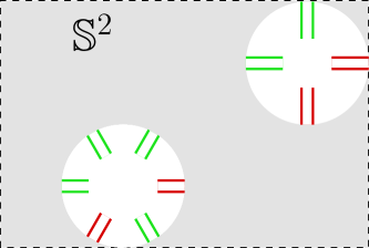
Figure 1. The gray part is an abstract representation of a multi-matrix model planar graph (after ‘vulcanizing’ the unbroken faces and forgetting everything but broken faces) with two faces broken by uncontracted half-edges. These boundaries determine the external leg structure decorating the cylinder (the two broken faces are interpreted as excised discs from $\mathbb{S}^{2}$ here). The 4-leg boundary in the upper right corner yields the cyclic word $ABBA$ (or $AABB$, or$\ldots$); the 6-legged one is $AABABA$ (or $AAABAB,\ldots$). The external leg structure is the disjoint union of these words.

Claim 2.1.

The external leg structure of the graph $\mathcal{G}$ given by (2.13) is $ABBA$, i.e.

Proof.

In $\mathcal{G}$ one has a single broken face (it can be recognized in the drawing (2.13) as the face that is unbounded). Starting at any point one reads off at the boundary of such face the word $ABBA$. One could also read off $BBAA$, $AABB$ or $BAAB$, depending on where one chooses to start. Yet, nothing changes, since the external leg structure is cyclic by definition. ∎

Claim 2.2.

The unique $($connected$\hskip 0.81pt)$ one-loop 1PI graph of order $b^{2}$ having a connected external leg structure is the graph $\mathcal{G}$ defined by (2.13).

In this statement the connectedness of the external leg structure means that $\mathcal{G}$ has a single broken face.

Proof.

By assumption, the graph has two interaction $ABAB$-vertices; let us name $V_{1}$ and $V_{2}$ the two copies. The 1PI-assumption constrains the $p$ propagators implied in the graph to $p>1$ (indeed, since the graph should be connected, and has two interaction vertices, a propagator should connect these. Should the graph have a single propagator, then removing it would yield a disconnected graph contradicting the 1PI assumption). On the other hand, the one-loop condition implies $p<3$ (if $p\geq 3$ then more loops are formed). Again, since the graph in question is 1PI, the $p=2$ propagators implied in the graph connect $V_{1}$ with $V_{2}$. If they connect two equal colors, we get a disconnected external leg structure, i.e. either the graph (2.12) or its $A\leftrightarrow B$ (i.e. green $\leftrightarrow$ red) version. Therefore, by assumption, the two propagators connecting $V_{1}$ with $V_{2}$ must have different color. The only such graph having also a connected external leg structure is $\mathcal{G}$ defined by (2.13). ∎

It is a Quantum Field Theory folklore result (see e.g. [16] and [17, Sec. 3.3]) that the effective action is the generating functional of 1PI graphs. Since neither the cyclicity of the vertices nor the coloring of thick edges has influence on the 1PI property, the effective action in multi-matrix models generates 1PI colored ribbon graphs; thus, that folklore result remains true in this setting. Further, the Functional Renormalization Equation governs the interpolating effective action, hence the 1PI condition is imposed from the outset. We have, in view of this:

Claim 2.3.

For the particular operator $-\frac{b}{2}\operatorname{Tr}(ABAB)$, a quadratic term $b^{2}$ in $\beta_{b}$ is not possible in Functional Renormalization $($in other words the coefficient of $b^{2}$ in $\beta_{b}$ vanishes, or in notation, $[b^{2}]\beta_{b}=0$$)$.

Proof.

Wetterich-Morris Equation imposes the one-loop structure on any non-linear term in the coupling constants (i.e.  on any non-vertex) appearing in each $\beta$-function. For the $\beta_{b}$-function, in particular, a second condition is that the external leg structure must be $ABAB$. These two conditions are mutually exclusive. Indeed, by Claim 2.2, the only such $\mathcal{O}(b^{2})$ graph is $\mathcal{G}$, which, by Claim 2.1, has an external leg structure $ABBA$.∎

Remark 2.4.

Some closely related, but not essential points:

• The correlation functions of matrix [13] and tensor field theories are indexed by boundary graphs [18]. The terminology makes sense graph theoretically but also geometrically in both the matrix and tensor field [14] contexts. In the case of matrix models, boundary graphs coincide with what we call here external leg structure. In matrix models, there are as many $\beta$-functions as correlation functions, hence the importance of the external leg structure. The map defined by ‘taking the boundary’ seems also to play a role in other renormalization theories, like Connes-Kreimer Hopf algebra approach [19]. In that theory for matrices (related construction appears in [20]) taking the boundary seems to be the residue map in terms of which one can define the coproduct of the Hopf algebra (also true [21] for the Ben Geloun-Rivasseau tensor field theory [22]).

• Other graphs might appear for real symmetric matrices, but the ribbons corresponding to Hermitian matrices remain untwisted, which played a role in the uniqueness of the graph above. It is not exaggerated to stress the reason for this rigidity, which is explained by the difference in the propagators of matrix models in ensembles $\{M\in M_{N}(\mathbb{K})\mid M^{\dagger}=M\}$ for different fields $\mathbb{K}$, i.e.

  $$\langle M_{ij}M_{kl}\rangle_{\mathbb{K}}=\frac{1}{N}\begin{cases}\displaystyle\frac{1}{2}\Big{(}\begin{array}[]{c}i\\[-5.0pt] j\end{array}\!\!\raisebox{-0.3pt}{\includegraphics[width=43.36464pt]{Listones/match}}\begin{array}[]{c}l\\[-5.0pt] k\end{array}+\begin{array}[]{c}i\\[-5.0pt] j\end{array}\!\!\raisebox{-0.3pt}{\includegraphics[width=43.36464pt]{Listones/mismatch}}\begin{array}[]{c}l\\[-5.0pt] k\end{array}\Big{)}&\mathbb{K}=\mathbb{R}\,\,(\text{symmetric real})\\[8.61108pt] \phantom{\displaystyle\frac{1}{2}\bigg{(}}\begin{array}[]{c}i\\[-5.0pt] j\end{array}\!\!\raisebox{-0.3pt}{\includegraphics[width=43.36464pt]{Listones/match}}\begin{array}[]{c}l\\[-5.0pt] k\end{array}&\mathbb{K}=\mathbb{C}\,\,(\text{Hermitian})\end{cases}$$ (2.14)

3. A proposal to obtain the Kazakov–Zinn-Justin phase diagram

We recall that in [1] the truncation is minimal. Thus, the running operators are also those in the bare action in eqs. (2.1a)-(2.1b).

In that truncation [1], if one computes correctly, $\beta_{b}\sim b$ (the value of the vertex); this is not wrong, but only says that such truncation threw away useful information. In order not to ‘waste’ the $b^{2}$ term, we propose to add the operator that captures it, so the new effective action reads:

$$\Gamma_{N}[A,B]=\frac{Z}{2}\operatorname{Tr}(A^{2}+B^{2})-\frac{\bar{a}}{4}\operatorname{Tr}(A^{4}+B^{4})-\frac{\bar{b}}{2}\operatorname{Tr}(ABAB)-\bar{c}\operatorname{Tr}(ABBA)\,,$$ (3.1)

where bar on quantities means unrenormalized and $Z$ is the (now common) wave function renormalization. The $ABBA$-operator also respects the original $\mathbb{Z}_{2}$-symmetries:

$$(A,B)\mapsto(B,A),\quad(A,B)\mapsto(-A,B)\,,\quad(A,B)\mapsto(A,-B)\,.$$ (3.2)

Now, $b^{2}$ does appear, but in the $\beta_{c}$-function. In fact $\beta_{c}\sim b^{2}+c^{2}+2ac$, ignoring the contribution ($\propto\,c$) of the vertex. This relation was obtained with the (‘coordinate-free’) method presented in [15, around Corollary 4.2]. Removing the symmetry condition ($g_{AAAA}=a=g_{BBBB}$) we initially imposed on the couplings for $A^{4}$ and $B^{4}$, and writing in full $g_{w}$ for the coupling of $\operatorname{Tr}\{w(A,B)\}$, being $w$ a cyclic word in $A,B$, one has

$$\qquad\qquad\beta{(g_{\color[rgb]{0,0.67,0}A\color[rgb]{0.84,0,0}BB\color[rgb]{0,0.67,0}A})}-g_{\color[rgb]{0,0.67,0}A\color[rgb]{0.84,0,0}BB\color[rgb]{0,0.67,0}A}(2\eta+1) \sim{g_{\color[rgb]{0,0.67,0}AAAA}\times g_{\color[rgb]{0,0.67,0}A\color[rgb]{0.84,0,0}BB\color[rgb]{0,0.67,0}A}}+g_{\color[rgb]{0.8,0,0}BBBB}\times g_{\color[rgb]{0,0.67,0}A\color[rgb]{0.84,0,0}BB\color[rgb]{0,0.67,0}A}$$

$$\!\qquad+(g_{\color[rgb]{0,0.67,0}A\color[rgb]{0.84,0,0}B\color[rgb]{0,0.67,0}A\color[rgb]{0.84,0,0}B})^{2}+{(g_{\color[rgb]{0,0.67,0}A\color[rgb]{0.84,0,0}BB\color[rgb]{0,0.67,0}A})^{2}}\,,$$ (3.3a)

obtained without the use of graphs. The missing coefficients (hidden in $$\sim \eta=-N\partial_{N}Z \beta$$ and implying the anomalous dimension ) are regulator-dependent and contain non-perturbative information, but the essential point is that now each -function has a transparent one-loop structure; to wit, the RHS of (3.3a) corresponds (respecting the order in that sum) with

$$\raisebox{-0.412pt}{\includegraphics[width=43.36464pt]{Listones/Feo_RibbonsA4_AABB90}}\,\,\,+\,\,\,\raisebox{-0.412pt}{\includegraphics[width=43.36464pt]{Listones/Feo_RibbonsB4_AABB90}}\,\,\,+\,\,\raisebox{-0.415pt}{\includegraphics[width=78.9218pt]{Listones/Feo_RibbonsABAB_ABAB90}}\,\,+\,\,\raisebox{-0.415pt}{\includegraphics[width=78.9218pt]{Listones/Feo_RibbonsAABB_AABB90}}\,$$ (3.3b)

It is also clear that the cyclic external leg structure of each of these terms is $ABBA$. Since it is easy to confuse the order of the letters, we stress that this is already an extended version of the $ABAB$-model to exemplify the one-loop structure of another coupling constant. But expressions (3.3) also give the (by Claim 2.2 unique) $\beta$-function where the $b^{2}$ actually has to sit.

Adding the $ABBA$ operator modifies the flow (for, now, $\beta_{b}-b(1+2\eta)\sim bc$) but in order to get the desired fixed points, higher-degree operators might still be required. As pointed out in the paragraph before [1, Sec. 3.3] when addressing higher-degree operators, $\operatorname{Tr}[(AB)^{3}]$ is indeed forbidden. However, there are degree-six operators that do preserve the symmetries (3.2), concretely $\operatorname{Tr}(ABABAA)$ or $\operatorname{Tr}(ABABBB)$, and contribute to the $\beta_{b}$-function (see [15, Thm. 7.2], where the RG-flow has been computed adding these operators), thus enriching the truncation.

Remark 3.1.

Some closing points one could learn from [1]:

• Notice that if we could somehow make $ABAB$ indistinguishable from $ABBA$, then the $\beta_{b}$-function [1, Eq. 3.41] would be, in that case, correct; see (2.3). This happens for a sub-ensemble of pairs of Hermitian matrices $A,B$ such that $AB$ is Hermitian (for then, $A$ and $B$ commute).

• Notice that the graph

    (3.4)

  would yield the $b^{2}$ term needed in [1, Eq. 3.41]. However, this graph is not possible, since the Ising operator $\sigma\operatorname{Tr}(AB)$, depicted with the bicolored bead and responsible for ‘changing color’, is not in the truncation behind that equation; moreover, if added, it violates two symmetries in (3.2), on top of $b^{2}$ being screened by $\sigma^{2}$ (that graph is a one-loop containing four operators: two Ising, two $ABAB$, alternated). Nevertheless, it seems plausible that the contamination of the running operators (i.e. considering operators that are not unitary invariant) might effectively lead to a color-change, as in (3.4).

4. Conclusion

We showed that the connection that [1] established between the Functional Renormalization Group (FRG) and a phase diagram—identified there with [2, Fig. 4]—relies on a $\beta$-function that does not have the one-loop structure of the Functional Renormalization Equation. In Section 3 above, we proposed to extend the minimalist truncation of [1] in order to find a FRG-compatible set of $\beta$-functions. Accomplishing this proposal would provide a sound bridge, in the intention of [1], between the FRG and Causal Dynamical Triangulations [23] through the $ABAB$-model [24, 25]. Finally, we provided in Remark 3.1 the condition one would need to add in order for the $\beta_{b}$-function given by [1, Eq. 3.41] to be correct.

References

- [1] A. Eichhorn, A.D. Pereira and A.G. Pithis, The phase diagram of the multi-matrix model with ABAB-interaction from functional renormalization, JHEP 20 (2020) 131 [2009.05111].
- [2] V.A. Kazakov and P. Zinn-Justin, Two matrix model with ABAB interaction, Nucl. Phys. B 546 (1999) 647 [hep-th/9808043].
- [3] H. Gies, Introduction to the functional RG and applications to gauge theories, Lect. Notes Phys. 852 (2012) 287 [hep-ph/0611146].
- [4] J. Berges, N. Tetradis and C. Wetterich, Nonperturbative renormalization flow in quantum field theory and statistical physics, Phys. Rept. 363 (2002) 223 [hep-ph/0005122].
- [5] C. Wetterich, Exact evolution equation for the effective potential, Phys. Lett. B 301 (1993) 90 [1710.05815].
- [6] T.R. Morris, The Exact renormalization group and approximate solutions, Int. J. Mod. Phys. A 9 (1994) 2411 [hep-ph/9308265].
- [7] G. ’t Hooft, A Planar Diagram Theory for Strong Interactions, Nucl. Phys. B72 (1974) 461.
- [8] J.E. Andersen, L.O. Chekhov, R.C. Penner, C.M. Reidys and P. Sułkowski, Topological recursion for chord diagrams, RNA complexes, and cells in moduli spaces, Nucl. Phys. B866 (2013) 414 [1205.0658].
- [9] J.E. Andersen, L.O. Chekhov, R. Penner, C.M. Reidys and P. Sulkowski, Enumeration of RNA complexes via random matrix theory, Biochem. Soc. Trans. 41 (2013) 652 [1303.1326].
- [10] E. Brezin, C. Itzykson, G. Parisi and J. Zuber, Planar Diagrams, Commun. Math. Phys. 59 (1978) 35.
- [11] R.C. Penner, Perturbative series and the moduli space of Riemann surfaces, J. Diff. Geom. 27 (1988) 35.
- [12] C.I. Pérez-Sánchez, Surgery in colored tensor models, J. Geom. Phys. 120 (2017) 262 [1608.00246].
- [13] H. Grosse and R. Wulkenhaar, Self-Dual Noncommutative -Theory in Four Dimensions is a Non-Perturbatively Solvable and Non-Trivial Quantum Field Theory, Commun. Math. Phys. 329 (2014) 1069 [1205.0465].
- [14] C.I. Pérez-Sánchez, The full Ward-Takahashi Identity for colored tensor models, Commun. Math. Phys. 358 (2018) 589 [1608.08134].
- [15] C.I. Pérez-Sánchez, On multimatrix models motivated by random Noncommutative Geometry I: the Functional Renormalization Group as a flow in the free algebra, Ann. Henri Poincaré (2021) [2007.10914].
- [16] R.E. Borcherds and A. Barnard, Lectures on Quantum Field Theory, math-ph/0204014.
- [17] A. Connes and M. Marcolli, Noncommutative Geometry, Quantum Fields and Motives, American Mathematical Society (2007).
- [18] V. Bonzom, R. Gurău, J.P. Ryan and A. Tanasă, The double scaling limit of random tensor models, JHEP 09 (2014) 051 [1404.7517].
- [19] A. Connes and D. Kreimer, Renormalization in quantum field theory and the Riemann-Hilbert problem. 1. The Hopf algebra structure of graphs and the main theorem, Commun. Math. Phys. 210 (2000) 249 [hep-th/9912092].
- [20] A. Tanasă and F. Vignes-Tourneret, Hopf algebra of non-commutative field theory, J. Noncommutat. Geom. 2 (2008) 125 [0707.4143].
- [21] M. Raasakka and A. Tanasă, Combinatorial Hopf algebra for the Ben Geloun-Rivasseau tensor field theory, Sem. Lothar. Combin. 70 (2014) B70d [1306.1022].
- [22] J. Ben Geloun and V. Rivasseau, A Renormalizable 4-Dimensional Tensor Field Theory, Commun. Math. Phys. 318 (2013) 69 [1111.4997].
- [23] J. Ambjørn, J. Jurkiewicz, R. Loll and G. Vernizzi, Lorentzian 3-D gravity with wormholes via matrix models, JHEP 09 (2001) 022 [hep-th/0106082].
- [24] J. Ambjørn, J. Jurkiewicz, R. Loll and G. Vernizzi, 3-D Lorentzian quantum gravity from the asymmetric ABAB matrix model, Acta Phys. Polon. B 34 (2003) 4667 [hep-th/0311072].
- [25] J. Ambjørn, J. Jurkiewicz and R. Loll, Renormalization of 3-d quantum gravity from matrix models, Phys. Lett. B 581 (2004) 255 [hep-th/0307263].