Highly efficient parallel grand canonical simulations of interstitial-driven deformation-diffusion processes

Abstract

Diffusion of interstitial alloying elements like H, O, C, and N in metals and their continuous relocation and interactions with their microstructures have crucial influences on metals’ properties. However, besides limitations in experimental tools in capturing these mechanisms, the inefficiency of numerical tools also inhibits modeling efforts. Here, we present an efficient framework to perform hybrid grand canonical Monte Carlo and molecular dynamics simulations that allow for parallel insertion/deletion of Monte Carlo moves. A new methodology for calculation of the energy difference at trial moves that can be applied to many-body potentials as well as pair ones is a primary feature of our implementation. We study H diffusion in Fe (ferrite phase) and Ni polycrystalline samples to demonstrate the efficiency and scalability of the algorithm and its application. The computational cost of using our framework for half a million atoms is a factor of 250 less than the cost of using existing libraries.

I Introduction

H-embrittlement, oxidation, creep, and carbide precipitation are examples of life-limiting chemo-mechanical mechanisms of metallic alloys in service. While continuum theories can capture the deformation mechanism phenomenologically, they have a limited range of validity when the inherent interactions between deformation and diffusion are unspecified. On the other hand, simulations at atomic resolution can reveal the underlying mechanisms and their correlations, but are severely limited in computational efficiency.

Molecular dynamics (MD) simulations have been widely used for equilibrium and non-equilibrium processes, while they have limitations in capturing long time-scale mechanisms such as diffusion. Monte Carlo (MC) simulations, besides their convenience in implementation, cannot capture non-equilibrium deformation mechanisms. The combination of these two techniques seems to be ideal. However, in practice, the probabilistic nature of the MC scheme and also the evolving number of degrees of freedom complicate the efficient implementation, i.e., parallelization of the hybrid MC-MD framework on multi-core architectures.

A parallelization scheme that can perform simultaneous MC moves based on domain decomposition was proposed by Sadigh et al. sadigh_scalable_2012 . Later on, Yamakov yamakov_parallel_2016 implemented parallel MD and semi-grand canonical Monte Carlo (SGCMC) simulations using this algorithm to model deformation-diffusion of substitutional alloys. Here, we present a newly developed software package that, among many features, has new hybrid grand canonical Monte Carlo (GCMC) and MD algorithms to model interstitial deformation-diffusion processes. In this package, GCMC, much like MD, is efficiently parallelized using domain decomposition. In addition, we introduce a more generalized concept of the linked list algorithm allen_computer_2017 that can be utilized to greatly improve the performance of the GCMC algorithm. Performing isothermal H-charging and discharging in a Ni model material will show that our library has two orders of magnitude less computational cost than LAMMPS plimpton_fast_1995 . Moreover, being able to conduct simulations at polycrystalline scale reveals the unknown parameters of analytic formulas to extract the concentration-pressure relationship of different microstructural defects in a model material system.

II Methodology

II.1 Theory

II.1.1 Proof of Detailed Balance

Consider a simulation supercell with a fixed total volume $V$, temperature $T$, and a chemical potential $\mu$ of an isotope of mass $m$. Even though the treatment here is for a monatomic system, it can be trivially generalized to multiple chemical species (isotopes), with constant $\{\mu_{c},m_{c}\}$ for $c=1\cdots C$ nuclide species. In the semi-classical treatment, the grand partition function $\mathcal{Q}$ can be written for $N$ identical particles of position vector ${\bf x}^{3N}\equiv{\bf x}_{1}{\bf x}_{2}...{\bf x}_{N}$ as follows kardar_statistical_2007 :

$$\mathcal{Q}\left(T,\mu,V\right)\equiv\sum_{N=0}^{\infty}\int\frac{d{\bf x}^{3N}}{N!\lambda_{\mathrm{th}}^{3N}}e^{\beta\left(N\mu-U\left(\mathbf{x}^{3N}\right)\right)},$$ (1)

where $\beta\equiv\left(k_{\mathrm{B}}T\right)^{-1}$, $\lambda_{\mathrm{th}}\equiv h/\sqrt{2\pi mk_{\mathrm{B}}T}$ is the thermal de Broglie wavelength, and $U\left(\mathbf{x}^{3N}\right)$ denotes the potential energy of the system. The differential probability of finding the system at a phase-space volume $\left(N,\mathbf{x}^{3N}\right)$ is therefore:

$$p\left(N,\mathbf{x}\right)d\mathbf{x}^{3N}=\frac{d\mathbf{x}^{3N}}{N!\lambda_{\mathrm{th}}^{3N}}e^{\beta\left(\mathcal{G}+\mu N-U\left(\mathbf{x}^{3N}\right)\right)},$$ (2)

where $\mathcal{G}\equiv-k_{\mathrm{B}}T\log\mathcal{Q}$ is the grand potential. Note that if we consider the particle-index permutation symmetry in ${\bf x}^{3N}\equiv{\bf x}_{1}{\bf x}_{2}...{\bf x}_{N}$, there are $N!$ copies of this phase-space volume with exactly the same $U$ and therefore the same probability density. (2) represents just one of these copies in a particular differential volume $d{\bf x}^{3N}=d{\bf x}_{1}d{\bf x}_{2}...d{\bf x}_{N}$, namely nuclide 1 in $({\bf x}_{1},{\bf x}_{1}+d{\bf x}_{1})$, nuclide 2 in $({\bf x}_{2},{\bf x}_{2}+d{\bf x}_{2})$, …, nuclide $N$ in $({\bf x}_{N},{\bf x}_{N}+d{\bf x}_{N})$.

Metropolis Monte Carlometropolis_equation_1953 relies on transition rates that respects Detailed Balance. If we perform particle insertion with some ${\rm transition}\left(N,\mathbf{x}^{3N}\rightarrow N+1,\mathbf{x}^{3N+3}\right)d\mathbf{x}^{3N+3}$ rate where the proportionality to destination volume $d\mathbf{x}^{3N+3}$ is made explicit, leaving the ${\rm transition}\left(N,\mathbf{x}^{3N}\rightarrow N+1,\mathbf{x}^{3N+3}\right)$ function itself an intensive quantity with finite value, then the corresponding reciprocal deletion rate must satisfy

$$\frac{{\rm transition}\left(N,\mathbf{x}^{3N}\rightarrow N+1,\mathbf{x}^{3N+3}\right)d\mathbf{x}^{3N+3}}{{\rm transition}\left(N+1,\mathbf{x}^{3N+3}\rightarrow N,\mathbf{x}^{3N}\right)d\mathbf{x}^{3N}}\;=\;\frac{p\left(N+1,\mathbf{x}^{3N+3}\right)d\mathbf{x}^{3N+3}}{p\left(N,\mathbf{x}^{3N}\right)d\mathbf{x}^{3N}},$$ (3)

where the right-hand side (RHS) is the ratio of the resident probabilities that we desire to approach, and the left-hand side (LHS) is the ratio of the conditional transition probabilities. It is then clear that differential phase-space volumes $d\mathbf{x}^{3N+3}$, $d\mathbf{x}^{3N}$ be cancelled out from both sides, making the exact values of these infinitesimal quantities immaterial, as they should be.

In principle, there needs to be no relation between $\mathbf{x}^{3N}$ and $\mathbf{x}^{3N+3}$; in other words, the positions of all atoms can be changed, even by a lot, in one move. But in the simplest incarnation that preserves Detailed Balance, we choose to preserve almost all of the atomic positions except for the atom (or a position) in question:

$$\mathbf{x}^{3N+3}\;=\;\mathbf{x}^{3N}{\bf x}_{\rm question}$$ (4)

in which case

$$d\mathbf{x}^{3N+3}\;=\;d\mathbf{x}^{3N}d{\bf x}_{\rm question},$$ (5)

and (3) is simplified to

$$\frac{{\rm transition}\left(N,\mathbf{x}^{3N}\rightarrow N+1,\mathbf{x}^{3N+3}\right)d{\bf x}_{\rm question}}{{\rm transition}\left(N+1,\mathbf{x}^{3N+3}\rightarrow N,\mathbf{x}^{3N}\right)}\;=\;\frac{e^{\beta\left(\mu-\Delta U\right)}d{\bf x}_{\rm question}}{(N+1)\lambda_{\mathrm{th}}^{3}}$$ (6)

where

$$\Delta U\;\equiv\;U\left(\mathbf{x}^{3N+3}\right)-U\left(\mathbf{x}^{3N}\right)$$ (7)

is always the energy difference between the high-particle-number configuration and the low-particle-number configuration.

There is an index permutation issue, though, about exactly what (6) means. We know there are $N!$ copies of a particular differential volume hypercube $d{\bf x}^{3N}=d{\bf x}_{1}d{\bf x}_{2}...d{\bf x}_{N}$ that are energetically degenerate, permuting only the position of indistinguishable atoms. Similarly, we know that $(N+1)!$ copies of the differential volume hypercube $d{\bf x}^{3N+3}=d{\bf x}_{1}d{\bf x}_{2}...d{\bf x}_{N+1}$. Are we allowing Monte Carlo transitions between any pair of them, i.e. a total of $N!(N+1)!$ transitions in labelled-atom space, or are we only adding/deleting the last atom in the labelled-atom space without random permutation afterwards, i.e. in total only $(N+1)N!=(N+1)!$ Monte Carlo transition bridges? Since with the same computational cost, building more Monte Carlo bridges facilitate approaching equilibrium, the first interpretation ($N!(N+1)!$ transitions) is preferable. Thus, if we take $\{N,\mathbf{x}^{3N}\}$ to mean the “index-free” collection of all $N!$ degenerate copies, where every copy in the $\{N,\mathbf{x}^{3N}\}$ set automatically share the weight in the collective, then (6) is simplified to

$$\frac{{\rm transition}\left(\{N,\mathbf{x}^{3N}\}\rightarrow\{N+1,\mathbf{x}^{3N+3}\}\right)d{\bf x}_{\rm question}}{{\rm transition}\left(\{N+1,\mathbf{x}^{3N+3}\}\rightarrow\{N,\mathbf{x}^{3N}\}\right)}\;=\;\frac{e^{\beta\left(\mu-\Delta U\right)}d{\bf x}_{\rm question}}{\lambda_{\mathrm{th}}^{3}},$$ (8)

where the $\{N,\mathbf{x}^{3N}\}$ notation is philosophically closer to the quantum mechanical interpretation for identical particles.

Requirement (8) is not that different from the standard Monte Carlo for the canonical ensemble. Given one is at $N,\mathbf{x}^{3N}$, one can attempt to insert (probability $a^{+}$) / accept insertion, or attempt to delete ($a^{-}=1-a^{+}$) / accept deletion (OKeeffeRO07 ). Both types of attempts would involve computational cost, and rejection of either type of attempts would mean wasted computations, and therefore $a^{+}/a^{-}$ may be chosen to optimize performance, i.e. speed of approaching chemical equilibrium, and efficiency in computing the thermodynamic averages of measurables.

Within the $a^{+}$ attempt branch, there is a question of where to insert. Again in the spirit of the simplest incarnation, we can choose “anywhere in the supercell, equally”, and therefore the attempt probability to $d{\bf x}_{\rm question}$ is $(a^{+}/V)d{\bf x}_{\rm question}$, representing a spatially uniform prior. It does not have to be this way. If we have advanced screening information, we could use umbrella sampling to tune this attempt probability (indeed, with the domain decomposition scheme to come later, such issue could arise). But right now let us choose the simplest insertion prior.

Within the $a^{-}$ attempt branch, we can also choose “any of the atoms in the supercell, equally”. It does not have to be this way. If we have advanced screening information, we could may umbrella sampling to tune this attempt probability also. But the $a^{-}/N$ prior (or $a^{-}/(N+1)$ for the high-particle-number configuration) does lead to the simplest proof of detailed balance. Therefore, with these simplest insertion/deletion priors, the requirement (8) is converted to

$$\frac{(a^{+}/V){\rm acceptance}\left(\{N,\mathbf{x}^{3N}\}\rightarrow\{N+1,\mathbf{x}^{3N+3}\}\right)}{(a^{-}/(N+1)){\rm acceptance}\left(\{N+1,\mathbf{x}^{3N+3}\}\rightarrow\{N,\mathbf{x}^{3N}\}\right)}\;=\;\frac{e^{\beta\left(\mu-\Delta U\right)}}{\lambda_{\mathrm{th}}^{3}},$$ (9)

where $d{\bf x}_{\rm question}$ is cancelled out, or

$$\frac{{\rm acceptance}\left(\{N,\mathbf{x}^{3N}\}\rightarrow\{N+1,\mathbf{x}^{3N+3}\}\right)}{{\rm acceptance}\left(\{N+1,\mathbf{x}^{3N+3}\}\rightarrow\{N,\mathbf{x}^{3N}\}\right)}\;=\;\frac{a^{-}Ve^{\beta\left(\mu-\Delta U\right)}}{a^{+}(N+1)\lambda_{\mathrm{th}}^{3}}.$$ (10)

The Metropolis Monte Carlo dichotomymetropolis_equation_1953 is then used to achieve (10) literally, by making one of the ${\rm acceptance}\left(\{N,\mathbf{x}^{3N}\}\rightarrow\{N+1,\mathbf{x}^{3N+3}\}\right)$, ${\rm acceptance}\left(\{N+1,\mathbf{x}^{3N+3}\}\rightarrow\{N,\mathbf{x}^{3N}\}\right)$ unity, and the other $\leq 1$, depending on the sign of the RHS. So the standard GCMC algorithm is just

$${\rm acceptance}\left(\{N,\mathbf{x}^{3N}\}\rightarrow\{N+1,\mathbf{x}^{3N+3}\}\right)\;=\;\left\{\begin{array}[]{cc}1,&\frac{a^{-}Ve^{\beta\left(\mu-\Delta U\right)}}{a^{+}(N+1)\lambda_{\mathrm{th}}^{3}}\geq 1,\\ \frac{a^{-}Ve^{\beta\left(\mu-\Delta U\right)}}{a^{+}(N+1)\lambda_{\mathrm{th}}^{3}},&\frac{a^{-}Ve^{\beta\left(\mu-\Delta U\right)}}{a^{+}(N+1)\lambda_{\mathrm{th}}^{3}}<1,\end{array}\right.$$ (11)

and

$${\rm acceptance}\left(\{N+1,\mathbf{x}^{3N+3}\}\rightarrow\{N,\mathbf{x}^{3N}\}\right)\;=\;\left\{\begin{array}[]{cc}1,&\frac{a^{+}(N+1)\lambda_{\mathrm{th}}^{3}}{a^{-}Ve^{\beta\left(\mu-\Delta U\right)}}\geq 1,\\ \frac{a^{+}(N+1)\lambda_{\mathrm{th}}^{3}}{a^{-}Ve^{\beta\left(\mu-\Delta U\right)}},&\frac{a^{+}(N+1)\lambda_{\mathrm{th}}^{3}}{a^{-}Ve^{\beta\left(\mu-\Delta U\right)}}<1,\end{array}\right.$$ (12)

or equivalently,

$${\rm acceptance}\left(\{N,\mathbf{x}^{3N}\}\rightarrow\{N-1,\mathbf{x}^{3N-3}\}\right)\;=\;\left\{\begin{array}[]{cc}1,&\frac{a^{+}N\lambda_{\mathrm{th}}^{3}}{a^{-}Ve^{\beta\left(\mu-\Delta U\right)}}\geq 1,\\ \frac{a^{+}N\lambda_{\mathrm{th}}^{3}}{a^{-}Ve^{\beta\left(\mu-\Delta U\right)}},&\frac{a^{+}N\lambda_{\mathrm{th}}^{3}}{a^{-}Ve^{\beta\left(\mu-\Delta U\right)}}<1,\end{array}\right.$$ (13)

where $\Delta U$ is always the energy difference between the high-particle-number configuration and the low-particle-number configuration. It is seen from above that $a^{+}/a^{-}$, $1/V$ and $1/N$ are just choices, reflecting the simplest prior about how to make moves. There is nothing set in stone about them. As long as we use these choices consistently, detailed balance can be established.

It is clear from the derivations above that the $0<a^{+}<1$ insertion attempt rate and $a^{-}=1-a^{+}$ deletion attempt rate can be arbitrarily tuned, and also the $(a^{+}/V)d{\bf x}_{\rm question}$ and $a^{-}/N$ priors can be substantially changed. Indeed, our domain decomposition scheme below changes these prefactors of Monte Carlo sampling for each domain, as $N_{\rm domain}/V_{\rm domain}$ can vary from domain to domain, and does not have to be equal to the average $N/V$.

II.1.2 Domain Decomposition

Imagine that our supercell is spatially partitioned into $d=1..D$ separate domains. Analytically, one can rearrange (1) into the following form

$$\mathcal{Q}\left(T,\mu,V\right)=\mathcal{I}_{1}\cdots\mathcal{I}_{D}\exp\left[-\beta U\left(\mathbf{x}^{3N_{1}},\cdots,\mathbf{x}^{3N_{d}}\right)\right],$$ (14)

where

$$\mathcal{I}_{d}\equiv\sum_{N_{d}=0}^{\infty}\int_{V_{d}}\frac{e^{\beta\mu N_{d}}}{N_{d}!\lambda_{\mathrm{th}}^{3N_{d}}}d\mathbf{x}^{3N_{d}},$$ (15)

is an integration and summation operator. The $1/N_{d}!$ prefactor comes from the combinatoric $N!/N_{1}!N_{2}!...N_{D}!$ copies of assigning labeled but identical nuclides to different domains, that yields the same integral for (1). Namely, in the way (1) was written, all particles can traverse and live in all domains, but now in the new form (14), within each $\mathcal{I}_{d}$ only “citizens” of that domain can live and contribute to the integral. Therefore the probability density of a microstate while ignoring the labeling of particles inside each domain is:

$$\mathrm{bar}{p}\left(\{N_{1},\mathbf{x}^{3N_{1}}\},\cdots,\{N_{D},\mathbf{x}^{3N_{D}}\}\right)=e^{\beta\mathcal{G}}\left(\prod_{d=1}^{D}\frac{d\mathbf{x}^{3N_{d}}}{\lambda_{\mathrm{th}}^{3N_{d}}}e^{\beta\mu N_{d}}\right)\exp\left[-\beta U\left(\mathbf{x}_{1},\cdots,\mathbf{x}_{D}\right)\right].$$ (16)

Now let us modify the standard GCMC algorithm by changing the priors. Every time that an insertion or deletion attempt trial is to be performed, one of the domains, say $d$ is randomly chosen with a probability $P_{d}$:

$$\sum_{N_{d}=0}^{\infty}P_{d}\;=\;1,$$ (17)

$P_{d}$ can be chosen to be proportional to its volume $V_{d}$, for example. Other priors may be chosen, but one should be careful in not letting $P_{d}$ depending on $N_{d}$, which can dynamically change, that unless proven, may break the detailed-balance requirement. A time-constant $\{P_{d}\}$ distribution should always be fine, if computational efficiency is of no concern.

The domain-$d$ insertion/deletion attempt rate is therefore $P_{d}a^{+}_{d}$ / $P_{d}a^{-}_{d}$, and we can straightforwardly show that

$${\rm acceptance}\left(\{N_{d},\mathbf{x}^{3N_{d}}\}\rightarrow\{N_{d}+1,\mathbf{x}^{3N_{d}+3}\}\right)\;=\;\left\{\begin{array}[]{cc}1,&\frac{a^{-}_{d}V_{d}e^{\beta\left(\mu-\Delta U\right)}}{a^{+}_{d}(N_{d}+1)\lambda_{\mathrm{th}}^{3}}\geq 1,\\ \frac{a^{-}_{d}V_{d}e^{\beta\left(\mu-\Delta U\right)}}{a^{+}_{d}(N_{d}+1)\lambda_{\mathrm{th}}^{3}},&\frac{a^{-}_{d}V_{d}e^{\beta\left(\mu-\Delta U\right)}}{a^{+}_{d}(N_{d}+1)\lambda_{\mathrm{th}}^{3}}<1,\end{array}\right.$$ (18)

and

$${\rm acceptance}\left(\{N_{d},\mathbf{x}^{3N_{d}}\}\rightarrow\{N_{d}-1,\mathbf{x}^{3N_{d}-3}\}\right)\;=\;\left\{\begin{array}[]{cc}1,&\frac{a^{+}_{d}N_{d}\lambda_{\mathrm{th}}^{3}}{a^{-}_{d}V_{d}e^{\beta\left(\mu-\Delta U\right)}}\geq 1,\\ \frac{a^{+}_{d}N\lambda_{\mathrm{th}}^{3}}{a^{-}_{d}V_{d}e^{\beta\left(\mu-\Delta U\right)}},&\frac{a^{+}_{d}N_{d}\lambda_{\mathrm{th}}^{3}}{a^{-}_{d}V_{d}e^{\beta\left(\mu-\Delta U\right)}}<1,\end{array}\right.$$ (19)

where $\Delta U$ is always the energy difference between the high-particle-number configuration and the low-particle-number configuration, and may depend on nearby domains, would preserve detailed balance. While (18),(19) is factually a different algorithm from (11),(13), their derivation follows exactly the same logic flow of the previous section, just with a different set of screening priors for making the next move. That is, in (18),(19) all “citizens” and all volume elements of the same “country” (domain) are treated the same before the “testing” (evaluation) of the potential (“presumed innocent”), but they are treated differently from country to country, whereas in (11),(13) all “citizens” and volume elements of the “world” (supercell) are treated equally before the testing of the potential. Even though (18),(19) is factually a different algorithm from (11),(13), as long as being run consistently, both can provide the equilibrium ensemble distribution (2). So in this sense, the domain partition of the supercell and the $\{P_{d},a^{+}_{d}/a^{-}_{d}\}$ are just “gauge” choices. These gauge choices, however, can be used to enhance the computational efficiency, because it is also clear from the logic flow of the proof that the “global citizen” approach of (11),(13) has no reason to posses optimal efficiency. Thus $\{V_{d},P_{d},a^{+}_{d}/a^{-}_{d}\}$ can be optimized, and when $V_{d}$ is taken to be quite small, it is clear that the $P_{d}$ spatial distribution would amount to a screening prior in umbrella sampling. While we do not explore this degree of freedom fully here in this paper, taking the simplest uniform $V_{d},P_{d}$ approach, the connection between domain decomposition and umbrella sampling is noted.

In addition to statistical sampling efficiency, there is the critical issue of efficient interatomic potential evaluation and load balancing, well-known in parallel computing for discrete agent-based simulations with short-range interactions. To this end, we break down a large supercell to smaller individual domains, whose size is chosen according to the radial cutoff distance in the interatomic potential and possible range of dynamic strain in the supercell Li05a ; Li05b . If the atoms in two separate domains cannot possibly interact with one another, energy difference would only depend on the affected domain and nothing prohibits us from performing $D$ simultaneous moves. Although the aforementioned assumption is almost never the case, it is possible to choose a pattern of domains such that the changes of potential energy due to any perturbation in the domains are independent of one another.

In the limit of truly isolated, non-interacting domains, it is clear that (14) will become a product of domain-specific grand partition functions. Thus, (18), (19) can be interpreted as running chemical equilibration between the constant-$\mu$ reservoir with each domain indepedently, using the classic GCMC algorithm. For load balancing purposes, the frequency of attempting to equilibrate these different domains may not need to be the same. In problems involving multi-phase chemical equilibrium, for instance, one may have a vapor phase with very different $N_{d}/V_{d}$ with a solid phase that it should be in equilibrium with. The freedom to pick $P_{d},a^{+}_{d}/a^{-}_{d}$ is in effect an umbrella-sampling scheme based on spatial location for load-balancing and sampling efficiency. For detailed balance, $P_{d},a^{+}_{d}/a^{-}_{d}$ should not depend on $N_{d}$ turn-by-turn, as $N_{d}$ sustains microscopic fluctuations. But by our derivations above, one should be able to re-adjust $P_{d},a^{+}_{d}/a^{-}_{d}$, say after every 1000 acceptances in that domain. One may also re-partition the supercell and redefine the domains for computational efficiency and expediency (say in a parallel computer, the number of allocated computing nodes may be forced to change from time to time), as long as this is not done too frequently.

II.2 Pattern selection algorithm

As mentioned in the previous section, it is possible to construct a pattern that involves non-interacting domains. Such a pattern can be established by considering that these domains have to be at least $n\times r_{\mathrm{C}}$ apart in any direction, where $r_{\mathrm{C}}$ is the cutoff radius of the interatomic potential and $n$ is an integer determined by the type of the forcefield (see sadigh_scalable_2012 ). For example, for pair potentials, $n=1$; for embedded atom method (EAM), $n=2$; and for modified EAM, $n=3$. Here, we describe how to construct such a pattern given that the domains are predetermined by the MD part of the GCMC+MD method.

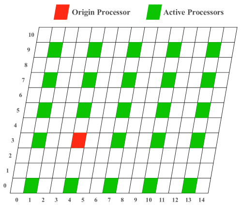
Figure 1: Schematic representation of subdomain selection pattern in two dimensions for $\vec{n}=\{15,11\}$ and $\vec{m}=\{2,1\}$. Red and green subdomains denote origin and active processors, respectively.

Suppose that our supercell is spanned by $n_{0}\times n_{1}\times n_{2}$ processors. Each processor controls a domain determined by a domain decomposition method. Fig. 1 depicts a simplified two dimensional schematic of such a supercell. Our first task is to determine how far apart our active domains should be. In other words, we must determine how many domains in each direction will at least cover $n\times r_{\mathrm{C}}$, namely integer vector $\vec{m}$. The best case scenario would be $\vec{m}=\{1,1,1\}$. In Fig. 1, $\vec{m}=\{2,1\}$. Let us define another integer vector

$$s_{i}=\lfloor n_{i}/\left(m_{i}+1\right)\rfloor,\quad i=0,1,2,$$ (20)

where $\lfloor.\rfloor$ is the floor function. $\vec{s}$ defines the number of simultaneous trial moves in each direction at any given GCMC step. Therefore, the total number of simultaneous trial moves is $s_{0}\times s_{1}\times s_{2}$.

At every step of GCMC, a processor is chosen at random. This processor will serve as the “origin,” and its position in the domain grid is denoted by an integer vector $\vec{o}$ (red domain in Fig. 1). Now, all the processors that perform trial moves, namely “active,” have to be determined (green domains in Fig. 1).

Consider a processor whose position in the domain grid is denoted by the integer vector $\vec{p}$. This processor is active if and only if

$$\sum_{i=0}^{2}\left[\left(p_{i}+n_{i}-o_{i}\right)\mathrm{mod}\,n_{i}\right]\mathrm{mod}\left(m_{i}+1\right)=0$$ (21)

where “$\mathrm{mod}$” denotes a modulo operation. The first modulo operation takes into account the periodic boundary condition. The second one ensures that active domains are non-interacting. Once the active processors are determined, they will perform trial moves simultaneously.

II.3 Potential energy difference calculation

As was pointed out earlier, the most expensive part of GCMC or any kind of atomistic simulation is the potential energy evaluation. This is due to the fact that potential energy and forces depend on the interaction of atoms. However, in the case of short-range force fields, the interactions of an atom with its surrounding can be restricted to a volume within a cutoff radius. In MD, all the pairs that are within a specified cutoff radius are included in a sparse matrix, usually referred to as a neighborlist. The forcefield employs the neighborlist to calculate energy/forces of the system. Since the generation of the neighborlist is itself time-consuming, researchers have come up with two major algorithms to speed things up: the cell/linked list allen_computer_2017 and the Verlet algorithm verlet_computer_1967 .

The cell/linked list algorithm is employed to limit the search volume for finding all the pairs interacting with an atom. The Verlet algorithm makes it possible to generate neighborlists less often.

In the case of GCMC, due to insertion or deletion moves, the maintenance of a neighborlist has extra complication. Nonetheless, a properly designed linked list will be relatively simple to update. In our implementation of parallel GCMC, every processor has its own linked list. Whenever a trial move is to be performed, a neighborlist for the affected atom will be instantly generated using the linked list and passed to the forcefield to calculate the energy difference. Next, the energy difference will determine whether the move is accepted or rejected. If the move is accepted, the linked list will be updated, accordingly.

In order to speed up even further, we modified the linked list algorithm. In the traditional linked list algorithm, the supercell is gridded by cubes (cells) with an edge of length $r_{\mathrm{C}}$. A linked list would be generated to link all the atoms within a cell. The basic premise of the algorithm is that when the neighborlist of an atom inside one of these cells is to be generated, only the atoms in the surrounding cells need to be searched, and these are accessible via the said linked list. In three dimensions, the search volume will be decreased from the volume of the whole supercell $V$ to $27r_{\mathrm{C}}^{3}$.

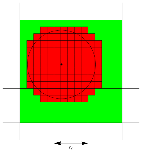
Figure 2: Classical linked list algorithm (green) versus proposed extension (red).

It is possible to reduce the search volume even further. In our implementation the cell’s edge length is $r_{\mathrm{C}}/m$, where $m$ is a positive integer to be set by the user, see Fig. 2. For two cells to interact, the minimum possible distance between them must be smaller than or equal to $r_{\mathrm{C}}$. Suppose cell $\Omega_{i}$ is labeled by a 3D vector $\vec{s}_{i}$, which determines its position in the grid and the volume it covers. In other words, $\vec{x}\in\Omega_{i}$ if

$$s_{i_{\alpha}}\frac{r_{\mathrm{C}}}{m}\leq x_{\alpha}<\left(s_{i_{\alpha}}+1\right)\frac{r_{\mathrm{C}}}{m},\quad\alpha=0,1,2.$$ (22)

One can easily show that for cells $\Omega_{i}$ and $\Omega_{j}$ to be interacting, the following must be true:

$$\sum_{\alpha=0}^{2}\left[\min\left(|s_{i_{\alpha}}-s_{j_{\alpha}}|-1,0\right)\right]^{2}\leq m^{2}.$$ (23)

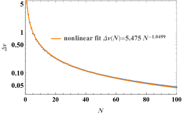
Figure 3: Relative excess search volume ($\Delta v$) with respect to number of discretization of cutoff radius ($N$).

Using this relationship, a “relative” neighborlist for the cells is created and will be utilized to build the neighborlist of a specific atom in one of the cells. Fig. 3 shows relative excess volume $\Delta v$ vs. the number of cutoff discretizations. Here, relative excess volume is defined by the ratio of search volume to the volume of the sphere with a radius $r_{\mathrm{C}}$ minus one. As the number of discretizations tends to infinity, the excess volume will tend to zero. One might naively conclude that the higher number of discretizations must inevitably lead to better performance. However, this improving trend is true only up to a point. The downside of increasing the number of discretizations is an increase in the memory storage of the head array of the linked list. If the storage becomes too large, it can lead to cache pollution and indeed poor performance. Much like the Verlet algorithm, in which the size of the shell must be chosen according to the problem under study, the number of discretizations can be chosen empirically by trial and error.

III Results

III.1 Scalability tests

To demonstrate the performance and the scalability of our implementation, several benchmark simulations were performed. All of these tests were conducted on a Beowulf Linux cluster, where each of the computational nodes contained two Intel Xeon Gold 6248 processors with 20 cores. The code was compiled using a C++ GNU compiler and -O3 optimization flag.

These benchmarks simulated H absorption in a ferrite-phase Fe single crystal. A sample consisting of $64\times 64\times 64$ Fe body-centered-cubic unit cells was generated. To facilitate the insertion of H, $0.1\%$ of atoms were randomly removed. The total number of Fe (ferrite phase) atoms is approximately 524,000. The EAM interatomic potential developed by Ramasubramaniam et al. ramasubramaniam_interatomic_2009 was used to model atomic interactions.

The sample was in equilibrium with a reservoir that had a $-2.4242~{}\mathrm{eV}$ H chemical potential. The temperature was $300~{}\mathrm{K}$; in total, $10^{6}$ Monte Carlo insertion/deletion trials were conducted.

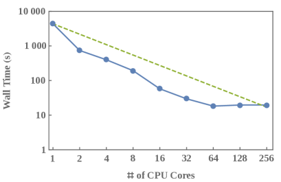
Figure 4: Total wall time as function of number of processors for $10^{6}$ MC trial moves of H in ferrite.

The tests were performed on 1, 2, 4, 8, 16, 32, 64, 128, and 256 CPU cores. For each given number of processors, 4 tests were performed, and the average wall time was recorded as the result. Fig. 4 shows the total CPU wall-time with respect to the number of processors, with the green dashed line being the ideal scalability line. Overall, the trend looks like a typical domain decomposition parallel application.

The biggest decrease in the computational time is the transition from the serial execution (1 core) to the parallel execution on 2 cores. However, this decrease is not due to parallel MC moves. In fact, the parallel MC moves will only take place starting from 16 processors. The main reason for the reduction in the computational time below the 16 cores is the reduction of cache pollution. In other words, due to the reduction of the number of atoms per processor, fewer cache misses would occur in the energy calculation.

The second largest drop takes place on transitioning from 8 to 16 processors, i.e., the onset of parallel MC moves. The improvement in computational time continues in a consistent manner up to 64 processors, reaching the start of a plateau. Increasing the number of processors does not enhance the performance any further. In fact, it is evident from the plot that the performance even slightly suffers. This slight decrease in performance can be explained by the overhead in inter-processor communication, which is the bottleneck of performance beyond this point. In total, in comparison to current widely used numerical libraries like LAMMPS plimpton_fast_1995 , for this problem, our framework is 250 times faster.

III.2 Isothermal H absorption/desorption in a Ni polycrystalline sample with free surfaces

As an example of application of the code, we chose isothermal H absorption/desorption in a polycrystalline Ni sample with free surfaces . This example was used in a previous work to study the mobility of dislocations due to H charging koyama_origin_2020 .

The sample has dimensions of 15 $\times$ 15 $\times$ 15 n m ³ and is periodic in the $x$ and $y$ directions. A 2.5 n m  vacuum layer was considered in the $z$ direction. The sample contains about 300,000 atoms in eight randomly oriented grains, which are approximately 7.5 n m  in diameter (see Fig. 5). For Ni and Ni-H interatomic interactions, the EAM potential angelo_trapping_1995 was adapted. Prior to absorption, the Nosé-Hoover thermostat was used to maintain the $NPT$ ensemble at room temperature $T$ = 300 K  and zero stress. After stress relaxation, the sample was relaxed in a $\mu VT$ ensemble using hybrid GCMC+MD for $2~{}\mathrm{n}\mathrm{s}$ with a time step of $0.5~{}\mathrm{f}\mathrm{s}$. The chemical potential of H was set to $\mu_{0}=-2.547~{}\mathrm{eV}$. After every 1000 steps of MD, 10,000 GCMC trials were conducted. Thereafter, H chemical potential was varied from $\mu_{0}$ to $\mu_{1}=-2.447~{}\mathrm{eV}$ in 50 increments of equal pressure change $(P_{1}-P_{0})/50$ from $P_{0}\propto\exp(2\mu_{0}/(k_{\mathrm{B}}T))$ to $P_{1}\propto\exp(2\mu_{1}/(k_{\mathrm{B}}T))$. At each increment, hybrid GCMC+MD was conducted for $200~{}\mathrm{p}\mathrm{s}$, using the scheme described above. After the chemical potential reached $\mu_{1}$, the procedure was reversed to return to the initial chemical potential. Fig. 6 and Fig. 7 show the evolution of the H-concentration in the bulk and the free surface of the polycrystalline Ni. No hysteresis was observed in either case. In the case of bulk atoms, H mainly locates in grain boundaries. As demonstrated, H concentration inside the bulk has a square root relation with pressure and obeys Sieverts’ law (see Supplementary Discussion 1 for the derivation of the equation).

However, for the surface, the story is different. Due to the high concentration of H on the surfaces, the ideal solution model with no H-H interactions, i.e., the basis of Sieverts’ law, is no longer valid. However, employing the regular solution model for 2D, i.e. the Fowler-Guggenheim adsorption isotherm model with lateral interaction between H* and H*, where * means surface site, can capture the behavior. We can define species $\mathrm{A}$ and $\mathrm{B}$ of regular solution as a surface site being occupied by H and a vacancy, respectively. The excess Gibbs free energy per site due to mixing is:

$$\Delta g\left(x\right)= n_{\mathrm{s}}k_{\mathrm{B}}T\left[\frac{x}{n_{\mathrm{s}}}\log\left(\frac{x}{n_{\mathrm{s}}}\right)+\left(1-\frac{x}{n_{\mathrm{s}}}\right)\log\left(1-\frac{x}{n_{\mathrm{s}}}\right)\right]$$

$$+n_{\mathrm{s}}w\frac{x}{n_{\mathrm{s}}}\left(1-\frac{x}{n_{\mathrm{s}}}\right).$$ (24)

Here $x$ and $n_{\mathrm{s}}$ denote the concentration of H and number of H sites per Ni atom, respectively. $w$ is the effective interaction energy of the regular model.

$$w=w_{\mathrm{AB}}-\frac{w_{\mathrm{AA}}+w_{\mathrm{BB}}}{2}$$ (25)

Therefore,

$$\mu_{\mathrm{H}}=\frac{\partial\Delta g}{\partial x}\Big{|}_{P,T}=k_{\mathrm{B}}T\log\left(\frac{x/n_{\mathrm{s}}}{1-x/n_{\mathrm{s}}}\right)+w\left(1-2\frac{x}{n_{\mathrm{s}}}\right),$$ (26)

As shown in details in Supplementary Discussion 1, since H is a diatomic gas, we can assume that its pressure is proportional to $\exp\left(2\beta\mu_{\mathrm{H}}\right)$, leading to

$$P_{\mathrm{H_{2}}}\left(x\right)=C\left(\frac{x/n_{\mathrm{s}}}{1-x/n_{\mathrm{s}}}\right)^{2}e^{-4\beta wx/n_{\mathrm{s}}}$$ (27)

Based on the concentration curves, we conclude that $n_{\mathrm{s}}=2$. Fig. 7 shows that the fit is in excellent agreement with the values obtained from the simulations. Based on our fitting, the effective interaction was calculated to be almost zero for H in grain boundaries (Langmuir–McLean isotherm), and $w=-0.22~{}\mathrm{eV}$ for H on free surfaces.

IV Discussion

In conclusion, we present a hybrid GCMC/MD framework that can efficiently simulate interstitial solid solution behavior in large polycrystalline samples. We show that the parallelization of the code is necessary for samples with large numbers of atoms .We provide two applied case studies for H-absorption/desorption in a polycrystalline Ni sample. Our analytical analysis was an excellent match with the obtained numerical results. The hidden parameters in the theory (H-interaction energy) can now be extracted from our efficient library. The framework has broad applications for simulation of interstitial alloying elements such as C, H, and O in different alloying systems and provides a new pathway to study the diffusion-deformation mechanisms in these samples.

All data required to reproduce the findings during this study are included in this Manuscript and Supplementary Information. The code is available for downloading at https://github.com/sinamoeini

V Acknowledgments

The authors acknowledge the financial support from Timken (to S.S.M.A.) and the Swiss National Science Foundation through Grant P300P2$\_$171423 (to S.M.T.M.) and the U.S. Department of Energy (DOE) Fuel Cell Technologies Office under award number DE-EE0008830 (to J.L.). Discussions with Doug Smith and R. Scott Hyde are gratefully appreciated. The simulations reported were performed on a local high-performance cluster. The authors also acknowledge the MIT SuperCloud and Lincoln Laboratory Supercomputing Center for providing (HPC and consultation) resources that have contributed to some of the numerical results reported within this paper.

VI Author Contributions

S.S.M.A. and J.L. designed the project. S.S.M.A., J.L. and S.M.T.M. performed the analytical derivations. S.S.M.A. wrote the code. S.S.M.A. and S.M.T.M. tested the code and ran the examples. S.S.M.A., S.M.T.M. and J.L. wrote the paper.

VII Competing Interests

The authors declare no competing interests.

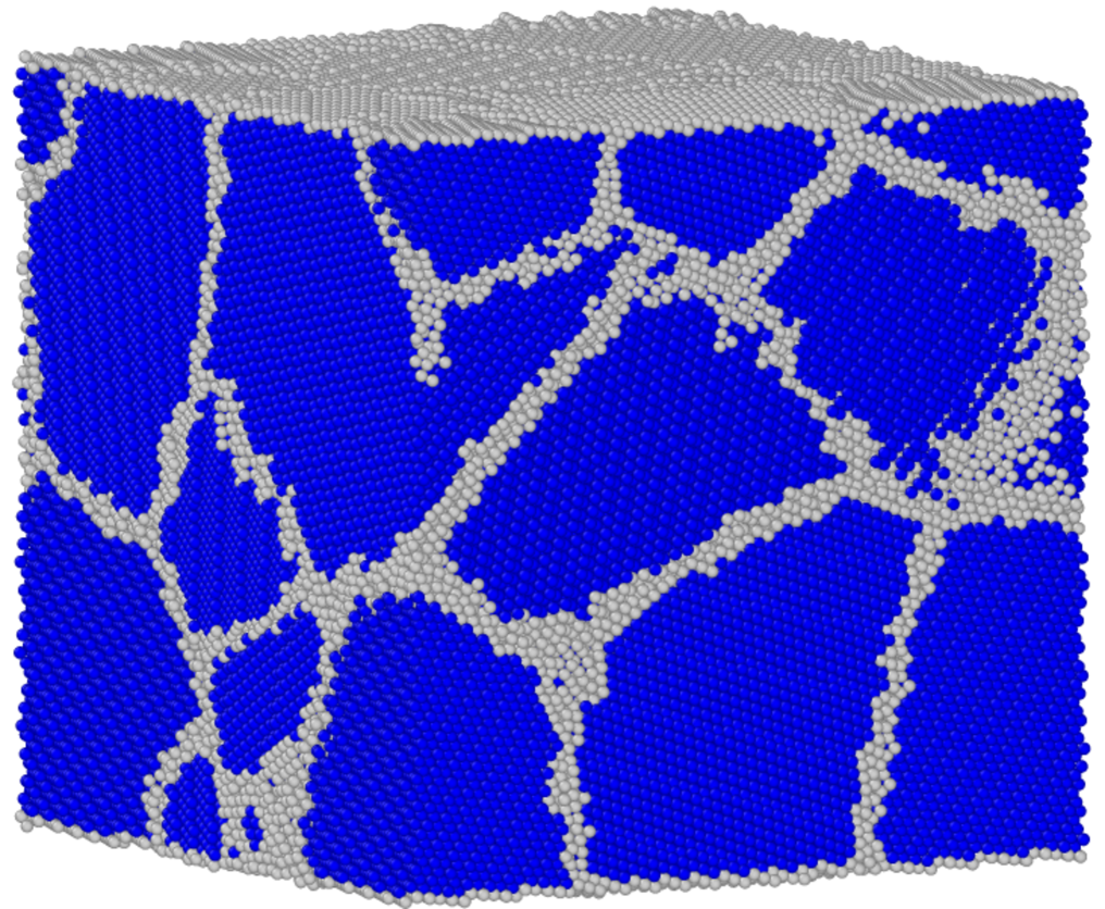
Figure 5: Polycrsytalline Ni sample with 8 randomly oriented grains for hybrid GCMC/MD simulations.

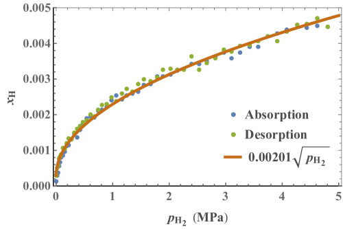
Figure 6: Isothermal curve for H absorption/desorption in the bulk of Ni polycrystalline sample. H concentration has a square root relationship with H pressure and follows Sieverts’ law. H mainly locates in grain boundaries.

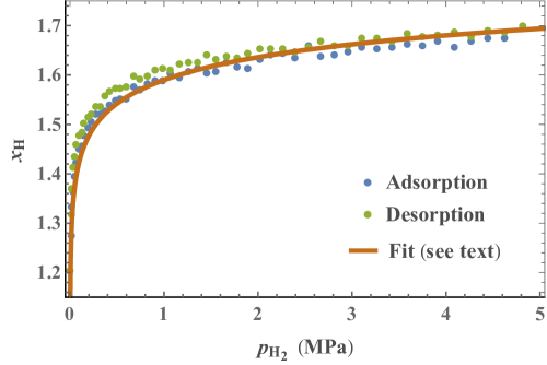
Figure 7: Isothermal curve for H absorption/desorption on the surface of Ni polycrystalline sample. H atom interactions influence the H concentration on the surface.

VIII Supplementary Information Document:

IX Supplementary Discussions 1— Analytical model of concentration-pressure relationships in Ni polycrystalline samples

Developing an analytical model for the relationship between a concentration and a pressure of H in different defects requires several steps of analysis. We started by developing the free energy of $\mathrm{H_{2}}$ molecules with the help of H diatomic partition functions. The derivative of the H free energy with respect to the volume and number of H defines the $P-\mu$ relationship. Next, we developed the Gibbs free energy of the polycrystalline bulk Ni sample by incorporating the enthalpy and entropy contributions of Ni, vacancy, and H atoms. The H concentration-chemical potential $x-\mu$ relationship will be obtained from this equation. Substitution of $\mu$ from the thermodynamic relationship establishes $x-P$. This is in fact Sieverts’ law which was used to fit the H concentration in grain boundaries. As discussed in the article, the mixing enthalpy term should also be considered for H on the surface of Ni polycrystalline samples; in this case H-H interactions due to the high concentration cannot be neglected. The following presents the details of our derivation.

IX.0.1 Partition function of H molecule ($\mathrm{H_{2}}$)

The partition function of H molecules consists of the partition functions contributed by H-H bonding and translational, vibrational, and rotational modes as follows:

$$z=z_{\mathrm{trans.}}z_{\mathrm{bond.}}z_{\mathrm{vib.}}z_{\mathrm{rot.}}$$ (28)

IX.0.2 Bonding

The H-H bonding partition function is

$$z_{\mathrm{bond.}}=e^{-\beta E_{\mathrm{b}}},$$ (29)

where $E_{\mathrm{b}}$ is the formation energy of the molecule at zero temperature, and $\beta$ is $(k_{\mathrm{B}}T)^{-1}$. Let us define a characteristic temperature as follows:

$$\Theta_{\mathrm{b}}=-\frac{E_{\mathrm{b}}}{k_{\mathrm{B}}}$$ (30)

Therefore

$$z_{\mathrm{bond.}}=\exp\left(\frac{\Theta_{\mathrm{b}}}{T}\right),$$ (31)

for H molecules

$$E_{\mathrm{b}}=-4.73832\mathrm{eV}\Rightarrow\Theta_{\mathrm{b}}=54985.9^{\circ}\mathrm{K}.$$ (32)

IX.0.3 Translational mode

Similar to the ideal gas

$$z_{\mathrm{trans.}}=\frac{V}{\lambda_{\mathrm{th}}^{3}},$$ (33)

where $V$ denotes the volume of the system and

$$\lambda_{\mathrm{th}}=\frac{h}{\sqrt{2\pi 2m_{\mathrm{H}}k_{\mathrm{B}}T}}.$$ (34)

Here, $h$, $k_{\mathrm{B}}$, $m_{\mathrm{H}}$, and $T$ are the Planck constant, Boltzmann constant, H atomic mass, and temperature, respectively. Please note that this $\lambda_{\mathrm{th}}$ differs from the one for H atoms by a factor of $2$ behind $m_{\mathrm{H}}$.

IX.0.4 Vibrational mode

The vibrational mode of diatomic gas must be dealt with from the perspective of a quantum harmonic oscillator.

$$z_{\mathrm{vib.}}=\sum_{n=0}^{\infty}e^{-\beta\hbar\omega\left(n+1/2\right)}=\frac{1}{2\sinh\left(\beta\hbar\omega/2\right)},$$ (35)

where

$$\hbar=\frac{h}{2\pi}.$$ (36)

To keep the notation consistent

$$z_{\mathrm{vib.}}=\frac{1}{2}\mathrm{cosech}\left(\frac{\beta h\omega}{4\pi}\right),$$ (37)

or even better we can write it as follows:

$$z_{\mathrm{vib.}}=\frac{1}{2}\mathrm{cosech}\left(\frac{\Theta_{\mathrm{v}}}{T}\right),$$ (38)

where

$$\Theta_{\mathrm{v}}=\frac{h\omega}{4\pi k_{\mathrm{B}}}.$$ (39)

For H molecules

$$\omega\approx 8.80803\times 10^{14}\mathrm{S^{-1}}\Rightarrow\Theta_{\mathrm{v}}=3363.89^{\circ}\mathrm{K}.$$ (40)

IX.0.5 Rotational mode

Like the vibrational mode, the rotational mode must also consider quantum mechanics.

$$z_{\mathrm{rot.}}=\sum_{l=0}^{\infty}\left(2l+1\right)\exp\biggl{[}-\frac{\hbar^{2}l\left(l+1\right)}{2Ik_{\mathrm{B}}T}\biggr{]}$$ (41)

At high temperature limits, the series can be calculated using the integration as:

$$z_{\mathrm{rot.}}\approx\frac{2Ik_{\mathrm{B}}T}{\hbar^{2}}.$$ (42)

However, at low temperatures, only the first two terms of the series are considered. Thus,

$$z_{\mathrm{rot.}}\approx\exp\biggl{[}-\frac{\hbar^{2}}{2Ik_{\mathrm{B}}T}\biggr{]}+3\exp\biggl{[}-\frac{2\hbar^{2}}{2Ik_{\mathrm{B}}T}\biggr{]}+\cdots.$$ (43)

Similarly to the vibrational mode, we can define a characteristic temperature as

$$\Theta_{\mathrm{r}}=\frac{h^{2}}{8\pi^{2}Ik_{\mathrm{B}}}.$$ (44)

For H,

$$I=2.84373\times 10^{-29}\mathrm{eVS^{2}}\Rightarrow=\Theta_{\mathrm{r}}=88.3977^{\circ}\mathrm{K}.$$ (45)

Since $\Theta_{\mathrm{r}}$ is much lower than the room temperature, for our purpose, the high temperature limit is more appropriate.

Finally, we can write the partition function of H molecules as follows:

$$z= V\mathrm{bar}{z}\left(T\right),$$ (46)

$$\mathrm{bar}{z}_{q}\left(T\right)= \frac{\sqrt{2}}{\lambda_{\mathrm{th}}^{3}}\exp\left(\frac{\Theta_{\mathrm{b}}}{T}\right)\frac{T}{\Theta_{\mathrm{r}}}\mathrm{cosech}\left(\frac{\Theta_{\mathrm{v}}}{T}\right),$$ (47)

$$\mathrm{bar}{z}_{c}\left(T\right)= \frac{\sqrt{2}}{\lambda_{\mathrm{th}}^{3}}\exp\left(\frac{\Theta_{\mathrm{b}}}{T}\right)\frac{T^{2}}{\Theta_{\mathrm{r}}\Theta_{\mathrm{v}}},$$ (48)

where

$$\mathrm{bar}{z}\left(T\right)= \frac{T^{3/2}}{\mathrm{bar}{\lambda_{\mathrm{th}}}^{3}}\exp\left(\frac{\Theta_{\mathrm{b}}}{T}\right)\frac{1}{2}\mathrm{cosech}\left(\frac{\Theta_{\mathrm{v}}}{T}\right)\frac{T}{\Theta_{\mathrm{r}}},$$ (49)

and

$$\mathrm{bar}{\lambda_{\mathrm{th}}}= 12.2961\mathrm{\AA}\sqrt{{}^{\circ}\mathrm{K}},$$

$$\Theta_{\mathrm{b}}= 54985.9^{\circ}\mathrm{K},$$

$$\Theta_{\mathrm{v}}= 3363.89^{\circ}\mathrm{K},$$

and

$$\Theta_{\mathrm{r}}= 88.3977^{\circ}\mathrm{K}.$$

IX.0.6 Free energy of $\mathrm{H_{2}}$ molecules

For $\mathrm{H_{2}}$ gas consisting of N molecules, the free energy density is as follows:

$$F =-Nk_{\mathrm{B}}T\log\left(\frac{V\mathrm{bar}{z}\left(T\right)}{N}\right)-Nk_{\mathrm{B}}T,$$ (50)

$$p_{\mathrm{H_{2}}} =-\frac{\partial F}{\partial V}\bigg{|}_{T,N}=nk_{\mathrm{B}}T,$$ (51)

$$S_{\mathrm{H_{2}}} =-\frac{\partial F}{\partial T}\bigg{|}_{V,N}=Nk_{\mathrm{B}}\biggl{[}1-\log\left(n\right)+\frac{\partial}{\partial T}T\log\mathrm{bar}{z}\left(T\right)\biggr{]},$$ (52)

$$\mu_{\mathrm{H_{2}}} =\frac{\partial F}{\partial N}\bigg{|}_{T,V}=-k_{\mathrm{B}}T\log\left(\frac{\mathrm{bar}{z}\left(T\right)}{n}\right),$$ (53)

where

$$n=\frac{N}{V}.$$ (54)

IX.0.7 Pressure-chemical potential ($P-\mu$) relationship

Let us express everything in terms of pressure to extract the ($P-\mu$) relationship as:

$$\frac{\mu_{\mathrm{H}}}{k_{\mathrm{B}}T} =-\frac{1}{2}\log\left(\frac{k_{\mathrm{B}}T\mathrm{bar}{z}\left(T\right)}{p_{\mathrm{H_{2}}}}\right).$$ (55)

IX.0.8 Free energy for a hydrogenated Ni polycrystalline sample

Considering $n_{\mathrm{s}}$ as the number of possible H sites per Ni atom and $x$ as the H concentration $x=N_{\mathrm{H}}/N_{\mathrm{Ni}}$, the free energy of the hydrogenated sample is:

$$F=Nf_{\mathrm{Ni}}+xN\Delta u_{\mathrm{H}}+n_{\mathrm{s}}Nk_{\mathrm{B}}T[\frac{x}{n_{\mathrm{s}}}\ln(\frac{x}{n_{\mathrm{s}}})+(1-\frac{x}{n_{\mathrm{s}}})\ln(1-\frac{x}{n_{\mathrm{s}}})],$$ (56)

where $f_{\mathrm{Ni}}$ and $\Delta u_{\mathrm{H}}$ are Ni and H enthalpy, respectively. To calculate $\mu_{\mathrm{H}}$, a partial derivative with respect to the number of H atoms $xN$ should be performed:

$$\mu_{\mathrm{H}}=\frac{\partial F}{\partial(xN)}=\frac{\partial F}{N\partial x}=\Delta u_{\mathrm{H}}+\frac{k_{\mathrm{B}}Tn_{\mathrm{s}}N}{N}[\frac{1}{n_{\mathrm{s}}}\ln(\frac{x}{n_{\mathrm{s}}})+\frac{\frac{1}{n_{\mathrm{s}}}\frac{x}{n_{\mathrm{s}}}}{\frac{x}{n_{\mathrm{s}}}}-\frac{1}{n_{\mathrm{s}}}\ln(1-\frac{x}{n_{\mathrm{s}}})-\frac{1}{n_{\mathrm{s}}}]$$ (57)

$$=\Delta u_{\mathrm{H}}+k_{\mathrm{B}}Tn_{\mathrm{s}}(\frac{1}{n_{\mathrm{s}}}(\ln(\frac{\frac{x}{n_{\mathrm{s}}}}{1-\frac{x}{n_{\mathrm{s}}}}))).$$

By substitution of $\mu$ with H pressure $P$ from Eq. 55, we have:

$$\frac{\mu_{\mathrm{H}}}{k_{\mathrm{B}}T}=\ln\sqrt{\frac{P_{\mathrm{H_{2}}}}{k_{\mathrm{B}}T\mathrm{bar}{z}(T)}}=\frac{\Delta u_{\mathrm{H}}}{k_{\mathrm{B}}T}+\ln(\frac{\frac{x}{n_{\mathrm{s}}}}{1-\frac{x}{n_{\mathrm{s}}}})).$$ (58)

IX.0.9 Sieverts’ law and H in grain boundaries

In the case of $(x\ll 1)$, which is the situation for H in grain boundaries, the above equation becomes more simplified as

$$\ln\frac{\sqrt{\frac{P_{\mathrm{H_{2}}}}{k_{\mathrm{B}}T\mathrm{bar}{z}(T)}}}{\frac{x}{n_{\mathrm{s}}}}=\frac{\Delta u_{\mathrm{H}}}{k_{\mathrm{B}}T}.$$ (59)

This is in fact Sieverts’ law, which shows that the H concentration $x$ is proportional to the square root of the pressure $P_{\mathrm{H_{2}}}$. This relationship is valid for the H in Ni grain boundaries.

$$x\propto A\sqrt{P_{\mathrm{H_{2}}}},$$ (60)

where A is a constant value. Fitting Sieverts’ law with our simulations, A is determined for the H in grain boundaries.

IX.0.10 H on free surfaces

Due to the high concentration of H atoms on the surfaces, the previous assumption of $x\ll 1$ is no longer valid. For this case, the H interactions should be also considered in the free energy. The interaction energy is as follows:

$$w=w_{\mathrm{AB}}-\frac{1}{2}(w_{\mathrm{AA}}+w_{\mathrm{BB}}),$$ (61)

where $\mathrm{A}$ denotes the interstitial sites filled with H, and $\mathrm{B}$ indicates vacant interstitial sites. Therefore, in this problem, only $w_{\mathrm{AA}}$ has a non-zero value. Extending Eq. 56 by considering this energy, the free energy of the free surfaces containing H atoms is:

$$F=Nf_{\mathrm{Ni}}+xN\Delta u_{\mathrm{H}}+n_{\mathrm{s}}Nk_{\mathrm{B}}T[\frac{x}{n_{\mathrm{s}}}\ln(\frac{x}{n_{\mathrm{s}}})+(1-\frac{x}{n_{\mathrm{s}}})\ln(1-\frac{x}{n_{\mathrm{s}}})]+n_{\mathrm{s}}N\frac{x}{n_{\mathrm{s}}}(1-\frac{x}{n_{\mathrm{s}}})w.$$ (62)

The derivative of the free energy with respect to the total number of H atoms has an additional term compared to the one for grain boundaries as follows:

$$\mu_{\mathrm{H}}=\frac{\partial F}{\partial(xN)}=\Delta u_{\mathrm{H}}+k_{\mathrm{B}}Tn_{\mathrm{s}}(\frac{1}{n_{\mathrm{s}}}(\ln(\frac{\frac{x}{n_{\mathrm{s}}}}{1-\frac{x}{n_{\mathrm{s}}}})))+(1-\frac{2x}{n_{\mathrm{s}}})w.$$ (63)

By substitution of $\mu_{\mathrm{H}}$ by the H pressure and simplification of this equation, we have:

$$CP_{\mathrm{H_{2}}}=(\frac{\frac{x}{n_{\mathrm{s}}}}{1-\frac{x}{n_{\mathrm{s}}}})^{2}e^{2(\frac{\Delta u_{\mathrm{H}}}{k_{\mathrm{B}}T}+(1-\frac{2x}{n_{\mathrm{s}}})\frac{w}{k_{\mathrm{B}}T})},$$ (64)

$$P_{\mathrm{H_{2}}}\left(x\right)=C\left(\frac{x/n_{\mathrm{s}}}{1-x/n_{\mathrm{s}}}\right)^{2}e^{-4\beta wx/n_{\mathrm{s}}},$$ (65)

where C is a constant. In the case of $w=0$, this equation transforms into Sieverts’ law.

References

- (1) Sadigh, B. et al. Scalable parallel Monte Carlo algorithm for atomistic simulations of precipitation in alloys. Physical Review B 85, 184203 (2012).
- (2) Yamakov, V. I. Parallel Grand Canonical Monte Carlo (ParaGrandMC) Simulation Code. Tech. Rep. (2016).
- (3) Allen, M. P. & Tildesley, D. J. Computer Simulation of Liquids (OUP Oxford, 2017), 2nd edn.
- (4) Plimpton, S. Fast Parallel Algorithms for Short-Range Molecular Dynamics. Journal of Computational Physics 117, 1–19 (1995).
- (5) Kardar, M. Statistical Physics of Particles (Cambridge University Press, 2007), 1st edn.
- (6) Metropolis, N., Rosenbluth, A. W., Rosenbluth, M. N., Teller, A. H. & Teller, E. Equation of State Calculations by Fast Computing Machines. The Journal of Chemical Physics 21, 1087–1092 (1953).
- (7) O’Keeffe, C., Ren, R. & Orkoulas, G. Spatial updating grand canonical monte carlo algorithms for fluid simulation: Generalization to continuous potentials and parallel implementation. J. Chem. Phys. 127, 194103 (2007).
- (8) Li, J. Basic molecular dynamics. In Yip, S. (ed.) Handbook of Materials Modeling, 565–588 (Springer, Dordrecht, 2005). Mistake free version at http://alum.mit.edu/www/liju99/Papers/05/Li05-2.8.pdf.
- (9) Li, J. Atomistic calculation of mechanical behavior. In Yip, S. (ed.) Handbook of Materials Modeling, 773–792 (Springer, Dordrecht, 2005). Mistake free version at http://alum.mit.edu/www/liju99/Papers/05/Li05-2.19.pdf.
- (10) Verlet, L. Computer ”Experiments” on Classical Fluids. I. Thermodynamical Properties of Lennard-Jones Molecules. Physical Review 159, 98–103 (1967).
- (11) Ramasubramaniam, A., Itakura, M. & Carter, E. A. Interatomic Potentials for Hydrogen in –Iron Based on Density Functional Theory. Phys. Rev. B 79, 174101 (2009).
- (12) Koyama, M. et al. Origin of micrometer-scale dislocation motion during hydrogen desorption. Science Advances 6, eaaz1187 (2020).
- (13) Angelo, J. E., Moody, N. R. & Baskes, M. I. Trapping of hydrogen to lattice defects in nickel. Modelling and Simulation in Materials Science and Engineering 3, 289 (1995).