Rotation-Equivariant Deep Learning
for Diffusion MRI

Abstract

Convolutional networks are successful, but they have recently been outperformed by new neural networks that are equivariant under rotations and translations. These new networks work better because they do not struggle with learning each possible orientation of each image feature separately. So far, they have been proposed for 2D and 3D data. Here we generalize them to 6D diffusion MRI data, ensuring joint equivariance under 3D roto-translations in image space and the matching 3D rotations in $q$-space, as dictated by the image formation. Such equivariant deep learning is appropriate for diffusion MRI, because microstructural and macrostructural features such as neural fibers can appear at many different orientations, and because even non-rotation-equivariant deep learning has so far been the best method for many diffusion MRI tasks. We validate our equivariant method on multiple-sclerosis lesion segmentation. Our proposed neural networks yield better results and require fewer scans for training compared to non-rotation-equivariant deep learning. They also inherit all the advantages of deep learning over classical diffusion MRI methods. Our implementation is available at https://github.com/philip-mueller/equivariant-deep-dmri and can be used off the shelf without understanding the mathematical background.

1 Introduction and Motivation

Diffusion MRI (dMRI) (Basser & Özarslan, 2009; Beaulieu, 2009) is an imaging technique capable of inferring properties of biological-tissue microstructure non-invasively. Each dMRI scan consists of multiple images taken with different diffusion gradients. It can be interpreted as 6D data where a coordinate (i.e. voxel location) in the 3D space of physical positions (called $p$-space in our work; sometimes also called $x$-space or $(x,y,z)$-space) and a coordinate in 3D diffusion-encoding space ($q$-space) are mapped to a signal intensity measured for that 6D coordinate. Note that while $p$-space is discretized to a finite Cartesian 3D grid described by the voxels of the scan, the $q$-space sampling scheme is typically not a regular grid.

Deep learning (Georgevici & Terblanche, 2019; LeCun et al., 2015; Goodfellow et al., 2016) proved highly beneficial for dMRI (Golkov et al., 2016a). It is a machine-learning technique to map input features to outputs. This mapping is done in several steps called layers. Each layer can separate or recombine low-level features to produce more abstract high-level features. Layers may contain learnable parameters. All layers are optimized jointly using a training dataset. Thus, unlike non-learnable processing pipelines, where useful information may be discarded partially in intermediate steps, deep learning can be trained in an end-to-end manner such that all processing steps are optimized to work well together and to serve the final goal.

Convolutional neural networks (CNNs) (LeCun et al., 2015; Goodfellow et al., 2016) restrict the learned mappings to be translation-equivariant and respect locality, meaning that features are detected equally well regardless of their translation (position) and regardless of what features are present far away in the image. These guaranteed properties of feature extraction are appropriate for many applications, including medical imaging, and improve the quality of results. This explains the success of CNNs in these applications. If rotation-equivariance (i.e. detecting features well, regardless of their rotational orientation) is appropriate as well, restricting the mappings further to be translation- and rotation-equivariant improves the quality of results even more, as was shown for 2D (Cohen & Welling, 2016; Worrall et al., 2016; Cohen & Welling, 2017; Weiler et al., 2018a) and 3D (Winkels & Cohen, 2018; Weiler et al., 2018b; Thomas et al., 2018; Worrall & Brostow, 2018; Esteves et al., 2018; Cohen et al., 2018; Anderson et al., 2019) data. Equivariance is formally defined in Appendix A.1.

In dMRI, rotation- and translation-equivariant deep learning is appropriate because features in the image (for example properties of neural fibers) should be detected equally well regardless of their position and orientation. A rotation and translation of an object or its parts/features in the scanner affects the image via the corresponding joint rotation in $p$- and $q$-space and the corresponding translation in $p$-space (see e.g. Definition 2 by Duits & Franken (2011)). Therefore, deep learning for dMRI should be equivariant under joint rotations in $p$- and $q$-space, and under translations in $p$-space. This guarantees that the position and orientation of the object and its parts in the scanner accordingly affects the position and orientation of the neural network output (if it has spatial dimensions), but does not affect other properties of the output, i.e. does not make the network output less correct.

Our contributions are the following:

• proposal of a neural network layer for 6D dMRI data respecting the equivariance properties of $p$- and $q$-space (i.e. adaptation of Thomas et al. (2018) and Weiler et al. (2018b) from 3D data to 6D dMRI data), including proofs of equivariance,

• efficient implementation of the proposed layer respecting the sampling properties of $p$- and $q$-space,

• experiments using our equivariant neural networks on a dMRI dataset for segmentation of multiple sclerosis lesions, demonstrating that our methods outperform existing methods and require less training data.

2 Related Work

Equivariant Deep Learning

In the last few years there has been much effort on developing neural networks that are equivariant under the group $\mathrm{SO}(3)$ of rotations or the group $\mathrm{SE}(3)$ of roto-translations. Several approaches use so-called irreducible representations of $\mathrm{SO}(3)$ and spherical harmonics to achieve full $\mathrm{SO}(3)$- or $\mathrm{SE}(3)$-equivariance for voxel data (Weiler et al., 2018b), for point clouds (Kondor, 2018; Thomas et al., 2018; Anderson et al., 2019), or for spherical signals (Cohen et al., 2017; Esteves et al., 2018; Cohen et al., 2018; Kondor et al., 2018). While these approaches use the same mathematical framework for achieving equivariance as used in the present work, they all only consider a single 3D space, whereas the present work extends these approaches to consider two linked 3D spaces at the same time, namely physical space and $q$-space. Methods using so-called regular representations (Winkels & Cohen, 2018; Worrall & Brostow, 2018) instead of irreducible representations are only suitable for discrete groups (Weiler et al., 2018b), so $\mathrm{SO}(3)$- or $\mathrm{SE}(3)$-equivariance can only be achieved approximately, by using discrete subgroups of $\mathrm{SO}(3)$ or $\mathrm{SE}(3)$.

For the 2D case, there are also prior works using irreducible representations like Worrall et al. (2016) (the 2D-equivalent to Weiler et al. (2018b)), Cohen & Welling (2017), or Weiler et al. (2018a).

In Weiler & Cesa (2019) a comparison of methods for the Euclidean group $\mathrm{E}(2)$ and its subgroups (including $\mathrm{SE}(2)$ and $\mathrm{SO}(2)$) is presented, and Della Libera et al. (2019) provide a comprehensive overview of approaches for $\mathrm{SE}(2)$, $\mathrm{SO}(2)$, $\mathrm{SE}(3)$, and $\mathrm{SO}(3)$.

Besides these approaches considering rotations, there are also more general methods for homogeneous spaces (Kondor & Trivedi, 2018; Cohen et al., 2019a), general manifolds (Cohen et al., 2019b; Bekkers, 2019), and for discrete groups (Cohen & Welling, 2016; Ravanbakhsh et al., 2017).

Deep Learning for Diffusion MRI

Deep learning is highly beneficial for dMRI. By avoiding suboptimal processing steps, it improves the results and allows to reduce the scan time by a factor of twelve (Ye et al., 2019). So far, it has used translation-equivariance (by using CNNs), but no rotation-equivariance. CNNs rely on the network learning rotation-equivariance during training, e.g. by assuming that the training dataset already demonstrates that different orientations of features have the same meaning or using data augmentation. However, it was shown for 2D (Cohen & Welling, 2016; Worrall et al., 2016; Cohen & Welling, 2017) and 3D (Weiler et al., 2018b; Thomas et al., 2018; Winkels & Cohen, 2018; Anderson et al., 2019; Worrall & Brostow, 2018; Cohen et al., 2018) data (and here we show for 6D dMRI data) that neural networks that guarantee rotation-equivariance yield better results than neural networks that need to go through a difficult learning process to achieve imperfect equivariance.

Machine learning for dMRI has also been successfully used beyond the usual supervised setting, namely for weakly-supervised localization (Golkov et al., 2018a), novelty detection (Golkov et al., 2016b; 2018b; Vasilev et al., 2020), and similar scenarios (Swazinna et al., 2019), i.e. detecting diseased voxels without the need for voxel-level training labels.

Apart from the named end-to-end approaches, there are also works that only replace parts of the classical processing pipeline for dMRI by deep learning. Some methods replace the computation of diffusion tensor images (Tian et al., 2020; Li et al., 2020) or neural fibers (Nath et al., 2019b) from dMRI scans, while others use classically computed diffusion tensor images (Marzban et al., 2020) or neural fibers (Prieto et al., 2018) as inputs. These methods only replace parts of the processing pipeline for dMRI data, whereas the present work replaces the whole pipeline end-to-end, which proves more optimal for dMRI (Golkov et al., 2016a) and is the reason for the success of deep learning in general.

There are also methods that improve image resolution in $p$-space (Albay et al., 2018; Hong et al., 2019) or $q$-space (Golkov et al., 2016a; Koppers et al., 2017), and methods for harmonizing scans taken with different gradient strengths (Nath et al., 2019a).

Our proposed layers can be used with all of the aforementioned tasks, with the additional advantage of offering rotation-equivariance.

3 Methods: Roto-Translationally Equivariant Layers using Irreducible Representations

This section describes roto-translationally equivariant linear layers based on irreducible representations (irreps). First, in Section 3.1, an existing $\mathrm{SE}(3)$-equivariant layer for 3D data is described. In Section 3.2, we use a similar mathematical framework to propose a novel $\mathrm{SE}(3)$-equivariant layer for 6D dMRI data. Appendix B.2 provides some notes about the use of nonlinearities in combination with the proposed layer.

3.1 Roto-Translationally Equivariant Layer for 3D Data

In Thomas et al. (2018) and Weiler et al. (2018b), an $\mathrm{SE}(3)$-equivariant linear layer for 3D data, e.g. non-diffusion-weighted MRI scans, has been proposed. While in Thomas et al. (2018) the layer is defined for general point clouds and in Weiler et al. (2018b) it is defined for 3D images (sampled on a regular grid), the layers defined in both papers follow the same principles and theoretical derivation. In this section, we define the layer in a general way covering both variants, but follow the notation from Thomas et al. (2018) more closely as it is more general. Appendix A provides some mathematical background on the building blocks of the layer, namely on groups and tensors including spherical tensors, the spherical harmonics, and the Clebsch–Gordan (CG) coefficients, and describes their properties from which the layer derives its equivariance.

This layer can be interpreted as an $\mathrm{SE}(3)$-equivariant analog of the well-known convolutional layer: A convolutional layer performs a so-called (multi-channel) group convolution (Cohen & Welling, 2016) for the group of translations and thus is translation-equivariant, whereas the layer from Thomas et al. (2018) and Weiler et al. (2018b) is a group convolution for $\mathrm{SE}(3)$ and thus is $\mathrm{SE}(3)$-equivariant. An approach based on the spherical harmonics basis and the irreps of $\mathrm{SO}(3)$ is chosen, which achieves equivariance under $\mathrm{SE}(3)$ (not just under a discrete subgroup, as would be the case with regular representations, where the elements of the subgroup form a finite basis). Thus, a feature map, i.e. the input (or output) of such a layer, is a multi-channel spherical-tensor field (see Appendix A.2.3). The layer uses a rotation-equivariant filter, which is also a multi-channel spherical-tensor field, and applies it position-wise (i.e. for each position independently) to the input feature map using the tensor product (which for spherical tensors includes the CG coefficients, see Appendix A.2.2). It is built as a weighted sum, using learned weights, from predefined basis filters. Each of these basis filters can be decomposed multiplicatively into an angular part and a radial part. The angular part, which depends only on directions, is given by the spherical harmonics and thus has spherical tensors as values. The radial part, which depends only on lengths, is some set of radial basis functions and is scalar-valued. We will call the set of basis filters the filter basis, and the sets of angular parts and radial parts angular (filter) basis and radial (filter) basis, respectively.

The spherical harmonics together with the CG coefficients used in the tensor product form an angular basis of rotation-equivariant filters mapping between spherical tensors. Together with some radial basis, they form a complete basis for the space of rotation-equivariant linear mappings, built by multiplying each angular basis filter with each radial basis filter (Weiler et al., 2018b). Therefore, we can use them in basis filters to build equivariant linear mappings between multi-channel spherical-tensor fields. Note that the CG coefficients are required to decompose the outputs of the mapping into spherical tensors. The complete filter basis is finite if the number of different orders in the input and output fields is finite.

A mapping from an input channel of given order $l_{\mathrm{in}}$ (see Appendix A.2.3) to an output channel of given order $l_{\mathrm{out}}$ contains angular basis filters of different angular filter orders $l_{\mathrm{filter}}$ (where the orders $l_{\mathrm{filter}}$ dictate the orders of the used spherical harmonics). The orders $l_{\mathrm{filter}}$ can be freely chosen respecting the following condition:

$$|l_{\mathrm{out}}-l_{\mathrm{in}}|\leq l_{\mathrm{filter}}\leq(l_{\mathrm{out}}+l_{\mathrm{in}}),$$ (1)

where for the angular basis to be complete, all possible orders $l_{\mathrm{filter}}$ have to be included. This condition follows from the properties of the CG coefficients as defined in Eq. (34). The filter order $l_{\mathrm{filter}}$ can be interpreted as the frequency index, so larger $l_{\mathrm{filter}}$ relate to filters of higher spatial frequencies. In addition to the filter order $l_{\mathrm{filter}}$ used for the angular part, the filter basis is indexed by the radial basis index $k$, which is the enumeration from $1$ to some $K$ of arbitrary, linearly independent, concentric radial basis functions. For each path of information flow from each input channel $c_{\mathrm{in}}$ to each output channel $c_{\mathrm{out}}$, there may exist several basis filters with all pairwise combinations of the possible $l_{\mathrm{filter}}$ and $k$ values. Note that in practice a truncated angular basis may also be used. Thus, the used filter orders $l_{\mathrm{filter}}$ for the paths of information from an input channel $c_{\mathrm{in}}$ to an output channel $c_{\mathrm{out}}$ are hyperparameters.

Following the described intuition and the definitions in Thomas et al. (2018), the layer, denoted by $\mathcal{L}$, can be defined as follows:

$$\begin{split}\mathcal{L}_{m_{\mathrm{out}}}^{(c_{\mathrm{out}})}[\bm{I}](\bm{p}_{\mathrm{out}})\coloneqq&\sum_{c_{\mathrm{in}},l_{\mathrm{filter}},k}W_{c_{\mathrm{in}},c_{\mathrm{out}},k}^{(l_{\mathrm{filter}})}\sum_{\begin{subarray}{c}m_{\mathrm{filter}}\in\{-l_{\mathrm{filter}},\dots,l_{\mathrm{filter}}\},\\ m_{\mathrm{in}}\in\{-l_{\mathrm{in}},\dots,l_{\mathrm{in}}\}\end{subarray}}C_{(l_{\mathrm{filter}},m_{\mathrm{filter}})(l_{\mathrm{in}},m_{\mathrm{in}})}^{(l_{\mathrm{out}},m_{\mathrm{out}})}\\ &\qquad\times\sum_{\begin{subarray}{c}\bm{p}_{\mathrm{in}}\in\mathbb{R}^{3}\end{subarray}}F_{m_{\mathrm{filter}}}^{(l_{\mathrm{filter}},k)}(\bm{p}_{\mathrm{out}}-\bm{p}_{\mathrm{in}})I_{m_{\mathrm{in}}}^{(c_{\mathrm{in}})}(\bm{p}_{\mathrm{in}}),\end{split}$$ (2)

where $\bm{I}$ denotes the input feature map, $\bm{p}_{\mathrm{out}}$ and $\bm{p}_{\mathrm{in}}$ are the positions in the output and input feature map, respectively, $c_{\mathrm{out}}$ is the index of one of the output channels, $l_{\mathrm{out}}$ is shorthand for $l_{\mathrm{out}}(c_{\mathrm{out}})$, i.e. the order of the output channel $c_{\mathrm{out}}$, $m_{\mathrm{out}}$ is the index of the components of the output spherical tensors (see Appendix A.2.1) for the given output channel number $c_{\mathrm{out}}$, with $-l_{\mathrm{out}}\leq m_{\mathrm{out}}\leq l_{\mathrm{out}}$, the index $c_{\mathrm{in}}$ goes over all input channels, $l_{\mathrm{in}}$ is shorthand for $l(c_{\mathrm{in}})$, i.e. the order of the input channel given by $c_{\mathrm{in}}$, $l_{\mathrm{filter}}$ is the filter order (frequency index) used to index the angular filter basis, $m_{\mathrm{filter}}$ is the index of the tensor components (as the filter is a spherical-tensor field) of the filter of order $l_{\mathrm{filter}}$, with $-l_{\mathrm{filter}}\leq m_{\mathrm{filter}}\leq l_{\mathrm{filter}}$, and $k$ is the radial basis index used to index the radial basis functions, $\bm{W}$ are learned weights, $\bm{C}$ are the CG coefficients (see Appendix A.2.2), and $\bm{F}^{(l_{\mathrm{filter}},k)}$ are the basis filters. The number of output channels and their orders $l_{\mathrm{out}}(c_{\mathrm{out}})$ are hyperparameters. Note that using the definition of the tensor product from Eq. (33), the layer could be rewritten using the tensor product explicitly:

$$\mathcal{L}_{m_{\mathrm{out}}}^{(c_{\mathrm{out}})}[\bm{I}](\bm{p}_{\mathrm{out}})\coloneqq \sum_{c_{\mathrm{in}},l_{\mathrm{filter}},k}W_{c_{\mathrm{in}},c_{\mathrm{out}},k}^{(l_{\mathrm{filter}})}\sum_{\begin{subarray}{c}\bm{p}_{\mathrm{in}}\in\mathbb{R}^{3}\end{subarray}}\left(\bm{F}^{(l_{\mathrm{filter}},k)}(\bm{p}_{\mathrm{out}}-\bm{p}_{\mathrm{in}})\otimes\bm{I}^{(c_{\mathrm{in}})}(\bm{p}_{\mathrm{in}})\right)_{m_{\mathrm{out}}}^{l_{\mathrm{out}}}.$$ (3)

Following Thomas et al. (2018) and Weiler et al. (2018b), a basis filter $\bm{F}^{(l_{\mathrm{filter}},k)}$ can be defined as follows:

$$F_{m_{\mathrm{filter}}}^{(l_{\mathrm{filter}},k)}(\Delta\bm{p})\coloneqq\varphi^{(k)}\left(\left\lVert\Delta\bm{p}\right\rVert_{2}\right)Y_{m_{\mathrm{filter}}}^{(l_{\mathrm{filter}})}\left(\frac{\Delta\bm{p}}{\left\lVert\Delta\bm{p}\right\rVert_{2}}\right),$$ (4)

where $\Delta\bm{p}=\bm{p}_{\mathrm{out}}-\bm{p}_{\mathrm{in}}$, $\varphi^{(k)}:\mathbb{R}_{\geq 0}\rightarrow\mathbb{R}$ is a radial basis function, $\bm{Y}^{(l_{\mathrm{filter}})}$ are the spherical harmonics of order $l_{\mathrm{filter}}$, and $\left\lVert\cdot\right\rVert_{2}$ denoting the Euclidean norm. Note that $\varphi^{(k)}$ may contain learnable parameters, which means that the only learnable parameters of the layer are $\bm{W}$ and the parameters in $\varphi^{(k)}$.

The layer derives its rotational equivariance from the equivariance of the spherical harmonics and the tensor product (Thomas et al., 2018; Weiler et al., 2018b) and is also translationally equivariant as it only uses differences of positions rather than absolute positions (Thomas et al., 2018).

3.2 Roto-Translationally Equivariant Layer for Diffusion MRI Data

We will now develop a novel linear layer with special equivariance properties for use with dMRI data. To this end, we generalize the layer described in Section 3.1 and proposed in Thomas et al. (2018) and Weiler et al. (2018b) from acting on some 3D space to acting on the 6D space of dMRI scans. Therefore, the feature maps, i.e. the inputs and outputs of the layer, are generalized from multi-channel spherical-tensor fields over a single 3D space (e.g. only $p$-space of MRI scans) to fields over two coupled 3D spaces, i.e. $p$- and $q$-space of dMRI scans, which together (by taking the direct sum of both spaces) form a 6D space. As described in Section 1, the layer should be equivariant under joint rotations in $p$- and $q$-space and under translations in $p$-space. This equivariance ensures that properties of each neural fiber such as orientation, anisotropy, orientational distribution, axon diameter, local arrangement across several centimeters, neuroplasticity, (de)myelination, or inflammation are learned and detected equally precisely, regardless of the orientation of the fiber.

When generalizing the layer, one important aspect is how the filter can be generalized to act on two 3D spaces instead of just one. As the approach described in Section 3.1 proved quite successful for 3D data (Thomas et al., 2018; Weiler et al., 2018b), we decided to modify it as little as possible. Therefore, as in Thomas et al. (2018); Weiler et al. (2018b), the filters in our proposed layer are built from a radial and an angular part, where the radial part is based on some radial basis function and the angular part is based on the spherical harmonics. In order for the radial part to depend on both $p$- and $q$-space coordinates, the radial basis function is applied to $p$- and $q$-space coordinates independently and the results, which do not yet depend on the image data, are combined multiplicatively. For the angular part, we developed two approaches: i) applying the spherical harmonics to the difference of $p$- and $q$-space coordinate offsets (where offset refers to the difference between input and output coordinates), and ii) applying the spherical harmonics to $p$- and $q$-space coordinate offsets independently and combining both results, which do not yet depend on the image data, using the tensor product. In the following sections the layer and the proposed filter bases are defined mathematically. All proofs of equivariance are postponed to Appendix D.

3.2.1 Layer Properties and Definition

Formally, we define a feature map $\bm{I}$ over $p$- and $q$-space as a function $\bm{I}\colon\mathbb{R}^{3}\oplus\mathbb{R}^{3}\to\mathcal{S}^{\bm{\tau}}$, which is an extended variant of the multi-channel spherical-tensor field described in Appendix A.2.3, where $\mathcal{S}^{\bm{\tau}}$ is the vector space of multi-channel spherical tensors of type $\bm{\tau}$. An example is a usual scalar-valued 6D dMRI image (the input to the first layer). Based on the properties of dMRI scans (Section 1), a roto-translation $(g,\mathcal{T}_{\bm{t}})\in\mathrm{SE}(3)$ with $g\in\mathrm{SO}(3)$ and $\bm{t}\in\mathbb{R}^{3}$ acts on such a feature map $\bm{I}$ as follows:

$$(g,\mathcal{T}_{\bm{t}})[\bm{I}](\bm{p},\bm{q})=\bm{D}^{\bm{\tau}}_{g}\bm{I}(\bm{\mathcal{R}}_{g^{-1}}(\bm{p}-\bm{t}),\bm{\mathcal{R}}_{g^{-1}}\bm{q}),$$ (5)

for $\bm{p}\in\mathbb{R}^{3}$ and $\bm{q}\in\mathbb{R}^{3}$. This means that the rotation is applied to $p$- and $q$-space while the translation is only applied to the $p$-space, which is because only $p$-space is equivariant under translations while $q$-space is not. In other words, a roto-translation of an object in the scanner rotates and translates the image in $p$-space and rotates the image in $q$-space. We describe the proposed layer $\mathcal{L}$ as a map from the input to the output feature map:

$$\mathcal{L}\colon(\mathbb{R}^{3}\oplus\mathbb{R}^{3}\to\mathcal{S}^{\bm{\tau}_{\mathrm{in}}}) \to(\mathbb{R}^{3}\oplus\mathbb{R}^{3}\to\mathcal{S}^{\bm{\tau}_{\mathrm{out}}}),$$ (6)

where $\bm{\tau}_{\mathrm{in}}$ is the type (describing how many channels of which tensor orders it contains) of the input feature map and $\bm{\tau}_{\mathrm{out}}$ is a hyperparameter (per layer) defining the type of the output feature map. The layer $\mathcal{L}$ should be equivariant under roto-translations $(g,\mathcal{T}_{\bm{t}})\in\mathrm{SE}(3)$ applied using Eq. (5):

$$\left(\mathcal{L}\circ(g,\mathcal{T}_{\bm{t}})\right)[\bm{I}]\left(\bm{p},\bm{q}\right)=\left((g,\mathcal{T}_{\bm{t}})\circ\mathcal{L}\right)[\bm{I}]\left(\bm{p},\bm{q}\right).$$ (7)

In other words, applying a roto-translation $(g,\mathcal{T}_{\bm{t}})$ to the input feature map should have the same result as applying it to the output feature map.

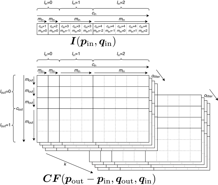
Figure 1: Example structure of the elements used in Eq. (8) when using two scalar ($l_{\mathrm{in}}=0$), one vector ($l_{\mathrm{in}}=1$), and one $l_{\mathrm{in}}=2$ input channels and three scalar ($l_{\mathrm{out}}=0$) and one vector ($l_{\mathrm{out}}=1$) output channels. The input features $\bm{I}(\bm{p}_{\mathrm{in}},\bm{q}_{\mathrm{in}})$ at point $(\bm{p}_{\mathrm{in}},\bm{q}_{\mathrm{in}})$ are a multi-channel spherical tensor consisting of multiple concatenated spherical tensors, the channels, indexed by $c_{\mathrm{in}}$, where the components of each channel are indexed by $m_{\mathrm{in}}$. A spherical tensor of order $l$ has $2l+1$ components (see Appendix A.2.1), so $\bm{I}(\bm{p}_{\mathrm{in}},\bm{q}_{\mathrm{in}})$ in this example has $\sum_{c_{\mathrm{in}}}2l(c_{\mathrm{in}})+1=2\cdot 1+1\cdot 3+1\cdot 5=10$ entries. The notation $\bm{C}\bm{F}(\bm{p}_{\mathrm{out}}-\bm{p}_{\mathrm{in}},\bm{q}_{\mathrm{out}},\bm{q}_{\mathrm{in}})$ is shorthand for the set $\left\{\sum_{m_{\mathrm{filter}}\in\{-l_{\mathrm{filter}},\dots,l_{\mathrm{filter}}\}}C_{(l_{\mathrm{filter}},m_{\mathrm{filter}})(\cdot,\cdot)}^{(\cdot,\cdot)}F_{m_{\mathrm{filter}}}^{(c_{\mathrm{filter}},k)}(\bm{p}_{\mathrm{out}}-\bm{p}_{\mathrm{in}},\bm{q}_{\mathrm{out}},\bm{q}_{\mathrm{in}})\right\}_{c_{\mathrm{filter}},k}$ over the indices $c_{\mathrm{filter}},k$, which is the filter $\bm{F}$ at position $(\bm{p}_{\mathrm{out}}-\bm{p}_{\mathrm{in}},\bm{q}_{\mathrm{out}},\bm{q}_{\mathrm{in}})$ combined with the CG coefficients $\bm{C}$. Each of the elements in this set is a matrix with the same number of columns as $\bm{I}(\bm{p}_{\mathrm{in}},\bm{q}_{\mathrm{in}})$ and the same number of rows as the resulting output spherical tensor $\bm{\mathcal{L}}[\bm{I}](\bm{p}_{\mathrm{out}},\bm{q}_{\mathrm{out}})$. Thus, $\bm{C}$ is applied linearly to the filter $\bm{F}$ and transforms it into a set of linear mappings from the input to the output multi-channel spherical tensors, where there is a linear mapping for each angular filter channel $c_{\mathrm{filter}}$ and radial basis index $k$. The linear mapping for each pair $c_{\mathrm{filter}},k$ contributes to the output by filtering the input with specific angular resolutions and radii.

Figure 2: Structure of the angular filter basis combined with $\bm{C}$. For a given radial basis index $k$, the filter $\bm{F}$ at position $(\bm{p}_{\mathrm{out}}-\bm{p}_{\mathrm{in}},\bm{q}_{\mathrm{out}},\bm{q}_{\mathrm{in}})$ combined with $\bm{C}$ (see Figure 1) can be decomposed into groups of angular filter channels $c_{\mathrm{filter}}$ of same order $l_{\mathrm{filter}}$, where $\oplus$ denotes the direct sum (concatenation). Note that the number of filter channels, i.e. possible values of $c_{\mathrm{filter}}$, for each order $l_{\mathrm{filter}}$ depends on the used angular basis. Thus, the shown stacked filter channels are meant to show that there might be multiple channels and should not be interpreted as the exact number of channels. If the angular basis filters are the spherical harmonics, then there is only one $c_{\mathrm{filter}}$ for each $l_{\mathrm{filter}}$. For each $l_{\mathrm{filter}}$, only specific elements can be non-zero (highlighted in grey), which follows from the properties of the CG coefficients. For $l_{\mathrm{filter}}=0$, the sections for $l_{\mathrm{out}}=0,l_{\mathrm{in}}=0$ represent the scalar-scalar product and the section for $l_{\mathrm{out}}=1,l_{\mathrm{in}}=1$ represents the vector-scalar product (each output component is based on the same input component) of input and filter. In $l_{\mathrm{filter}}=1$, the $l_{\mathrm{out}}=0,l_{\mathrm{in}}=1$ sections represent the dot product (the output is based on all components of the input), the $l_{\mathrm{out}}=1,l_{\mathrm{in}}=0$ sections represent the scalar-vector product (the input influences all output components), and the $l_{\mathrm{out}}=1,l_{\mathrm{in}}=1$ section represents the cross product (each input component influences all other output components but not the one at the same index). Figure 4 explains how the exact values in the red squares are obtained from the values $(\bm{p}_{\mathrm{out}}-\bm{p}_{\mathrm{in}},\bm{q}_{\mathrm{out}},\bm{q}_{\mathrm{in}})$ if the used angular basis are the spherical harmonics applied to one 3D space, e.g. $p$-space offsets as in Eq. (18), $q$-space offsets as in Eq. (19), or the space of differences between $p$- and $q$-space offsets in Eq. (20).

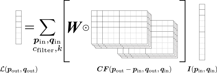
Figure 3: Interpretation of Eq. (8). At point $\bm{p}_{\mathrm{out}},\bm{q}_{\mathrm{out}}$ and for each possible $\bm{p}_{\mathrm{in}},\bm{q}_{\mathrm{in}}$, first $\bm{C}\bm{F}(\bm{p}_{\mathrm{out}}-\bm{p}_{\mathrm{in}},\bm{q}_{\mathrm{out}},\bm{q}_{\mathrm{in}})$ is built (see Figure 1). Then it is multiplied element-wise, denoted by $\odot$, with the trainable weights array $\bm{W}$. The result is matrix-multiplied (for each $c_{\mathrm{filter}},k$ independently) with $\bm{I}(\bm{p}_{\mathrm{in}},\bm{q}_{\mathrm{in}})$. Finally, we sum over all $\bm{p}_{\mathrm{in}},\bm{q}_{\mathrm{in}},c_{\mathrm{filter}},k$.

In order to define the proposed layer, for which Eq. (7) holds, Eq. (2) is generalized by adding dependence on $q$-space coordinates and replacing the angular filter order $l_{\mathrm{filter}}$ by the more general angular filter channel $c_{\mathrm{filter}}$:

$$\begin{split}\mathcal{L}_{m_{\mathrm{out}}}^{(c_{\mathrm{out}})}[\bm{I}](\bm{p}_{\mathrm{out}},\bm{q}_{\mathrm{out}})\coloneqq&\sum_{c_{\mathrm{in}},c_{\mathrm{filter}},k}W_{c_{\mathrm{in}},c_{\mathrm{out}},k}^{(c_{\mathrm{filter}})}\sum_{\begin{subarray}{c}m_{\mathrm{filter}}\in\{-l_{\mathrm{filter}},\dots,l_{\mathrm{filter}}\},\\ m_{\mathrm{in}}\in\{-l_{\mathrm{in}},\dots,l_{\mathrm{in}}\}\end{subarray}}C_{(l_{\mathrm{filter}},m_{\mathrm{filter}})(l_{\mathrm{in}},m_{\mathrm{in}})}^{(l_{\mathrm{out}},m_{\mathrm{out}})}\\ &\qquad\times\sum_{\begin{subarray}{c}\bm{p}_{\mathrm{in}}\in\mathbb{R}^{3},\\ \bm{q}_{\mathrm{in}}\in\mathbb{R}^{3}\end{subarray}}F_{m_{\mathrm{filter}}}^{(c_{\mathrm{filter}},k)}(\bm{p}_{\mathrm{out}}-\bm{p}_{\mathrm{in}},\bm{q}_{\mathrm{out}},\bm{q}_{\mathrm{in}})I_{m_{\mathrm{in}}}^{(c_{\mathrm{in}})}(\bm{p}_{\mathrm{in}},\bm{q}_{\mathrm{in}}),\end{split}$$ (8)

where $\bm{q}_{\mathrm{out}}$ and $\bm{q}_{\mathrm{in}}$ are $q$-space coordinates in the output and input feature map, respectively, $c_{\mathrm{filter}}$ is the angular filter channel index used to index the angular filter basis, $l_{\mathrm{filter}}$ is shorthand for $l(c_{\mathrm{filter}})$, i.e. the filter order of the angular filter channel given by $c_{\mathrm{filter}}$, $\bm{F}^{(c_{\mathrm{filter}},k)}$ are the basis filters, and the other variables and symbols are as in Eq. (2). We introduced the angular filter channel $c_{\mathrm{filter}}$ in order to allow generalization of the basis filters. While the filter basis defined in Eq. (4) contains only a single basis filter for given $k$ and $l_{\mathrm{filter}}$, we allow it to contain multiple of them so that there may be multiple angular filter channels $c_{\mathrm{filter}}$ for a given $l_{\mathrm{filter}}$, which is important for supporting filters built using the tensor product as we propose it. Like in Eq. (2), the decision which $l_{\mathrm{filter}}$ values to use for each path of information from a $c_{\mathrm{in}}$ to a $c_{\mathrm{out}}$ is a hyperparameter that can be freely chosen respecting Eq. (1). The number of angular filter channels $c_{\mathrm{filter}}$ for each $l_{\mathrm{filter}}$ then depends on the chosen angular basis and its hyperparameters. Note that following Thomas et al. (2018) the basis filters only depend on position differences as this is sufficient for translational equivariance in $p$-space, but we allow them to treat $\bm{q}_{\mathrm{out}}$ and $\bm{q}_{\mathrm{in}}$ independently as no translational equivariance is required in $q$-space. Figure 1 shows the intuitive structure of important elements of Eq. (8) for the example hyperparameters $\bm{\tau}_{\mathrm{in}}=(2,1,1),\bm{\tau}_{\mathrm{out}}=(3,1,0),c_{\mathrm{filter}}\in\{1,2,3,4\},k\in\{1,2\}$. Figure 2 shows some details of the angular basis combined with $\bm{C}$. Figure 3 gives an interpretation of Eq. (8) using the elements shown in Figure 1. Eq. (8) uses the definition of the tensor product from Eq. (33) and, analogously to Eq. (3), the layer could instead be defined using the tensor product explicitly:

$$\begin{split}&\mathcal{L}_{m_{\mathrm{out}}}^{(c_{\mathrm{out}})}[\bm{I}](\bm{p}_{\mathrm{out}},\bm{q}_{\mathrm{out}})\\ &\qquad\coloneqq\sum_{c_{\mathrm{in}},c_{\mathrm{filter}},k}W_{c_{\mathrm{in}},c_{\mathrm{out}},k}^{(c_{\mathrm{filter}})}\sum_{\begin{subarray}{c}\bm{p}_{\mathrm{in}}\in\mathbb{R}^{3},\\ \bm{q}_{\mathrm{in}}\in\mathbb{R}^{3}\end{subarray}}\Big{(}\bm{F}^{(c_{\mathrm{filter}},k)}(\bm{p}_{\mathrm{out}}-\bm{p}_{\mathrm{in}},\bm{q}_{\mathrm{out}},\bm{q}_{\mathrm{in}})\otimes\bm{I}^{(c_{\mathrm{in}})}(\bm{p}_{\mathrm{in}},\bm{q}_{\mathrm{in}})\Big{)}_{m_{\mathrm{out}}}^{l_{\mathrm{out}}}.\end{split}$$ (9)

We require that all basis filters $\bm{F}^{(c_{\mathrm{filter}},k)}$ are equivariant under joint rotations:

$$\bm{F}^{(c_{\mathrm{filter}},k)}(\bm{\mathcal{R}}_{g}\Delta\bm{p},\bm{\mathcal{R}}_{g}\bm{q}_{\mathrm{out}},\bm{\mathcal{R}}_{g}\bm{q}_{\mathrm{in}})=\bm{D}^{(l_{\mathrm{filter}})}_{g}\bm{F}^{(c_{\mathrm{filter}},k)}(\Delta\bm{p},\bm{q}_{\mathrm{out}},\bm{q}_{\mathrm{in}}),$$ (10)

which is an extension of the $\mathrm{SO}(3)$-equivariance required for Eq. (4), and implies the required equivariance of the layer, as proved in Appendix D.1.

3.2.2 General Filter Basis

Each basis filter $\bm{F}^{(c_{\mathrm{filter}},k)}\colon\left(\mathbb{R}^{3}\right)^{3}\to\mathcal{S}^{l_{\mathrm{filter}}}$ maps the tuple $(\Delta\bm{p},\bm{q}_{\mathrm{out}},\bm{q}_{\mathrm{in}})\in\left(\mathbb{R}^{3}\right)^{3}$ (the position difference $\Delta\bm{p}=\bm{p}_{\mathrm{out}}-\bm{p}_{\mathrm{in}}$ and the two $q$-space coordinates $\bm{q}_{\mathrm{out}}$ and $\bm{q}_{\mathrm{in}}$) to a spherical tensor of order $l_{\mathrm{filter}}$. This filter tensor will later be applied (using the tensor product) to the input feature map. As in Eq. (4), the basis filter consists of a radial basis and an angular basis, which we generalize to functions $R^{(k)}\colon\left(\mathbb{R}^{3}\right)^{3}\to\mathbb{R}$ and $\bm{A}^{(c_{\mathrm{filter}})}\colon\left(\mathbb{R}^{3}\right)^{3}\to\mathcal{S}^{l_{\mathrm{filter}}}$, respectively. Thus, $\bm{F}^{(c_{\mathrm{filter}},k)}$ is defined as

$$\bm{F}^{(c_{\mathrm{filter}},k)}(\Delta\bm{p},\bm{q}_{\mathrm{out}},\bm{q}_{\mathrm{in}})\coloneqq R^{(k)}(\Delta\bm{p},\bm{q}_{\mathrm{out}},\bm{q}_{\mathrm{in}})\bm{A}^{(c_{\mathrm{filter}})}(\Delta\bm{p},\bm{q}_{\mathrm{out}},\bm{q}_{\mathrm{in}}).$$ (11)

We require $R$ to be invariant under rotations:

$$R^{(k)}(\bm{\mathcal{R}}_{g}\Delta\bm{p},\bm{\mathcal{R}}_{g}\bm{q}_{\mathrm{out}},\bm{\mathcal{R}}_{g}\bm{q}_{\mathrm{in}})=R^{(k)}(\Delta\bm{p},\bm{q}_{\mathrm{out}},\bm{q}_{\mathrm{in}})\qquad\forall g\in\mathrm{SO}(3),$$ (12)

and $\bm{A}$ to be equivariant under rotations:

$$\bm{A}^{(c_{\mathrm{filter}})}(\bm{\mathcal{R}}_{g}\Delta\bm{p},\bm{\mathcal{R}}_{g}\bm{q}_{\mathrm{out}},\bm{\mathcal{R}}_{g}\bm{q}_{\mathrm{in}})=\bm{D}^{(l_{\mathrm{filter}})}_{g}\bm{A}^{(c_{\mathrm{filter}})}(\Delta\bm{p},\bm{q}_{\mathrm{out}},\bm{q}_{\mathrm{in}})\qquad\forall g\in\mathrm{SO}(3),$$ (13)

as this is sufficient for $\bm{F}$ (11) to satisfy Eq. (10) as is proven in Appendix D.2. Various options for $R$ and $\bm{A}$ are described in Section 3.2.3 and Section 3.2.4, respectively, and in Section 3.2.5 we propose basis filters built using these options.

3.2.3 Radial Filter Basis

We use the following simple forms for the radial basis:

• a radial basis using only $\Delta\bm{p}$, as in Eq. (4):

  $$R_{p\text{-diff}}^{(k)}(\Delta\bm{p},\bm{q}_{\mathrm{out}},\bm{q}_{\mathrm{in}})\coloneqq\varphi^{(k)}\left(\left\lVert\Delta\bm{p}\right\rVert_{2}\right),$$ (14)

• a radial basis using only $q$-space coordinates of the input feature map, a proposed adaption of Eq. (14):

  $$R_{q\text{-in}}^{(k)}(\Delta\bm{p},\bm{q}_{\mathrm{out}},\bm{q}_{\mathrm{in}})\coloneqq\varphi^{(k)}\left(\left\lVert\bm{q}_{\mathrm{in}}\right\rVert_{2}\right),$$ (15)

• and a radial basis using only $q$-space coordinates of the output feature map, a proposed adaption of Eq. (14):

  $$R_{q\text{-out}}^{(k)}(\Delta\bm{p},\bm{q}_{\mathrm{out}},\bm{q}_{\mathrm{in}})\coloneqq\varphi^{(k)}\left(\left\lVert\bm{q}_{\mathrm{out}}\right\rVert_{2}\right),$$ (16)

where $\varphi^{(k)}\colon\mathbb{R}_{\geq 0}\to\mathbb{R}$ is a set of radial basis functions, e.g. Gaussian radial basis functions (Weiler et al., 2018b), cosine radial basis functions (Geiger et al., 2020), or a fully connected network applied to a set of basis functions (Thomas et al., 2018; Geiger et al., 2020). For details on the radial basis functions, see Appendix B.1.

We propose to combine multiple radial bases multiplicatively:

$$R_{\text{prod}}^{(k)}(\Delta\bm{p},\bm{q}_{\mathrm{out}},\bm{q}_{\mathrm{in}})=R_{\text{prod}}^{(k_{1},k_{2})}(\Delta\bm{p},\bm{q}_{\mathrm{out}},\bm{q}_{\mathrm{in}})\coloneqq R^{(k_{1})}_{1}(\Delta\bm{p},\bm{q}_{\mathrm{out}},\bm{q}_{\mathrm{in}})R^{(k_{2})}_{2}(\Delta\bm{p},\bm{q}_{\mathrm{out}},\bm{q}_{\mathrm{in}}),$$ (17)

where $R^{(k_{1})}_{1}$ and $R^{(k_{2})}_{2}$ are the two radial bases being combined and each value assumed by $k$ represents one of the possible combinations of the radial basis indices $k_{1}$ and $k_{2}$ of the two combined radial bases. This means that the radial basis size $K$ is the product of the sizes $K_{1},K_{2}$ of the two combined radial bases: $K=K_{1}K_{2}$.

3.2.4 Angular Filter Basis

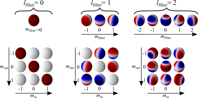
Figure 4: Visualization of the spherical harmonics and their combination with the CG coefficients. As the domain of the spherical harmonics is the sphere, they can be represented using a colored sphere for each $l_{\mathrm{filter}},m_{\mathrm{filter}}$, where the point on the sphere represents the direction of the vector given to the spherical harmonic, i.e. the direction of $\bm{p}_{\mathrm{out}}-\bm{p}_{\mathrm{in}}$ in $\bm{A}_{p\text{-diff}}$, of $\bm{q}_{\mathrm{out}}-\bm{q}_{\mathrm{in}}$ in $\bm{A}_{q\text{-diff}}$, and of $(\bm{p}_{\mathrm{out}}-\bm{q}_{\mathrm{out}})-(\bm{p}_{\mathrm{in}}-\bm{q}_{\mathrm{in}})$ in $\bm{A}_{pq\text{-diff}}$, respectively. In the upper part of the figure, the spherical harmonics $Y_{m_{\mathrm{filter}}}^{l_{\mathrm{filter}}}$ of orders $l_{\mathrm{filter}}=0,1,2$ are shown. When used as angular filters for vector input and output ($l_{\mathrm{in}}=l_{\mathrm{out}}=1$), they can be combined with the CG coefficients $\bm{C}_{0,1}^{1}$, $\bm{C}_{1,1}^{1}$, and $\bm{C}_{2,1}^{1}$, respectively. The results of this combination are shown in the lower part of the figure. By applying these angular basis functions to the aforementioned direction vector, we obtain the three $3\times 3$ matrices in the ($l_{\mathrm{in}}=l_{\mathrm{out}}=1$) section of the filter, shown as red squares in Figure 2.

We use the following angular bases, all based on the (real) spherical harmonics $\bm{Y}$ (see Appendix A.2.1):

• an angular basis using only $\Delta\bm{p}$, as in Eq. (4):

  $$\bm{A}^{(c_{\mathrm{filter}})}_{p\text{-diff}}(\Delta\bm{p},\bm{q}_{\mathrm{out}},\bm{q}_{\mathrm{in}})\coloneqq\bm{Y}^{(l_{\mathrm{filter}})}\left(\frac{\Delta\bm{p}}{\left\lVert\Delta\bm{p}\right\rVert_{2}}\right)=\bm{Y}^{(l_{\mathrm{filter}})}_{m_{\mathrm{filter}}}\left(\frac{\bm{p}_{\mathrm{out}}-\bm{p}_{\mathrm{in}}}{\left\lVert\bm{p}_{\mathrm{out}}-\bm{p}_{\mathrm{in}}\right\rVert_{2}}\right),$$ (18)

• an angular basis using only the $q$-difference, i.e. the offset between input and output $q$-space coordinates, a proposed adaption of Eq. (18):

  $$\bm{A}^{(c_{\mathrm{filter}})}_{q\text{-diff}}(\Delta\bm{p},\bm{q}_{\mathrm{out}},\bm{q}_{\mathrm{in}})\coloneqq\bm{Y}^{(l_{\mathrm{filter}})}\left(\frac{\bm{q}_{\mathrm{out}}-\bm{q}_{\mathrm{in}}}{\left\lVert\bm{q}_{\mathrm{out}}-\bm{q}_{\mathrm{in}}\right\rVert_{2}}\right),$$ (19)

• and an angular basis using the $pq$-difference, i.e. the difference between the input/output offsets of $p$- and $q$-space coordinates, which is the same as the input/output offsets of the differences between $p$- and $q$-space coordinates, a proposed adaption of Eq. (18):

  $$\begin{split}\bm{A}^{(c_{\mathrm{filter}})}_{pq\text{-diff}}(\Delta\bm{p},\bm{q}_{\mathrm{out}},\bm{q}_{\mathrm{in}})\coloneqq{}&\bm{Y}^{(l_{\mathrm{filter}})}\left(\frac{\Delta\bm{p}-(\bm{q}_{\mathrm{out}}-\bm{q}_{\mathrm{in}})}{\left\lVert\Delta\bm{p}-(\bm{q}_{\mathrm{out}}-\bm{q}_{\mathrm{in}})\right\rVert_{2}}\right)\\ ={}&\bm{Y}^{(l_{\mathrm{filter}})}\left(\frac{(\bm{p}_{\mathrm{out}}-\bm{q}_{\mathrm{out}})-(\bm{p}_{\mathrm{in}}-\bm{q}_{\mathrm{in}})}{\left\lVert(\bm{p}_{\mathrm{out}}-\bm{q}_{\mathrm{out}})-(\bm{p}_{\mathrm{in}}-\bm{q}_{\mathrm{in}})\right\rVert_{2}}\right),\end{split}$$ (20)

where $l_{\mathrm{filter}}$ is shorthand for $l(c_{\mathrm{filter}})$, i.e. the filter order of the angular filter channel given by $c_{\mathrm{filter}}$. The intuition of $\bm{A}_{pq\text{-diff}}$ is that the spherical harmonics expect a 3D unit vector as input and we want it to depend on $p$- and $q$-space coordinates, so both coordinates need to be combined to another 3D unit vector in an equivariant way. We choose the difference operation as it is a very simple linear operation. Figure 4 visualizes the spherical harmonics and their combination with the CG coefficients. As the introduced angular bases $\bm{A}_{p\text{-diff}}$, $\bm{A}_{q\text{-diff}}$, and $\bm{A}_{pq\text{-diff}}$ are all based on the spherical harmonics, this figure also provides some intuition about these bases.

Table 1: Visualization of the angular basis $\bm{A}_{\text{TP}}$, Eq. (21), for the filter order $l_{\mathrm{filter}}=0,1$, and the orders $l_{1}=0,1$ and $l_{2}=0,1$ of the angular bases $\bm{A_{1}}$ and $\bm{A_{2}}$ being combined. As the bases $\bm{A_{1}}$ and $\bm{A_{2}}$ are not defined specifically, i.e. they may be any function with specific properties, $\bm{A}_{\text{TP}}$ cannot be visualized in general. Therefore, we visualize a specific variant of $\bm{A}_{\text{TP}}$ where $\bm{A_{1}}$ and $\bm{A_{2}}$ are the spherical harmonics applied to $p$- and $q$-space coordinate offsets, respectively, i.e. $l_{1}=l_{p}$, $l_{2}=l_{q}$, $\left(\bm{A}_{1}\right)^{(l_{1})}=\bm{Y}^{(l_{p})}\left(\frac{\Delta\bm{p}}{\left\lVert\Delta\bm{p}\right\rVert_{2}}\right)$, $\left(\bm{A}_{2}\right)^{(l_{2})}=\bm{Y}^{(l_{q})}\left(\frac{\bm{q}_{\mathrm{out}}-\bm{q}_{\mathrm{in}}}{\left\lVert\bm{q}_{\mathrm{out}}-\bm{q}_{\mathrm{in}}\right\rVert_{2}}\right)$. With this definition, $\bm{A}_{\text{TP}}$ corresponds to the angular part of $\bm{F}_{\text{TP}}$ as defined in Eq. (26). The domain of $\bm{A_{1}}$, $\bm{A_{2}}$, and $\bm{A}_{\text{TP}}$ consists of 6D directions, i.e. the directions of the two 3D vectors $\Delta\bm{p}$ and $(\bm{q}_{\mathrm{out}}-\bm{q}_{\mathrm{in}})$. We project it to 3D for visualization purposes by plotting the azimuthal angle from the first 3D space ($\Delta\bm{p}$) and the polar angle from the second 3D space $(\bm{q}_{\mathrm{out}}-\bm{q}_{\mathrm{in}})$ and fixing the other angles to constant values. Thus, even if plotted spheres are equal, the non-projected values may not be. In the rows with $l_{\mathrm{filter}}=1$ and $l_{1}=0$ or $l_{2}=0$ it can be seen that the resulting $\bm{A}_{\text{TP}}$ only depends on $\bm{A_{2}}$ (i.e. the content of the blue rectangles is identical) or $\bm{A_{1}}$ (i.e. the content of the orange rectangles is identical), respectively. This is because $\left(\bm{A}_{1}\right)^{(0)}$ and $\left(\bm{A}_{2}\right)^{(0)}$ are scalars and thus independent of directions.

$l_{\mathrm{filter}}$	$l_{1}$	$l_{2}$	$\left(\bm{A}_{1}\right)^{(l_{1})}$	$\left(\bm{A}_{2}\right)^{(l_{2})}$	$\left(\bm{A}\right)_{\text{TP}}^{(l_{\mathrm{filter}},l_{1},l_{2})}$
	$l_{p}$	$l_{q}$	$\bm{Y}^{(l_{p})}\left(\frac{\Delta\bm{p}}{\left\lVert\Delta\bm{p}\right\rVert_{2}}\right)$	$\bm{Y}^{(l_{q})}\left(\frac{\bm{q}_{\mathrm{out}}-\bm{q}_{\mathrm{in}}}{\left\lVert\bm{q}_{\mathrm{out}}-\bm{q}_{\mathrm{in}}\right\rVert_{2}}\right)$	$\bm{F}_{\text{TP}}^{(l_{\mathrm{filter}},l_{p},l_{q})}$
			$m_{1}=-1\qquad 0\qquad+1$	$m_{2}=-1\qquad 0\qquad+1$	$m_{\mathrm{filter}}=-1\qquad 0\qquad+1\qquad$
0	0	0
0	1	1
1	0	1
1	1	0
1	1	1

Instead of combining the $p$- and $q$-space coordinates before applying the spherical harmonics, we also propose to combine two angular bases $\left(\bm{A}_{1}\right)^{(c_{1})}$ and $\left(\bm{A}_{2}\right)^{(c_{2})}$, which may depend on $p$- and $q$-space coordinates, respectively, using the tensor product (as defined in Eq. (33)):

$$\begin{split}\left(A_{\text{TP}}\right)^{(c_{\mathrm{filter}})}_{m_{\mathrm{filter}}}(\Delta\bm{p},\bm{q}_{\mathrm{out}},\bm{q}_{\mathrm{in}})=&\left(A_{\text{TP}}\right)^{(l_{\mathrm{filter}},c_{1},c_{2})}_{m_{\mathrm{filter}}}(\Delta\bm{p},\bm{q}_{\mathrm{out}},\bm{q}_{\mathrm{in}})\\ \coloneqq&\sum_{\begin{subarray}{c}m_{1}\in\{-l_{1},\dots,l_{1}\},\\ m_{2}\in\{-l_{2},\dots,l_{2}\}\end{subarray}}C_{(l_{1},m_{1})(l_{2},m_{2})}^{(l_{\mathrm{filter}},m_{\mathrm{filter}})}\\ &\qquad\times\left(A_{1}\right)^{(c_{1})}_{m_{1}}(\Delta\bm{p},\bm{q}_{\mathrm{out}},\bm{q}_{\mathrm{in}})\left(A_{2}\right)^{(c_{2})}_{m_{2}}(\Delta\bm{p},\bm{q}_{\mathrm{out}},\bm{q}_{\mathrm{in}}),\end{split}$$ (21)

where each value assumed by $c_{\mathrm{filter}}$ represents one combination of filter order $l_{\mathrm{filter}}$ and angular basis channels $c_{1}$, $c_{2}$ of the angular bases $\bm{A}_{1},\bm{A}_{2}$ that are being combined, $l_{1},l_{2}$ denote the orders these channels, and $m_{\mathrm{filter}}$ is the index of the components of the spherical tensors produced by the filter for given $c_{\mathrm{filter}}$, with $-l_{\mathrm{filter}}\leq m_{\mathrm{filter}}\leq l_{\mathrm{filter}}$. When building filter channels of a given filter order $l_{\mathrm{filter}}$, the orders $l_{1},l_{2}$ can be freely chosen as long as they satisfy the following constraint, which follows from the properties of the Clebsch–Gordan coefficients as defined in Eq. (34):

$$|l_{1}-l_{2}|\leq l_{\mathrm{filter}}\leq(l_{1}+l_{2}).$$ (22)

Table 1 visualizes the angular basis $\bm{A}_{\text{TP}}$ and provides some intuition.

3.2.5 Proposed Filter Bases

Using the angular and radial parts discussed in Section 3.2.3 and Section 3.2.4, various variants of filter bases can be built. As proven in Appendix D.2, the equivariance of these filter bases follows from the invariance of their radial parts, proven in Appendix D.3, and the equivariance of their angular parts, proven in Appendix D.4. In this work, the following filter bases are proposed:

$p$-Space Filter

The following filter basis depends only on $p$-space coordinates and is built using the $p$-difference radial basis (14) and the $p$-difference angular basis (18):

$$\begin{split}F_{p\text{-space},m_{\mathrm{filter}}}^{(c_{\mathrm{filter}},k)}(\Delta\bm{p},\bm{q}_{\mathrm{out}},\bm{q}_{\mathrm{in}})={}&F_{p\text{-space},m_{\mathrm{filter}}}^{(l_{\mathrm{filter}},k)}(\Delta\bm{p},\bm{q}_{\mathrm{out}},\bm{q}_{\mathrm{in}})\\ \coloneqq{}&\varphi^{(k)}(\left\lVert\Delta\bm{p}\right\rVert_{2})Y_{m_{\mathrm{filter}}}^{(l_{\mathrm{filter}})}\left(\frac{\Delta\bm{p}}{\left\lVert\Delta\bm{p}\right\rVert_{2}}\right).\end{split}$$ (23)

$q$-Space Filter

The following filter basis depends only on $q$-space coordinates and is built using the multiplicative combination (17) of the $q$-in (15) and $q$-out (16) radial bases, and using the $q$-difference angular basis (19):

$$\begin{split}F_{q\text{-space},m_{\mathrm{filter}}}^{(c_{\mathrm{filter}},k)}(\Delta\bm{p},\bm{q}_{\mathrm{out}},\bm{q}_{\mathrm{in}})={}&F_{q\text{-space},m_{\mathrm{filter}}}^{(l_{\mathrm{filter}},k_{1},k_{2})}(\Delta\bm{p},\bm{q}_{\mathrm{out}},\bm{q}_{\mathrm{in}})\\ \coloneqq{}&\varphi^{(k_{1})}(\left\lVert\bm{q}_{\mathrm{out}}\right\rVert_{2})\varphi^{(k_{2})}(\left\lVert\bm{q}_{\mathrm{in}}\right\rVert_{2})Y_{m_{\mathrm{filter}}}^{(l_{\mathrm{filter}})}\left(\frac{\bm{q}_{\mathrm{out}}-\bm{q}_{\mathrm{in}}}{\left\lVert\bm{q}_{\mathrm{out}}-\bm{q}_{\mathrm{in}}\right\rVert_{2}}\right).\end{split}$$ (24)

$pq$-difference Filter

The following filter basis depends on $p$- and $q$-space coordinates and is built using the multiplicative combination (17) of the $p$-difference (14), $q$-in (15), and $q$-out (16) radial bases, and using the $pq$-difference angular basis (20):

$$\begin{split}F_{pq\text{-diff},m_{\mathrm{filter}}}^{(c_{\mathrm{filter}},k)}(\Delta\bm{p},\bm{q}_{\mathrm{out}},\bm{q}_{\mathrm{in}})={}&F_{pq\text{-diff},m_{\mathrm{filter}}}^{(l_{\mathrm{filter}},k_{1},k_{2},k_{3})}(\Delta\bm{p},\bm{q}_{\mathrm{out}},\bm{q}_{\mathrm{in}})\\ \coloneqq{}&\varphi^{(k_{1})}(\left\lVert\Delta\bm{p}\right\rVert_{2})\varphi^{(k_{2})}(\left\lVert\bm{q}_{\mathrm{out}}\right\rVert_{2})\varphi^{(k_{3})}(\left\lVert\bm{q}_{\mathrm{in}}\right\rVert_{2})\\ &\qquad\times Y_{m_{\mathrm{filter}}}^{(l_{\mathrm{filter}})}\left(\frac{\Delta\bm{p}-(\bm{q}_{\mathrm{out}}-\bm{q}_{\mathrm{in}})}{\left\lVert\Delta\bm{p}-(\bm{q}_{\mathrm{out}}-\bm{q}_{\mathrm{in}})\right\rVert_{2}}\right).\end{split}$$ (25)

Tensor Product of $p$- and $q$-Space Filters

The following filter basis depends on $p$- and $q$-space coordinates and is built using the multiplicative combination (17) of the $p$-difference (14), $q$-in (15), and $q$-out (16) radial bases, and using the tensor product combination (21) of the $p$-difference (18) and $q$-difference (19) angular bases:

$$\begin{split}F_{\text{TP},m_{\mathrm{filter}}}^{(c_{\mathrm{filter}},k)}(\Delta\bm{p},\bm{q}_{\mathrm{out}},\bm{q}_{\mathrm{in}})={}&F_{\text{TP},m_{\mathrm{filter}}}^{(l_{\mathrm{filter}},l_{p},l_{q},k_{1},k_{2},k_{3})}(\Delta\bm{p},\bm{q}_{\mathrm{out}},\bm{q}_{\mathrm{in}})\\ \coloneqq{}&\varphi^{(k_{1})}(\left\lVert\Delta\bm{p}\right\rVert_{2})\varphi^{(k_{2})}(\left\lVert\bm{q}_{\mathrm{out}}\right\rVert_{2})\varphi^{(k_{3})}(\left\lVert\bm{q}_{\mathrm{in}}\right\rVert_{2})\\ &\qquad\times\sum_{\begin{subarray}{c}m_{p}\in\{-l_{p},\dots,l_{p}\},\\ m_{q}\in\{-l_{q},\dots,l_{q}\}\end{subarray}}C_{(l_{p},m_{p})(l_{q},m_{q})}^{(l_{\mathrm{filter}},m_{\mathrm{filter}})}\\ &\qquad\times Y_{m_{p}}^{(l_{p})}\left(\frac{\Delta\bm{p}}{\left\lVert\Delta\bm{p}\right\rVert_{2}}\right)Y_{m_{q}}^{(l_{q})}\left(\frac{\bm{q}_{\mathrm{out}}-\bm{q}_{\mathrm{in}}}{\left\lVert\bm{q}_{\mathrm{out}}-\bm{q}_{\mathrm{in}}\right\rVert_{2}}\right),\end{split}$$ (26)

where $l_{p},l_{q}$ (inserted for $l_{1},l_{2}$ in Eq. (21)) are the orders of the $p$- and $q$-space filters, i.e. the orders of the spherical harmonics applied to $p$- and $q$-space, respectively, and given the filter order $l_{\mathrm{filter}}$, may be selected freely respecting Eq. (22) (with $l_{p},l_{q}$ inserted for $l_{1},l_{2}$).

Thus, given an input of type $\bm{\tau}_{\mathrm{in}}$ (the numbers of input channels of each order $l_{\mathrm{in}}$), the hyperparameter selection process is as follows: 1. select output type $\bm{\tau}_{\mathrm{out}}$ (the numbers of output channels of each order $l_{\mathrm{out}}$), 2. for each pair $(c_{\mathrm{in}},c_{\mathrm{out}})$, choose what $l_{\mathrm{filter}}$ values to use (respecting Eq. (1)), 3. in the case of the TP filter, choose what $(l_{p},l_{q})$ tuples to use for each $l_{\mathrm{filter}}$ (respecting Eq. (22) with $l_{p},l_{q}$ inserted for $l_{1},l_{2}$).

Each tuple $(l_{\mathrm{filter}},l_{p},l_{q})$ represents a specific operation (as per Eq. 33) used to combine the $p$- and $q$-space filters, e.g. the cross product in the case of $(1,1,1)$ or the dot product for $(0,1,1)$. As for a given $l_{\mathrm{filter}}$ there may be multiple possible options for $l_{p}$ and $l_{q}$, the angular basis may contain several basis filters for each $l_{\mathrm{filter}}$.

There may be many different strategies to choose the set of $(l_{\mathrm{filter}},l_{p},l_{q})$. We focus on analyzing the effect of the angular basis size and thus choose two strategies, one with a small set of $(l_{\mathrm{filter}},l_{p},l_{q})$, which thus has very few angular basis filters, and the other with a larger set and thus more basis filters.

In the first strategy we focus on operations on vectors, as vectors are the lowest-order tensors that can represent directions and as such enable us to consider directions with minimum possible effort. Thus, we use the cross product and scalar products, represented by tuples $(l_{\mathrm{filter}},l_{p},l_{q})$ with values $(1,1,1)$, $(1,0,1)$, and $(1,1,0)$. To also support basis filters of order $l_{\mathrm{filter}}=0$ and $l_{\mathrm{filter}}=2$, respectively, which are the neighboring filter orders of $l_{\mathrm{filter}}=1$, the tuples $(0,0,0)$ and $(2,2,2)$ are included. Note that this hyperparameter choice is free and we might have also chosen to not include them or to use different $l_{p},l_{q}$. The filter basis using $F_{\text{TP}}$ (26) with the described strategy will be called $F_{\text{TP-vec}}$.

In the other strategy used to create a larger angular basis, certain rules are defined regarding which $(l_{\mathrm{filter}},l_{p},l_{q})$ to select. Besides constraint (22), we choose $(l_{\mathrm{filter}},l_{p},l_{q})$ such that $l_{p}$ and $l_{q}$ do not deviate from the given $l_{\mathrm{filter}}$ more than by an integer hyperparameter $d$, meaning that $|l_{\mathrm{filter}}-l_{p}|\leq d$ and $|l_{\mathrm{filter}}-l_{q}|\leq d$. While this rule is arbitrary to create filter bases much larger than $F_{\text{TP-vec}}$ while still restricting the number of basis filters to a finite number, which is not restricted by constraint (22), the intuition behind this rule is to create filters from $p$- and $q$-space filters of orders $l_{p},l_{q}$ close to the resulting filter order $l_{\mathrm{filter}}$. We call the filter basis based on $F_{\text{TP}}$ (26) with this strategy applied $F_{\text{TP}\pm d}$, e.g. $F_{\text{TP}\pm 1}$ for $d=1$.

3.2.6 Comparison and Combinations of the Proposed Filter Bases

The filter bases $F_{p\text{-space}}$ (23) and $F_{q\text{-space}}$ (24) each only depend on coordinates of one space, $p$- and $q$-space, respectively, thus they are invariant under rotations and translations in the other space. While some invariances might be wanted for the whole network, it may lead to drawbacks if early layers are invariant. Later layers extract higher-level features and if early layers are invariant then some information required for the higher-level features might be lost.

The $F_{pq\text{-diff}}$ basis (25) depends on coordinates from both spaces. But it discards parts of the structural information of the input (not the image values), as its angular part only depends on the difference of coordinate offsets of the two spaces, which means that the structural information from coordinates in both 3D spaces is represented by only a single 3D vector.

To solve this problem, the $F_{pq\text{-diff}}$ basis may be combined with the $F_{p\text{-space}}$ or the $F_{q\text{-space}}$ basis by filtering the feature maps with both filters independently and then combining the results by summing. (Summing is like using more filter channels.) These filter bases will be called $F_{pq\text{-diff}+p}$ and $F_{pq\text{-diff}+q}$. As $F_{pq\text{-diff}}$ and $F_{p\text{-space}}$ depend on different 3D vectors which together contain all relevant structural information, $F_{pq\text{-diff}+p}$ does not discard parts of the structural information of the input. The same is true for the combination of $F_{pq\text{-diff}}$ and $F_{q\text{-space}}$ to $F_{pq\text{-diff}+q}$.

The filter basis $F_{\text{TP}}$ (26), and its variants $F_{\text{TP-vec}}$ and $F_{\text{TP}\pm d}$, use structural information from both $p$- and $q$-space by combining angular basis filters of these two spaces using multiple operations, defined by the tensor product, and thus may access more aspects of the structural dependencies between both spaces than filters using $F_{pq\text{-diff}}$, which only uses as single operation, the difference. As the angular part of $F_{\text{TP}}$ (26), in contrast to all other bases like $F_{pq\text{-diff}+p}$, may contain several basis filters for each $l_{\mathrm{filter}}$, it has the largest number of parameters (as the $\bm{W}$ is larger if the basis contains more basis filters), most computational effort, and highest memory requirements for the same number and orders of input and output channels.

3.2.7 Implementation of the Layer

Details on the implementation of the layer are given in Appendix B. Our code is available at https://github.com/philip-mueller/equivariant-deep-dmri#. In order to use the layer with dMRI scans, i.e. with finite Cartesian $p$-space and finite sampling schemes in $q$-space, Eq. (8) needs to be discretized as explained in Appendix B.3. We follow Weiler et al. (2018b), where the precomputation of parts of the filter is proposed for a computationally efficient and hardware-optimized implementation on voxel grids, and implement Eq. (8) using 3D convolutional layers as explained in Appendix B.4.

4 Experimental Setup

The effectivity of the proposed layer was studied by doing segmentation (i.e. voxel-wise classification) of multiple sclerosis (MS) lesions using a dataset (Lipp et al., 2017; 2020) containing dMRI brain scans with ground-truth annotations of MS lesions.

4.1 Dataset and Preprocessing

The dMRI scans are sampled at 46 $q$-space points: six times at $\bm{q}=\bm{0}$, and at 40 uniformly distributed diffusion directions ($b=1200\mathrm{s/mm}^{2}$, SE-EPI, voxel size $1.8\mathrm{mm}\times 1.8\mathrm{mm}\times 2.4\mathrm{mm}$, matrix $128\times 128$, $57$ slices, TE=94.5ms, TR=16s, motion/distortion-corrected with elastix (Klein et al., 2010) with upsampling to $256\times 256\times 172$). For well-behaved neural network training, so-called feature scaling was performed by dividing each channel by the corresponding channel mean taken over all scans. To prevent overfitting on intensity values, each scan was additionally divided by its mean intensity. The ground truth of each sample describes for each voxel whether it contains any MS lesion or not, so it has the same resolution as the scan but does not contain different $q$-space points.

Due to the long training times, no cross-validation was performed. Instead, the dataset (94 MS patients) was split only once into training and validation set at an 80/20 ratio.

As the directed $q$-vectors slightly differ between the scans (due to motion correction), the mean of each of these $q$-vectors over all training samples was used as the input $q$-sampling scheme of the network (exact $q$-vectors could be considered, but would require precomputing more filters or recomputing larger parts of the filters in each iteration).

4.2 Network Architecture

A simple architecture is chosen that first combines all $\bm{q}=\bm{0}$ channels by computing their mean, then applies multiple of the proposed equivariant layers on $p$- and $q$-space (they will be referred to as $pq$-layers), followed by a global reduction operation (called $q$-reduction) that “collapses” $q$-space and only leaves $p$-space, and then applies multiple of the proposed equivariant layers on $p$-space (called $p$-layers).

$pq$-layers

In this work the following filter bases for the $pq$-layers are investigated (see Section 3.2.6 for details): $F_{pq\text{-diff}+p}$, $F_{pq\text{-diff}+q}$, $F_{\text{TP-vec}}$, and $F_{\text{TP}\pm 1}$.

$q$-reduction

There are several options how the $q$-space can be “collapsed” but in this work the comparison is focused on the following two configurations:

• late: In all $pq$-layers the same $q$-sampling scheme as in the input data is used. The $q$-space is then “collapsed” using a q-length weighted average layer, which applies radial basis functions on the lengths of the $q$-vectors in the sampling scheme and weights the results using learned weights.

• gradual: Each $pq$-layer uses a different output $q$-sampling scheme $\mathcal{Q}_{\mathrm{out}}$ that consists of less $q$-vectors than in the layer before. The final $q$-reduction is done using the same filtering as in the $pq$-layers but with $\mathcal{Q}_{\mathrm{out}}=\{(0,0,0)\}$.

$p$-layers

As in the $p$-layers no $q$-space is present anymore, only the $F_{p\text{-space}}$ (23) filter basis is used. Note that this is equivalent to the layer defined in Eq. (2).

Further Configuration

Various channel configurations used in this work are defined in Appendix E.1. Swish (Ramachandran et al., 2017) is used as acitvation function for scalar channels and the gated nonlinearity (Weiler et al., 2018b) is used for $l>0$ channels (see Appendix B.2). In $q$-space we use Gaussian radial basis functions (37) and in $p$-space we either use cosine radial basis functions (38) or Gaussian radial basis functions and either apply three fully connected (FC) layers, having 50 neurons each, to them (cosine+fc/Gaussian+fc) or use them alone (cosine/Gaussian). In the kernels, all possible orders $l_{\mathrm{filter}}$ (see Eq. (1)) of angular basis filters are used and the kernel size in $p$-space is set to $5$.

4.3 Training

Binary cross-entropy is used as loss and the sigmoid function is used as activation function in the final layer. Using the brain masks of each sample, all voxels outside of the brain are ignored when computing the loss and the quality metrics. To counteract class imbalance, positive and negative voxels were weighted in the loss according to the ratio between positive and negative voxels in the whole training set.

Due to the large feature maps, much GPU memory was required during training. To reduce the required memory to a minimum, only a batch size of one was used and each sample was cropped to the bounding box defined by its brain mask. Additionally, checkpointing was applied, where only some feature maps at defined checkpoints are stored in each forward pass and the other ones are recomputed during the backward pass. This further reduces the GPU memory consumption but increases the training time.

4.4 Experiments

The following research questions should be answered in this work: i) How do the equivariant models perform compared to similar non-rotation-equivariant reference models? ii) How do equivariant and non-equivariant models behave when the training dataset is reduced? iii) What are the effects of filter types, $q$-reduction, and channel setups? iv) How do the training times and memory requirements of the equivariant models compare to the non-equivariant models?

To answer these questions, models with different $q$-reduction strategies (late, gradual), $pq$-filter bases (pq-diff+p, pq-diff+q, TP-vec, TP$\pm 1$), layer and channel confiurations, and radial basis functions (cosine or Gaussian with or without fully connected layers) were trained. Furthermore, various non-rotation-equivariant reference architectures with normal 3D convolutional layers and ReLU activation functions were trained using the same training setup and kernel sizes to be as comparable as possible. The channel settings of these architectures are shown in Appendix E.2. We will refer to these models as the non-equivariant models.

In order to answer question ii), the best equivariant and non-equivariant models were additionally trained on subsets of different sizes of the training set but validated against the full validation set.

5 Results and Discussion

Comparison with Non-Rotation-Equivariant Reference Models

Table 2: Comparison of network architectures. Numbers of layers of equivariant networks are a sum of $pq$-layers, $q$-reduction layer (always one), and $p$-layers. Abbreviations are explained in Section 4.2 and exact hyperparameter values for channels and layers are given in Appendix E. All equivariant models outperform all non-rotation-equivariant models (non-eq). We experimented with different numbers of channels but found that often small changes in the number of channels did not affect the quality much. For each layer configuration we only show the best models we found by hyperparameter tuning of channels and learning rates. We thus assume that they are very near the optimum for the given training setup. This is also true for the non-eq models (where we additionally show multiple of the best channels configurations for each number of layers).

ID	$q$-	Filter	Layers	$p$ Radial	#params	AUC	Avg-	Dice
	Reduction	basis		basis			Prec	score
l_TP1_1+2	late	TP$\pm 1$	1+1+2	cosine+fc	461344	0.9787	0.6088	0.5783
l_TP1_1+3	late	TP$\pm 1$	1+1+3	cosine+fc	585114	0.9820	0.6198	0.5889
l_TP1_1+4	late	TP$\pm 1$	1+1+4	cosine+fc	662398	0.9817	0.6299	0.5918
l_TP1_1+4($l2$)	late	TP$\pm 1$	1+1+4($l2$)	cosine+fc	671887	0.9794	0.6033	0.5840
l_TP1_1+4($l3$)	late	TP$\pm 1$	1+1+4($l2/l3$)	cosine+fc	674795	0.9757	0.6171	0.5890
l_TP1_1($l2$)+4($l2$)	late	TP$\pm 1$	1($l2$)+1+4($l2$)	cosine+fc	655748	0.9792	0.6044	0.5781
l_TP1_1($l3$)+4($l3$)	late	TP$\pm 1$	1($l2/l3$)+1+4($l2/l3$)	cosine+fc	802396	0.9753	0.5898	0.5666
l_TPvec_1+4	late	TP-vec	1+1+4	cosine+fc	367998	0.9775	0.6072	0.5777
l_pq-diff-p_1+4	late	pq-diff+p	1+1+4	cosine+fc	271509	0.9781	0.5980	0.5722
l_pq-diff-q_1+4	late	pq-diff+q	1+1+4	cosine+fc	269449	0.9798	0.6150	0.5832
l_TP1_1+4_Gfc	late	TP$\pm 1$	1+1+4	Gaussian+fc	662398	0.9794	0.5949	0.5657
l_TP1_1+4_c	late	TP$\pm 1$	1+1+4	cosine	39184	0.9739	0.5816	0.5656
l_TP1_1+4_G	late	TP$\pm 1$	1+1+4	Gaussian	39184	0.9702	0.5369	0.5327
l_TP1_1+5	late	TP$\pm 1$	1+1+5	cosine+fc	510594	0.9807	0.6184	0.5882
g_TP1_0+3	gradual	TP$\pm 1$	0+1+3	Gaussian	54951	0.9637	0.4661	0.4794
g_TP1_1+2	gradual	TP$\pm 1$	1+1+2	cosine+fc	329640	0.9761	0.5701	0.5552
g_TP1_1+3	gradual	TP$\pm 1$	1+1+3	cosine+fc	355968	0.9666	0.5301	0.5203
g_TP1_2+1	gradual	TP$\pm 1$	2+1+1	cosine+fc	133579	0.9742	0.5933	0.5713
n_3_few	-	non-eq	3 (few channels)	-	31009	0.9094	0.1433	0.2310
n_3_many	-	non-eq	3 (many channels)	-	64391	0.9556	0.4429	0.4745
n_4_few	-	non-eq	4 (few channels)	-	97899	0.9536	0.4540	0.4846
n_4_many	-	non-eq	4 (many channels)	-	216921	0.9532	0.4532	0.4765
n_5_few	-	non-eq	5 (few channels)	-	49779	0.9442	0.3964	0.4409
n_5_many	-	non-eq	5 (many channels)	-	622820	0.9371	0.3319	0.3907
n_6_few	-	non-eq	6 (few channels)	-	52909	0.9470	0.3699	0.4159
n_6_many	-	non-eq	6 (many channels)	-	116936	0.9238	0.2691	0.3265
n_6_fm_small	-	non-eq	6 (matched fm small)	-	12720208	0.8554	0.0554	0.0517
n_6_fm_large	-	non-eq	6 (matched fm large)	-	19590724	0.8671	0.0709	0.0837

Table 2 shows the results of equivariant models with different hyperparameters and the trained non-rotation-equivariant models. It can be seen that all shown equivariant models outperform the reference models in the receiver operating characteristic (ROC), measured by the area under the curve (AUC) of the ROC, the precision-recall curve, measured by the average precision (AvgPrec) score, and the Dice score. Our best equivariant model outperforms the best non-rotation-equivariant model by $2.9\%$ in AUC, by $38.7\%$ in AvgPrec, and by $22.1\%$ in Dice score.

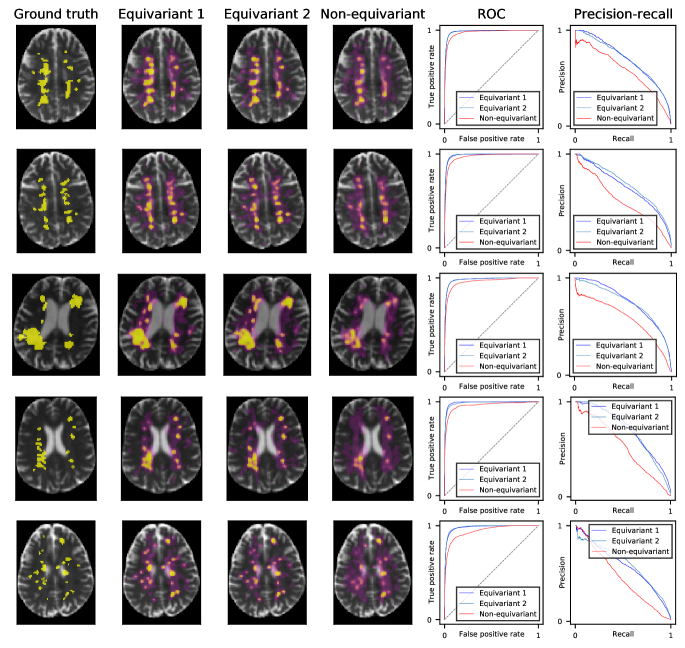
Figure 5: Segmentation of multiple-sclerosis lesions in five scans from the validation set. (a) Ground truth of one example slice per scan, (b) predictions for that slice using l_TP1_1+4 (the best equivariant model in terms of Avg-Prec and Dice score on the entire validation set), (c) predictions for that slice using l_TP1_1+3 (the best equivariant model in terms of AUC on the entire validation set), (d) predictions for that slice using the best non-rotation-equivariant model (n_4), (e) ROC curves of all models on the full scans, (f) precision-recall curves of all models on the full scans. While the equivariant models are very certain (yellow areas) at most positions, the non-rotation-equivariant model has large areas of high uncertainty (purple areas).

Figure 5 shows the segmentation of six validation samples by presenting one example slice per scan with its ground truth and the predictions from two equivariant models, the best using late and the best using gradual $q$-reduction, and from the best non-rotation-equivariant model. Additionally, it shows the ROC and precision-recall curves of the models. While all models roughly predict the ground truth, the equivariant models predict it more accurately. It can especially be seen that while the equivariant models predict the MS lesions with high confidence and have very small values outside the areas around the lesions, the non-rotation-equivariant model is very uncertain at many positions. This also explains the low AvgPrec scores of the non-rotation-equivariant models.

Figure 6: Comparison of average precision (AvgPrec) scores of equivariant models (blue) and non-rotation-equivariant models (red) in relation to their number of parameters. The two non-rotation-equivariant models with more parameters (but similar feature map sizes) as the equivariant models perform much worse than the non-rotation-equivariant models with much fewer parameters. All shown equivariant models generalize better than the non-rotation-equivariant models. As many equivariant models, including the best ones, have more parameters than the best non-rotation-equivariant models, the equivariance introduces a quality improvement that cannot only be explained by a reduction of the number of parameters. Instead, the equivariance allows the use of many parameters that can effectively capture the essence of the dataset so that the model does not underfit while still restricting it so that overfitting is effectively reduced without using additional regularization.

Figure 6 compares the performance (AvgPrec) of the equivariant models and the non-rotation-equivariant models in relation to their number of parameters. The non-rotation-equivariant models with fewer parameters perform much better than the non-rotation-equivariant models with more parameters but similar feature map sizes as the equivariant models. But as many equivariant models, including the best ones, have more parameters than the best non-rotation-equivariant models, the superiority of the equivariant models cannot (only) be explained by a reduction of the number of parameters. The absolute and relative differences between the training and validation results of most equivariant models are much larger than for the non-rotation-equivariant models, indicating that the proposed equivariant layer introduces some regularization. But there are also effects beside regularization that enable the equivariant models to achieve better results, as most equivariant models, including the best ones, outperform the non-rotation-equivariant models in the training metrics as well.

Behaviour on Reduced Training Dataset

(a)

(b)

(c)

Figure 7: Comparison of the best equivariant model with the best non-rotation-equivariant model both trained on reduced subsets of the training set. The plots show the AUC scores (left), AvgPrec scores (middle), and Dice scores (right) of our best equivariant model, l_TP1_1+4,, (blue) and the best non-rotation-equivariant model, n_4, (red) trained on reduced subsets where the subset size ($x$-axis) is described relative to the full training set size. The scores are measured on the full validation set. Our equivariant model trained on only $26\%$ of the training scans achieves more than $100\%$ of the AUC score, $97.6\%$ of the AvgPrec score, and $97.0\%$ of the Dice score of the non-rotation-equivariant model trained on the full dataset. When trained on $66\%$ of the training scans, our equivariant model outperforms the non-rotation-equivariant model trained on the full training set by $1.9\%$ in AUC score, by $24.7\%$ in AvgPrec score, and by $15.0\%$ in Dice score. Therefore, equivariant methods generalize better and thus require smaller training sets, as expected. Moreover, when matching the training set size for both methods, the equivariant method performs better in almost all cases, and never considerably worse.

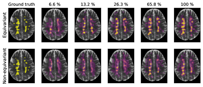
Figure 8: Segmentation of multiple-sclerosis lesions in one scan from the validation set using an equivariant and a non-rotation-equivariant model both trained on reduced subsets of the training set. From left to right, we show the ground truth segmentation and predictions using our best equivariant model, l_TP1_1+4, (top) and the best non-rotation-equivariant model, n_4, (bottom) trained on $6.6\%$, $13.2\%$, $26.3\%$, $65.8\%$, and $100\%$ of the training scans. While the equivariant model already achieves quite accurate segmentations with $26.3\%$ of the training samples, the segmentations of the non-rotation-equivariant model only start getting accurate with $65.8\%$ of the training samples, which also indicates that our equivariant model generalizes faster.

In order to analyze their generalization capabilities, we trained our best (measured in AvgPrec and Dice score) equivariant model and the best non-rotation-equivariant model on reduced subsets of the training set and found that the equivariant model outperforms the non-rotation-equivariant model in almost all subset sizes. Figure 7 shows the AUC, AvgPrec, and Dice scores of both models on different subset sizes. Our model trained on only $26\%$ of the training scans achieves $100.1\%$ of the AUC score, $97.6\%$ of the AvgPrec score, and $97.0\%$ of the Dice score of the non-rotation-equivariant model trained on the full training dataset. When trained on $66\%$ of the training scans, our equivariant model outperforms the non-rotation-equivariant model trained on the full training set by $1.9\%$ in AUC score, by $24.7\%$ in AvgPrec score, and by $15.0\%$ in Dice score. This enables to use smaller datasets while achieving the same or better performance. Moreover, when matching the training set size for both methods, the equivariant method performs better in almost all cases, and never considerably worse. Figure 8 confirms these results by comparing the segmentation of one example slice using the equivariant and the non-rotation-equivariant models trained on different subset sizes.

Comparison of $q$-Reduction Strategies, Basis Filters, Layers, Channel Setups, and Radial Basis Functions

Models using late $q$-reduction perform much better than models using gradual $q$-reduction. The TP$\pm 1$ basis outperforms all other proposed filter bases. For late $q$-reduction models, the best results are achieved using one $pq$-layer and three or four $p$-layers. For gradual $q$-reduction models, one $pq$-layer with either one or two $p$-layers works best. Small changes to the number of channels do not influence the results much. Also using order $l=2$ and $l=3$ channels neither leads to much better nor much worse performance. The best results could be achieved with a radial basis that consists of a FC network applied to cosine radial basis functions (cosine+fc). While using Gaussian+fc also works quite well, models using no FC network in the radial basis (cosine, Gaussian) perform much worse.

Training Times and Memory Consumption

The equivariant models trained about $0.5-2.5$ days until convergence and required about $12-24$ GB of GPU RAM while most non-rotation-equivariant models trained only a few hours until convergence and only required $<2$ GB of GPU memory.

The long training times of the equivariant models are caused by i) more epochs until convergence, ii) computation of the kernel after each weight update, and iii) longer backpropagation chains to the kernel parameters (because the kernel does not consist of the parameters but is computed based on functions of the parameters). The first reason seems to have less relevance, as models with smaller feature maps but more epochs until convergence were faster than models with larger feature maps but fewer epochs. As the kernels in the $pq$-layers are much larger than in the $p$-layers, the training times mostly depend on the number of $pq$-layers and their number of channels.

The GPU RAM consumption was mainly caused by the feature maps stored during the forward pass and their gradients computed during the backward pass, which is why the models with late $q$-reduction required much more memory (up to $24$ GB) than the models with gradual $q$-reduction (up to $16$ GB). The difference in memory consumption between the equivariant and the reference models is caused by i) the precomputed parts of the kernels, ii) the intermediate values stored during kernel computation to be used in the backward pass, and iii) the gated nonlinearities requiring to store more intermediate feature maps.

6 Conclusions

In this work, we proposed $\mathrm{SE}(3)$-equivariant deep learning for diffusion MRI data and showed that it yields better results and decreases the required number of training samples.

The superiority of the equivariant approach over non-rotation-equivariant models may be explained by the restrictions it imposes on the filters. As the non-rotation-equivariant models use unrestricted convolutional kernels, they need to learn the rotational equivariance from data. This means that their parameters need to capture the equivariance and all other information contained in the dataset, whereas the parameters of the equivariant models do not need to capture the equivariance as it is already imposed by the model itself. Thus the parameters of equivariant models can be used more effectively for capturing all other aspects of the data. This prevents underfitting and simplifies training. Another drawback of the non-rotation-equivariant models is that they may overfit on specific orientations in the training set, while the rotational equivariance of the proposed models prevents this. In the validation set, the non-rotation-equivariant models cannot recognize orientations of patterns not seen during training, while the equivariant models recognize these patterns and thus achieve better results.

This can also explain why the equivariant models require a smaller number of training samples. When trained on only very few samples, this benefit might become less relevant compared to overfitting on other properties of the patterns not related to rotational equivariance, explaining why then the equivaviant and non-rotation-equivariant models perform similarly on tiny training sets, e.g. the patterns in different scans may also differ in scale or brightness, they may be deformed or some types of patterns may only be present in some samples.

There may be several reasons why the late $q$-reduction strategy outperforms the gradual one: Using a different $q$-sampling scheme in the output of a layer than in the input may require interpolations that may be hard to learn for the layer. Additionally, the late $q$-reduction layer, q-length weighted average, operates point-wise in $p$-space, whereas in gradual $q$-reduction, a filtering layer with a $p$-space kernel size greater than one is used, which may be harder to train. In order to achieve the same total receptive field, gradual $q$-reduction requires less layers than late $q$-reduction, because of the larger kernel size of its $q$-reduction layer compared to the point-wise late $q$-reduction layer. This can explain why the best late $q$-reduction models have more $p$-layers than the best gradual models.

The reason for the TP$\pm 1$ filter basis performing best may be that it can access more aspects of the structural dependencies between $p$- and $q$-space than the other proposed bases, as explained in Section 3.2.6. Another reason of its success may be that it has more capacity, noticeable by the larger number of parameters. From the results it may also be concluded that fine angular details detected by higher-order filters do not seem to have much relevance, as using higher-order filters does not lead to better performance. The benefit of using fully connected (FC) networks with the radial basis functions may be explained by their larger capacity, which allows them to better detect radial patterns.

In general, the equivariance of the proposed layer allows the use of many parameters that can effectively capture the essence of the dataset, so that the model does not underfit while still restricting it so that overfitting is effectively reduced without using additional regularization like data augmentation. Our results show that using the proposed equivariant layer can help increasing the performance of predictions on dMRI scans, thus future research in this direction seems promising. Besides applying the proposed equivariant network architecture to different datasets and tasks, also different architectures including the proposed layer may be developed, e.g. architectures with equivariant $p$-space pooling. As the proposed layer supports vector and tensor inputs and outputs, also architectures predicting vectors, e.g. for fiber detection, or with diffusion tensors as input or outputs may be built (see Appendix C).

While the derivation of the layers is mathematically involved, our public implementation can be easily used out of the box without understanding the mathematical background, and gives immediate access to the benefits of equivariant deep learning for diffusion MRI. Merely general practices are advisable such as tuning the learning rate.

Acknowledgments

This work was supported by the Munich Center for Machine Learning (Grant No. 01IS18036B) and the BMBF project MLwin.

Appendix A Theoretical Background

A.1 Groups, Group Representations, and Equivariance

Intuitively, a group $G$ may be seen as a finite or infinite set of invertible and composable operations acting on some set $\mathcal{X}$. Examples of groups are the translations in 3D, the rotations in 3D, denoted by $\mathrm{SO}(3)$, and the roto-translations in 3D, denoted by $\mathrm{SE}(3)$. For a detailed formal introduction to groups, see for example Shapira (2019); Löh (2017); Rotman (1995).

If $\mathcal{X}$ is a vector space, then a group $G$ can act on $\mathcal{X}$ through a (group) representation $\bm{D}^{\mathcal{X}}$, which is defined as a function from $G$ to the set of invertible linear transformations (or invertible square matrices) on $\mathcal{X}$ with the following property (Hall, 2015; Procesi, 2007; Thomas et al., 2018):

$$\bm{D}^{\mathcal{X}}_{g}\circ\bm{D}^{\mathcal{X}}_{h}=\bm{D}^{\mathcal{X}}_{g\cdot h}\qquad\forall g,h\in G,$$ (27)

where $\bm{D}^{\mathcal{X}}_{g}$ denotes the representation $\bm{D}^{\mathcal{X}}$ applied to $g\in G$ and is called a representation of the group element $g$ on $\mathcal{X}$, the operator “$\circ$” denotes function composition, and “$\cdot$” denotes composition of group elements (group multiplication).

Now consider a function $f\colon\mathcal{X}\to\mathcal{Y}$ mapping between the vector spaces $\mathcal{X}$ and $\mathcal{Y}$. Given a group $G$ and two representations $\bm{D}^{\mathcal{X}}$, $\bm{D}^{\mathcal{Y}}$ of $G$ acting on $\mathcal{X}$ and $\mathcal{Y}$, respectively, the function $f$ is called equivariant under $G$ if the following holds (Hall, 2015; Procesi, 2007; Thomas et al., 2018):

$$f\left(\bm{D}^{\mathcal{X}}_{g}[\bm{x}]\right)=\bm{D}^{\mathcal{Y}}_{g}\left[f(\bm{x})\right]\qquad\forall g\in G\qquad\forall\bm{x}\in\mathcal{X}.$$ (28)

Intuitively, equivariance means that if the input of $f$ is transformed by some group element $g$ then this leads to the same results as applying $f$ to the non-transformed input and transforming the output of $f$ by $g$. Thus, rotation-equivariant neural networks produce the same segmentation results (up to rotation) regardless of how the input image is rotated.

If $f$ is equivariant and $\bm{D}^{\mathcal{Y}}_{g}$ is the identity for all $g\in G$, then $f$ is said to be invariant under $G$ (Procesi, 2007; Thomas et al., 2018). Invariance means that the output of $f$ does not change if its input is transformed by some $g\in G$. Thus, rotation-equivariant neural networks produce the same image-classification results (not rotatable) regardless of how the input image is rotated.

For a group $G$ there may be multiple different representations on the same vector space $\mathcal{X}$ (Procesi, 2007; Beveren, 2012). A representation $\bm{D}^{\mathcal{X}}$ of $G$ on $\mathcal{X}$ is called reducible if there exists a basis transformation in $\mathcal{X}$, described by the invertible square-matrix $\bm{Q}$, such that the representation in the new basis, $\bm{Q}^{-1}\bm{D}^{\mathcal{X}}_{g}\bm{Q}$, is a block-diagonal matrix, i.e. whose blocks $\bm{D}^{\mathcal{X}_{i}}_{g}$ act on subspaces $\mathcal{X}_{i}$, with the conditions that $\mathcal{X}$ is the direct sum of all $\mathcal{X}_{i}$ and that each $\mathcal{X}_{i}$ is closed under the corresponding representation $\bm{D}^{\mathcal{X}_{i}}_{g}$, i.e. $\bm{D}^{\mathcal{X}_{i}}_{g}\bm{x}_{i}\in\mathcal{X}_{i}\;\forall g\in G\;\forall\bm{x}_{i}\in\mathcal{X}_{i}.$ The intuition behind $\bm{Q}^{-1}\bm{D}^{\mathcal{X}}_{g}\bm{Q}$ is that the linear operator $\bm{D}^{\mathcal{X}}_{g}$ is applied in a different basis, i.e. $\bm{Q}^{-1}\bm{D}^{\mathcal{X}}_{g}\bm{Q}y$ means: map $y$ to basis of $\bm{D}^{\mathcal{X}}_{g}$ using $\bm{Q}$, apply $\bm{D}^{\mathcal{X}}_{g}$, map it back to basis of $y$ using $\bm{Q}^{-1}$. A representation that cannot be decomposed in such a way is called an irreducible representation or irrep.

A.2 Spherical Tensors and Related Concepts

Tensors are quantities transforming under rotations in a very specific way depending on their order $l\in\mathbb{N}_{0}$, and which in 3D can be described using $3^{l}$ components, which in the case of real tensors are real numbers. For the purposes of this work (i.e. considering only contravariant, real 3D tensors), a tensor $\bm{T}$ of order $l$ transforms under the rotation $g\in\mathrm{SO}(3)$ into the tensor $\bm{T}^{\prime}$ (of same order $l$) as follows (Hess, 2015; Dubbers & Stöckmann, 2013):

$$T_{\mu_{1},\mu_{2}\dots\mu_{l}}^{\prime}=\sum_{\nu_{1},\nu_{2}\dots\nu_{l}}(\mathcal{R}_{g})_{\mu_{1},\nu_{1}}(\mathcal{R}_{g})_{\mu_{2},\nu_{2}}\dots(\mathcal{R}_{g})_{\mu_{l},\nu_{l}}T_{\nu_{1},\nu_{2}\dots\nu_{l}},$$ (29)

where $\mu_{1},\mu_{2}\dots\mu_{l},\nu_{1},\nu_{2}\dots\nu_{l}$ are indices with values $1,2,3$ used to access the components of the tensors and $\bm{\mathcal{R}}_{g}$ is the rotation matrix of $g$. Scalars are tensors of order $l=0$ and do not transform under rotations, whereas vectors are tensors of order $l=1$.

A.2.1 Spherical Tensors, Spherical Harmonics, and Wigner D-Matrices

The tensors described so far are called Cartesian tensors. Although these tensors obey the simple transformation rule of Eq. (29), they may be reducible w.r.t. rotations, meaning that they can be decomposed into other possibly lower-order tensors, whose components can be computed as linear combinations of the original tensor components, and the resulting tensors can be rotated independently (Brouder et al., 2008; Man, 2013). Tensors can instead be represented in a different basis, the spherical basis, in which they are always irreducible. Such tensors are called spherical tensors and their components are called spherical components (Hess, 2015; Brouder et al., 2008; Man, 2013; Reisert & Burkhardt, 2009; Biedenharn & Louck, 1984). Under the rotation $g\in\mathrm{SO}(3)$, a spherical tensor $\bm{\mathcal{T}}^{(l)}$ of order $l$ transforms into $\bm{\mathcal{T}}^{\prime(l)}$ using the irreducible representations of $\mathrm{SO}(3)$ as follows (Blanco et al., 1997):

$$\bm{\mathcal{T}}^{\prime(l)}=\bm{D}^{(l)}_{g^{-1}}\bm{\mathcal{T}}^{(l)},$$ (30)

where $\bm{D}^{(l)}_{g^{-}1}$, called (real) Wigner D-matrix of order $l$, is an irreducible representation of $g^{-1}$ and is orthogonal.

Spherical tensors of order $l$ can be described using $2l+1$ either complex or real components. Describing them using the same number of either complex or real components is possible due to symmetries of spherical tensors (Man, 2013; Reisert & Burkhardt, 2009; Blanco et al., 1997). As real numbers require less memory for storage and are more efficient from a computational point of view (Reisert & Burkhardt, 2009), we prefer to use real components and denote the vector space of (the real-valued description of) order $l$ spherical tensors by $\mathcal{S}^{(l)}$.

For the cases of $l=0$ (scalars) and $l=1$ (vectors), the (real) Wigner D-matrices are (up to a reordering of its components in the case of $l=1$) given by $D^{(0)}_{g}=1$ and $\bm{D}^{(1)}_{g}=\bm{\mathcal{R}}_{g}$ (Blanco et al., 1997; Reisert & Burkhardt, 2009; Biedenharn & Louck, 1984; Thomas et al., 2018).

There is a special set of functions mapping points on the sphere $S^{2}$ to spherical tensors, the (real) spherical harmonics $\bm{Y}^{(l)}$, where $l$ denotes the order of the spherical harmonics and is equal to the order of its outputs.

Under a rotation $g\in\mathrm{SO}(3)$, the (real) spherical harmonics transform like spherical tensors using the (real) Wigner D-matrices (Blanco et al., 1997; Biedenharn & Louck, 1984; Thomas et al., 2018):

$$\left(g\bm{Y}^{(l)}\right)(\bm{n})=\bm{Y}^{(l)}\left(\bm{\mathcal{R}}_{g^{-1}}\bm{n}\right)=\bm{D}^{(l)}_{g^{-1}}\left[\bm{Y}^{(l)}(\bm{n})\right],$$ (31)

where $\bm{n}$ is a unit vector in $\mathbb{R}^{3}$ representing a point on the sphere, meaning $\bm{n}\in S^{2}$.

For the case $l=0$ it holds that $\bm{Y}^{(0)}(\bm{n})=\mathrm{const.}$, while for $l=1$ it holds (up to a reordering of the components of $\bm{n}$) that $\bm{Y}^{(1)}(\bm{n})=c\bm{n}$ with some constant factor $c\in\mathbb{R}$ (Blanco et al., 1997; Thomas et al., 2018).

A.2.2 Tensor Product and Clebsch–Gordan Coefficients

Two spherical tensors $\bm{\mathcal{T}}^{(l_{1})}$, $\bm{\mathcal{U}}^{(l_{2})}$ of orders $l_{1},l_{2}$ can be coupled using the tensor product, denoted by $\otimes$, which for spherical tensors results in the following direct sum (concatenation) of spherical tensors (Dubbers & Stöckmann, 2013; Brouder et al., 2008; Man, 2013; Devanathan, 2002; Biedenharn & Louck, 1984; Thomas et al., 2018; Kondor, 2018):

$$\bm{\mathcal{T}}^{(l_{1})}\otimes\bm{\mathcal{U}}^{(l_{2})}\coloneqq\bigoplus_{l=|l_{1}-l_{2}|}^{l_{1}+l_{2}}\left(\bm{\mathcal{T}}^{(l_{1})}\otimes\bm{\mathcal{U}}^{(l_{2})}\right)^{(l)},$$ (32)

where $\bigoplus$ denotes the direct sum, and with

$$\left(\bm{\mathcal{T}}^{(l_{1})}\otimes\bm{\mathcal{U}}^{(l_{2})}\right)^{(l)}_{m}=\sum_{m_{1}=-l_{1}}^{l_{1}}\sum_{m_{2}=-l_{2}}^{l_{2}}C^{(l,m)}_{(l_{1},m_{1})(l_{2},m_{2})}\mathcal{T}^{(l_{1})}_{m_{1}}\mathcal{U}^{(l_{2})}_{m_{2}},$$ (33)

where $C^{(l,m)}_{(l_{1},m_{1})(l_{2},m_{2})}$ are predefined scalars, the so-called (real) Clebsch–Gordan coefficients, $l$ is the order of the resulting tensor, and $m$ with $-l\leq m\leq l$ is used to index its components. The meaningful orders $l$ of tensors resulting from the tensor product follow from the fact that the Clebsch–Gordan coefficients are only non-zero if the following holds:

$$|l_{1}-l_{2}|\leq l\leq l_{1}+l_{2},$$ (34)

and as such the tensors of other orders are zero. Additionally, it needs to hold that $m=m_{1}+m_{2}$ for the Clebsch–Gordan coefficients to be non-zero. As the values of the spherical harmonics are spherical tensors, spherical harmonics can be coupled with spherical tensors via a tensor product in the same way.

An important property of the tensor product between two spherical tensors is that it is equivariant under rotations, meaning that the resulting spherical tensors, as defined in Eq. (33), transform as follows (Reisert & Burkhardt, 2009; Thomas et al., 2018):

$$\left(\bm{D}^{(l_{1})}_{g}\bm{\mathcal{P}}^{(l_{1})}\otimes\bm{D}^{(l_{2})}_{g}\bm{\mathcal{Q}}^{(l_{2})}\right)^{(l)}=\bm{D}^{(l)}_{g}\left(\bm{\mathcal{P}}^{(l_{1})}\otimes\bm{\mathcal{Q}}^{(l_{2})}\right)^{(l)}\qquad\forall g\in\mathrm{SO}(3),$$ (35)

where $\bm{D}$ are the Wigner D-matrices. For some special values of $(l_{1},l_{2},l)$, the tensor product of spherical tensors is related to some well-known operations: The case of $(0,0,0)$ is equal to normal multiplication of two scalars, $(0,1,1)$ and $(1,0,1)$ are equal to scalar multiplication of a vector, while the cases $(1,1,0)$ and $(1,1,1)$ are proportional to the dot product and the cross product of two vectors, respectively (Dubbers & Stöckmann, 2013; Devanathan, 2002; Abramowitz & Stegun, 1972; Thomas et al., 2018).

A.2.3 Multi-Channel Spherical Tensors and Spherical-Tensor Fields

So far spherical tensors have been defined with a single order $l$. Following Kondor (2018), multiple such spherical tensors can be combined using the direct sum (concatenation), denoted by $\bigoplus$. We will call such objects multi-channel spherical tensors and call the spherical tensors comprising it channels. This is related to the channels in convolutional neural networks, where every pixel/voxel has scalar channels, but the concept of channels is generalized from scalars to other tensors as e.g. done in Thomas et al. (2018); Kondor (2018). The type of the multi-channel spherical tensor is defined by the tuple $\bm{\tau}=(\tau_{0},\tau_{1},\dots)$ where each $\tau_{l}\in\mathbb{N}_{0}$ defines the number of channels of order $l$. The space of multi-channel spherical tensors of type $\bm{\tau}$ thus is defined as $\mathcal{S}^{\bm{\tau}}:=\bigoplus_{l=0}^{\infty}\bigoplus_{c^{(l)}=1}^{\tau_{l}}\mathcal{S}^{(l)}$, where $c^{(l)}$ is used to index the channels of order $l$, and $\mathcal{S}^{(l)}$ is the vector space of spherical tensors of order $l$. The total number $C$ of channels is $C=\sum_{l=0}^{\infty}\tau_{l}$. In this work, the channel is often directly indexed using $c\in\{1,\dots,C\}$ and the order of this channel may be denoted by $l(c)$.

A 3D (multi-channel) spherical-tensor field $\bm{I}$ of type $\bm{\tau}$ assigns a type-$\bm{\tau}$ spherical tensor to every position in space, i.e. $\bm{I}\colon\mathbb{R}^{3}\to\mathcal{S}^{\bm{\tau}}$. Such a tensor field has special transformation properties under rotations and translations (Hess, 2015; Reisert & Burkhardt, 2009; Weiler et al., 2018b):

$$(g,\mathcal{T}_{\bm{t}})[\bm{I}](\bm{x})=\bm{D}^{\bm{\tau}}_{g}\bm{I}\left(\mathcal{\bm{R}}_{g^{-1}}(\bm{x}-\bm{t})\right)\qquad\forall\bm{x}\in\mathbb{R}^{3},$$ (36)

where $(g,\mathcal{T}_{\bm{t}})\in\mathrm{SE}(3)$ is a roto-translation with rotation $g\in\mathrm{SO}(3)$ followed by translation $\bm{t}\in\mathbb{R}^{3}$, with the multi-channel Wigner D-matrix $\bm{D}^{\bm{\tau}}_{g}$ of type $\bm{\tau}$, and with the rotation matrix $\mathcal{\bm{R}}_{g^{-1}}$ of the inverse rotation $g^{-1}$. This means that the value for position $\bm{x}$ of the transformed tensor field is read from the original position (before the transformation) given by $\mathcal{\bm{R}}_{g^{-1}}(\bm{x}-\bm{t})$. Additionally, the resulting spherical tensor is transformed according to the rotation $g$ using $\bm{D}^{\bm{\tau}}_{g}$. Note that the latter transformation does not depend on the translation. The matrix $\bm{D}^{\bm{\tau}}_{g}$ can be built as direct sum of Wigner D-matrices $\bm{D}^{(l)}_{g}$, i.e. $\bm{D}^{\bm{\tau}}_{g}:=\bigoplus_{l=0}^{\infty}\bigoplus_{c^{(l)}=1}^{\tau_{l}}\bm{D}^{(l)}_{g}$. This means that each channel transforms independently but the tensor components within each channel influence each other during transformation. If for example the tensor field represents a 3D MR image with three contrasts ($T_{1}$, $T_{2}$, proton density), then it would contain three scalar channels (the contrasts) but no vector channels, as each of the channels transforms independently whereas the three parts of a vector channel would influence each other during transformation because they jointly express directions in the 3D image space (Weiler et al., 2018b; Kondor, 2018).

Appendix B Implementation Details

B.1 Radial Basis Functions

B.1.1 Gaussian Radial Basis Functions as used in Weiler et al. (2018b)

A set of Gaussian radial basis functions can be defined as

$$\varphi_{\text{Gaussian}}^{(k)}(x)\coloneqq\text{exp}\left(-\frac{(x-\mu_{k})^{2}}{2\sigma^{2}}\right)$$ (37)

with (predefined or learned) means $\mu_{k}$ and (predefined or learned) variance $\sigma^{2}$, where $k$ identifies each function in the set and has values from $1$ to the radial basis size $K$.

B.1.2 Cosine Radial Basis Functions as used in Geiger et al. (2020)

A set of cosine radial basis functions can be defined as

$$\varphi_{\text{cos}}^{(k)}(x)\coloneqq\begin{cases}\cos^{2}(\gamma(x-\mu_{k})\frac{\pi}{2})&1\geq\gamma(x-\mu_{k})\geq-1\\ 0&\mathrm{otherwise}\end{cases}$$ (38)

with (predefined or learned) reference points $\mu_{k}$ and (predefined) normalization factor $\gamma$, where $k$ identifies each function in the set and has values from $1$ to the radial basis size $K$.

B.1.3 Fully Connected Neural Network applied to Radial Basis Functions as used in Thomas et al. (2018); Geiger et al. (2020)

First some set of radial basis functions $\varphi^{\prime(i)}$ is applied to the input $x$. The the output of each radial basis function in this set is then treated as input neuron to a fully connected neural network. The radial basis size $K$ defines the number of neurons of the output layer of that network, while the number of hidden layers and neurons in these layers are hyperparameters. In the case of a two-layer network, the radial basis function is defined as:

$$\varphi_{\text{NN}}^{(k)}(x)\coloneqq b_{k}^{(2)}+\sum_{j}W_{k,j}^{(2)}\text{ReLU}\left(b_{j}^{(1)}+\sum_{i}W_{j,i}^{(1)}\varphi^{\prime(i)}(x)\right),$$ (39)

where $\bm{W}^{(2)}$, $\bm{W}^{(1)}$, $\bm{b}^{(2)}$, and $\bm{b}^{(1)}$ are learned parameters, $j$ and $i$ are indices of the hidden respectively input layer, and $\varphi^{\prime(i)}$ is some set of radial basis functions.

B.2 Equivariant Nonlinearities

When using spherical-tensor fields (see Appendix A.2.3) as feature maps like used in the layer proposed in Eq. (8), elementwise nonlinearities like ReLU are in general not equivariant under rotations (Weiler et al., 2018b). Instead special nonlinearities like tensor product nonlinearities (Kondor, 2018), norm-nonlinearities (Worrall et al., 2016), squashing nonlinearities (Sabour et al., 2017), or gated nonlinearities (Weiler et al., 2018b) are required.

Note that as scalars are invariant under rotations, elementwise nonlinearities (like ReLU) can be used for $l=0$ channels (Weiler et al., 2018b).

B.3 Discretization

Discretized Feature Maps

The layer definition (8) assumes feature maps over the space $\mathbb{R}^{3}\oplus\mathbb{R}^{3}$ and these feature maps would require infinite memory. Thus, in practice, feature maps are discretized using sampling schemes. In this work, the sampling schemes used in dMRI scans are also used for the feature maps, so the $p$-space is sampled on a finite Cartesian 3D grid, while the $q$-space uses a predefined, not necessarrily regular, finite sampling scheme.

This means that the discretized $p$-space has the form:

$$\mathcal{P}\coloneqq\mathcal{P}_{x}\times\mathcal{P}_{y}\times\mathcal{P}_{z}\subset\mathbb{Z}^{3}\subset\mathbb{R}^{3},$$ (40)

with $\mathcal{P}_{x}=\{1,\dots,P_{x}\}$, $\mathcal{P}_{y}=\{1,\dots,P_{y}\}$, and $\mathcal{P}_{z}=\{1,\dots,P_{z}\}$, where $P_{x},P_{y},P_{z}$ are the sizes of the $p$-space voxel grid of the feature map.

The discretized $q$-space is the finite set

$$\mathcal{Q}\coloneqq\{\bm{q}_{n}\}_{n=1}^{Q}\subset\mathbb{R}^{3},$$ (41)

consisting of the $Q$ predefined $q$-vectors $\bm{q}_{n}\in\mathbb{R}^{3}$ where $Q$ and the $\bm{q}_{n}$ may be different for feature maps of different layers. While $\mathcal{Q}$ for the input, denoted by $\mathcal{Q}_{\mathrm{in}}$, is dictated by the input data structure, e.g. the output of the previous layer or the input to the network, $\mathcal{Q}$ for the output, denoted by $\mathcal{Q}_{\mathrm{out}}$, is a freely choosable hyperparameter. This means that we can choose $Q_{\mathrm{out}}=1$ to “collapse” $q$-space in some layer. This may for example be used for image segmentation (one prediction for each $p$-space coordinate) or image classification (where $p$-space gets “collapsed” as well, namely through pooling). Note that $\mathcal{Q}_{\mathrm{out}}={(0,0,0)}$ is required to achieve equivariance under rotations in $q$-space, as the $q$-space coordinate offsets used in the angular and radial basis are not rotation equviariant for other $\mathcal{Q}_{\mathrm{out}}$. For invariance under rotations in $q$-space, only scalar ($l_{\mathrm{out}}=0$) output channels must be used, at least in the final layer.

Using these definitions, a discretized feature map $\hat{\bm{I}}$ of type $\bm{\tau}$ can be defined as

$$\hat{\bm{I}}\colon\mathcal{P}\oplus\mathcal{Q}\to\mathcal{S}^{\bm{\tau}},$$ (42)

which can be represented using an array of size

$$\dim\left(\mathcal{S}^{\bm{\tau}}\right)\times P_{z}\times P_{y}\times P_{x}\times Q.$$ (43)

Discretized Convolutional Layer

A layer $\hat{\mathcal{L}}$ working on these discretized feature maps is a function of the form

$$\hat{\mathcal{L}}\colon(\mathcal{P}_{\mathrm{in}}\oplus\mathcal{Q}_{\mathrm{in}}\to\mathcal{S}^{\bm{\tau}_{\mathrm{in}}}) \to(\mathcal{P}_{\mathrm{out}}\oplus\mathcal{Q}_{\mathrm{out}}\to\mathcal{S}^{\bm{\tau}_{\mathrm{out}}}),$$ (44)

where $\mathcal{P}_{\mathrm{in}}$, $\mathcal{Q}_{\mathrm{in}}$, and $\mathcal{S}^{\bm{\tau}_{\mathrm{in}}}$ are the $p$-space, $q$-space, and spherical tensor space of the input feature map, respectively, and $\mathcal{P}_{\mathrm{out}}$, $\mathcal{Q}_{\mathrm{out}}$, and $\mathcal{S}^{\bm{\tau}_{\mathrm{out}}}$ those of the output feature map.

This layer $\hat{\mathcal{L}}$ can be defined analogously to $\mathcal{L}$ (8) by replacing the sum of $\bm{p}_{\mathrm{in}}$ and $\bm{q}_{\mathrm{in}}$ over $\mathbb{R}^{3}$ by sums over $\mathcal{P}_{\mathrm{in}}$, the discretized input $p$-space, and $\mathcal{Q}_{\mathrm{in}}$, the discretized input $q$-space:

$$\begin{split}\hat{\mathcal{L}}_{m_{\mathrm{out}}}^{(c_{\mathrm{out}})}[\hat{\bm{I}}](\bm{p}_{\mathrm{out}},\bm{q}_{n_{\mathrm{out}}})\coloneqq&\sum_{c_{\mathrm{in}},c_{\mathrm{filter}},k}W_{c_{\mathrm{in}},c_{\mathrm{filter}},c_{\mathrm{out}},k}\sum_{\begin{subarray}{c}m_{\mathrm{filter}}\in\{-l_{\mathrm{filter}},\dots,l_{\mathrm{filter}}\},\\ m_{\mathrm{in}}\in\{-l_{\mathrm{in}},\dots,l_{\mathrm{in}}\}\end{subarray}}C_{(l_{\mathrm{filter}},m_{\mathrm{filter}})(l_{\mathrm{in}},m_{\mathrm{in}})}^{(l_{\mathrm{out}},m_{\mathrm{out}})}\\ &\qquad\times\sum_{\begin{subarray}{c}\bm{p}_{\mathrm{in}}\in\mathcal{P}_{\mathrm{in}},\\ \bm{q}_{n_{\mathrm{in}}}\in\mathcal{Q}_{\mathrm{in}}\end{subarray}}F_{m_{\mathrm{filter}}}^{(c_{\mathrm{filter}},k)}(\bm{p}_{\mathrm{out}}-\bm{p}_{\mathrm{in}},\bm{q}_{n_{\mathrm{out}}},\bm{q}_{n_{\mathrm{in}}})\hat{I}_{m_{\mathrm{in}}}^{(c_{\mathrm{in}})}(\bm{p}_{\mathrm{in}},\bm{q}_{n_{\mathrm{in}}}).\end{split}$$ (45)

Eq. (45) can be rewritten as follows:

$$\begin{split}\hat{\mathcal{L}}_{m_{\mathrm{out}}}^{(c_{\mathrm{out}})}[\hat{\bm{I}}](\bm{p}_{\mathrm{out}},\bm{q}_{n_{\mathrm{out}}})=&\sum_{c_{\mathrm{in}},c_{\mathrm{filter}},k}W_{c_{\mathrm{in}},c_{\mathrm{filter}},c_{\mathrm{out}},k}\sum_{\begin{subarray}{c}m_{\mathrm{filter}}\in\{-l_{\mathrm{filter}},\dots,l_{\mathrm{filter}}\},\\ m_{\mathrm{in}}\in\{-l_{\mathrm{in}},\dots,l_{\mathrm{in}}\}\end{subarray}}C_{(l_{\mathrm{filter}},m_{\mathrm{filter}})(l_{\mathrm{in}},m_{\mathrm{in}})}^{(l_{\mathrm{out}},m_{\mathrm{out}})}\\ &\qquad\times\sum_{\begin{subarray}{c}\bm{p}_{\mathrm{filter}}\in\mathcal{P}_{\mathrm{filter}},\\ \bm{q}_{n_{\mathrm{in}}}\in\mathcal{Q}_{\mathrm{in}}\end{subarray}}F_{m_{\mathrm{filter}}}^{(c_{\mathrm{filter}},k)}(-\bm{p}_{\mathrm{filter}},\bm{q}_{n_{\mathrm{out}}},\bm{q}_{n_{\mathrm{in}}})\\ &\qquad\qquad\times\hat{I}_{m_{\mathrm{in}}}^{(c_{\mathrm{in}})}(\bm{p}_{\mathrm{filter}}+\bm{p}_{\mathrm{out}},\bm{q}_{n_{b}}),\\ \end{split}$$ (46)

where the $p$-space filter coordinate $\bm{p}_{\mathrm{filter}}=-\Delta\bm{p}=\bm{p}_{\mathrm{in}}-\bm{p}_{\mathrm{out}}$ is introduced, with values in the filter space $\mathcal{P}_{\mathrm{filter}}=\left\{-P_{\mathrm{filter}},\dots,0,\dots,P_{\mathrm{filter}}\right\}^{3}\subset\mathbb{Z}^{3}$, and the $p$-space filter radius $P_{\mathrm{filter}}\in\mathbb{N}_{0}$ leading to a $p$-space filter size of $2P_{\mathrm{filter}}+1$. The feature map $\hat{\bm{I}}$ is assumed to be zero for arguments outside its domain. This corresponds to defining an appropriate zero padding in a convolutional layer. Note that for Eq. (46) to hold, the radial basis filters need to be defined to be zero for $(\bm{p}_{\mathrm{in}}-\bm{p}_{\mathrm{out}})\notin\mathcal{P}_{\mathrm{filter}}$.

By rearranging the sums and introducing the kernel $\bm{K}$, containing all parameters and basis filters, which we propose to define as

$$\begin{split}K_{m_{\mathrm{out}},m_{\mathrm{in}}}^{(c_{\mathrm{out}},c_{\mathrm{in}})}(\bm{p}_{\mathrm{filter}},\bm{q}_{n_{\mathrm{out}}},\bm{q}_{n_{\mathrm{in}}})\coloneqq&\sum_{c_{\mathrm{filter}},k}W_{c_{\mathrm{in}},c_{\mathrm{filter}},c_{\mathrm{out}},k}\\ &\qquad\times\sum_{m_{\mathrm{filter}}\in\{-l_{\mathrm{filter}},\dots,l_{\mathrm{filter}}\}}C_{(l_{\mathrm{filter}},m_{\mathrm{filter}})(l_{\mathrm{in}},m_{\mathrm{in}})}^{(l_{\mathrm{out}},m_{\mathrm{out}})}\\ &\qquad\qquad\times F_{m_{\mathrm{filter}}}^{(c_{\mathrm{filter}},k)}(-\bm{p}_{\mathrm{filter}},\bm{q}_{n_{\mathrm{out}}},\bm{q}_{n_{\mathrm{in}}}),\end{split}$$ (47)

Eq. (46) can be further rewritten:

$$\begin{split}\hat{\mathcal{L}}_{m_{\mathrm{out}}}^{(c_{\mathrm{out}})}[\hat{\bm{I}}](\bm{p}_{\mathrm{out}},\bm{q}_{n_{\mathrm{out}}})=&\sum_{\begin{subarray}{c}\bm{q}_{n_{\mathrm{in}}}\in\mathcal{Q}_{\mathrm{in}},\\ c_{\mathrm{in}},\\ m_{\mathrm{in}}\in\{-l_{\mathrm{in}},\dots,l_{\mathrm{in}}\}\end{subarray}}\sum_{\bm{p}_{\mathrm{filter}}\in\mathcal{P}_{\mathrm{filter}}}\sum_{c_{\mathrm{filter}},k}W_{c_{\mathrm{in}},c_{\mathrm{filter}},c_{\mathrm{out}},k}\\ &\qquad\times\sum_{m_{\mathrm{filter}}\in\{-l_{\mathrm{filter}},\dots,l_{\mathrm{filter}}\}}C_{(l_{\mathrm{filter}},m_{\mathrm{filter}})(l_{\mathrm{in}},m_{\mathrm{in}})}^{(l_{\mathrm{out}},m_{\mathrm{out}})}\\ &\qquad\qquad\times F_{m_{\mathrm{filter}}}^{(c_{\mathrm{filter}},k)}(-\bm{p}_{\mathrm{filter}},\bm{q}_{n_{\mathrm{out}}},\bm{q}_{n_{\mathrm{in}}})\hat{I}_{m_{\mathrm{in}}}^{(c_{\mathrm{in}})}(\bm{p}_{\mathrm{filter}}+\bm{p}_{\mathrm{out}},\bm{q}_{n_{\mathrm{in}}})\\ =&\sum_{\begin{subarray}{c}\bm{q}_{n_{\mathrm{in}}}\in\mathcal{Q}_{\mathrm{in}},\\ c_{\mathrm{in}},\\ m_{\mathrm{in}}\in\{-l_{\mathrm{in}},\dots,l_{\mathrm{in}}\}\end{subarray}}\sum_{\bm{p}_{\mathrm{filter}}\in\mathcal{P}_{\mathrm{filter}}}K_{(c_{\mathrm{out}},m_{\mathrm{out}}),(c_{\mathrm{in}},m_{\mathrm{in}})}(\bm{p}_{\mathrm{filter}},\bm{q}_{n_{\mathrm{out}}},\bm{q}_{n_{\mathrm{in}}})\\ &\qquad\times\hat{I}_{m_{\mathrm{in}}}^{(c_{\mathrm{in}})}(\bm{p}_{\mathrm{filter}}+\bm{p}_{\mathrm{out}},\bm{q}_{n_{\mathrm{in}}}).\end{split}$$ (48)

The kernel $\bm{K}$ can be represented using an array of size

$$\dim\left(\mathcal{S}^{\bm{\bm{\tau}_{\mathrm{out}}}}\right)\times\dim\left(\mathcal{S}^{\bm{\bm{\tau}_{\mathrm{in}}}}\right)\times P_{\mathrm{filter}}\times P_{\mathrm{filter}}\times P_{\mathrm{filter}}\times Q_{\mathrm{out}}\times Q_{\mathrm{in}}.$$ (49)

Equivariance of Discretized Layer

For discrete feature maps, property (5) needs to be adapted as follows:

$$(g,\mathcal{T}_{\bm{t}})[\hat{\bm{I}}](\bm{p},\bm{q})=\bm{D}^{\bm{\tau}}_{g}\Phi\left(\hat{\bm{I}}\left(\mathcal{\bm{R}}_{g^{-1}}(\bm{p}-\bm{t}),\mathcal{\bm{R}}_{g^{-1}}\bm{q}\right)\right),$$ (50)

where $(g,\mathcal{T}_{\bm{t}})\in\mathrm{SE}(3)$ with $g\in\mathrm{SO}(3)$ and $\bm{t}\in\mathbb{R}^{3}$, $\bm{p}\in\mathcal{P}$, $\bm{q}\in\mathcal{Q}$, and $\Phi\colon(\mathbb{R}^{3}\oplus\mathbb{R}^{3}\to\mathcal{S}^{\bm{\tau}})\to(\mathcal{P}\oplus\mathcal{Q}\to\mathcal{S}^{\bm{\tau}})$ is an interpolation.

Note that with Eq. (50) the equivariance property (7) is not guaranteed for $\hat{\mathcal{L}}$ if the interpolation is not trivial, i.e. if $\bm{\mathcal{R}}_{g^{-1}}(\bm{p}-\bm{t})\not\in\mathcal{P}$ or $\bm{\mathcal{R}}_{g^{-1}}\bm{q}\not\in\mathcal{Q}$. So equivariance may only hold approximately.

Also, because of discretization, aliasing artifacts may occur when using high angular filter orders $l_{\mathrm{filter}}$. This means that high-order angular basis filters should not be used in filters. The maximum order depends on the filter size $P_{\mathrm{f}}$ (see Weiler et al. (2018b)).

B.4 Efficient Implementation using 3D Convolutional Layer

The layer defined in Eq. (48) can be implemented using 3D convolutional layers (with computed kernels, see below), of which deep learning frameworks like PyTorch (Paszke et al., 2019) support efficient implementations. We will denote such a 3D convolutional layer as $\text{conv}_{\text{3D}}$.

In order to be used in a $\text{conv}_{\text{3D}}$ layer, the indices $c^{\prime}_{\mathrm{out}}$ and $c^{\prime}_{\mathrm{in}}$ are introduced which allow indexing the kernel and the feature maps for all possible values of $(n_{\mathrm{out}},c_{\mathrm{out}},m_{\mathrm{out}})$ and $(n_{\mathrm{in}},c_{\mathrm{in}},m_{\mathrm{in}})$, respectively, using just single indices. Also, the feature maps are reshaped to size

$$(\dim\left(\mathcal{S}^{\bm{\tau}}\right)\cdot Q)\times P_{z}\times P_{y}\times P_{x},$$ (51)

and the kernel is reshaped to size

$$\left(Q_{\mathrm{out}}\cdot\dim\left(\mathcal{S}^{\bm{\bm{\tau}_{\mathrm{out}}}}\right)\right)\times\left(Q_{\mathrm{in}}\cdot\dim\left(\mathcal{S}^{\bm{\bm{\tau}_{\mathrm{in}}}}\right)\right)\times P_{\mathrm{filter}}\times P_{\mathrm{filter}}\times P_{\mathrm{filter}}.$$ (52)

Using the reshaped feature map and kernel, the new indices $c^{\prime}_{\mathrm{out}},c^{\prime}_{\mathrm{in}}$, and replacing $\bm{q}_{n_{\mathrm{out}}},\bm{q}_{n_{\mathrm{in}}}$ by their indices $n_{\mathrm{out}},n_{\mathrm{in}}$, Eq. (48) can be rewritten to use the $\text{conv}_{\text{3D}}$ layer:

$$\begin{split}\hat{\mathcal{L}}_{c^{\prime}_{\mathrm{out}}(n_{\mathrm{out}},c_{\mathrm{out}},m_{\mathrm{out}})}[\hat{\bm{I}}](\bm{p}_{\mathrm{out}})={}&\sum_{c^{\prime}_{\mathrm{in}}}\sum_{\bm{p}_{\mathrm{filter}}\in\mathcal{P}_{\mathrm{filter}}}K_{c^{\prime}_{\mathrm{out}}(n_{\mathrm{out}},c_{\mathrm{out}},m_{\mathrm{out}}),c^{\prime}_{\mathrm{in}}(n_{\mathrm{in}},c_{\mathrm{in}},m_{\mathrm{in}})}(\bm{p}_{\mathrm{filter}})\\ &\qquad\times\hat{I}_{c^{\prime}_{\mathrm{in}}(n_{\mathrm{in}},c_{\mathrm{in}},m_{\mathrm{in}})}(\bm{p}_{\mathrm{filter}}+\bm{p}_{\mathrm{out}})\\ ={}&\left(\sum_{c^{\prime}_{\mathrm{in}}}\bm{K}_{c^{\prime}_{\mathrm{out}},c^{\prime}_{\mathrm{in}}}\star\hat{\bm{I}}_{c^{\prime}_{\mathrm{in}}}\right)(\bm{p}_{\mathrm{out}})\\ ={}&\ \text{conv}_{\text{3D}}(\bm{K},\hat{\bm{I}})_{c^{\prime}_{\mathrm{out}}}(\bm{p}_{\mathrm{out}}),\end{split}$$ (53)

where $\star$ denotes cross-correlation.

Kernel Computation

The computation of $\bm{K}$ can be split into multiple steps:

1. Precomputation of Clebsch–Gordan coefficients $\bm{C}$

2. Precomputation of angular basis $\bm{A}^{(c_{\mathrm{filter}})}$ for all $\bm{p}_{\mathrm{filter}}\in\mathcal{P}_{\mathrm{filter}}$, $\bm{q}_{n_{\mathrm{in}}}\in\mathcal{Q}_{\mathrm{in}}$, and $\bm{q}_{n_{\mathrm{out}}}\in\mathcal{Q}_{\mathrm{out}}$

3. (Pre)computation of radial basis $R^{(k)}$ for all $\bm{p}_{\mathrm{filter}}\in\mathcal{P}_{\mathrm{filter}}$, $\bm{q}_{n_{\mathrm{in}}}\in\mathcal{Q}_{\mathrm{in}}$, and $\bm{q}_{n_{\mathrm{out}}}\in\mathcal{Q}_{\mathrm{out}}$

4. Multiplication of radial and angular basis as per Eq. (11) and computation of $\bm{K}$ using learned weights $\bm{W}$ as per Eq. (47)

As the angular basis does not contain any learned parameters, steps 1 and 2 can be computed before training. Depending on the choice of radial basis function, the radial basis may or may not contain learned parameters. If it does, only the inputs to the radial basis functions can be precomputed but the radial basis is computed during training. If it does not contain learned parameters, then the whole radial basis can be precomputed. Step 4 is always computed during training.

The number of radial basis functions used in the $p$-difference radial basis (Eq. (14)) is chosen to be equal to $P_{\mathrm{filter}}$. For the $q$-in (Eq. (15)) and $q$-out (Eq. (16)) radial bases, it is equal to the number of different lengths of $q$-vectors in $\mathcal{Q}_{\mathrm{in}}$ and $\mathcal{Q}_{\mathrm{out}}$, respectively.

Our implementation can be found at https://github.com/philip-mueller/equivariant-deep-dmri

Appendix C Vectors and Higher-Order Tensors as Inputs or Outputs

As our proposed layer supports higher-order tensor inputs and outputs (e.g. vectors or order-2 tensors), it can be used to build neural networks with such inputs or outputs, e.g. networks for predicting diffusion tensors or using diffusion tensors as inputs.

For supporting vector ($l=1$) outputs, the output feature map of the output layer needs to be configured to contain a single $l=1$ channel. No further changes are required. Analogously the first layer can be configured to support vector inputs. For supporting order-2 tensor ($l=2$) outputs an additional step is required after the output layer. The layer uses spherical tensors in its feature maps, which for $l\leq 1$ (scalars and vectors) are (up to reordering) equal to Cartesian tensors but for $l>1$ are not.

In the case of $l>1$ a single Cartesian tensor can be decomposed into multiple spherical tensors. For example, an order $l=2$ Cartesian tensors can be decomposed into one $l=0$, one $l=1$, and one $l=2$ spherical tensors, corresponding to its isotropic, antisymmetric, and symmetric traceless parts, respectively (Hess, 2015; Man, 2013). From this follows that in order to predict order-2 Cartesian tensors, the output feature map of the output layer needs to contain one $l=0$, $l=1$, and $l=2$ channel each. These spherical tensors are then combined into an order-2 Cartesian tensor (independently for each position). If the predicted Cartesian tensor is known to be symmetric, then the $l=1$ spherical tensor is not required, as it represents the antisymmetric part and is zero for symmetric tensors. Analogously, for using an order-2 Cartesian tensor as input, the tensor is first decomposed into one $l=0$, one $l=1$, and one $l=2$ spherical tensors, and these are then given to the first layer.

Note that it is also possible to predict (or use as input) multiple scalars, vectors, or order-2 tensors or even a mix of different-order tensors (for each position).

Appendix D Proofs

D.1 Proof of Equivariance Property (7) for Layer Definition (8)

As each roto-translation can be built from a rotation followed by a translation (Ivancevic & Ivancevic, 2011) it is enough to prove equivariance under rotations and translations (of positions) independently.

Proof of Equivariance to Joint Rotations in $p$- and $q$-space

To be proven is the following property on Eq. (8):

$$(\mathcal{L}\circ g)[\bm{I}](\bm{p},\bm{q})=(g\circ\mathcal{L})[\bm{I}](\bm{p},\bm{q})$$ (54)

for $g\in\mathrm{SO}(3)$, where $g$ is applied as:

$$g[\bm{I}](\bm{p},\bm{q}):=\bm{D}^{\bm{\tau}}_{g}\bm{I}\left(\bm{\mathcal{R}}_{g^{-1}}\bm{p},\bm{\mathcal{R}}_{g^{-1}}\bm{q}\right).$$ (55)

Eq. (54) is proven for each output channel $c_{\mathrm{out}}$ and output spherical tensor component $m_{\mathrm{out}}$ independently. For the proof, first definition (8) is inserted into the left-hand side of Eq. (54) (for a single $c_{\mathrm{out}},m_{\mathrm{out}}$) and then $g$ is applied using Eq. (55). In the next step, we substitute $\bm{p}_{\mathrm{out}}\mapsto\bm{\mathcal{R}}_{g}\bm{p}_{\mathrm{out}}^{\prime}$, $\bm{p}_{\mathrm{in}}\mapsto\bm{\mathcal{R}}_{g}\bm{p}_{\mathrm{in}}^{\prime}$, $\bm{q}_{\mathrm{out}}\mapsto\bm{\mathcal{R}}_{g}\bm{q}_{\mathrm{out}}^{\prime}$, and $\bm{q}_{\mathrm{in}}\mapsto\bm{\mathcal{R}}_{g}\bm{q}_{\mathrm{in}}^{\prime}$ and then rewrite to sum over $\bm{p}_{\mathrm{in}}^{\prime}$ and $\bm{q}_{\mathrm{in}}^{\prime}$. After that, the equivariance property (10) of $\bm{F}$ is used. Then the equivariance property (35) of the tensor product is applied. Finally, Eq. (8) is used again and $\bm{p}_{\mathrm{out}},\bm{q}_{\mathrm{out}}$ are back-substituted resulting in the right-hand side of Eq. (54) (for a single $c_{\mathrm{out}},m_{\mathrm{out}}$). In detail:

$$(\mathcal{L}\circ g)[\bm{I}]^{(c_{\mathrm{out}})}_{m_{\mathrm{out}}}(\bm{p}_{\mathrm{out}},\bm{q}_{\mathrm{out}})$$

$$\qquad=\sum_{c_{\mathrm{in}},c_{\mathrm{filter}},k}W^{(c_{\mathrm{filter}})}_{c_{\mathrm{in}},c_{\mathrm{out}},k}\sum_{\begin{subarray}{c}m_{\mathrm{filter}}\in\{-l_{\mathrm{filter}},\dots,l_{\mathrm{filter}}\},\\ m_{\mathrm{in}}\in\{-l_{\mathrm{in}},\dots,l_{\mathrm{in}}\}\end{subarray}}C_{(l_{\mathrm{filter}},m_{\mathrm{filter}})(l_{\mathrm{in}},m_{\mathrm{in}})}^{(l_{\mathrm{out}},m_{\mathrm{out}})}$$

$$\qquad\qquad\times\sum_{\begin{subarray}{c}\bm{p}_{\mathrm{in}}\in\mathbb{R}^{3},\\ \bm{q}_{\mathrm{in}}\in\mathbb{R}^{3}\end{subarray}}F_{m_{\mathrm{filter}}}^{(c_{\mathrm{filter}},k)}(\bm{p}_{\mathrm{out}}-\bm{p}_{\mathrm{in}},\bm{q}_{\mathrm{out}},\bm{q}_{\mathrm{in}})g[\bm{I}]_{m_{\mathrm{in}}}^{(c_{\mathrm{in}})}(\bm{p}_{\mathrm{in}},\bm{q}_{\mathrm{in}})$$

$$\qquad=\sum_{c_{\mathrm{in}},c_{\mathrm{filter}},k}W^{(c_{\mathrm{filter}})}_{c_{\mathrm{in}},c_{\mathrm{out}},k}\sum_{\begin{subarray}{c}m_{\mathrm{filter}}\in\{-l_{\mathrm{filter}},\dots,l_{\mathrm{filter}}\},\\ m_{\mathrm{in}}\in\{-l_{\mathrm{in}},\dots,l_{\mathrm{in}}\}\end{subarray}}C_{(l_{\mathrm{filter}},m_{\mathrm{filter}})(l_{\mathrm{in}},m_{\mathrm{in}})}^{(l_{\mathrm{out}},m_{\mathrm{out}})}$$

$$\qquad\qquad\times\sum_{\begin{subarray}{c}\bm{p}_{\mathrm{in}}\in\mathbb{R}^{3},\\ \bm{q}_{\mathrm{in}}\in\mathbb{R}^{3}\end{subarray}}F_{m_{\mathrm{filter}}}^{(c_{\mathrm{filter}},k)}(\bm{p}_{\mathrm{out}}-\bm{p}_{\mathrm{in}},\bm{q}_{\mathrm{out}},\bm{q}_{\mathrm{in}})$$

$$\qquad\qquad\times\sum_{m^{\prime}_{\mathrm{in}}\in\{-l_{\mathrm{in}},\dots,l_{\mathrm{in}}\}}\left(D^{(l_{\mathrm{in}})}_{g}\right)_{m_{\mathrm{in}},m^{\prime}_{\mathrm{in}}}\bm{I}_{m^{\prime}_{\mathrm{in}}}^{(c_{\mathrm{in}})}\left(\bm{\mathcal{R}}_{g^{-1}}\bm{p}_{\mathrm{in}},\bm{\mathcal{R}}_{g^{-1}}\bm{q}_{\mathrm{in}}\right)$$

$$\qquad=\sum_{c_{\mathrm{in}},c_{\mathrm{filter}},k}W^{(c_{\mathrm{filter}})}_{c_{\mathrm{in}},c_{\mathrm{out}},k}\sum_{\begin{subarray}{c}m_{\mathrm{filter}}\in\{-l_{\mathrm{filter}},\dots,l_{\mathrm{filter}}\},\\ m_{\mathrm{in}}\in\{-l_{\mathrm{in}},\dots,l_{\mathrm{in}}\}\end{subarray}}C_{(l_{\mathrm{filter}},m_{\mathrm{filter}})(l_{\mathrm{in}},m_{\mathrm{in}})}^{(l_{\mathrm{out}},m_{\mathrm{out}})}$$

$$\qquad\qquad\times\sum_{\begin{subarray}{c}\bm{\mathcal{R}}_{g}\bm{p}_{\mathrm{in}}^{\prime}\in\mathbb{R}^{3},\\ \bm{\mathcal{R}}_{g}\bm{q}_{\mathrm{in}}^{\prime}\in\mathbb{R}^{3}\end{subarray}}F_{m_{\mathrm{filter}}}^{(c_{\mathrm{filter}},k)}(\bm{\mathcal{R}}_{g}\bm{p}_{\mathrm{out}}^{\prime}-\bm{\mathcal{R}}_{g}\bm{p}_{\mathrm{in}}^{\prime},\bm{\mathcal{R}}_{g}\bm{q}_{\mathrm{out}}^{\prime},\bm{\mathcal{R}}_{g}\bm{q}_{\mathrm{in}}^{\prime})$$

$$\qquad\qquad\times\sum_{m^{\prime}_{\mathrm{in}}\in\{-l_{\mathrm{in}},\dots,l_{\mathrm{in}}\}}\left(D^{(l_{\mathrm{in}})}_{g}\right)_{m_{\mathrm{in}},m^{\prime}_{\mathrm{in}}}\bm{I}_{m^{\prime}_{\mathrm{in}}}^{(c_{\mathrm{in}})}(\bm{p}_{\mathrm{in}}^{\prime},\bm{q}_{\mathrm{in}}^{\prime})$$

$$\qquad=\sum_{c_{\mathrm{in}},c_{\mathrm{filter}},k}W^{(c_{\mathrm{filter}})}_{c_{\mathrm{in}},c_{\mathrm{out}},k}\sum_{\begin{subarray}{c}m_{\mathrm{filter}}\in\{-l_{\mathrm{filter}},\dots,l_{\mathrm{filter}}\},\\ m_{\mathrm{in}}\in\{-l_{\mathrm{in}},\dots,l_{\mathrm{in}}\}\end{subarray}}C_{(l_{\mathrm{filter}},m_{\mathrm{filter}})(l_{\mathrm{in}},m_{\mathrm{in}})}^{(l_{\mathrm{out}},m_{\mathrm{out}})}$$

$$\qquad\qquad\times\sum_{\begin{subarray}{c}\bm{p}_{\mathrm{in}}^{\prime}\in\mathbb{R}^{3},\\ \bm{q}_{\mathrm{in}}^{\prime}\in\mathbb{R}^{3}\end{subarray}}F_{m_{\mathrm{filter}}}^{(c_{\mathrm{filter}},k)}(\bm{\mathcal{R}}_{g}(\bm{p}_{\mathrm{out}}^{\prime}-\bm{p}_{\mathrm{in}}^{\prime}),\bm{\mathcal{R}}_{g}\bm{q}_{\mathrm{out}}^{\prime},\bm{\mathcal{R}}_{g}\bm{q}_{\mathrm{in}}^{\prime})$$

$$\qquad\qquad\times\sum_{m^{\prime}_{\mathrm{in}}\in\{-l_{\mathrm{in}},\dots,l_{\mathrm{in}}\}}\left(D^{(l_{\mathrm{in}})}_{g}\right)_{m_{\mathrm{in}},m^{\prime}_{\mathrm{in}}}\bm{I}_{m^{\prime}_{\mathrm{in}}}^{(c_{\mathrm{in}})}(\bm{p}_{\mathrm{in}}^{\prime},\bm{q}_{\mathrm{in}}^{\prime})$$

$$\qquad=\sum_{c_{\mathrm{in}},c_{\mathrm{filter}},k}W^{(c_{\mathrm{filter}})}_{c_{\mathrm{in}},c_{\mathrm{out}},k}\sum_{\begin{subarray}{c}m_{\mathrm{filter}}\in\{-l_{\mathrm{filter}},\dots,l_{\mathrm{filter}}\},\\ m_{\mathrm{in}}\in\{-l_{\mathrm{in}},\dots,l_{\mathrm{in}}\}\end{subarray}}C_{(l_{\mathrm{filter}},m_{\mathrm{filter}})(l_{\mathrm{in}},m_{\mathrm{in}})}^{(l_{\mathrm{out}},m_{\mathrm{out}})}$$

$$\qquad\qquad\times\sum_{\begin{subarray}{c}\bm{p}_{\mathrm{in}}^{\prime}\in\mathbb{R}^{3},\\ \bm{q}_{\mathrm{in}}^{\prime}\in\mathbb{R}^{3}\end{subarray}}\Bigg{(}\sum_{m^{\prime}_{\mathrm{filter}}\in\{-l_{\mathrm{filter}},\dots,l_{\mathrm{filter}}\}}\left(D^{(l_{\mathrm{filter}})}_{g}\right)_{m_{\mathrm{filter}},m^{\prime}_{\mathrm{filter}}}$$

$$\qquad\qquad\qquad\qquad\qquad\times F_{m^{\prime}_{\mathrm{filter}}}^{(c_{\mathrm{filter}},k)}(\bm{p}_{\mathrm{out}}^{\prime}-\bm{p}_{\mathrm{in}}^{\prime},\bm{q}_{\mathrm{out}}^{\prime},\bm{q}_{\mathrm{in}}^{\prime})\Bigg{)}$$

$$\qquad\qquad\times\Bigg{(}\sum_{m^{\prime}_{\mathrm{in}}\in\{-l_{\mathrm{in}},\dots,l_{\mathrm{in}}\}}\left(D^{(l_{\mathrm{in}})}_{g}\right)_{m_{\mathrm{in}},m^{\prime}_{\mathrm{in}}}\bm{I}_{m^{\prime}_{\mathrm{in}}}^{(c_{\mathrm{in}})}(\bm{p}_{\mathrm{in}}^{\prime},\bm{q}_{\mathrm{in}}^{\prime})\Bigg{)}$$

$$\qquad=\sum_{c_{\mathrm{in}},c_{\mathrm{filter}},k}W^{(c_{\mathrm{filter}})}_{c_{\mathrm{in}},c_{\mathrm{out}},k}\sum_{m^{\prime}_{\mathrm{out}}\in\{-l_{\mathrm{out}},\dots,l_{\mathrm{out}}\}}\left(D^{(l_{\mathrm{out}})}_{g}\right)_{m_{\mathrm{out}},m^{\prime}_{\mathrm{out}}}$$

$$\qquad\qquad\times\sum_{\begin{subarray}{c}m_{\mathrm{filter}}\in\{-l_{\mathrm{filter}},\dots,l_{\mathrm{filter}}\},\\ m_{\mathrm{in}}\in\{-l_{\mathrm{in}},\dots,l_{\mathrm{in}}\}\end{subarray}}C_{(l_{\mathrm{filter}},m_{\mathrm{filter}})(l_{\mathrm{in}},m_{\mathrm{in}})}^{(l_{\mathrm{out}},m^{\prime}_{\mathrm{out}})}$$

$$\qquad\qquad\times\sum_{\begin{subarray}{c}\bm{p}_{\mathrm{in}}^{\prime}\in\mathbb{R}^{3},\\ \bm{q}_{\mathrm{in}}^{\prime}\in\mathbb{R}^{3}\end{subarray}}F_{m_{\mathrm{filter}}}^{(c_{\mathrm{filter}},k)}(\bm{p}_{\mathrm{out}}^{\prime}-\bm{p}_{\mathrm{in}}^{\prime},\bm{q}_{\mathrm{out}}^{\prime},\bm{q}_{\mathrm{in}}^{\prime})\bm{I}_{m_{\mathrm{in}}}^{(c_{\mathrm{in}})}(\bm{p}_{\mathrm{in}}^{\prime},\bm{q}_{\mathrm{in}}^{\prime})$$

$$\qquad=\sum_{m^{\prime}_{\mathrm{out}}\in\{-l_{\mathrm{out}},\dots,l_{\mathrm{out}}\}}\left(D^{(l_{\mathrm{out}})}_{g}\right)_{m_{\mathrm{out}},m^{\prime}_{\mathrm{out}}}\mathcal{L}[\bm{I}]^{(c_{\mathrm{out}})}_{m^{\prime}_{\mathrm{out}}}(\bm{p}_{\mathrm{out}}^{\prime},\bm{q}_{\mathrm{out}}^{\prime})$$

$$\qquad=\sum_{m^{\prime}_{\mathrm{out}}\in\{-l_{\mathrm{out}},\dots,l_{\mathrm{out}}\}}\left(D^{(l_{\mathrm{out}})}_{g}\right)_{m_{\mathrm{out}},m^{\prime}_{\mathrm{out}}}$$

$$\qquad\qquad\times\mathcal{L}[\bm{I}]^{(c_{\mathrm{out}})}_{m^{\prime}_{\mathrm{out}}}\left(\bm{\mathcal{R}}_{g^{-1}}\bm{p}_{\mathrm{out}},\bm{\mathcal{R}}_{g^{-1}}\bm{q}_{\mathrm{out}}\right)$$

$$\qquad=(g\circ\mathcal{L})[\bm{I}]^{(c_{\mathrm{out}})}_{m_{\mathrm{out}}}(\bm{p}_{\mathrm{out}},\bm{q}_{\mathrm{out}}).$$

Proof of Equivariance to Translations in $p$-space

To be proven is the following property on Eq. (8):

$$(\mathcal{L}\circ\mathcal{T}_{\bm{t}})[\bm{I}](\bm{p},\bm{q})=(\mathcal{T}_{\bm{t}}\circ\mathcal{L})[\bm{I}](\bm{p},\bm{q})$$ (56)

for $\bm{t}\in\mathbb{R}^{3}$, where $\mathcal{T}_{\bm{t}}$ is applied as:

$$\mathcal{T}_{\bm{t}}[\bm{I}](\bm{p},\bm{q}):=\bm{I}(\bm{p}-\bm{t},\bm{q}).$$ (57)

Eq. (56) is proven for each output channel $c_{\mathrm{out}}$ and output spherical tensor component $m_{\mathrm{out}}$ independently. For the proof, first the definition (8) is inserted into the left-hand side of Eq. (56) (for a single $c_{\mathrm{out}},m_{\mathrm{out}}$) and then $\mathcal{T}_{\bm{t}}$ is applied using Eq. (57). In the next step, we substitute $\bm{p}_{\mathrm{out}}\mapsto\bm{p}_{\mathrm{out}}^{\prime}+\bm{t}$ and $\bm{p}_{\mathrm{in}}\mapsto\bm{p}_{\mathrm{in}}^{\prime}+\bm{t}$. Then Eq. (8) is used again and $\bm{p}_{\mathrm{out}}$ is back-substituted resulting in the right-hand side of Eq. (56) (for a single $c_{\mathrm{out}},m_{\mathrm{out}}$). In detail:

$$(\mathcal{L}\circ\mathcal{T}_{\bm{t}})[\bm{I}]^{(c_{\mathrm{out}})}_{m_{\mathrm{out}}}(\bm{p}_{\mathrm{out}},\bm{q}_{\mathrm{out}})$$

$$\qquad=\sum_{c_{\mathrm{in}},c_{\mathrm{filter}},k}W^{(c_{\mathrm{filter}})}_{c_{\mathrm{in}},c_{\mathrm{out}},k}\sum_{\begin{subarray}{c}m_{\mathrm{filter}}\in\{-l_{\mathrm{filter}},\dots,l_{\mathrm{filter}}\},\\ m_{\mathrm{in}}\in\{-l_{\mathrm{in}},\dots,l_{\mathrm{in}}\}\end{subarray}}C_{(l_{\mathrm{filter}},m_{\mathrm{filter}})(l_{\mathrm{in}},m_{\mathrm{in}})}^{(l_{\mathrm{out}},m_{\mathrm{out}})}$$

$$\qquad\qquad\times\sum_{\begin{subarray}{c}\bm{p}_{\mathrm{in}}\in\mathbb{R}^{3},\\ \bm{q}_{\mathrm{in}}\in\mathbb{R}^{3}\end{subarray}}F_{m_{\mathrm{filter}}}^{(c_{\mathrm{filter}},k)}(\bm{p}_{\mathrm{out}}-\bm{p}_{\mathrm{in}},\bm{q}_{\mathrm{out}},\bm{q}_{\mathrm{in}})\mathcal{T}_{\bm{t}}[\bm{I}]_{m_{\mathrm{in}}}^{(c_{\mathrm{in}})}(\bm{p}_{\mathrm{in}},\bm{q}_{\mathrm{in}})$$

$$\qquad=\sum_{c_{\mathrm{in}},c_{\mathrm{filter}},k}W^{(c_{\mathrm{filter}})}_{c_{\mathrm{in}},c_{\mathrm{out}},k}\sum_{\begin{subarray}{c}m_{\mathrm{filter}}\in\{-l_{\mathrm{filter}},\dots,l_{\mathrm{filter}}\},\\ m_{\mathrm{in}}\in\{-l_{\mathrm{in}},\dots,l_{\mathrm{in}}\}\end{subarray}}C_{(l_{\mathrm{filter}},m_{\mathrm{filter}})(l_{\mathrm{in}},m_{\mathrm{in}})}^{(l_{\mathrm{out}},m_{\mathrm{out}})}$$

$$\qquad\qquad\times\sum_{\begin{subarray}{c}\bm{p}_{\mathrm{in}}\in\mathbb{R}^{3},\\ \bm{q}_{\mathrm{in}}\in\mathbb{R}^{3}\end{subarray}}F_{m_{\mathrm{filter}}}^{(c_{\mathrm{filter}},k)}(\bm{p}_{\mathrm{out}}-\bm{p}_{\mathrm{in}},\bm{q}_{\mathrm{out}},\bm{q}_{\mathrm{in}})I_{m_{\mathrm{in}}}^{(c_{\mathrm{in}})}(\bm{p}_{\mathrm{in}}-\bm{t},\bm{q}_{\mathrm{in}})$$

$$\qquad=\sum_{c_{\mathrm{in}},c_{\mathrm{filter}},k}W^{(c_{\mathrm{filter}})}_{c_{\mathrm{in}},c_{\mathrm{out}},k}\sum_{\begin{subarray}{c}m_{\mathrm{filter}}\in\{-l_{\mathrm{filter}},\dots,l_{\mathrm{filter}}\},\\ m_{\mathrm{in}}\in\{-l_{\mathrm{in}},\dots,l_{\mathrm{in}}\}\end{subarray}}C_{(l_{\mathrm{filter}},m_{\mathrm{filter}})(l_{\mathrm{in}},m_{\mathrm{in}})}^{(l_{\mathrm{out}},m_{\mathrm{out}})}$$

$$\qquad\qquad\times\sum_{\begin{subarray}{c}\bm{p}_{\mathrm{in}}^{\prime}\in\mathbb{R}^{3},\\ \bm{q}_{\mathrm{in}}\in\mathbb{R}^{3}\end{subarray}}F_{m_{\mathrm{filter}}}^{(c_{\mathrm{filter}},k)}(\bm{p}_{\mathrm{out}}^{\prime}-\bm{p}_{\mathrm{in}}^{\prime},\bm{q}_{\mathrm{out}},\bm{q}_{\mathrm{in}})I_{m_{\mathrm{in}}}^{(c_{\mathrm{in}})}(\bm{p}_{\mathrm{in}}^{\prime},\bm{q}_{\mathrm{in}})$$

$$\qquad=\mathcal{L}[\bm{I}]^{(c_{\mathrm{out}})}_{m_{\mathrm{out}}}(\bm{p}_{\mathrm{out}}^{\prime},\bm{q}_{\mathrm{out}})$$

$$\qquad=\mathcal{L}[\bm{I}]^{(c_{\mathrm{out}})}_{m_{\mathrm{out}}}(\bm{p}_{\mathrm{out}}-\bm{t},\bm{q}_{\mathrm{out}})$$

$$\qquad=(\mathcal{T}_{\bm{t}}\circ\mathcal{L})[\bm{I}]^{(c_{\mathrm{out}})}_{m_{\mathrm{out}}}(\bm{p}_{\mathrm{out}},\bm{q}_{\mathrm{out}}).$$

D.2 Proof of Equivariance Property (10) for Filter Basis defined in Eq. (11)

For the proof, first definition (11) is inserted into the left-hand side of Eq. (10). After that, the invariance property (12) of $R^{(k)}$ and the equivariance property (13) of $\bm{A}^{(c_{\mathrm{filter}})}$ are used. Then we make use of the commutativity of scalar multiplication (as $R^{(k)}$ is scalar-valued) and finally the definition (11) is used again resulting in the right-hand side of Eq. (10). In detail:

$$\bm{F}^{(c_{\mathrm{filter}},k)}(\bm{\mathcal{R}}_{g}\Delta\bm{p},\bm{\mathcal{R}}_{g}\bm{q}_{\mathrm{out}},\bm{\mathcal{R}}_{g}\bm{q}_{\mathrm{in}})={} R^{(k)}(\bm{\mathcal{R}}_{g}\Delta\bm{p},\bm{\mathcal{R}}_{g}\bm{q}_{\mathrm{out}},\bm{\mathcal{R}}_{g}\bm{q}_{\mathrm{in}})$$

$$\qquad\times\bm{A}^{(c_{\mathrm{filter}})}(\bm{\mathcal{R}}_{g}\Delta\bm{p},\bm{\mathcal{R}}_{g}\bm{q}_{\mathrm{out}},\bm{\mathcal{R}}_{g}\bm{q}_{\mathrm{in}})$$

$$={} R^{(k)}(\Delta\bm{p},\bm{q}_{\mathrm{out}},\bm{q}_{\mathrm{in}})$$

$$\qquad\times\bm{A}^{(c_{\mathrm{filter}})}(\bm{\mathcal{R}}_{g}\Delta\bm{p},\bm{\mathcal{R}}_{g}\bm{q}_{\mathrm{out}},\bm{\mathcal{R}}_{g}\bm{q}_{\mathrm{in}})$$

$$={} R^{(k)}(\Delta\bm{p},\bm{q}_{\mathrm{out}},\bm{q}_{\mathrm{in}})\bm{D}^{(l_{\mathrm{filter}})}_{g}\bm{A}^{(c_{\mathrm{filter}})}(\Delta\bm{p},\bm{q}_{\mathrm{out}},\bm{q}_{\mathrm{in}})$$

$$={} \bm{D}^{(l_{\mathrm{filter}})}_{g}R^{(k)}(\Delta\bm{p},\bm{q}_{\mathrm{out}},\bm{q}_{\mathrm{in}})\bm{A}^{(c_{\mathrm{filter}})}(\Delta\bm{p},\bm{q}_{\mathrm{out}},\bm{q}_{\mathrm{in}})$$

$$={} \bm{D}^{(l_{\mathrm{filter}})}_{g}\bm{F}^{(c_{\mathrm{filter}},k)}(\Delta\bm{p},\bm{q}_{\mathrm{out}},\bm{q}_{\mathrm{in}})$$

D.3 Proof of Invariance Property (12) for Radial Bases defined in Eq. (14), Eq. (15), Eq. (16), and Eq. (17)

The invariances, as defined in Eq. (12), for the $p$-difference (Eq. (14)), $q$-in (Eq. (15)), and $q$-out (Eq. (16)) radial bases follow from the invariance of the $L_{2}$ norm.

So it is left to prove Eq. (12) for the product of radial bases as defined in Eq. (17):

$$R_{\text{prod}}^{(k_{1},k_{2})}(\bm{\mathcal{R}}_{g}\Delta\bm{p},\bm{\mathcal{R}}_{g}\bm{q}_{\mathrm{out}},\bm{\mathcal{R}}_{g}\bm{q}_{\mathrm{in}})={} R^{(k_{1})}_{1}(\bm{\mathcal{R}}_{g}\Delta\bm{p},\bm{\mathcal{R}}_{g}\bm{q}_{\mathrm{out}},\bm{\mathcal{R}}_{g}\bm{q}_{\mathrm{in}})$$

$$\qquad\times R^{(k_{2})}_{2}(\bm{\mathcal{R}}_{g}\Delta\bm{p},\bm{\mathcal{R}}_{g}\bm{q}_{\mathrm{out}},\bm{\mathcal{R}}_{g}\bm{q}_{\mathrm{in}})$$

$$={} R^{(k_{1})}_{1}(\Delta\bm{p},\bm{q}_{\mathrm{out}},\bm{q}_{\mathrm{in}})R^{(k_{2})}_{2}(\Delta\bm{p},\bm{q}_{\mathrm{out}},\bm{q}_{\mathrm{in}})$$

$$={} R_{\text{prod}}^{(k_{1},k_{2})}(\Delta\bm{p},\bm{q}_{\mathrm{out}},\bm{q}_{\mathrm{in}}),$$

where the invariance property (12) of the radial bases $R^{(k_{1})}_{1}$ and $R^{(k_{2})}_{2}$ being combined is used.

D.4 Proof of Equivariance Property (13) for Angular Bases defined in Eq. (18), Eq. (19), Eq. (20), and Eq. (21)

For the proof of property (13) for Eq. (18), first the definition of $\bm{A}^{(c_{\mathrm{filter}})}_{p\text{-diff}}$ (18) is inserted for $\bm{A}^{(c_{\mathrm{filter}})}$ into the left-hand side of Eq. (13), then the invariance of the $L_{2}$ norm is used. Finally, the equivariance (31) of the spherical harmonics is applied and definition (18) is used again for $\bm{A}^{(c_{\mathrm{filter}})}$ resulting in the right-hand side of Eq. (13). In detail:

$$\bm{A}^{(c_{\mathrm{filter}})}_{p\text{-diff}}(\bm{\mathcal{R}}_{g}\Delta\bm{p},\bm{\mathcal{R}}_{g}\bm{q}_{\mathrm{out}},\bm{\mathcal{R}}_{g}\bm{q}_{\mathrm{in}})={} \bm{Y}^{(l_{\mathrm{filter}})}\left(\frac{\bm{\mathcal{R}}_{g}\Delta\bm{p}}{\left\lVert\bm{\mathcal{R}}_{g}\Delta\bm{p}\right\rVert_{2}}\right)$$

$$={} \bm{Y}^{(l_{\mathrm{filter}})}\left(\bm{\mathcal{R}}_{g}\frac{\Delta\bm{p}}{\left\lVert\Delta\bm{p}\right\rVert_{2}}\right)$$

$$={} \bm{D}^{(l_{\mathrm{filter}})}_{g}\bm{Y}^{(l_{\mathrm{filter}})}\left(\frac{\Delta\bm{p}}{\left\lVert\Delta\bm{p}\right\rVert_{2}}\right)$$

$$={} \bm{D}^{(l_{\mathrm{filter}})}_{g}\bm{A}_{p\text{-diff}}^{(c_{\mathrm{filter}})}(\Delta\bm{p},\bm{q}_{\mathrm{out}},\bm{q}_{\mathrm{in}}),$$

The proofs for Eq. (19) and Eq. (20) are analog but additionally the distributive law of matrix multiplication and vector addition is used, i.e.

$$\bm{\mathcal{R}}_{g}\bm{q}_{\mathrm{out}}-\bm{\mathcal{R}}_{g}\bm{q}_{\mathrm{in}}=\bm{\mathcal{R}}_{g}(\bm{q}_{\mathrm{out}}-\bm{q}_{\mathrm{in}}),$$

and

$$\bm{\mathcal{R}}_{g}\Delta\bm{p}-(\bm{\mathcal{R}}_{g}\bm{q}_{\mathrm{out}}-\bm{\mathcal{R}}_{g}\bm{q}_{\mathrm{in}})={} \bm{\mathcal{R}}_{g}\Delta\bm{p}-\bm{\mathcal{R}}_{g}(\bm{q}_{\mathrm{out}}-\bm{q}_{\mathrm{in}})$$

$$={} \bm{\mathcal{R}}_{g}(\Delta\bm{p}-(\bm{q}_{\mathrm{out}}-\bm{q}_{\mathrm{in}})),$$

respectively.

For the proof of property (13) for the combined angular basis defined in Eq. (21), first the definition of $\bm{A}^{(c_{\mathrm{filter}})}_{\text{TP}}$ (21) is inserted for $\bm{A}^{(c_{\mathrm{filter}})}$ into the left-hand side of Eq. (13) for each angular filter channel $c_{\mathrm{filter}}$ and spherical tensor component $m_{\mathrm{filter}}$ independently. Then the equivariance property (13) of the angular bases $\left(\bm{A_{1}}\right)$ and $\left(\bm{A_{2}}\right)$ is used. Finally, the equivariance (35) of the tensor product is applied and definition (21) is used again for $\bm{A}^{(c_{\mathrm{filter}})}$ resulting in the right-hand side of Eq. (13). In detail:

$$\left(A_{\text{TP}}\right)^{(c_{\mathrm{filter}})}_{m_{\mathrm{filter}}}(\bm{\mathcal{R}}_{g}\Delta\bm{p},\bm{\mathcal{R}}_{g}\bm{q}_{\mathrm{out}},\bm{\mathcal{R}}_{g}\bm{q}_{\mathrm{in}})$$

$$\qquad=\sum_{\begin{subarray}{c}m_{1}\in\{-l_{1},\dots,l_{1}\},\\ m_{2}\in\{-l_{2},\dots,l_{2}\}\end{subarray}}C_{(l_{1},m_{1})(l_{2},m_{2})}^{(l_{\mathrm{filter}},m_{\mathrm{filter}})}$$

$$\qquad\qquad\times\left(A_{1}\right)^{(c_{1})}_{m_{1}}(\bm{\mathcal{R}}_{g}\Delta\bm{p},\bm{\mathcal{R}}_{g}\bm{q}_{\mathrm{out}},\bm{\mathcal{R}}_{g}\bm{q}_{\mathrm{in}})\left(A_{2}\right)^{(c_{2})}_{m_{2}}(\bm{\mathcal{R}}_{g}\Delta\bm{p},\bm{\mathcal{R}}_{g}\bm{q}_{\mathrm{out}},\bm{\mathcal{R}}_{g}\bm{q}_{\mathrm{in}})$$

$$\qquad=\sum_{\begin{subarray}{c}m_{1}\in\{-l_{1},\dots,l_{1}\},\\ m_{2}\in\{-l_{2},\dots,l_{2}\}\end{subarray}}C_{(l_{1},m_{1})(l_{2},m_{2})}^{(l_{\mathrm{filter}},m_{\mathrm{filter}})}$$

$$\qquad\qquad\times\Bigg{[}\sum_{m^{\prime}_{1}\in\{-l_{1},\dots,l_{1}\}}D^{(l_{1})}_{m_{1},m^{\prime}_{1}}\left(A_{1}\right)_{m^{\prime}_{1}}^{(c_{1})}(\Delta\bm{p},\bm{q}_{\mathrm{out}},\bm{q}_{\mathrm{in}})\Bigg{]}$$

$$\qquad\qquad\times\Bigg{[}\sum_{m^{\prime}_{2}\in\{-l_{2},\dots,l_{2}\}}D^{(l_{2})}_{m_{2},m^{\prime}_{2}}\left(A_{2}\right)_{m^{\prime}_{2}}^{(c_{2})}(\Delta\bm{p},\bm{q}_{\mathrm{out}},\bm{q}_{\mathrm{in}})\Bigg{]}$$

$$\qquad=\sum_{m^{\prime}_{\mathrm{filter}}\in\{-l_{\mathrm{filter}},\dots,l_{\mathrm{filter}}\}}D^{(l_{\mathrm{filter}})}_{m_{\mathrm{filter}},m^{\prime}_{\mathrm{filter}}}\sum_{\begin{subarray}{c}m_{1}\in\{-l_{1},\dots,l_{1}\},\\ m_{2}\in\{-l_{2},\dots,l_{2}\}\end{subarray}}C_{(l_{1},m_{1})(l_{2},m_{2})}^{(l_{\mathrm{filter}},m^{\prime}_{\mathrm{filter}})}$$

$$\qquad\qquad\times\left(A_{1}\right)^{(c_{1})}_{m_{1}}(\Delta\bm{p},\bm{q}_{\mathrm{out}},\bm{q}_{\mathrm{in}})\left(A_{2}\right)^{(c_{2})}_{m_{2}}(\Delta\bm{p},\bm{q}_{\mathrm{out}},\bm{q}_{\mathrm{in}})$$

$$\qquad=\sum_{m^{\prime}_{\mathrm{filter}}\in\{-l_{\mathrm{filter}},\dots,l_{\mathrm{filter}}\}}D^{(l_{\mathrm{filter}})}_{m_{\mathrm{filter}},m^{\prime}_{\mathrm{filter}}}\left(A_{\text{TP}}\right)^{(c_{\mathrm{filter}})}_{m_{\mathrm{filter}}}(\Delta\bm{p},\bm{q}_{\mathrm{out}},\bm{q}_{\mathrm{in}}).$$

Appendix E Layer and Channel Configurations

E.1 Equivariant Models

Table 3: Channel configurations of our equivariant models with late $q$-reduction. The tuples $(a,b,c,d)$ are the $\bm{\tau}_{\mathrm{out}}$ of each layer, i.e. they describe the output channels of a layer, where $a,b,c,d$ are the numbers of channels of outputs orders ($l_{\mathrm{out}}$) 0, 1, 2, and 3, respectively, e.g. $(4,3,2,1)$ means that a layers has four order 0 (scalar), three order 1 (vector), two order 2, and one order 3 output channels. The column “in” describes the input feature map of the first layer, while the subsequent columns describe the output feature maps of the layers: one $pq$-layer, one $q$-reduction layer, and up to five $p$-layers. The “Layers” column describes the number of $pq$-layers, $q$-reduction layers (always 1), and $p$-layers, where the notation $(l2)$ is used for layers with additional $l_{\mathrm{out}}=2$ channels, and $(l2/l3)$ for layers with additional $l_{\mathrm{out}}=2$ and $l_{\mathrm{out}}=3$ channels. The row “$Q$” describes the number of sampled $q$-space coordinates in the respective feature maps. Note that there is no $q$-space in the output of the $q$-reduction layer and the $p$-layers. The shown channel configurations are the results of hyperparameter tuning for each given layer configuration (some confgurations with many channels had to be excluded from hyperparameter tuning, as they did not fit into GPU memory). Note that the channel configurations do not differ for different filter bases or $p$ radial bases.

Layers	in	$pq$-1	$q$-reduction	$p$-1	$p$-2	$p$-3	$p$-4	$p$-5
1+1+2	$(1,0,0,0)$	$(5,3,0,0)$	$(5,3,0,0)$	$(10,5,0,0)$	$(1,0,0,0)$	-	-	-
1+1+3	$(1,0,0,0)$	$(5,3,0,0)$	$(5,3,0,0)$	$(50,10,0,0)$	$(20,5,0,0)$	$(1,0,0,0)$	-	-
1+1+4	$(1,0,0,0)$	$(7,4,0,0)$	$(7,4,0,0)$	$(20,5,0,0)$	$(10,3,0,0)$	$(5,2,0,0)$	$(1,0,0,0)$	-
1+1+4($l2$)	$(1,0,0,0)$	$(7,4,0,0)$	$(7,4,0,0)$	$(20,5,2,0)$	$(10,3,1,0)$	$(5,2,0,0)$	$(1,0,0,0)$	-
1+1+4($l2/l3$)	$(1,0,0,0)$	$(7,4,0,0)$	$(7,4,0,0)$	$(20,5,2,1)$	$(10,3,1,0)$	$(5,2,0,0)$	$(1,0,0,0)$	-
1($l2$)+1+4($l2$)	$(1,0,0,0)$	$(5,3,1,0)$	$(5,3,1,0)$	$(20,5,2,0)$	$(10,3,1,0)$	$(5,2,0,0)$	$(1,0,0,0)$	-
1($l2/l3$)+1+4($l2/l3$)	$(1,0,0,0)$	$(5,3,1,1)$	$(5,3,1,1)$	$(20,5,2,1)$	$(10,3,1,0)$	$(5,2,0,0)$	$(1,0,0,0)$	-
1+1+5	$(1,0,0,0)$	$(5,3,0,0)$	$(5,3,0,0)$	$(20,5,0,0)$	$(10,3,0,0)$	$(5,2,0,0)$	$(3,1,0,0)$	$(1,0,0,0)$
$Q$	42	42	-	-	-	-	-

Table 4: Like Table 3, but for gradual $q$-reduction.

Layers	in	$pq$-1	$pq$-2	$q$-reduction	$p$-1	$p$-2	$p$-3
0+1+3	$(1,0,0,0)$	-	-	$(100,20,0,0)$	$(50,10,0,0)$	$(10,5,0,0)$	$(1,0,0,0)$
1+1+2	$(1,0,0,0)$	-	$(15,7,0,0)$	$(70,10,0,0)$	$(20,5,0,0)$	$(1,0,0,0)$	-
1+1+3	$(1,0,0,0)$	-	$(15,7,0,0)$	$(70,10,0,0)$	$(20,5,0,0)$	$(10,3,0,0)$	$(1,0,0,0)$
2+1+1	$(1,0,0,0)$	$(3,2,0,0)$	$(5,3,0,0)$	$(70,10,0,0)$	$(1,0,0,0)$	-	-
$Q$	42	27	7	-	-	-	-

E.2 Non-Rotation-Equivariant Models

Table 5: Channel configurations of non-rotation-equivariant models used as reference. We experimented with different numbers of channels but found that small changes in the number of channels did not affect the quality much. The shown channel configurations are the best we found for each number of layers and we assume that they are very near the optimum for the given training setup. Also note that using similar feature map sizes as used in the equivariant models (and thus having much more channels and parameters) leads to much worse results.

Layers	in	layer-1	layer-2	layer-3	layer-4	layer-5	layer-6
3 (few channels)	46	5	3	1	-	-	-
3 (many channels)	46	10	5	1	-	-	-
4 (few channels)	46	15	5	3	1	-	-
4 (many channels)	46	30	10	5	1	-	-
5 (few channels)	46	5	15	5	3	1	-
5 (many channels)	46	10	30	10	5	1	-
6 (few channels)	46	5	5	15	5	3	1
6 (many channels)	46	5	10	30	10	5	1
6 (matched feature maps (fm) small)	46	378	119	95	160	80	1
6 (matched feature maps (fm) large)	46	378	175	180	160	80	1

References

- Abramowitz & Stegun (1972) M. Abramowitz and I. A. Stegun. Handbook of Mathematical Function With Formulas, Graphs, and Mathematical Tables, volume 55 of National Bureau of Standards. Applied Mathematics Series. US Government printing office, Washington D.C., 10 edition, 1972.
- Albay et al. (2018) E. Albay, U. Demir, and G. Unal. Diffusion MRI spatial super-resolution using generative adversarial networks. In I. Rekik, G. Unal, E. Adeli, and S. H. Park (eds.), Predictive Intelligence in Medicine, pp. 155–163, Cham, 2018. Springer International Publishing.
- Anderson et al. (2019) B. Anderson, T. S. Hy, and R. Kondor. Cormorant: Covariant molecular neural networks. In H. Wallach, H. Larochelle, A. Beygelzimer, F. d'Alché-Buc, E. Fox, and R. Garnett (eds.), Advances in Neural Information Processing Systems 32 (NIPS 2019), pp. 14537–14546, Red Hook, 2019. Curran Associates, Inc.
- Basser & Özarslan (2009) P. J. Basser and E. Özarslan. Chapter 1 - introduction to diffusion MR. In H. Johansen-Berg and T. E. Behrens (eds.), Diffusion MRI, pp. 2–10. Academic Press, San Diego, 2009.
- Beaulieu (2009) C. Beaulieu. Chapter 6 - the biological basis of diffusion anisotropy. In H. Johansen-Berg and T. E. Behrens (eds.), Diffusion MRI, pp. 105–126. Academic Press, San Diego, 2009.
- Bekkers (2019) E. J. Bekkers. B-spline CNNs on Lie groups, 2019.
- Beveren (2012) E. v. Beveren. Some notes on group theory. Departamento de Fisica, Faculdade de Cienciase Tecnologia, P-3000 COIMBRA, Portugal, 2 2012.
- Biedenharn & Louck (1984) L. C. Biedenharn and J. D. Louck. Angular Momentum in Quantum Physics: Theory and Application, volume 8 of Encyclopedia of Mathematics and its Applications. Cambridge University Press, Cambridge, 1984.
- Blanco et al. (1997) M. A. Blanco, M. Flórez, and M. Bermejo. Evaluation of the rotation matrices in the basis of real spherical harmonics. Journal of Molecular Structure: THEOCHEM, 419(1):19–27, 12 1997.
- Brouder et al. (2008) C. Brouder, A. Juhin, A. Bordage, and M.-A. Arrio. Site symmetry and crystal symmetry: a spherical tensor analysis. Journal of Physics: Condensed Matter, 20(45):455205, 10 2008.
- Cohen et al. (2017) T. Cohen, M. Geiger, J. Köhler, and M. Welling. Convolutional networks for spherical signals, 2017.
- Cohen et al. (2019a) T. Cohen, M. Geiger, and M. Weiler. A general theory of equivariant CNNs on homogeneous spaces. In H. Wallach, H. Larochelle, A. Beygelzimer, F. d'Alché-Buc, E. Fox, and R. Garnett (eds.), Advances in Neural Information Processing Systems 32 (NIPS 2019), pp. 9145–9156, Red Hook, 2019a. Curran Associates, Inc.
- Cohen & Welling (2016) T. S. Cohen and M. Welling. Group equivariant convolutional networks. In Proceedings of the 33rd International Conference on Machine Learning (ICML 2016), pp. 2990––2999. JMLR.org, 2016.
- Cohen & Welling (2017) T. S. Cohen and M. Welling. Steerable CNNs. In 5th International Conference on Learning Representations (ICLR 2017). OpenReview.net, 2017.
- Cohen et al. (2018) T. S. Cohen, M. Geiger, J. Köhler, and M. Welling. Spherical CNNs. In 6th International Conference on Learning Representations (ICLR 2018). OpenReview.net, 2018.
- Cohen et al. (2019b) T. S. Cohen, M. Weiler, B. Kicanaoglu, and M. Welling. Gauge equivariant convolutional networks and the icosahedral CNN, 2019b.
- Della Libera et al. (2019) L. Della Libera, V. Golkov, Y. Zhu, A. Mielke, and D. Cremers. Deep learning for 2D and 3D rotatable data: An overview of methods, 2019.
- Devanathan (2002) V. Devanathan. Angular Momentum Techniques in Quantum Mechanics, volume 108 of Fundamental Theories of Physics. Springer Netherlands, Dordrecht, 2002.
- Dubbers & Stöckmann (2013) D. Dubbers and H.-J. Stöckmann. Quantum Physics: The Bottom-Up Approach: From the Simple Two-Level System to Irreducible Representations. Graduate Texts in Physics. Springer Berlin Heidelberg, Berlin, Heidelberg, 2013.
- Duits & Franken (2011) R. Duits and E. Franken. Left-invariant diffusions on the space of positions and orientations and their application to crossing-preserving smoothing of HARDI images. International Journal of Computer Vision, 92:231–264, 05 2011.
- Esteves et al. (2018) C. Esteves, C. Allen-Blanchette, A. Makadia, and K. Daniilidis. Learning SO(3) equivariant representations with spherical CNNs, 2018.
- Geiger et al. (2020) M. Geiger, T. Smidt, B. K. Miller, W. Boomsma, K. Lapchevskyi, M. Weiler, M. Tyszkiewicz, and J. Frellsen. github.com/e3nn/e3nn, 05 2020.
- Georgevici & Terblanche (2019) A. I. Georgevici and M. Terblanche. Neural networks and deep learning: a brief introduction. Intensive Care Med, 45(5):712–714, 02 2019.
- Golkov et al. (2016a) V. Golkov, A. Dosovitskiy, J. I. Sperl, M. I. Menzel, M. Czisch, P. Sämann, T. Brox, and D. Cremers. q-Space deep learning: Twelve-fold shorter and model-free diffusion MRI scans. IEEE Transactions on Medical Imaging, 35(5):1344–1351, 05 2016a.
- Golkov et al. (2016b) V. Golkov, T. Sprenger, J. I. Sperl, M. I. Menzel, M. Czisch, P. Sämann, and D. Cremers. Model-free novelty-based diffusion mri. In IEEE International Symposium on Biomedical Imaging (ISBI), Prague, Czech Republic, apr 2016b.
- Golkov et al. (2018a) V. Golkov, P. Swazinna, M. M. Schmitt, Q. A. Khan, C. M. W. Tax, M. Serahlazau, F. Pasa, F. Pfeiffer, G. J. Biessels, A. Leemans, and D. Cremers. q-Space deep learning for Alzheimer’s disease diagnosis: Global prediction and weakly-supervised localization. In International Society for Magnetic Resonance in Medicine (ISMRM) Annual Meeting, 2018a.
- Golkov et al. (2018b) V. Golkov, A. Vasilev, F. Pasa, I. Lipp, W. Boubaker, E. Sgarlata, F. Pfeiffer, V. Tomassini, D. K. Jones, and D. Cremers. q-space novelty detection in short diffusion mri scans of multiple sclerosis. In International Society for Magnetic Resonance in Medicine (ISMRM) Annual Meeting, 2018b.
- Goodfellow et al. (2016) I. Goodfellow, Y. Bengio, and A. Courville. Deep Learning. MIT Press, Cambridge, 2016.
- Hall (2015) B. C. Hall. Lie Groups, Lie Algebras, and Representations: An Elementary Introduction. Springer International Publishing, Cham, 2 edition, 2015.
- Hess (2015) S. Hess. Tensors for Physics. Undergraduate Lecture Notes in Physics. Springer International Publishing, Cham, 2015.
- Hong et al. (2019) Y. Hong, G. Chen, P.-T. Yap, and D. Shen. Multifold acceleration of diffusion MRI via deep learning reconstruction from slice-undersampled data. In A. C. S. Chung, J. C. Gee, P. A. Yushkevich, and S. Bao (eds.), Information Processing in Medical Imaging, pp. 530–541, Cham, 2019. Springer International Publishing.
- Ivancevic & Ivancevic (2011) V. G. Ivancevic and T. T. Ivancevic. Lecture notes in Lie groups, 2011.
- Klein et al. (2010) S. Klein, M. Staring, K. Murphy, M. A. Viergever, and J. P. W. Pluim. elastix: a toolbox for intensity-based medical image registration. IEEE Trans Med Imaging, 29(1):196–205, 2010.
- Kondor (2018) R. Kondor. N-body networks: a covariant hierarchical neural network architecture for learning atomic potentials, 2018.
- Kondor & Trivedi (2018) R. Kondor and S. Trivedi. On the generalization of equivariance and convolution in neural networks to the action of compact groups. In J. Dy and A. Krause (eds.), International Conference on Machine Learning (ICML 2018), volume 80 of Proceedings of Machine Learning Research, pp. 2747–2755, 2018.
- Kondor et al. (2018) R. Kondor, Z. Lin, and S. Trivedi. Clebsch–Gordan nets: a fully Fourier space spherical convolutional neural network. In S. Bengio, H. Wallach, H. Larochelle, K. Grauman, N. Cesa-Bianchi, and R. Garnett (eds.), Advances in Neural Information Processing Systems 31 (NIPS 2018), pp. 10117–10126, Red Hook, 2018. Curran Associates, Inc.
- Koppers et al. (2017) S. Koppers, C. Haarburger, and D. Merhof. Diffusion MRI signal augmentation: From single shell to multi shell with deep learning. In A. Fuster, A. Ghosh, E. Kaden, Y. Rathi, and M. Reisert (eds.), Computational Diffusion MRI, pp. 61–70, Cham, 2017. Springer International Publishing.
- LeCun et al. (2015) Y. LeCun, Y. Bengio, and G. Hinton. Deep learning. Nature, 521(7553):436–444, 05 2015.
- Li et al. (2020) H. Li, Z. Liang, C. Zhang, R. Liu, J. Li, W. Zhang, D. Liang, B. Shen, X. Zhang, Y. Ge, et al. Deep learning for highly accelerated diffusion tensor imaging, 2020.
- Lipp et al. (2017) I. Lipp, S. Bells, N. Muhlert, C. Foster, R. Stickland, A. Davidson, D. Jones, R. Wise, and V. Tomassini. Comparing MRI measures of myelin changes in multiple sclerosis. In Org Human Brain Mapping (OHBM) Annual Meeting, number 3060, 2017.
- Lipp et al. (2020) I. Lipp, C. Foster, R. Stickland, E. Sgarlata, E. C. Tallantyre, A. E. Davidson, N. P. Robertson, D. K. Jones, R. G. Wise, and V. Tomassini. Predictors of training-related improvement in visuomotor performance in patients with multiple sclerosis: A behavioural and MRI study. Multiple sclerosis, pp. 1352458520943788, 08 2020.
- Löh (2017) C. Löh. Geometric Group Theory: An Introduction. Springer International Publishing, Cham, 2017.
- Man (2013) P. Man. Cartesian and spherical tensors in NMR Hamiltonians. Concepts in Magnetic Resonance Part A, 42(6):197–244, 11 2013.
- Marzban et al. (2020) E. N. Marzban, A. M. Eldeib, I. A. Yassine, Y. M. Kadah, and for the Alzheimer’s Disease Neurodegenerative Initiative. Alzheimer’s disease diagnosis from diffusion tensor images using convolutional neural networks. PLOS ONE, 15(3):1–16, 03 2020.
- Nath et al. (2019a) V. Nath, S. Remedios, P. Parvathaneni, C. Hansen, R. Bayrak, C. Bermudez, J. Blaber, K. Schilling, V. Janve, Y. Gao, Y. Huo, I. Lyu, O. Williams, L. Beason-Held, S. Resnick, B. Rogers, I. Stepniewska, A. Anderson, and B. Landman. Harmonizing 1.5T/3T diffusion weighted MRI through development of deep learning stabilized microarchitecture estimators. In E. D. Angelini and B. A. Landman (eds.), Medical Imaging 2019: Image Processing, volume 10949 of Proceedings of SPIE–the International Society for Optical Engineering, pp. 23, 2019a.
- Nath et al. (2019b) V. Nath, K. G. Schilling, P. Parvathaneni, C. B. Hansen, A. E. Hainline, Y. Huo, J. A. Blaber, I. Lyu, V. Janve, Y. Gao, I. Stepniewska, A. W. Anderson, and B. A. Landman. Deep learning reveals untapped information for local white-matter fiber reconstruction in diffusion-weighted MRI. Magnetic Resonance Imaging, 62:220–227, 10 2019b.
- Paszke et al. (2019) A. Paszke, S. Gross, F. Massa, A. Lerer, J. Bradbury, G. Chanan, T. Killeen, Z. Lin, N. Gimelshein, L. Antiga, A. Desmaison, A. Kopf, E. Yang, Z. DeVito, M. Raison, A. Tejani, S. Chilamkurthy, B. Steiner, L. Fang, J. Bai, and S. Chintala. Pytorch: An imperative style, high-performance deep learning library. In H. Wallach, H. Larochelle, A. Beygelzimer, F. d'Alché-Buc, E. Fox, and R. Garnett (eds.), Advances in Neural Information Processing Systems 32 (NIPS 2019), pp. 8024–8035. Curran Associates, Inc., Red Hook, 2019.
- Prieto et al. (2018) J. Prieto, P. Ngattai, G. Belhomme, J. Ferrall, B. Patterson, and M. Styner. TRAFIC: fiber tract classification using deep learning. In E. D. Angelini and B. A. Landman (eds.), Medical Imaging 2018: Image Processing, volume 10574 of Proceedings of SPIE–the International Society for Optical Engineering, pp. 37, 05 2018.
- Procesi (2007) C. Procesi. Lie Groups: An Approach through Invariants and Representations. Springer New York, New York, 2007.
- Ramachandran et al. (2017) P. Ramachandran, B. Zoph, and Q. V. Le. Searching for activation functions, 2017.
- Ravanbakhsh et al. (2017) S. Ravanbakhsh, J. Schneider, and B. Póczos. Equivariance through parameter-sharing. In D. Precup and Y. W. Teh (eds.), Proceedings of the 34th International Conference on Machine Learning (ICML 2017), volume 70 of Proceedings of Machine Learning Research, pp. 2892–2901. PMLR, 2017.
- Reisert & Burkhardt (2009) M. Reisert and H. Burkhardt. Spherical tensor calculus for local adaptive filtering. In S. Aja-Fernández, R. de Luis García, D. Tao, and X. Li (eds.), Tensors in Image Processing and Computer Vision, Advances in Pattern Recognition, pp. 153–178. Springer London, London, 2009.
- Rotman (1995) J. J. Rotman. An Introduction to the Theory of Groups, volume 148 of Graduate Texts in Mathematics. Springer New York, New York, 4 edition, 1995.
- Sabour et al. (2017) S. Sabour, N. Frosst, and G. E. Hinton. Dynamic routing between capsules. In I. Guyon, U. V. Luxburg, S. Bengio, H. Wallach, R. Fergus, S. Vishwanathan, and R. Garnett (eds.), Advances in Neural Information Processing Systems 30 (NIPS 2017), pp. 3856–3866, Red Hook, 2017. Curran Associates Inc.
- Shapira (2019) Y. Shapira. Linear Algebra and Group Theory for Physicists and Engineers. Springer International Publishing, Cham, 2019.
- Swazinna et al. (2019) P. Swazinna, V. Golkov, I. Lipp, E. Sgarlata, V. Tomassini, D. K. Jones, and D. Cremers. Negative-unlabeled learning for diffusion MRI. In International Society for Magnetic Resonance in Medicine (ISMRM) Annual Meeting, 2019.
- Thomas et al. (2018) N. Thomas, T. Smidt, S. M. Kearnes, L. Yang, L. Li, K. Kohlhoff, and P. Riley. Tensor field networks: Rotation- and translation-equivariant neural networks for 3D point clouds, 2018.
- Tian et al. (2020) Q. Tian, B. Bilgic, Q. Fan, C. Liao, C. Ngamsombat, Y. Hu, T. Witzel, K. Setsompop, J. R. Polimeni, and S. Y. Huang. DeepDTI: High-fidelity six-direction diffusion tensor imaging using deep learning. NeuroImage, 219:117017, 10 2020.
- Vasilev et al. (2020) A. Vasilev, V. Golkov, M. Meissner, I. Lipp, E. Sgarlata, V. Tomassini, D. K. Jones, and D. Cremers. q-Space novelty detection with variational autoencoders. In Computational Diffusion MRI, pp. 113–124. Springer, 2020.
- Weiler et al. (2018a) M. Weiler, F. A. Hamprecht, and M. Storath. Learning steerable filters for rotation equivariant CNNs. In IEEE/CVF Conference on Computer Vision and Pattern Recognition (CVPR 2018), pp. 849–858. IEEE, 2018a.
- Weiler & Cesa (2019) M. Weiler and G. Cesa. General -equivariant steerable CNNs, 2019.
- Weiler et al. (2018b) M. Weiler, M. Geiger, M. Welling, W. Boomsma, and T. Cohen. 3D steerable CNNs: Learning rotationally equivariant features in volumetric data. In S. Bengio, H. Wallach, H. Larochelle, K. Grauman, N. Cesa-Bianchi, and R. Garnett (eds.), Advances in Neural Information Processing Systems 31 (NIPS 2018), pp. 10381–10392, Red Hook, 2018b. Curran Associates Inc.
- Winkels & Cohen (2018) M. Winkels and T. S. Cohen. 3D G-CNNs for pulmonary nodule detection. In International conference on Medical Imaging with Deep Learning (MIDL 2018). OpenReview.net, 2018.
- Worrall & Brostow (2018) D. Worrall and G. Brostow. CubeNet: Equivariance to 3D rotation and translation. In V. Ferrari, M. Hebert, C. Sminchisescu, and Y. Weiss (eds.), Computer Vision – ECCV 2018, pp. 585–602, Cham, 2018. Springer International Publishing.
- Worrall et al. (2016) D. E. Worrall, S. J. Garbin, D. Turmukhambetov, and G. J. Brostow. Harmonic networks: Deep translation and rotation equivariance, 2016.
- Ye et al. (2019) C. Ye, Y. Qin, C. Liu, Y. Li, X. Zeng, and Z. Liu. Super-resolved q-space deep learning. In D. Shen, T. Liu, T. M. Peters, L. H. Staib, C. Essert, S. Zhou, P.-T. Yap, and A. Khan (eds.), Medical Image Computing and Computer Assisted Intervention – MICCAI 2019, pp. 582–589, Cham, 2019. Springer International Publishing.