HAWKS: Evolving Challenging Benchmark Sets for Cluster Analysis

Abstract

Comprehensive benchmarking of clustering algorithms is rendered difficult by two key factors: (i) the elusiveness of a unique mathematical definition of this unsupervised learning approach and (ii) dependencies between the generating models or clustering criteria adopted by some clustering algorithms and indices for internal cluster validation. Consequently, there is no consensus regarding the best practice for rigorous benchmarking, and whether this is possible at all outside the context of a given application. Here, we argue that synthetic datasets must continue to play an important role in the evaluation of clustering algorithms, but that this necessitates constructing benchmarks that appropriately cover the diverse set of properties that impact clustering algorithm performance. Through our framework, HAWKS, we demonstrate the important role evolutionary algorithms play to support flexible generation of such benchmarks, allowing simple modification and extension. We illustrate two possible uses of our framework: (i) the evolution of benchmark data consistent with a set of hand-derived properties and (ii) the generation of datasets that tease out performance differences between a given pair of algorithms. Our work has implications for the design of clustering benchmarks that sufficiently challenge a broad range of algorithms, and for furthering insight into the strengths and weaknesses of specific approaches.

I Introduction

Cluster analysis is an unsupervised learning approach with the high-level aim of identifying groups (clusters) of objects that are more similar to each other than to the objects in other groups. It is a fundamental approach for knowledge discovery, with a broad range of applications including bioinformatics [1, 2, 3], cybersecurity [4], medicine [5], market segmentation [6], and social network analysis [7].

Due to the unsupervised nature of clustering, the process of evaluating the quality of a partition (i.e. a given set of clusters) is not straightforward. Attempts to formally capture the qualities intuitively associated with pronounced cluster structure (such as compactness of individual clusters and separation between clusters) have led to the mathematical definition of a range of internal validation indices, which can be both complementary and conflicting [8, 9, 10, 11]. Arbelaitz et al. [12] studied 30 such indices and concluded that the utility of such measures varied depending on the datasets considered, highlighting the limited scope of each individual index.

External cluster validation indices are thought to address this limitation and to provide a more objective assessment of clustering performance [1]. However, they require knowledge of the ground truth for a given dataset, i.e. information about the correct cluster membership of each data point — information that is difficult to come by in realistic unsupervised learning applications. For this reason, synthetic benchmark datasets (i.e. datasets with a known generating model) play an important role in the evaluation of clustering performance. A key advantage of such data is that both the ground truth and any assumptions implicit to the generating process are accessible. This allows for both an objective assessment of clustering performance and informed reasoning about the key drivers behind the observed performance.

In principle, direct control over the generating model then allows for the provision of datasets with specific and varied properties. This facilitates the testing of performance with regards to these known characteristics; the benefit is concrete: practically translatable insight regarding the strengths and weaknesses of particular algorithms [13]. However, existing generators for synthetic clustering benchmarks have not been designed with this level of flexibility in mind — instead, they typically use a set of fixed (manually tuned) parameter bounds within their generating model [14], limiting the complexity and diversity of datasets that can be obtained and failing to fully match the range of challenges posed by real-world datasets.

Our framework, HAWKS, is designed to address this limitation through the integration of an evolutionary algorithm (EA) into the generating process. EAs lend themselves as a mechanism to directly control and adapt key aspects of a partition’s generating model — here, we demonstrate that this facilitates the design of more powerful benchmarks, exhibiting a diverse range of properties. Furthermore, the innate modularity of EAs provides flexibility in choosing all key model components, including the representation of individual clusters and the set of objectives and constraints constituting the partition-level generating model, such as constraints on inter-cluster relationships. This flexibility is key to a broader utility of the framework, and our experiments illustrate HAWKS’ potential in evolving benchmark sets either to meet a predefined set of criteria, or to directly maximize performance differences between pairs of algorithms.

In summary, the main contributions of this paper are as follows:

1. We propose an evolutionary framework for the generation of clustering benchmarks, HAWKS, that allows for flexible parameterization of its generating model.

2. We describe a set of measurable properties (problem features) that quantify the difficulty of a cluster structure from a range of perspectives. This set of problem features is utilized to define an instance space [15], enabling visual examination of the correlations between these properties and algorithm performance. For this purpose, we represent each benchmark set by its associated problem features, embed this representation into two dimensions, and use colour coding to highlight the top performing algorithm for each dataset.

3. We provide an indicative example of the use of HAWKS to generate datasets across the instance space by varying a subset of parameters. In this first optimization mode, individual problem features can be deployed as objectives and/or constraints. By varying the relative importance of each feature, a diverse collection of benchmarks can be obtained.

4. We present a second optimization mode for HAWKS, which aims to generate benchmarks that elicit performance differences between pairs of clustering algorithms. Analysis of the problem features and cluster structures associated with the resulting datasets allows for the identification of the relative strengths and weaknesses of each algorithm.

The remainder of this paper proceeds as follows. Section II further motivates the need for synthetic cluster generators, and positions our work relative to existing generators and the literature. Section III describes HAWKS, discussing the importance of each component in the framework as a whole, and the design choices we have made, to illustrate its use. Section IV describes our experimental setup, including the set of problem features we deploy to measure the complexity of a dataset, and details of existing benchmark sets we compare against. The experimental results are presented in Section V, demonstrating HAWKS’ ability to evolve diverse benchmark data, and instances tailored to challenge specific algorithms. Finally, we conclude and discuss future research directions in Section VI.

II Background

This section reviews the relevant background to our work. We start by positioning our work relative to similar problems in the literature, most prominently the relevance of benchmarks, and related work on the algorithm selection problem. We then review the issues of cluster analysis, and discuss the implications for the development and use of synthetic benchmarks. Finally, we provide an overview of existing benchmark generators for clustering, and analyze their strengths and limitations.

II-A The general role of benchmarks

Empirical comparison between techniques is a cornerstone of the scientific method. At a community-level, methods developed by independent researchers need to be compared in order to gain insights into the applicability, generalizability, and efficacy of their developments. As direct comparison is only possible on the same problem instances, subsequent research is highly likely to adopt instances used by other researchers. The importance of reproducibility further re-enforces the need for a common, accessible set of data that can be utilized to facilitate comparisons across independent studies. This feedback loop results in “standard” benchmarks becoming virtually required to include in experimentation [13]. This requirement is supported explicitly through the creation of benchmark suites — a collection of problems collated and/or created for the purpose of widespread comparison [16, 17].

The issue with this feedback loop is that the community as a whole risks tuning both hyperparameters and algorithmic development to these specific problems [13, 18]. If these popular problems represent a broad-spectrum of real-world challenges, then this is not a negative; analyzing whether these problems adequately cover the space of encounterable problems, however, is difficult if even possible to do in its entirety [16].

To combat this challenge, Hooker [13] argues for “controlled experimentation” i.e. comparing algorithmic performance specifically on a problem characteristic that the research in question is addressing, compared to the “competitive testing” that is encouraged when the same subset of datasets are re-used time and again. This argument is consistent with the implications of the No-Free-Lunch (NFL) theorem for learning, which supports the intuition that no single algorithm is expected to be superior across all problems [19], and that binary statements about algorithm superiority (i.e. “algorithm $A$ is better than algorithm $B$”) are only possible within particular problem classes. Controlled experimentation is inherently simpler with synthetic benchmarks, as we have control over the generating mechanism and thus (to varying extents) the properties of the instances. The use of real-world instances for this purpose is possible only if there is an appropriate measure of the problem characteristic and a controlled way to vary it.

II-B The algorithm selection problem

In the above, we have introduced the notion of problem characteristics, and the need for these to be varied in benchmark data. This is to ensure appropriate coverage across the space of possible instances, and the ability to appropriately differentiate between the challenges these instances may pose for different algorithms.

Rice [20] formalized these characteristics as “problem features” in the context of the algorithm selection problem (ASP), where the goal is to predict which algorithm from a portfolio is best-suited to a given problem instance based on its problem features. This is premised on the existence of an identifiable relationship between the problem features and problem difficulty for a given algorithm, typically requiring these features to be specific to the problem class. A series of papers by Smith-Miles further extended this framework [21, 15, 22], using an instance space to visualize the interaction between problem features and algorithmic performance [15] and applying this approach to combinatorial optimization [23, 24] and supervised learning [25].

The problem of selecting an appropriate algorithm for a given task is closely related to the “algorithm configuration problem” (i.e. hyperparameter optimization), which is important in both the metaheuristic and machine learning communities [26, 27, 28]. In this context, the identification of problem features has featured prominently in the form of exploratory landscape analysis, where quantification of different aspects of the fitness landscape informs not only algorithm configuration, but a more general understanding of the suitability of algorithm components to different problem characteristics [29, 30, 31, 17].

II-C Relevance to unsupervised learning

Unsupervised learning aims to identify related groups in a dataset in the absence of information about the groups themselves. This pattern recognition task is subjective, even for humans [32, 33], explaining the existence of a diverse range of clustering algorithms that make a broad variety of mathematical assumptions about desirable cluster properties [11, 8].

The dilemma stemming from the NFL theorem is thus exacerbated in cluster analysis, with differing clustering algorithms useful for different clustering problems [34, 8], due to unavoidable differences in the underlying formulation [35]. As the inductive bias of each clustering algorithm differs, this fundamentally governs its capabilities: for example, K-Means assumes hyper-spherical, compact clusters, and this strictly limits its ability to deal with data that violates this assumption.

In consequence, having a representative and diverse collection of benchmark datasets is particularly crucial in cluster analysis, in order to fairly test each algorithm’s strengths and weaknesses, and to avoid any biases towards those methods whose inductive bias may be consistent or correlated with the assumptions of a limited benchmark set. However, compared to other optimization problems, evaluation of this is complicated by the multifarious nature of cluster quality measures itself [11, 8, 36]. Without explicit effort to first identify and quantify aspects of problem structure or difficulty that matter in cluster analysis, it is challenging to assess and ensure appropriate diversity of problem instances and, thus, a comprehensive benchmark suite. Any efforts to improve existing benchmarks must therefore involve such identification and quantification as an integral step. For a further discussion on the considerations and complexities of benchmark studies in clustering, see [10, 37].

Previous works on directly tackling the ASP for clustering (in the context of “meta-learning”) have used generic statistical properties of the data (such as the mean of the moments across the data). An alternative is the use of measures directly characterizing a given group structure [38, 39]. The latter approach is likely to be more powerful in identifying drivers of algorithm performance, but its limitation lies in the difficulty of transferring insights on feature-performance correlations to data with an unknown group structure.

II-D Existing clustering benchmarks and generators

In the following, we consider existing clustering benchmarks and the extent to which these address the representativeness and diversity issues discussed above. This is non-exhaustive, as many prior works generate synthetic data as a part of the work, rather than the focus of it.

There are various works that have conducted similar benchmarking studies, to better compare and contrast clustering algorithms under different conditions. In early work of this kind, six type of error perturbation were applied multivariate Gaussian distributions to assess the ability of fifteen clustering algorithms to handle noise [40]. Another example used Gaussian clusters (scaling the sampling interval to adjust feature-wise overlap) to assess algorithmic robustness to simple measures (cluster size, dimensionality) and sensitivity to hyperparameters [41].

The datasets from the UCI Machine Learning Repository [42] comprise a diverse mix of real-world datasets and are one of the most common benchmarks for the evaluation of machine learning algorithms. Recent analysis demonstrates, however, that even with real-world data from a range of application areas, diversity in complexity is not guaranteed. Macia et al. [16] analyzed the datasets of the UCI Machine Learning Repository, finding a surprising similarity in complexity across them. They discovered a lack of diversity in both the statistical properties of the datasets and the relative classification performance of different algorithms and parameter settings.

At the other end of the spectrum, two-dimensional toy datasets are a common approach to the evaluation of clustering methods [43, 44]. Typically, these datasets have been handcrafted to illustrate simple capabilities or properties of clustering algorithms. They remain popular due to their simplicity and because they enable intuitive visualization of results, rendering them highly effective at clearly exhibiting a particular property and consequent algorithm behaviour (see e.g. the “moons” dataset). Despite these advantages, the scenarios that toy datasets depict are often too contrived.

Although synthetic data is commonly generated ad hoc for individual work, some generators have been explicitly designed to have broader utility, with more complex properties than toy data. The generator proposed by Qiu and Joe [45] (abbreviated to QJ) uses a geometric framework for cluster placement. The measure of separation used (proposed in [46]), provides a measure of the spatial separation between clusters. By adjusting this minimum amount of separation allowed, the user can generate datasets that have different amounts of separation between clusters, providing some loose control over the resulting difficulty of the datasets. To do this, the covariance matrices are iteratively scaled until this minimum separation is achieved. Although useful and geometrically interpretable, this provides a single perspective of cluster structure. Their generator can, however, embed additional complexity through adding noise [45]. Despite having several useful parameters to customize generated problem difficulty, the generator (available as an R package) is not easily extended to incorporate other measures of cluster structure.

Handl and Knowles [14] (abbreviated to HK) created two generators (named “gaussian” and “ellipsoidal”) that have been used extensively for the creation of synthetic clusters. At their core, these generators aim to generate clusters that are as compact as possible with either no (“gaussian”) or minimal (“ellipsoidal”) overlap. The “gaussian” generator uses a trial-and-error scheme where Gaussian clusters are randomly generated, and rejected if they overlap with existing clusters. The “ellipsoidal” generator was designed specifically for generating elongated clusters in higher dimensions, and uses an EA to optimize cluster location such that overall variance in the dataset is reduced while penalizing overlap. Despite the popularity of these generators, their design is rigid with many hand-tuned parameters, and without consideration or easy scope for extension to consider additional or alternative aspects of cluster structure.

In this paper, we therefore propose a more general evolutionary framework for generating new synthetic benchmarks for cluster analysis. Our work tackles two crucial steps for the construction of diverse datasets: (i) the explicit identification of problem characteristics that are relevant to differentiating clustering algorithm performance and (ii) the design of an optimizer that is sufficiently general to evolve benchmarks for a range of criteria. Specifically, we experiment with two different types of criteria: approximating a desired target value of problem characteristics, and directly maximizing performance differences between algorithms. The latter approach helps highlight the strengths and weaknesses of the contestant methods, providing direct insight into their individual inductive bias. To evaluate the performance of our approach, we compare datasets obtained from our framework against multiple generators/dataset collections in terms of both the spread of performance across clustering algorithms, and the variance across our proposed set of problem features. This work greatly extends an initial proof-of-concept outlined in [47], generalizing the framework and introducing the ability to generate datasets directly for particular clustering algorithms.

III HAWKS

We now proceed to introduce the details of our framework, HAWKS, for the generation of diverse, complex datasets. HAWKS uses an EA to evolve a population of datasets, where the objective function and constraints work together to vary properties of the resulting datasets that affect clustering algorithm performance. For each component of HAWKS, we discuss its general role in dataset generation, and motivate the specific design choice made for the experiments presented in this paper. An overview figure of the inputs and components can be found in Fig. S-supp-fig:hawks_summary. The open-source code can be found online.

III-A Representing a dataset

In HAWKS, a dataset is represented by a set of clusters, which are themselves defined by the parameters of a given distribution. With this level of abstraction, we avoid handling of individual data points, and provide an intuitive manipulation of clusters through adjustment of distribution parameters. In principle, this approach allows for the inclusion of a variety of cluster generating models, given suitable initialization and variation operators for each distribution have been defined (see Sections III-B and III-E). For example, adding clusters generated from a uniform distribution could be parameterized with $D\times 2$ lower and upper bounds, with a given range for initialization, and mutation operators that e.g. adjust the bounds or rotate the hypercube.

For the experiments reported in this paper, each cluster is represented by a multivariate Gaussian distribution, due to their relative simplicity and prominence in a machine learning context. For a dataset in $D$ dimensions, each cluster is therefore encoded by a ($\bm{\mu},\bm{\Sigma}$) pair, which we will refer to as a single gene. Here, $\bm{\mu}$ is the $D$-dimensional mean vector and $\bm{\Sigma}$ is the symmetric $D\times D$ covariance matrix. A dataset with $K$ clusters is therefore represented as a genotype composed of $K$ genes. In the current implementation, $K$ is set a priori as an input parameter.

III-B Initializing a population of datasets

The first step of HAWKS is to create an initial population of datasets/individuals. The sizes of the clusters can be controlled in two ways: (i) all clusters can be of equal size or (ii) each cluster is of random size (with an optional minimum size to avoid clusters small enough to be considered outliers). In both cases, the user predefines the total number of data points $N$. The cluster sizes remain fixed across all individuals for the remainder of the evolution, to avoid interference with the fitness (described in Section III-C) and focus of the search on the distribution parameters only.

All other aspects of the cluster-level initialization are specific to the type of distribution used; here, we describe our approach for Gaussian clusters. The initial means are sampled from a $D$-dimensional uniform distribution, i.e. for the $i$th cluster $\bm{\mu}^{(i)}\sim U(0,\beta_{1})^{D}$ where $\beta_{1}$ is the upper threshold to control the initial sampling space for the means. In HAWKS, the covariance matrix is defined for the $i$th cluster as $\bm{\Sigma}^{(i)}=\bm{R}^{(i)}\bm{S}^{(i)}\widetilde{\bm{\Sigma}}^{(i)}{\bm{R}^{(i)}}^{\intercal}$, where $\bm{R}^{(k)}$ and $\bm{S}^{(k)}$ are the $k$th rotation and scaling matrices, respectively, and $\widetilde{\bm{\Sigma}}^{(k)}$ is the $k$th axis-aligned covariance matrix (i.e. a diagonal matrix that consists of only the variances). These variances are sampled similarly to the means, i.e. $\widetilde{\bm{\Sigma}}=\operatorname{diag}(U(0,\beta_{2})^{D})$ where $\beta_{2}$ is the upper threshold to control the initial sampling space for the variances. The scaling matrix is set to the identity matrix at this stage. The covariances are then obtained via rotation using a random rotation matrix ($\bm{R}$), which is drawn from the Haar distribution [48] to generate a valid covariance matrix. This method permits generation of clusters with a variety of shapes and orientations, thus ensuring the initial population has a diverse set of individuals.

This approach, while more complex than constructing a covariance matrix with random values, allows both more intuitive parameterization and the ability to separately modify individual components of the covariance matrix, which we later exploit for mutation (Section III-E). Other approaches, such as that proposed in [49], may allow for initialization of clusters according to their measure of overlap, though this somewhat deviates from the distribution-agnostic approach of HAWKS.

III-C Computing the fitness of a dataset

The quantification of fitness plays a key role in focusing the search on those datasets that are deemed to present interesting clustering benchmarks. It is thus one of the most vital design decisions in a given generator, but is complicated by our limited understanding of the desirable properties of clustering benchmarks, as discussed in Section II-C. Therefore, our framework is designed to allow for the interchangeable use of different fitness functions, providing scope for a variety of choices to be trialled.

In this paper, we introduce and experiment with two different modes of optimization which support the generation of datasets for distinct goals. The first, named Index mode, optimizes the datasets towards a user-defined target value for a given cluster validity index. This provides control of the broad difficulty of the datasets, where the nature of the difficulty is governed by the properties of the index used. The second, named Versus mode, directly optimizes datasets such that they maximize the performance difference between two clustering algorithms. By generating a range of datasets that are simple and difficult for specific algorithms we can “stress-test” them, revealing their relative strengths and weaknesses. We describe these approaches in more detail in the following sections.

III-C1 Index Mode

Cluster validity indices capture the amount of structure of a partition, in terms of the underlying data distribution. Given knowledge of the generating model (i.e. the true partition), they can thus act as a proxy for the ease of recognizing this structure in a given dataset.

As previously discussed, there are many different cluster validity indices, each with a slightly different perspective of how cluster structure should be quantified. Previous work, including [12], could not conclude superiority of any single validity index. Thus, to obtain a comprehensive understanding of the difficulty of a given dataset, many cluster validity indices could potentially be used in combination [50]. In the context of a fitness function, this could be done in the form of an aggregation of indices or through formulation as a many-objective problem. Here, we opt for a middle ground, limiting ourselves to the definition of fitness through a single cluster validity index, but allowing for the incorporation of additional considerations (which could include validity indices) through the use of constraints (discussed in Section III-D).

For the experiments reported in this paper, we use the silhouette width [51] as a representative example of a validity index. It is an established, widely-used method and has two particular characteristics that makes it a promising choice for use here: (i) it is a very rich measure that provides information at multiple level of resolutions (the individual data point, the cluster, and the partition-level); and (ii) as it is bounded in the range $[-1,1]$, it can be easily compared across individuals and even runs (when a similar dimensionality is used), and it is readily interpretable to the user.

The silhouette width is a combination internal validity index, as it measures a ratio of intra-cluster compactness and inter-cluster separation [1]. For a single data point, $\mathbf{x}_{i}$, it is defined as:

$$s(\mathbf{x}_{i})=\frac{b(\mathbf{x}_{i})-a(\mathbf{x}_{i})}{\max\{a(\mathbf{x}_{i}),b(\mathbf{x}_{i})\}}.$$ (1)

Here, $a(\mathbf{x}_{i})$ represents the cluster compactness (with respect to $\mathbf{x}_{i}$) and is the average distance from $\mathbf{x}_{i}$ to all other data points in its cluster. The separation between clusters is represented by $b(\mathbf{x}_{i})$; for data point $\mathbf{x}_{i}$ this is defined as the minimum of the average distances to all data points in every other cluster. The silhouette width is calculated for all $N$ data points in dataset $X$, and an average is taken to obtain the overall silhouette width:

$$s_{\mathit{all}}=\frac{1}{N}\sum_{i=1}^{N}s(\mathbf{x}_{i}).$$ (2)

A value of 1 represents very compact and well-separated clusters, whereas a negative silhouette width value indicates that points in different clusters are not well-separated (and that their cluster membership should be changed).

Independent of the validity index chosen, direct maximization or minimization of such an index would always lead to the evolution of datasets that are trivially separable or fully unstructured, respectively. HAWKS therefore requires input in the form of a desired target value, allowing direct modulation of the desired level of structure.

In other words, and using the example of the silhouette width, a target value (denoted $s_{t}$) is specified by the user and datasets are then optimized to meet this target value. This is achieved by minimizing the absolute difference between $s_{t}$ and $s_{\mathit{all}}$, defined as:

$$\min\;f(\bm{\mu}^{(1)},\bm{\Sigma}^{(1)},\ldots,\bm{\mu}^{(K)},\bm{\Sigma}^{(K)})\equiv\min\;\left|s_{t}-s_{\mathit{all}}\right|.$$ (3)

III-C2 Versus Mode

The Index mode provides us with the ability to generate benchmarks that meet specific thresholds of user-defined validity criteria. However, shared assumptions between validity indices and clustering algorithms themselves can make it difficult to generate datasets with properties that specifically challenge a given algorithm. This is particularly the case when working with clustering techniques whose inductive biases are poorly understood, e.g. self-organizing approaches or those that utilize deep learning [52].

To perform “controlled experimentation”, a more direct link between dataset generation and algorithm performance may be needed [13]. Our Versus mode tries to address this by directly optimizing the performance difference between two algorithms, thereby exploiting the strengths of one algorithm, the weaknesses of the other, or a combination of the two.

We re-formulate the fitness function such that we maximize the difference between the scores of the ‘winning’ algorithm ($\mathcal{A}_{w}$) and the ‘losing’ algorithm ($\mathcal{A}_{l}$), using a scoring function $\phi$:

$$\max f(\bm{\mu}^{(1)},\bm{\Sigma}^{(1)},\ldots,\bm{\mu}^{(K)},\bm{\Sigma}^{(K)})\equiv\max(\phi(\mathcal{A}_{w})-\phi(\mathcal{A}_{l})).$$ (4)

While any scoring function can be used, we use the generating model of the clusters to determine the labels, allowing the use of external validity indices. We therefore use the Adjusted Rand Index (ARI) [53], an adjusted-for-chance version of Rand index, to compare the two partitions. The ARI measures the co-occurrences of cluster assignments between two partitions, which in our case corresponds to the output of a given clustering algorithm, and the ground truth. The upper bound of 1 represents identical assignment, whereas 0 indicates random assignment. As the ARI considers only the assignment of points, it can be used with any clustering algorithm and has no preference of structure.

III-D Augmenting cluster properties using constraints

As previously discussed, it is difficult to define a single fitness measure that represents all properties that may be desirable in a benchmark dataset. Therefore, our framework uses constraints to allow for the integration of additional considerations, with two main aims: (i) to avoid the generation of trivial datasets that are e.g. simple for any algorithm, or too noisy to be clustered, and (ii) to introduce additional properties that balance limitations of individual fitness functions or further enhance diversity in the datasets obtained. To control optimization of the fitness and constraints, we use stochastic ranking [54] to balance the mutual satisfaction of both (this is discussed further in Section III-F). An upper or lower threshold for these constraints are given as input to HAWKS, for which the quadratic loss function is used to calculate the penalty incurred, as per the original work [54].

In the following, we discuss two constraints introduced to meet these aims by directly accounting for local overlap between clusters and for cluster shape (as measured by cluster elongation — for a different generating model, other choices may be plausible). These choices of constraints have to be seen in the context of the fitness functions adopted for our experiments: when using the silhouette width in Index mode, the fitness provides a powerful overall perspective of separation between clusters. However, the reliance on averaging can lose fine-grained information about local variability, e.g. lack of inter-cluster separation for small clusters. Furthermore, the silhouette width does not directly capture information about cluster shape, while differences in cluster shapes are known to drive some performance differences between algorithms. Similarly, for the Versus mode, a performance difference between the algorithms is sought with no explicit concern for the underlying cluster properties. While this exploratory approach is desired, there are situations where this can lead to cluster structures that are not meaningful (e.g. clusters that are completely overlapping) but one algorithm is still perceived to be favoured due to arbitrary artefacts.

III-D1 Overlap

Real-world data typically does not contain cleanly separated clusters, either due to noise or reflective of the underlying relationships between variables. Clustering algorithms differ significantly in their ability to handle some degree of cluster overlap, and control over this aspect of our benchmark is therefore important. At the extreme ends, a benchmark set with very well-separated clusters may be too simple to detect any performance differences between algorithms; equally, a dataset where clusters fully overlap will be of no use.

The definition of overlap is not purely objective, and can be implemented in different ways. To ensure HAWKS remains agnostic to cluster distribution, we focus on methods that calculate the overlap using the sampled data points rather than the distributions themselves. While the latter may be advantageous, there are multiple measures even for well-defined distributions, i.e. the Gaussian clusters we use here [49, 55, 46, 56]. Fränti and Sieranoja [43] defined a data point as overlapping if it is closer to a centroid of a different cluster than to the centroid of its own cluster. This definition, however, does not extend to highly eccentric clusters. We use a definition similar to [14], where a data point is considered as overlapping if its nearest neighbour belongs to a different cluster. In addition to avoiding the compactness bias introduced by using centroids, this definition has the specific benefit of countering an inherent limitation of the silhouette width, where a high average silhouette width value can be driven by having large clusters that are very well-separated and fails to sufficiently reflect the presence of very small but highly overlapping clusters.

We calculate the overlap as the percentage of data points whose nearest neighbour is in a different cluster:

$$\mathit{overlap}=1-\frac{1}{N}\sum_{\mathbf{x}\in X}\mathds{1}_{C_{k}}(n_{\mathbf{x}})$$ (5)

where $C_{k}$ is the cluster that data point $\mathbf{x}$ belongs to, $n_{\mathbf{x}}$ is the nearest neighbour of $\mathbf{x}$, and $\mathds{1}(\cdot)$ is the indicator function that is 1 if $n_{\mathbf{x}}\in C_{k}$ and 0 if $n_{\mathbf{x}}\notin C_{k}$.

III-D2 Elongation

The elongation (or, more specifically, the eccentricity) of clusters can pose problems for compactness-based algorithms such as K-Means, and thus presents an additional aspect that we are keen to control. Although our initialization parameters can adjust initial cluster eccentricity, by using an explicit constraint we can encourage (or penalize) this further during the evolution.

Our definition of this constraint is specific to the generating model used, and different definitions are possible. As previously mentioned, each full covariance matrix ($\bm{\Sigma}$) in our cluster representation is separated into the axis-aligned variances ($\widetilde{\bm{\Sigma}}$) and a rotation matrix. As the variances on the diagonal of $\widetilde{\bm{\Sigma}}$ are the eigenvalues of the full covariance matrix, i.e. $\widetilde{\bm{\Sigma}}=\operatorname{diag}(\lambda_{1},\ldots,\lambda_{D})$, the ratio of the maximum and minimum of these eigenvalues gives us a measure of the cluster eccentricity. As even a single eccentric cluster can pose challenges for compactness-based algorithms, we take the minimum of these ratios across all $K$ clusters, i.e.:

$$\lambda^{\mathit{ratio}}=\max_{\forall\>k\in\{1,\ldots,K\}}\frac{|\lambda_{\text{max}}(\bm{\Sigma}^{(k)})|}{|\lambda_{\text{min}}(\bm{\Sigma}^{(k)})|},$$ (6)

where $\lambda_{\text{max}}(\bm{\Sigma}^{(k)})$ and $\lambda_{\text{min}}(\bm{\Sigma}^{(k)})$ are the maximum and minimum eigenvalues of $\bm{\Sigma}^{(k)}$, respectively.

III-E Perturbing a dataset

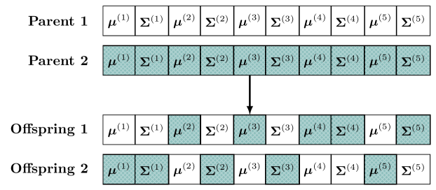
(a) Crossover

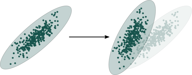
(b) Mutation

Figure 1: Illustrations of the HAWKS genetic operators. Uniform crossover (a) is used to independently swap the means and covariances between two individuals. In (b), a single cluster is mutated where both the location (mean) and shape (covariance) have been randomly perturbed (the original cluster is shown again faded to illustrate the relative differences).

As is typical in an EA, the variation operators in HAWKS provide a further opportunity to integrate domain knowledge and focus the search. Specifically, a close alignment between the generating model used (i.e. the representation of an individual cluster and partition) and the operators is crucial to optimization performance and the types of datasets that can be obtained. In the following, we describe the variation operators designed for the multivariate Gaussian distributions utilized as the generating model in our experiments.

III-E1 Crossover

For recombination between individuals, HAWKS uses a high-level uniform crossover scheme where the components defining each cluster distribution (in our Gaussian case, $\bm{\mu}$ and $\bm{\Sigma}$) can be swapped separately, as illustrated in Fig. 1a.

III-E2 Mutation

Meaningful mutations of a cluster require careful design of a geometrically relevant operator that is relevant for the distribution being used. In our Gaussian case, we use a separate operator for the mean and covariance terms.

A key issue identified in [47] was the drift of the mean operator in higher dimensions. The original operator shifts the mean to a random nearby point; at higher dimensionality there are an increasing number of directions that point away from other clusters, and a random walk is thereby likely to increase the silhouette width at most steps. In the supplementary material (Section supp-sec:mutating), we test multiple new mutation operators (drawing inspiration from operators used in particle swarm optimization and differential evolution) to address this issue by directly considering the location of other clusters.

The resulting operator selected and used throughout this paper utilizes concepts from particle swarm optimization [57], where a combination of other centroids and a global representative is used to embed direction either towards or away from existing clusters, directly affecting the fitness. The new mean, $\bm{\mu}^{\prime(i)}$, is obtained as follows:

$$\small\bm{\mu}^{\prime(i)}=\begin{cases}\bm{\mu}^{(i)}+[w_{1}(\bm{\mu}^{(n)}-\bm{\mu}^{(i)})+w_{2}(\bar{\bm{\mu}}-\bm{\mu}^{(i)})]&\text{if }p\leq 0.5\\[5.69046pt] \bm{\mu}^{(i)}-[w_{1}(\bm{\mu}^{(n)}-\bm{\mu}^{(i)})+w_{2}(\bar{\bm{\mu}}-\bm{\mu}^{(i)})]&\text{if }p>0.5,\\ \end{cases}$$ (7)

where $\bm{\mu}^{(i)}$ is the current cluster mean, $\bm{\mu}^{(n)}$ is the mean of another randomly selected cluster, $\bar{\bm{\mu}}$ is the global mean across all data points, $w_{1}$ and $w_{2}$ are random weighting coefficients in the range $[0,1]$, and $p$ is a random coin-flip to decide whether to move away from or towards this weighted combination of an existing cluster mean and the global mean.

The covariance governs the shape of the cluster, affecting both the overlap between clusters and the capabilities of compactness-based algorithms (such as K-Means). To mutate the covariance, we rotate the cluster and scale its eigenvalues, effectively changing the shape of the cluster. Similar to the initialization, the rotation matrix is drawn from the Haar distribution [48], though here it is raised to a fractional power to avoid complete reorientation of the cluster. The scaling matrix, $S$, is drawn from a Dirichlet distribution in order to ensure that the resulting determinant is unchanged i.e. $\det(\widetilde{\bm{\Sigma}})=\det(S\cdot\widetilde{\bm{\Sigma}})$. Using an analogy, this has the same effect as rotating a balloon and applying pressure to the principal semi-axes, thereby changing the shape while maintaining the volume. The combined effect of both mutation operators is illustrated in Fig. 1b.

III-F Selecting a dataset

As previously discussed, we use stochastic ranking [54] to balance the satisfaction of the objective and constraint(s), which may be complementary or impossible to both fully satisfy. In brief, stochastic ranking using a bubble-sort-like procedure to rank the population, where individuals are compared on their fitness with probability $P_{f}$, and are otherwise compared on their constraint violation. By adjusting $P_{f}$, we can effectively weigh the satisfaction of the objective or the constraints, providing another way of controlling the properties of the resulting datasets. For example, if using only the overlap constraint in Index mode, setting $P_{f}$ to a higher value will add selection pressure to datasets with a silhouette width closer to $s_{t}$, potentially at the cost of a higher degree of overlap. Thus, unlike the traditional use of stochastic ranking that uses a narrow range of values for $P_{f}$ [58, 54] to avoid too much weighting towards the infeasible or feasible regions, we can use the entire range (as datasets that heavily violate the constraints may still be useful).

Similar to the original work [54], for environmental selection we use stochastic ranking to select the top $|\mathcal{P}|$ individuals from the sorted pool of parents and offspring. For parental selection, we use standard binary tournament where the rank is used to determine the winner (in lieu of using only the fitness) to ensure a continued selection pressure towards individuals that best satisfy the fitness and constraints as weighted by $P_{f}$.

IV Experimental Setup

In order to assess the capabilities of HAWKS, we have three primary aims in our experiments: (i) compare the diversity of performance of multiple, distinct clustering algorithms on datasets from HAWKS against that of other popular generators or dataset collections; (ii) compare the diversity across a distinct set of problem features, to see if datasets from HAWKS cover a wider space of properties than other datasets; and, (iii) gain insights into the algorithms themselves, utilizing the Versus mode of HAWKS to directly challenge clustering algorithms.

The remainder of this section describes our proposed problem features (Section IV-A), the generators and dataset collections we compare against (Section IV-B), and the relevant parameters HAWKS used in each experiment (Section IV-C).

IV-A Problem features

In order to measure dataset diversity (with respect to their inherent properties), we need to define a set of problem features describing properties relevant to algorithm performance. This is central to the algorithm selection problem (ASP), as these features are used to predict which algorithm is best for a given problem instance. These problem features are also vital for the creation of an instance space that visualizes the datasets, allowing identification of areas in the space where particular algorithms are most suitable.

In previously discussed work on the ASP for clustering, the problem features (also referred to as “meta-features”) used are statistical or information-theoretic, and not specific to clustering [38, 39]. The problem features previously used in [47] were also too simplistic, and coincided with parameters available in HAWKS, reducing the utility of the instance space.

As there are many properties that influence performance for a given clustering algorithm, and for most algorithms this aspect is not fully understood, a full complementary set of problem features is arguably impossible [12, 8, 36]. Nonetheless, going beyond simple statistical measures of the data by incorporating measures specific to clustering (especially those that make use of the generating model) should improve the discriminative power of the problem features. The remainder of this section describes our proposed set of problem features for this task.

To this end, we use the following problem features: average cluster eccentricity, connectivity, dimensionality, entropy of cluster sizes, number of clusters, average silhouette width, and the standard deviation of the silhouette width. For a full explanation of these problem features (both their formulation and the motivation behind their use), see Section supp-ssec:problem_features.

IV-B Other generators and datasets

To provide context for the diversity in performance and problem features for the datasets produced by HAWKS, we compare against multiple generators or collections of popular datasets that have been previously used to evaluate clustering algorithms. We briefly describe these below, though more details about the parameters used for these datasets, and how they compare (in terms of their size, dimensionality etc.) can be found in the supplementary material (Table S-supp-tab:dataset_params) and their respective papers.

IV-B1 HK

This is a collection of 350 datasets generated using the “ellipsoidal” generator proposed in [14], and used as a benchmark in [59]. For 35 unique combinations of the number of clusters and dimensionality, 10 datasets are generated.

IV-B2 QJ

We use the set of 243 datasets generated using the parameters proposed by Qiu and Joe [45]. The authors calculated three target separation values using their measure of separation: “close structure”, “separated”, and “well-separated”. Further complexity to these datasets is added by specifying varying proportions of noisy variables, alongside small variation in the number of dimensions.

IV-B3 SIPU

Fränti and Sieranoja [43] introduced a benchmark consisting of multiple sets of clustering datasets, of which we use the ‘S-sets’, ‘A-sets’, and ‘G2 sets’. These sets were originally intended to stress-test compactness-based algorithms, of which K-Means exhibited a wide range of performance. The ‘S-sets’ are all 2D data where $N=5000$ and $K=15$, but have different degrees of overlap between the clusters (determined by the aforementioned method of the closest centroid). The ‘A-sets’ are also 2D data with varying numbers of (equally-sized) clusters. The ‘G2 sets’ of datasets consist of two Gaussians with varying degrees of overlap, constant size ($N=2048$) and varying dimensionality (chosen across the range $2^{1},2^{2},\ldots,2^{10}$). The variance of overlap and high number of dimensions in this benchmark presents a variety of challenges for clustering algorithms.

IV-B4 UCI

The UCI Machine Learning Repository [42] is a popular source of datasets used for machine learning. As noted in [11, 43] the class labels do not necessarily translate to meaningful cluster labels, and thus these datasets may not be the most suitable for clustering. Nonetheless, they have seen extensive use in the clustering literature, and we include them for completeness. Specifically, we use the subset of 20 datasets used by Arbelaitz et al. [12].

IV-B5 UKC

These 8 real-world datasets, curated in [59], are the (anonymized) locations of different crimes. Alongside the UCI datasets, these will help provide insight into whether there are significant differences between the real-world and synthetic data (in terms of their problem features or clustering algorithm performance).

IV-C HAWKS configurations

In this section we highlight the key parameters for HAWKS, separating those that are common across all experiments and those adjusted for different modes. In particular, while the core EA parameters (population size, mutation probability etc.) remain the same across modes, in our experiment for the Index mode we vary the objective function target and constraint parameters to generate different datasets. In contrast, the constraint parameters remain fixed for the Versus mode experiment as the variation comes from selecting different pairs of clustering algorithms. The full configurations for both sets of experiments can be found on GitHub.

IV-C1 Common parameters

In both Index and Versus mode experiments, the following core EA parameters are used: $G_{\text{max}}=100$ generations, $\mathcal{P}=10$ individuals, $p_{c}=0.7$ crossover probability, and $p_{m}=1/K$ mutation probability for the mean and covariance mutation operators. The low population size was previously found to be sufficient for both diversity and convergence [47]. A sensitivity analysis for increasing both the number of generations and population size can be found in Section supp-ssec:sensitivity.

IV-C2 Solution selection

At the end of a run, a single dataset needs to be selected. Here, we simply select the individual with the highest fitness. Different choices are possible, e.g., due to our use of stochastic ranking, the individual with the highest (sorted) rank could be selected instead (though this had little effect on the experiments in this paper).

IV-C3 Analyzing benchmark dataset diversity (Index mode)

To test the ability of HAWKS to produce a variety of datasets, we vary several parameters to encourage coverage of our feature space:

• A poor and a high silhouette width ($s_{t}\in\{0.45,0.9\}$).

• Two upper thresholds for the $\mathit{overlap}$ constraint ($\mathit{overlap}\leq\{0,0.1\}$) to penalize any overlap, or penalize if more than 10% of the data points overlap.

• Two lower thresholds for the eccentricity constraint ($\lambda^{\mathit{ratio}}\geq\{1,50\}$) to allow for any amount of eccentricity, or encourage all clusters have some eccentricity.

• Two levels of dimensionality ($D\in\{2,50\}$), dataset size ($N\in\{500,2500\}$), and number of clusters ($K\in\{5,30\}$).

Of note is the use of $P_{f}=0.5$, which weights the fitness and constraints equally. By varying $s_{t}$, we directly attempt to generate datasets that either have poor cluster separation or are well-separated. Different values of the overlap and eccentricity constraints help further modulate the level of separation and the minimum cluster eccentricity. HAWKS is run 7 times for each of the 64 unique combinations of parameters listed above, resulting in 448 datasets.

As we aim to measure diversity in clustering performance, we need an objective way to measure this. We therefore use the ARI (see Section III-C2) to compare the ground truth (which we know for all datasets used here) with the assignments from each algorithm. For the clustering algorithms themselves, we select four well-established algorithms with distinct properties and inductive biases, allowing us to assess the diversity of challenges that the datasets pose. These are:

• Average-linkage — A hierarchical clustering method that uses the average distance between all points in a cluster when deciding which are the closest (and thus should be merged).

• Gaussian mixture models (GMM) — Probabilistic models which try to represent subpopulations (of the data) through a number of Gaussian distributions. To obtain a crisp clustering, each point is assigned to the cluster with the highest probability.

• K-Means++ — Proposed by Arthur and Vassilvitskii [60] to improve K-Means, the initialization scheme probabilistically selects cluster centres such that points that are further away from existing cluster centres are more likely to be selected.

• Single-linkage — In contrast to average-linkage, single-linkage considers the distance between two clusters as the shortest distance from any member of one cluster to any member of another.

Scikit-learn [61] was used for all clustering algorithms, using Euclidean distance and default parameters. To assess the maximum potential of each algorithm, we provide the true number of clusters for each dataset. Owing to the propensity of the linkage algorithms (particularly single-linkage) to be side-tracked by singleton clusters, we also run average- and single-linkage with double the true number of clusters [62].

IV-C4 Challenging specific algorithms (Versus mode)

To ascertain the capabilities of HAWKS’ Versus mode, we run each of the four clustering algorithms against the others in a head-to-head, with either as the ‘winner’ and ‘loser’, respectively.

Some pairings of algorithms (e.g. K-Means++ vs. GMM) are likely to be more competitive, due to shared capabilities and inductive biases. We expect this to translate into a reduction of the performance differences that can be observed (and thus a weaker fitness gradient). While the constraints are still important in such a scenario, we wish to avoid situations where the optimization is being mainly driven by reducing the constraint penalty. Rather than removing the constraints, we increase $P_{f}$ to emphasize a difference in algorithmic performance. This provides a useful lever for weighting the maximization of the performance difference against producing datasets that do not sacrifice cluster structure (e.g. through a high overlap). As such, we use $P_{f}=0.75$ in all head-to-head runs. Further adjustment of this parameter is encouraged for complex algorithm pairings.

Finally, all experiments presented for the Versus mode are run using $K=5$ clusters and $N=2000$ data points. The dimensionality is consistently set to $D=2$, ensuring a straightforward visualization of the datasets and enabling us to observe the properties of these datasets without concerns about information loss through projection.

V Experimental Results

In this section, we explore HAWKS’ ability to produce datasets that exhibit a broad range of properties and pose challenges to different clustering algorithms. Separate results for the Index and Versus modes highlight the general flexibility of our framework.

V-A Analyzing benchmark dataset diversity (Index mode)

This section presents the instance space constructed from our set of 7 problem features applied to the 1,176 datasets from 6 popular collections/generators and our generator HAWKS. We assess diversity by considering (i) the variation observed across problem features and (ii) the variation observed in the performance of 4 clustering algorithms.

First, we use the instance space to understand how the datasets are spread across the space, and if there are distinct patterns either in the sources of the datasets or in the performance of the clustering algorithms. The two principal components of the instance space shown in Fig. 2 account for $57.56\%$ of the variance, and so there is some information loss in the projection. Nevertheless, it is evident that the components capture a sufficient proportion of the variance to highlight some key differences between datasets.

The instance space in Fig. 2a uses colour and marker coding to flag up which collection each dataset comes from. Visualizations of how each problem feature varies across the space can be found in Fig. S-supp-fig:benchmark_features. The distinct spread of HAWKS datasets across the central part of the space is encouraging and highlights an appropriate level of diversity in terms of the problem features. Furthermore, the interpretation of the principal components (in terms of the underlying problem features), provides clear guidance on additional experiments that could be conducted to expand coverage in various directions. In contrast, the QJ datasets expand across a narrow band, indicating a lack of variance across the problem features. The SIPU datasets show a strong banding of instances, indicating that there is little variance among the datasets from each configuration (the separated datasets at the bottom of the space are the ‘G2 sets’, which have a much higher dimensionality than other datasets). The UCI datasets are spread across the upper-half of the space, though this is unfortunately due to a lack of structure (which we later explore when looking at clustering algorithm performance), as their higher connectivity indicates that the labels do not line up with a spatial perspective of clustering (shown in Fig. S-supp-fig:benchmark_connectivity). The UKC datasets do not seem to represent anything extraordinary with regards to the problem features we use here, leading to the conclusion that either the synthetic datasets used here are not too dissimilar to real-world data or our set of problem features does not capture some aspect of complexity that they uniquely exhibit. Notably, the HK datasets are distinct from every other collection, indicating that they have unique characteristics. As shown in Fig. S-supp-fig:benchmark_eccen, the main difference is the average eccentricity of the clusters, which is higher than in any other collection. As these datasets originate from the “ellipsoidal” generator, which was designed exclusively to create eccentric clusters in higher dimensions, this is unsurprising. Of interest, however, is whether this leads to a distinct difference in the relative performance of clustering algorithms on that benchmark suite.

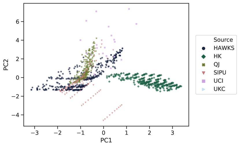
(a) Dataset source

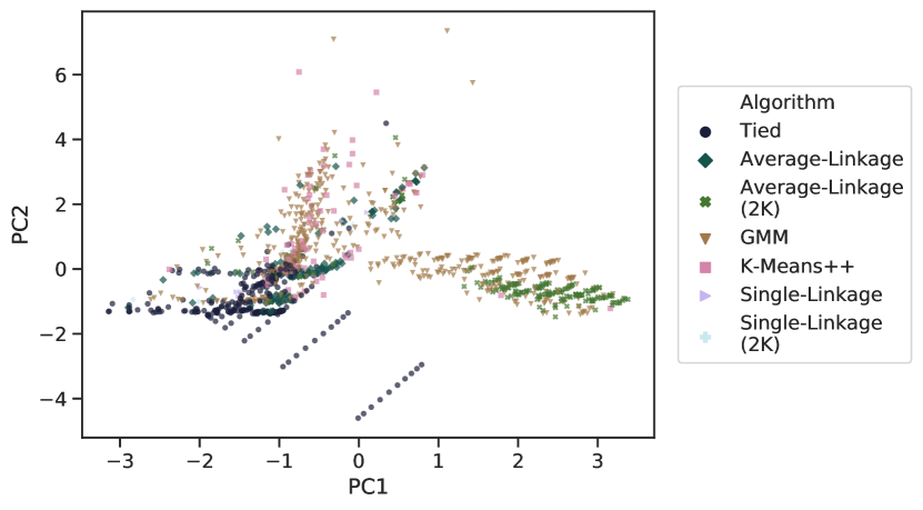
(b) Algorithm with highest ARI

Figure 2: Two instance spaces, with the source of the dataset (a) or clustering algorithm with the highest ARI (b) highlighted. The 7 problem features are projected down to 2D using PCA. The contribution of each problem feature to the two principal components is $\begin{bmatrix}-0.029&0.208&0.519&0.308&0.506&-0.256&0.520\\ 0.675&-0.355&-0.206&-0.007&-0.120&-0.555&0.231\end{bmatrix}$ for the connectivity, dimensionality, average eccentricity, entropy, number of clusters, silhouette width (average), and silhouette width (standard deviation) respectively.

To consider this aspect, Fig. 2b shows the instance space again with the clustering algorithm achieving the highest ARI for a given dataset highlighted. The ‘tied’ category is used when at least two algorithms were able to achieve the same ARI, which in every case was 1 and thus the dataset was trivial to cluster. This visualization permits identification of potential footprints, though the full information is tabulated in Table I for completeness. It is evident that there are some areas of the space that correlate with a high performance of a particular algorithm, and this happens for the HK benchmark suite in particular where the highly ellipsoidal clusters consistently favour GMM or average-link with the higher setting of $K$.

In the more central part of the instance space, however, such footprints are unclear, indicating a complex performance landscape. This could be a consequence of the projection (which may lose too much information to fully distinguish the datasets), or may point to the role of other features that have not yet been captured here, but distinctly impact on performance. Notably, variation in the identity of the best performing algorithm is the most pronounced for the HAWKS benchmark (see Table I), which is the only collection of datasets where every algorithm was best for a particular dataset. As this was achieved through just a few parameter settings, this is encouraging for the potential of HAWKS to generate diverse datasets.

TABLE I: Number of times (as a percentage of the total number of datasets for each source) each algorithm achieved the highest ARI for a given dataset. The best performing algorithm on each data source is highlighted in bold.

	Average-	Average-		K-	Single-	Single-
Source	Linkage	Linkage	GMM	Means	Linkage	Linkage	Tied
		($2K$)		++		($2K$)
HAWKS	0.261	0.056	0.239	0.056	0.016	0.011	0.362
HK [14]	–	0.426	0.569	0.006	–	–	–
QJ [45]	0.008	0.021	0.646	0.082	–	0.004	0.239
SIPU [43]	–	–	0.106	0.202	–	–	0.692
UCI [42]	0.100	0.150	0.500	0.200	–	–	0.050
UKC [59]	–	–	0.625	0.124	–	–	0.250

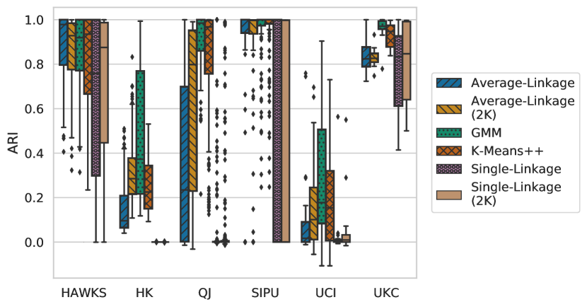
Figure 3: Clustering performance for each algorithm for each set of datasets.

To further examine the performance variation of the clustering algorithms across these datasets, Fig. 3 shows boxplots for the aggregated performance of each algorithm for each group of datasets. Here, larger boxplots indicate a greater variety of performance for that clustering algorithm, which is preferred. For HAWKS, the boxplots indicate that its datasets elicit a broad range of performance across all algorithms, though the high median ARIs for all algorithms indicate that in general the datasets were not that difficult. As we discourage overlap and half of the datasets were optimized to have a high silhouette width ($s_{t}=0.9$), this is somewhat expected and could be addressed by revised parameter choices.

The near-perfect average performance for all algorithms but single-linkage on the SIPU datasets indicate their relative simplicity. Similarly, the poor average performance across the UCI datasets is consistent with the low connectivity and silhouette width values previously observed in the instance space, and points to weakly defined structure of the ground truth. The HK datasets show a reasonable diversity of performance, and the significantly lower mean ARI indicates that these are much harder datasets. This may be in part due to the much higher eccentricity of these clusters, but also potentially due to a greater variance in the silhouette width (Fig. S-supp-fig:benchmark_sw-std), indicating that many data points on the edges of clusters are closer to the points in other clusters than to points in their own. The high performance of all algorithms on the UKC datasets indicates that the clusters in this real-world dataset are generally well-defined. This is consistent with the instance space which provided no evidence of unusual complexity.

To include considerations of significance into our analysis, we follow the approach outlined by Demšar [63] to compare multiple methods across multiple datasets. In brief, a Friedman test is used to rank each competing algorithm for each dataset, where the null hypothesis is that all algorithms have equal ranks. As rejection indicates at least one algorithm is significantly different, the (two-tailed) Nemenyi test [64] is used as a post-hoc test to ascertain which algorithm is different by calculating the critical difference (CD), which is the minimum that two average ranks must differ by to be significantly ($p<0.05$) different. We illustrate the results using CD diagrams, which show the average rank of each algorithm across all datasets, with solid lines connecting algorithms whose difference in rank is less than the CD. Well-ordered rankings of algorithms indicate a lack of variance in performance (as an algorithm is consistently bad or good), whereas if all algorithms had an average rank of 3.5 (and thus clustered in the middle of the CD diagram), this would show that the datasets have an equal spread of difficulty for these clustering algorithms.

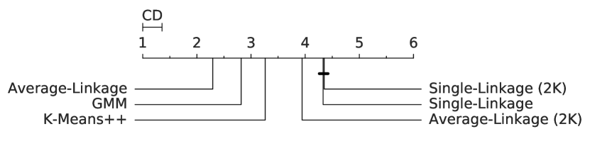
(a) HAWKS

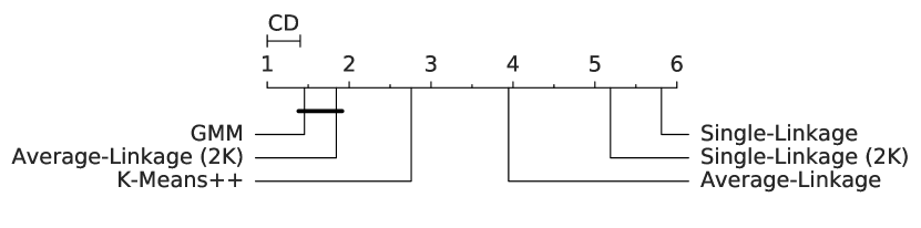
(b) HK

Figure 4: Critical difference (CD) diagrams, showing the mean rank (in terms of ARI) for the HAWKS and HK datasets, for each algorithm. Algorithms connected by solid lines are not significantly different according to a two-tailed Nemenyi test. CD diagrams for the other dataset sources can be found in Fig. S-supp-fig:cd_extras.

We show the CD diagrams for the HAWKS and HK generators in Fig. 4 (as these two generators showed the greatest diversity in the boxplots). As evident from the CD diagram, the ranks of the algorithms are more similar for HAWKS, whereas there is a clearer superiority for a subset of algorithms with the HK datasets. The best-performing algorithm for HAWKS was average-linkage, which highlights the variety of cluster structures that can be generated (as the representation uses purely Gaussian clusters, one might have expected that GMM would on average perform the best). The eccentricity of the generated clusters is reflected in the higher average rank of GMM over K-Means++. Furthermore, the poor performance of single-linkage (using both $K$ and $2K$) indicates that there is (on average) insufficient cluster separation to avoid the ‘chaining’ effect [62], where there is at least one pair of points in different clusters that are closer than a pair of points within a cluster, thereby forming a ‘bridge’ between clusters.

As shown in Table I, all of the generators struggle to produce datasets that single-linkage is uniquely better at, suggesting a possible lower utility of this algorithm, in general. To further investigate this, and to create a fully comprehensive benchmark, it would be of interest to more directly generate datasets that favour single-linkage. In contrast to existing generators, the Versus mode in HAWKS facilitates this direct generation, and the results from this mode are discussed in the next section.

V-B Generating datasets that challenge specific algorithms (Versus mode)

In this section, we present the results of running HAWKS in Versus mode, such that we evolve datasets to directly maximize the performance difference between pairs of algorithms. As seen in Section V-A, most current generators have some bias towards a particular algorithm, and no generator (except HAWKS, though not consistently so) was able to produce datasets that were uniquely suited to single-linkage.

First, we need to look at the broad capability of the Versus mode in producing a performance differential in the various head-to-heads. In Fig. 5, we can see a grid of plots showing the performance (ARI) of every algorithm against every other. Each line (in the off-diagonal plots) represents the best dataset from a single run, showing the ARI for ‘winning’ (left) and ‘losing’ (right) algorithms. Here, the angle of the lines indicate the magnitude of the performance difference, and the spread shows the consistency of HAWKS across runs. The plots on the diagonal aggregate the performance for that particular algorithm, e.g. the bottom-right plot indicates that HAWKS was able to produce datasets that single-linkage performed both very well and very poorly on, dependent on whether it was designated as the winner or loser of the head-to-head.

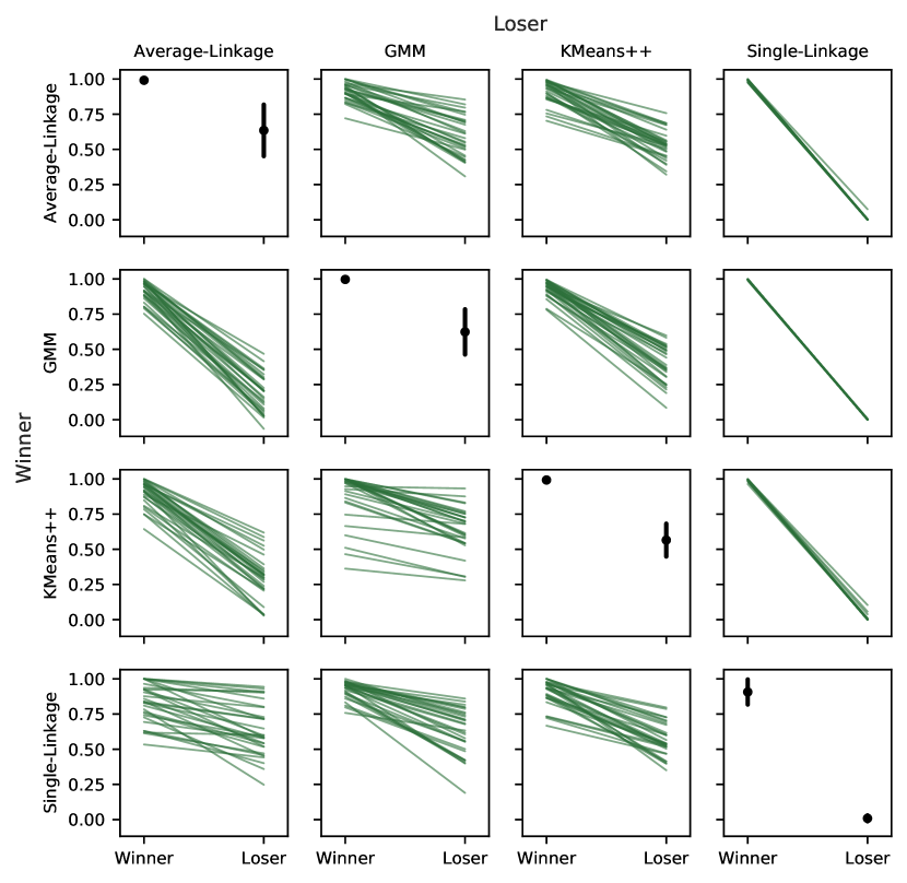
Figure 5: Performance (ARI) for each algorithm as the winner (row) and loser (column). Each line represents the best individual from a single run, connecting the ARI obtained for $\mathcal{A}_{w}$ and $\mathcal{A}_{l}$. On the diagonal, the average (and standard deviation) performance is aggregated for that individual as the winner and loser, indicating the overall capability of HAWKS to produce datasets that are simple and difficult for that algorithm.

There are some clear differences between certain pairings of algorithms. As hinted in Section V-A, HAWKS is consistently able to generate maximal (i.e. $\phi(\mathcal{A}_{w})-\phi(\mathcal{A}_{l})\approx 1$) performance difference when single-linkage is $\mathcal{A}_{l}$, but the performance difference appears minimal for single-linkage vs. average-linkage, indicating that any weaknesses specific to average-link are not weaknesses that single-link can exploit. The average ARI for average-linkage, GMM and K-Means++ when set as the ‘loser’ ($\mathcal{A}_{l}$) indicates a difficulty in consistently generating datasets that these algorithms perform very poorly on. This is not unexpected, given the generating model used. As long as clusters are not fully overlapping (which we discourage with our $\mathit{overlap}$ constraint) we expect these algorithms to identify some elements of the clusters, making an ARI close to 0 unlikely.

To evaluate the influence of algorithm initialization, the stochastic algorithms (GMM and K-Means++) are re-run with a different initialization (Fig. S-supp-fig:versus_grid_2). While K-Means++ was largely unchanged, there was an average ARI increase (as $\mathcal{A}_{l}$) of 0.13 for GMM, highlighting that in some cases the lower performance was due to a poor initialization. The average ARI did, however, slightly decrease (as $\mathcal{A}_{w}$), highlighting the potential disadvantage of these stochastic algorithms over linkage-based algorithms as they converge to local minima. This suggests another use case for HAWKS. When given an infinite budget of initializations and picking the best, we expect these algorithms to perform better. The robustness of the initialization method can be assessed, however, by investigating how often the algorithm is still able to achieve good performance with a limited budget.

In order to investigate the ability of the Versus mode to grant algorithmic insight, we need to inspect the structures HAWKS discovered for different algorithm combinations. For this, it is important to identify where HAWKS struggles to generate datasets that favour one algorithm over another. We can then try to establish whether this is due to the superiority of one algorithm over another, or the inability of HAWKS to generate structures with properties that would differentiate them. For brevity, the following sections discuss some interesting examples for a subset of the scenarios (shown in Fig. 6). Further examples of the algorithm pairings can be found in the supplementary material (Section supp-sec:versus).

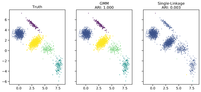
(a) GMM vs. single-linkage

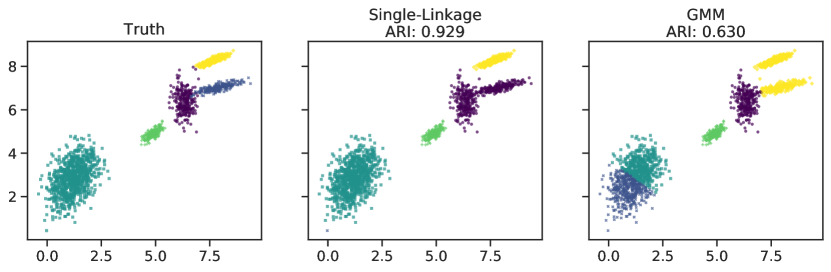
(b) Single-linkage vs. GMM

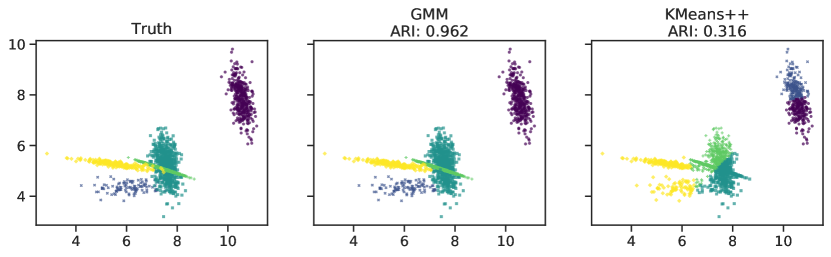
(c) GMM vs. K-Means++

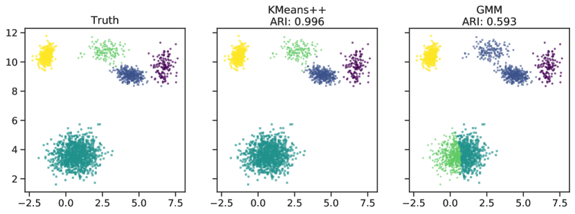
(d) K-Means++ vs. GMM

Figure 6: Examples of datasets for the listed head-to-heads. Each figure shows the ground truth (left column), and the cluster assignment for each algorithm with the associated ARI (middle and right columns).

V-B1 GMM vs. single-linkage

Owing to the Gaussian representation that HAWKS uses, and the known issues of single-linkage, this scenario is expected to provide a large performance difference. Fig. 6a shows that HAWKS achieves this performance difference by exploiting the aforementioned ‘chaining’ effect of single-linkage [62]. Discovering this requires iterative movement of the clusters in order for the data points to be close enough to induce this effect, supporting the utility of our mutation operators’ nuanced ability to adjust the location of clusters.

V-B2 Single-linkage vs. GMM

The reverse scenario should be much harder for HAWKS, as GMM is largely insensitive to eccentricity and naturally fits our cluster representation. As exemplified in Fig. 6b (and observed in the other datasets produced), HAWKS tends to place large clusters far away from several smaller compact clusters in order to increase the chance of a poor initialization from GMM, exploiting the stochasticity of this method.

V-B3 GMM vs. K-Means++

In Fig. 6c we can see that a key exploit, as discovered by HAWKS, is the inability of K-Means++ to handle eccentric clusters. The example highlights significant differences between the use of mixture models and an algorithm relying on assignment to the closest centroid. A clear performance differential is found on this dataset, despite basic similarities in the inductive biases of the two algorithms.

V-B4 K-Means++ vs. GMM

As both algorithms are well-suited for compact clusters, eccentricity is not a characteristic that can be used for differentiating performance in this scenario. Here, HAWKS exploits GMM’s previously-mentioned weakness (of sub-dividing a single large cluster) during its initialization stage. K-Means++ is less sensitive to this problem due to its improved initialization routine. This shows the utility of HAWKS in identifying relative strengths and weaknesses of specific algorithms, which could aid in algorithmic development (e.g. when empirically comparing initialization schemes).

The datasets in the Versus mode are optimized towards a performance differential between the algorithms, rather than towards a cluster structure specified by the cluster validity index (as done in the Index mode). It is therefore of interest to investigate how these datasets compare in terms of problem feature diversity. For this, we add the 30 datasets from each of the 12 head-to-heads to the instance space created in Section V-A (using the same principal components).

In Fig. 7, we have highlighted the datasets from the Index and Versus modes (with the other datasets in grey for reference). Clearly, we are able to generate datasets that are notably different in terms of their problem features (and thus properties). In particular, there are many datasets in the region where previously only HK produced datasets, further highlighting the flexibility of our generating mechanism in covering additional regions, as objective function, clustering algorithms, and other parameters are varied. The problem feature values are tabulated for all dataset sources, including those from Index and Versus modes, in Table S-supp-tab:problem_features.

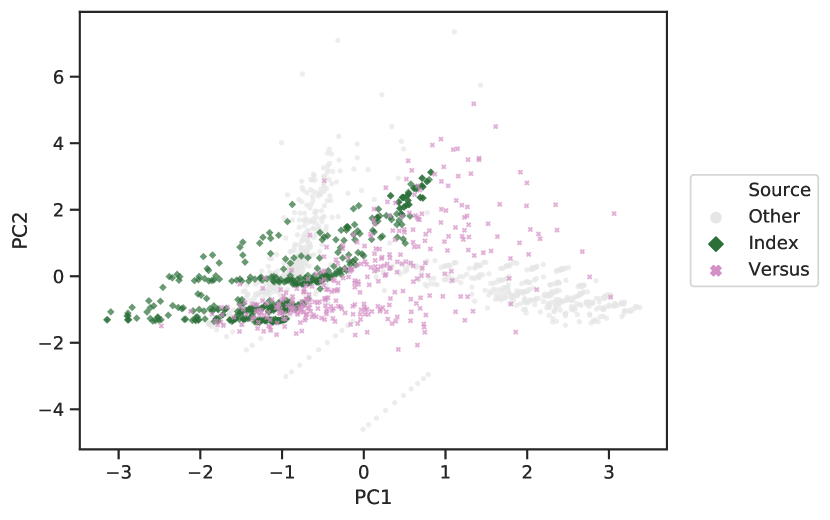
Figure 7: Instance space created in Section V-A with the datasets produced by the two modes of HAWKS highlighted (the ‘Other’ points are the other datasets).

VI Conclusion

Clustering is a vital tool for pattern discovery, but it is often unclear which clustering algorithm is the most appropriate for a given dataset. An optimal choice requires an accurate understanding of the data properties as well as the strengths and weaknesses of candidate algorithms. Both types of information are difficult to come by in typical real-world settings.

Synthetic benchmark datasets play an important role in improving our understanding of the former, i.e. to examine the specific strengths and capabilities of a given clustering method. Their specific advantage is the availability of a known generating model, which allows researchers to relate aspects of the true cluster structure to algorithm performance. Unfortunately, available synthetic benchmarks for cluster analysis cover a limited variety of structural aspects, and there are no existing generators that have been designed with a wider flexibility in mind.

Our framework HAWKS employs the power of an EA to better meet the challenges highlighted above, and to generate more diverse collections of benchmarks, in particular. When compared to existing clustering benchmarks, HAWKS is found to generate datasets exhibiting more feature diversity and eliciting more variation in algorithm performance. The modular nature of HAWKS provides much opportunity for extension; additional distributions can be added to increase dataset diversity, and extension to temporal/streaming data would greatly benefit a currently underserved application. Further work to improve the ability of the instance space to distinguish algorithmic footprints, by further enriching the set of problem features and improving the projection methodology, is also needed.

Finally, HAWKS can be modified to directly generate datasets that are either simple or difficult for a given algorithm, facilitating a deeper understanding of existing algorithms and potentially informing algorithm development. This provides a new avenue for “controlled experimentation” with clustering algorithms, which does not rely on the use of over-simplified toy datasets. Investigations into the use of this Versus mode in conjunction with more complex clustering algorithms, could further test HAWKS’ capabilities and may provide novel insights into the inductive biases and performance of these algorithms.

Cameron Shand (memberreceived the M.Eng. degree in biochemical engineering from UCL (London, UK) in 2015, and the Ph.D. degree in computer science from the University of Manchester (Manchester, UK) in 2020. Since 2020, he is currently a Research Fellow in Disease Progression Modelling and Machine Learning for Clinical Trials with the Centre for Medical Image Computing at UCL. His research interests include the development of unsupervised machine learning techniques and their clinical application, and the role of synthetic data in understanding and improving clustering methods.

Richard Allmendinger (Member, IEEE) received a Diplom in business engineering from Karlsruhe Institute of Technology, and the Ph.D. degree in computer science from the University of Manchester (UoM), UK. He is currently a Senior Lecturer (Associate Professor) in Decision Sciences at UoM and an Alan Turing Fellow, having worked previously as a postdoc at the biochemical engineering department, University College London. His research interests include multi-objective, dynamic, safe, and expensive optimization and machine learning. He is a Vice-Chair of the IEEE CIS Bioinformatics and Bioengineering (BB) Technical Committee, Co-Founder of the IEEE CIS Task Force on Optimization Methods in BB, and on the Editorial Board of several international journals.

Julia Handl received the B.Sc. (Hons.) degree in computer science from Monash University, Melbourne, VIC, Australia, in 2001, the M.Sc. degree in computer science from the University of Erlangen-Nuremberg, Erlangen, Germany, in 2003, and the Ph.D. degree in bioinformatics from the University of Manchester, Manchester, U.K., in 2006. From 2007 to 2011, she held an MRC Special Training Fellowship with the University of Manchester, and is currently an Alan Turing Fellow and Professor in the Management Sciences Group, Alliance Manchester Business School, Manchester. Her research interests include theoretical and empirical work related to the development and use of machine learning and optimization approaches in a variety of application areas.

Andrew Webb received the B.Sc. (Hons.) degree in computer science from the University of Manchester (Manchester, UK) in 2010, and the Ph.D. in computer science from the University of Manchester in 2016. From 2017 to 2019 he was a Research Associate at the University of Manchester, with research interests in deep learning and ensemble methods in machine learning. He is currently a Machine Learning Research and Development Engineer at vTime Limited, Liverpool, UK.

John Keane holds the MG Singh Chair of Data Engineering in the Department of Computer Science, School of Engineering, University of Manchester and is an Honorary Professor of Data Analytics at the Alliance Manchester Business School. He has previous commercial experience with Phillips, Fujitsu, and the TSB Bank. His research focuses on data analytics and decision science.

References

- [1] J. Handl, J. D. Knowles, and D. B. Kell, “Computational cluster validation in post-genomic data analysis,” Bioinformatics, vol. 21, no. 15, pp. 3201–3212, 2005.
- [2] U. Maulik, S. Bandyopadhyay, and A. Mukhopadhyay, Multiobjective Genetic Algorithms for Clustering - Applications in Data Mining and Bioinformatics. Springer, 2011.
- [3] R. Xu and D. C. Wunsch, “Clustering algorithms in biomedical research: A review,” IEEE Rev. Biomed. Eng., vol. 3, pp. 120–154, 2010.
- [4] M. Ahmed, A. N. Mahmood], and J. Hu, “A survey of network anomaly detection techniques,” Journal of Network and Computer Applications, vol. 60, pp. 19–31, 2016.
- [5] Z. Ma, J. M. R. Tavares, R. N. Jorge, and T. Mascarenhas, “A review of algorithms for medical image segmentation and their applications to the female pelvic cavity,” Computer Methods in Biomechanics and Biomedical Engineering, vol. 13, no. 2, pp. 235–246, 2010.
- [6] S. Dolnicar, “A review of data-driven market segmentation in tourism,” Journal of Travel & Tourism Marketing, vol. 12, no. 1, pp. 1–22, 2002.
- [7] M. S. Handcock, A. E. Raftery, and J. M. Tantrum, “Model-based clustering for social networks,” Journal of the Royal Statistical Society: Series A (Statistics in Society), vol. 170, no. 2, pp. 301–354, 2007.
- [8] C. Hennig, “What are the true clusters?” Pattern Recognition Letters, vol. 64, pp. 53–62, 2015.
- [9] A. K. Jain, M. N. Murty, and P. J. Flynn, “Data clustering: A review,” ACM Computing Surveys, vol. 31, no. 3, pp. 264–323, 1999.
- [10] G. W. Milligan, Clustering validation: results and implications for applied analyses. World Scientific Publishing Company, 1996, ch. 9, pp. 341–375.
- [11] U. von Luxburg, R. C. Williamson, and I. Guyon, “Clustering: Science or art?” in Unsupervised and Transfer Learning – Workshop held at ICML 2011, ser. JMLR Proc., vol. 27. JMLR.org, 2012, pp. 65–80.
- [12] O. Arbelaitz, I. Gurrutxaga, J. Muguerza, J. M. Pérez, and I. Perona, “An extensive comparative study of cluster validity indices,” Pattern Recognition, vol. 46, no. 1, pp. 243–256, 2013.
- [13] J. N. Hooker, “Testing heuristics: We have it all wrong,” Journal of Heuristics, vol. 1, no. 1, pp. 33–42, 1995.
- [14] J. Handl and J. D. Knowles, “Improvements to the scalability of multiobjective clustering,” in Proc. IEEE Congress on Evolutionary Computation, CEC 2005, 2-4 September 2005, Edinburgh, UK. IEEE, 2005, pp. 2372–2379.
- [15] K. Smith-Miles and T. T. Tan, “Measuring algorithm footprints in instance space,” in Proc. IEEE Congress on Evolutionary Computation, CEC 2012. IEEE, 2012, pp. 1–8.
- [16] N. Macià and E. Bernadó-Mansilla, “Towards uci+: a mindful repository design,” Information Sciences, vol. 261, pp. 237–262, 2014.
- [17] O. Mersmann, M. Preuss, and H. Trautmann, “Benchmarking evolutionary algorithms: Towards exploratory landscape analysis,” in International Conf. on Parallel Problem Solving from Nature 2010. Springer, 2010, pp. 73–82.
- [18] J. Schmidhuber, “Deep learning in neural networks: An overview,” Neural Networks, vol. 61, pp. 85–117, 2015.
- [19] D. H. Wolpert, “The lack of A priori distinctions between learning algorithms,” Neural Computation, vol. 8, no. 7, pp. 1341–1390, 1996.
- [20] J. R. Rice, “The algorithm selection problem,” Advances in Computers, vol. 15, pp. 65–118, 1976.
- [21] K. Smith-Miles, “Cross-disciplinary perspectives on meta-learning for algorithm selection,” ACM Computing Surveys, vol. 41, no. 1, pp. 6:1–6:25, 2008.
- [22] K. Smith-Miles, D. Baatar, B. Wreford, and R. Lewis, “Towards objective measures of algorithm performance across instance space,” Computers & Operations Research, vol. 45, pp. 12–24, 2014.
- [23] K. Smith-Miles and L. Lopes, “Measuring instance difficulty for combinatorial optimization problems,” Computers & Operations Research, vol. 39, no. 5, pp. 875–889, 2012.
- [24] K. Smith-Miles and S. Bowly, “Generating new test instances by evolving in instance space,” Computers & Operations Research, vol. 63, pp. 102–113, 2015.
- [25] M. A. Muñoz, L. Villanova, D. Baatar, and K. Smith-Miles, “Instance spaces for machine learning classification,” Machine Learning, vol. 107, no. 1, pp. 109–147, 2018.
- [26] M. Birattari, Tuning Metaheuristics - A Machine Learning Perspective, ser. Studies in Computational Intelligence. Springer, 2009, vol. 197.
- [27] F. Hutter, L. Kotthoff, and J. Vanschoren, Eds., Automated Machine Learning - Methods, Systems, Challenges, ser. The Springer Series on Challenges in Machine Learning. Springer, 2019.
- [28] M. López-Ibáñez, J. Dubois-Lacoste, L. P. Cáceres, M. Birattari, and T. Stützle, “The irace package: Iterated racing for automatic algorithm configuration,” Operations Research Perspectives, vol. 3, pp. 43–58, 2016.
- [29] P. Kerschke and M. Preuss, “Exploratory landscape analysis: advanced tutorial at GECCO 2017,” in Genetic and Evolutionary Computation Conf., 2017, Companion Material Proc., P. A. N. Bosman, Ed. ACM, 2017, pp. 762–781.
- [30] L. Kotthoff, P. Kerschke, H. H. Hoos, and H. Trautmann, “Improving the state of the art in inexact TSP solving using per-instance algorithm selection,” in Learning and Intelligent Optimization - 9th International Conf., LION 2015. Revised Selected Papers, ser. Lecture Notes in Computer Science, vol. 8994. Springer, 2015, pp. 202–217.
- [31] O. Mersmann, B. Bischl, H. Trautmann, M. Preuss, C. Weihs, and G. Rudolph, “Exploratory landscape analysis,” in Proc. Genetic and Evolutionary Computation Conf., GECCO 2011, N. Krasnogor and P. L. Lanzi, Eds. ACM, 2011, pp. 829–836.
- [32] G. C. Bowker and S. L. Star, Sorting Things Out: Classification and its Consequences. MIT Press, 2000.
- [33] B. S. Everitt, S. Landau, M. Leese, and D. Stahl, Cluster Analysis, 5th ed. Wiley Publishing, 2011.
- [34] S. Ben-David, “Clustering — what both theoreticians and practitioners are doing wrong,” in Proc. 32nd AAAI Conf. on Artificial Intelligence 2018. AAAI Press, 2018, pp. 7962–7964.
- [35] J. M. Kleinberg, “An impossibility theorem for clustering,” in Advances in Neural Information Processing Systems, 2003, pp. 463–470.
- [36] C. Hennig, “Some thoughts on simulation studies to compare clustering methods,” Archives of Data Science, Series A, vol. 5, no. 1, pp. P24, 21 S. online, 2018.
- [37] I. V. Mechelen, A.-L. Boulesteix, R. Dangl, N. Dean, I. Guyon, C. Hennig, F. Leisch, and D. Steinley, “Benchmarking in cluster analysis: A white paper,” 2018.
- [38] D. G. Ferrari and L. N. de Castro, “Clustering algorithm selection by meta-learning systems: A new distance-based problem characterization and ranking combination methods,” Information Sciences, vol. 301, pp. 181–194, 2015.
- [39] R. G. F. Soares, T. B. Ludermir, and F. de A. T. de Carvalho, “An analysis of meta-learning techniques for ranking clustering algorithms applied to artificial data,” in Artificial Neural Networks - ICANN 2009, ser. Lecture Notes in Computer Science, vol. 5768. Springer, 2009, pp. 131–140.
- [40] G. W. Milligan, “An examination of the effect of six types of error perturbation on fifteen clustering algorithms,” Psychometrika, vol. 45, no. 3, pp. 325–342, Sep 1980.
- [41] M. Z. Rodriguez, C. H. Comin, D. Casanova, O. M. Bruno, D. R. Amancio, L. d. F. Costa, and F. A. Rodrigues, “Clustering algorithms: A comparative approach,” PLOS ONE, vol. 14, no. 1, pp. 1–34, 01 2019.
- [42] D. Dheeru and E. Karra Taniskidou, “UCI machine learning repository,” 2017.
- [43] P. Fränti and S. Sieranoja, “K-means properties on six clustering benchmark datasets,” Applied Intelligence, vol. 48, no. 12, pp. 4743–4759, 2018.
- [44] J. Handl and J. Knowles, “Feature subset selection in unsupervised learning via multiobjective optimization,” International Journal of Computational Intelligence Research, vol. 2, no. 3, pp. 217–238, 2006.
- [45] W. Qiu and H. Joe, “Generation of random clusters with specified degree of separation,” Journal of Classification, vol. 23, no. 2, pp. 315–334, 2006.
- [46] ——, “Separation index and partial membership for clustering,” Computational Statistics & Data Analysis, vol. 50, no. 3, pp. 585–603, 2006.
- [47] C. Shand, R. Allmendinger, J. Handl, A. M. Webb, and J. Keane, “Evolving controllably difficult datasets for clustering,” in Proc. Genetic and Evolutionary Computation Conf., GECCO 2019. ACM, 2019, pp. 463–471.
- [48] G. W. Stewart, “The efficient generation of random orthogonal matrices with an application to condition estimators,” SIAM Journal on Numerical Analysis, vol. 17, no. 3, pp. 403–409, 1980.
- [49] R. Maitra and V. Melnykov, “Simulating data to study performance of finite mixture modeling and clustering algorithms,” Journal of Computational and Graphical Statistics, vol. 19, no. 2, pp. 354–376, 2010.
- [50] S. E. Akhanli and C. Hennig, “Comparing clusterings and numbers of clusters by aggregation of calibrated clustering validity indexes,” Statistics and Computing, vol. 30, no. 5, pp. 1523–1544, 2020.
- [51] P. J. Rousseeuw, “Silhouettes: a graphical aid to the interpretation and validation of cluster analysis,” Journal of Computational and Applied Mathematics, vol. 20, pp. 53–65, 1987.
- [52] J. Xie, R. Girshick, and A. Farhadi, “Unsupervised deep embedding for clustering analysis,” in Proc. 33rd Int. Conf. on Machine Learning - Volume 48, ser. ICML’16. JMLR.org, 2016, pp. 478––487.
- [53] L. Hubert and P. Arabie, “Comparing partitions,” Journal of Classification, vol. 2, no. 1, pp. 193–218, 1985.
- [54] T. P. Runarsson and X. Yao, “Stochastic ranking for constrained evolutionary optimization,” IEEE Trans. Evol. Comput., vol. 4, no. 3, pp. 284–294, 9 2000.
- [55] E. Nowakowska, J. Koronacki, and S. Lipovetsky, “Tractable measure of component overlap for gaussian mixture models,” 2014.
- [56] H. Sun and S. Wang, “Measuring the component overlapping in the gaussian mixture model,” Data Min. Knowl. Discov., vol. 23, no. 3, pp. 479–502, 2011. [Online]. Available: https://doi.org/10.1007/s10618-011-0212-3
- [57] J. Kennedy and R. Eberhart, “Particle swarm optimization,” in Proc. of International Conf. on Neural Networks (ICNN’95). IEEE, 1995, pp. 1942–1948.
- [58] B. Li, K. Tang, J. Li, and X. Yao, “Stochastic ranking algorithm for many-objective optimization based on multiple indicators,” IEEE Trans. Evol. Comput., vol. 20, no. 6, pp. 924–938, 2016.
- [59] M. Garza-Fabre, J. Handl, and J. D. Knowles, “An Improved and More Scalable Evolutionary Approach to Multiobjective Clustering,” IEEE Trans. Evol. Comput., vol. 22, no. 4, pp. 515–535, 2017.
- [60] D. Arthur and S. Vassilvitskii, “k-means++: The advantages of careful seeding,” in Proc. 18th Annual ACM-SIAM Symp. on Discrete Algorithms, SODA. SIAM, 2007, pp. 1027–1035.
- [61] F. Pedregosa, G. Varoquaux, A. Gramfort, V. Michel, B. Thirion, O. Grisel, M. Blondel, P. Prettenhofer, R. Weiss, V. Dubourg, J. Vanderplas, A. Passos, D. Cournapeau, M. Brucher, M. Perrot, and E. Duchesnay, “Scikit-learn: Machine learning in Python,” Journal of Machine Learning Research, vol. 12, pp. 2825–2830, 2011.
- [62] L. Hubert, “Approximate evaluation techniques for the single-link and complete-link hierarchical clustering procedures,” Journal of the American Statistical Association, vol. 69, no. 347, pp. 698–704, 1974.
- [63] J. Demšar, “Statistical comparisons of classifiers over multiple data sets,” Journal of Machine Learning Research, vol. 7, no. Jan, pp. 1–30, 2006.
- [64] P. Nemenyi, “Distribution-free multiple comparisons,” Ph.D. dissertation, Princeton University, 1963.