Traveling Repairperson, Unrelated Machines, and Other Stories About Average Completion Times

Abstract

We present a unified framework for minimizing average completion time for many seemingly disparate online scheduling problems, such as the traveling repairperson problems (TRP), dial-a-ride problems (DARP), and scheduling on unrelated machines.

We construct a simple algorithm that handles all these scheduling problems, by computing and later executing auxiliary schedules, each optimizing a certain function on already seen prefix of the input. The optimized function resembles a prize-collecting variant of the original scheduling problem. By a careful analysis of the interplay between these auxiliary schedules, and later employing the resulting inequalities in a factor-revealing linear program, we obtain improved bounds on the competitive ratio for all these scheduling problems.

In particular, our techniques yield a $4$-competitive deterministic algorithm for all previously studied variants of online TRP and DARP, and a $3$-competitive one for the scheduling on unrelated machines (also with precedence constraints). This improves over currently best ratios for these problems that are $5.14$ and $4$, respectively. We also show how to use randomization to further reduce the competitive ratios to $1+2/\ln 3<2.821$ and $1+1/\ln 2<2.443$, respectively. The randomized bounds also substantially improve the current state of the art. Our upper bound for DARP contradicts the lower bound of 3 given by Fink et al. (Inf. Process. Lett. 2009); we pinpoint a flaw in their proof.

1 Introduction

In the traveling repairperson problem (TRP) [37], requests arrive in time at points of a metric space and they need to be eventually serviced. In the same metric, there is a mobile server, that can move at a constant speed. The server starts at a distinguished point called the origin. A request is considered serviced once the server reaches its location; we call such time its completion time. The goal is to minimize the sum (or equivalently the average) of all completion times. We focus on a weighted variant, where all requests have non-negative weights and the goal is to minimize the weighted sum of completion times.

A natural and well-studied extension of the TRP problem is a so-called dial-a-ride problem (DARP) [20], where each request has a source and a destination and the goal is to transport an object between these two points. There, the server may have a fixed capacity limiting the number of objects it may carry simultaneously; this capacity may be also infinite. For the finite-capacity case, one can also distinguish between preemptive variant, where objects can be unloaded at some points of the metric space (different than their destination) and non-preemptive variant, where such unloading is not allowed.

A seemingly disparate problem is scheduling on $m$ unrelated machines [23]. There, weighted jobs arrive in time, each with a vector of size $m$ describing execution times of the job when assigned to a given machine. A single machine can execute at most one job at a time. The goal is to assign each job (at or after its arrival) to one of the machines to minimize the weighted sum of completion times. This problem comes in two flavors: in the preemptive one, job execution may be interrupted and picked up later, while in the non-preemptive one, such interruption is not possible. As an extension, each job may have precedence constraints, i.e., can be executed only once some other jobs are completed.

Online Algorithms.

Our focus is on natural online scenarios of TRP, DARP [21], and machine scheduling [24]. There, an online algorithm Alg, at time $t$, knows only requests/jobs that arrived before or at time $t$. The number of requests/jobs is also not known by an algorithm a priori. We say that an online algorithm Alg is $c$-competitive if for any request/job sequence $\mathcal{I}$ it holds that $\textsc{cost}_{\textsc{Alg}}(\mathcal{I})\leq c\cdot\textsc{cost}_{\textsc{Opt}}(\mathcal{I})$, where Opt is a cost-optimal offline solution for $\mathcal{I}$. For a randomized algorithm Alg, we replace its cost by its expectation. The competitive ratio of Alg is the infimum over all values $c$ such that Alg is $c$-competitive [15].

In this paper, we present a unified framework for handling such online scheduling problems where the cost is the weighted sum of completion times. We present an algorithm Mimic that yields substantially improved competitive ratios for all the problems described above.

1.1 Previous Work

The currently best algorithms for the TRP, the DARP, and machine scheduling on unrelated machines share a common framework. Namely, each of these algorithms works in phases of geometrically increasing lengths. In each phase, it computes and executes an auxiliary schedule for the requests presented so far. (In the case of the TRP and DARP, the server additionally returns to the origin afterward.) The auxiliary schedule optimizes a certain function, such as maximizing the weight of served requests [32, 33, 28, 8, 24, 16] or minimizing the sum of completion times with an additional penalty for non-served requests [27]. Moreover, known randomized algorithms are also based on a common idea: they delay the execution of the deterministic algorithm by a random offset [32, 33, 16, 27]. We call these approaches phase based. The currently best results are gathered in Table 1.

Traveling Repairperson and Dial-a-Ride Problems.

The online variant of the TRP has been first investigated by Feuerstein and Stougie [21]. By adapting an algorithm for the cow-path problem problem [7], they gave a 9-competitive solution for line metrics. The result has been improved by Krumke et al. [32], who gave a phase-based deterministic algorithm Interval attaining competitive ratio of $3+2\sqrt{2}<5.829$ for an arbitrary metric space. A slightly different algorithm with the same competitive ratio was given by Jaillet and Wagner [28]. Bienkowski and Liu [8] applied postprocessing to auxiliary schedules, serving heavier requests earlier, and improved the ratio to $5.429$ on line metrics. Finally, Hwang and Jaillet proposed a phase-based algorithm Plan-And-Commit [27]. They give a computer-based upper bound of $5.14$ for the competitive ratio and an analytical upper bound of $5.572$.

Randomized counterparts of algorithms Interval and Plan-And-Commit achieve ratios of $3.874$ [32, 33] and $3.641$ [27], respectively. Interestingly, the latter bound is not a direct randomization of the deterministic algorithm, but uses a different parameterization, putting more emphasis on penalizing requests not served by auxiliary schedules.

The phase-based algorithm Interval extends in a straightforward fashion to the DARP problem with an arbitrary assumption on the server capacity, both for the preemptive and non-preemptive variants: all the details of the solved problem are encapsulated in the computations of auxiliary schedules [32]. In the same manner, Interval can be enhanced to handle $k$-TRP and $k$-DARP variants, where an algorithm has $k$ servers at its disposal (also for any $k$, any server capacities, and any preemptiveness assumptions) [14]. Although this was not explicitly stated in [27], the algorithm Plan-And-Commit can be extended in the same way.

From the impossibility side, Feuerstein and Stougie [21] gave a lower bound for the TRP (that also holds already for a line) of $1+\sqrt{2}>2.414$, while the bound of $7/3$ for randomized algorithms was presented by Krumke et al. [32]. For the variant of the TRP with multiple servers, the deterministic lower bound is only $2$ [14] (it holds for any number of servers). Clearly, all these lower bounds hold also for any variant of DARP. For the DARP with a single server of capacity $1$, the deterministic lower bound can be improved to $3$ [21] and the randomized one to $2.410$ [32].

The authors of [22] claimed a lower bound of $3$ for randomized $k$-DARP (for any $k$). This contradicts the upper bound we present in this paper. In section 7, we pinpoint a flaw in their argument.

TRP and DARP: Related Results.

Both online TRP and DARP problems were considered under different objectives, such as minimizing the total makespan (when the TRP becomes online TSP) [3, 4, 5, 6, 9, 10, 11, 13, 18, 30, 29, 35] or maximum flow time [25, 31, 34].

The offline variants of TRP and DARP have been extensively studied both from the computational hardness (see, e.g., [37, 20]) and approximation algorithms perspectives. In particular, the TRP, also known as the minimum latency problem problem, is NP-hard already on weighted trees [40] (where the closely related traveling salesperson problem [12] becomes trivial) and the best known approximation factor in general graphs is 3.59 [17]. For some metrics (Euclidean plane, planar graphs or weighted trees) the TRP admits a PTAS [2, 42].

	deterministic		randomized
	lower	upper	lower	upper
TRP	$2.414$ [21]	$5.14$ [27]	$2.333$ [32]	$3.641$ [27]
DARP	$3$ [21]	$5.14^{*}$ [27]	$2.410$ [32]	$3.641^{*}$ [27]
$k$-TRP	$2$ [14]	$5.14^{*}$ [27]	$2$ [14]	$3.641^{*}$ [27]
$k$-DARP	$2$ [14]	$5.14^{*}$ [27]	$2$ [14]	$3.641^{*}$ [27]
$k$-TRP, $k$-DARP (all variants)		$\mathbf{4}$		$\mathbf{2.821}$
scheduling on unrelated machines	1.309 [45]	$4$ [24]	$1.157$ [39]	$2.886$ [16]
		$\mathbf{3}$		$\mathbf{2.443}$

Table 1: Previous and current bounds on the competitive ratios for the TRP and the DARP problems. Asterisked results were not given in the referenced papers, but they are immediate consequences of the arguments therein. All upper bounds for the TRP/DARP variants hold for any number $k$ of servers, any server capacities, both in the preemptive and the non-preemptive case. Upper bounds for scheduling hold also in the presence of precedence constraints. Bounds proven in the current paper are given in boldface.

Machine Scheduling on Unrelated Machines.

The first online algorithm for the scheduling on unrelated machines ($R|r_{j}|\sum w_{j}C_{j}$ in the Graham et al. notation [23]) was given by Hall et al. [24]. They gave 8-competitive polynomial-time algorithm, which would be $4$-competitive if the polynomial-time requirement was lifted. Chakrabarti et al. showed how to randomize this algorithm, achieving the ratio of $2/\ln 2<2.886$ [16]. They also observe that both algorithms can handle precedence constraints. The currently best deterministic lower of 1.309 is due to Vestjens [45], and the best randomized one of 1.157 is due to Seiden [39].

Machine Scheduling: Related Results.

While for unrelated machines, the results have not been beaten for the last 25 years, the competitive ratios for simpler models were improved substantially. For example, for parallel identical machines, a sequence of papers lowered the ratio to $1.791$ [19, 38, 36, 41].

The problem has also been studied intensively in the offline regime. Both weighted preemptive and non-preemptive variants were shown to be APX-hard [26, 43]. On the positive side, a $1.698$-approximation for the preemptive case was given by Sitters [43], and a $1.5$-approximation for the non-preemptive case by Skutella [44]. A PTAS for a constant number of machines is due to Afrati et al. [1].

1.2 Resettable Scheduling

The phase-based algorithms for DARP variants and machine scheduling on unrelated machines both execute auxiliary schedules, but the ones for the DARP variants need to bring the server back to the origin between schedules. We call the latter action resetting. To provide a single algorithm for all these scheduling variants, we define a class of resettable scheduling problems.

We assume that jobs are handled by an executor, which has a set of possible states. And at time $0$, it is in a distinguished initial state. An input to the problem consists of a sequence of jobs $\mathcal{I}$ released over time. Each job $r$ is characterized by its arrival time $a(r)$, its weight $w(r)$, and possibly other parameters that determine its execution time. The executor cannot start executing job $r$ before its arrival time $a(r)$. We will slightly abuse the notation and use $\mathcal{I}$ to also denote the set of all jobs from the input sequence. There is a problem-specific way of executing jobs and we use $s_{\textsc{Alg}}(r)$ to denote the completion time of a job by an algorithm Alg. The cost of an algorithm is defined as the weighted sum of job completion times, $\textsc{cost}_{\textsc{Alg}}(\mathcal{I})=\sum_{r\in\mathcal{I}}w(r)\cdot s_{\textsc{Alg}}(r)$.

For any time $\tau$, let $\mathcal{I}_{\tau}$ be the set of jobs that appear till $\tau$. An auxiliary $\tau$-schedule is a problem-specific way of feasibly executing a subset of jobs from $\mathcal{I}_{\tau}$. Such schedule starts at time $0$, terminates at time $\tau$, and leaves no job partially executed. We require that the following properties hold for any resettable scheduling problem.

Delayed execution.

At any time $t$, if the executor is in the initial state, it can execute an arbitrary auxiliary $\tau$-schedule (for $\tau\leq t$). Such action takes place in time interval $[t,t+\tau)$. Any job $r$ that would be completed at time $z\in[0,\tau)$ by the $\tau$-schedule started at time $0$ is now completed exactly at time $t+z$ (unless it has been already executed before).

Resetting executor.

Assume that at time $t$, the executor was in the initial state, and then executed a $\tau$-schedule, ending at time $t+\tau$. Then, it is possible to reset the executor using extra $\gamma\cdot\tau$ time, where $\gamma$ is a parameter characteristic to the problem. That is, at time $t+(1+\gamma)\cdot\tau$, the executor is again in its initial state.

Learning minimum.

We define $\min(\mathcal{I})$ to be the earliest time at which Opt may complete some job. We require that the value of $\min(\mathcal{I})$ is learned by an online algorithm at or before time $\min(\mathcal{I})$ and that $\min(\mathcal{I})>0$.

We call scheduling problems that obey these restrictions $\gamma$-resettable.

Example 1: Machine Scheduling is 0-Resettable.

For the machine scheduling problem, the executor is always in the initial state, and no resetting is necessary. As we may assume that processing of any job takes positive time, $\min(\mathcal{I})>0$ holds for any input $\mathcal{I}$.

Example 2 : DARP Problems are 1-Resettable.

For the DARP variants, the executor state is the position of the algorithm server, with the origin used as the initial state. Jobs are requests for transporting objects and an auxiliary $\tau$-schedule is a fixed path of length $\tau$ starting at the origin, augmented with actions of picking up and dropping particular objects. It is feasible to execute a $\tau$-schedule starting at any time $t$ when the server is at the origin. In such case, jobs are completed with an extra delay of $t$. Furthermore, right after serving the $\tau$-schedule, the distance between the server and the origin is at most $\tau$. Thus, it is possible to reset the executor to the initial state within extra time $1\cdot\tau$.

Finally, as we may assume that there are no requests that arrive at time $0$ with both start and destination at the origin, $\min(\mathcal{I})>0$ for any input $\mathcal{I}$.

1.3 Our Contribution

In this paper, we provide a deterministic routine Mimic and its randomized version that solves any $\gamma$-resettable scheduling problem. It achieves a deterministic ratio of $3+\gamma$ and a randomized one of $1+(1+\gamma)/\ln(2+\gamma)$.

That is, for $1$-resettable scheduling problems (the DARP variants with arbitrary server capacity, an arbitrary number of servers, and both in the preemptive and non-preemptive setting, or the TRP problem with an arbitrary number of servers), this gives solutions whose ratios are at most $4$ and $1+2/\ln 3<2.821$, respectively. For $0$-resettable scheduling problems (that include scheduling on unrelated machines with or without precedence constraints), the ratios of our solutions are $3$ and $1+1/\ln 2<2.443$.

In both cases, our results constitute a substantial improvement over currently best ratios as illustrated in Table 1. Our result for the scheduling on unrelated machines is the first improvement in the last 25 years for this problem.

Challenges and Techniques.

Mimic works in phases of geometrically increasing lengths. At the beginning of each phase, at time $\tau$, it computes an auxiliary $\tau$-schedule that optimizes the total completion time of jobs seen so far with an additional penalty for non-completed jobs: they are penalized as if they were completed at time $\tau$. Then, within the phase it executes this schedule and afterward it resets the executor. We obtain a randomized variant by delaying the start of Mimic by an offset randomly chosen from a continuous distribution.

Admittedly, this idea is not new, and in fact, when we apply Mimic to the TRP problem, it becomes a slightly modified variant of Plan-And-Commit [27]. Hence, the main technical contribution of our paper is a careful and exact analysis of such an approach. The crux here is to observe several structural properties and relations among schedules produced by Mimic in consecutive phases, carefully tracking the overlaps of the job sets completed by them. On this basis, and for a fixed number $Q$ of phases, we construct a maximization linear program (LP), whose optimal value upper-bounds the competitive ratio of Mimic. Roughly speaking, the LP encodes, in a sparse manner, an adversarially created input. To upper bound its value, we explicitly construct a solution to its dual (minimization) program and show that its value is at most $4$ for any number of phases $Q$.

Bounding the competitive ratio for the randomized version of Mimic is substantially more complicated as we need to combine the discrete world of an LP with uncountably many random choices of the algorithm. To tackle this issue, we consider an intermediate solution Disc which approximates the random choice of Mimic to a given precision, choosing an offset randomly from a discrete set of $M$ values. This way, we upper-bound the ratio of Mimic by $1+(1/M)\cdot\sum_{j=1}^{M}(2+\gamma)^{j/M}$. This bound holds for an arbitrary value of $M$, and thus by taking the limit, we obtain the desired bound on the competitive ratio. Interestingly, we use the same LP for analyzing both the deterministic and the randomized solution.

2 Deterministic and Randomized Algorithms: Routine MIMIC

To describe our approach for $\gamma$-resettable scheduling, we start with defining auxiliary schedules used by our routine Mimic. The parameter $\gamma$ will be used to define partitioning of time into phases. Both our deterministic and randomized solutions will run Mimic, however, the randomized one will execute it for a random choice of parameters.

Auxiliary Schedules.

As introduced already in subsection 1.2, an (auxiliary) $\tau$-schedule $A$ describes a sequence of job executions, has the total duration $\tau$, and may be executed whenever the executor is in the initial state. For the preemptive variants, we assume that once such a schedule terminates, each job is processed either completely or not at all.

For a fixed input $\mathcal{I}$, and a $\tau$-schedule $A$, we use $R(A)$ to denote the set of jobs that would be served by $A$ if it was executed from time $0$, i.e., in the interval $[0,\tau)$. For any set of jobs $R\subseteq R(A)$, let

$$\textstyle w(R)=\sum_{r\in R}w(r) \textstyle\textsc{cost}_{A}(R)=\sum_{r\in R}w(r)\cdot s_{A}(r).$$ and (1)

Note that if a schedule $A$ serves all jobs from the input ($R(A)=\mathcal{I}$), then $\textsc{cost}_{A}(R(A))$ coincides with the cost of an algorithm that executes schedule $A$ at time $0$.

Recall that $\mathcal{I}_{\tau}\subseteq\mathcal{I}$ denotes the set of jobs that arrive till time $\tau$. For any $\tau$-schedule $A$, we define its value as

$$\textsc{val}_{\tau}(A)=\textsc{cost}_{A}(R(A))+\tau\cdot w\left(\mathcal{I}_{\tau}\setminus R(A)\right).$$ (2)

The value corresponds to the actual cost of completing jobs from $\mathcal{I}_{\tau}$ by schedule $A$ in interval $[0,\tau)$, but we charge $A$ for unprocessed jobs as if they were completed at time $\tau$.

Definition 2.1.

For any $\tau\geq 0$, let $S_{\tau}$ be the $\tau$-schedule minimizing function $\textsc{val}_{\tau}$. Ties are broken arbitrarily, but in a deterministic fashion.

Routine MIMIC.

For solving the $\gamma$-resettable scheduling problem, we define routine $\textsc{Mimic}(\gamma,\omega)$, where $\omega\in(-1,0]$ is an additional parameter that controls the initial delay.

• Our deterministic algorithm is simply $\textsc{Mimic}(\gamma,0)$.

• Our randomized algorithm first chooses a value $\omega$ uniformly at random from the range $(-1,0]$. Then, it executes $\textsc{Mimic}(\gamma,\omega)$.

Internally, $\textsc{Mimic}(\gamma,\omega)$ uses a parameter $\alpha=2+\gamma$. It splits time into phases in the following way. For any $k$, let $\tau_{k}=\tau(k)=\min(\mathcal{I})\cdot\alpha^{k+\omega}$. The $k$-th phase (for $k\geq 1$) starts at time $\tau_{k-1}=\min(\mathcal{I})\cdot\alpha^{k-1+\omega}$ and ends at time $\tau_{k}=\min(\mathcal{I})\cdot\alpha^{k+\omega}$. The time interval $[0,\tau_{0})=[0,\alpha^{\omega}\cdot\min(\mathcal{I}))$ does not belong to any phase. As $\alpha^{\omega}\cdot\min(\mathcal{I})\leq\min(\mathcal{I})$, no jobs can be completed within this interval, by the definition of $\min(\mathcal{I})$ (see subsection 1.2).

Mimic does nothing till the end of phase $1$ (till time $\tau_{1}=\alpha^{1+\omega}\cdot\min(\mathcal{I})$). Since $\omega\geq-1$, we have $\tau_{1}\geq\min(\mathcal{I})$. As Mimic learns the value of $\min(\mathcal{I})$ latest at time $\min(\mathcal{I})$, it can thus correctly identify the value of $\tau_{1}$ before or at time $\tau_{1}$.

For a phase $k+1$, where $k\geq 1$, Mimic behaves in the following way. We ensure that at time $\tau_{k}$, at the beginning of phase $k+1$, Mimic is in its initial state. At this time, Mimic computes the $\tau_{k}$-schedule $S_{\tau(k)}$ (see 2.1), executes it within time interval $[\tau_{k},2\cdot\tau_{k})$ and afterwards, it resets its state to the initial one. The execution of $S_{\tau(k)}$ will not be interrupted or modified when new jobs arrive within phase $k+1$. Furthermore, Mimic serves only those requests from $S_{\tau(k)}$ it has not yet served earlier. The resetting part takes time $\gamma\cdot\tau_{k}$, and is thus finished at time $(2+\gamma)\cdot\tau_{k}=\alpha\cdot\tau_{k}=\tau_{k+1}$ when the next phase starts. An illustration is given in Figure 1.

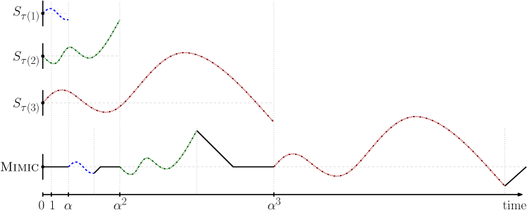
Figure 1: An example execution of algorithm $\textsc{Mimic}(1,0)$ applied for the TRP problem (i.e., we use $\alpha=3$). We assume that $\min(\mathcal{I})=1$. Within time interval $[\tau(k)=\alpha^{k},2\cdot\alpha^{k})$ of phase $k+1$, Mimic executes a $\tau(k)$-schedule $S_{\tau(k)}$ that optimizes function $\textsc{val}_{\tau(k)}$. Afterwards within time interval $[2\cdot\alpha^{k},\tau(k+1)=3\cdot\alpha^{k})$, Mimic resets its state to the initial one (the server of TRP returns to the origin).

3 Intermediate Algorithm DISC

As mentioned in the introduction, we introduce an additional intermediate algorithm Disc, whose analysis will allow us to bound the competitive ratios of both our deterministic and randomized solution. For an integer $\ell$, we use $[\ell]$ to denote the set $\{0,\ldots,\ell-1\}$.

$\textsc{Disc}(\gamma,M,\beta)$ solves the $\gamma$-resettable scheduling problem, and is additionally parameterized by a positive integer $M$, and a real number $\beta\in(0,1/M]$. $\textsc{Disc}(\gamma,M,\beta)$ first chooses a random integer $m\in[M]$. Then, it executes $\textsc{Mimic}(\gamma,\omega=-1+m/M+\beta)$. The main result of this paper is the following bound, whose proof is will be given in the next two sections.

Theorem 3.1.

For any $\gamma$, any positive integer $M$, and any $\beta\in(0,1/M]$, the competitive ratio of $\textsc{Disc}(\gamma,M,\beta)$ for the $\gamma$-resettable scheduling is at most $1+(1/M)\cdot\sum_{j=1}^{M}(2+\gamma)^{j/M}$.

Corollary 3.2.

For any $\gamma$, the competitive ratio of our Mimic-based deterministic solution is at most $3+\gamma$ and the ratio of randomized one at most $1+(1+\gamma)/\ln(2+\gamma)$.

Proof 3.3.

Let $\xi_{M}=1+(1/M)\cdot\sum_{j=1}^{M}\alpha^{j/M}$. First, we note that $\textsc{Disc}(\gamma,M=1,\beta=1)$ chooses deterministically $m=0$ and executes $\textsc{Mimic}(\gamma,\omega=-1+0+1=0)$, i.e., is equivalent to our deterministic algorithm. Hence, by Theorem 3.1, the corresponding competitive ratio is at most $\xi_{1}=3+\gamma$.

For analyzing our randomized algorithm, we observe that instead of choosing a random $\omega\in(-1,0]$, we may choose a random integer $m\in[M]$ and a random real $\beta\in(0,1/M]$ and set $\omega=-1+m/M+\beta$. Thus, for any fixed integer $M$, our randomized algorithm is equivalent to choosing random $\beta\in(0,1/M]$ and running $\textsc{Disc}(\gamma,M,\beta)$.

Fix any input $\mathcal{I}$. By Theorem 3.1, $\mathbf{E}_{m}[\textsc{cost}_{\textsc{Disc}(\gamma,M,\beta)}(\mathcal{I})]\leq\xi_{M}\cdot\textsc{cost}_{\textsc{Opt}}(\mathcal{I})$ holds for any $\beta\in(0,1/M]$, where the expected value is taken over random choice of $m$. Clearly, this relation holds also when $\beta$ is chosen randomly, i.e., $\mathbf{E}_{\omega}[\textsc{cost}_{\textsc{Mimic}(\gamma,\omega)}]=\mathbf{E}_{\gamma}\mathbf{E}_{m}[\textsc{cost}_{\textsc{Disc}(\gamma,M,\beta)}(\mathcal{I})]\leq\xi_{M}\cdot\textsc{cost}_{\textsc{Opt}}(\mathcal{I})$. As the bound is valid for any $M$, and the competitive ratio of our randomized algorithm is at most $\inf_{M\in\mathbb{N}}\{\xi_{M}\}=\lim_{M\to\infty}\xi_{M}=1+(1+\gamma)/\ln(2+\gamma)$.

4 Structural Properties of DISC

In this section, we build relations useful for analyzing the performance of $\textsc{Disc}(\gamma,M,\beta)$ on any instance $\mathcal{I}$ of the $\gamma$-resettable scheduling problem.

We start by presenting structural properties of schedules $S_{\tau}$. We note that even if there exists a $\tau$-schedule $A$ that completes all jobs from $\mathcal{I}$, $S_{\tau}$ may leave some jobs untouched. However, a sufficiently long schedule $S_{\tau}$ completes all jobs.

Lemma 4.1.

Fix any input $\mathcal{I}$. There exists a value $T_{\mathcal{I}}$, such that for any $\tau\geq T_{\mathcal{I}}$, $S_{\tau}$ completes all jobs of $\mathcal{I}$ and is an optimal (cost-minimal) solution for $\mathcal{I}$.

Proof 4.2.

Let Opt be a cost-optimal schedule for $\mathcal{I}$ and let $t$ be its length. Let $w$ be the weight of the lightest job from $\mathcal{I}$. We fix $T_{\mathcal{I}}=\max\{t,(\textsc{val}_{t}(\textsc{Opt})+1)/w\}$. Now, we pick any $\tau\geq T_{\mathcal{I}}$, and investigate properties of $S_{\tau}$.

As $\tau\geq T_{\mathcal{I}}\geq t$, the schedule of Opt can be trivially extended to a $\tau$-schedule $A$ that does nothing in its suffix of length $\tau-t$. Both $A$ and Opt complete all jobs, and thus $\textsc{val}_{\tau}(A)=\textsc{val}_{t}(\textsc{Opt})$. Moreover, as $S_{\tau}$ minimizes function $\textsc{val}_{\tau}$, $\textsc{val}_{\tau}(S_{\tau})\leq\textsc{val}_{\tau}(A)=\textsc{val}_{t}(\textsc{Opt})<T_{\mathcal{I}}\cdot w\leq\tau\cdot w$, and thus $S_{\tau}$ completes all jobs (as otherwise $\textsc{val}_{\tau}$ would include a penalty of at least $\tau\cdot w$). As $S_{\tau}$ and Opt complete all jobs, $\textsc{cost}_{S_{\tau}}(\mathcal{I})=\textsc{val}_{\tau}(S_{\tau})\leq\textsc{val}_{t}(\textsc{Opt})=\textsc{cost}_{\textsc{Opt}}(\mathcal{I})$, i.e., $S_{\tau}$ is an optimal solution for $\mathcal{I}$.

Sub-phases.

Recall that the algorithm $\textsc{Disc}(\gamma,M,\beta)$ chooses a random integer $m\in[M]$, and executes $\textsc{Mimic}(\gamma,\omega=-1+m/M+\beta)$. To compare Disc executions for different random choices, we introduce sub-phases. Recall that $\alpha=2+\gamma$; let $\delta=\alpha^{1/M}$.

Recall that the $k$-th phase of Mimic starts at time $\tau_{k-1}$ and ends at time $\tau_{k}$, where $\tau_{k}=\min(\mathcal{I})\cdot\alpha^{k-1+m/M+\beta}=\min(\mathcal{I})\cdot\alpha^{\beta-1}\cdot\delta^{m+k\cdot M}$. For any $q$, we define

$$\eta_{q}=\eta(q)=\min(\mathcal{I})\cdot\alpha^{\beta-1}\cdot\delta^{q}.$$ (3)

In these terms, $\tau_{k}=\eta_{m+k\cdot M}$. We define the $q$-th sub-phase (for $q\geq 0$) as the time interval starting at time $\eta_{q-1}$ and ending at time $\eta_{q}$. Then, phase $k$ of $\textsc{Disc}(\gamma,M,\beta)$ consists of exactly $M$ sub-phases, numbered from $(k-1)\cdot M+m+1$ to $k\cdot M+m$. An example of phases and sub-phases is given in Figure 2. We emphasize that the start and the end of a sub-phase is a deterministic function of the parameters of Disc, while the start and end of a phase depend additionally on the value $m\in[M]$ that Disc chooses randomly.

Recall that our deterministic algorithm is equivalent to $\textsc{Mimic}(\gamma,0)\equiv\textsc{Disc}(\gamma,1,1)$. In this case $m=0$, and thus $\eta_{q}=\tau_{q}$ for any $q$, i.e., each phase consists of one sub-phase, and their indexes coincide.

Sub-phases vs Auxiliary Schedules.

We now identify the times when auxiliary schedules are computed by $\textsc{Disc}(\gamma,M,\beta)$. Recall that at the beginning of any phase $k+1$ (where $k\geq 1$), i.e., at time $\tau_{k}=\eta_{m+k\cdot M}$, Disc computes and executes schedule $S_{\eta(m+k\cdot M)}$. Let $T_{\mathcal{I}}$ be the threshold guaranteed by 4.1 and we define $K_{\mathcal{I}}$ as the smallest integer satisfying $\eta({K_{\mathcal{I}}\cdot M})\geq T_{\mathcal{I}}$. Note that $K_{\mathcal{I}}$ is a deterministic function of input $\mathcal{I}$.

For any choice of $m\in[M]$, the schedule $S_{\eta(m+K_{\mathcal{I}}\cdot M)}$ completes all jobs. This schedule is executed by Disc in phase $K_{\mathcal{I}}+1$, and thus Disc terminates latest in phase $K_{\mathcal{I}}+1$. Summing up, $\textsc{Disc}(\gamma,M,\beta)$ executes schedules $S_{\eta(m+M)},S_{\eta(m+2M)},\dots,S_{\eta(m+K_{\mathcal{I}}\cdot M)}$. At the beginning of the first phase, Disc does nothing, but for notational ease, we assume that in the first phase, it also computes and executes a dummy schedule $S_{\eta(m)}$, which does not complete any job. For succinctness, we use $A_{q}=S_{\eta(q)}$. In these terms, $\textsc{Disc}(\gamma,M,\beta)$ executes schedules $A_{m+k\cdot M}$ for $k\in[K_{\mathcal{I}}+1]$.

Let $Q=K_{\mathcal{I}}\cdot M+(M-1)$: possible schedule indexes used by Disc range from $0$ to $Q$. For any schedule $A_{q}$, we define the set of indexes of preceding schedules $P(q)=\{q^{\prime},q^{\prime}+M,\ldots,q-M\}$, where $q^{\prime}=q\mod M$.

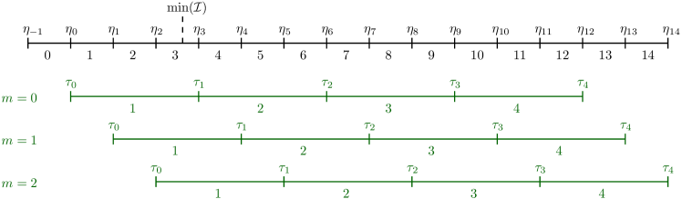
Figure 2: Example of phases (green) and sub-phases (black) of algorithm $\textsc{Disc}(\gamma,M=3,\beta)$ for all possible choices of $m$. The time interval lengths are in logarithmic scale. The starts and ends of sub-phases are deterministic functions of $\gamma$, $M$, and $\beta$, but the start of a phase depends additionally on the integer $m\in[M]$ chosen randomly by Disc. Sub-phase $0$ is not contained in any phase, but will be used in our analysis.

Fresh and Stale Requests.

We assume that no jobs are completed by the online algorithm while it is resetting the executor, and we assume that the execution of schedule $A_{q}$ may complete only jobs from set $R(A_{q})$. It is however important to note that $R(A_{q})$ and $R(A_{q-M})$ may overlap significantly, in which case the execution of schedule $A_{q}$ serves only these jobs from $R(A_{q})$ that have not been served already. To further quantify this effect, for $q\in[Q+1]$, we define the set of fresh jobs of schedule $A_{q}$ as

$$\textstyle R^{\mathrm{F}}(A_{q})=R(A_{q})\setminus\bigcup_{\ell\in P(q)}R(A_{\ell}).$$ (4)

The remaining jobs from $R(A_{q})$ are called stale and are denoted $R^{\mathrm{S}}(A_{q})=R(A_{q})\setminus R^{\mathrm{F}}(A_{q})$. For succinctness, we define the following shorthand notations for their weights:

$$w^{\mathrm{F}}_{q}=w(R^{\mathrm{F}}(A_{q})), w^{\mathrm{S}}_{q}=w(R^{\mathrm{S}}(A_{q})), w_{q}=w(R(A_{q}))=w^{\mathrm{F}}_{q}+w^{\mathrm{S}}_{q}.$$ (5)

Lemma 4.3.

For any $q\in[Q+1]$, it holds that $w^{\mathrm{S}}_{q}\leq\sum_{\ell\in P(q)}w^{\mathrm{F}}_{\ell}$. This relation becomes equality for $q\geq K_{\mathcal{I}}\cdot M$.

Proof 4.4.

By a simple induction, it can be shown that $\biguplus_{\ell\in P(q)}R^{\mathrm{F}}(A_{\ell})=\bigcup_{\ell\in P(q)}R(A_{\ell})$ for any $q\in[Q+1]$. Then, using the definition of stale jobs, $R^{\mathrm{S}}(A_{q})\subseteq\bigcup_{\ell\in P(q)}R(A_{\ell})=\biguplus_{\ell\in P(q)}R^{\mathrm{F}}(A_{\ell})$. Applying weight to both sides yields $w^{\mathrm{S}}_{q}\leq\sum_{\ell\in P(q)}w^{\mathrm{F}}_{\ell}$.

Next, we show that this relation can be reversed for $q\geq K_{\mathcal{I}}\cdot M$ (i.e., for the schedule executed in the last phase of Disc). For such $q$, $A_{q}$ completes all jobs, and thus $\bigcup_{\ell\in P(q)}R(A_{\ell})\subseteq R(A_{q})=R^{\mathrm{F}}(A_{q})\uplus R^{\mathrm{S}}(A_{q})$. By the definition of fresh jobs, $R^{\mathrm{F}}(A_{q})$ does not contain any job from $\bigcup_{\ell\in P(q)}R(A_{\ell})$, and thus $\bigcup_{\ell\in P(q)}R(A_{\ell})\subseteq R^{\mathrm{S}}(A_{q})$. This implies that $\biguplus_{\ell\in P(q)}R^{\mathrm{F}}(A_{\ell})=\bigcup_{\ell\in P(q)}R(A_{\ell})\subseteq R^{\mathrm{S}}(A_{q})$. After applying weights to both sides, we obtain $w^{\mathrm{S}}_{q}\geq\sum_{\ell\in P(q)}w^{\mathrm{F}}_{\ell}$ as desired.

Jobs Completed in Sub-phases.

For further analysis, we refine our notions when a job is completed. For a $\eta_{q}$-schedule $A_{q}$, let $R_{j}(A_{q})$ be the set of jobs completed in sub-phase $j\leq q$, i.e., within interval $[\eta_{j-1},\eta_{j})$. As $\eta_{-1}\leq\eta_{m-1}\leq\min(\mathcal{I})$ (cf. (3)), no job can be completed within the interval $[0,\eta_{-1})$ (before sub-phase $0$). Hence, $R(A_{q})=\biguplus_{j=0}^{q}R_{j}(A_{q})$.

We partition sets $R^{\mathrm{F}}(A_{q})$ and $R^{\mathrm{S}}(A_{q})$ analogously, defining sets $R^{\mathrm{F}}_{j}(A_{q})$ and $R^{\mathrm{S}}_{j}(A_{q})$ (for $0\leq j\leq q$), such that $R^{\mathrm{F}}(A_{q})=\biguplus_{j=0}^{q}R^{\mathrm{F}}_{j}(A_{q})$ and $R^{\mathrm{S}}(A_{q})=\biguplus_{j=0}^{q}R^{\mathrm{S}}_{j}(A_{q})$. For succinctness, for $0\leq j\leq q$, we introduce the following shorthand notations:

• $w^{\mathrm{F}}_{qj}=w(R^{\mathrm{F}}_{j}(A_{q}))$, $w^{\mathrm{S}}_{qj}=w(R^{\mathrm{S}}_{j}(A_{q}))$, and $w_{qj}=w(R_{j}(A_{q}))=w^{\mathrm{F}}_{qj}+w^{\mathrm{S}}_{qj}$;

• $g^{\mathrm{F}}_{qj}=\textsc{cost}_{A_{q}}(R^{\mathrm{F}}_{j}(A_{q}))$, $g^{\mathrm{S}}_{qj}=\textsc{cost}_{A_{q}}(R^{\mathrm{S}}_{j}(A_{q}))$, and $g_{qj}=\textsc{cost}_{A_{q}}(R_{j}(A_{q}))=g^{\mathrm{F}}_{qj}+g^{\mathrm{S}}_{qj}$.

Lemma 4.5.

For any $0\leq q<\ell\leq Q$, it holds that $\sum_{j=0}^{q}(g_{qj}-g_{\ell j})+\sum_{j=0}^{q}\eta_{q}\cdot(w_{\ell j}-w_{qj})\leq 0$.

Proof 4.6.

For any $\eta_{q}$-schedule $B$, it holds that

$$\textsc{val}_{\eta(q)}(B) =\textsc{cost}_{B}(R(B))+\eta_{q}\cdot w\left(\mathcal{I}_{\eta(q)}\setminus R(B)\right)$$

$$\textstyle=\sum_{j=0}^{q}\textsc{cost}_{B}(R_{j}(B))+\eta_{q}\cdot w(\mathcal{I}_{\eta(q)})-\eta_{q}\cdot\sum_{j=0}^{q}w(R_{j}(B)).$$

Fix any $\ell\leq Q$ and let $A^{q}_{\ell}$ be the $\eta_{q}$-schedule consisting of the first $q$ sub-phases of $\eta_{\ell}$-schedule $A_{\ell}$. Since $A_{q}$ is a minimizer of $\textsc{val}_{\eta(q)}$, it holds that $\textsc{val}_{\eta(q)}(A_{q})\leq\textsc{val}_{\eta(q)}(A^{q}_{\ell})$. Thus, $\sum_{j=0}^{q}g_{qj}-\eta_{q}\cdot\sum_{j=0}^{q}w_{qj}\leq\sum_{j=0}^{q}g_{\ell j}-\eta_{q}\cdot\sum_{j=0}^{q}w_{\ell j}.$

Costs of DISC and OPT.

Finally, we can express costs of Disc and Opt using the newly introduced notions.

Lemma 4.7.

For any input $\mathcal{I}$, parameters $M$ and $\beta\in(0,1/M]$, it holds that $\mathbf{E}[\textsc{cost}_{\textsc{Disc}}(\mathcal{I})]$ $=(1/M)\cdot\sum_{q=0}^{Q}\sum_{j=0}^{q}\left(\eta_{q}\cdot w^{\mathrm{F}}_{qj}+g^{\mathrm{F}}_{qj}\right)$.

Proof 4.8.

Recall that Disc chooses random $m\in[M]$ and then at time $\eta_{q}$ it executes schedule $A_{q}$, for all $q\in\{m,m+M,\dots,m+K_{\mathcal{I}}\cdot M\}$. When Disc executes $A_{q}$, it completes jobs from $R^{\mathrm{F}}(A_{q})$. By the delayed execution property of the resettable scheduling (cf. subsection 1.2), each job $r\in R^{\mathrm{F}}(A_{q})$ is completed at time $\eta_{q}+s_{A_{q}}(r)$. Thus, the cost of executing $A_{q}$ by Disc is equal to

$$\textstyle\sum_{r\in R^{\mathrm{F}}(A_{q})}w(r)\cdot(\eta_{q}+s_{A_{q}}(r)) =\eta_{q}\cdot w(R^{\mathrm{F}}(A_{q}))+\textsc{cost}_{A_{q}}(R^{\mathrm{F}}(A_{q}))$$

$$\textstyle=\eta_{q}\cdot w^{\mathrm{F}}_{q}+\sum_{j=0}^{q}g^{\mathrm{F}}_{qj}=\sum_{j=0}^{q}\left(\eta_{q}\cdot w^{\mathrm{F}}_{qj}+g^{\mathrm{F}}_{qj}\right).$$

For any $q\in[Q+1]$, the probability that Disc executes $A_{q}$ is equal to $1/M$, and thus the lemma follows.

Lemma 4.9.

For any input $\mathcal{I}$ and any $q\in\{Q-M+1,Q-M+2,\dots,Q\}$, it holds that $\textsc{cost}_{\textsc{Opt}}(\mathcal{I})=\sum_{j=0}^{q}g_{qj}$.

Proof 4.10.

Recall that for such choice of $q$, schedules $A_{q}$ serve all jobs of $\mathcal{I}$ achieving optimal cost. Therefore, $\textsc{cost}_{\textsc{Opt}}(\mathcal{I})=\textsc{cost}_{A_{q}}(R(A_{q}))=\sum_{j=0}^{q}\textsc{cost}_{A_{q}}(R_{j}(A_{q}))=\sum_{j=0}^{q}g_{qj}$.

5 Factor-Revealing Linear Program

Now we show that the Disc-to-Opt cost ratio on an arbitrary input $\mathcal{I}$ can be upper-bounded by a value of a linear (maximization) program.

Assume we fixed $\gamma$ and any input $\mathcal{I}$ to the $\gamma$-resettable scheduling problem. We also fix parameters of Disc: an integer $M$ and $\beta\in(0,1/M]$. These choices imply the values of $Q$ and $\eta_{q}$ for any $q$. This allows us to define the linear program $\mathcal{P}_{\gamma,\mathcal{I},M,\beta}$ whose goal is to maximize

$$\textstyle\sum_{q=0}^{Q}\sum_{j=0}^{q}\eta_{q}\cdot w^{\mathrm{F}}_{qj}+g^{\mathrm{F}}_{qj}$$ (6)

subject to the following constraints:

$$\textstyle\sum_{j=0}^{q}g_{qj}\leq 1 \text{for all}\;Q-M+1\leq q\leq Q$$ (7)

$$\textstyle\sum_{j=0}^{q}w^{\mathrm{S}}_{qj}-\sum_{\ell\in P(q)}\sum_{j=0}^{\ell}w^{\mathrm{F}}_{\ell j}\leq 0 \text{for all}\;0\leq q\leq Q-M$$ (8)

$$\textstyle\sum_{\ell\in P(q)}\sum_{j=0}^{\ell}w^{\mathrm{F}}_{\ell j}-\sum_{j=0}^{q}w^{\mathrm{S}}_{qj}\leq 0 \text{for all}\;Q-M+1\leq q\leq Q$$ (9)

$$\textstyle\sum_{j=0}^{q}(g_{qj}-g_{\ell j})+\sum_{j=0}^{q}\eta_{q}\cdot(w_{\ell j}-w_{qj})\leq 0 \text{for all}\;0\leq q<\ell\leq Q$$ (10)

$$\eta_{j-1}\cdot w^{\mathrm{S}}_{qj}-g^{\mathrm{S}}_{qj}\leq 0 \text{for all}\;0\leq j\leq q\leq Q$$ (11)

$$g^{\mathrm{F}}_{qj}-\eta_{j}\cdot w^{\mathrm{F}}_{qj}\leq 0 \text{for all}\;0\leq j\leq q\leq Q$$ (12)

$$\eta_{j-1}\cdot w^{\mathrm{F}}_{qj}-g^{\mathrm{F}}_{qj}\leq 0 \text{for all}\;0\leq j\leq q\leq Q$$ (13)

and non-negativity of all variables. In (10), we treat $w_{qj}$ and $g_{qj}$ not as variables, but as shorthand notations for $w^{\mathrm{F}}_{qj}+w^{\mathrm{S}}_{qj}$ and $g^{\mathrm{F}}_{qj}+g^{\mathrm{S}}_{qj}$, respectively.

The intuition behind this LP formulation is that instead of creating the whole input $\mathcal{I}$, the adversary only chooses the values of variables $w^{\mathrm{F}}_{qj}$, $w^{\mathrm{S}}_{qj}$, $g^{\mathrm{F}}_{qj}$ and $g^{\mathrm{S}}_{qj}$ that satisfy some subset of inequalities (inequalities that have to be satisfied if these variables were created on the basis of actual input $\mathcal{I}$). This intuition is formalized below.

Lemma 5.1.

Fix any $\gamma$, any input $\mathcal{I}$ for $\gamma$-resettable scheduling, and parameters of Disc: integer $M$ and $\beta\in(0,1/M]$. Then, $\mathbf{E}[\textsc{cost}_{\textsc{Disc}}(\mathcal{I})]/\textsc{cost}_{\textsc{Opt}}(\mathcal{I})\leq P^{*}_{\gamma,\mathcal{I},M,\beta}/M$, where $P^{*}_{\gamma,\mathcal{I},M,\beta}$ is the value of the optimal solution to $\mathcal{P}_{\gamma,\mathcal{I},M,\beta}$.

Proof 5.2.

By scaling all variables by the same value, $\mathcal{P}_{\gamma,\mathcal{I},M,\beta}$ is equivalent to the (non-linear) optimization program $\mathcal{P}^{\prime}_{\gamma,\mathcal{I},M,\beta}$, whose objective is to maximize $(\sum_{q=0}^{Q}\sum_{j=0}^{q}\eta_{q}\cdot w^{\mathrm{F}}_{qj}+g^{\mathrm{F}}_{qj})/\max_{Q-M+1\leq q\leq Q}\sum_{j=0}^{q}g_{qj}$, subject to constraints (8)–(13). In particular, the optimal values of these programs, $P^{*}_{\gamma,\mathcal{I},M,\beta}$ and $P^{\prime*}_{\gamma,\mathcal{I},M,\beta}$ are equal.

Next, we set the values of variables $w^{\mathrm{F}}_{qj}$, $w^{\mathrm{S}}_{qj}$, $g^{\mathrm{F}}_{qj}$ and $g^{\mathrm{S}}_{qj}$ on the basis of input $\mathcal{I}$, and parameters $M$ and $\beta$. (Note that the variables depend on these parameters, but not on the random choices of Disc.) We now show that they satisfy the constraints of $\mathcal{P}^{\prime*}_{\gamma,\mathcal{I},M,\beta}$ and we relate $\mathbf{E}[\textsc{cost}_{\textsc{Disc}}(\mathcal{I})]/\textsc{cost}_{\textsc{Opt}}(\mathcal{I})$ to $P^{*}_{\gamma,\mathcal{I},M,\beta}$.

By 4.3 and the relations $w^{\mathrm{F}}_{q}=\sum_{j=0}^{q}w^{\mathrm{F}}_{qj}$ and $w^{\mathrm{S}}_{q}=\sum_{j=0}^{q}w^{\mathrm{S}}_{qj}$, the variables satisfy (8) and (9). Next, 4.5 implies (10). Inequalities (11), (12) and (13) follow directly by the definition of costs and weights. Finally, by 4.7 and 4.9, for any $q\in\{Q-M+1,\dots,Q\}$, it holds that $\mathbf{E}[\textsc{cost}_{\textsc{Disc}}(\mathcal{I})]/\textsc{cost}_{\textsc{Opt}}(\mathcal{I})=(1/M)\cdot(\sum_{q=0}^{Q}\sum_{j=0}^{q}\eta_{q}\cdot w^{\mathrm{F}}_{qj}+g^{\mathrm{F}}_{qj})/(\sum_{j=0}^{q}g_{qj})$, and thus $\mathbf{E}[\textsc{cost}_{\textsc{Disc}}(\mathcal{I})]/\textsc{cost}_{\textsc{Opt}}(\mathcal{I})\leq P^{\prime*}_{\gamma,\mathcal{I},M,\beta}/M=P^{*}_{\gamma,\mathcal{I},M,\beta}/M$.

5.1 Dual Program and Competitive Ratio.

By 5.1, the optimal value of $\mathcal{P}_{\gamma,\mathcal{I},M,\beta}$ is an upper bound on the competitive ratio of Disc. By weak duality, an upper-bound is given by any feasible solution to the dual program $\mathcal{D}_{\gamma,\mathcal{I},M,\beta}$ that we present below.

$\mathcal{D}_{\gamma,\mathcal{I},M,\beta}$ uses variables $\xi_{q},B_{q},C_{q},D_{\ell q},F_{qj},G_{qj}$, and $H_{qj}$, corresponding to inequalities (7)–(13) from $\mathcal{P}_{\gamma,\mathcal{I},M,\beta}$, respectively. In the formulas below, we use $L_{q}=M\cdot K+(q\mod M)$ and $S(q)=\{q+M,q+2\cdot M,\dots,L_{q}-M\}$. For succinctness of the description, we introduce two auxiliary variables for any $0\leq j\leq q\leq Q$:

$$\textstyle U_{qj}=\sum_{\ell=q+1}^{Q}D_{\ell q}-\sum_{\ell=j}^{q-1}D_{q\ell} \textstyle V_{qj}=\sum_{\ell=j}^{q-1}\eta_{\ell}\cdot D_{q\ell}-\sum_{\ell=q+1}^{Q}\eta_{q}\cdot D_{\ell q}.$$ and (14)

The goal of $\mathcal{D}_{\gamma,\mathcal{I},M,\beta}$ is to minimize

$$\textstyle\sum_{q=Q-M+1}^{Q}\xi_{q}$$ (15)

subject to the following constraints (in all of them, we omitted the statement that they hold for all $j\in\{0,\ldots,q\}$):

$$U_{qj}+G_{qj}-H_{qj}\geq 1 \text{for all}\;0\leq q\leq Q-M$$ (16)

$$U_{qj}-F_{qj}\geq 0 \text{for all}\;0\leq q\leq Q-M$$ (17)

$$U_{qj}+G_{qj}-H_{qj}+\xi_{q}\geq 1 \text{for all}\;Q-M+1\leq q\leq Q$$ (18)

$$U_{qj}-F_{qj}+\xi_{q}\geq 0 \text{for all}\;Q-M+1\leq q\leq Q$$ (19)

$$\textstyle V_{qj}+\eta_{j-1}\cdot H_{qj}-\eta_{j}\cdot G_{qj}+C_{L_{q}}-\sum_{\ell\in S(q)}B_{\ell}\geq\eta_{q} \text{for all}\;0\leq q\leq Q-M$$ (20)

$$V_{qj}+\eta_{j-1}\cdot F_{qj}+B_{q}\geq 0 \text{for all}\;0\leq q\leq Q-M$$ (21)

$$V_{qj}-\eta_{j}\cdot G_{qj}+\eta_{j-1}\cdot H_{qj}\geq\eta_{q} \text{for all}\;Q-M+1\leq q\leq Q$$ (22)

$$V_{qj}+\eta_{j-1}\cdot F_{qj}-C_{q}\geq 0 \text{for all}\;Q-M+1\leq q\leq Q$$ (23)

and non-negativity of all variables.

Lemma 5.3.

For any $\gamma$, any input $\mathcal{I}$ for $\gamma$-resettable scheduling, any positive integer $M$, and any $\beta\in(0,1/M]$, there exists a feasible solution to $\mathcal{D}_{\gamma,\mathcal{I},M,\beta}$ of value at most $M+\sum_{j=1}^{M}(2+\gamma)^{j/M}$.

We defer the proof to the next subsection, first arguing how it implies the main theorem of the paper (the competitive ratio of Disc).

Proof 5.4 (Proof of Theorem 3.1).

Fix any $\gamma$, and consider algorithm $\textsc{Disc}(\gamma,M,\beta)$ for any positive integer $M$, and any $\beta\in(0,1/M]$. Fix any input $\mathcal{I}$ to the $\gamma$-resettable scheduling problem. Let $P^{*}_{\gamma,\mathcal{I},M,\beta}$ be the value of an optimal solution to $\mathcal{P}_{\gamma,\mathcal{I},M,\beta}$. By weak duality and 5.3, $P_{\gamma,\mathcal{I},M,\beta}\leq M+\sum_{j=1}^{M}(2+\gamma)^{j/M}$. Hence, by 5.1, $\mathbf{E}[\textsc{cost}_{\textsc{Disc}}(\mathcal{I})]/\textsc{cost}_{\textsc{Opt}}(\mathcal{I})\leq P^{*}_{\gamma,\mathcal{I},M,\beta}/M\leq 1+(1/M)\cdot\sum_{j=1}^{M}(2+\gamma)^{j/M}$, as desired.

5.2 Proof of 5.3

Let

$$\textstyle\Delta_{k}=\sum_{i=0}^{k}\delta^{i}=\left(\delta^{k+1}-1\right)/\left(\delta-1\right).$$

In particular $\Delta_{-1}=0$. We choose the following values of the dual variables:

$$\xi_{q}=1+\delta^{q-Q+M}\quad\text{for}\;Q-M+1\leq q\leq Q,$$

$$F_{qj} =\begin{cases}\xi_{q}&\text{for}\;Q-M+1\leq j\leq q\leq Q,\\ \delta\cdot\Delta_{M-1}&\text{for}\;0\leq j\leq Q-M\text{ and }q=j,\\ 1&\text{for}\;0\leq j\leq Q-M\text{ and }q\in\{j+1,\ldots,j+M\},\\ 0&\text{otherwise},\end{cases}$$

$$G_{qj} =\begin{cases}\Delta_{q-Q+M-1}-\Delta_{q-j}&\text{for}\;Q-M+1\leq j\leq q\leq Q,\\ \Delta_{q-j-M-1}&\text{for}\;j\leq q-M\\ 0&\text{otherwise},\end{cases}$$

$$B_{q} =\eta_{q-M-1}\cdot\left(\delta^{M+1}+1\right)\cdot\left(\delta^{M}-1\right) \text{for}\;0\leq q\leq Q-M,$$

$$C_{q} =\eta_{q-M-1}\cdot\left(\delta^{M+1}+1\right) \text{for}\;Q-M+1\leq q\leq Q,$$

$$D_{qj} =F_{q,j+1}-F_{qj} \text{for}\;0\leq j<q\leq Q,$$

$$H_{qj} =F_{qj}+G_{qj}-1 \text{for}\;0\leq j\leq q\leq Q.$$

The values of $F_{qj}$ and $G_{qj}$ (for $0\leq j\leq q\leq Q)$ are depicted in Figure 3 for an easier reference. We will extensively use the property that $\eta_{i}\cdot\delta^{j}=\eta_{i+j}$ for any $i$ and $j$.

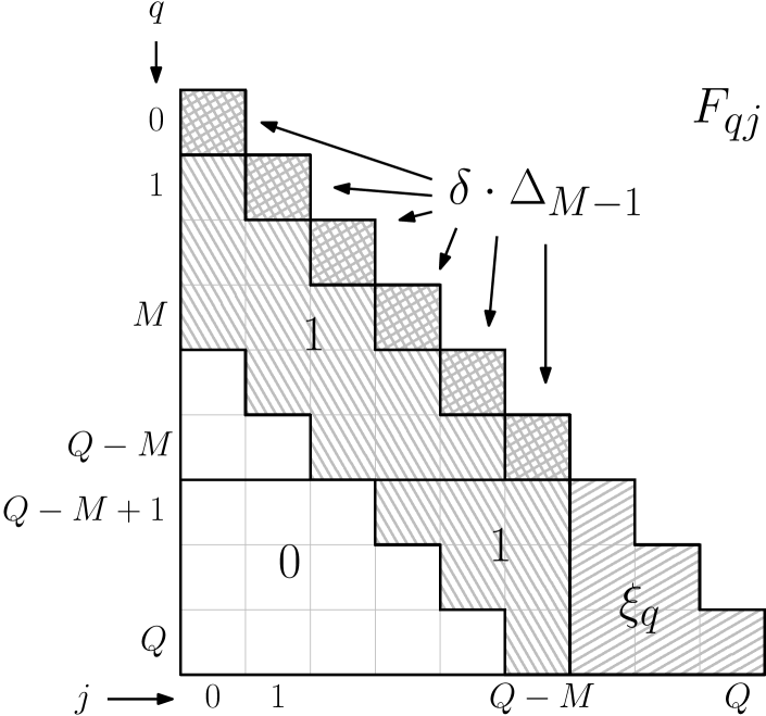
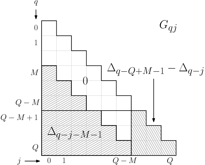
Figure 3: Visual presentation of values assigned to dual variables $F_{qj}$ (left) and $G_{qj}$ (right) for $M=3$ and $Q=8$.

Objective Value.

With the above assignment of dual variables the objective value of $\mathcal{D}_{\gamma,\mathcal{I},M,\beta}$ is equal to $\sum_{q=Q-M+1}^{Q}\xi_{q}=M+\sum_{j=1}^{M}\delta^{j}=M+\sum_{j=1}^{M}(2+\gamma)^{j/M}$ as desired.

Non-negativity of Variables.

Variables $\xi_{q},C_{q},B_{q},F_{qj}$ and $G_{qj}$ are trivially non-negative (for those $q$ and $j$ for which they are defined). The non-negativity of $D_{qj}=F_{q,j+1}-F_{qj}$ follows as $F_{qj}$ is a non-decreasing function of its second argument (cf. Figure 3).

Finally, for showing non-negativity of variable $H_{qj}$, we consider two cases. If $j\geq q-M$, then $F_{qj}\geq 1$. Otherwise, $j\leq q-M-1$, and then $G_{qj}=\Delta_{q-j-M-1}\geq 1$. Thus, in either case $H_{qj}=F_{qj}+G_{qj}-1\geq 0$.

Helper Bounds.

It remains to show that the given values of dual variables satisfy all constraints (16)–(23) of the dual program $\mathcal{D}_{\gamma,\mathcal{I},M,\beta}$. We define a few helper notions and identities that are used throughout the proof of dual feasibility. For any $q\in[Q+1]$, let

$$\textstyle R_{q}=\sum_{\ell=q+1}^{Q}D_{\ell q}=\sum_{\ell=q+1}^{Q}\left(F_{\ell,q+1}-F_{\ell q}\right).$$

Lemma 5.5.

$R_{q}=\delta\cdot\Delta_{M-1}$ for $q\leq Q-M$ and $R_{q}=0$ otherwise.

Proof 5.6.

We consider three cases.

1. $q\in\{0,\dots,Q-M-1\}$. Then, $R_{q}=F_{q+1,q+1}+\sum_{\ell=q+1}^{Q}\left(F_{\ell+2,\ell+1}-F_{\ell+1,\ell}\right)-F_{Qq}=\delta\cdot\Delta_{M-1}+\sum_{\ell=q+1}^{Q}0-0=\delta\cdot\Delta_{M-1}$.

2. $q=Q-M$. Then, $R_{q}=\sum_{\ell=Q-M+1}^{Q}(\xi_{\ell}-1)=\sum_{j=1}^{M}\delta^{j}=\delta\cdot\Delta_{M-1}$.

3. $q\in\{Q-M+1,\dots,Q\}$. Then, $R_{q}=\sum_{\ell=q+1}^{Q}(\xi_{\ell}-\xi_{\ell})=0$.

Next, we investigate the values of $V_{qj}$ for different $q$ and $j$. Using its definition (cf. (14)),

$$\textstyle V_{qj}=\sum_{\ell=j}^{q-1}\eta_{\ell}\cdot D_{q\ell}-\sum_{\ell=q+1}^{Q}\eta_{q}\cdot D_{\ell q}=\sum_{\ell=j}^{q-1}\eta_{\ell}\cdot\left(F_{q,\ell+1}-F_{q\ell}\right)-\eta_{q}\cdot R_{q}.$$ (24)

Additionally, using $H_{qj}=F_{qj}+G_{qj}-1$, we obtain

$$\eta_{j}\cdot G_{qj}-\eta_{j-1}\cdot H_{qj}=(\eta_{j}-\eta_{j-1})\cdot G_{qj}+\eta_{j-1}-\eta_{j-1}\cdot F_{qj}.$$ (25)

Using the chosen values of $G_{qj}$, we observe that

$$(\eta_{j}-\eta_{j-1})\cdot G_{qj}=\begin{cases}\eta_{q+j-Q+M-1}-\eta_{q}&\text{for}\;Q-M+1\leq j\leq q,\\ \eta_{q-M-1}-\eta_{j-1}&\text{for}\;j\leq q-M-1,\\ 0&\text{otherwise}.\end{cases}$$ (26)

Furthermore, in all the cases, it can be verified that

$$(\eta_{j}-\eta_{j-1})\cdot G_{qj}+\eta_{j-1}-\eta_{q-M-1}\geq 0.$$ (27)

5.2.1 Showing inequalities (16)–(19)

We prove that relations (16)–(19) hold with equality. In fact, it suffices to show (17) and (19): inequalities (16) and (18) follow immediately as we chose $H_{qj}=F_{qj}+G_{qj}-1$. Using the definition of $U_{qj}$ (cf. (14)), we obtain

$$\textstyle U_{qj}=\sum_{\ell=q+1}^{Q}D_{\ell q}-\sum_{\ell=j}^{q-1}D_{q\ell}=R_{q}-\sum_{\ell=j}^{q-1}\left(F_{q,\ell+1}-F_{q\ell}\right)=R_{q}-F_{qq}+F_{qj}.$$

Now, we observe that for $q\leq Q-M$, it holds that $R_{q}-F_{qq}=\delta\cdot\Delta_{M-1}-\delta\cdot\Delta_{M-1}=0$, and thus $U_{qj}-F_{qj}=0$, which implies (17). On the other hand, for $q>Q-M$, it holds that $R_{q}-F_{qq}=0-\xi_{q}$, and hence $U_{qj}-F_{qj}+\xi_{q}=0$, which implies (19).

5.2.2 Showing inequalities (20)–(21)

Within this part, we assume $q\leq Q-M$. We start with evaluating some terms that are present in (20) and (21). First, we observe that

$$B_{q}=\eta_{q-M-1}\cdot\left(\delta^{M+1}+1\right)\cdot\left(\delta^{M}-1\right)=\eta_{q+M}-\eta_{q}+\eta_{q-1}-\eta_{q-M-1}.$$ (28)

Second, we compute the term $C_{L_{q}}-\sum_{\ell\in S(q)}B_{\ell}$. Recall that $S(q)=\{q+M,q+2\cdot M,\dots,L_{q}-M\}$. Thus,

$$\textstyle C_{L_{q}}-\sum_{\ell\in S(q)}B_{\ell} =\textstyle\left(\delta^{M+1}+1\right)\cdot\left[\eta(L_{q}-M-1)-(\delta^{M}-1)\cdot\eta(-M-1)\cdot\sum_{\ell\in S(q)}\delta^{\ell}\right]$$

$$=(\delta^{M+1}+1)\cdot\left[\eta(L_{q}-M-1)-\eta(-M-1)\cdot\left(\delta^{L_{q}}-\delta^{q+M}\right)\right]$$

$$=(\delta^{M+1}+1)\cdot\eta_{q-1}=\eta_{q+M}+\eta_{q-1}.$$ (29)

Lemma 5.7.

Fix any $0\leq j\leq q\leq Q-M$. Then,

$$V_{qj}=\eta_{q}-\eta_{q-1}-\eta_{q+M}-\eta_{j-1}\cdot F_{qj}+(\eta_{j}-\eta_{j-1})\cdot G_{qj}+\eta_{j-1}.$$

Proof 5.8.

By the definition, $\Delta_{M-1}=\sum_{i=0}^{M-1}\delta^{i}$, and therefore $(\eta_{q-1}-\eta_{q})\cdot\delta\cdot\Delta_{M-1}=\eta_{q}-\eta_{q+M}$. Thus, it suffices to show the following relation

$$V_{qj}=\eta_{q-1}\cdot(\delta\cdot\Delta_{M-1}-1)-\eta_{q}\cdot\delta\cdot\Delta_{M-1}-\eta_{j-1}\cdot F_{qj}+(\eta_{j}-\eta_{j-1})\cdot G_{qj}+\eta_{j-1}.$$

To evaluate $V_{qj}$ using (24), it is useful to trace values $F_{qj},F_{q,j+1},\dots,F_{qq}$ (cf. Figure 3), noting that only the increases of these values contribute to $V_{qj}$. We also note that for $q\leq Q-M$, possible increases are from $0$ to $1$ (between $F_{q,q-M-1}$ and $F_{q,q-M}$) and from $1$ to $\delta\cdot\Delta_{M-1}$ (between $F_{q,q-1}$ and $F_{qq}$). We consider three cases, using $R_{q}=\delta\cdot\Delta_{M-1}$ below.

1. $j\leq q-M-1$. Then, $F_{qj}=0$ and

   $$V_{qj} =\eta_{q-1}\cdot\left(F_{qq}-F_{q,q-1}\right)+\eta_{q-M-1}\cdot\left(F_{q,q-M}-F_{q,q-M-1}\right)-\eta_{q}\cdot R_{q}$$

   $$=\eta_{q-1}\cdot\left(\delta\cdot\Delta_{M-1}-1\right)-\eta_{q}\cdot\delta\cdot\Delta_{M-1}+\eta_{q-M-1}-\eta_{j-1}+\eta_{j-1}-\eta_{j-1}\cdot F_{qj}.$$

   The lemma follows as $(\eta_{j}-\eta_{j-1})\cdot G_{qj}=\eta_{q-M-1}-\eta_{j-1}$ (see (26)).

2. $j\in\{q-M,\ldots,q-1\}$. Then $F_{qj}=1$, and

   $$V_{qj} =\eta_{q-1}\cdot\left(F_{qq}-F_{q,q-1}\right)-\eta_{q}\cdot R_{q}$$

   $$=\eta_{q-1}\cdot\left(\delta\cdot\Delta_{M-1}-1\right)-\eta_{q}\cdot\delta\cdot\Delta_{M-1}$$

   $$=\eta_{q-1}\cdot\left(\delta\cdot\Delta_{M-1}-1\right)-\eta_{q}\cdot\delta\cdot\Delta_{M-1}-\eta_{j-1}\cdot F_{qj}+\eta_{j-1}.$$

   The lemma follows as $(\eta_{j}-\eta_{j-1})\cdot G_{qj}=0$ (see (26)).

3. $j=q$. Then $F_{qj}=\delta\cdot\Delta_{M-1}$, and thus

   $$V_{qj} =-\eta_{q}\cdot R_{q}$$

   $$=\eta_{q-1}\cdot\delta\cdot\Delta_{M-1}-\eta_{q}\cdot\delta\cdot\Delta_{M-1}-\eta_{j-1}\cdot F_{qj}$$

   $$=\eta_{q-1}\cdot\left(\delta\cdot\Delta_{M-1}-1\right)-\eta_{q}\cdot\delta\cdot\Delta_{M-1}-\eta_{j-1}\cdot F_{qj}+\eta_{j-1}.$$

   As in the previous case, the lemma follows as $(\eta_{j}-\eta_{j-1})\cdot G_{qj}=0$.

Showing Inequality (20).

We show that (20) holds with equality. Using 5.7, (29), and (25) yields

$$V_{qj} \textstyle+\eta_{j-1}\cdot H_{qj}-\eta_{j}\cdot G_{qj}+C_{L_{q}}-\sum_{\ell\in S(q)}B_{\ell}$$

$$=\eta_{q}-\eta_{q-1}-\eta_{q+M}-\eta_{j-1}\cdot F_{qj}+(\eta_{j}-\eta_{j-1})\cdot G_{qj}+\eta_{j-1}$$

$$\quad-(\eta_{j}-\eta_{j-1})\cdot G_{qj}-\eta_{j-1}+\eta_{j-1}\cdot F_{qj}+\eta_{q+M}+\eta_{q-1}=\eta_{q}.$$

Showing Inequality (21).

Using 5.7, (29), and (25) yields

$$V_{qj} +\eta_{j-1}\cdot F_{qj}+B_{q}$$

$$=\eta_{q}-\eta_{q-1}-\eta_{q+M}-\eta_{j-1}\cdot F_{qj}+(\eta_{j}-\eta_{j-1})\cdot G_{qj}+\eta_{j-1}$$

$$\quad+\eta_{j-1}\cdot F_{qj}+\eta_{q+M}-\eta_{q}+\eta_{q-1}-\eta_{q-M-1}$$

$$=(\eta_{j}-\eta_{j-1})\cdot G_{qj}+\eta_{j-1}-\eta_{q-M-1}\geq 0.$$

where the last inequality follows by (27).

5.2.3 Showing inequalities (22)–(23)

Within this part, we assume that $q\geq Q-M+1$.

Lemma 5.9.

Fix any $q\geq Q-M+1$ and $0\leq j\leq q$. Then,

$$V_{qj}=\eta_{q}+(\eta_{j}-\eta_{j-1})\cdot G_{qj}-\eta_{j-1}\cdot F_{qj}+\eta_{j-1}.$$

Proof 5.10.

As $g\geq Q-M+1$, it holds that $R_{q}=0$, and thus (24) reduces to

$$\textstyle V_{qj}=\sum_{\ell=j}^{q-1}\eta_{\ell}\cdot\left(F_{q,\ell+1}-F_{q\ell}\right).$$

As in the proof of 5.7, to further evaluate $V_{qj}$, it is useful to trace values $F_{qj},F_{q,j+1},\dots,$ $F_{qq}$ (cf. Figure 3), where the increases of these values contribute to $V_{qj}$. We also note that for $q\geq Q-M+1$, the possible increases are from $0$ to $1$ (between $F_{q,q-M-1}$ and $F_{q,q-M}$) and from $1$ to $\xi_{q}$ (between $F_{q,Q-M}$ and $F_{q,Q-M+1}$). We consider three cases.

1. $j\leq q-M-1$. Then $F_{qj}=0$, and

   $$V_{qj} =\eta_{Q-M}\cdot\left(F_{qq}-F_{q,q-1}\right)+\eta_{q-M-1}\cdot\left(F_{q,q-M}-F_{q,q-M-1}\right)$$

   $$=\eta_{Q-M}\cdot\left(\xi_{q}-1\right)+\eta_{q-M-1}$$

   $$=\eta_{q}+\eta_{q-M-1}-\eta_{j-1}+\eta_{j-1}-\eta_{j-1}\cdot F_{qj}.$$

   The lemma follows as $(\eta_{j}-\eta_{j-1})\cdot G_{qj}=\eta_{q-M-1}-\eta_{j-1}$ (see (26)).

2. $j\in\{q-M,\ldots,Q-M\}$. Then $F_{qj}=1$, and

   $$V_{qj} =\eta_{Q-M}\cdot\left(F_{qq}-F_{q,q-1}\right)$$

   $$=\eta_{Q-M}\cdot\left(\xi_{q}-1\right)$$

   $$=\eta_{q}-\eta_{j-1}\cdot F_{qj}+\eta_{j-1}.$$

   The lemma follows as $(\eta_{j}-\eta_{j-1})\cdot G_{qj}=0$ (see (26)).

3. $j\in\{q-M,\ldots,Q-M\}$. Then $F_{qj}=\xi_{q}=1+\delta^{q-Q+M}$, and

   $$V_{qj}=0 =\eta_{q}+\eta_{q+j-Q+M-1}-\eta_{q}-\eta_{j-1}\cdot(1+\delta^{q-Q+M})+\eta_{j-1}$$

   $$=\eta_{q}+\eta_{q+j-Q+M-1}-\eta_{q}-\eta_{j-1}\cdot F_{qj}+\eta_{j-1}.$$

   The lemma follows as $(\eta_{j}-\eta_{j-1})\cdot G_{qj}=\eta_{q+j-Q+M-1}-\eta_{q}$ (see (26)).

Showing Inequality (22).

We show that (22) holds with equality. Using 5.9 and (25), we obtain

$$V_{qj} \textstyle+\eta_{j-1}\cdot H_{qj}-\eta_{j}\cdot G_{qj}$$

$$=\eta_{q}+(\eta_{j}-\eta_{j-1})\cdot G_{qj}-\eta_{j-1}\cdot F_{qj}+\eta_{j-1}-(\eta_{j}-\eta_{j-1})\cdot G_{qj}-\eta_{j-1}+\eta_{j-1}\cdot F_{qj}$$

$$=\eta_{q}.$$

Showing Inequality (23).

Using 5.9, (25), and the definition of $C_{q}$, we obtain

$$V_{qj} \textstyle+\eta_{j-1}\cdot F_{qj}-C_{q}$$

$$=\eta_{q}+(\eta_{j}-\eta_{j-1})\cdot G_{qj}-\eta_{j-1}\cdot F_{qj}+\eta_{j-1}+\eta_{j-1}\cdot F_{qj}-\eta_{q}-\eta_{q-M-1}$$

$$=(\eta_{j}-\eta_{j-1})\cdot G_{qj}+\eta_{j-1}-\eta_{q-M-1}\geq 0.$$

where the last inequality follows by (27).

6 Tightness of the Analysis

The analysis of our algorithms is tight as proven below. For the deterministic one, we additionally show that choosing $\omega$ different from $0$ does not help.

Theorem 6.1.

For any $\gamma$, there are $\gamma$-resettable scheduling problems, such that for any $\omega\in(-1,0]$, the competitive ratio of $\textsc{Mimic}(\gamma,\omega)$ is at least $3+\gamma$.

Proof 6.2.

We fix a small $\varepsilon>0$ and let $\alpha=2+\gamma$. The input $\mathcal{I}$ contains two jobs: the first one of weight $\varepsilon$ that arrives at time $1$, and second one of weight $1$ that arrives at time $\alpha^{1+\omega}+\varepsilon$. We assume that there exists a schedule $S_{1}$ that serves the first job at the time of its arrival and a schedule $S_{2}$ that serves both jobs at the times of their arrivals. Therefore, $\textsc{cost}_{\textsc{Opt}}(\mathcal{I})=\varepsilon\cdot 1+1\cdot(\alpha^{1+\omega}+\varepsilon)=\alpha^{1+\omega}+2\cdot\varepsilon$.

For analyzing the cost of Mimic, note that at at time $1$, Mimic observes the first job and learns the value of $\min(\mathcal{I})=1$. This is the sole purpose of the first job: setting $\min(\mathcal{I})=1$ makes the algorithm miss the opportunity to serve the second job early. At time $\tau_{1}=\alpha^{1+\omega}$, Mimic executes the $\tau_{1}$-schedule $S^{\prime}_{1}$, which is schedule $S_{1}$ prolonged trivially to length $\tau_{1}$. Next, at time $\tau_{2}=\alpha^{2+\omega}$, Mimic executes the $\tau_{2}$-schedule $S^{\prime}_{2}$, which is schedule $S_{2}$ prolonged trivially to length $\tau_{2}$. This way it completes the second job at time $\tau_{2}+(\alpha^{1+\omega}+\varepsilon)$, and thus $\textsc{cost}_{\textsc{Mimic}}(\mathcal{I})\geq\tau_{2}+\alpha^{1+\omega}+\varepsilon=\alpha^{1+\omega}\cdot(1+\alpha)+\varepsilon$. By taking appropriately small $\varepsilon>0$, the ratio between $\textsc{cost}_{\textsc{Mimic}}(\mathcal{I})$ and $\textsc{cost}_{\textsc{Opt}}(\mathcal{I})$ becomes arbitrarily close to $1+\alpha=3+\gamma$.

Theorem 6.3.

For any $\gamma$, there are $\gamma$-resettable scheduling problems, such that the competitive ratio of a randomized algorithm that runs $\textsc{Mimic}(\gamma,\omega)$ with a random $\omega\in(-1,0]$ is at least $1+(1+\gamma)/\ln(2+\gamma)$.

Proof 6.4.

Let $\alpha=2+\gamma$. The input $\mathcal{I}$ contains a single job of weight $1$ arriving at time $1$. We also assume that for any $\tau\geq 1$, there exists a $\tau$-schedule $S_{\tau}$ that completes this job at time $1$. Clearly, $\textsc{cost}_{\textsc{Opt}}(\mathcal{I})=1\cdot 1=1$.

At time $1$, Mimic observes the only job of $\mathcal{I}$ and learns that $\min(\mathcal{I})=1$. Its sets $\tau_{1}=\alpha^{1+\omega}$ and at time $\tau_{1}$ it executes schedule $S_{\tau_{1}}$, thus completing the job at time $\tau_{1}+1$. Therefore, $\textsc{cost}_{\textsc{Mimic}}(\mathcal{I})=\int_{-1}^{0}\tau_{1}+1\;d\omega=\int_{-1}^{0}\alpha^{1+\omega}+1\;d\omega=1+(\alpha-1)/\ln\alpha=1+(1+\gamma)/\ln(2+\gamma)$. This implies the desired lower bound.

7 Flaw in the Randomized Lower Bound for DARP

The authors of [22] claim a lower bound of $3$ for randomized $k$-DARP (for any $k\geq 1$), see Theorem 4 of [22]. Below we show a flaw in their argument.

The construction given in the proof of their Theorem 4 uses Yao min-max principle and is parameterized with a few variables, in particular with an integer $m$ and with a real number $v\in[0,1]$. Towards the end of the proof, they show that the competitive ratio of any randomized algorithm for the $k$-DARP problem is at least

$$L_{m,v}=\frac{3m-4km-4km^{2}+v^{\frac{m+1}{2-m}}\cdot(3+(4km^{2}+4km+6m+6)\cdot v)}{-4-m-2km-2km^{2}+v^{\frac{m+1}{2-m}}\cdot(3+(2km^{2}+2km+4m+4)\cdot v)}$$

and they claim that there exists $v$, such that $L_{m,v}=3$ when $m$ tends to infinity. However, for any fixed $k$ and any $v$ (also being a function of $m$), by dividing numerator and denominator by $m^{2}$, we obtain that

$$\lim_{m\to\infty}L_{m,v}=\frac{-4k+v^{\frac{m+1}{2-m}}\cdot 4k\cdot v}{-2k+v^{\frac{m+1}{2-m}}\cdot 2k\cdot v}=2.$$

That is, the proven lower bound is $2$ instead of $3$.

References

- [1] Foto N. Afrati, Evripidis Bampis, Chandra Chekuri, David R. Karger, Claire Kenyon, Sanjeev Khanna, Ioannis Milis, Maurice Queyranne, Martin Skutella, Clifford Stein, and Maxim Sviridenko. Approximation schemes for minimizing average weighted completion time with release dates. In Proc. 40th IEEE Symp. on Foundations of Computer Science (FOCS), pages 32–44, 1999. doi:10.1109/SFFCS.1999.814574.
- [2] Sanjeev Arora and George Karakostas. Approximation schemes for minimum latency problems. SIAM Journal on Computing, 32(5):1317–1337, 2003. doi:10.1137/S0097539701399654.
- [3] Norbert Ascheuer, Sven Oliver Krumke, and Jörg Rambau. Online dial-a-ride problems: Minimizing the completion time. In Proc. 17th Symp. on Theoretical Aspects of Computer Science (STACS), pages 639–650, 2000. doi:10.1007/s10951-005-6811-3.
- [4] Giorgio Ausiello, Esteban Feuerstein, Stefano Leonardi, Leen Stougie, and Maurizio Talamo. Serving requests with on-line routing. In Proc. 4th Scandinavian Symposium and Workshops on Algorithm Theory (SWAT), pages 37–48, 1994. doi:10.1007/3-540-58218-5_4.
- [5] Giorgio Ausiello, Esteban Feuerstein, Stefano Leonardi, Leen Stougie, and Maurizio Talamo. Competitive algorithms for the on-line traveling salesman. In Proc. 4th Int. Workshop on Algorithms and Data Structures (WADS), pages 206–217, 1995. doi:10.1007/3-540-60220-8_63.
- [6] Giorgio Ausiello, Esteban Feuerstein, Stefano Leonardi, Leen Stougie, and Maurizio Talamo. Algorithms for the on-line travelling salesman. Algorithmica, 29(4):560–581, 2001. doi:10.1007/s004530010071.
- [7] Ricardo A. Baeza-Yates, Joseph C. Culberson, and Gregory J. E. Rawlins. Searching in the plane. Information and Computation, 106(2):234–252, 1993.
- [8] Marcin Bienkowski and Hsiang-Hsuan Liu. An improved online algorithm for the traveling repairperson problem on a line. In Proc. 44th Int. Symp. on Mathematical Foundations of Computer Science (MFCS), pages 6:1–6:12, 2019. doi:10.4230/LIPIcs.MFCS.2019.6.
- [9] Alexander Birx and Yann Disser. Tight analysis of the smartstart algorithm for online dial-a-ride on the line. SIAM Journal on Discrete Mathematics, 34(2):1409–1443, 2020. doi:10.1137/19M1268513.
- [10] Alexander Birx, Yann Disser, and Kevin Schewior. Improved bounds for open online dial-a-ride on the line. In Approximation, Randomization, and Combinatorial Optimization. Algorithms and Techniques (APPROX/RANDOM), pages 21:1–21:22, 2019. doi:10.4230/LIPIcs.APPROX-RANDOM.2019.21.
- [11] Antje Bjelde, Yann Disser, Jan Hackfeld, Christoph Hansknecht, Maarten Lipmann, Julie Meißner, Kevin Schewior, Miriam Schlöter, and Leen Stougie. Tight bounds for online TSP on the line. In Proc. 28th ACM-SIAM Symp. on Discrete Algorithms (SODA), pages 994–1005, 2017. doi:10.1137/1.9781611974782.63.
- [12] Markus Bläser. Metric TSP. In Encyclopedia of Algorithms, pages 1276–1279. Springer, 2016. doi:10.1007/978-1-4939-2864-4_230.
- [13] Michiel Blom, Sven Oliver Krumke, Willem de Paepe, and Leen Stougie. The online TSP against fair adversaries. INFORMS Journal on Computing, 13(2):138–148, 2001. doi:10.1287/ijoc.13.2.138.10517.
- [14] Vincenzo Bonifaci and Leen Stougie. Online k-server routing problems. Theory of Computing Systems, 45(3):470–485, 2009. doi:10.1007/s00224-008-9103-4.
- [15] Allan Borodin and Ran El-Yaniv. Online Computation and Competitive Analysis. Cambridge University Press, 1998.
- [16] Soumen Chakrabarti, Cynthia A. Phillips, Andreas S. Schulz, David B. Shmoys, Clifford Stein, and Joel Wein. Improved scheduling algorithms for minsum criteria. In Proc. 23rd Int. Colloq. on Automata, Languages and Programming (ICALP), pages 646–657, 1996. doi:10.1007/3-540-61440-0_166.
- [17] Kamalika Chaudhuri, Brighten Godfrey, Satish Rao, and Kunal Talwar. Paths, trees, and minimum latency tours. In Proc. 44th IEEE Symp. on Foundations of Computer Science (FOCS), pages 36–45, 2003. doi:10.1109/SFCS.2003.1238179.
- [18] Pei-Chuan Chen, Erik D. Demaine, Chung-Shou Liao, and Hao-Ting Wei. Waiting is not easy but worth it: the online TSP on the line revisited. Unpublished, 2019. URL: http://arxiv.org/abs/1907.00317.
- [19] José R. Correa and Michael R. Wagner. Lp-based online scheduling: from single to parallel machines. Mathematical Programming, 119(1):109–136, 2009. doi:10.1007/s10107-007-0204-7.
- [20] Willem de Paepe, Jan Karel Lenstra, Jirí Sgall, René A. Sitters, and Leen Stougie. Computer-aided complexity classification of dial-a-ride problems. INFORMS Journal on Computing, 16(2):120–132, 2004. doi:10.1287/ijoc.1030.0052.
- [21] Esteban Feuerstein and Leen Stougie. On-line single-server dial-a-ride problems. Theoretical Computer Science, 268(1):91–105, 2001. doi:10.1016/S0304-3975(00)00261-9.
- [22] Irene Fink, Sven Oliver Krumke, and Stephan Westphal. New lower bounds for online k-server routing problems. Information Processing Letters, 109(11):563–567, 2009. doi:10.1016/j.ipl.2009.01.024.
- [23] R.L. Graham, E.L. Lawler, J.K. Lenstra, and A.H.G.Rinnooy Kan. Optimization and approximation in deterministic sequencing and scheduling: a survey. In Discrete Optimization II, volume 5 of Annals of Discrete Mathematics, pages 287–326. Elsevier, 1979. doi:10.1016/S0167-5060(08)70356-X.
- [24] Leslie A. Hall, Andreas S. Schulz, David B. Shmoys, and Joel Wein. Scheduling to minimize average completion time: Off-line and on-line approximation algorithms. Mathematics of Operations Research, 22(3):513–544, 1997. doi:10.1287/moor.22.3.513.
- [25] Dietrich Hauptmeier, Sven Oliver Krumke, and Jörg Rambau. The online dial-a-ride problem under reasonable load. In Proc. 4th Int. Conf. on Algorithms and Complexity (CIAC), pages 125–136, 2000. doi:10.1007/3-540-46521-9_11.
- [26] Han Hoogeveen, Petra Schuurman, and Gerhard J. Woeginger. Non-approximability results for scheduling problems with minsum criteria. INFORMS Journal on Computing, 13(2):157–168, 2001. doi:10.1287/ijoc.13.2.157.10520.
- [27] Dawsen Hwang and Patrick Jaillet. Online scheduling with multi-state machines. Networks, 71(3):209–251, 2018. doi:10.1002/net.21799.
- [28] Patrick Jaillet and Michael R. Wagner. Online routing problems: Value of advanced information as improved competitive ratios. Transp. Sci., 40(2):200–210, 2006. doi:10.1287/trsc.1060.0147.
- [29] Patrick Jaillet and Michael R. Wagner. Generalized online routing: New competitive ratios, resource augmentation, and asymptotic analyses. Oper. Res., 56(3):745–757, 2008. doi:10.1287/opre.1070.0450.
- [30] Vinay A. Jawgal, V. N. Muralidhara, and P. S. Srinivasan. Online travelling salesman problem on a circle. In Proc. 15th Theory and Applications of Models of Computation (TAMC), pages 325–336, 2019. doi:10.1007/978-3-030-14812-6_20.
- [31] Sven Oliver Krumke, Willem de Paepe, Diana Poensgen, Maarten Lipmann, Alberto Marchetti-Spaccamela, and Leen Stougie. On minimizing the maximum flow time in the online dial-a-ride problem. In Proc. 3rd Workshop on Approximation and Online Algorithms (WAOA), pages 258–269, 2005. doi:10.1007/11671411_20.
- [32] Sven Oliver Krumke, Willem de Paepe, Diana Poensgen, and Leen Stougie. News from the online traveling repairman. Theoretical Computer Science, 295:279–294, 2003. doi:10.1016/S0304-3975(02)00409-7.
- [33] Sven Oliver Krumke, Willem de Paepe, Diana Poensgen, and Leen Stougie. Erratum to "news from the online traveling repairman" [TCS 295 (1-3) (2003) 279-294]. Theoretical Computer Science, 352(1-3):347–348, 2006. doi:10.1016/j.tcs.2005.11.036.
- [34] Sven Oliver Krumke, Luigi Laura, Maarten Lipmann, Alberto Marchetti-Spaccamela, Willem de Paepe, Diana Poensgen, and Leen Stougie. Non-abusiveness helps: An O(1)-competitive algorithm for minimizing the maximum flow time in the online traveling salesman problem. In Proc. 5th Int. Workshop on Approximation Algorithms for Combinatorial Optimization (APPROX), pages 200–214, 2002. doi:10.1007/3-540-45753-4_18.
- [35] Maarten Lipmann, Xiwen Lu, Willem de Paepe, René Sitters, and Leen Stougie. On-line dial-a-ride problems under a restricted information model. Algorithmica, 40(4):319–329, 2004. doi:10.1007/s00453-004-1116-z.
- [36] Nicole Megow and Andreas S. Schulz. On-line scheduling to minimize average completion time revisited. Operations Research Letters, 32(5):485–490, 2004. doi:10.1016/j.orl.2003.11.008.
- [37] Sartaj Sahni and Teofilo F. Gonzalez. P-complete approximation problems. Journal of the ACM, 23(3):555–565, 1976. doi:10.1145/321958.321975.
- [38] Andreas S. Schulz and Martin Skutella. Scheduling unrelated machines by randomized rounding. SIAM Journal on Discrete Mathematics, 15(4):450–469, 2002. doi:10.1137/S0895480199357078.
- [39] Steven S. Seiden. A guessing game and randomized online algorithms. In Proc. 32nd ACM Symp. on Theory of Computing (STOC), pages 592–601, 2000. doi:10.1145/335305.335385.
- [40] René Sitters. The minimum latency problem is NP-hard for weighted trees. In Proc. 9th Int. Conf. on Integer Programming and Combinatorial Optimization (IPCO), pages 230–239, 2002. doi:10.1007/3-540-47867-1_17.
- [41] René Sitters. Efficient algorithms for average completion time scheduling. In Proc. 14th Int. Conf. on Integer Programming and Combinatorial Optimization (IPCO), pages 411–423, 2010. doi:10.1007/978-3-642-13036-6_31.
- [42] René Sitters. Polynomial time approximation schemes for the traveling repairman and other minimum latency problems. In Proc. 25th ACM-SIAM Symp. on Discrete Algorithms (SODA), pages 604–616, 2014. doi:10.1137/1.9781611973402.46.
- [43] René Sitters. Approximability of average completion time scheduling on unrelated machines. Mathematical Programming, 161(1-2):135–158, 2017. doi:10.1007/s10107-016-1004-8.
- [44] Martin Skutella. Semidefinite relaxations for parallel machine scheduling. In Proc. 39th IEEE Symp. on Foundations of Computer Science (FOCS), pages 472–481, 1998. doi:10.1109/SFCS.1998.743498.
- [45] Arjen P. A. Vestjens. On-line Machine Scheduling. PhD thesis, Eindhoven University of Technology, 1997.