A Unified Lottery Ticket Hypothesis for Graph Neural Networks

Abstract

With graphs rapidly growing in size and deeper graph neural networks (GNNs) emerging, the training and inference of GNNs become increasingly expensive. Existing network weight pruning algorithms cannot address the main space and computational bottleneck in GNNs, caused by the size and connectivity of the graph. To this end, this paper first presents a unified GNN sparsification (UGS) framework that simultaneously prunes the graph adjacency matrix and the model weights, for effectively accelerating GNN inference on large-scale graphs. Leveraging this new tool, we further generalize the recently popular lottery ticket hypothesis to GNNs for the first time, by defining a graph lottery ticket (GLT) as a pair of core sub-dataset and sparse sub-network, which can be jointly identified from the original GNN and the full dense graph by iteratively applying UGS. Like its counterpart in convolutional neural networks, GLT can be trained in isolation to match the performance of training with the full model and graph, and can be drawn from both randomly initialized and self-supervised pre-trained GNNs. Our proposal has been experimentally verified across various GNN architectures and diverse tasks, on both small-scale graph datasets (Cora, Citeseer and PubMed), and large-scale datasets from the challenging Open Graph Benchmark (OGB). Specifically, for node classification, our found GLTs achieve the same accuracies with $20\%\sim 98\%$ MACs saving on small graphs and $25\%\sim 85\%$ MACs saving on large ones. For link prediction, GLTs lead to $48\%\sim 97\%$ and $70\%$ MACs saving on small and large graph datasets, respectively, without compromising predictive performance. Codes are at https://github.com/VITA-Group/Unified-LTH-GNN.

1 Introduction

Graph Neural Networks (GNNs) (Zhou et al., 2018; Kipf & Welling, 2016; Chen et al., 2019; Veličković et al., 2017) have established state-of-the-art results on various graph-based learning tasks, such as node or link classification (Kipf & Welling, 2016; Veličković et al., 2017; Qu et al., 2019; Verma et al., 2019; Karimi et al., 2019; You et al., 2020d, c), link prediction (Zhang & Chen, 2018), and graph classification (Ying et al., 2018; Xu et al., 2018; You et al., 2020b). GNNs’ superior performance results from the structure-aware exploitation of graphs. To update the feature of each node, GNNs first aggregate features from neighbor connected nodes, and then transform the aggregated embeddings via (hierarchical) feed-forward propagation.

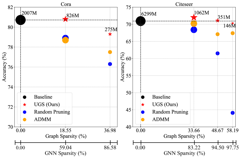
Figure 1: Summary of our achieved performance (y-axis) at different graph and GNN sparsity levels (x-axis) on Cora and Citeceer node classification. The size of markers represent the inference MACs ($=\frac{1}{2}$ FLOPs) of each sparse GCN on the corresponding sparsified graphs. Black circles ($\bullet$) indicate the baseline, i.e., unpruned dense GNNs on the full graph. Blue circles (${\color[rgb]{0,0,1}\bullet}$) are random pruning results. Orange circles (${\color[rgb]{1,.5,0}\bullet}$) represent the performance of a previous graph sparsification approach, i.e., ADMM (Li et al., 2020b). Red stars (★) are established by our method (UGS).

However, the training and inference of GNNs suffer from the notorious inefficiency, and pose hurdle to GNNs from being scaled up to real-world large-scale graph applications. This hurdle arises from both algorithm and hardware levels. On the algorithm level, GNN models can be thought of a composition of traditional graphs equipped with deep neural network (DNN) algorithms on vertex features. The execution of GNN inference falls into three distinct categories with unique computational characteristics: graph traversal, DNN computation, and aggregation. Especially, GNNs broadly follow a recursive neighborhood aggregation (or message passing) scheme, where each node aggregates feature vectors of its multi-hop neighbors to compute its new feature vector. The aggregation phase costs massive computation when the graphs are large and with dense/complicated neighbor connections (Xu et al., 2018). On the hardware level, GNN’s computational structure depends on the often sparse and irregular structure of the graph adjacency matrices. This results in many random memory accesses and limited data reuse, but also requires relatively little computation. As a result, GNNs have much higher inference latency than other neural networks, limiting them to applications where inference can be pre-computed offline (Geng et al., 2020; Yan et al., 2020).

This paper aims at aggressively trimming down the explosive GNN complexity, from the algorithm level. There are two streams of works: simplifying the graph, or simplifying the model. For the first stream, many have explored various sampling-based strategies (Hübler et al., 2008; Chakeri et al., 2016; Calandriello et al., 2018; Adhikari et al., 2017; Leskovec & Faloutsos, 2006; Voudigari et al., 2016; Eden et al., 2018; Zhao, 2015; Chen et al., 2018a), often combined with mini-batch training algorithms for locally aggregating and updating features. Zheng et al. (2020) investigated graph sparsification, i.e., pruning input graph edges, and learned an extra DNN surrogate. Li et al. (2020b) also addressed graph sparsification by formulating an optimization objective, solved by alternating direction method of multipliers (ADMM) (Bertsekas & Rheinboldt, 1982).

The second stream of efforts were traditionally scarce, since the DNN parts of most GNNs are (comparably) lightly parameterized, despite the recent emergence of increasingly deep GNNs (Li et al., 2019). Although model compression is well studied for other types of DNNs (Cheng et al., 2017), it has not been discussed much for GNNs. One latest work (Tailor et al., 2021) explored the viability of training quantized GNNs, enabling the usage of low precision integer arithmetic during inference. Other forms of well-versed DNN compression techniques, such as model pruning (Han et al., 2016), have not been exploited for GNNs up to our best knowledge. More importantly, no prior discussion was placed on jointly simplifying the input graphs and the models for GNN inference. In view of such, this paper asks: to what extent could we co-simplify the input graph and the model, for ultra-efficient GNN inference?

1.1 Summary of Our Contributions

This paper makes multi-fold contributions to answer the above questions. Unlike pruning convolutional DNNs which are heavily overparameterized, directly pruning the much less parameterized GNN model would have only limited room to gain. Our first technical innovation is to for the first time present an end-to-end optimization framework called unified GNN sparsification (UGS) that simultaneously prunes the graph adjacency matrix and the model weights. UGS makes no assumption to any GNN architecture or graph structure, and can be flexibly applied across various graph-based learning scenarios at scale.

Considering UGS as the generalized pruning for GNNs, our second technical innovation is to generalize the popular lottery ticket hypothesis (LTH) to GNNs for the first time. LTH (Frankle & Carbin, 2018) demonstrates that one can identify highly sparse and independently trainable subnetworks from dense models, by iterative pruning. It was initially observed in convolutional DNNs, and later broadly found in natural language processing (NLP) (Chen et al., 2020b), generative models (Kalibhat et al., 2020), reinforcement learning (Yu et al., 2020) and lifelong learning (Chen et al., 2020b). To meaningfully generalize LTH to GNNs, we define a graph lottery ticket (GLT) as a pair of core sub-dataset and sparse sub-network which can be jointly identified from the full graph and the original GNN model, by iteratively applying UGS. Like its counterpart in convolutional DNNs, a GLT could be trained from its initialization to match the performance of training with the full model and graph, and its inference cost is drastically smaller.

Our proposal has been experimentally verified, across various GNN architectures and diverse tasks, on both small-scale graph datasets (Cora, Citeseer and PubMed), and large-scale datasets from the challenging Open Graph Benchmark (OGB). Our main observations are outlined below:

• UGS is widely applicable to simplifying a GNN during training and reducing its inference MACs (multiply–accumulate operations). Moreover, by iteratively applying UGS, GLTs can be broadly located from for both shallow and deep GNN models, on both small- and large-scale graph datasets, with substantially reduced inference costs and unimpaired generalization.

• For node classification, our found GLTs achieve $20\%\sim 98\%$ MACs saving, with up to $5\%\sim 58.19\%$ sparsity on graphs and $20\%\sim 97.75\%$ sparsity on GNN models, at little to no performance degradation. For example in Figure 1, on Cora and Citeseer node classification, our GLTs (★) achieve comparable or sometimes even slightly better performance than the baselines of full models and graphs (${\color[rgb]{0,0,0}\bullet}$), with only $41.16\%$ and $5.57\%$ MACs, respectively.

• For link prediction, GLTs lead to $48\%\sim 97\%$ and $70\%$ MACs saving, coming from up to $22.62\%\sim 55.99\%$ sparsity on graphs and and $67.23\%\sim 97.19\%$ sparsity on GNN models, again without performance loss.

• Our proposed framework can scale up to deep GNN models (up to $28$ layers) on large graphs (e.g., Ogbn-ArXiv and Ogbn-Proteins), without bells and whistles.

• Besides from random initializations, GLTs can also be drawn from the initialization via self-supervised pre-training – an intriguing phenomenon recently just reported for NLP (Chen et al., 2020b) and computer vision models (Chen et al., 2020a). Using a latest GNN pre-training algorithm (You et al., 2020b) for initialization, GLTs can be found to achieve robust performance with even sparser graphs and GNNs.

2 Related Work

Graph Neural Networks.

There are mainly three categories of GNNs (Dwivedi et al., 2020): i) extending original convolutional neural networks to the graph regime (Scarselli et al., 2008; Bruna et al., 2013; Kipf & Welling, 2016; Hamilton et al., 2017); ii) introducing anisotropic operations on graphs such as gating and attention (Battaglia et al., 2016; Monti et al., 2017; Veličković et al., 2018), and iii) improving upon limitations of existing models (Xu et al., 2019; Morris et al., 2019; Chen et al., 2019; Murphy et al., 2019). Among this huge family, Graph Convolutional Networks (GCNs) are widely adopted, which can be categorized as spectral domain based methods (Defferrard et al., 2016; Kipf & Welling, 2016) and spatial domain bases methods (Simonovsky & Komodakis, 2017; Hamilton et al., 2017).

The computational cost and memory usage of GNNs will expeditiously increase with the graph size. The aim of graph sampling or sparsification is to extract a small sub-graph from the original large one, which can remain effective for learning tasks (Zheng et al., 2020; Hamilton et al., 2017) while reducing the cost. Previous works on sampling focus on preserving certain pre-defined graph metrics (Hübler et al., 2008), graph spectrum (Chakeri et al., 2016; Adhikari et al., 2017), or node distribution (Leskovec & Faloutsos, 2006; Voudigari et al., 2016; Eden et al., 2018). FastGCN (Chen et al., 2018a) introduced a global importance sampling method instead of locally neighbor sampling. VRGCN (Chen et al., 2018b) proposed a control variate based algorithm, but requires all intermediate vertex embeddings to be saved during training. Cluster-GCN (Chiang et al., 2019) used clustering to partition subgraphs for training, but often suffers in stability. Zheng et al. (2020); Li et al. (2020b) cast graph sparsification as optimization problems, solved by learning surrogates and ADMM, respectively.

Lottery Ticket Hypothesis (LTH).

Since the original LTH (Frankle & Carbin, 2018), a lot of works have explored the prospect of trainable sparse subnetworks in place of the full models without sacrificing performance. Frankle et al. (2019); Renda et al. (2020) introduced the rewinding techniques to scale up LTH. LTH was also adopted in different fields (Evci et al., 2019; Savarese et al., 2020; Liu et al., 2019; You et al., 2020a; Gale et al., 2019; Yu et al., 2020; Kalibhat et al., 2020; Chen et al., 2021b, 2020b, 2020c, a; Ma et al., 2021; Gan et al., 2021).

However, GNN is NOT “yet another” field that can be easily cracked by LTH. That is again due to GNNs having much smaller models, while all the aforementioned LTH works focus on simplifying their redundant models. To our best knowledge, this work is not only the first to generalize LTH to GNNs, but also the first to extend LTH from simplifying models to a new data-model co-simplification prospect.

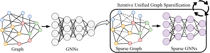
Figure 2: An illustration of unified GNN sparsification (UGS). Dash/solid lines denote the removed/remaining edges and weights in the graph and GNNs, respectively. Note that graphs and GNNs are co-optimized to find optimal solutions for the unified sparsification.

3 Methodology

3.1 Notations and Formulations

Let $\mathcal{G}=\{\mathcal{V},\mathcal{E}\}$ represent an undirected graph with $|\mathcal{V}|$ nodes and $|\mathcal{E}|$ edges. For $\mathcal{V}=\{v_{1},...,v_{|\mathcal{V}|}\}$, let $\bm{X}\in\mathbb{R}^{|\mathcal{V}|\times\mathrm{F}}$ denote the node feature matrix of the whole graph, where $\bm{x}_{i}=\bm{X}[i,:]$ is the $\mathrm{F}$-dimensional attribute vector of node $v_{i}\in\mathcal{V}$. As for $\mathcal{E}=\{e_{1},...,e_{\mathcal{|E|}}\}$, $e_{n}=(v_{i},v_{j})\in\mathcal{E}$ means that there exists a connection between node $v_{i}$ and $v_{j}$. An adjacency matrix $\bm{A}\in\mathbb{R}^{|\mathcal{V}|\times|\mathcal{V}|}$ is defined to describe the overall graph topology, where $\bm{A}[i,j]=1$ if $(v_{i},v_{j})\in\mathcal{E}$ else $\bm{A}[i,j]=0$. For example, the two-layer GNN (Kipf & Welling, 2016) can be defined as follows:

$$\bm{Z}=\mathcal{S}(\bm{\hat{A}}\sigma(\bm{\hat{A}}\bm{X}\bm{\Theta}^{(0)})\bm{\Theta}^{(1)}),$$ (1)

where $\bm{Z}$ is the prediction of GNN $f(\mathcal{G},\bm{\Theta})$. The graph $\mathcal{G}$ can be alternatively denoted as $\{\bm{A},\bm{X}\}$, $\bm{\Theta}=(\bm{\Theta}^{(0)},\bm{\Theta}^{(1)})$ is the weights of the two-layer GNN, $\mathcal{S}(\cdot)$ represents the softmax function, $\sigma(\cdot)$ denotes the activation function (e.g., ReLU), $\bm{\hat{A}}=\bm{\tilde{D}}^{-\frac{1}{2}}(\bm{A}+\bm{I})\bm{\tilde{D}}^{\frac{1}{2}}$ is normalized by the degree matrix $\bm{\tilde{D}}$ of $\bm{A}+\bm{I}$. Considering the transductive semi-supervised classification task, the objective function $\mathcal{L}$ is:

$$\mathcal{L}(\mathcal{G},\bm{\Theta})=-\frac{1}{|\mathcal{V}_{\mathrm{label}}|}\sum_{v_{i}\in\mathcal{V}_{\mathrm{label}}}\bm{y}_{i}\mathrm{log}(\bm{z}_{i}),$$ (2)

where $\mathcal{L}$ is the cross-entropy loss over all labeled samples $\mathcal{V}_{\mathrm{label}}\subset\mathcal{V}$, and $\bm{y}_{i}$ is the annotated label vector of node $v_{i}$ for its corresponding prediction $\bm{z}_{i}=\bm{Z}[i,:]$.

3.2 Unified GNN Sparsification

We present out end-to-end framework, Unified GNN Sparsification (UGS), to simultaneously reduce edges in $\mathcal{G}$ and the parameters in GNNs. Specifically, we introduce two differentiable masks $\bm{m}_{g}$ and $\bm{m}_{\theta}$ for indicating the insignificant connections and weights in the graph and GNNs, respectively. The shapes of $\bm{m}_{g}$ and $\bm{m}_{\theta}$ are identical to those the adjacency matrix $\bm{A}$ and the weights $\bm{\Theta}$, respectively. Given $\bm{A}$, $\bm{\Theta}$, $\bm{m}_{g}$ and $\bm{m}_{\theta}$ are co-optimized from end to end, under the following objective:

$$\begin{array}[]{ll}\mathcal{L}_{\mathrm{UGS}}\mathrel{\mathop{:}}=&\mathcal{L}(\{\bm{m}_{g}\odot\bm{A},\bm{X}\},\bm{m}_{\theta}\odot\bm{\Theta})\\ &+\gamma_{1}\|\bm{m}_{g}\|_{1}+\gamma_{2}\|\bm{m}_{\theta}\|_{1},\end{array}$$ (5)

where $\odot$ is the element-wise product, $\gamma_{1}$ and $\gamma_{2}$ are the hyparameters to control $\ell_{1}$ sparsity regularizers of $\bm{m}_{g}$ and $\bm{m}_{\theta}$ respectively. After the training is done, we set the lowest-magnitude elements in $\bm{m}_{g}$ and $\bm{m}_{\theta}$ to zero, w.r.t. pre-defined ratios $p_{g}$ and $p_{\theta}$. Then, the two sparse masks are applied to prune $\bm{A}$ and $\bm{\Theta}$, leading to the final sparse graph and model. Alg. 1 outlines the procedure of UGS, and it can be considered as the generalized pruning for GNNs.

Algorithm 1 Unified GNN Sparsification (UGS)

0:  Graph $\mathcal{G}=\{\bm{A},\bm{X}\}$, GNN $f(\mathcal{G},\bm{\Theta}_{0})$, GNN’s initialization $\bm{\Theta}_{0}$, initial masks $\bm{m}_{g}^{0}=\bm{A}$, $\bm{m}_{\theta}^{0}=\bm{1}\in\mathbb{R}^{\|\Theta_{0}\|_{0}}$, Step size $\eta$, $\lambda_{g}$, and $\lambda_{\theta}$.

0:  Sparsified masks $\bm{m}_{g}$ and $\bm{m}_{\theta}$

1:  for iteration $i=0,1,2,...,\mathrm{N}-1$ do

2:     Forward $f(\cdot,\bm{m}_{\theta}^{i}\odot\bm{\Theta}_{i})$ with $\mathcal{G}=\{\bm{m}_{g}^{i}\odot\bm{A},\bm{X}\}$ to compute the loss $\mathcal{L}_{\mathrm{UGS}}$ in Equation 5.

3:     Backpropagate to update $\bm{\Theta}_{i+1}\leftarrow\bm{\Theta}_{i}-\eta\nabla_{\bm{\Theta}_{i}}\mathcal{L}_{\mathrm{UGS}}$.

4:     Update $\bm{m}_{g}^{i+1}\leftarrow\bm{m}_{g}^{i}-\lambda_{g}\nabla_{\bm{m}_{g}^{i}}\mathcal{L}_{\mathrm{UGS}}$.

5:     Update $\bm{m}_{\theta}^{i+1}\leftarrow\bm{m}_{\theta}^{i}-\lambda_{\theta}\nabla_{\bm{m}_{\theta}^{i}}\mathcal{L}_{\mathrm{UGS}}$.

6:  end for

7:  Set $p_{g}=5\%$ of the lowest magnitude values in $\bm{m}_{g}^{\mathrm{N}}$ to $0$ and others to $1$, then obtain $\bm{m}_{g}$.

8:  Set $p_{\theta}=20\%$ of the lowest magnitude values in $\bm{m}_{\theta}^{\mathrm{N}}$ to $0$ and others to $1$, then obtain $\bm{m}_{\theta}$.

Algorithm 2 Iterative UGS to find Graph Lottery Tickets

0:  Graph $\mathcal{G}=\{\bm{A},\bm{X}\}$, GNN $f(\mathcal{G},\bm{\Theta}_{0})$, GNN’s initialization $\bm{\Theta}_{0}$, pre-defined sparsity levels $s_{g}$ for graphs and $s_{\theta}$ for GNNs, Initial masks $\bm{m}_{g}=\bm{A}$, $\bm{m}_{\theta}=\bm{1}\in\mathbb{R}^{\|\Theta_{0}\|_{0}}$.

0:  GLT $f(\{\bm{m}_{g}\odot\bm{A},\bm{X}\},\bm{m}_{\theta}\odot\bm{\Theta}_{0})$

1:  while $1-\frac{\|\bm{m}_{g}\|_{0}}{\|\bm{A}\|_{0}}<s_{g}$ and $1-\frac{\|\bm{m}_{\theta}\|_{0}}{\|\bm{\Theta}\|_{0}}<s_{\theta}$ do

2:     Sparsify GNN $f(\cdot,\bm{m}_{\theta}\odot\bm{\Theta}_{0})$ with $\mathcal{G}=\{\bm{m}_{g}\odot\bm{A},X\}$ using UGS, as presented in Algorithm 1.

3:     Update $\bm{m}_{g}$ and $\bm{m}_{\theta}$ accordingly.

4:     Rewinding GNN’s weights to $\bm{\Theta}_{0}$

5:     Rewinding masks, $\bm{m}_{g}=\bm{m}_{g}\odot\bm{A}$

6:  end while

3.3 Graph Lottery Tickets

Graph lottery tickets (GLT).

Given a GNN $f(\cdot,\bm{\Theta})$ and a graph $\mathcal{G}=\{\bm{A},\bm{X}\}$, the associated subnetworks of GNN and sub-graph can be defined as $f(\cdot,\bm{m}_{\theta}\odot\bm{\Theta})$ and $\mathcal{G}_{s}=\{\bm{m}_{g}\odot\bm{A},\bm{X}\}$, where $\bm{m}_{g}$ and $\bm{m}_{\theta}$ are binary masks defined in Section 3.2. If a subnetwork $f(\cdot,\bm{m}_{\theta}\odot\bm{\Theta})$ trained on a sparse graph $\mathcal{G}_{s}$ has performance matching or surpassing the original GNN trained on the full graph $\mathcal{G}$ in terms of achieved standard testing accuracy, then we define $f(\{\bm{m}_{g}\odot\bm{A},\bm{X}\},\bm{m}_{\theta}\odot\bm{\Theta}_{0})$ as a unified graph lottery tickets (GLTs), where $\bm{\Theta}_{0}$ is the original initialization for GNNs which the found lottery ticket subnetwork is usually trained from.

Unlike previous LTH literature (Frankle & Carbin, 2018), our identified GLT will consist of three elements: i) a sparse graph $\mathcal{G}_{s}=\{\bm{m}_{g}\odot\bm{A},\bm{X}\}$; ii) the sparse mask $\bm{m}_{\theta}$ for the model weight; and iii) the model weight’s initialization $\bm{\Theta_{0}}$.

Finding GLT.

Classical LTH leverages iterative magnitude-based pruning (IMP) to identify lottery tickets. In a similar fashion, we apply our UGS algorithm to prune both the model and the graph during training, as outlined Algorithm 2, obtaining the graph mask $\bm{m}_{g}$ and model weight mask $\bm{m}_{\theta}$ of GLT. Then, the GNN weights are rewound to the original initialization $\bm{\Theta}$. We repeat the above two steps iteratively, until reaching the desired sparsity $s_{g}$ and $s_{\theta}$ for the graph and GNN, respectively.

Complexity analysis of GLTs.

The inference time complexity of GLTs is $\mathcal{O}(\mathrm{L}\times\|\bm{m}_{g}\odot\bm{A}\|_{0}\times\mathrm{F}+\mathrm{L}\times\|m_{\theta}\|_{0}\times|\mathcal{V}|\times\mathrm{F}^{2})$, where $\mathrm{L}$ is the number of layers, $\|\bm{m}_{g}\odot\bm{A}\|_{0}$ is the number of remaining edges in the sparse graph, $\mathrm{F}$ is the dimension of node features, $|\mathcal{V}|$ is the number of nodes. The memory complexity is $\mathcal{O}(\mathrm{L}\times|\mathcal{V}|\times\mathrm{F}+\mathrm{L}\times\|m_{\theta}\|_{0}\times\mathrm{F}^{2})$. In our implementation, pruned edges will be removed from $\mathcal{E}$, and would not participate in the next round’s computation.

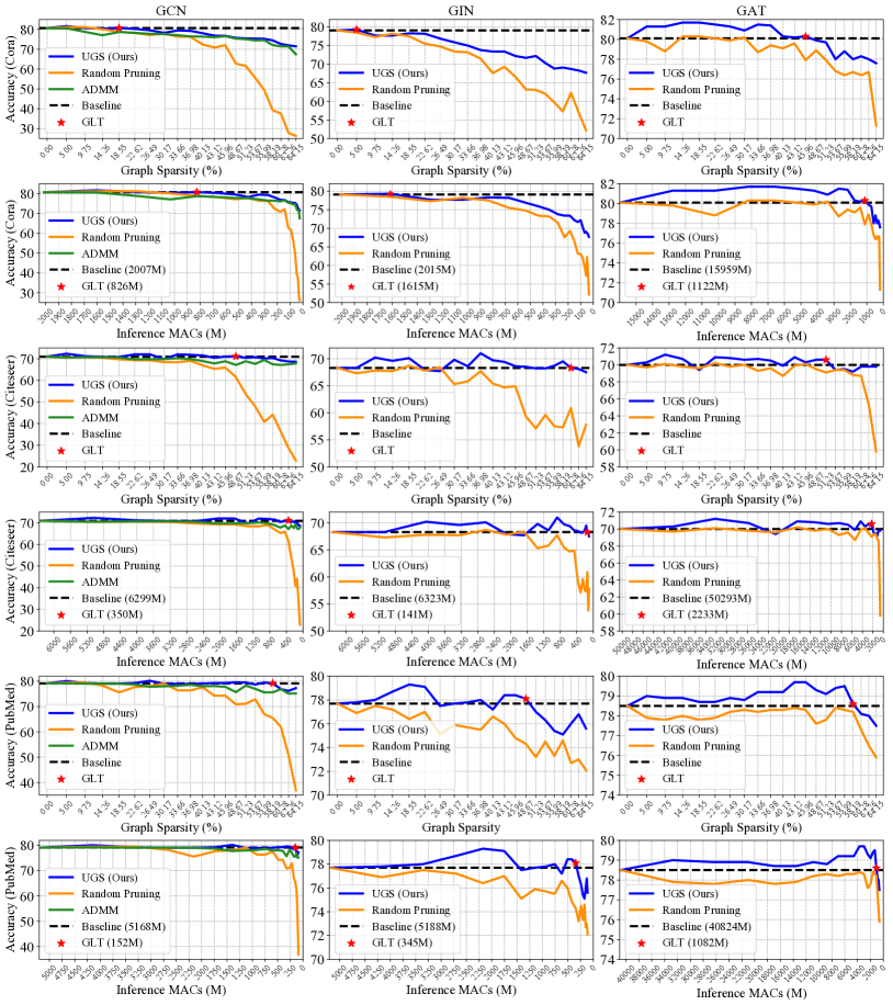
Figure 3: Node classification performance over achieved graph sparsity levels or inference MACs of GCN, GIN, and GAT on Cora, Citeseer, and PubMed datasets, respectively. Red stars (★) indicate the located GLTs, which reach comparable performance with high sparsity and low inference MACs. Dash lines represent the baseline performance of full GNNs on full graphs. More results over GNN sparsity are provided in Appendix A2.1.

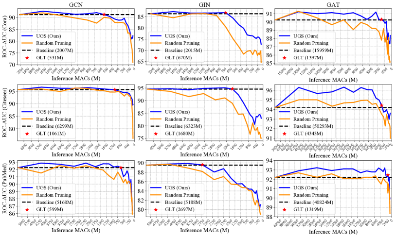
Figure 4: Link prediction performance over inference MACs of GCN, GIN, and GAT on Cora, Citeseer, and PubMed datasets, respectively. Red stars (★) indicate the located GLTs, which reach comparable performance with the least inference MACs. Dash lines represent the baseline performance of unpruned GNNs on full graphs. More results over graph sparsity and GNN sparsity are referred to Appendix A2.2.

Table 1: Graph datasets statistics.

Dataset	Task Type	Nodes	Edges	Ave. Degree	Features	Classes	Metric
Cora	Node Classification	2,708	5,429	3.88	1,433	7	Accuracy
	Link Prediction						ROC-AUC
Citeseer	Node Classification	3,327	4,732	2.84	3,703	6	Accuracy
	Link Prediction						ROC-AUC
PubMed	Node Classification	19,717	44,338	4.50	500	3	Accuracy
	Link Prediction						ROC-AUC
Ogbn-ArXiv	Node Classification	169,343	1,166,243	13.77	128	40	Accuracy
Ogbn-Proteins	Node Classification	132,534	39,561,252	597.00	8	2	ROC-AUC
Ogbl-Collab	Link Prediction	235,868	1,285,465	10.90	128	2	Hits@50

4 Experiments

In this section, extensive experiments are reported to validate the effectiveness of UGS and the existence of GLTs across diverse graphs and GNN models. Our subjects include small- and medium-scale graphs with two-layer Graph Convolutional Network (GCN) (Kipf & Welling, 2016), Graph Isomorphism Network (GIN) (Xu et al., 2018), and Graph Attention Network (GAT) (Veličković et al., 2017) in Section 4.2; as well as large-scale graphs with 28-layer deep ResGCNs (Li et al., 2020a) in Section 4.2. Besides, in Section 4.3, we investigate GLTs under the self-supervised pre-training (You et al., 2020b). Ablation studies and visualizations are provided in Section 4.4 and 4.5.

Datasets

We use popular semi-supervised graph datasets: Cora, Citeseer and PubMed (Kipf & Welling, 2016), for both node classification and link prediction tasks. For experiments on large-scale graphs, we use the Open Graph Benchmark (OGB) (Hu et al., 2020), such as Ogbn-ArXiv, Ogbn-Proteins, and Ogbl-Collab. More datasets statistics are summarized in Table 1. Other details such as the datasets’ train-val-test splits are included in Appendix A1.

Training and Inference Details

Our evaluation metrics are shown in Table 1, following Kipf & Welling (2016); Hu et al. (2020); Mavromatis & Karypis (2020). More detailed configurations such as learning rate, training iterations, and hyperparameters in UGS, are referred to Appendix A1.

4.1 The Existence of Graph Lottery Ticket

We first examine whether unified graph lottery tickets exist and can be located by UGS. Results of GCN/GIN/GAT on Cora/Citesser/PubMed for node classification and link prediction are collected in Figures 3 and 4, respectively. Note that each point in the figures denotes the achieved performance with respect to a certain graph sparsity, GNN sparsity, and inference MACs. However, due to the limited space, we only include one or two of these three sparsity indicators in the main text, and the rest can be found in Appendix A2. We list the following Observations.

Obs.1. GLTs broadly exist with substantial MACs saving.

Graph lottery tickets at a range of graph sparsity from $5\%$ to $58.19\%$ without performance deterioration, can be identified across GCN, GIN and GAT on Cora, Citeseer, and PubMed datasets for both node classification and link prediction tasks. Such GLTs significantly reduce $59\%\sim 97\%$, $20\%\sim 98\%$, $91\%\sim 97\%$ inference MACs for GCN, GIN and GAT across all datasets.

Obs.2. UGS is flexible and consistently shows superior performance.

UGS consistently surpasses random pruning by substantial performance margins across all datasets and GNNs, which validates the effectiveness of our proposal. The previous state-of-the-art method, i.e., ADMM (Li et al., 2020b), achieves a competitive performance to UGS at moderate graph sparsity levels, and performs $3\sim 4\%$ worse than UGS when graphs are heavily pruned.

Note that the ADMM approach by Li et al. (2020b) is only applicable when two conditions are met: i) graphs are stored via adjacency matrices—however, that is not practical for large graphs (Hu et al., 2020); ii) aggregating features with respect to adjacency matrices—however, recent designs of GNNs (e.g., GIN and GAT) commonly use the much more computation efficient approach of synchronous/asynchronous message passing (Gilmer et al., 2017; Busch et al., 2020). On the contrary, our proposed UGS is flexible enough and free of these limitations.

Obs.3. GNN-specific and Graph-specific analyses: GAT is more amenable to sparsified graphs; Cora is more sensitive to pruning.

As demonstrated in Figures 3 and 4, compared to GCN and GIN, GLTs in GAT can be found at higher sparsity levels; meanwhile randomly pruned graphs and GAT can still reach satisfied performance and maintain higher accuracies on severely sparsified graphs.

One possible explanation is that attention-based aggregation is capable of re-identifying important connections in pruned graphs which makes GAT be more amenable to sparsification. Compared the sparsity of located GLTs (i.e., the position of red stars (★)) across three graph datasets, we find that Cora is the most sensitive graph to pruning and PubMed is more robust to be sparsified.

4.2 Scale Up Graph Lottery Tickets

To scale up graph lottery tickets, we further conduct experiments on 28-layer deep ResGCNs (Li et al., 2020a) on large-scale datasets that have more than millions of connections, like Ogbn-ArXiv and Ogbn-Proteins for node classification, Ogbl-Collab for link prediction in Table 1. We summarize our observations and derive insights below.

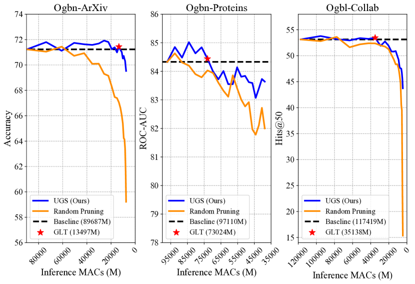
Figure 5: Node classification and link prediction performance of 28-layer deep ResGCNs on large-scale graph datasets.

Obs.4. UGS is scaleable and GLT exists in deep GCNs on large-scale datasets.

Figure 5 demonstrates that UGS can be scaled up to deep GCNs on large-scale graphs. Found GLTs obtain matched performance with $85\%$, $25\%$, $70\%$ MACs saving on Ogbn-ArXiv, Ogbn-Proteins, and Ogbl-Collab, respectively.

Obs.5. Denser graphs (e.g., Ogbn-Proteins) are more resilient to sparsification.

As shown in Figure 5, comparing the node classification results on Ogbn-ArXiv (Ave. degree: 13.77) and Ogbn-Proteins (Ave. degree: 597.00), Ogbn-Proteins has a negligible performance gap between UGS and random pruning, even on heavily pruned graphs. Since nodes with high degrees in denser graphs have less chance to be totally isolated during pruning, it may contribute to more robustness to sparsification. Similar observations can be drawn from the comparison between PubMed and other two small graphs in Figure 3 and 4.

4.3 Graph Lottery Ticket from Pre-training

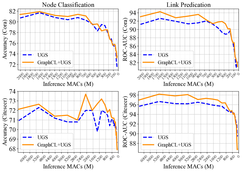
Figure 6: Drawing graph lottery tickets from randomly initialized and self-supervised pre-trained (GraphCL (You et al., 2020b)) GCNs on node classification (low label rate: only $5.0\%$ and $3.6\%$ nodes in Cora and Citesser are labeled) and link prediction.

High-quality lottery tickets can be drawn from self-supervised pre-trained models, as recently found in both NLP and computer vision fields (Chen et al., 2020b, a). In the GLT case, we also assess the impact of replacing random initialization with self-supervised graph pre-training, i.e., GraphCL (You et al., 2020b), on transductive semi-supervised node classification and link prediction.

From Figure 6 and A12, we gain a few interesting observations. First, UGS with the GraphCL pre-trained initialization consistently presents superior performance at moderate sparsity levels ($\leq 40\%$ graph sparsity $\simeq$ $\leq 85\%$ MACs saving). While the two settings perform similar at extreme sparsity, it indicates that for excessively pruned graphs, the initialization is no longer the performance bottleneck; Second, GraphCL benefits GLT on multiple downstream tasks including node classification and link prediction; Third, especially on the transductive semi-supervised setup, GLTs with appropriate sparsity levels can even enlarge the performance gain from pre-training, for example, see GLT on Citeseer with $22.62\%$ graph sparsity and $2068$M inference MACs.

4.4 Ablation Study

Pruning ratio $p_{g}$ and $p_{\theta}$.

We extensively investigate the pruning ratios $p_{g}$, $p_{\theta}$ in UGS for graph and GNN sparsification. As shown in Figure 7, with a fixed $p_{\theta}=20\%$, only the setting of $p_{g}=5\%$ can identify the GLT, and it performs close to $p_{g}=10\%$ at higher sparsity levels (e.g., $\geq 25\%$). Aggressively pruning the graph’s connections in each round of iterative UGS, e.g., $p_{g}=20\%$, leads to substantially degraded accuracies, especially for large sparsities. On the other hand, with a fixed $p_{g}=20\%$, all there settings of $p_{\theta}=10\%,20\%,40\%$ show similar performance, and even higher pruning ratios produce slight better results. It again verifies that the key bottleneck in pruning GNNs mainly lies in the sparsification of graphs. In summary, we adopt $p_{g}=5\%$ and $p_{g}=20\%$ (follow previous LTH works (Frankle & Carbin, 2018)) for all the experiments.

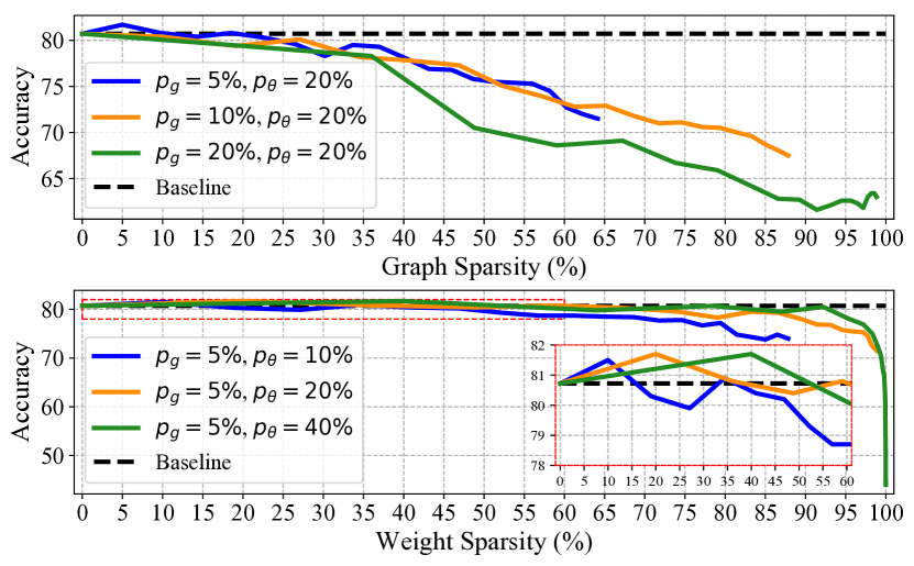
Figure 7: Ablation studies of pruning ratios for the graph and GNN sparsification by UGS, i.e., $p_{g},p_{\theta}$. Each curve records the achieved performance of $20$ rounds iterative UGS. GCN on Cora is adopted here. The embedded sub-graph is a zoom-in of the red box region.

Table 2: Performance comparisons of Random GLT versus GLT from GCN on Cora, at several sparsity levels.

Settings	(Graph Sparsity, GNN Sparsity)=$(s_{g}\%,s_{\theta}\%)$
	(18.55,59.04)	(22.62,67.23)	(36.98,86.58)	(55.99,97.19)
Random GLT	79.70	78.50	75.70	63.70
GLT	80.80	80.30	79.30	75.30

Random graph lottery tickets.

Randomly re-initializing located sparse models, i.e., random lottery tickets, usually serves as a necessary baseline for validating the effectiveness of rewinding processes (Frankle & Carbin, 2018). In Table 2, we compare GLT to Random GLT, the latter by randomly re-initializing GNN’s weights and learnable masks, and GLT shows aapparently superior performance, consistent with previous observations (Frankle & Carbin, 2018).

4.5 Visualization and Analysis

In this section, we visualize the sparsified graphs in GLTs from UGS in Figure 8, and further measure the graph properties shown in Table A5, including clustering coefficient (Luce & Perry, 1949), as well as node and edge betweenness centrality (Freeman, 1977). Specifically, clustering coefficient measures the proportion of edges between the nodes within a given node’s neighborhood; node and edge betweenness centrality show the degree of central a vertex or an edge is in the graph (Narayanan, 2005). Reported numbers in Table A5 are averaged over all the nodes.

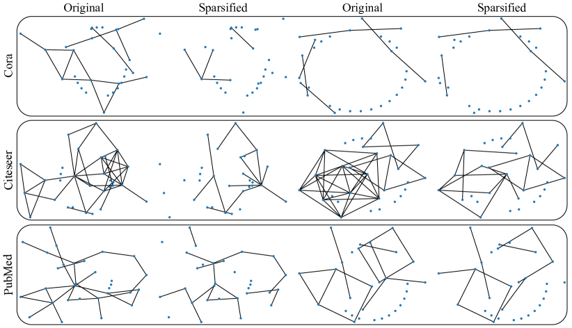
Figure 8: Visualization of sub-graphs (Original/Sparsified) from Cora, Citeseer, and PubMed. Original sub-graphs in the first and third columns are randomly sampled from full graphs. The corresponding unified sparsified sub-graphs of GLTs at $48.67\%$ sparsity, are provided in the second and forth columns.

Both Figure 8 and Table A5 show that sparse graphs obtained from UGS seem to maintain more “critical” vertices which used to have much denser connections. It may provide possible insights on what GLTs prefer to preserve.

5 Conclusion and Discussion

In this paper, we first propose unified GNN sparsification to generalize the notion or pruning in GNNs. We further establish the LTH for GNNs, by leveraging UGS and considering a novel joint data-model lottery ticekt. The new unified LTH for GNNs generalizes across various GNN architectures, learning tasks, datasets, and even initialization ways. In general, we find GLT to tremendously trim down the inference MACs, without sacrificing task performance.

It remains open how much we could translate GLT’s high sparsity into practical acceleration and energy-saving benefits. Most DNN accelerators are optimized for dense and regular computation, making edge-based operations hard to implement efficiently. To our best knowledge, the hardware acceleration research on GNNs just starts to gain interests (Auten et al., 2020; Abadal et al., 2020; Geng et al., 2020; Wang et al., 2020; Kiningham et al., 2020). We expect GLT to be implemented using sparse-dense matrix multiplication (SpMM) operations from highly optimized sparse matrix libraries, such as Intel MKL (Wang et al., 2014) or cuSPARSE (Naumov et al., 2010).

Appendix A1 More Implementation Details

Datasets Download Links.

As for small-scale datasets, we take the commonly used semi-supervised node classification graphs: Cora, Citeseer and pubMed. For larger-scale datasets, we use three Open Graph Benchmark (OGB) (Hu et al., 2020) datasets: Ogbn-ArXiv, Ogbn-Proteins and Ogbl-Collab. All the download links of adopted graph datasets are included in Table A3.

Table A3: Download links of graph datasets.

Dataset	Download links and introduction websites
Cora	https://linqs-data.soe.ucsc.edu/public/lbc/cora.tgz
Citeseer	https://linqs-data.soe.ucsc.edu/public/lbc/citeseer.tgz
PubMed	https://linqs-data.soe.ucsc.edu/public/Pubmed-Diabetes.tgz
Ogbn-ArXiv	https://ogb.stanford.edu/docs/nodeprop/#ogbn-arxiv
Ogbn-Proteins	https://ogb.stanford.edu/docs/nodeprop/#ogbn-proteins
Ogbl-Collab	https://ogb.stanford.edu/docs/linkprop/#ogbl-collab

Train-val-test Splitting of Datasets.

As for node classification of small- and medium-scale datasets, we use 140 (Cora), 120 (Citeseer) and 60 (PubMed) labeled data for training, 500 nodes for validation and 1000 nodes for testing. As for link prediction task of small- and medium-scale datasets Cora, Citeseer and PubMed, we random sample $10\%$ edges as our testing set, $5\%$ for validation, and the rest $85\%$ edges are training set. The training/validation/test splits for Ogbn-ArXiv, Ogbn-Proteins and Ogbl-Collab are given by the benchmark (Hu et al., 2020). Specifically, as for Ogbn-ArXiv, we train on the papers published until 2017, validation on those published in 2018 and test on those published since 2019. As for Ogbn-Proteins, we split the proteins nodes into training/validation/test sets according to the species which the proteins come from. As for Ogbl-Collab, we use the collaborations until 2017 as training edges, those in 2018 as validation edges, and those in 2019 as test edges.

More Details about GNNs.

As for small- and medium-scale datasets Cora, Citeseer and PubMed, we choose the two-layer GCN/GIN/GAT networks with 512 hidden units to conduct all our experiments. As for large-scale datasets Ogbn-ArXiv, Ogbn-Proteins and Ogbl-Collab, we use the ResGCN (Li et al., 2020a) with 28 GCN layers to conduct all our experiments. As for Ogbn-Proteins dataset, we also use the edge encoder module, which is a linear transform function in each GCN layer to encode the edge features. And we found if we also prune the weight of this module together with other weight, it will seriously hurt the performance, so we do not prune them in all of our experiments.

Training Details and Hyper-parameter Configuration.

We conduct numerous experiments with different hyper-parameter, such as iterations, learning rate, $\gamma_{1}$, $\gamma_{2}$, and we choose the best hyper-parameter configuration to report the final results. All the training details and hyper-parameters are summarzed in Table A4. As for Ogbn-Proteins dataset, due to its too large scale, we use the commonly used random sample method (Li et al., 2020a) to train the whole graph. Specifically, we random sample ten subgraphs from the whole graph and we only feed one subgraph to the GCN at each iteration. For each subgraph, we train 10 iterations to ensure better convergence. And we train 100 epochs for the whole graph (100 iterations for each subgraph).

Evaluation Details

We report the test accuracy/ROC-AUC/Hits@50 according to the best validation results during the training process to avoid overfitting. All training and evaluation are conducted for one run. As for the previous state-of-the-art method ADMM (Li et al., 2020b), we use the same training and evaluation setting as the original paper description, and we can reproduce the similar results compared with original paper.

Computing Infrastructures

We use the NVIDIA Tesla V100 (32GB GPU) to conduct all our experiments.

Table A4: Implementation details of node classification and link prediction.

Task	Node Classification					Link Prediction
Dataset	Cora	Citeseer	PubMed	Ogbn-ArXiv	Ogbn-Proteins	Cora	Citeseer	PubMed	Ogbn-Collab
Iteration	200	200	200	500	100	200	200	200	500
Learning Rate	8e-3	1e-2	1e-2	1e-2	1e-2	1e-3	1e-3	1e-3	1e-2
Optimizer	Admm	Admm	Admm	Admm	Admm	Admm	Admm	Admm	Admm
Weight Decay	8e-5	5e-4	5e-4	0	0	0	0	0	0
$\gamma_{1}$	1e-2	1e-2	1e-6	1e-6	1e-1	1e-4	1e-4	1e-4	1e-6
$\gamma_{2}$	1e-2	1e-2	1e-3	1e-6	1e-3	1e-4	1e-4	1e-4	1e-5

Appendix A2 More Experiment Results

A2.1 Node Classification on Small- and Medium-scale Graphs with shallow GNNs

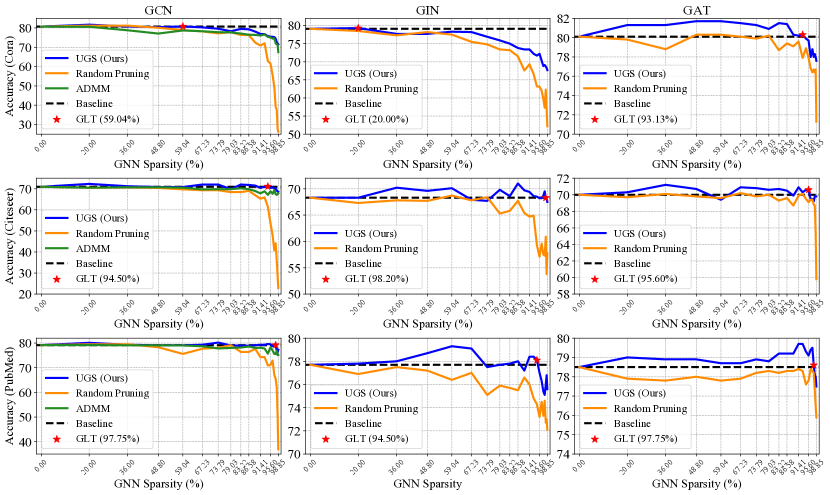
Figure A9: Node classification performance over achieved GNNs sparsity of GCN, GIN, and GAT on Cora, Citeseer, and PubMed datasets, respectively. Red stars (★) indicate the located GLTs, which reach comparable performance with extreme GNN sparsity. Dash lines represent the baseline performance of unpruned GNNs on full graphs.

As shown in Figure A9, we also provide extensive results over GNN sparsity of GCN/GIN/GAT on three small datasets, Cora/Citeseer/PubMed. We observe that UGS finds the graph wining tickets at a range of GNNs sparsity from $20\%\sim 90\%$ without performance deterioration, which significantly reduces MACs and the storage memory during both training and inference processes.

A2.2 Link Prediction on Small- and Medium-scale Graphs with shallow GNNs

More results of link prediction with GCN/GIN/GAT on Cora/Citeseer/PubMed datasets are shown in Figure A10. We observe the similar phenomenon as the node classification task: using our proposed UGS can find the graph wining tickets at a range of graph sparsity from $5\%\sim 50\%$ and GNN sparsity from $20\%\sim 90\%$ without performance deterioration, which greatly reduce the computational cost and storage space during both training and inference processes.

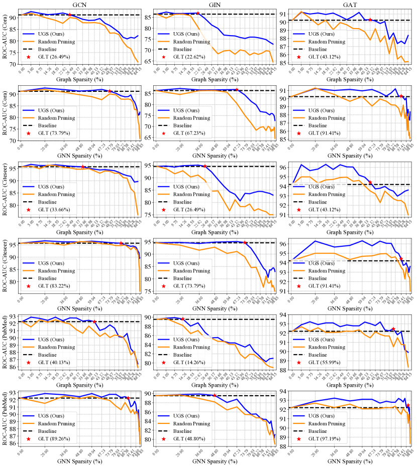
Figure A10: Link prediction performance over achieved GNNs sparsity of GCN, GIN, and GAT on Cora, Citeseer, and PubMed datasets, respectively. Red stars (★) indicate the located GLTs, which reach comparable performance with the extreme graph sparsity and GNN sparsity. Dash lines represent the baseline performance of unpruned GNNs on full graphs.

A2.3 Large-scale Graphs with Deep ResGCNs

More results of larger-scale graphs with deep ResGCNs are shown in Figure A11. Results show that our proposed UGS can found GLTs, which can reach the non-trivial sparsity levels of graph $30\%\sim 50\%$ and weight $20\%\sim 80\%$ without performance deterioration.

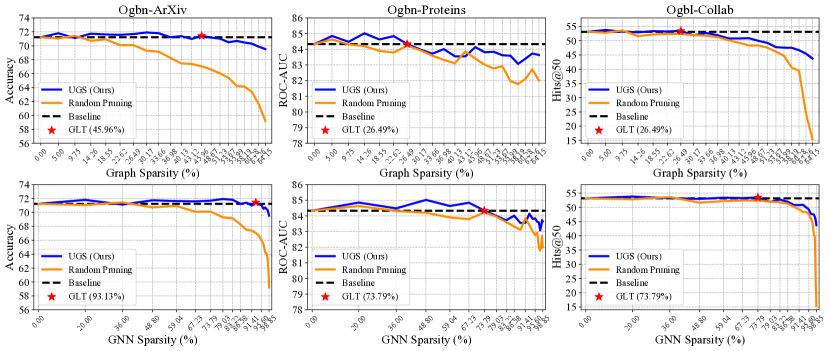
Figure A11: Node classification and link prediction performance over achieved graph sparsity and GNN sparsity of 28-layer deep ResGCNs on large-scale graph datasets.

A2.4 Graph Lottery Ticket with Pre-training

More results of node classification and link prediction on Cora and Citeseer dataset of GraphCL (You et al., 2020b) pre-training are shown in Figure A12. Results demonstrate that when using self-supervised pre-training, UGS can identify graph lottery tickets with higher qualities.

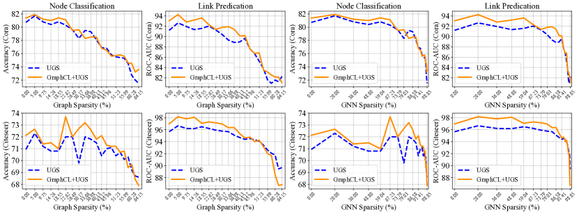
Figure A12: Drawing graph lottery tickets from randomly initialized and self-supervised pre-trained (GraphCL (You et al., 2020b)) GCNs on node classification (low label rate) and link prediction. Corresponding results over achieved graph and GNN sparsity are presented.

A2.5 More Analyses of Sparsified Graphs

As shown in Table A5, graph measurements are reported, including clustering coefficient, node and egde betweeness centrality. Results indicate that UGS seems to produce sparse graphs with more “critical” vertices which used to have more connections.

Table A5: Graph measurements of original graphs, sparse graphs from UGS, random pruning, and ADMM sparsification.

Measurements	Cora				Citeseer				PubMed
	Original	UGS	RP	ADMM	Original	UGS	RP	ADMM	Original	UGS	RP	ADMM
Clustering Coefficient	0.14147	0.07611	0.08929	0.04550	0.24067	0.15855	0.15407	0.08609	0.06018	0.03658	0.03749	0.02470
Node Betweenness	0.00102	0.00086	0.00066	0.00021	0.00165	0.00190	0.00158	0.00122	0.00027	0.00024	0.00022	0.00018
Edge Betweenness	0.00081	0.00087	0.00068	0.00032	0.00101	0.00144	0.00123	0.00137	0.00014	0.00019	0.00015	0.00018

References

- Abadal et al. (2020) Abadal, S., Jain, A., Guirado, R., López-Alonso, J., and Alarcón, E. Computing graph neural networks: A survey from algorithms to accelerators. arXiv preprint arXiv:2010.00130, 2020.
- Adhikari et al. (2017) Adhikari, B., Zhang, Y., Amiri, S. E., Bharadwaj, A., and Prakash, B. A. Propagation-based temporal network summarization. IEEE Transactions on Knowledge and Data Engineering, 30(4):729–742, 2017.
- Auten et al. (2020) Auten, A., Tomei, M., and Kumar, R. Hardware acceleration of graph neural networks. In 2020 57th ACM/IEEE Design Automation Conference (DAC), pp. 1–6. IEEE, 2020.
- Battaglia et al. (2016) Battaglia, P., Pascanu, R., Lai, M., Rezende, D. J., and kavukcuoglu, K. Interaction networks for learning about objects, relations and physics. In Proceedings of the 30th International Conference on Neural Information Processing Systems, 2016.
- Bertsekas & Rheinboldt (1982) Bertsekas, D. P. and Rheinboldt, W. Constrained optimization and lagrange multiplier methods. 1982.
- Bruna et al. (2013) Bruna, J., Zaremba, W., Szlam, A., and LeCun, Y. Spectral networks and locally connected networks on graphs. arXiv preprint arXiv:1312.6203, 2013.
- Busch et al. (2020) Busch, J., Pi, J., and Seidl, T. Pushnet: Efficient and adaptive neural message passing. arXiv preprint arXiv:2003.02228, 2020.
- Calandriello et al. (2018) Calandriello, D., Lazaric, A., Koutis, I., and Valko, M. Improved large-scale graph learning through ridge spectral sparsification. In International Conference on Machine Learning, pp. 688–697. PMLR, 2018.
- Chakeri et al. (2016) Chakeri, A., Farhidzadeh, H., and Hall, L. O. Spectral sparsification in spectral clustering. In 2016 23rd international conference on pattern recognition (icpr), pp. 2301–2306. IEEE, 2016.
- Chen et al. (2018a) Chen, J., Ma, T., and Xiao, C. Fastgcn: Fast learning with graph convolutional networks via importance sampling. In International Conference on Learning Representations, 2018a.
- Chen et al. (2018b) Chen, J., Zhu, J., and Song, L. Stochastic training of graph convolutional networks with variance reduction. In International Conference on Machine Learning, pp. 942–950. PMLR, 2018b.
- Chen et al. (2020a) Chen, T., Frankle, J., Chang, S., Liu, S., Zhang, Y., Carbin, M., and Wang, Z. The lottery tickets hypothesis for supervised and self-supervised pre-training in computer vision models. arXiv preprint arXiv:2012.06908, 2020a.
- Chen et al. (2020b) Chen, T., Frankle, J., Chang, S., Liu, S., Zhang, Y., Wang, Z., and Carbin, M. The lottery ticket hypothesis for pre-trained bert networks. arXiv preprint arXiv:2007.12223, 2020b.
- Chen et al. (2021a) Chen, T., Cheng, Y., Gan, Z., Liu, J., and Wang, Z. Ultra-data-efficient gan training: Drawing a lottery ticket first, then training it toughly. arXiv preprint arXiv:2103.00397, 2021a.
- Chen et al. (2021b) Chen, T., Zhang, Z., Liu, S., Chang, S., and Wang, Z. Long live the lottery: The existence of winning tickets in lifelong learning. In International Conference on Learning Representations, 2021b. URL https://openreview.net/forum?id=LXMSvPmsm0g.
- Chen et al. (2020c) Chen, X., Cheng, Y., Wang, S., Gan, Z., Wang, Z., and Liu, J. Earlybert: Efficient bert training via early-bird lottery tickets. arXiv preprint arXiv:2101.00063, 2020c.
- Chen et al. (2019) Chen, Z., Villar, S., Chen, L., and Bruna, J. On the equivalence between graph isomorphism testing and function approximation with gnns. In Advances in Neural Information Processing Systems, 2019.
- Cheng et al. (2017) Cheng, Y., Wang, D., Zhou, P., and Zhang, T. A survey of model compression and acceleration for deep neural networks. arXiv preprint arXiv:1710.09282, 2017.
- Chiang et al. (2019) Chiang, W.-L., Liu, X., Si, S., Li, Y., Bengio, S., and Hsieh, C.-J. Cluster-gcn: An efficient algorithm for training deep and large graph convolutional networks. In Proceedings of the 25th ACM SIGKDD International Conference on Knowledge Discovery & Data Mining, pp. 257–266, 2019.
- Defferrard et al. (2016) Defferrard, M., Bresson, X., and Vandergheynst, P. Convolutional neural networks on graphs with fast localized spectral filtering. In Proceedings of the 30th International Conference on Neural Information Processing Systems, pp. 3844–3852, 2016.
- Dwivedi et al. (2020) Dwivedi, V. P., Joshi, C. K., Laurent, T., Bengio, Y., and Bresson, X. Benchmarking graph neural networks. arXiv preprint arXiv:2003.00982, 2020.
- Eden et al. (2018) Eden, T., Jain, S., Pinar, A., Ron, D., and Seshadhri, C. Provable and practical approximations for the degree distribution using sublinear graph samples. In Proceedings of the 2018 World Wide Web Conference, pp. 449–458, 2018.
- Evci et al. (2019) Evci, U., Pedregosa, F., Gomez, A., and Elsen, E. The difficulty of training sparse neural networks. arXiv, abs/1906.10732, 2019.
- Frankle & Carbin (2018) Frankle, J. and Carbin, M. The lottery ticket hypothesis: Finding sparse, trainable neural networks. In International Conference on Learning Representations, 2018.
- Frankle et al. (2019) Frankle, J., Dziugaite, G. K., Roy, D. M., and Carbin, M. Linear mode connectivity and the lottery ticket hypothesis. arXiv, abs/1912.05671, 2019.
- Freeman (1977) Freeman, L. C. A set of measures of centrality based on betweenness. Sociometry, pp. 35–41, 1977.
- Gale et al. (2019) Gale, T., Elsen, E., and Hooker, S. The state of sparsity in deep neural networks. arXiv, abs/1902.09574, 2019.
- Gan et al. (2021) Gan, Z., Chen, Y.-C., Li, L., Chen, T., Cheng, Y., Wang, S., and Liu, J. Playing lottery tickets with vision and language. arXiv preprint arXiv:2104.11832, 2021.
- Geng et al. (2020) Geng, T., Li, A., Shi, R., Wu, C., Wang, T., Li, Y., Haghi, P., Tumeo, A., Che, S., Reinhardt, S., et al. Awb-gcn: A graph convolutional network accelerator with runtime workload rebalancing. In 2020 53rd Annual IEEE/ACM International Symposium on Microarchitecture (MICRO), pp. 922–936. IEEE, 2020.
- Gilmer et al. (2017) Gilmer, J., Schoenholz, S. S., Riley, P. F., Vinyals, O., and Dahl, G. E. Neural message passing for quantum chemistry. In International Conference on Machine Learning, pp. 1263–1272. PMLR, 2017.
- Hamilton et al. (2017) Hamilton, W., Ying, Z., and Leskovec, J. Inductive representation learning on large graphs. In Advances in neural information processing systems, pp. 1024–1034, 2017.
- Han et al. (2016) Han, S., Mao, H., and Dally, W. J. Deep compression: Compressing deep neural networks with pruning, trained quantization and huffman coding. In 4th International Conference on Learning Representations, 2016.
- Hu et al. (2020) Hu, W., Fey, M., Zitnik, M., Dong, Y., Ren, H., Liu, B., Catasta, M., and Leskovec, J. Open graph benchmark: Datasets for machine learning on graphs. arXiv preprint arXiv:2005.00687, 2020.
- Hübler et al. (2008) Hübler, C., Kriegel, H.-P., Borgwardt, K., and Ghahramani, Z. Metropolis algorithms for representative subgraph sampling. In 2008 Eighth IEEE International Conference on Data Mining, pp. 283–292. IEEE, 2008.
- Kalibhat et al. (2020) Kalibhat, N. M., Balaji, Y., and Feizi, S. Winning lottery tickets in deep generative models, 2020.
- Karimi et al. (2019) Karimi, M., Wu, D., Wang, Z., and Shen, Y. Explainable deep relational networks for predicting compound-protein affinities and contacts. arXiv preprint arXiv:1912.12553, 2019.
- Kiningham et al. (2020) Kiningham, K., Re, C., and Levis, P. Grip: A graph neural network acceleratorarchitecture. arXiv preprint arXiv:2007.13828, 2020.
- Kipf & Welling (2016) Kipf, T. N. and Welling, M. Semi-supervised classification with graph convolutional networks. arXiv preprint arXiv:1609.02907, 2016.
- Leskovec & Faloutsos (2006) Leskovec, J. and Faloutsos, C. Sampling from large graphs. In Proceedings of the 12th ACM SIGKDD international conference on Knowledge discovery and data mining, pp. 631–636, 2006.
- Li et al. (2019) Li, G., Muller, M., Thabet, A., and Ghanem, B. Deepgcns: Can gcns go as deep as cnns? In Proceedings of the IEEE/CVF International Conference on Computer Vision, pp. 9267–9276, 2019.
- Li et al. (2020a) Li, G., Xiong, C., Thabet, A., and Ghanem, B. Deepergcn: All you need to train deeper gcns. arXiv preprint arXiv:2006.07739, 2020a.
- Li et al. (2020b) Li, J., Zhang, T., Tian, H., Jin, S., Fardad, M., and Zafarani, R. Sgcn: A graph sparsifier based on graph convolutional networks. In Pacific-Asia Conference on Knowledge Discovery and Data Mining, pp. 275–287. Springer, 2020b.
- Liu et al. (2019) Liu, Z., Sun, M., Zhou, T., Huang, G., and Darrell, T. Rethinking the value of network pruning. In 7th International Conference on Learning Representations, 2019.
- Luce & Perry (1949) Luce, R. and Perry, A. D. A method of matrix analysis of group structure. Psychometrika, 14:95–116, 1949.
- Ma et al. (2021) Ma, H., Chen, T., Hu, T.-K., You, C., Xie, X., and Wang, Z. Good students play big lottery better. arXiv preprint arXiv:2101.03255, 2021.
- Mavromatis & Karypis (2020) Mavromatis, C. and Karypis, G. Graph infoclust: Leveraging cluster-level node information for unsupervised graph representation learning. arXiv preprint arXiv:2009.06946, 2020.
- Monti et al. (2017) Monti, F., Boscaini, D., Masci, J., Rodola, E., Svoboda, J., and Bronstein, M. M. Geometric deep learning on graphs and manifolds using mixture model cnns. In Proceedings of the IEEE Conference on Computer Vision and Pattern Recognition, pp. 5115–5124, 2017.
- Morris et al. (2019) Morris, C., Ritzert, M., Fey, M., Hamilton, W. L., Lenssen, J. E., Rattan, G., and Grohe, M. Weisfeiler and leman go neural: Higher-order graph neural networks. In Proceedings of the AAAI Conference on Artificial Intelligence, 2019.
- Murphy et al. (2019) Murphy, R., Srinivasan, B., Rao, V., and Ribeiro, B. Relational pooling for graph representations. In International Conference on Machine Learning, pp. 4663–4673, 2019.
- Narayanan (2005) Narayanan, S. The betweenness centrality of biological networks. PhD thesis, Virginia Tech, 2005.
- Naumov et al. (2010) Naumov, M., Chien, L., Vandermersch, P., and Kapasi, U. Cusparse library. In GPU Technology Conference, 2010.
- Qu et al. (2019) Qu, M., Bengio, Y., and Tang, J. Gmnn: Graph markov neural networks. arXiv preprint arXiv:1905.06214, 2019.
- Renda et al. (2020) Renda, A., Frankle, J., and Carbin, M. Comparing rewinding and fine-tuning in neural network pruning. In 8th International Conference on Learning Representations, 2020.
- Savarese et al. (2020) Savarese, P., Silva, H., and Maire, M. Winning the lottery with continuous sparsification. In Advances in Neural Information Processing Systems 33 pre-proceedings, 2020.
- Scarselli et al. (2008) Scarselli, F., Gori, M., Tsoi, A. C., Hagenbuchner, M., and Monfardini, G. The graph neural network model. IEEE Transactions on Neural Networks, 2008.
- Simonovsky & Komodakis (2017) Simonovsky, M. and Komodakis, N. Dynamic edge-conditioned filters in convolutional neural networks on graphs. In Proceedings of the IEEE conference on computer vision and pattern recognition, pp. 3693–3702, 2017.
- Tailor et al. (2021) Tailor, S. A., Fernandez-Marques, J., and Lane, N. D. Degree-quant: Quantization-aware training for graph neural networks. In International Conference on Learning Representations, 2021. URL https://openreview.net/forum?id=NSBrFgJAHg.
- Veličković et al. (2017) Veličković, P., Cucurull, G., Casanova, A., Romero, A., Lio, P., and Bengio, Y. Graph attention networks. arXiv preprint arXiv:1710.10903, 2017.
- Veličković et al. (2018) Veličković, P., Cucurull, G., Casanova, A., Romero, A., Liò, P., and Bengio, Y. Graph attention networks. In International Conference on Learning Representations, 2018.
- Verma et al. (2019) Verma, V., Qu, M., Lamb, A., Bengio, Y., Kannala, J., and Tang, J. Graphmix: Regularized training of graph neural networks for semi-supervised learning. arXiv preprint arXiv:1909.11715, 2019.
- Voudigari et al. (2016) Voudigari, E., Salamanos, N., Papageorgiou, T., and Yannakoudakis, E. J. Rank degree: An efficient algorithm for graph sampling. In 2016 IEEE/ACM International Conference on Advances in Social Networks Analysis and Mining (ASONAM), pp. 120–129. IEEE, 2016.
- Wang et al. (2014) Wang, E., Zhang, Q., Shen, B., Zhang, G., Lu, X., Wu, Q., and Wang, Y. Intel math kernel library. In High-Performance Computing on the Intel® Xeon Phi™, pp. 167–188. Springer, 2014.
- Wang et al. (2020) Wang, Z., Guan, Y., Sun, G., Niu, D., Wang, Y., Zheng, H., and Han, Y. Gnn-pim: A processing-in-memory architecture for graph neural networks. In Conference on Advanced Computer Architecture, pp. 73–86. Springer, 2020.
- Xu et al. (2018) Xu, K., Hu, W., Leskovec, J., and Jegelka, S. How powerful are graph neural networks? arXiv preprint arXiv:1810.00826, 2018.
- Xu et al. (2019) Xu, K., Hu, W., Leskovec, J., and Jegelka, S. How powerful are graph neural networks? In International Conference on Learning Representations, 2019. URL https://openreview.net/forum?id=ryGs6iA5Km.
- Yan et al. (2020) Yan, M., Deng, L., Hu, X., Liang, L., Feng, Y., Ye, X., Zhang, Z., Fan, D., and Xie, Y. Hygcn: A gcn accelerator with hybrid architecture. In 2020 IEEE International Symposium on High Performance Computer Architecture (HPCA), pp. 15–29. IEEE, 2020.
- Ying et al. (2018) Ying, Z., You, J., Morris, C., Ren, X., Hamilton, W., and Leskovec, J. Hierarchical graph representation learning with differentiable pooling. In Advances in Neural Information Processing Systems, pp. 4800–4810, 2018.
- You et al. (2020a) You, H., Li, C., Xu, P., Fu, Y., Wang, Y., Chen, X., Baraniuk, R. G., Wang, Z., and Lin, Y. Drawing early-bird tickets: Toward more efficient training of deep networks. In 8th International Conference on Learning Representations, 2020a.
- You et al. (2020b) You, Y., Chen, T., Sui, Y., Chen, T., Wang, Z., and Shen, Y. Graph contrastive learning with augmentations. Advances in Neural Information Processing Systems, 33, 2020b.
- You et al. (2020c) You, Y., Chen, T., Wang, Z., and Shen, Y. When does self-supervision help graph convolutional networks? In III, H. D. and Singh, A. (eds.), Proceedings of the 37th International Conference on Machine Learning, volume 119 of Proceedings of Machine Learning Research, pp. 10871–10880. PMLR, 13–18 Jul 2020c. URL http://proceedings.mlr.press/v119/you20a.html.
- You et al. (2020d) You, Y., Chen, T., Wang, Z., and Shen, Y. L2-gcn: Layer-wise and learned efficient training of graph convolutional networks. In Proceedings of the IEEE/CVF Conference on Computer Vision and Pattern Recognition, pp. 2127–2135, 2020d.
- Yu et al. (2020) Yu, H., Edunov, S., Tian, Y., and Morcos, A. S. Playing the lottery with rewards and multiple languages: lottery tickets in rl and nlp. In 8th International Conference on Learning Representations, 2020.
- Zhang & Chen (2018) Zhang, M. and Chen, Y. Link prediction based on graph neural networks. In Advances in Neural Information Processing Systems, pp. 5165–5175, 2018.
- Zhao (2015) Zhao, P. gsparsify: Graph motif based sparsification for graph clustering. In Proceedings of the 24th ACM International on Conference on Information and Knowledge Management, pp. 373–382, 2015.
- Zheng et al. (2020) Zheng, C., Zong, B., Cheng, W., Song, D., Ni, J., Yu, W., Chen, H., and Wang, W. Robust graph representation learning via neural sparsification. In International Conference on Machine Learning, 2020.
- Zhou et al. (2018) Zhou, J., Cui, G., Zhang, Z., Yang, C., Liu, Z., Wang, L., Li, C., and Sun, M. Graph neural networks: A review of methods and applications. arXiv preprint arXiv:1812.08434, 2018.