Q-Value Weighted Regression: Reinforcement Learning with Limited Data

Abstract

Sample efficiency and performance in the offline setting have emerged as significant challenges of deep reinforcement learning. We introduce Q-Value Weighted Regression (QWR), a simple RL algorithm that excels in these aspects. QWR is an extension of Advantage Weighted Regression (AWR), an off-policy actor-critic algorithm that performs very well on continuous control tasks, also in the offline setting, but has low sample efficiency and struggles with high-dimensional observation spaces. We perform an analysis of AWR that explains its shortcomings and use these insights to motivate QWR. We show experimentally that QWR matches the state-of-the-art algorithms both on tasks with continuous and discrete actions. In particular, QWR yields results on par with SAC on the MuJoCo suite and – with the same set of hyperparameters – yields results on par with a highly tuned Rainbow implementation on a set of Atari games. We also verify that QWR performs well in the offline RL setting.

1 Introduction

Deep reinforcement learning has been applied to a large number of challenging tasks, from games (Silver et al., 2017; OpenAI, 2018; Vinyals et al., 2017) to robotic control (Sadeghi & Levine, 2016; OpenAI et al., 2018; Rusu et al., 2016). Since RL makes minimal assumptions on the underlying task, it holds the promise of automating a wide range of applications. However, its widespread adoption has been hampered by a number of challenges. Reinforcement learning algorithms can be substantially more complex to implement and tune than standard supervised learning methods and can have a fair number of hyper-parameters and be brittle with respect to their choices, and may require a large number of interactions with the environment.

These issues are well-known and there has been significant progress in addressing them. The policy gradient algorithm REINFORCE (Williams, 1992) is simple to understand and implement, but is both brittle and requires on-policy data. Proximal Policy Optimization (PPO, Schulman et al. (2017)) is a more stable on-policy algorithm that has seen a number of successful applications despite requiring a large number of interactions with the environment. Soft Actor-Critic (SAC, Haarnoja et al. (2018)) is a much more sample-efficient off-policy algorithm, but it is defined only for continuous action spaces and does not work well in the offline setting, known as batch reinforcement learning, where all samples are provided from earlier interactions with the environment, and the agent cannot collect more samples. Advantage Weighted Regression (AWR, Peng et al. (2019)) is a recent off-policy actor-critic algorithm that works well in the offline setting and is built using only simple and convergent maximum likelihood loss functions, making it easier to tune and debug. It is competitive with SAC given enough time to train, but is less sample-efficient and has not been demonstrated to succeed in settings with discrete actions.

We replace the value function critic of AWR with a Q-value function. Next, we add action sampling to the actor training loop. Finally, we introduce a custom backup to the Q-value training. The resulting algorithm, which we call Q-Value Weighted Regression (QWR) inherits the advantages of AWR but is more sample-efficient and works well with discrete actions and in visual domains, e.g., on Atari games.

To better understand QWR we perform a number of ablations, checking different number of samples in actor training, different advantage estimators, and aggregation functions. These choices affect the performance of QWR only to a limited extent and it remains stable with each of the choices across the tasks we experiment with.

We run experiments with QWR on the MuJoCo environments and on a subset of the Arcade Learning Environment. Since sample efficiency is our main concern, we focus on the difficult case when the number of interactions with the environment is limited – in most our experiments we limit it to 100K interactions. The experiments demonstrate that QWR is indeed more sample-efficient than AWR. On MuJoCo, it performs on par with Soft Actor-Critic (SAC), the current state-of-the-art algorithm for continuous domains. On Atari, QWR performs on par with OTRainbow, a variant of Rainbow highly tuned for sample efficiency. Notably, we use the same set of hyperparameters (except for the network architecture) for both MuJoCo and Atari experiments. We verify that QWR performs well also in the regime where more data is available: with 1M interactions, QWR still out-perform SAC on MuJoCo on all environments we tested except for HalfCheetah.

2 Q-Value Weighted Regression

2.1 Advantage Weighted Regression

Peng et al. (2019) recently proposed Advantage Weighted Regression (AWR), an off-policy, actor-critic algorithm notable for its simplicity and stability, achieving competitive results across a range of continuous control tasks. It can be expressed as interleaving data collection and two regression tasks performed on the replay buffer, as shown in Algorithm 1.

1:  $\theta\leftarrow$ random actor parameters

2:  $\phi\leftarrow$ random critic parameters

3:  $\mathcal{D}\leftarrow\emptyset$

4:  for $k$ in $0..n\_iterations-1$ do

5:     add trajectories $\{\tau_{i}\}$ sampled by $\pi_{\theta}$ to $\mathcal{D}$

6:     for $i$ in $0..n\_critic\_steps-1$ do

7:        sample $(\mathbf{s,a})\sim\mathcal{D}$

8:        $\phi\leftarrow\phi-\alpha_{V}\nabla_{\phi}||\mathcal{R}_{\mathcal{D}}^{\mathbf{s,a}}-V_{\phi}(\mathbf{s})||^{2}$

9:     end for

10:     for $i$ in $0..n\_actor\_steps-1$ do

11:        sample $(\mathbf{s,a})\sim\mathcal{D}$

12:        $\xi\leftarrow\exp(\frac{1}{\beta}(\mathcal{R}_{\mathcal{D}}^{\mathbf{s,a}}-V_{\phi}(\mathbf{s}))$

13:        $\theta\leftarrow\theta+\alpha_{\pi}\nabla_{\theta}\log\pi_{\theta}(\mathbf{a|s})~{}\xi$

14:     end for

15:  end for

Algorithm 1 Advantage Weighted Regression.

AWR optimizes expected improvement of an actor policy $\pi(\mathbf{a}|\mathbf{s})$ over a sampling policy $\mu(\mathbf{a}|\mathbf{s})$ by regression towards the well-performing actions in the collected experience. Improvement is achieved by weighting the actor loss by exponentiated advantage $A_{\mu}(\mathbf{s,a})$ of an action, skewing the regression towards the better-performing actions. The advantage is calculated based on the expected return $\mathcal{R}_{\mu}^{\mathbf{s,a}}$ achieved by performing action $\mathbf{a}$ in state $\mathbf{s}$ and then following the sampling policy $\mu$. To calculate the advantage, one first estimates the value, $V_{\mu}(s)$, using a learned critic and then computes $A_{\mu}(\mathbf{s,a})=\mathcal{R}_{\mu}^{\mathbf{s,a}}-V_{\mu}(\mathbf{s})$. This results in the following formula for the actor:

$$\begin{split}\mathrm{argmax}_{\pi}\mathbb{E}_{\mathbf{s}\sim d_{\mu}}\mathbb{E}_{\mathbf{a}\sim\mu(\cdot|\mathbf{s})}\log\pi(\mathbf{a}|\mathbf{s})~{}\xi^{\mathbf{s,a}}_{\mu},&\\ \textrm{where}~{}\xi^{\mathbf{s,a}}_{\mu}=\exp\left(\frac{1}{\beta}(\mathcal{R}_{\mu}^{\mathbf{s,a}}-V_{\mu}(\mathbf{s}))\right).&\end{split}$$ (1)

In this formula $d_{\mu}(\mathbf{s})=\sum_{t=1}^{\infty}\gamma^{t-1}p(\mathbf{s}_{t}=\mathbf{s}|\mu)$ denotes the unnormalized, discounted state visitation distribution of the policy $\mu$, and $\beta$ is a temperature hyperparameter.

The critic is trained to estimate the future returns of the sampling policy $\mu$:

$$\mathrm{argmin}_{V}\mathbb{E}_{\mathbf{s}\sim d_{\mu}(\mathbf{s})}\mathbb{E}_{\mathbf{a}\sim\mu(\cdot|\mathbf{s})}\left[||\mathcal{R}_{\mu}^{\mathbf{s,a}}-V(\mathbf{s})||^{2}\right].$$ (2)

To achieve off-policy learning, the actor and the critic are trained on data collected from a mixture of policies from different training iterations, stored in the replay buffer $\mathcal{D}$.

2.2 Analysis of AWR with Limited Data

While AWR achieves very good results after longer training, it is not very sample efficient, as noted in the future work section of Peng et al. (2019). To understand this problem, we analyze a single loop of actor training in AWR under a special assumption.

The assumption we introduce, called state-determines-action, concerns the content of the replay buffer $\mathcal{D}$ of an off-policy RL algorithm. The replay buffer contains the state-action pairs that the algorithm has visited so far during its interactions with the environment. We say that a replay buffer $\mathcal{D}$ satisfies the state-determines-action assumption when for each state $s$ in the buffer, there is a unique action that was taken from it, formally:

$$\text{for all }(s,a),(s^{\prime},a^{\prime})\in\mathcal{D}:s=s^{\prime}\implies a=a^{\prime}.$$

This assumption may seem limiting and indeed – it is not true in many of the artificial experiments with RL algorithms, with discrete state and action spaces. In such settings, even a random policy starting from the same state could violate the assumption the second time it collects a trajectory. But note that state-determines-action is almost always satisfied in continuous control, where even a slightly random policy is unlikely to ever perform the exact same action twice and transition to exactly the same state.

Note that our assumption applies well to real-world experiments with high-dimensional state spaces, as any amount of noise added to a high-dimensional space will make repeating the exact same state highly improbable. For example, consider a robot observing 32x32 pixel images. To repeat an observation, each of the 1024 pixels would have to have exactly the same value, which is close to impossible, even with a small amount of pixel noise coming from a camera. This assumption also holds in cases with limited data, even in discrete state and action spaces. When the number of collected trajectories is not enough to span the state space, it is unlikely a state will be repeated in the replay buffer. This makes our assumption particularly relevant to the study of sample efficiency.

We emphasize that the state-determines-action assumption, by design, considers exact equality of states. Two very similar, but not equal states that lead to different actions do not violate our assumption. This makes it irrelevant to reinforcement learning with linear functions as linear functions cannot separate similar states. However, it is relevant in deep RL because deep neural networks can indeed distinguish even very similar inputs (Szegedy et al., 2014; Bartlett et al., 2017; Zhang et al., 2016).

How does AWR perform under the state-determines-action assumption? In Theorems 1 and 2 (see Appendix 6.2 for more details), we show that for popular choices of discrete and Gaussian distributions the AWR update rule under this assumption will converge to a policy that assigns probability 1 to the actions already present in the replay buffer, thus cloning the previous behaviors. This is not the desired behavior, as an agent should consider various actions from each state, to ensure exploration.

Theorem 1.

Let $\mathcal{A}$ be a discrete action space. Let a replay buffer $\mathcal{D}\subseteq\mathcal{S}\times\mathcal{A}$ satisfy the state-determines-action assumption. Let $\pi_{\mathcal{D}}$ be the probability function of a distribution that clones the behavior from $\mathcal{D}$, i.e., that assigns to each state $s$ from $\mathcal{D}$ the action $a$ such that $(s,a)\in\mathcal{D}$ with probability $1$. Then, under the AWR update, $\pi^{i+1}_{\mathcal{D}}\leftarrow\pi_{\mathcal{D}}$.

The state-determines-action assumption is the main motivating point behind QWR, whose theoretical properties are proven in Theorem 3 in Appendix 6.3. We now illustrate the importance of this assumption by creating a simple environment in which it holds with high probability. We verify experimentally that AWR fails on this simple environment, while QWR is capable of solving it.

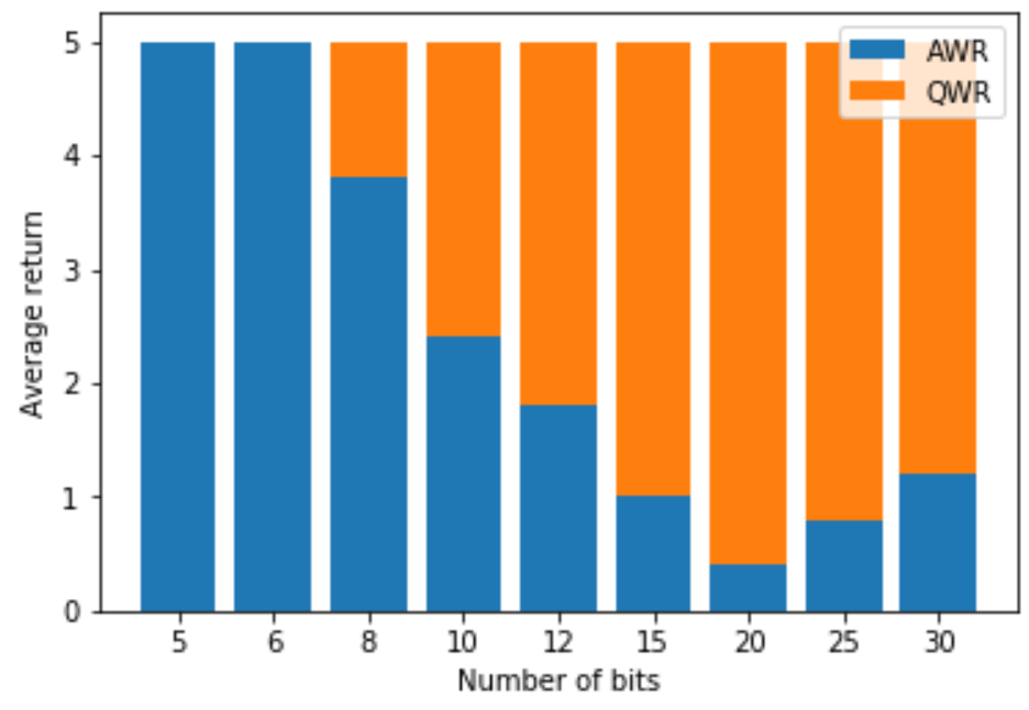
Figure 1: AWR and QWR on the BitFlip environment. The maximum possible return is 5.

The environment, which we call BitFlip, is parameterized by an integer $N$. The state of the environment consists of $N$ bits and a step counter. The action space consists of $N$ actions. When an action $i$ is chosen, the $i$-th bit is flipped and the step counter is incremented. A game of BitFlip starts in a random state with the step counter set to 0, and proceeds for 5 steps. The initial state is randomized in such a way to always leave at least 5 bits set to 0. At each step, the reward is $+1$ if a bit was flipped from $0$ to $1$ and the reward is $-1$ in the opposite case.

Since BitFlip starts in one random state out of $2^{N}$, at large enough $N$ it is highly unlikely that the starting state will ever be repeated in the replay buffer. As the initial policy is random and BitFlip maintains a step counter to prevent returning to a state, the same holds for subsequent states.

BitFlip is a simple game with a very simple strategy, but the initial replay buffer will satisfy the state-determines-action assumption with high probability. As we will see, this is enough to break AWR. We ran both AWR and QWR on BitFlip for different values of $N$, for 10 iterations per experiment. In each iteration we collected 1000 interactions with the environment and trained both the actor and the critic for 300 steps. All shared hyperparameters of AWR and QWR were set to the same values, and the backup operator in QWR was set to mean. We report the mean out of 10 episodes played by the trained agent. The results are shown in Figure 1.

As we can see, the performance of AWR starts deteriorating at a relatively small value of $N~{}=~{}8$, which corresponds to a state space with $5\cdot 2^{8}=1280$ states, while QWR maintains high performance even at $N=30$, so around $5\cdot 10^{9}$ states. Notice how the returns of AWR drop with $N$ – at higher values: $20-30$, the agent struggles to flip even a single zero bit. This problem with AWR and large state spaces motivates us to introduce QWR next.

2.3 Q-Value Weighted Regression

1:  $\theta\leftarrow$ random actor parameters

2:  $\phi\leftarrow$ random critic parameters

3:  $\mathcal{D}\leftarrow\emptyset$

4:  for $k$ in $0..n\_iterations-1$ do

5:     add trajectories $\{\tau_{i}\}$ sampled by $\pi_{\theta}$ to $\mathcal{D}$

6:     $\phi_{t}\leftarrow\phi$

7:     for $i$ in $0..n\_critic\_steps-1$ do

8:        if $i\mod update\_frequency=0$ then

9:           $\phi_{t}\leftarrow\phi$

10:        end if

11:        sample $(\mathbf{s},\mathbf{\mu},\mathbf{a,r,s^{\prime}})\sim\mathcal{D}$

12:        sample $\mathbf{a^{\prime}}_{0},...,\mathbf{a^{\prime}}_{n-1}\sim\mathbf{\mu}(\cdot|\mathbf{s^{\prime}})$

13:        $Q^{\star}\leftarrow\mathbf{r}+\gamma F(\{Q_{\phi_{t}}(\mathbf{s^{\prime},a^{\prime}}_{j})~{}|~{}j\in\{0,...,n-1\}\})$

14:        $\phi\leftarrow\phi-\alpha_{V}\nabla_{\phi}||Q^{\star}-Q_{\phi}(\mathbf{s,a})||^{2}$

15:     end for

16:     for $i$ in $0..n\_actor\_steps-1$ do

17:        sample $(\mathbf{s},\mu,...)\sim\mathcal{D}$

18:        sample $\mathbf{a}_{0},...,\mathbf{a}_{n-1}\sim\mu(\cdot|\mathbf{s})$

19:        $\hat{V}\leftarrow\frac{1}{n}\sum_{j=0}^{n-1}Q_{\phi}(\mathbf{s,a}_{j})$

20:        $\xi\leftarrow\exp(\frac{1}{\beta}(Q_{\phi}(\mathbf{s,a}_{j})-\hat{V}))$

21:        $\theta\leftarrow\theta+\alpha_{\pi}\nabla_{\theta}\frac{1}{n}\sum_{j=0}^{n-1}\log\pi_{\theta}(\mathbf{a}_{j}|\mathbf{s})~{}\xi$

22:     end for

23:  end for

Algorithm 2 Q-Value Weighted Regression.

To remedy the issue indicated by Theorems 1 and 2, we introduce a mechanism to consider multiple different actions that can be taken from a single state. We calculate the advantage of the sampling policy $\mu$ based on a learned Q-function: $A_{\mu}(\mathbf{s,a})=Q_{\mu}(\mathbf{s,a})-\hat{V}_{\mu}(\mathbf{s})$, where $\hat{V}_{\mu}(\mathbf{s})$ is the expected return of the policy $\mu$, expressed using $Q_{\mu}$ by expectation over actions: $\hat{V}_{\mu}(\mathbf{s})~{}=~{}\mathbb{E}_{a\sim\mu(\cdot|\mathbf{s})}Q_{\mu}(\mathbf{s,a})$. We substitute our advantage estimator into the AWR actor formula (Equation 1) to obtain the QWR actor:

$$\begin{split}\mathrm{argmax}_{\pi}\mathbb{E}_{s\sim d_{\mu}(\mathbf{s})}\mathbb{E}_{\mathbf{a}\sim\mu(\cdot|\mathbf{s})}\log\pi(\mathbf{a}|\mathbf{s})~{}\xi_{\mu}^{\mathbf{s,a}},&\\ \textrm{where}~{}\xi_{\mu}^{\mathbf{s,a}}=\exp\left(\frac{1}{\beta}(Q_{\mu}(\mathbf{s,a})-\hat{V}_{\mu}(\mathbf{s}))\right).&\end{split}$$ (3)

Similar to AWR, we implement the expectation over states in LABEL:eq:qwr_actor_loss by sampling from the replay buffer. However, to estimate the expectation over actions, we average over multiple actions sampled from $\mu$ during training. Because the replay buffer contains data from multiple different sampling policies, we store the parameters of the sampling policy $\mu(\mathbf{a}|\mathbf{s})$ conditioned on the current state in the replay buffer and restore it in each training step to compute the loss. This allows us to consider multiple different possible actions for a single state when training the actor, not only the one performed in the collected experience.

The use of a Q-network as a critic provides us with an additional benefit. Instead of regressing it towards the returns of our sampling policy $\mu$, we can train it to estimate the returns of an improved policy $\mu^{\star}$, in a manner similar to Q-learning. This allows us to optimize expected improvement over $\mu^{\star}$, providing a better baseline - as long as $\mathbb{E}_{\mathbf{a}\sim\mu^{\star}(\cdot|\mathbf{s})}Q_{\mu}(\mathbf{s},\mathbf{a})\geq\mathbb{E}_{\mathbf{a}\sim\mu(\cdot|\mathbf{s})}Q_{\mu}(\mathbf{s,a})$, the policy improvement theorem for stochastic policies (Sutton & Barto, 2018, Section 4.2) implies that the policy $\mu^{\star}$ achieves higher returns than the sampling policy $\mu$:

$$\mathbb{E}_{\mathbf{a}\sim\mu^{\star}(\cdot|\mathbf{s})}Q_{\mu}(\mathbf{s,a})\geq V_{\mu}(\mathbf{s})\Rightarrow V_{\mu^{\star}}(\mathbf{s})\geq V_{\mu}(\mathbf{s})$$ (4)

$\mu^{\star}$ need not be parametric - in fact, it is not materialized in any way over the course of the algorithm. The only requirement is that we can estimate the Q backup $\mathbb{E}_{\mathbf{a}\sim\mu^{\star}(\cdot|\mathbf{s})}Q(\mathbf{s,a})$. This allows great flexibility in choosing the form of $\mu^{\star}$. Since we want our method to work also in continuous action spaces, we cannot compute the backup exactly. Instead, we estimate it based on several samples from the sampling policy $\mu$. Our backup has the form $\mathbb{E}_{\mathbf{a}_{1},...,\mathbf{a}_{k}\sim\mu(\cdot|\mathbf{s})}F(\{Q(\mathbf{s,a}_{1}),...,Q(\mathbf{s,a}_{k})\})$. In this work, we extend the term Q-learning to mean training a Q-value using such a generalized backup. To make training of the Q-network more efficient, we use multi-step targets, described in detail in Appendix 6.4. The critic optimization objective using single-step targets is:

$$\begin{split}\mathrm{argmin}_{Q}~{}&\mathbb{E}_{\mathbf{s}\sim d_{\mu}(\mathbf{s})}\mathbb{E}_{\mathbf{a}\sim\mu(\mathbf{a}|\mathbf{s})}\mathbb{E}_{\mathbf{s^{\prime}}\sim\mathcal{T}(\cdot|\mathbf{s,a})}\\ &\mathbb{E}_{\mathbf{a^{\prime}}_{1},...,\mathbf{a^{\prime}}_{k}\sim\mu(\cdot|\mathbf{s^{\prime}})}||Q^{\star}-Q(\mathbf{s,a})||^{2},\end{split}$$ (5)

where

$$Q^{\star}=r(\mathbf{s,a})+\gamma F(\{Q_{\mu}(\mathbf{s^{\prime},a^{\prime}}_{1}),...,Q_{\mu}(\mathbf{s^{\prime},a^{\prime}}_{k})\})$$

and $\mathcal{T}(\mathbf{s^{\prime}}|\mathbf{s,a})$ is the environment’s transition distribution.

In this work, we investigate three choices of $F$: average, yielding $\mu^{\star}=\mu$; max, where $\mu^{\star}$ approximates the greedy policy; and log-sum-exp, $F(X)=\tau\log\left[\frac{1}{|X|}\sum_{x\in X}\exp(x/\tau)\right]$, interpolating between average and max with the temperature parameter $\tau$. This leads to three versions of the QWR algorithm: QWR-AVG, QWR-MAX, and QWR-LSE. The last operator, log-sum-exp, is similar to the backup operator used in maximum-entropy reinforcement learning (see e.g. Haarnoja et al. (2018)) and can be thought of as a soft-greedy backup, rewarding both high returns and uncertainty of the policy. It is our default choice and the final algorithm is shown in Algorithm 2.

3 Related work

Reinforcement learning algorithms.

Recent years have seen great advances in the field of reinforcement learning due to the use of deep neural networks as function approximators. Mnih et al. (2013b) introduced DQN, an off-policy algorithm learning a parametrized Q-value function through updates based on the Bellman equation. The DQN algorithm only computes the Q-value function, it does not learn an explicit policy. In contrast, policy-based methods such as REINFORCE (Williams, 1992) learn a parameterized policy, typically by following the policy gradient (Sutton et al., 1999) estimated through Monte Carlo approximation of future returns. Such methods suffer from high variance, causing low sample efficiency. Actor-critic algorithms, such as A2C and A3C (Sutton et al., 2000; Mnih et al., 2016), decrease the variance of the estimate by jointly learning policy and value functions, and using the latter as an action-independent baseline for calculation of the policy gradient. The PPO algorithm (Schulman et al., 2017) optimizes a clipped surrogate objective in order to allow multiple updates using the same sampled data.

Continuous control.

Lillicrap et al. (2015) adapted Q-learning to continuous action spaces. In addition to a Q-value function, they learn a deterministic policy function optimized by backpropagating the gradient through the Q-value function. Haarnoja et al. (2018) introduce Soft Actor-Critic (SAC): a method learning in a similar way, but with a stochastic policy optimizing the Maximum Entropy RL (Levine, 2018) objective. Similarly to our method, SAC also samples from the policy during training.

Advantage-weighted regression.

The QWR algorithm is a successor of AWR proposed by Peng et al. (2019), which in turn is based on Reward-Weighted Regression (RWR, Peters & Schaal (2007)) and AC-REPS proposed by Wirth et al. (2016). Mathematical and algorithmical foundations of advantage-weighted regression were developed by Neumann & Peters (2009). The algorithms share the same good theoretical properties: RWR, AC-REPS, AWR, and QWR losses can be mathematically reformulated in terms of KL-divergence with respect to the optimal policy (see formulas (7)-(10) in Peng et al. (2019)). QWR is different from AWR in the following key aspects: instead of empirical returns in the advantage estimation we train a $Q$ function (see formulas 1 and LABEL:eq:qwr_actor_loss below for precise definition) and use sampling for the actor. QWR is different from AC-REPS as it uses deep learning for function approximation and Q-learning for fitting the critic, see Section 2.

Several recent works have developed algorithms similar to QWR. We provide a brief overview and ways of obtaining them from the QWR pseudocode (Algorithm 2). AWR can be recovered by learning a value function $V(s)$ as a critic (line 14) and sampling actions from the replay buffer (lines 12 and 18 in Algorithm 2). AWAC (Nair et al., 2020) modifies AWR by learning a Q-function for the critic. We get it from QWR by sampling actions from the replay buffer (lines 12 and 18). Note that compared to AWAC, by sampling multiple actions for each state, QWR is able to take advantage of Q-learning to improve the critic. CRR (Wang et al., 2020) augments AWAC with training a distributional Q-function in line 14 and substituting different functions for computing advantage weights in line 21 . Again, compared to CRR, QWR samples multiple actions for each state, and so can take advantage of Q-learning. In a way similar to QWR, MPO (Abdolmaleki et al., 2018) samples actions during actor training to improve generalization. Compared to QWR, it introduces a dual function for dynamically tuning $\beta$ in line 21, adds a prior regularization for policy training and trains the critic using Retrace (Munos et al., 2016) targets in line 13. QWR can be thought of as a significant simplification of MPO, with addition of Q-learning to provide a better baseline for the actor. Additionally, the classical DQN (Mnih et al., 2013a) algorithm for discrete action spaces can be recovered from QWR by removing the actor training loop (lines 16-22), computing a maximum over all actions in Q-network training (line 13) and using an epsilon-greedy policy w.r.t. the Q-network for data collection.

Offline reinforcement learning.

Offline RL is the main topic of the survey Levine et al. (2020). The authors state that “offline reinforcement learning methods equipped with powerful function approximation may enable data to be turned into generalizable and powerful decision making engines”. We see this as one of the major challenges of modern RL and this work contributes to this challenge. Many current algorithms perform to some degree in offline RL, e.g., variants of DDPG and DQN developed by Fujimoto et al. (2018); Agarwal et al. (2019), as well as the MPO algorithm by Abdolmaleki et al. (2018) are promising alternatives to AWR and QWR analyzed in this work.

ABM (Siegel et al., 2020) is a method of extending RL algorithms based on policy networks to offline settings. It first learns a prior policy network on the offline dataset using a loss similar to Equation 1, and then learns the final policy network using any algorithm, adding an auxiliary term penalizing KL-divergence from the prior policy. CQL (Kumar et al., 2020) is a method of extending RL algorithms based on Q-networks to offline settings by introducing an auxiliary loss. To compute the loss, CQL samples actions on-line during training of the Q-network, similar to line 14 in QWR. EMaQ (Ghasemipour et al., 2020) learns an ensemble of Q-functions using an Expected-Max backup operator and uses it during evaluation to pick the best action. The Q-network training part is similar to QWR with $F=\max$ in line 13 in Algorithm 2.

The imitation learning algorithm MARWIL by Wang et al. (2018) confirms that the advantage-weighted regression performs well in the context of complex games.

Algorithm	Half-Cheetah	Walker	Hopper	Humanoid
QWR-LSE	$2323\pm 332$	$\mathbf{1301\pm 445}$	$\mathbf{1758\pm 735}$	$511\pm 57$
QWR-MAX	$2250\pm 254$	$1019\pm 1185$	$1187\pm 345$	$503\pm 49$
QWR-AVG	$1691\pm 682$	$1052\pm 231$	$420\pm 65$	$455\pm 41$
AWR	$-0.4\pm 0$	$67\pm 11$	$110\pm 81$	$500\pm 4$
SAC	$\mathbf{5492\pm 8}$	$493\pm 6$	$1197\pm 175$	$\mathbf{645\pm 27}$
PPO	$51\pm 41$	$-14\pm 98$	$15\pm 75$	$72\pm 18$

Table 1: Comparison of the variants of QWR with AWR (Peng et al., 2019), SAC (Haarnoja et al., 2018) and PPO (Schulman et al., 2017) on 4 MuJoCo environments at 100K samples. We report the median of 5 runs, $\pm$ half of the interquartile range.

Algorithm	Boxing	Breakout	Freeway	Gopher	Pong	Seaquest
QWR-LSE	${\bf 4.6}$	${\bf 8}$	$21.2$	${\bf 776}$	$-7.6$	$308$
QWR-MAX	$-1.8$	$0.8$	$16.8$	$580$	${\bf-2}$	$252$
QWR-AVG	$-0.8$	$1.4$	$19.2$	$548$	$-9$	$296$
PPO	$-3.9$	$5.9$	$8$	$246$	$-20.5$	${\bf 370}$
OTRainbow	$2.5$	$1.9$	${\bf 27.9}$	$349.5$	$-19.3$	$354.1$
MPR	$16.1$	$14.2$	$23.1$	$341.5$	$-10.5$	$361.8$
MPR-aug	$30.5$	$15.6$	$24.6$	$593.4$	$-3.8$	$603.8$
SimPLe	$9.1$	$16.4$	$20.3$	$845.6$	$12.8$	$683.3$
Random	$0.1$	$1.7$	$0$	$257.6$	$-20.7$	$68.4$

Table 2: Comparison of the variants of QWR with the sample-efficient variant of Rainbow (Hessel et al., 2017; van Hasselt et al., 2019), MPR (Schwarzer et al., 2020), SimPLe (Kaiser et al., 2019) and random scores on 6 Atari games at 100K samples. We report results of the the augmented and non-augmented version of the MPR algorithm. Since MPR and SimPLe are based on learning a model of the environment, we do not consider them when choosing the best scores.

Algorithm	Half-Cheetah	Walker	Hopper	Humanoid
QWR-LSE	$4511\pm 85$	$\mathbf{4558\pm 83}$	$\mathbf{3359\pm 890}$	$\mathbf{5675\pm 236}$
AWR	$2506\pm 165$	$1668\pm 353$	$1533\pm 89$	$639\pm 20$
SAC	$\mathbf{10433\pm 224}$	$4146\pm 110$	$3167\pm 897$	$5376\pm 154$
PPO	$1555\pm 9$	$1155\pm 13$	$1322\pm 294$	$1567\pm 178$

Table 3: Comparison of QWR-LSE with AWR, SAC and PPO on 4 MuJoCo environments at 1M samples.

(a) QWR-LSE, margin 1.

(b) QWR-LSE, margin 3.

(c) QWR-LSE, margin 7.

(d) QWR-MAX, margin 1.

(e) QWR-MAX, margin 3.

(f) QWR-MAX, margin 7.

Figure 2: Ablation of QWR with respect to the margin, the number of action samples and the method of training the critic. The results are shown on the Half-Cheetah environment. The plots show the median of 5 runs with the shaded area denoting the interquartile range.

4 Experiments

Neural architectures.

In all MuJoCo experiments, for both value and policy networks, we use multi-layer perceptrons with two layers 256 neurons each, and ReLU activations. In all Atari experiments, for both value and policy networks, we use the same convolutional architectures as in Mnih et al. (2013a). To feed actions to the network, we embed them using one linear layer, connected to the rest of the network using the formula $o\cdot\tanh(a)$ where $o$ is the processed observation and $a$ is the embedded action. This is followed by the value or policy head. For the policy, we parameterize either the log-probabilities of actions in case of discrete action spaces, or the mean of a Gaussian distribution in case of continuous action spaces, while keeping the standard deviation constant, as $0.4$.

4.1 Sample efficiency

Since we are concerned with sample efficiency, we focus our first experiments on the case when the number of interactions with the environment is limited. To use a single number that allows comparisons with previous work both on MuJoCo and Atari, we decided to restrict the number of interactions to 100K. This number is high enough, that the state-of-the-art algorithms such as SAC reach good performance.

We run experiments on 4 MuJoCo environments and 6 Atari games, evaluating three versions of QWR with the 3 backup operators introduced in Section 2.3: QWR-LSE (using log-sum-exp), QWR-MAX (using maximum) and QWR-AVG (using average). For all experiments, we set the Q target truncation horizon $T$ to 3. In MuJoCo experiments, we set the number of action samples $k$ to 4. In Atari experiments, because of the discrete action space, we can compute the policy loss for each transition explicitly, without sampling. All other hyperparameters are kept the same between those domains. We discuss the choice of $T,k$ and show ablations in subsection 4.3, while more experimental details are given in Appendix 6.1.

In Tables 1 and 2 we present the final returns at 100K samples for the considered algorithms and environments. To put them within a context, we also provide those results for SAC, PPO, OTRainbow - a variant of Rainbow tuned for sample efficiency, MPR and SimPLe.

On all considered MuJoCo tasks, QWR exceeds the performance of AWR and PPO. The better sample efficiency is particularly well visible in the case of Walker, where each variant of QWR performs better than any baseline considered. On Hopper, QWR-LSE - the best variant - outpaces all baselines by a large margin. On Humanoid, it comes close to SAC - the state of the art on MuJoCo.

QWR surpasses PPO and Rainbow in 4 out of 6 Atari games. In Gopher and Pong QWR outperforms even against the augmented and non-augmented versions of the model-based MPR algorithm.

4.2 More samples

To verify that our algorithm makes a good use of higher sample budgets, we also evaluate it on the 4 MuJoCo tasks at 1M samples. For the purpose of this experiment, we adapt several of the hyperparameters of QWR to the larger amount of data. The details are provided in Appendix 6.1. We present the results in Table 3.

On Walker, Hopper and Humanoid, QWR outperforms all baselines. Only on Half-Cheetah it is surpassed by SAC. In all tasks, QWR achieves significantly higher scores than AWR and PPO, which shows that the sample-efficiency improvements applied in QWR translate well to the higher budget of 1M samples.

4.3 Ablations

In Figure 2 we provide an ablation of QWR with respect to the backup method $F$, multistep target horizon $T$ (”margin”) and the number of action samples $k$ to consider when training the actor and the critic. As we can see, the algorithm is fairly robust to the choice of these hyperparameters.

In total, the log-sum-exp backup (LSE) achieves the best results – compare 2(b) and 2(e). Max backup performs well with margin 1, but is more sensitive to higher numbers of samples – compare 2(d) and 2(e). The log-sum-exp backup is less vulnerable to this effect – compare 2(a) and 2(d). Higher margins decrease performance – see 2(c) and 2(b). We conjecture this to be due to stale action sequences in the replay buffer biasing the multi-step targets. Again, the log-sum-exp backup is less prone to this issue – compare 2(c) to 2(f).

4.4 Offline RL

Both QWR and AWR are capable of handling expert data. AWR was shown to behave in a stable way when provided only with a number of expert trajectories (see Figure 7 in Peng et al. (2019)) without additional data collection. In this respect, the performance of AWR is much more robust than the performance of PPO and SAC. In Figure 3 we show the same result for QWR – in terms of re-using the expert trajectories, it matches or exceeds AWR. The QWR trainings based on offline data were remarkably stable and worked well across all environments we have tried.

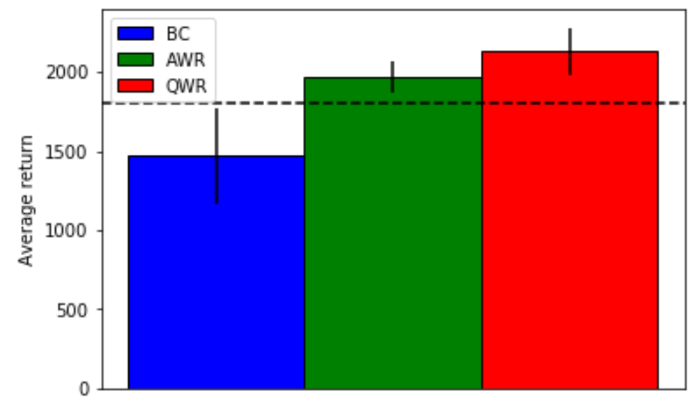
(a) HalfCheetah

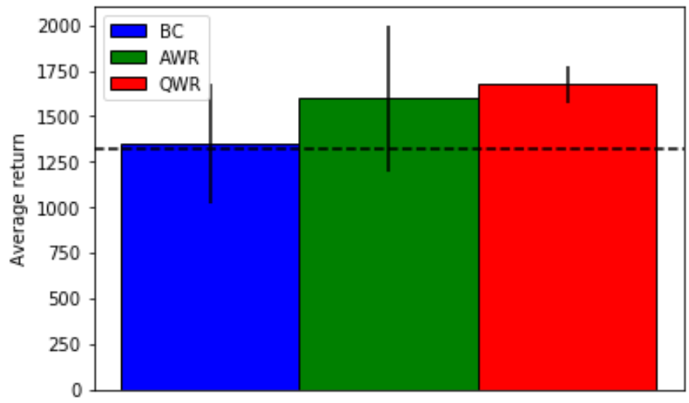
(b) Hopper

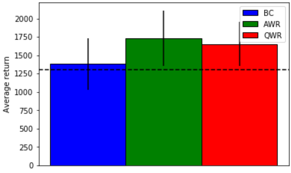
(c) Walker2d

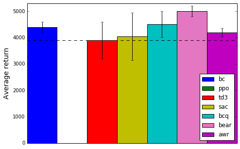
(d) HalfCheetah

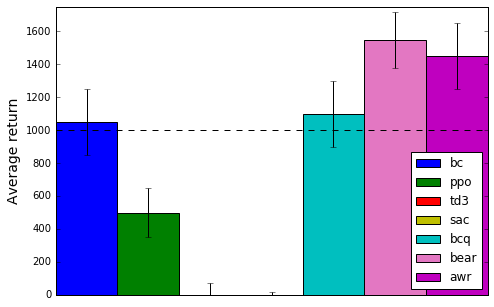
(e) Hopper

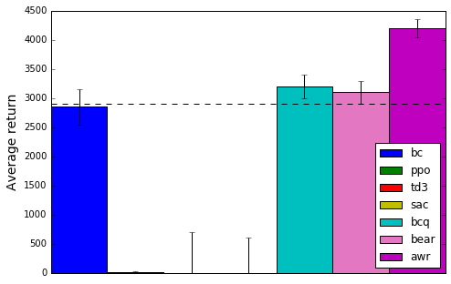
(f) Walker2d

Figure 3: Figures 3(a), 3(b) and 3(c) show offline trainings based on 50 trajectories of length 1000 collected by diverse policies. The horizontal lines mark the average return of a policy from the dataset. The bars denote median returns out of 4 runs, and the vertical lines denote the interquartile range. Data for figures 3(d), 3(e) and 3(f) is borrowed from Peng et al. (2019) to cover a broader family of algorithms and show that offline training fails for many RL algorithms.

For the offline RL experiments, we have trained each algorithm for 30 iterations, without additional data collection. The training trajectories contained only states, actions and rewards, without any algorithm-specific data. In QWR, we have set the per-step sampling policies $\mu$ to be Gaussians with mean at the performed action and standard deviation set to $0.4$, same as in Peng et al. (2019).

5 Discussion and Future Work

We present Q-value Weighted Regression (QWR), an off-policy actor-critic algorithm that extends Advantage Weighted Regression with action sampling and Q-learning. It is significantly more sample-efficient than AWR and works well with discrete actions and in visual domains, e.g., on Atari games. QWR consists of two interleaved steps of supervised training: the critic learning the Q function using a predefined backup operator, and the actor learning the policy with weighted regression based on multiple sampled actions. Thanks to this clear structure, QWR is simple to implement and debug. It is also stable in a wide range of hyperparameter choices and works well in the offline setting.

Importantly, we designed QWR thanks to a theoretical analysis that revealed why AWR may not work when there are limits on data collection in the environment. Our analysis for the limited data regime is based on the state-determines-action assumption that allows to fully solve AWR analytically while still being realistic and indicative of the performance of this algorithm with few samples. We believe that using the state-determines-action assumption can yield important insights into other RL algorithms as well.

QWR already achieves state-of-the-art results in settings with limited data and we believe that it can be further improved in the future. The critic training could benefit from the advances in Q-learning methods such as double Q-networks (van Hasselt et al., 2015) or Polyak averaging (Polyak, 1990), already used in SAC. Distributional Q-learning Bellemare et al. (2017) and the use of ensembles like REM Agarwal et al. (2020) could yield further improvements.

Notably, the QWR results at 100K that we present are achieved with the same set of hyperparameters (except for the network architecture) both for MuJoCo environments and for Atari games. This is rare among deep reinforcement learning algorithms, especially among ones that strive for sample-efficiency. Combined with its stability and good performance in offline settings, this makes QWR a compelling choice for reinforcement learning in domains with limited data.

6 Appendix

6.1 Experimental Details

We run experiments on 4 MuJoCo environments: Half-Cheetah, Walker, Hopper and Humanoid and on 6 Atari games: Boxing, Breakout, Freeway, Gopher, Pong and Seaquest. For the MuJoCo environments, we limit the episode length to $1000$. For the Atari environments, we apply the following preprocessing:

• Repeating each action for 4 consecutive steps, taking a maximum of 2 last frames as the observation.

• Stacking 4 last frames obtained from the previous step in one observation.

• Gray-scale observations, cropped and rescaled to size $84\times 84$.

• Maximum $10\mathrm{K}$ interactions per episode.

• Random number of no-op actions from range $[0..30]$ at the beginning of each episode.

• Rewards clipped to the $[-1,1]$ range during training.

Our code with the exact configurations we use to reproduce the experiments is available as open source. We use the same hyperparameters for the MuJoCo and Atari experiments, and almost the same hyperparameters for the 100K and 1M sample budgets. The hyperparameters and their tuning ranges are reported in Table 4.

Before calculating the actor loss, we normalize the advantages over the entire batch by subtracting their mean and dividing by their standard deviation, same as Peng et al. (2019). We perform a similar procedure for the log-sum-exp backup operator used in critic training. Before applying the backup, we divide the Q-values by a computed measure of their scale $s$. After applying the backup, we re-scale the target by $s$. There is no need to subtract the mean, as log-sum-exp is translation-invariant.

$$F(X)=\tau s(X)\log\left[\frac{1}{|X|}\sum_{x\in X}\exp\left(\frac{x}{\tau s(X)}\right)\right]$$ (6)

The parameters of this backup are the only ones different between the 100K and 1M experiments. For 100K, we use $\tau=0.3$ and mean absolute deviation as $s(X)$. For 1M, we use $\tau=1.0$ and standard deviation as $s(X)$.

Hyperparameter	Value	Considered range
$k$ - number of action samples	$4$	$\{2,4,8,32\}$
$T$ - multi-step target horizon (”margin”)	$3$	$\{1,3,7\}$
$\beta$ - actor loss temperature	$1$	$\{0.1,0.3,1,3,10\}$
$F$ - critic backup operator	log-sum-exp	mean, log-sum-exp, $\max$
$\gamma$ - discount factor for the returns	$0.99$	$\{0.99\}$
$\lambda$ - discount factor in TD($\lambda$)	$0.95$	$\{0.95\}$
$\alpha_{\pi}$ - actor learning rate	$1\text{\times}{10}^{-4}$	$\{$1\text{\times}{10}^{-4}$,$2\text{\times}{10}^{-4}$,$5\text{\times}{10}^{-4}$\}$
$\alpha_{V}$ - critic learning rate	$5\text{\times}{10}^{-4}$	$\{$2\text{\times}{10}^{-4}$,$5\text{\times}{10}^{-4}$,$1\text{\times}{10}^{-3}$\}$
batch size (actor and critic)	$256$	$\{128,256,512\}$
replay buffer size	$50\mathrm{K}$ interactions	$\{20\mathrm{K},50\mathrm{K},100\mathrm{K},200\mathrm{K}\}$
n_actor_steps	$1000$	$\{1000,2000,3000\}$
n_critic_steps	$1000$	$\{200,500,1000,2000\}$
update_frequency	$100$	$\{100,200,300\}$
n_iterations	Until we reach the desired number of interactions. In all experiments, we collect $1000$ interactions with the environment in each iteration of the algorithm.

Table 4: Hyperparameter values and considered ranges.

When training the networks, we use the Adam optimizer. We use the standard architectures for deep networks. In MuJoCo experiments we use a multi-layer perceptron with two layers 256 neurons each and ReLU activations. In Atari experiments we use the same convolutional architectures as Mnih et al. (2013a).

The 100K experiments took around 18 hours each, on a single TPU v2 chip. The 1M experiments took around 180 hours each, using the same hardware.

6.2 Formal Analysis of AWR with Limited Data

Since sample efficiency is one of the key challenges in deep reinforcement learning, it would be desirable to have better tools to understand why any RL algorithm – for instance AWR – is sample efficient or not. This is hard to achieve in the general setting, but we identify a key simplifying assumption that allows us to solve AWR analytically and identify the source of its problems.

The assumption we introduce, called state-determines-action, concerns the content of the replay buffer $\mathcal{D}$ of an off-policy RL algorithm. The replay buffer contains all state-action pairs that the algorithm has visited so far during its interactions with the environment. We say that a replay buffer $\mathcal{D}$ satisfies the state-determines-action assumption when for each state $s$ in the buffer, there is a unique action that was taken from it, formally:

$$\text{for all }(s,a),(s^{\prime},a^{\prime})\in\mathcal{D}:s=s^{\prime}\implies a=a^{\prime}.$$

A simplifying assumption like state-determines-action is useful only if it indeed simplifies the analysis of RL algorithms. We show that in case of AWR it does even more – it allows us to analytically calculate the final policy that the algorithm produces. In the case of AWR, it turns out that the resulting policy yields no improvement over the sampling policy.

While AWR achieves very good results after longer training, it is not very sample efficient, as noted in the future work section of (Peng et al., 2019). To address this problem, let us analyze a single loop of actor training in AWR:

$$\pi^{i+1}_{\mathcal{D}}\leftarrow\mathrm{argmax}_{\pi}\mathbb{E}_{\mathbf{s,a}\sim\mathcal{D}}\log\pi(\mathbf{a}|\mathbf{s})~{}\xi^{\mathbf{s,a}}_{\mathcal{D}},$$ (7)

$$\textrm{where}~{}\xi^{\mathbf{s,a}}_{\mathcal{D}}=\exp\left(\frac{1}{\beta}(\mathcal{R}_{\mathcal{D}}^{\mathbf{s,a}}-V^{i}_{\mathcal{D}}(\mathbf{s}))\right).$$ (8)

How does this update act on a replay buffer that satisfies the state-determines-action assumption? It turns out that we can answer this question analytically using the following theorem.

Theorem 1.

Let $\mathcal{A}$ be a discrete action space. Let a replay buffer $\mathcal{D}\subseteq\mathcal{S}\times\mathcal{A}$ satisfy the state-determines-action assumption. Let $\pi_{\mathcal{D}}$ be the probability function of a distribution that clones the behavior from $\mathcal{D}$, i.e., that assigns to each state $s$ from $\mathcal{D}$ the action $a$ such that $(s,a)\in\mathcal{D}$ with probability $1$. Then, under the AWR update, $\pi^{i+1}_{\mathcal{D}}\leftarrow\pi_{\mathcal{D}}$.

Proof.

By definition of the AWR update rule, $\pi^{i+1}_{\mathcal{D}}\leftarrow\mathrm{argmax}_{\pi}\mathbb{E}_{\mathbf{s,a}\sim\mathcal{D}}[\log\pi(\mathbf{a}|\mathbf{s})\xi^{\mathbf{s,a}}_{\mathcal{D}}]$. Recall that the number $\xi^{\mathbf{s,a}}_{\mathcal{D}}>0$ as an exponent of another number is always positive. Since $\mathcal{A}$ is a discrete action space, $\pi$ is a discrete policy and we have $\pi(\mathbf{a}|\mathbf{s})\leq 1$, so $\log\pi(\mathbf{a}|\mathbf{s})$ in the considered equation is at most 0 ($\log$ is a strictly increasing function and $\log(1)=0$). Thus the value $\log\pi(\mathbf{a}|\mathbf{s})~{}\xi^{\mathbf{s,a}}_{\mathcal{D}}$ can be at most $0$ and it reaches its maximum value for the policy that assigns probability $1$ to the action $a$ in state $s$ for each $(s,a)\in\mathcal{D}$. Therefore $\pi_{\mathcal{D}}$ attains the $\mathrm{argmax}_{\pi}$ as required. ∎

As we can see from the above theorem, the AWR update rule will insist on cloning the action taken in the replay buffer as long as it satisfies the state-determines-action assumption. In the extreme case of a deterministic environment, the new policy $\pi_{\mathcal{D}}$ will not add any new data to the buffer, only replay a trajectory already in it. So the whole AWR loop will end with the policy $\pi_{\mathcal{D}}$, which yields no improvement.

In the next section, we prove an analogous theorem for continuous action spaces.

6.2.1 Continuous action spaces

The statement of Theorem 1 must be adjusted for the case of continuous actions. First of all, let us clarify the notation of AWR update introduced in Equation 7:

$$\pi^{i+1}_{\mathcal{D}}\leftarrow\mathrm{argmax}_{\pi}\mathbb{E}_{\mathbf{s,a}\sim\mathcal{D}}\left[\log\pi(\mathbf{a}|\mathbf{s})~{}\xi^{\mathbf{s,a}}_{\mathcal{D}}\right]$$

For discrete actions, the symbol $\pi(\mathbf{a|s})$ denotes the probability function of a discrete distribution. In the continuous setting, we use it to denote probability density functions.

Now let us define the policy that ”clones the behavior from the replay buffer”. Intuitively that would be a distribution that concentrates most of its probability mass arbitrarily close to the action in the replay buffer.

Theorem 2.

Let $\mathcal{A}$ be a continuous action space. Let a replay buffer $\mathcal{D}\subseteq\mathcal{S}\times\mathcal{A}$ satisfy the state-determines-action assumption. For a given $\varepsilon>0$ let us consider the following family of parameterized Gaussian distributions

$$\pi_{\mu,\sigma}(\mathbf{a|s})=\frac{1}{\sigma(\mathbf{s})\sqrt{2\pi}}e^{-\frac{1}{2}(\frac{\mathbf{a}-\mu(\mathbf{s})}{\sigma(\mathbf{s})})^{2}},$$

where $\sigma(\mathbf{s})\geq\varepsilon$, and define $\pi_{\mathcal{D}}^{\epsilon}=\pi_{\mu,\sigma}$ such that $\sigma(\mathbf{s})=\varepsilon$ and $\mu(\mathbf{s})=\mathbf{a}~{}$ for $\mathbf{(s,a)}\in\mathcal{D}$. If we perform the optimization in the AWR update over such a family of distributions, we get $\pi^{i+1}_{\mathcal{D}}\leftarrow\pi_{\mathcal{D}}^{\epsilon}$.

Proof.

The reasoning is similar to the proof of Theorem 1 but we cannot rely on $\log\pi(\mathbf{a}|\mathbf{s})\leq 0$, as probability density functions can take arbitrarily large values. Let $s$ be any state that for some $a$ we have $(s,a)\in\mathcal{D}$. For the assumed family of distributions we have

$$\log\pi(a|s) =\log(\frac{1}{\sigma\sqrt{2\pi}})+\log(e^{-\frac{1}{2}(\frac{a-\mu}{\sigma})^{2}})=$$

$$=-\log(\sigma\sqrt{2\pi})-\frac{1}{2}(\frac{a-\mu}{\sigma})^{2}.$$

$\log\pi(a|s)$ is a quadratic function of $\mu$, so it attains the maximum value at $\mu=a$ for every $\sigma>0$. Now let’s look at

$$\frac{\partial}{\partial\sigma}\log(\frac{1}{\sigma\sqrt{2\pi}})=-\frac{1}{\sigma}<0.$$

The derivative is negative regardless of $\sigma$, so $\log\pi(\mathbf{a}|\mathbf{s})$ is maximized for the lowest allowed $\sigma(s)=\varepsilon$ and $\mu(s)=a$. This is true for arbitrary state-action pair such that $(s,a)\in\mathcal{D}$. So under the AWR update we get $\pi^{i+1}_{\mathcal{D}}\leftarrow\pi_{\mathcal{D}}^{\epsilon}$. ∎

This gives us intuition that the probability distributions $\pi(\mathbf{a|s})$ commonly used in RL (e.g. Gaussian) can be improved by increasing the density at $\mathbf{a}$ and decreasing it everywhere else. For those distributions, the maximum can come arbitrarily close to the Dirac delta, where $\pi(\mathbf{a}|\mathbf{s})=\infty$.

Given that AWR aims to copy the replay buffer, as demonstrated by Theorems 1 and 2, how come this algorithm works so well in practice, given enough interactions? First of all, note that for this effect to occur, the neural network used for AWR actor must be large enough and trained long enough to memorize the data from the replay buffer. Furthermore, the policy it learns must be allowed to express distributions that assign probability $1$ to a single action. This holds for environments with discrete actions, and for continuous actions with distributions with controlled scale, but it is not true e.g. when using Gaussian distributions with fixed variance. However, in the latter case, the proof of Theorem 2 shows that the AWR update will place the mean of the policy distribution at the performed action, regardless of the variance, which still leads to no improvement over the sampling policy.

In the next section, we show that using an algorithm, that corrects this cloning behavior, leads to improved sample efficiency.

6.3 Formal Analysis of QWR with Limited Data

To see how QWR performs under limited data, we are going to formulate a positive theorem showing that it achieves the policy improvement that AWR aims for even in a limited data setting. Note that this time we allow replay buffers that do not necessarily satisfy the state-determines-action assumption. But, for clarity, we make a simplifying assumption that the replay buffer has been sampled by a single policy $\mu$.

Recall the QWR update rule:

$$\begin{split}\pi^{i+1}_{\mathcal{D}}\leftarrow\mathrm{argmax}_{\pi}\mathbb{E}_{\mathbf{s}\sim\mathcal{D}}\mathbb{E}_{\mathbf{a}\sim\mu(\mathbf{\cdot|s})}\log\pi(\mathbf{a}|\mathbf{s})~{}\xi_{\mu}^{\mathbf{s,a}},\\ \begin{aligned} \textrm{where}~{}\xi_{\mu}^{\mathbf{s,a}}&=\exp\left(\frac{1}{\beta}(Q_{\mu}(\mathbf{s,a})-\hat{V}_{\mu}(\mathbf{s}))\right),\\ \hat{V}_{\mu}(\mathbf{s})~{}&=~{}\mathbb{E}_{a\sim\mu(\cdot|\mathbf{s})}Q_{\mu}(\mathbf{s,a}),\end{aligned}\end{split}$$ (9)

and $\mathcal{D}$ is the set of states in the replay buffer.

Let $\pi^{\star}_{\mu}(\mathbf{a|s})\propto\mu(\mathbf{a|s})\exp\left(\frac{1}{\beta}\left(\mathcal{R}_{\mathcal{\mu}}^{\mathbf{s,a}}-V_{\mu}(\mathbf{s})\right)\right)$, where $V_{\mu}$ is the state value function of $\mu$. This is the policy optimizing the expected improvement over the sampling policy $\mu$, subject to a KL constraint – the same as in Equation 36 in Peng et al. (2019).

Since $\pi_{\mu}^{\star}$ is the target policy resulting from the AWR derivation, we know from Peng et al. (2019) that AWR will update towards this policy in the limit, when the replay buffer is large enough. But from Theorem 1 we know that it will fail to perform this update when the state-determines-action assumption holds. Below we show that QWR will perform the same desirable update for any replay buffer, as long as we restrict the attention to states in the buffer.

Theorem 3.

Let $\mathcal{D}\subseteq\mathcal{S}$ be a finite sample from $d_{\mu}(\mathbf{s})$ - the undiscounted state distribution of a policy $\mu(\mathbf{a|s})$. Let $Q_{\mu}$ be the state-action value function for $\mu$, so $Q_{\mu}(\mathbf{s,a})=\mathcal{R}_{\mathcal{\mu}}^{\mathbf{s,a}}$ for any state and action. Then, under the QWR actor update, $\pi^{i+1}_{\mathcal{D}}\leftarrow\pi^{\star}_{\mu}|_{\mathcal{D}}$, where $\pi^{\star}_{\mu}|_{\mathcal{D}}$ is the policy $\pi^{\star}_{\mu}$. restricted to the set of states $\mathcal{D}$.

Proof.

Let $s$ be an arbitrary state in $\mathcal{D}$. From the definition of $\hat{V}_{\mu}(\mathbf{s})$ we have

$$\hat{V}_{\mu}(\mathbf{s})~{}=~{}\mathbb{E}_{a\sim\mu(\cdot|\mathbf{s})}Q_{\mu}(\mathbf{s,a})=V_{\mu}(\mathbf{s}).$$

Since $Q_{\mu}(\mathbf{s,a})=\mathcal{R}_{\mathcal{\mu}}^{\mathbf{s,a}}$,

$$\begin{split}\pi^{i+1}_{\mathcal{D}}\leftarrow~{}&\mathrm{argmax}_{\pi}\mathbb{E}_{\mathbf{s}\sim\mathcal{D}}\mathbb{E}_{\mathbf{a}\sim\mu(\mathbf{\cdot|s})}\log\pi(\mathbf{a}|\mathbf{s})~{}\xi_{\mu}^{\mathbf{s,a}}\\ \textrm{where}~{}\xi_{\mu}^{\mathbf{s,a}}&=\exp\left(\frac{1}{\beta}(\mathcal{R}_{\mathcal{\mu}}^{\mathbf{s,a}}-V_{\mu}(\mathbf{s}))\right).\end{split}$$ (10)

We can now change the measure using the definition of $\pi^{\star}$:

$$\pi^{i+1}_{\mathcal{D}}\leftarrow\mathrm{argmax}_{\pi}\mathbb{E}_{\mathbf{s}\sim\mathcal{D}}\mathbb{E}_{\mathbf{a}\sim\pi^{\star}(\mathbf{\cdot|s})}\log\pi(\mathbf{a}|\mathbf{s})\mathrm{.}$$ (11)

The inner expectation, up to a normalizing constant, is the negative cross-entropy between $\pi^{\star}$ and $\pi$. Since cross-entropy between two distributions is minimized when the distributions are equal, the optimum is reached at $\pi=\pi^{\star}_{\mu}|_{\mathcal{D}}$ for all $s\in\mathcal{D}$. ∎

As we can see, the QWR update rule reaches the desired target policy even under limited data. This stands in contrast to AWR, which requires repeating states in the replay buffer, as shown in Theorems 1 and 2.

6.4 Multi-step targets

To make the training of the Q-value network more efficient, we implement an approach inspired by widely-used multi-step Q-learning (Mnih et al., 2016). We consider targets for the Q-value network computed over multiple different time horizons:

$$\begin{split}Q^{\star}_{\mu,t}(\mathbf{s}_{i},\mathbf{a}_{i})=&\left(\sum_{j=i}^{i+t-1}\gamma^{j}\mathbf{r}_{j}\right)+\gamma^{i+t}\mathbb{E}_{\mathbf{a}^{\prime}_{1},...,\mathbf{a}^{\prime}_{n}\sim\mu(\cdot|\mathbf{s}_{i+t})}\\ &F(\{Q_{\mu}(\mathbf{s}_{t+1},\mathbf{a}^{\prime}_{1}),...,Q_{\mu}(\mathbf{s}_{t+1},\mathbf{a}^{\prime}_{n})\})\end{split}$$ (12)

where $\mathbf{s}_{i}$, $\mathbf{a}_{i}$, $\mathbf{r}_{i}$ are the states, actions and rewards in a collected trajectory, respectively. We aggregate those multi-step targets using a truncated TD($\lambda$) estimator (Sutton & Barto, 2018, p. 236):

$$Q^{\star}_{\mu}(\mathbf{s,a})=(1-\lambda)\sum_{t=1}^{T}\lambda^{t-1}Q^{\star}_{\mu,t}(\mathbf{s,a})$$ (13)

References

- Abdolmaleki et al. (2018) Abdolmaleki, A., Springenberg, J. T., Tassa, Y., Munos, R., Heess, N., and Riedmiller, M. A. Maximum a posteriori policy optimisation. CoRR, abs/1806.06920, 2018. URL http://arxiv.org/abs/1806.06920.
- Agarwal et al. (2019) Agarwal, R., Schuurmans, D., and Norouzi, M. Striving for simplicity in off-policy deep reinforcement learning. CoRR, abs/1907.04543, 2019. URL http://arxiv.org/abs/1907.04543.
- Agarwal et al. (2020) Agarwal, R., Schuurmans, D., and Norouzi, M. An optimistic perspective on offline reinforcement learning, 2020.
- Bartlett et al. (2017) Bartlett, P. L., Foster, D. J., and Telgarsky, M. J. Spectrally-normalized margin bounds for neural networks. In Guyon, I., Luxburg, U. V., Bengio, S., Wallach, H., Fergus, R., Vishwanathan, S., and Garnett, R. (eds.), Advances in Neural Information Processing Systems, volume 30, pp. 6240–6249. Curran Associates, Inc., 2017. URL https://proceedings.neurips.cc/paper/2017/file/b22b257ad0519d4500539da3c8bcf4dd-Paper.pdf.
- Bellemare et al. (2017) Bellemare, M. G., Dabney, W., and Munos, R. A distributional perspective on reinforcement learning, 2017.
- Fujimoto et al. (2018) Fujimoto, S., Meger, D., and Precup, D. Off-policy deep reinforcement learning without exploration. CoRR, abs/1812.02900, 2018. URL http://arxiv.org/abs/1812.02900.
- Ghasemipour et al. (2020) Ghasemipour, S. K. S., Schuurmans, D., and Gu, S. S. Emaq: Expected-max q-learning operator for simple yet effective offline and online rl, 2020.
- Haarnoja et al. (2018) Haarnoja, T., Zhou, A., Abbeel, P., and Levine, S. Soft actor-critic: Off-policy maximum entropy deep reinforcement learning with a stochastic actor, 2018.
- Hessel et al. (2017) Hessel, M., Modayil, J., van Hasselt, H., Schaul, T., Ostrovski, G., Dabney, W., Horgan, D., Piot, B., Azar, M. G., and Silver, D. Rainbow: Combining improvements in deep reinforcement learning. CoRR, abs/1710.02298, 2017. URL http://arxiv.org/abs/1710.02298.
- Kaiser et al. (2019) Kaiser, L., Babaeizadeh, M., Milos, P., Osinski, B., Campbell, R. H., Czechowski, K., Erhan, D., Finn, C., Kozakowski, P., Levine, S., Sepassi, R., Tucker, G., and Michalewski, H. Model-based reinforcement learning for atari. CoRR, abs/1903.00374, 2019. URL http://arxiv.org/abs/1903.00374.
- Kumar et al. (2020) Kumar, A., Zhou, A., Tucker, G., and Levine, S. Conservative q-learning for offline reinforcement learning, 2020.
- Levine (2018) Levine, S. Reinforcement learning and control as probabilistic inference: Tutorial and review, 2018.
- Levine et al. (2020) Levine, S., Kumar, A., Tucker, G., and Fu, J. Offline reinforcement learning: Tutorial, review, and perspectives on open problems, 2020.
- Lillicrap et al. (2015) Lillicrap, T. P., Hunt, J. J., Pritzel, A., Heess, N., Erez, T., Tassa, Y., Silver, D., and Wierstra, D. Continuous control with deep reinforcement learning, 2015.
- Mnih et al. (2013a) Mnih, V., Kavukcuoglu, K., Silver, D., Graves, A., Antonoglou, I., Wierstra, D., and Riedmiller, M. Playing atari with deep reinforcement learning, 2013a.
- Mnih et al. (2013b) Mnih, V., Kavukcuoglu, K., Silver, D., Graves, A., Antonoglou, I., Wierstra, D., and Riedmiller, M. Playing atari with deep reinforcement learning, 2013b.
- Mnih et al. (2016) Mnih, V., Badia, A. P., Mirza, M., Graves, A., Lillicrap, T. P., Harley, T., Silver, D., and Kavukcuoglu, K. Asynchronous methods for deep reinforcement learning, 2016.
- Munos et al. (2016) Munos, R., Stepleton, T., Harutyunyan, A., and Bellemare, M. G. Safe and efficient off-policy reinforcement learning. CoRR, abs/1606.02647, 2016. URL http://arxiv.org/abs/1606.02647.
- Nair et al. (2020) Nair, A., Dalal, M., Gupta, A., and Levine, S. Accelerating online reinforcement learning with offline datasets, 2020.
- Neumann & Peters (2009) Neumann, G. and Peters, J. R. Fitted q-iteration by advantage weighted regression. In Koller, D., Schuurmans, D., Bengio, Y., and Bottou, L. (eds.), Advances in Neural Information Processing Systems 21, pp. 1177–1184. Curran Associates, Inc., 2009. URL http://papers.nips.cc/paper/3501-fitted-q-iteration-by-advantage-weighted-regression.pdf.
- OpenAI (2018) OpenAI. Openai five. https://blog.openai.com/openai-five/, 2018.
- OpenAI et al. (2018) OpenAI, Andrychowicz, M., Baker, B., Chociej, M., Józefowicz, R., McGrew, B., Pachocki, J. W., Pachocki, J., Petron, A., Plappert, M., Powell, G., Ray, A., Schneider, J., Sidor, S., Tobin, J., Welinder, P., Weng, L., and Zaremba, W. Learning dexterous in-hand manipulation. CoRR, abs/1808.00177, 2018. URL http://arxiv.org/abs/1808.00177.
- Peng et al. (2019) Peng, X. B., Kumar, A., Zhang, G., and Levine, S. Advantage-weighted regression: Simple and scalable off-policy reinforcement learning, 2019.
- Peters & Schaal (2007) Peters, J. and Schaal, S. Reinforcement learning by reward-weighted regression for operational space control. In Proceedings of the 24th International Conference on Machine Learning, ICML ’07, pp. 745–750, New York, NY, USA, 2007. Association for Computing Machinery. ISBN 9781595937933. doi: 10.1145/1273496.1273590. URL https://doi.org/10.1145/1273496.1273590.
- Polyak (1990) Polyak, B. New method of stochastic approximation type. Automation and Remote Control, 1990, 01 1990.
- Rusu et al. (2016) Rusu, A. A., Vecerík, M., Rothörl, T., Heess, N., Pascanu, R., and Hadsell, R. Sim-to-real robot learning from pixels with progressive nets. CoRR, abs/1610.04286, 2016. URL http://arxiv.org/abs/1610.04286.
- Sadeghi & Levine (2016) Sadeghi, F. and Levine, S. (cad)$^2$rl: Real single-image flight without a single real image. CoRR, abs/1611.04201, 2016. URL http://arxiv.org/abs/1611.04201.
- Schulman et al. (2017) Schulman, J., Wolski, F., Dhariwal, P., Radford, A., and Klimov, O. Proximal policy optimization algorithms, 2017.
- Schwarzer et al. (2020) Schwarzer, M., Anand, A., Goel, R., Hjelm, R. D., Courville, A., and Bachman, P. Data-efficient reinforcement learning with momentum predictive representations, 2020.
- Siegel et al. (2020) Siegel, N. Y., Springenberg, J. T., Berkenkamp, F., Abdolmaleki, A., Neunert, M., Lampe, T., Hafner, R., Heess, N., and Riedmiller, M. Keep doing what worked: Behavioral modelling priors for offline reinforcement learning, 2020.
- Silver et al. (2017) Silver, D., Hubert, T., Schrittwieser, J., Antonoglou, I., Lai, M., Guez, A., Lanctot, M., Sifre, L., Kumaran, D., Graepel, T., Lillicrap, T. P., Simonyan, K., and Hassabis, D. Mastering chess and shogi by self-play with a general reinforcement learning algorithm. CoRR, abs/1712.01815, 2017. URL http://arxiv.org/abs/1712.01815.
- Sutton & Barto (2018) Sutton, R. S. and Barto, A. G. Reinforcement Learning: An Introduction. A Bradford Book, Cambridge, MA, USA, 2018. ISBN 0262039249.
- Sutton et al. (1999) Sutton, R. S., McAllester, D., Singh, S., and Mansour, Y. Policy gradient methods for reinforcement learning with function approximation. In Proceedings of the 12th International Conference on Neural Information Processing Systems, NIPS’99, pp. 1057–1063, Cambridge, MA, USA, 1999. MIT Press.
- Sutton et al. (2000) Sutton, R. S., McAllester, D. A., Singh, S. P., and Mansour, Y. Policy gradient methods for reinforcement learning with function approximation. In Solla, S. A., Leen, T. K., and Müller, K. (eds.), Advances in Neural Information Processing Systems 12, pp. 1057–1063. MIT Press, 2000.
- Szegedy et al. (2014) Szegedy, C., Zaremba, W., Sutskever, I., Bruna, J., Erhan, D., Goodfellow, I., and Fergus, R. Intriguing properties of neural networks. In International Conference on Learning Representations, 2014. URL http://arxiv.org/abs/1312.6199.
- van Hasselt et al. (2015) van Hasselt, H., Guez, A., and Silver, D. Deep reinforcement learning with double q-learning, 2015.
- van Hasselt et al. (2019) van Hasselt, H., Hessel, M., and Aslanides, J. When to use parametric models in reinforcement learning? CoRR, abs/1906.05243, 2019. URL http://arxiv.org/abs/1906.05243.
- Vinyals et al. (2017) Vinyals, O., Ewalds, T., Bartunov, S., Georgiev, P., Vezhnevets, A. S., Yeo, M., Makhzani, A., Küttler, H., Agapiou, J., Schrittwieser, J., Quan, J., Gaffney, S., Petersen, S., Simonyan, K., Schaul, T., van Hasselt, H., Silver, D., Lillicrap, T. P., Calderone, K., Keet, P., Brunasso, A., Lawrence, D., Ekermo, A., Repp, J., and Tsing, R. Starcraft II: A new challenge for reinforcement learning. CoRR, abs/1708.04782, 2017. URL http://arxiv.org/abs/1708.04782.
- Wang et al. (2018) Wang, Q., Xiong, J., Han, L., sun, p., Liu, H., and Zhang, T. Exponentially weighted imitation learning for batched historical data. In Bengio, S., Wallach, H., Larochelle, H., Grauman, K., Cesa-Bianchi, N., and Garnett, R. (eds.), Advances in Neural Information Processing Systems 31, pp. 6288–6297. Curran Associates, Inc., 2018.
- Wang et al. (2020) Wang, Z., Novikov, A., Zolna, K., Springenberg, J. T., Reed, S., Shahriari, B., Siegel, N., Merel, J., Gulcehre, C., Heess, N., and de Freitas, N. Critic regularized regression, 2020.
- Williams (1992) Williams, R. J. Simple statistical gradient-following algorithms for connectionist reinforcement learning. Mach. Learn., 8(3–4):229–256, May 1992. ISSN 0885-6125. doi: 10.1007/BF00992696. URL https://doi.org/10.1007/BF00992696.
- Wirth et al. (2016) Wirth, C., Fürnkranz, J., and Neumann, G. Model-free preference-based reinforcement learning. In Schuurmans, D. and Wellman, M. P. (eds.), Proceedings of the Thirtieth AAAI Conference on Artificial Intelligence, February 12-17, 2016, Phoenix, Arizona, USA, pp. 2222–2228. AAAI Press, 2016. URL http://www.aaai.org/ocs/index.php/AAAI/AAAI16/paper/view/12247.
- Zhang et al. (2016) Zhang, C., Bengio, S., Hardt, M., Recht, B., and Vinyals, O. Understanding deep learning requires rethinking generalization. 2016. URL http://arxiv.org/abs/1611.03530. cite arxiv:1611.03530Comment: Published in ICLR 2017.