Newton Method over Networks is Fast up to the Statistical Precision

Abstract

We propose a distributed cubic regularization of the Newton method for solving (constrained) empirical risk minimization problems over a network of agents, modeled as undirected graph. The algorithm employs an inexact, preconditioned Newton step at each agent’s side: the gradient of the centralized loss is iteratively estimated via a gradient-tracking consensus mechanism and the Hessian is subsampled over the local data sets. No Hessian matrices are thus exchanged over the network. We derive global complexity bounds for convex and strongly convex losses. Our analysis reveals an interesting interplay between sample and iteration/communication complexity: statistically accurate solutions are achievable roughly in the same number of iterations of the centralized cubic Newton, with a communication cost per iteration of the order of $\widetilde{\mathcal{O}}\big{(}1/\sqrt{1-\rho}\big{)}$, where $\rho$ characterizes the connectivity of the network. This represents a significant communication saving with respect to that of existing, statistically oblivious, distributed Newton-based methods over networks.

1 Introduction

We study Empirical Risk Minimization (ERM) problems over a network of $m$ agents, modeled as undirected graph. Differently from master/slave systems, no centralized node is assumed in the network (which will be referred to as meshed network). Each agent $i$ has access to $n$ i.i.d. samples $z_{i}^{(1)},\ldots,z_{i}^{(n)}$ drawn from an unknown, common distribution on $\mathcal{Z}\subseteq\mathbb{R}^{p}$; the associated empirical risk reads

$$f_{i}(x)\triangleq\frac{1}{n}\sum_{j=1}^{n}\ell\big{(}x;z_{i}^{(j)}\big{)},\vspace{-0.1cm}\vspace{-0.1cm}$$ (1)

where $\ell:\mathbb{R}^{d}\times\mathcal{Z}\to\mathbb{R}$ is the loss function, assumed to be (strongly) convex in $x$, for any given $z\in\mathcal{Z}$. Agents aim to minimize the total empirical risk over the $N\!=mn$ samples, resulting in the following ERM over networks:

$$\widehat{x}\in\underset{x\in\mathcal{K}}{\text{argmin}}\,F\left(x\right)\triangleq\frac{1}{m}\sum_{i=1}^{m}f_{i}\left(x\right),\vspace{-0.2cm}$$ (P)

where $\mathcal{K}\!\subseteq\mathbb{R}^{d}$ is convex and known to the agents.

Since the functions $f_{i}$ can be accessed only locally and routing local data to other agents is infeasible or highly inefficient, solving (P) calls for the design of distributed algorithms that alternate between a local computation procedure at each agent’s side, and a round of communication among neighboring nodes. The cost of communications is often considered the bottleneck for distributed computing, if compared with local (possibly parallel) computations (e.g., (Bekkerman et al., 2011; Lian et al., 2017)). Therefore, our goal is developing communication-efficient distributed algorithms that solve (P) within the statistical precision.

The provably faster convergence rates of second order methods over gradient-based algorithms make them potential candidates for communication saving (at the cost of more computations). Despite the success of Newton-like methods to solve ERM in a centralized setting (e.g., (Mokhtari et al., 2016a; Bottou et al., 2018)), including master/slave architectures (Zhang & Xiao, 2015; Shamir et al., 2014; Ma & Takac, 2017; Jahani et al., 2020; Soori et al., 2020), their distributed counterparts on meshed networks are not on par: convergence rates provably faster than those of first order methods are achieved at high communication costs (Uribe & Jadbabaie, 2020a; Zhang et al., 2020), cf. Sec. 1.2.

We claim that stronger guarantees of second order methods over meshed networks can be certified if a statistically-informed design/analysis is put forth, in contrast with statistically agnostic approaches that look at (P) as deterministic optimization and target any arbitrarily small suboptimality. To do so, we build on the following two key insights.

$\bullet$ Fact 1 (statistical accuracy): When it comes to learning problems, the ERM (P) is a surrogate of the population minimization

$$x^{\star}\in\underset{x\in\mathcal{K}}{\text{argmin}}\,F_{P}\left(x\right)\triangleq\mathbb{E}_{Z\sim\mathbb{P}}\,\ell\left(x;Z\right).\vspace{-0.1cm}$$ (2)

The ultimate goal is to estimate ${x}^{\star}$ via the ERM (P). Denoting by $x_{\varepsilon}\in\mathcal{K}$ the estimate returned by the algorithm, we have the risk decomposition (neglecting the approximation error due to the use of a specific set of models $x\in\mathcal{K}$):

$$\begin{array}[]{lll}&F_{P}(x_{\varepsilon})-F_{P}(x^{\star})\vskip 6.0pt plus 2.0pt minus 2.0pt\\ &=\underset{\leq\text{statistical error}}{\big{\{}F_{P}(x_{\varepsilon})-F(x_{\varepsilon})\big{\}}}\vskip 6.0pt plus 2.0pt minus 2.0pt+{\big{\{}F(x_{\varepsilon})-F(x^{\star})\big{\}}}\\ &\quad+\underset{\leq\text{statistical error}}{\big{\{}F(x^{\star})-F_{P}(x^{\star})\big{\}}}\vskip 6.0pt plus 2.0pt minus 2.0pt\\ &\leq\mathcal{O}(\text{statistical error})+\underset{=\text{optimization error}}{\big{\{}F(x_{\varepsilon})-F(\widehat{x})\big{\}}}\vspace{-.2cm}\end{array}$$ (3)

where the statistical error is usually of the order $\mathcal{O}(1/\!\sqrt{N})$ or $\mathcal{O}(1/N)$ (cf. Sec. 2). It is thus sufficient to reach an optimization accuracy $F(x_{\varepsilon})-F(\widehat{x})=\mathcal{O}(\text{statistical error})$. This can potentially save communications.

$\bullet$ Fact 2 (statistical similarity): Under mild assumptions on the loss functions and i.i.d samples across the agents (e.g., (Zhang & Xiao, 2015; Hendrikx et al., 2020b)), it holds with high probability (and uniformly on $\mathcal{Z}$)

$$\left\|\nabla^{2}f_{i}(x)-\nabla^{2}F(x)\right\|\leq{\beta}=\widetilde{\mathcal{O}}(1/\sqrt{n}),\;\;\forall x\in\mathcal{K},\vspace{-0.1cm}$$ (4)

with $\widetilde{\mathcal{O}}$ hiding log-factors and the dependence on $d$. In words, the local empirical losses $f_{i}$ are statistically similar to each other and the average $F$, especially for large $n$.

The key insight of Fact 1 is that one can target suboptimal solutions of (P) within the statistical error. This is different from seeking a distributed optimization method that achieves any arbitrarily small empirical suboptimality. Fact 2 suggests a further reduction in the communication complexity via statistical preconditioning, that is, subsampling the Hessian of $F$ over the local data sets, so that no Hessian matrix has to be transmitted over the network. This paper shows that, if synergically combined, these two facts can improve the communication complexity of distributed second order methods over meshed networks.

1.1 Major contributions

We propose and analyze a decentralization of the cubic regularization of the Newton method (Nesterov & Polyak, 2006) over meshed networks. The algorithm employs a local computation procedure performed in parallel by the agents coupled with a round of (perturbed) consensus mechanisms that aim to track locally the gradient of $F$ (a.k.a. gradient-tracking) as well as enforce an agreement on the local optimization directions. The optimization procedure is an inexact, preconditioned (cubic regularized) Newton step whereby the gradient of $F$ is estimated by gradient tracking while the Hessian of $F$ is subsampled over the local data sets. Neither a line-search nor communication of Hessian matrices over the network are performed.

We established for the first time global convergence for different classes of ERM problems, as summarized in Table 1.1. Our results are of two types: i) classical complexity analysis (number of communication rounds) for arbitrary solution accuracy (right panel); ii) and complexity bounds for statistically optimal solutions (left panel, $V_{N}$ is the statistical error). Postponing to Sec 4 a detailed discussion of these results, here we highlight some key novelties of our findings. Convex ERM: For convex $F$, if arbitrary $\varepsilon$-solutions are targeted, the algorithm exhibits a two-speed behavior: 1) a first rate of the order of $\mathcal{O}((1/\sqrt{1-\rho})\cdot\sqrt{LD^{3}/\varepsilon^{1+\alpha}})$, as long as $\varepsilon=\Omega(LD^{3}\beta^{2})$; up to the network dependent factor $1/\sqrt{1-\rho}$, this (almost) matches the rate of the centralized Newton method (Nesterov & Polyak, 2006); and 2) the slower rate $\mathcal{O}(({1}/{\sqrt{1-\rho}})\cdot(LD^{3}\beta^{2})/\varepsilon)$, which is due to the local subsampling of the global Hessian $\nabla^{2}F$; this term is dominant for smaller values of $\varepsilon$. The interesting fact is that $\varepsilon=\Omega(LD^{3}\beta^{2})$ is of the order of the statistical error $V_{N}$. Therefore, rates of the order of centralized ones are provably achieved up to statistical precision (left panel). Strongly Convex ERM ($\beta<\mu$): The communication complexity shows a three-phase rate behaviour (right panel); for arbitrarily small $\varepsilon>0$, the worst-case communication complexity is linear, of the order of $\widetilde{\mathcal{O}}\big{(}({1}/{\sqrt{1-\rho}})\cdot(\beta/\mu)\cdot\log(1/\varepsilon)\big{)}$. Faster rates are certified when $\varepsilon=\mathcal{O}(V_{N})$ (left panel). Note that the region of superlinear convergence is a false improvement when the first term $m^{1/4}\sqrt{LD/\mu}$ is dominant, e.g., $F$ is ill-conditioned and $n$ is not large. This term is unavoidable (Nesterov & Polyak, 2006)–unless more refined function classes are considered, such as self-concordant or quadratic ($L=0$). The left panel shows improved rates in the latter case or under an initialization within a $\mathcal{O}(1/\sqrt{n})$-neighborhood of the solution. Strongly Convex ERM ($\beta\geq\mu$): This is a common setting when $F_{P}$ is convex and a regularizer is used in the ERM (P) for learnability/stability purposes; typically, $\mu=\mathcal{O}(1/\sqrt{N})$, $\beta=\mathcal{O}(1/\sqrt{n})$. We proved linear rate for arbitrary $\varepsilon$-values. Differently from the majority of first-order methods over meshed networks (cf. Sec. 1.2), this rate does not depend on the condition number of $F$ but on the generally more favorable ratio $\beta/\mu$. Furthermore, when $\varepsilon=\mathcal{O}(V_{N})$, the rate does not improve over the convex case.
In summary, we propose a second-order method solving convex and strongly convex problems over meshed networks that, for the first time, enjoys global complexity bounds and communication complexity close to oracle complexity of centralized methods up to the statistical precision.

Table 1: Communication complexity of DiRegINA to $\varepsilon>0$ suboptimality for (strongly) convex ERM. Right column: arbitrary $\varepsilon$ values. Left column: $\varepsilon=\Omega(V_{N})$, $V_{N}$ is the statistical error [cf. (3)]. The other parameters are: $\mu$ and $L$ are the strong convexity constant of $F$ and Lipschitz constant of $\nabla^{2}F$, respectively; $D$ and $D_{p}$ are estimates of the optimality gap at the initial point; $\beta$ measures the similarity of $\nabla^{2}f_{i}$ [cf. (4)]; $\rho$ characterizes the connectivity of the network; and $\alpha>0$ is an arbitrarily small constant.

Problem		$\varepsilon=\Omega(V_{N})$ (statistical error)	$\varepsilon>0$ (arbitrary)
Convex  $\mu=0$ $V_{N}={\mathcal{O}}(1/{\sqrt{N}})$	Thm. 7 Cor. 8	$\widetilde{\mathcal{O}}\left({\frac{1}{\sqrt{1-\rho}}\cdot\sqrt{\frac{LD^{3}}{V_{N}^{1+\alpha}}}}\right)$	$\widetilde{\mathcal{O}}\bigg{(}\frac{1}{\sqrt{1-\rho}}\cdot\left\{\sqrt{\frac{LD^{3}}{\varepsilon^{1+\alpha}}}+\frac{LD^{3}\beta}{\varepsilon^{1+\alpha/2}}\right\}\bigg{)}$
	$L>0$ Thm. 9 Cor.10	$\widetilde{\mathcal{O}}\bigg{(}\frac{1}{\sqrt{1-\rho}}\Big{\{}m^{1/4}\sqrt{\frac{LD}{\mu}}+\log\log\left(\frac{\mu^{3}}{mL^{2}V_{N}}\right)\Big{\}}\bigg{)}$	$\widetilde{\mathcal{O}}\bigg{(}\frac{1}{\sqrt{1-\rho}}\Big{\{}m^{1/4}\cdot\sqrt{\frac{LD}{\mu}}+\log\log\left(\frac{\mu^{2}}{\beta^{2}}\min\left\{1,\frac{\beta^{2}\mu}{mL^{2}}\cdot\frac{1}{\varepsilon}\right\}\right)$
Strongly-convex $0<\beta<\mu$ $V_{N}={\mathcal{O}}({1}/{N})$ $\mu=\mathcal{O}(1)$			$+\frac{\beta}{\mu}\log\left(\frac{\beta^{2}\mu}{mL^{2}\varepsilon}\right)\Big{\}}\bigg{)}$
	$L>0$ +initialization (Cor. 11)	$\widetilde{\mathcal{O}}\left({\frac{1}{\sqrt{1-\rho}}\cdot\left\{\log\log\left(\frac{\mu^{3}}{mL^{2}}\cdot\frac{1}{V_{N}}\right)\right\}}\right),\quad\beta=\mathcal{O}\left(\frac{1}{\sqrt{n}}\right)$	$\widetilde{\mathcal{O}}\left({\frac{1}{\sqrt{1-\rho}}\left\{\log\log\left(\frac{\mu^{2}}{\beta^{2}}\cdot\min\left(1,\frac{\beta^{2}\mu}{mL^{2}\varepsilon}\right)\right)+\frac{\beta}{\mu}\log\left(\frac{\beta^{2}\mu}{mL^{2}\varepsilon}\right)\right\}}\right)$
	$L=0$ (Thm. 18, appendix E.4)	$\widetilde{\mathcal{O}}\left(\frac{1}{\sqrt{1-\rho}}\cdot\log\log\left(\frac{D_{p}}{V_{N}}\right)\right),\quad\beta=\mathcal{O}\left(\frac{1}{\sqrt{n}}\right)$	$\widetilde{\mathcal{O}}\left({\frac{1}{\sqrt{1-\rho}}\cdot\left\{\log\log\left(\frac{D_{p}}{\varepsilon}\right)+\frac{\beta}{\mu}\log\left(\frac{D_{p}\beta^{2}}{\mu^{2}\varepsilon}\right)\right\}}\right)$
Strongly-convex (regularized) $0<\mu\leq\beta$ $V_{N}={\mathcal{O}}({1}/\sqrt{N})$	$L>0$ (Thm. 12)	$\widetilde{\mathcal{O}}\bigg{(}\frac{1}{\sqrt{1-\rho}}m^{1/2}\sqrt{\frac{LD}{V_{N}}}\bigg{)},\quad\left\{\begin{array}[]{cc}&\mu=\mathcal{O}(V_{N})\\ &\beta=\mathcal{O}(\frac{1}{\sqrt{n}})\end{array}\right.$	$\widetilde{\mathcal{O}}\bigg{(}\frac{1}{\sqrt{1-\rho}}\left\{\sqrt{\frac{LD}{\mu}}\left(1+m^{1/4}\sqrt{\frac{\beta}{\mu}}\right)+\frac{\beta}{\mu}\log\Big{(}\frac{\beta^{2}\mu}{mL^{2}\varepsilon}\Big{)}\right\}\bigg{)}$
	$L=0$ (Thm. 19, appendix G)	$\widetilde{\mathcal{O}}\left(\frac{1}{\sqrt{1-\rho}}\cdot m^{1/2}\cdot\log\left(\frac{1}{V_{N}}\right)\right),\quad\left\{\begin{array}[]{cc}&\mu=\mathcal{O}(V_{N})\\ &\beta=\mathcal{O}(\frac{1}{\sqrt{n}})\end{array}\right.$	$\widetilde{\mathcal{O}}\left(\frac{1}{\sqrt{1-\rho}}\cdot\frac{\beta}{\mu}\cdot\log\left(\frac{1}{\varepsilon}\right)\right)$

1.2 Related Works

The literature of distributed optimization is vast; here we review relevant methods applicable to meshed networks, omitting the less relevant work considering only master-slave systems (a.k.a star networks). $\bullet$ Statistically oblivious methods: Despite being vast and providing different communication and oracle complexity bounds, the literature (e.g., (Jakovetić et al., 2014; Shi et al., 2015; Arjevani & Shamir, 2015; Nedic et al., 2017; Scaman et al., 2017; Lan et al., 2017; Uribe et al., 2020; Rogozin et al., 2020)) on decentralized first-order methods for minimizing $Q$-Lipschitz-smooth and $\mu$-strongly convex global objective $F$ mostly focuses on the particular case where $n=1$ in (1) and $\mathcal{K}=\mathbb{R}^{d}$, and does not take into account statistical similarity of the risks. The best convergence results for nonaccelerated first-order methods certify linear rate, scaling with the condition number $\kappa=Q/\mu$ ($Q$ is the Lipschitz constant of $\nabla F$); Nesterov-based acceleration improves the dependence to $\sqrt{\kappa}$ (Gorbunov et al., 2020). This performance can still be unsatisfactory when $1+\beta/\mu<\kappa$ (resp. $1+\beta/\mu<\sqrt{\kappa}$). This is the typical situation of ill-conditioned problems, such as many learning problems where the regularization parameter that is optimal for test predictive performance is very small (Hendrikx et al., 2020b). For instance, consider the ridge-regression problem with optimal regularization parameter $\mu=1/\sqrt{mn}$ (Table 1 in (Zhang & Xiao, 2015)), we have: $\kappa=\mathcal{O}(\sqrt{m\cdot n})$ while $\beta/\mu=\mathcal{O}(\sqrt{m})$. Notice that the former grows with the local sample size $n$, while the latter is independent.

A number of second-order methods were proposed for distributed optimization over meshed networks, with typical results being local superlinear convergence (Jadbabaie et al., 2009; Wei et al., 2013; Tutunov et al., 2019) or global linear convergence no better than that of first-order methods (Mokhtari et al., 2016d, 2017, c; Eisen et al., 2019; Jiaojiao et al., 2020). Improved upon first-order methods global bounds are achieved by exploiting expensive sending local Hessians over the network–such as (Zhang et al., 2020), obtaining communication complexity bound ${\mathcal{O}}(({mL\|\nabla f(x_{0})\|}/{\mu^{2}})+\log\log({1}/{\varepsilon}))$–or employing double-loop schemes (Uribe & Jadbabaie, 2020b) wherein at each iteration, a distributed first-order method is called to find the Newton direction, obtaining iteration complexity ${\mathcal{O}}(\sqrt[3]{{LD^{3}}/{\varepsilon}})$ at the price of excessive communications per iteration. Furthermore, these schemes cannot handle constraints. To the best of our knowledge, no distributed second-order method over meshed networks has been proved to globally converge with communication complexity bounds even up to a network dependent factor close to the standard (Nesterov & Polyak, 2006) bounds ${\small{\mathcal{O}}\big{(}\sqrt{({LD^{3}})/{\varepsilon}}\big{)}}$ for convex and ${\mathcal{O}}(\sqrt{{LD}/{\mu}}+\log\log({\mu^{3}}/{L^{2}\varepsilon}))$ for $\mu$-strongly convex problems. Table 1.1 shows the first results of this genre.

$\bullet$ Methods exploiting statistical similarity: Starting the works (Shamir et al., 2014; Arjevani & Shamir, 2015) several papers studied the idea of statistical preconditioning to decrease the communication complexity over star networks, for different problem classes; example include (Shamir et al., 2014; Reddi et al., 2016; Yuan & Li, 2019) (quadratic losses), (Zhang & Xiao, 2015) (self-concordant losses), (Wang et al., 2018) (under $n>d$), and (Fan et al., 2019) (composite optimization), with (Hendrikx et al., 2020b; Dvurechensky et al., 2021) employing acceleration. None of these methods are implementable over meshed networks, because they rely on a centralized (master) node. To our knowledge, Network-DANE (Li et al., 2019) and SONATA (Sun et al., 2019) are the only two methods that leverage statistical similarity to enhance convergence of distributed methods over meshed networks; (Li et al., 2019) studies strongly convex quadratic losses while (Sun et al., 2019) considers general objectives, achieving a communication complexity of $\widetilde{\mathcal{O}}((1/\sqrt{1-\rho})\cdot\beta/\mu\cdot\log(1/\varepsilon))$. Both schemes call at every iteration for an exact solution of local strongly convex problems while our subproblems are based on second-order approximations, computationally thus less demanding. Nevertheless, our algorithm retains same rate dependence on $\beta/\mu$. Our study covers also non-strongly convex losses.

2 Setup and Background

2.1 Problem setting

We study convex and strongly convex instances of the ERM (P); specifically, we make the following assumptions [note that, although explicitly omitted, each $f_{i}(x)$ and thus $F$ depend on the sample $z\in\mathcal{Z}$ via $\ell(x,z)$; all the assumptions below are meant to hold uniformly on $\mathcal{Z}$].

Assumption 1 (convex ERM).

The following hold:

• $\emptyset\neq\mathcal{K}\subseteq\mathbb{R}^{d}$ is closed and convex;

• Each $f_{i}:\mathbb{R}^{d}\times\mathcal{Z}\to\mathbb{R}$ is twice differentiable and $\mu_{i}$- strongly convex on (an open set containing) $\mathcal{K}$, with $\mu_{i}\geq 0$;

• Each $\nabla f_{i}$ is $Q_{i}$-Lipschitz continuous on $\mathcal{K}$, where $\nabla f_{i}$ is the gradient with respect to $x$; let $Q_{\max}\triangleq\max_{i=1,\ldots,m}Q_{i}$;

• $F$ has bounded level sets.

Assumption 2 (strongly convex ERM).

Assumption 1(i)-(iii) holds and $F$ is $\mu$-strongly convex on $\mathcal{K}$, with $\mu>0$.

The following condition is standard when studying second order methods.

Assumption 3.

$\nabla^{2}F:\mathbb{R}^{d}\rightarrow\mathbb{R}^{d\times d}$ is $L$-Lipschitz continuous on $\mathcal{K}$, i.e., $\left\lVert\nabla^{2}F(x)-\nabla^{2}F(y)\right\rVert\leq L\left\lVert x-y\right\rVert$, for some $L>0$ and all $x,y\in\mathcal{K}$.

Statistical accuracy: As anticipated in Sec. 1, we are interested in computing estimates of the population minimizer (2) up to the statistical error using the ERM rule (3). To do so, throughout the paper, we postulate the following standard uniform convergence property, which suffices for learnability by (3): there exists a constant $V_{N}$, dependent on $N=m\,n$, such that

$$\sup_{x\in\mathcal{K}}\left|F(x)-F_{P}(x)\right|\leq V_{N}\quad\text{w.h.p.}\vspace{-0.1cm}$$ (5)

The statistical accuracy $V_{N}$ has been widely studied in the literature, e.g., (Vapnik, 2013; Bousquet, 2002; Bartlett et al., 2006; Frostig et al., 2015; Shai & Ben-David, 2014). Consistently with these works, we will assume:

• $V_{N}=\mathcal{O}(1/N)$, for $\mu$-strongly convex $F$ and $F_{P}$, with $0<\mu=\mathcal{O}(1)$;

• $V_{N}=\mathcal{O}(1/\sqrt{N})$ for convex or $\mu$-strongly convex $F$, with $\mu=\mathcal{O}(1/\sqrt{N})$.

These cases cover a variety of problems of practical interest. An example of case 1 is a loss in the form $\ell(x;z)=f(x;z)+(\mu/2)\|x\|^{2}$, with fixed regularization parameter and $f$ convex in $x$ (uniformly on $z$), as in ERM of linear predictors for supervised learning (Sridharan et al., 2008). Case 2 captures traditional low-dimensional ($n>d$) ERM with convex losses or regularized losses as above with optimal regularization parameter $\mu=\mathcal{O}(1/\sqrt{N})$ (Shalev-Shwartz et al., 2009; Bartlett et al., 2006; Frostig et al., 2015).

Under (5), the suboptimality gap at given $x\in\mathcal{K}$ reads:

$$F_{P}(x)-F_{P}(x^{\star})\leq\mathcal{O}(V_{N})+\big{\{}F(x)-F(\widehat{x})\big{\}},\quad\text{w.h.p.}\vspace{-0.1cm}$$ (6)

Therefore, our ultimate goal will be computing $\varepsilon$-solutions $x_{\varepsilon}$ of (P) of the order $\varepsilon=\mathcal{O}(V_{N})$.

Statistical similarity: We are interested in studying problem (P) under statistical similarity of $f_{i}$’s.

Assumption 4 ($\beta$-related $f_{i}$’s).

The local functions $f_{i}$’s are $\beta$-related: $\left\|\nabla^{2}F(x)-\nabla^{2}f_{i}(x)\right\|_{2}\leq\beta$, for all $x\in\mathcal{K}$ and some $\beta\geq 0$.

The interesting case is when $1+\beta/\mu\ll\kappa\triangleq{Q}/{\mu}$, where $Q$ is the Lipschitz constant of $\nabla F$ on $\mathcal{K}$ (uniformly on $\mathcal{Z}$). Under standard assumptions on data distributions and learning model underlying the ERM-see, e.g., (Zhang & Xiao, 2015; Hendrikx et al., 2020b)–$\beta$ is of the order $\beta=\mathcal{O}\left(1/\sqrt{n}\right)$, with high probability. In our analysis, when we target convergence to the statistical error, we will tacitly assume such dependence of $\beta$ on the local sample size. Note that our bounds hold for general situations when Assumption 4 may hold due to some other reason besides statistical arguments.

2.2 Network setting

The network of agents is modeled as a fixed, undirected graph, $\mathcal{G}\triangleq(\mathcal{V},\mathcal{E})$, where $\mathcal{V}\triangleq\{1,\ldots,m\}$ denotes the vertex set–the set of agents–while $\mathcal{E}\triangleq\{(i,j)\,|\,i,j\in\mathcal{V}\}$ represents the set of edges–the communication links; $(i,j)\in\mathcal{E}$ iff there exists a communication link between agent $i$ and $j$. The following is a standard assumption on the connectivity.

Assumption 5 (On the network).

The graph $\mathcal{G}$ is connected.

3 Algorithmic Design: DiRegINA

We aim at decentralizing the cubic regularization of the Newton method (Nesterov & Polyak, 2006) over undirected graphs. The main challenge in developing such an algorithm is to track and adapt a faithful estimates of the global gradient and Hessian matrix of $F$ at each agent, without incurring in an unaffordable communication overhead while still guaranteeing convergence at fast rates. Our idea is to estimate locally the gradient $\nabla F$ via gradient-tracking (Xu et al., 2018; Di Lorenzo & Scutari, 2016) while the Hessian $\nabla^{2}F$ is replaced by the local subsampled estimates $\nabla^{2}f_{i}$ (statistical preconditioning). The algorithm, termed DiRegINA (Distributed Regularized Inexact Newton Algorithm), is formally introduced in Algorithm 1, and commented next.

Each agent maintains and updates iteratively a local copy $x_{i}\in\mathbb{R}^{d}$ of the global optimization variable $x$ along with the auxiliary variable $s_{i}\in\mathbb{R}^{d}$, which estimates the gradient of the global objective $F$; $x_{i}^{\nu}$ (resp. $s_{i}^{\nu}$) denotes the value of $x_{i}$ (resp. $s_{i}$) at iteration $\nu\geq 0$. (S.1) is the optimization step wherein every agent $i$, given $x_{i}^{\nu}$ and $s_{i}^{\nu}$, minimizes an inexact local second-order approximation of $F$, as defined in (7a). In this surrogate function, i) $s_{i}^{\nu}$ acts as an approximation of $\nabla F$ at $x_{i}^{\nu}$, that is, $s_{i}^{\nu}\approx\nabla F(x_{i}^{\nu})$; ii) in the quadratic term, $\nabla^{2}f_{i}(x_{i}^{\nu})$ plays the role of $\nabla^{2}F(x_{i}^{\nu})$ (due to statistical similarity, cf. Assumption 4) with $\tau_{i}I$ ensuring strong convexity of the objective; and iii) the last term is the cubic regularization as in the centralized method (Nesterov & Polyak, 2006). In (S.2), based upon exchange of the two vectors $x_{i}^{\nu+}$ and $s_{i}^{\nu}$ with their immediate neighbors, each agent updates the estimate $x_{i}^{\nu}\to x_{i}^{\nu+1}$ via the consensus step (7b) and $s_{i}^{\nu}\to s_{i}^{\nu+1}$ via the perturbed consensus (7c), which in fact tracks $\nabla F(x_{i}^{\nu})$ (Xu et al., 2018; Di Lorenzo & Scutari, 2016). The weights $(W_{K})_{i,j=1}^{m}$ in (7b)-(7c) are free design quantities and subject to the following conditions, where $\mathcal{P}_{K}$ denotes the set of polynomials with degree less than or equal than $K=1,2,\ldots$.

Assumption 6 (On the weight matrix ${W_{K}}$).

The matrix ${W_{K}}=P^{K}(\overline{{W}})$, where $P_{K}\in\mathcal{P}_{K}$ with $P_{K}(1)=1$, and $\overline{{W}}\triangleq\big{(}\bar{w}_{ij}\big{)}_{i,j=1}^{m}$ is a reference matrix satisfying the following conditions:

(a) $\overline{W}$ has a sparsity pattern compliant with $\mathcal{G}$, that is

1. $\bar{w}_{ii}>0$, for all $i=1,\ldots,m$;

2. $\bar{w}_{ij}>0$, if $(i,j)\in\mathcal{E}$; and $\bar{w}_{ij}=0$ otherwise.

(b) $\overline{{W}}$ is doubly stochastic, i.e., ${1}^{\top}\overline{W}={1}^{\top}$ and $\overline{W}{1}=1$.

Let $\rho_{K}\triangleq\lambda_{\max}(W_{K}-11^{\top}/m)$ [$\lambda_{\max}(\bullet)$ denotes the largest eigenvalue of the matrix argument]

When $K=1$, $W_{K}=\overline{W}$, that is, a single round of communication per iteration is performed. Several rules have been proposed in the literature for $\overline{W}$ to be compliant with Assumption 6, such as the Laplacian, the Metropolis-Hasting, and the maximum-degree weights rules; see, e.g., (Nedić et al., 2018) and references therein. When $K>1$, $K$ rounds of communications per iteration $\nu$ are employed. For instance, this can be performed using the same reference matrix $\overline{W}$ (satisfying Assumption 6) in each communication exchange, resulting in $W_{K}=\overline{W}^{K}$ and $\rho_{K}={\rho}^{K}$, with $\rho=\lambda_{\max}(\overline{W}-11^{\top}/m)<1$. Faster information mixing can be obtained using suitably designed polynomials $P_{K}(\overline{W})$, such as Chebyshev (Wien, 2011; Scaman et al., 2017) or orthogonal (a.k.a. Jacobi) (Berthier et al., 2020) polynomials (notice that $P_{K}(1)=1$ is to ensure the doubly stochasticity of $W_{K}$ when $\overline{W}$ is doubly stochastic).

Although the minimization (7a) may look challenging, it is showed in (Nesterov & Polyak, 2006) that its computational complexity is of the same order as of finding the standard Newton step. Importantly, in our algorithm, these are local steps made without any communications between the nodes.

Algorithm 1 DiRegINA

Data: $x^{0}_{i}\in\mathcal{K}$ and $s_{i}^{0}=\nabla f_{i}(x_{i}^{0})$, $\tau_{i}>0$, $M_{i}>0$, $\forall i$.

Iterate: $\nu=1,2,...$

[S.1] [Local Optimization] Each agent $$i x_{i}^{\nu+}$$ computes :

$$x_{i}^{\nu+}=\operatorname*{argmin}_{y\in\mathcal{K}}\,F(x_{i}^{\nu})+\left\langle s_{i}^{\nu},y-x_{i}^{\nu}\right\rangle$$ (7a)

$$+\frac{1}{2}\left\langle\left[\nabla^{2}f_{i}(x_{i}^{\nu})+\tau_{i}I\right]\left(y-x_{i}^{\nu}\right),y-x_{i}^{\nu}\right\rangle+\frac{M_{i}}{6}\left\lVert y-x_{i}^{\nu}\right\rVert^{3}.$$

[S.2] [Local Communication] Each agent $$i$$ updates its local variables according to

$$x_{i}^{\nu+1}= \sum_{j=1}^{m}(W_{K})_{i,j}\,x_{j}^{\nu+},$$ (7b)

$$s_{i}^{\nu+1}= \sum_{j=1}^{m}(W_{K})_{i,j}\,\left(s_{j}^{\nu}+\nabla f_{j}(x_{j}^{\nu+1})-\nabla f_{j}(x_{j}^{\nu})\right).\vspace{-0.1cm}$$ (7c)

end

On the initialization: We will study convergence of Algorithm 1 under two sets of initialization for the $x$-variables, namely: i) random initialization and ii) statistically informed initialization. The latter is given by

$$x_{i}^{0}=\sum_{j=1}^{m}{(W_{K})_{i,j}}x^{-1}_{j},\quad\text{with}\quad x^{-1}_{i}=\operatorname*{argmin}_{x\in\mathcal{K}}f_{i}(x).\vspace{-0.1cm}$$ (8)

This corresponds to a preliminary round of consensus on the local solutions $x^{-1}_{i}$. This second strategy takes advantage of the statistical similarity of $f_{i}$’s to guarantee, under (5), an initial optimality gap of the order of: $p^{0}\triangleq\frac{1}{m}\sum_{i=1}^{m}\left(F(x_{i}^{0})-F(\widehat{x})\right)=\mathcal{O}(1/\sqrt{n})$. If we further assume $\mu_{i}>0$, for all $i$, one can show that $p^{0}=\mathcal{O}(1/{n})$. This will be shown to significantly improve the convergence rate of the algorithm, at a negligible extra communication cost (but local computations).

4 Convergence Analysis

In this section, we study convergence of DiRegINA applied to convex (cf. Sec. 4.1) and strongly convex ERM (P), the latter with either $\beta<\mu$ (cf. Sec. 4.2) or $\beta\geq\mu>0$ (cf. Sec. 4.3). Our complexity results are of two type: i) classical rate bounds targeting any arbitrary ERM suboptimality $\varepsilon>0$; and ii) convergence rates to $V_{N}$-solutions of (P) (statistical error). Our complexity bounds are established in terms of the suboptimality gap:

$$p^{\nu}\triangleq\frac{1}{m}\sum_{i=1}^{m}\left(F(x_{i}^{\nu})-F(\widehat{x})\right),$$ (9)

where $\{x_{i}^{\nu}\}_{i=1}^{m}$ is the iterate generated by DiRegINA at iteration $\nu$ (iterations are counted as number of optimization steps (S.1)). Similarly to the centralized case (Nesterov & Polyak, 2006), our bounds also depend on the following distance of initial points $x_{i}^{0}$, $i=1,\ldots,m$, from a given optimum $\widehat{x}$ of (P)

$$D\triangleq\!\!\!\max_{\begin{subarray}{l}x_{i}\in\mathcal{K},\forall i\end{subarray}}\left\{\max_{i=1\ldots,m}||x_{i}-\widehat{x}||:\sum_{i=1}^{m}F(x_{i})\leq\sum_{i=1}^{m}F(x_{i}^{0})\right\}.\vspace{-0.1cm}$$

Note that $D<\infty$ (cf. Assumption 1).

For the sake of simplicity, in the rate bounds we hide universal constants and log factors independent on $\varepsilon$ via $\widetilde{\mathcal{O}}$-notation; the exact expressions can be found in the supplementary material along with a detailed characterization of all the rate regions travelled by the algorithm.

4.1 Convex ERM (P)

Our first result pertains to convex $F$ (and $F_{P}$).

Theorem 7.

Consider the ERM (P) under Assumptions 1, 3, and 4 over a graph $\mathcal{G}$ satisfying Assumption 5; and let $\{x^{\nu}_{i}\}_{i=1}^{m}$ be the sequence generated by DiRegINA under the following tuning: $M_{i}=L>0$ and $\tau_{i}=2\beta$, for all $i=1,\ldots,m$; $W_{K}=P_{K}(\overline{W})$ (and $P_{K}(1)=1$), where $\overline{W}$ is a given matrix satisfying Assumption 6 with $\rho=\lambda_{\max}(\overline{W}-11^{\top}/m)$, and $K=\widetilde{\mathcal{O}}(\log(1/\varepsilon)/\sqrt{1-\rho})$, with $\varepsilon>0$ being the target accuracy. Then, the total number of communications for DiRegINA to make $p^{\nu}\leq\varepsilon$ reads

$$\widetilde{\mathcal{O}}\bigg{(}\frac{1}{\sqrt{1-\rho}}\cdot\left\{\sqrt{\frac{LD^{3}}{\varepsilon^{1+\alpha}}}+\frac{LD^{3}\beta}{\varepsilon^{1+\alpha/2}}\right\}\bigg{)},$$ (10)

where $\alpha>0$ is arbitrarily small. In particular, if the $\mathcal{G}$ is a star or fully-connected, $\rho=0$ and $\alpha=0$.

Proof.

See Appendix D in the supplementary material. ∎

The rate expression (10) has an interesting interpretation. The multiplicative factor $1/\sqrt{1-\rho}>1$ accounts for the rounds of communications per iteration (optimization steps) while the other two terms quantify the overall number of iterations to reach the desired accuracy $\varepsilon$. Note that the first of these two terms, ${\mathcal{O}}(\sqrt{LD^{3}/\varepsilon^{1+\alpha}})$, is “almost” identical to the rate of the centralized Newton method (with a slight difference definition of $D$; see (Nesterov & Polyak, 2006)) while the other one, ${\mathcal{O}}((LD^{3}\beta)/\varepsilon^{1+\alpha/2})$, is a byproduct of the discrepancy between local and global Hessian matrices. This shows a two-speed behavior of the algorithm, depending on the target accuracy $\varepsilon>0$: 1) as long as $\varepsilon=\Omega(LD^{3}\beta^{2})$, ${\mathcal{O}}((LD^{3}\beta^{2})/\varepsilon)$ can be neglected and the algorithm exhibits almost centralized fast convergence (up to the network effect), ${\mathcal{O}}(\frac{1}{\sqrt{1-\rho}}\sqrt{{LD^{3}}/{\varepsilon^{1+\alpha}}})$; 2) on the other hand, for smaller (order of) $\varepsilon$, the rate is determined by the worst-term ${\mathcal{O}}(\frac{1}{\sqrt{1-\rho}}(LD^{3}\beta^{2})/\varepsilon)$.

The interesting observation is that, in the setting above and under (5), (6) holds with $V_{N}=\mathcal{{\mathcal{O}}}(1/\sqrt{N})$ and $\beta=\mathcal{{\mathcal{O}}}(1/\sqrt{n})$. Hence, $\varepsilon=\Omega(LD^{3}\beta^{2})$ is of the order of the statistical error $V_{N}$, as long as $m\leq n$, which is a reasonable condition. This together with Theorem 7 implies that fast rates (of the order of centralized ones) can be certified up to the statistical precision, as formalized next.

Corollary 8 ($V_{N}$-solution).

Instate the setting of Theorem 7, and let $V_{N}=\mathcal{O}(1/\sqrt{N})$, $\beta=\mathcal{O}(1/\sqrt{n})$, and $m\leq n$. Then DiRegINA returns a $V_{N}$-solution of (P) in

$$\widetilde{\mathcal{O}}\left({\frac{1}{\sqrt{1-\rho}}\cdot\sqrt{\frac{LD^{3}}{V_{N}^{1+\alpha}}}}\right)\vspace{-0.2cm}$$ (11)

communications.

4.2 Strongly-convex ERM (P) with $\beta<\mu$

We consider now the case of $F$ $\mu$-strongly convex and $\beta<\mu$. The complementary case $\beta\geq\mu$ is studied in Sec. 4.3.

Theorem 9.

Instate the setting of Theorem 7 with Assumption 1 replaced by Assumption 2 and $K=\widetilde{\mathcal{O}}(1/\sqrt{1-\rho})$; and further assume $\beta<\mu$. Then, the total number of communications for DiRegINA to make $p^{\nu}\leq\varepsilon$ reads

$$\widetilde{\mathcal{O}}\Bigg{(}\frac{1}{\sqrt{1-\rho}}\Bigg{\{}m^{\frac{1}{4}}\sqrt{\frac{LD}{\mu}}+\log\log\left[\frac{\mu^{2}}{\beta^{2}}\cdot\min\Big{(}1,\frac{\beta^{2}\mu}{mL^{2}}\cdot\frac{1}{\varepsilon}\Big{)}\right]$$ (12)

$$\qquad\qquad\qquad\qquad+\frac{\beta}{\mu}\log\left[\max\Big{(}1,\frac{\beta^{2}\mu}{mL^{2}}\cdot\frac{1}{\varepsilon}\Big{)}\right]\Bigg{\}}\Bigg{)}.$$

Proof.

See Appendix E in the supplementary material. ∎

DiRegINA exhibits a different rate behavior, depending on the value of $\epsilon$. We notice three “regions”: 1) a first phase of the order of $\widetilde{\mathcal{O}}\big{(}{m^{1/4}\sqrt{LD/\mu}}\big{)}$ number of iterations; 2) the second region is of quadratic convergence, with rate of the order of $\log\log(1/\varepsilon)$; and finally 3) the region of linear convergence with rate $\widetilde{\mathcal{O}}\left(\beta/\mu\log(1/\varepsilon)\right)$. This last region is not present in the rate of the centralized cubic regularization of the Newton method and is due to the Hessians discrepancy. Clearly, for arbitrarily small $\varepsilon>0$, (12) is dominated by the last term, resulting in a linear convergence. This linear rate is slightly worse than that of SONATA (Sun et al., 2019) in sight of first two terms in (12). This is because DiRegINA is an inexact (and thus more computationally efficient) method than (Sun et al., 2019). We remark that more favorable complexity estimates can be obtained when $L=0$ (i.e., $f_{i}$’s are quadratic)–we refer the reader to the supplementary material for details.

The algorithm does not enter in the last region if $\varepsilon=\Omega(\beta^{2}\mu/(mL^{2}))$. This means that faster rate can be guaranteed up to $V_{N}$-solutions, as stated next.

Corollary 10 ($V_{N}$-solution).

Instate the setting of Theorem 9, and let $V_{N}=\mathcal{O}(1/{N})$, $\beta=\mathcal{O}(1/\sqrt{n})$, $\mu=\mathcal{O}(1)$, and $m\leq n$. DiRegINA returns a $V_{N}$-solution of (P) in

$$\widetilde{\mathcal{O}}\bigg{(}\frac{1}{\sqrt{1-\rho}}\Bigg{\{}m^{1/4}\sqrt{\frac{LD}{\mu}}+\log\log\left(\frac{\mu^{3}}{mL^{2}V_{N}}\right)\Bigg{\}}\bigg{)}\vspace{-0.1cm}$$ (13)

communications.

When the problem is ill-conditioned (i.e. $\mu\ll 1$) the first term $m^{1/4}\sqrt{LD/\mu}$ may dominate the $\log\log$ term in (13), unless $n$ is extremely large (and thus $V_{N}$ very small). This term is unavoidable–it is present also in the centralized instances of Newton-type methods–unless more refined function classes are considered, such as (generalized) self-concordant (Bach, 2010; Nesterov, 2018; Sun & Tran-Dinh, 2019). In the supplementary material, we present results for quadratic losses (cf. Appendix E.4). Here, we take another direction and show that the initialization strategy (8) is enough to get rid of the first phase.

Corollary 11 ($V_{N}$-solution + initialization).

Instate the setting of Theorem 10 and further assume: $\mu_{i}=\Omega{(1)}$, for all $i=1,\ldots m$, and $n=\Omega(L^{2}/\mu^{3}\cdot m)$. DiRegINA , initialized with (8), returns a $V_{N}$-solution of (P) in

$$\widetilde{\mathcal{O}}\left({\frac{1}{\sqrt{1-\rho}}\left\{\log\log\left(\frac{\mu^{3}}{mL^{2}}\cdot\frac{1}{V_{N}}\right)\right\}}\right)$$ (14)

communications.

Proof.

See Appendix E.5 in the supporting material. ∎

4.3 Strongly-convex ERM (P) with $\beta\geq\mu$

We now consider the complementary case $\beta\geq\mu$. This is a common setting when $F_{P}$ is convex and a regularizer is used in the ERM (P), making $F$ $\mu$-strongly convex; typically, $\mu=\mathcal{O}(1/\sqrt{N})$ while $\beta=\mathcal{O}(1/\sqrt{n})$.

Theorem 12.

Instate the setting of Theorem 9 with now $\mu\leq\beta\leq 1$. Then, the total number of communications for DiRegINA to make $p^{\nu}\leq\varepsilon$ reads

$$\widetilde{\mathcal{O}}\left({\frac{1}{\sqrt{1-\rho}}\left\{\sqrt{\frac{LD}{\mu}}\left(1+m^{\frac{1}{4}}\sqrt{\frac{\beta}{\mu}}\right)+\frac{\beta}{\mu}\log\Big{(}\frac{\beta^{2}\mu}{mL^{2}}\frac{1}{\varepsilon}\Big{)}\right\}}\right).$$ (15)

Proof.

See Appendix F in the supplementary material. ∎

For arbitrary small $\varepsilon>0$, the rate (15) is dominated by the linear term. When we target $V_{N}$-solutions, in this setting $V_{N}=\mathcal{O}(1/\sqrt{N})$, $\mu=\mathcal{O}(V_{N})$ (as for the regularized ERM setting), and $\beta=\mathcal{O}(1/\sqrt{n})$, (15) becomes

$$\widetilde{\mathcal{O}}\left({\frac{1}{\sqrt{1-\rho}}\cdot m^{1/2}\cdot\sqrt{\frac{LD}{V_{N}}}}\right).\vspace{-0.1cm}$$ (16)

Note that this rate is of the same order of the one achieved in the convex setting (with no regularization)–see Corollary 8. If the functions $f_{i}$ are quadratic, the rate, as expected, improves and reads (see supporting material, Appendix G) ~O(11-ρ⋅m^1/2⋅log(1VN)). Note that, on star networks ($\rho=0$), this rate improves on that of DANE (Shamir et al., 2014).

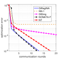
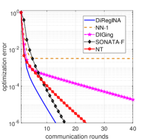
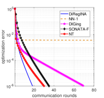
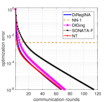
Figure 1: Distributed ridge regression: (a) star-topology; and Erdős-Rényi graph with (b) $\rho=0.20$, (c) $\rho=0.41$, (d) $\rho=0.69$.

5 Experiments

In this section we test numerically our theoretical findings on two classes of problems over meshed networks: 1) ridge regression and 2) logistic regression. Other experiments can be found in the supplementary material (cf.  Sec. A).

The network graph is generated using an Erdős-Rényi model $G(m,p)$, with $m=30$ nodes and different values of $p$ to span different level of connectivity.

We compare DiRegINA with the following methods: $\bullet$ Distributed (first-order) method with gradient tracking: we consider SONATA (Sun et al., 2019) and DIGing (Nedic et al., 2017); both build on the idea of gradient tracking, with the former applicable also to constrained problems. For the SONATA algorithm, we will simulate two instances, namely: SONATA-L (L stands for linearization) and SONATA-F (F stands for full); the former uses only first-order information in the agents’ local updates (as DGing) while the latter exploits functions’ similarity by employing local mirror-descent-based optimization. $\bullet$ Distributed accelerated first-order methods: we consider APAPC (Kovalev et al., 2020) and SSDA (Scaman et al., 2017), which employ Nesterov acceleration on the local optimization steps–with the former using primal gradients while the latter requiring gradients of the conjugate functions–and Chebyshev acceleration on the consensus steps. These schemes do not leverage any similarity among the local agents’ functions. $\bullet$ Distributed second-order methods: We implement i) Network Newton-K (NN-K) (Mokhtari et al., 2016b) with $K=1$ so that it has the same communication cost per iteration of DiRegINA ; ii) SONATA-F (Sun et al., 2019), which is a mirror descent-type distributed scheme wherein agents need to solve exactly a strongly convex optimization problem; and iii) Newton Tracking (NT) (Jiaojiao et al., 2020), which has been shown the outperform the majority of distributed second-order methods.

All the algorithms are coded in MATLAB R2019a, running on a computer with Intel(R) Core(TM) i7-8650U CPU@1.90GHz, 16.0 GB of RAM, and 64-bit Windows 10.

5.1 Distributed Ridge Regression

We train ridge regression, LIBSVM, scaled mg dataset (Flake & Lawrence, 2002), which is an instance of (P) with $f_{i}(x)=(1/2n)\left\lVert A_{i}x-b_{i}\right\rVert^{2}+\frac{\lambda}{2}\left\lVert x\right\rVert^{2}$ and $\mathcal{K}=\mathbb{R}^{d}$, with $d=6$. We set $\lambda=1/\sqrt{N}=0.0269$; we estimate $\beta=0.1457$ and $\mu=0.0929$. The graph parameter $p=0.6,0.33,0.28$, resulting in the connectivity values $\rho\approx 0.20,0.41,0.70$, respectively. We compared DiRegINA, NN-1, DIGing, SONATA-F and NT, all initialized from the same identical random point. The coefficients of the matrix $\overline{W}$ are chosen according to the Metropolis–Hastings rule (Xiao et al., 2007). The free parameters of the algorithm are tuned manually; specifically: DiRegINA, $\tau=2\beta$, $M=1e-3$, and $K=1$; NN-1, $\alpha=1e-3$ and $\epsilon=1$; DIGing, stepsize equal to $0.5$; SONATA-F, $\tau=0.27$; NT, $\epsilon=0.08$ and $\alpha=0.1$. This tuning corresponds to the best practical performance we observed.

In Fig. 1, we plot the function residual $p^{\nu}$ defined in (9) versus the communication rounds in the four aforementioned network settings. DiRegINA demonstrates good performance over first-order methods, and compares favorably also with SONATA-F (which has higher computational cost). Note the change of rate, as predicted by our theory, with linear rate in the last stage. NN-1 is not competitive while NT in some settings is comparable with DiRegINA , but we observed to be more sensitive to the tuning.

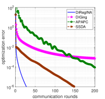
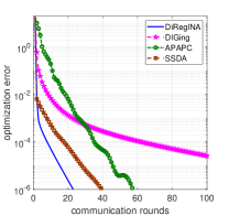
Figure 2: Distributed ridge regression. Synthetic data on Erdős-Rényi graph with $\rho=0.7$: a) $\beta/\mu=158.1$, $\sqrt{\kappa}=34.55$; b) $\beta/\mu=11.974$, $\sqrt{\kappa}=11.1$.

The second experiment aims at comparing DiRegINA with the distributed accelerated methods APAPC (Kovalev et al., 2020) and SSDA (Scaman et al., 2017) (DIGing is used as benchmark of first-order non-accelerated schemes). We tested these schemes on two instances of the Ridge regression problem using synthetic data, corresponding to $\beta/\mu\gg\sqrt{\kappa}$ and $\beta/\mu\approx\sqrt{\kappa}$. Recall that SSDA and APAPC converge linearly at a rate proportional to $\sqrt{\kappa}$ while the convergence rate of DiRegINA depends (up to log factors) on $\beta/\mu$. The problem data are generated as follows: the ground truth $x^{\ast}\in\mathbb{R}^{d}$ is a random vector, $x^{\ast}\sim\mathcal{N}(\mathbf{0},I)$, with $d=40$; samples $b_{i}\triangleq(b_{i}^{(j)})_{j=1}^{n}$, with $n=50$, are generated according to the linear model $b_{i}^{(j)}=a_{i}^{(j)\top}x^{*}+\epsilon_{i}^{(j)}$ where $\epsilon_{i}^{(j)}\sim\mathcal{N}(0,1e-4)$. To obtain controlled values for $\beta$, $A_{i}\triangleq(a_{i}^{(j)})_{j=1}^{n}$ are constructed as follows: we first generate $n$ i.i.d samples $A_{1}\triangleq(a_{1}^{(j)})_{j=1}^{n}$, with rows drawn from $\mathcal{N}(\mathbf{0},I)$; then, we set each $A_{i}=A_{1}+E_{k}$, where $E_{k}$ in a random matrix with rows drawn from $\mathcal{N}(\mathbf{0},\sigma I)$. The choices of $\sigma$ are considered resulting in two different values of $\beta$, namely: $\sigma=1/(dn)$ and $\sigma=7.5/(dn)$, resulting in $\beta=0.31$ and $\beta=4.08$, respectively. The values of the condition number read $\kappa=123.21$ and $\kappa=1.19e3$, respectively. The network is simulated as the Erdős-Rényi graph with $p=0.28$, resulting in $\rho\approx 0.7$; the number of agents is $m=30$. The tuning of DiRegINA and DIGing is the same as in Fig. 1 while APAPC and SSDA are manually tuned for best practical performance.

In Fig. 2, we plot the function residual $p^{\nu}$ defined in (9) versus the communication rounds; the two panels refer to two different values of $(\beta/\mu,\sqrt{\kappa})$. The figures show that even when $\beta/\mu$ is larger than $\sqrt{\kappa}$, DiRegINA outperforms the accelerated first order methods; roughly, it is from two to five time faster than the best simulated first order method.

Figure 3: Distributed logistic regression: 1) a4a dataset on Erdős-Rényi graph with (a) $\rho=0.367$ (b) $\rho=0.757$; 2) Synthetic data on Erdős-Rényi graph with (c) $\rho=0.367$ (d) $\rho=0.757$.

5.2 Distributed Logistic Regression

We train logistic regression models, regularized by the $\ell_{2}$-ball constraint (with radius 1). The problem is an instance of (P), with each $f_{i}(x)=-(1/n)\sum_{j=1}^{n}[\xi_{i}^{(j)}\ln(z_{i}^{(j)})+(1-\xi_{i}^{(j)})\ln(1-z_{i}^{(j)})]$, where $z_{i}^{(j)}\triangleq 1/(1+e^{-\langle a_{i}^{(j)},x\rangle})$ and binary class labels $\xi_{i}^{(j)}\in\{0,1\}$ and vectors $a_{i}^{(j)}$, $i=1,\ldots m$ and $j=1,\ldots,n$ are determined by the data set. We considered the LIBSVM a4a ($N=4,781$, $d=123$) and synthetic data ($N=900$, $d=150$). The latter are generated as follows: a random ground truth $x^{\ast}\sim\mathcal{N}(\mathbf{0},I)$, i.i.d. sample $\{a_{i}^{(j)}\}_{i,j}$, and $\{\xi_{i}^{(j)}\}_{i,j}$ are generated according to the binary model $\xi_{i}^{(j)}=1$ if $\langle a_{i}^{(j)},x^{*}\rangle\geq 0$ and $\xi_{i}^{(j)}=0$ otherwise. We consider Erdős-Rényi network models with connectivity $\rho=0.367$ and $\rho=0.757$.

We compare DiRegINA with SONATA-F and SONATA-L, since they are the only two algorithms in the list that can handle constrained problems. We report results obtained under the following tuning: (i) both SONATA variants, $\alpha=0.1$; and (ii) DiRegINA , $M=1$ and $\tau_{i}=1e-3$. The coefficients of the matrix $\overline{W}$ are chosen according to the Metropolis–Hastings rule (Xiao et al., 2007).

In Fig. 1.1, we plot the function residual $p^{\nu}$ defined in (9) versus the communication rounds, in the different mentioned network settings. On real data [panels (a)-(b)], DiRegINA and SONATA-F performs equally well, outperforming SONATA-L (first-order method). When tested on the synthetic problem [panel (c)-(d)] with less local samples $n$ and larger dimension $d$, DiRegINA shows a consistently faster rate, while SONATA-F slows down on less connected networks. Notice also the two-phase rate of DiRegINA , as predicted by our theory: an initial superlinear rate up to (approximately) the statistical precision, followed by a linear one for high accuracy.

6 Conclusions

We proposed the first second-order distributed algorithm for convex and strongly convex problems over meshed networks with global communication complexity bounds which, up to the network dependent factor $\widetilde{\mathcal{O}}(1/\sqrt{1-\rho})$, (almost) match the iteration complexity of centralized second-order method (Nesterov & Polyak, 2006) in the regime when the desired accuracy is moderate. We showed that this regime is reasonable when one considers ERM problems for which there is no need to optimize beyond the statistical error. Importantly, our method avoids expensive communications of Hessians over the network and keeps the amount of information sent in each communication round similar to first-order methods.

This paper is just a starting point towards a theory of second-order methods with performance guarantees on meshed networks under statistical similarity; many questions remain open. An obvious one is incorporating acceleration to improve communication complexity bounds under statistical similarity. A first attempt towards this goal is the follow-up work (Agafonov et al., 2021), where an accelerated second-order method exploiting statistical similarity has been analyzed for master/workers architectures. The extension to arbitrary graphs remains an open problem. Second, our main goal here has been decreasing communications, which does not guarantee optimal oracle (computational) complexity–this is because we did not take advantage of the finite-sum structure of the local optimization problems. Stochastic optimization algorithms equipped with Variance Reduction (VR) techniques have been proved to be quite effective to obtain cheaper iterations while preserving fast convergence (Johnson & Zhang, 2013; Hendrikx et al., 2020a). However, these methods do not exploit any statistical similarity, resulting in less favorable communication complexity whenever $\beta/\mu\ll Q/\mu$. It would be then interesting to investigate whether VR techniques can improve both communication and oracle complexity when statistical similarity is explicitly employed in the algorithmic design.

Acknowledgements

The work of A. Daneshmand and G. Scutari was supported by the USA NSF Grant CIF 1719205, the ARO Grant No. W911NF1810238, and the ONR Grant No. 1317827. The work of P. Dvurechensky and A. Gasnikov was prepared within the framework of the HSE University Basic Research Program and is supported by the Ministry of Science and Higher Education of the Russian Federation (Goszadaniye) No. 075-00337-20-03, project No. 0714-2020-0005.

Supplementary Material

This supplementary material is organized as follows. Sec. A provides additional numerical experiments, complementing those in Sec. 5 of the main paper. In Sec. C, we establish asymptotic convergence of DiRegINA and prove some intermediate results that are instrumental for our rate analysis. Sec. D-G are devoted to prove Sec. 4 of the paper, namely: Theorem 7 is proved in Sec. D; Theorem 9 and Corollary 11 are proved in Sec. E; and finally, Theorem 12 is proved in Sec. F.

Furthermore, there are some convergence results stated in Table 1.1 that could not be stated in the paper because of space limit; they are reported here in the following sections: i) the case of quadratic functions $f_{i}$ in the setting of Theorem 9 is stated in Theorem 18 in Sec. E.4 while the case of quadratic $f_{i}$’s in the setting of Theorem 12 is stated in Theorem 19, Sec. G.

Appendix A Additional Numerical Experiments

Convex (non-strongly convex) objective

We consider a (non-strongly) convex instance of the regression problem. Specifically, we have: $f_{i}(x)=(1/2n)\left\lVert A_{i}x-b_{i}\right\rVert^{2}$ and $\mathcal{K}=\mathbb{R}^{d}$, where $A_{i}$ and $b_{i}$ are determined by the scaled LIBSVM dataset space-ga ($N=3107$, $d=6$, and $\beta=0.6353$). The network is simulated as the Erdős-Rényi network model, with $m=30$ and two connectivity values, $\rho=0.3843$ and $\rho=0.8032$. We compared DiRegINA with the algorithms described in Sec. 4, namely: NN-1, NT, DIGing and SONATA-F. Note that NN-1 and NT are not guaranteed to converge when applied to convex (non-strongly convex) functions. The tuning of the algorithm is the same as the one described in Sec. 5.1. In Fig. 1.1, we plot the optimization error versus the communication rounds achieved by the aforementioned algorithms in the two network settings, $\rho=0.3843$ and $\rho=0.8032$. As already observed for the other simulated problems (cf. Sec. 5.1), SONATA-F shows similar performance of DiRegINA when running on well-connected networks while its performance deteriorates in poorly connected network. NT seems to be non-convergent while NN1 and DIGing converge, yet slow, to acceptable accuracy.

Figure 4: Distributed ridge regression on space-ga dataset and Erdős-Rényi graph with (a) $\rho=0.3843$ (b) $\rho=0.8032$.

$O(1/\sqrt{mn})$-regularized logistic regression

We train logistic regression models, regularized by an additive $\ell_{2}$-norm (with coefficient $\lambda>0$). The problem is an instance of (P), with each $f_{i}(x)=-(1/n)\sum_{j=1}^{n}[\xi_{i}^{(j)}\ln(z_{i}^{(j)})+(1-\xi_{i}^{(j)})\ln(1-z_{i}^{(j)})]+(\lambda/2)||x||^{2}$ and $\mathcal{K}=\mathbb{R}^{d}$, where $z_{i}^{(j)}\triangleq 1/(1+e^{-\langle a_{i}^{(j)},x\rangle})$ and binary class labels $\xi_{i}^{(j)}\in\{0,1\}$ and vectors $a_{i}^{(j)}$, $i=1,\ldots m$ and $j=1,\ldots,n$ are determined by the data set. We considered the LIBSVM a4a ($N=4,781$, $d=123$) and we set $\lambda=1/\sqrt{mn}$. The Network is simulated according to the Erdős-Rényi model with $m=30$ and connectivity $\rho=0.3372$ and $\rho=0.7387$.

We compare DiRegINA , NN-1, DIGing, SONATA-F and NT, all initialized from the same random point. The free parameters of the algorithms are tuned manually; the best practical performance are observed with the following tuning: DiRegINA is tuned as described in Sec. 5.2, i.e., $\tau=1$, $M=1e-3$, and $K=1$; NN-1, $\alpha=1e-3$ and $\epsilon=1$; DIGing, stepsize equal to $1$; SONATA-F, $\tau=0.1$; NT, $\epsilon=0.2$ and $\alpha=0.05$.

In Fig. 1.1, we plot the optimization error versus the communication rounds achieved by the aforementioned algorithms in two network settings corresponding to $\rho=0.3372$ and $\rho=0.7387$. In both settings (panels (a)-(b)), NN-1 and DIGing still exhibits slow convergence, with a slight advantage of DIGing over NN-1. DiRegINA , NT and SONATA-F, perform similarly, with DiRegINA showing some improvements when the network is better connected [panel (a)].

Figure 5: Distributed logistic regression on a4a dataset and Erdős-Rényi graph with (a) $\rho=0.3372$ (b) $\rho=0.7387$.

Appendix B Notations and Preliminary Results

We begin introducing some notation which will be used in all the proofs, along with some preliminary results.

Define

$$\delta_{i}^{\nu}\triangleq s_{i}^{\nu}-\nabla F(x_{i}^{\nu})\quad\text{and}\quad B_{i}^{\nu}\triangleq\nabla^{2}f_{i}(x_{i}^{\nu})-\nabla^{2}F(x_{i}^{\nu}),$$ (17)

The local surrogate function $\widetilde{F}_{i}(y;x_{i}^{\nu})$ in (7a) can be rewritten as

$$\widetilde{F}_{i}(y;x_{i}^{\nu})\triangleq F(x_{i}^{\nu})+\left\langle\nabla F(x_{i}^{\nu})+\delta_{i}^{\nu},y-x_{i}^{\nu}\right\rangle+\frac{1}{2}\left\langle\left[\nabla^{2}F(x_{i}^{\nu})+B_{i}^{\nu}+\tau_{i}I\right](y-x_{i}^{\nu}),y-x_{i}^{\nu}\right\rangle+\frac{M_{i}}{6}\left\lVert y-x_{i}^{\nu}\right\rVert^{3}.$$ (18)

Let us recall the following basic result, which is a consequence of Assumption 3.

Lemma 1 (Nesterov (2018, Lemma 1.2.4)).

Let $F:\mathbb{R}^{d}\rightarrow\mathbb{R}$ be a twice-differentiable function satisfying Assumption 3. Then, for all $x,y\in\mathbb{R}^{d}$,

$$\big{|}F(y)-F(x)-\left\langle\nabla F(x),y-x\right\rangle-\frac{1}{2}\left\langle\nabla^{2}F(x)(y-x),y-x\right\rangle\big{|}\leq\frac{L}{6}\left\lVert y-x\right\rVert^{3}.$$ (19)

$$\left\lVert\nabla F(y)-\nabla F(x)-\nabla^{2}F(x)(y-x)\right\rVert\leq\frac{L}{2}\left\lVert y-x\right\rVert^{2}.$$ (20)

Setting $x=x_{i}^{\nu}$ in (19) implies

$$F(x_{i}^{\nu})+\left\langle\nabla F(x_{i}^{\nu}),y-x_{i}^{\nu}\right\rangle+\frac{1}{2}\left\langle\nabla^{2}F(x_{i}^{\nu})(y-x_{i}^{\nu}),y-x_{i}^{\nu}\right\rangle\leq F(y)+\frac{L}{6}\left\lVert y-x_{i}^{\nu}\right\rVert^{3},\quad\forall y\in\mathbb{R}^{d},$$

which, together with (18), gives the following upper bound for the surrogate function $\widetilde{F}_{i}$ defined in (18):

$$\widetilde{F}_{i}(y;x_{i}^{\nu})\leq F(y)+\frac{1}{2}\left\lVert y-x_{i}^{\nu}\right\rVert^{2}_{(\beta+\tau_{i})I}+\frac{M_{i}+L}{6}\left\lVert y-x_{i}^{\nu}\right\rVert^{3}+\left\langle\delta_{i}^{\nu},y-x_{i}^{\nu}\right\rangle,\quad\forall y\in\mathbb{R}^{d},$$ (21)

where for a positive semidefinite matrix $A$, $\|x\|_{A}^{2}\triangleq\langle Ax,x\rangle$. We also denote

$$\Delta x_{i}^{\nu}\triangleq x_{i}^{\nu+}-x_{i}^{\nu},\quad\delta^{\nu}\triangleq(\delta_{i}^{\nu})_{i=1}^{m},\quad J\triangleq 11^{\top}/m,$$ (22)

where we remind that $x_{i}^{\nu+}$ is obtained by the minimization of the local surrogate function $\widetilde{F}_{i}(y;x_{i}^{\nu})$. The rest of the symbols and notations are as defined in the main manuscript.

Appendix C Asymptotic convergence of DiRegINA

In this section we prove the following theorem stating asymptotic convergence of DiRegINA .

Theorem 13.

Let Assumptions 1 and 3-5 hold, $M_{i}\geq L$ and $\tau_{i}=2\beta$ for all $i=1,\ldots,m$. If a reference matrix $\overline{W}$ satisfying Assumption 6 is used in steps (7b)-(7c), with $\rho\triangleq\lambda_{\max}(\overline{W}-{J})<1$ and $K=\widetilde{\mathcal{O}}(1/\sqrt{1-\rho})$ (explicit condition is provided in eq. (41)), then $p^{\nu}\rightarrow 0$ and $||x_{i}^{\nu}-x_{j}^{\nu}||\rightarrow 0$, as $\nu\rightarrow\infty$ for all $i,j=1,\ldots,m$.

We prove the theorem in three main steps:

• Step 1 (Sec. C.1): Deriving optimization bounds on the per-iteration decrease of $p^{\nu}$;

• Step 2 (Sec. C.2): Bounding the gradient tracking error $\delta^{\nu}$, which in turn affects the per-iteration decrease of $p^{\nu}$;

• Step 3 (Sec. C.3): Constructing a proper Lyapunov function based on the error terms in the previous two steps, whose dynamics imply asymptotic convergence of DiRegINA .

To simplify the derivations, we study the case of strongly convex or nonstronlgy convex $F$ together, by setting $\mu=0$ in the latter case.

C.1 Optimization error bounds

In this subsection we establish an upper bound for $p^{\nu+1}-p^{\nu}$ [cf. (32)]. We begin with two technical intermediate results–Lemma 2 and Lemma 3.

Lemma 2.

Under Assumption 1, there holds

$$\widetilde{F}_{i}(x_{i}^{\nu+};x_{i}^{\nu})\leq \;\widetilde{F}_{i}(x_{i}^{\nu};x_{i}^{\nu})-\frac{M_{i}}{3}\left\lVert\Delta x_{i}^{\nu}\right\rVert^{3}-\frac{\mu_{i}+\tau_{i}}{2}\left\lVert\Delta x_{i}^{\nu}\right\rVert^{2}.$$ (23)

Proof.

By the optimality of $x_{i}^{\nu+}$ in (18), we infer

$$\left\langle s_{i}^{\nu}+\left[\nabla^{2}f_{i}(x_{i}^{\nu})+\tau_{i}I\right]\Delta x_{i}^{\nu},\Delta x_{i}^{\nu}\right\rangle\leq-\frac{M_{i}}{2}\left\lVert\Delta x_{i}^{\nu}\right\rVert^{3}.$$ (24)

Since $\widetilde{F}_{i}(x_{i}^{\nu};x_{i}^{\nu})=F(x_{i}^{\nu})$, we have

$$\widetilde{F}_{i}(x_{i}^{\nu+};x_{i}^{\nu})-\widetilde{F}_{i}(x_{i}^{\nu};x_{i}^{\nu})$$

$$\overset{\eqref{tF_i_rewrite}}{=} \left\langle s_{i}^{\nu},x_{i}^{\nu+}-x_{i}^{\nu}\right\rangle+\frac{1}{2}\left\langle\left[\nabla^{2}f_{i}(x_{i}^{\nu})+\tau_{i}I\right]\Delta x_{i}^{\nu},\Delta x_{i}^{\nu}\right\rangle+\frac{M_{i}}{6}\left\lVert x_{i}^{\nu+}-x_{i}^{\nu}\right\rVert^{3}$$

$$\overset{\eqref{x_hat_opt_cubic}}{\leq} -\frac{1}{2}\left\langle\left[\nabla^{2}f_{i}(x_{i}^{\nu})+\tau_{i}I\right]\Delta x_{i}^{\nu},\Delta x_{i}^{\nu}\right\rangle-\frac{M_{i}}{3}\left\lVert\Delta x_{i}^{\nu}\right\rVert^{3}$$

$${\leq} -\frac{M_{i}}{3}\left\lVert x_{i}^{\nu+}-x_{i}^{\nu}\right\rVert^{3}-\frac{\mu_{i}+\tau_{i}}{2}\left\lVert x_{i}^{\nu+}-x_{i}^{\nu}\right\rVert^{2}.$$

∎

Lemma 3.

Let Assumptions 1 and 3-4 hold. Then, any arbitrary $\epsilon>0$, we have

$$F(x_{i}^{\nu+})-\widetilde{F}_{i}(x_{i}^{\nu+};x_{i}^{\nu})\leq -\frac{M_{i}-L}{6}||\Delta x_{i}^{\nu}||^{3}-\frac{\tau_{i}-\beta-\epsilon}{2}||\Delta x_{i}^{\nu}||^{2}+\frac{1}{2\epsilon}\left\lVert\delta_{i}^{\nu}\right\rVert^{2}.$$ (25)

Proof.

Taylor’s theorem applied to functions $\widetilde{F}_{i}(\cdot;x_{i}^{\nu})$ and $F(\cdot)$ around $x_{i}^{\nu}$ yields

$$F(x_{i}^{\nu+})= F(x_{i}^{\nu})+\left\langle\nabla F(x_{i}^{\nu}),\Delta x_{i}^{\nu}\right\rangle+\Delta x_{i}^{\nu\top}{H}_{i}^{\nu}\Delta x_{i}^{\nu},$$ (26a)

$$\widetilde{F}_{i}(x_{i}^{\nu+};x_{i}^{\nu})= \widetilde{F}_{i}(x_{i}^{\nu};x_{i}^{\nu})+\left\langle\nabla\widetilde{F}_{i}(x_{i}^{\nu};x_{i}^{\nu}),\Delta x_{i}^{\nu}\right\rangle+\Delta x_{i}^{\nu\top}\widetilde{{H}}_{i}^{\nu}\Delta x_{i}^{\nu},$$ (26b)

where

$${H}_{i}^{\nu}= \int_{0}^{1}(1-\theta)\nabla^{2}F(\theta x_{i}^{\nu+}+(1-\theta)x_{i}^{\nu})d\theta,$$

$$\widetilde{{H}}_{i}^{\nu}= \int_{0}^{1}(1-\theta)\nabla^{2}\widetilde{F}_{i}(\theta x_{i}^{\nu+}+(1-\theta)x_{i}^{\nu};x_{i}^{\nu})d\theta.$$

Since $\widetilde{F}_{i}(x_{i}^{\nu};x_{i}^{\nu})=F(x_{i}^{\nu})$ and $\nabla\widetilde{F}_{i}(x_{i}^{\nu};x_{i}^{\nu})=\nabla F(x_{i}^{\nu})+\delta_{i}^{\nu}$, subtracting (26a)-(26b) gives

$$F(x_{i}^{\nu+})-\widetilde{F}_{i}(x_{i}^{\nu+};x_{i}^{\nu})= \big{\langle}\big{(}{H}_{i}^{\nu}-\widetilde{{H}}_{i}^{\nu}\big{)}\Delta x_{i}^{\nu},\Delta x_{i}^{\nu}\big{\rangle}-\left\langle\delta_{i}^{\nu},\Delta x_{i}^{\nu}\right\rangle.$$ (27)

Now let us simplify (27). Note that the hessian of $\widetilde{F}_{i}(\cdot;x_{i}^{\nu})$ is

$$\nabla^{2}\widetilde{F}_{i}(x_{i};x_{i}^{\nu})=\nabla^{2}F(x_{i}^{\nu})+B_{i}^{\nu}+\tau_{i}I+M_{i}G(x_{i};x_{i}^{\nu}),$$ (28)

where

$$G\left(x_{i};x_{i}^{\nu}\right)\triangleq\frac{1}{2}\left(\left\lVert x_{i}-x_{i}^{\nu}\right\rVert I+\frac{(x_{i}-x_{i}^{\nu})(x_{i}-x_{i}^{\nu})^{\top}}{\left\lVert x_{i}-x_{i}^{\nu}\right\rVert}\right).$$

Hence,

$$\begin{split}&{H}_{i}^{\nu}-\widetilde{{H}}_{i}^{\nu}\\ =&\int_{0}^{1}(1-\theta)\nabla^{2}F\left(\theta x_{i}^{\nu+}+(1-\theta)x_{i}^{\nu}\right)d\theta-\int_{0}^{1}(1-\theta)\nabla^{2}\widetilde{F}_{i}\left(\theta x_{i}^{\nu+}+(1-\theta)x_{i}^{\nu};x_{i}^{\nu}\right)d\theta\\ \overset{\eqref{nabla2Ftilde_hessian}}{=}&\int_{0}^{1}(1-\theta)\nabla^{2}F\left(\theta x_{i}^{\nu+}+(1-\theta)x_{i}^{\nu}\right)d\theta-\int_{0}^{1}(1-\theta)\left[\nabla^{2}F(x_{i}^{\nu})+B_{i}^{\nu}\right]d\theta-\int_{0}^{1}(1-\theta)\tau_{i}Id\theta\\ &-\int_{0}^{1}(1-\theta)M_{i}\theta G(x_{i}^{\nu+};x_{i}^{\nu})d\theta\\ =&\int_{0}^{1}(1-\theta)\left(\nabla^{2}F\left(\theta x_{i}^{\nu+}+(1-\theta)x_{i}^{\nu}\right)-\nabla^{2}F(x_{i}^{\nu})\right)d\theta\\ &-\int_{0}^{1}(1-\theta)B_{i}^{\nu}d\theta-\int_{0}^{1}(1-\theta)\tau_{i}Id\theta-\int_{0}^{1}(1-\theta)M_{i}\theta G(x_{i}^{\nu+};x_{i}^{\nu})d\theta\\ \overset{{\rm(a)}}{\preceq}&\int_{0}^{1}(1-\theta)L\theta||x_{i}^{\nu+}-x_{i}^{\nu}||Id\theta\\ &-\int_{0}^{1}(1-\theta)B_{i}^{\nu}d\theta-\int_{0}^{1}(1-\theta)\tau_{i}Id\theta-\int_{0}^{1}(1-\theta)M_{i}\theta G(x_{i}^{\nu+};x_{i}^{\nu})d\theta\\ =&-\frac{M_{i}}{6}G(x_{i}^{\nu+};x_{i}^{\nu})+\frac{L}{6}||x_{i}^{\nu+}-x_{i}^{\nu}||I-\frac{\tau_{i}}{2}I-\frac{B_{i}^{\nu}}{2}\end{split}$$ (29)

where (a) holds since $\nabla^{2}F$ is $L$-Lipschitz continuous. Combining (27) and (29), we conclude

$$F(x_{i}^{\nu+})-\widetilde{F}_{i}(x_{i}^{\nu+};x_{i}^{\nu})\leq -\frac{M_{i}-L}{6}||\Delta x_{i}^{\nu}||^{3}-\frac{\tau_{i}}{2}||\Delta x_{i}^{\nu}||^{2}-\frac{1}{2}\left\langle B_{i}^{\nu}\Delta x_{i}^{\nu},\Delta x_{i}^{\nu}\right\rangle-\left\langle\delta_{i}^{\nu},\Delta x_{i}^{\nu}\right\rangle$$

$$\leq -\frac{M_{i}-L}{6}||\Delta x_{i}^{\nu}||^{3}-\frac{\tau_{i}-\beta-\epsilon}{2}||\Delta x_{i}^{\nu}||^{2}+\frac{1}{2\epsilon}\left\lVert\delta_{i}^{\nu}\right\rVert^{2},$$

for arbitrary $\epsilon>0$, where the last inequality is due to the Cauchy-Schwarz inequality and $|\left\langle B_{i}^{\nu}\Delta x_{i}^{\nu},\Delta x_{i}^{\nu}\right\rangle|\leq\beta||\Delta x_{i}^{\nu}||^{2}$, which is a consequence of (17) and Assumption 4. ∎

We are now in a position to prove the main result of this subsection.

Combining (23) in Lemma 3 with (25) in Lemma 2, and using $\widetilde{F}_{i}(x_{i}^{\nu};x_{i}^{\nu})=F(x_{i}^{\nu})$, yields

$$F(x_{i}^{\nu+})-F(x_{i}^{\nu})\leq -\left(\frac{M_{i}}{2}-\frac{L}{6}\right)||\Delta x_{i}^{\nu}||^{3}-\left(\frac{\mu_{i}}{2}+\tau_{i}-\frac{\beta+\epsilon}{2}\right)||\Delta x_{i}^{\nu}||^{2}+\frac{1}{2\epsilon}\left\lVert\delta_{i}^{\nu}\right\rVert^{2}.$$

Since under either Assumption 1 or Assumption 2 combined with Assumption 4 it holds that $\mu_{i}\geq\max\left\{0,\mu-\beta\right\}$, we obtain

$$F(x_{i}^{\nu+})-F(x_{i}^{\nu})\leq -\left(\frac{M_{i}}{2}-\frac{L}{6}\right)||\Delta x_{i}^{\nu}||^{3}-\left(\frac{\max(0,\mu-\beta)}{2}+\tau_{i}-\frac{\beta+\epsilon}{2}\right)||\Delta x_{i}^{\nu}||^{2}+\frac{1}{2\epsilon}\left\lVert\delta_{i}^{\nu}\right\rVert^{2}.$$ (30)

Denoting $p^{\nu+}\triangleq(1/m)\sum_{i=1}^{m}\left\{F(x_{i}^{\nu+})-F(\widehat{x})\right\}$, we derive a simple relation with $p^{\nu+1}$:

$$p^{\nu+1}+F(\widehat{x}) =\frac{1}{m}\sum_{i=1}^{m}F\Big{(}x^{\nu+1}_{i}\Big{)}\overset{\eqref{DiRegINA_pseudocode}}{=}\frac{1}{m}\sum_{i=1}^{m}F\Big{(}\sum_{j=1}^{m}(W_{K})_{i,j}\,x_{j}^{\nu+}\Big{)}$$ (31)

$$\overset{(a)}{\leq}\frac{1}{m}\sum_{i,j=1}^{m}(W_{K})_{i,j}F\Big{(}x^{\nu+}_{j}\Big{)}\overset{(b)}{=}\frac{1}{m}\sum_{j=1}^{m}F\Big{(}x^{\nu+}_{j}\Big{)}=p^{\nu+}+F(\widehat{x}),$$

where (a) is due to convexity of $F$ (cf. Assumptions 1 and 2) and $\sum_{j=1}^{m}(W_{K})_{ij}=1$ (cf. Assumption 6); and in (b) we used $\sum_{i=1}^{m}(W_{K})_{ij}=1$ (cf. Assumption 6). Summing (30) over $i$ while setting $\epsilon=\beta$, $\tau_{i}=2\beta$ and $M_{i}\geq L/3$ (recall that it is assumed $M_{i}\geq L$), gives the desired per-iteration decrease of $p^{\nu}$ when $\left\lVert\delta^{\nu}\right\rVert$ is sufficiently small:

$$p^{\nu+1}-p^{\nu}\overset{\eqref{pnuplus_pnu}}{\leq}p^{\nu+}-p^{\nu}\leq -\frac{\max(\mu,\beta)}{2}\cdot\frac{1}{m}\sum_{i=1}^{m}\|\Delta x_{i}^{\nu}\|^{2}+\frac{1}{2m\beta}\left\lVert\delta^{\nu}\right\rVert^{2}.$$ (32)

C.2 Network error bounds

The goal of this subsection is to prove an upper bound for $\left\lVert\delta^{\nu}\right\rVert$ in terms of the number of communication steps $K$, implying that this error can be made sufficiently small by choosing sufficiently large $K$. For notation simplicity and without loss of generality, we assume $d=1$; the case $d>1$ follows trivially.

Recall that $x^{\nu}\triangleq(x_{i}^{\nu})_{i=1}^{m}$, $s^{\nu}\triangleq(s_{i}^{\nu})_{i=1}^{m}$, ${J}\triangleq(1/m)1_{m}1_{m}^{\top}$, and

$$x_{\bot}^{\nu}\triangleq(I-{J})x^{\nu}=x^{\nu}-1_{m}\frac{1_{m}^{\top}x^{\nu}}{m},\quad s_{\bot}^{\nu}\triangleq(I-{J})s^{\nu}=s^{\nu}-1_{m}\frac{1_{m}^{\top}s^{\nu}}{m},\quad\Delta x^{\nu}\triangleq(\Delta x_{i}^{\nu})_{i=1}^{m}.$$

Note that the vectors $x_{\bot}^{\nu}$ and $s_{\bot}^{\nu}$ are the consensus and gradient-tracking errors; when $\|x_{\bot}^{\nu}\|=\|s_{\bot}^{\nu}\|=0$, we have $x_{i}^{\nu}=x_{j}^{\nu}$ and $s^{\nu}_{i}=s^{\nu}_{j}$ for all $i,j=1,\ldots,m$. The following holds for $x_{\bot}^{\nu}$ and $s_{\bot}^{\nu}$.

Lemma 4 (Proposition 3.5 in Sun et al. (2019)).

Under Assumptions 1 and 5-6, for all $\nu\geq 0$,

$$\|x_{\bot}^{\nu+1}\| \leq\rho_{K}\|x_{\bot}^{\nu}\|+\rho_{K}\|\Delta x^{\nu}\|,$$ (33a)

$$\|s_{\bot}^{\nu+1}\| \leq\rho_{K}\|s_{\bot}^{\nu}\|+2Q_{\max}\rho_{K}\|x_{\bot}^{\nu}\|+Q_{\max}\rho_{K}\|\Delta x^{\nu}\|,$$ (33b)

where $\rho_{K}=\lambda_{\max}(W_{K}-{J})<1$. Note that in case of $K$-rounds of communications using a reference matrix $\overline{W}$ with $\rho\triangleq\lambda_{\max}(\overline{W}-{J})<1$, we have $\rho_{K}=\rho^{K}$; if Chebyshev acceleration is employed, we have $\rho_{K}=\left(1-\sqrt{1-\rho}\right)^{K}$.

Now let us bound $\delta_{i}^{\nu}$ defined in (17). Note that by column-stochasticity of ${W}_{K}$ and initialization rule $s_{i}^{0}=\nabla f_{i}(x_{i}^{0})$, it can be trivially concluded from (7c) that

$$1_{m}^{\top}s^{\nu}=\sum_{j=1}^{m}\nabla f_{j}(x_{j}^{\nu}).$$

Hence,

$$\left\lVert\delta_{i}^{\nu}\right\rVert^{2}= \Big{\|}s_{i}^{\nu}-\frac{1_{m}^{\top}s^{\nu}}{m}+\frac{1}{m}\sum_{j=1}^{m}\nabla f_{j}(x_{j}^{\nu})-\nabla F(x_{i}^{\nu})\Big{\|}^{2}$$ (34)

$$\overset{(a)}{\leq} 2\Big{\|}s_{i}^{\nu}-\frac{1_{m}^{\top}s^{\nu}}{m}\Big{\|}^{2}+\frac{2Q_{\max}^{2}}{m}\left(\sum_{j=1}^{m}\Big{\|}x_{i}^{\nu}\pm\frac{1_{m}^{\top}x^{\nu}}{m}-x_{j}^{\nu}\Big{\|}^{2}\right)$$

$$\leq 2\Big{\|}s_{i}^{\nu}-\frac{1_{m}^{\top}s^{\nu}}{m}\Big{\|}^{2}+\frac{4Q_{\max}^{2}}{m}\left(\|x_{\bot}^{\nu}\|^{2}+m~{}\Big{\|}x_{i}^{\nu}-\frac{1_{m}^{\top}x^{\nu}}{m}\Big{\|}^{2}\right),$$

where (a) is due to $Q_{\max}$-Lipschitz continuity of $\nabla f_{i}$. Summing (34) over $i$ and taking the square root, gives

$$\left\lVert\delta^{\nu}\right\rVert\leq\tilde{\delta}^{\nu}\triangleq\sqrt{2}\left(\|s_{\bot}^{\nu}\|+2Q_{\max}\|x_{\bot}^{\nu}\|\right).$$ (35)

It remains to bound $\tilde{\delta}^{\nu}$ defined above:

$$\tilde{\delta}^{\nu+1}=\sqrt{2}\left(\|s_{\bot}^{\nu+1}\|+2Q_{\max}\|x_{\bot}^{\nu+1}\|\right)\overset{(a)}{\leq} \rho_{K}\sqrt{2}\left(\|s_{\bot}^{\nu}\|+4Q_{\max}\|x_{\bot}^{\nu}\|\right)+3\sqrt{2}Q_{\max}\rho_{K}\|\Delta x^{\nu}\|$$

$$\leq 2\rho_{K}\tilde{\delta}^{\nu}+3\sqrt{2}Q_{\max}\rho_{K}\|\Delta x^{\nu}\|,$$

where in (a) we used Lemma 4 [cf. (33a)-(33b)]. Consequently,

$$(\tilde{\delta}^{\nu+1})^{2}\leq 8\rho_{K}^{2}(\tilde{\delta}^{\nu})^{2}+36Q_{\max}^{2}\rho_{K}^{2}\|\Delta x^{\nu}\|^{2}.$$ (36)

Since $\rho_{K}$ decreases as $K$ increases, the latter inequality provides a leverage to make $\tilde{\delta}^{\nu+1}$ sufficiently small by choosing $K$ sufficiently large.

C.3 Asymptotic convergence

We combine the results of the previous two subsections to finally prove Theorem 13. Combining (32) and (35), we obtain

$$p^{\nu+1}\leq \;\;p^{\nu}-\frac{\max(\beta,\mu)}{2m}\|\Delta x^{\nu}\|^{2}+\frac{1}{2m\beta}(\tilde{\delta}^{\nu})^{2}.$$ (37)

Next, we combine (36) with (37) multiplied by some weight $w>0$ to obtain

$$wp^{\nu+1}+(\tilde{\delta}^{\nu+1})^{2}\leq wp^{\nu}+\left(8\rho_{K}^{2}+\frac{w}{2m\beta}\right)(\tilde{\delta}^{\nu})^{2}-w\left(\frac{\max(\beta,\mu)}{2m}-\frac{36}{w}Q_{\max}^{2}\rho_{K}^{2}\right)||\Delta x^{\nu}||^{2}.$$ (38)

Let $w=c_{w}\beta$, for some $0<c_{w}\leq 1$. Then, if

$$8\rho_{K}^{2}+\frac{w}{2m\beta}\leq c_{w},\quad\frac{\max(\beta,\mu)}{4m}\geq\frac{36}{w}Q_{\max}^{2}\rho_{K}^{2},$$ (39)

(38) becomes

$$wp^{\nu+1}+(\tilde{\delta}^{\nu+1})^{2}\leq wp^{\nu}+c_{w}(\tilde{\delta}^{\nu})^{2}-\frac{w\max(\beta,\mu)}{4m}||\Delta x^{\nu}||^{2}.$$ (40)

Note that by Lemma 4, condition (39) holds if

$$K\geq\frac{1}{\sqrt{1-\rho}}\log\left(\max\left\{\frac{2\sqrt{2}}{\sqrt{c_{w}(1-\frac{1}{2m})}},\frac{12\sqrt{m}Q_{\max}}{\sqrt{c_{w}\beta\max(\beta,\mu)}}\right\}\right).$$ (41)

Denoting

$$\xi^{\nu}\triangleq wp^{\nu}+(\tilde{\delta}^{\nu})^{2},$$ (42)

let us show that $\xi^{\nu}\rightarrow 0$ as $\nu\to\infty$, which implies that the optimization error $p^{\nu}$ and network error $\tilde{\delta}^{\nu}$ asymptotically vanish. Since $\xi^{\nu}\geq 0$, inequality (40) implies $\sum_{\nu=0}^{\infty}||\Delta x^{\nu}||^{2}<\infty$. Thus, $||\Delta x^{\nu}||\rightarrow 0$; and $||\Delta x^{\nu}||\leq D_{1}$, for some $D_{1}>0$ and all $\nu\geq 0$. Further, $\{\xi^{\nu}\}_{\nu}$ is non-increasing and $||\xi^{\nu}||\leq D_{2}$ for some $D_{2}>0$ and all $\nu\geq 0$. Thus, $p^{\nu}\leq D_{2}/w$, which together with Assumption 1(iv) and Assumption 2, also implies $||x_{i}^{\nu}||\leq D_{3}$ for some $D_{3}$, all $i$ and $\nu\geq 0$. Using $||\Delta x^{\nu}||\rightarrow 0$ and (36), if $8\rho_{K}^{2}<1$ (which holds under (41)), we obtain that $\tilde{\delta}^{\nu}\rightarrow 0$. Finally, it remains to show that $p^{\nu}\rightarrow 0$. Using optimality condition of $x^{\nu+}_{i}$ defined in (7a), we get

$$\left\langle\nabla F(x_{i}^{\nu})+\delta_{i}^{\nu}+\left[\nabla^{2}F(x_{i}^{\nu})+B_{i}^{\nu}+\tau_{i}I\right]\Delta x_{i}^{\nu}+\frac{M_{i}}{2}||\Delta x_{i}^{\nu}||\Delta x_{i}^{\nu},\widehat{x}-x^{\nu+}_{i}\right\rangle\geq 0.$$

Rearranging terms gives

$$\left\langle\nabla F(x_{i}^{\nu})+\nabla^{2}F(x_{i}^{\nu})\Delta x_{i}^{\nu},\widehat{x}-x^{\nu+}_{i}\right\rangle$$ (43)

$$\geq \Big{\langle}\frac{M_{i}}{2}||\Delta x_{i}^{\nu}||\Delta x_{i}^{\nu},x^{\nu+}_{i}-\widehat{x}\Big{\rangle}+\left\langle\delta_{i}^{\nu},x^{\nu+}_{i}-\widehat{x}\right\rangle+\left\langle\tilde{B}_{i}^{\nu}\Delta x_{i}^{\nu},x^{\nu+}_{i}-\widehat{x}\right\rangle,$$

where $\tilde{B}_{i}^{\nu}\triangleq B_{i}^{\nu}+\tau_{i}I$. By convexity of $F$, we can write

$$0\geq F(\widehat{x})-F(x^{\nu+}_{i})$$ (44)

$$\geq \left\langle\nabla F(x^{\nu+}_{i}),\widehat{x}-x^{\nu+}_{i}\right\rangle$$

$$= \left\langle\nabla F(x^{\nu+}_{i})-\nabla F(x_{i}^{\nu})-\nabla^{2}F(x_{i}^{\nu})\Delta x_{i}^{\nu},\widehat{x}-x^{\nu+}_{i}\right\rangle+\left\langle\nabla F(x_{i}^{\nu})+\nabla^{2}F(x_{i}^{\nu})\Delta x_{i}^{\nu},\widehat{x}-x^{\nu+}_{i}\right\rangle$$

$$\overset{\eqref{x_hat_opt_cond}}{\geq} \left\langle\nabla F(x^{\nu+}_{i})-\nabla F(x_{i}^{\nu})-\nabla^{2}F(x_{i}^{\nu})\Delta x_{i}^{\nu},\widehat{x}-x^{\nu+}_{i}\right\rangle+\Big{\langle}\frac{M_{i}}{2}||\Delta x_{i}^{\nu}||\Delta x_{i}^{\nu},x^{\nu+}_{i}-\widehat{x}\Big{\rangle}$$

$$+\left\langle\delta_{i}^{\nu},x^{\nu+}_{i}-\widehat{x}\right\rangle+\left\langle\tilde{B}_{i}^{\nu}\Delta x_{i}^{\nu},x^{\nu+}_{i}-\widehat{x}\right\rangle.$$

Using Lipschitz continuity of $\nabla F$, $||\Delta x_{i}^{\nu}||\rightarrow 0$ and $\tilde{\delta}^{\nu}\rightarrow 0$ (hence $||\delta_{i}^{\nu}||\rightarrow 0$), we conclude that the RHS of (44) asymptotically vanishes, for all $i=1,\ldots,m$. Hence, $F(x^{\nu+}_{i})-F(\widehat{x})\rightarrow 0$, for all $i=1,\ldots,m$. Using (31), we finally obtain $p^{\nu}\rightarrow 0$.

Finally, by (35) and $\tilde{\delta}^{\nu}\rightarrow 0$, we obtain $\|s_{\bot}^{\nu}\|\to 0$ and $\|x_{\bot}^{\nu}\|\to 0$, implying $||x_{i}^{\nu}-x_{j}^{\nu}||\rightarrow 0$, for all $i,j=1,\ldots,m$ as $\nu\to\infty$. This concludes the proof of Theorem 13.

Remark 14.

Note that (36) implies

$$(\tilde{\delta}^{\nu})^{2}\leq\rho_{K}^{2}\bar{D}_{\delta},\quad\bar{D}_{\delta}\triangleq 8D_{2}+36Q_{\max}^{2}D_{1}^{2},\quad\forall\nu\geq 0,$$ (45)

since $(\tilde{\delta}^{\nu})^{2}\leq\xi^{\nu}\leq D_{2}$ and $||\Delta x^{\nu}||\leq D_{1}$, for all $\nu\geq 0$.

Appendix D Proof of Theorem 7

We first prove a detailed “region-based” complexity of DiRegINA (cf. Theorem 15, Subsec. D.1) for the prevalent scenario $0<\beta\leq 1$ [recall that typically $\beta=\mathcal{O}(1/\sqrt{n})$]. For the sake of completeness, the case $\beta\geq 1$ is studied in Theorem 16 (cf. Subsec. D.2). Building on Theorems 15-16, we can finally prove the main result, Theorem 7 (cf. Subsec. D.3).

D.1 Complexity Analysis when $0<\beta\leq 1$

Theorem 15 ($0<\beta\leq 1$ and $L>0$).

Let Assumptions 1 and 3 -5 hold along with $0<\beta\leq 1$. Let $M_{i}=L>0$, $\tau_{i}=2\beta$, and recall the definition of $D>0$ implying $||x_{i}^{0}-\widehat{x}||\leq D$, for all $i=1,\ldots,m$. W.l.o.g. assume $D\geq 2/L$. Pick an accuracy $\varepsilon>0$. If a reference matrix $\overline{W}$ satisfying Assumption 6 is used in steps (7b)-(7c), with $\rho\triangleq\lambda_{\max}(\overline{W}-{J})<1$ and $K=\widetilde{\mathcal{O}}(\log(1/\varepsilon)/\sqrt{1-\rho})$ (the explicit expression of $K$ can be found in (63)), then the sequence $\{p^{\nu}\}$ generated by DiRegINA satisfies the following:

• if $p^{\nu}\geq 2LD^{3}$,

  $$p^{\nu+1}\leq\frac{5}{6}~{}p^{\nu},$$

• if $\beta^{2}\cdot(2LD^{3})\leq p^{\nu}\leq 2LD^{3}$,

  $$p^{\nu}\leq\frac{244\cdot LD^{3}}{\nu^{2}},$$

• if $\varepsilon\leq p^{\nu}\leq\beta^{2}\cdot(2LD^{3})$,

  $$p^{\nu}\leq 24^{2}\cdot(LD^{3})^{2}\cdot\frac{\beta^{2}}{\varepsilon}\cdot\frac{1}{\nu^{2}}.$$

Proof.

Recalling Lemma 3 from the proof of Theorem 13, we can write

$$F(x_{i}^{\nu+})\leq\widetilde{F}_{i}(x_{i}^{\nu+};x_{i}^{\nu})+\frac{1}{2\epsilon}\left\lVert\delta_{i}^{\nu}\right\rVert^{2},$$ (46)

for arbitrary $\epsilon>0$, $M_{i}\geq L$, and $\tau_{i}\geq\beta+\epsilon$. In addition, by the upperbound approximation of $\widetilde{F}_{i}(\cdot;x_{i}^{\nu})$ in (21), there holds

$$\widetilde{F}_{i}(y;x_{i}^{\nu})\leq F(y)+\frac{1}{2}\left\lVert y-x_{i}^{\nu}\right\rVert^{2}_{(\beta+\tau_{i}+\epsilon)I}+\frac{M_{i}+L}{6}\left\lVert y-x_{i}^{\nu}\right\rVert^{3}+\frac{1}{2\epsilon}\left\lVert\delta_{i}^{\nu}\right\rVert^{2},\quad\forall y\in\mathcal{K}.$$ (47)

Let $\alpha_{0}\in(0,1]$. Set $\epsilon=\beta$ and $\tau_{i}=2\beta$. By (46)-(47) and $x^{\nu+}_{i}$ being the minimizer of $\widetilde{F}(\cdot;x_{i}^{\nu})$ [see (7a)], we obtain

$$F(x_{i}^{\nu+})-F(\widehat{x})$$ (48)

$$\leq \min_{y\in\mathcal{K}}\left\{F(y)-F(\widehat{x})+2\beta\left\lVert y-x_{i}^{\nu}\right\rVert^{2}+\frac{M_{i}+L}{6}\left\lVert y-x_{i}^{\nu}\right\rVert^{3}+\frac{1}{\beta}\left\lVert\delta_{i}^{\nu}\right\rVert^{2}\right\}$$

$$\leq \min_{\alpha\in[0,\alpha_{0}]}\Big{\{}F(y)-F(\widehat{x})+2\beta\left\lVert y-x_{i}^{\nu}\right\rVert^{2}+\frac{M_{i}+L}{6}\left\lVert y-x_{i}^{\nu}\right\rVert^{3}+\frac{1}{\beta}\left\lVert\delta_{i}^{\nu}\right\rVert^{2}$$

$$\qquad\qquad\qquad\qquad\qquad\qquad\qquad:y=\alpha\widehat{x}+(1-\alpha)x_{i}^{\nu}\Big{\}}$$

$$\leq \min_{\alpha\in[0,\alpha_{0}]}\Big{\{}(1-\alpha)\left(F(x_{i}^{\nu})-F(\widehat{x})\right)$$

$$\qquad\qquad+2\beta\alpha^{2}\left\lVert\widehat{x}-x_{i}^{\nu}\right\rVert^{2}+\frac{M_{i}+L}{6}\alpha^{3}\left\lVert\widehat{x}-x_{i}^{\nu}\right\rVert^{3}+\frac{1}{\beta}\left\lVert\delta_{i}^{\nu}\right\rVert^{2}\Big{\}},$$

where the last inequality holds by the convexity of $F$. Note that, by definition, $||x_{i}^{0}-\widehat{x}||\leq D,$ for all $i=1,\ldots,m$. Assuming $||x_{i}^{\nu}-\widehat{x}||\leq D$, for all $i=1,\ldots,m$, we prove descent at iteration $\nu+1$, i.e. $p^{\nu+1}<p^{\nu}$, unless $p^{\nu}=0$. Note that by Assumption 1(iv), if $\{p^{\nu}\}_{\nu}$ is non-increasing, then $||x_{i}^{\nu}-\widehat{x}||\leq D$ for all $\nu\geq 0$ and $i=1,\ldots,m$. Now set $M_{i}=L$ in (48) and compute the mean over $i=1,\ldots,m$, which yields

$$p^{\nu+1}\overset{\eqref{pnuplus_pnu}}{\leq}p^{\nu+}\leq\min_{\alpha\in[0,\alpha_{0}]}\Big{\{}(1-\alpha)p^{\nu}+2\beta\alpha^{2}D^{2}+\frac{LD^{3}}{3}\alpha^{3}+\frac{1}{m\beta}\left\lVert\delta^{\nu}\right\rVert^{2}\Big{\}}.$$ (49)

Denote

$$C_{1}\triangleq\frac{LD^{3}}{3}.$$ (50)

Since $D\geq\frac{2}{L}$, it holds $2\beta D^{2}\leq 3\beta C_{1}$. Then, setting $\alpha_{0}=\min\{1,p^{\nu}/(6\beta C_{1})\}$ in (49) yields

$$p^{\nu+1}\leq \min_{\alpha\in[0,\min\{1,\frac{p^{\nu}}{6\beta C_{1}}\}]}\Big{\{}(1-\alpha)p^{\nu}+3\beta C_{1}\alpha^{2}+C_{1}\alpha^{3}+\frac{1}{m\beta}\left\lVert\delta^{\nu}\right\rVert^{2}\Big{\}}$$ (51)

$$\leq \min_{\alpha\in[0,\min\{1,\frac{p^{\nu}}{6\beta C_{1}}\}]}\Big{\{}(1-\alpha/2)p^{\nu}+C_{1}\alpha^{3}+\frac{1}{m\beta}\left\lVert\delta^{\nu}\right\rVert^{2}\Big{\}}.$$

Let us assess (51) over the following “regions”. Denoting by $\alpha^{\ast}$ the minimizer of the optimization problem at the RHS of (51), we have the following:

(a) If $p^{\nu}\geq 6C_{1}$, then $\alpha^{\ast}=1$ and

$$p^{\nu+1}\leq\frac{1}{2}p^{\nu}+C_{1}+\frac{1}{m\beta}\left\lVert\delta^{\nu}\right\rVert^{2}\leq\left(\frac{1}{2}+\frac{1}{6}\right)p^{\nu}+\frac{1}{m\beta}\left\lVert\delta^{\nu}\right\rVert^{2},$$ (52)

and under the condition

$$\frac{1}{m\beta}\left\lVert\delta^{\nu}\right\rVert^{2}\leq\frac{1}{6}p^{\nu}\impliedby\frac{1}{m\beta}\left\lVert\delta^{\nu}\right\rVert^{2}\leq C_{1},$$ (53)

(52) yields

$$p^{\nu+1}\leq\frac{5}{6}~{}p^{\nu}.$$

Note that, by (45) and Lemma 4, condition (53) holds if

$$K\geq\frac{1}{\sqrt{1-\rho}}\cdot\frac{1}{2}\log\left(\frac{\bar{D}_{\delta}}{m\beta C_{1}}\right).$$ (54)

(b) If $6\beta^{2}C_{1}\leq p^{\nu}\leq 6C_{1}$, then $\alpha^{\ast}=\sqrt{\frac{p^{\nu}}{6C_{1}}}$ and

$$p^{\nu+1}\leq p^{\nu}-\frac{(p^{\nu})^{3/2}}{3\sqrt{6C_{1}}}+\frac{1}{m\beta}\left\lVert\delta^{\nu}\right\rVert^{2},$$ (55)

and if (similar to derivation of (54))

$$K\geq\frac{1}{\sqrt{1-\rho}}\cdot\frac{1}{2}\log\left(\frac{\bar{D}_{\delta}}{m\beta^{4}C_{1}}\right)\implies\frac{1}{m\beta}\left\lVert\delta^{\nu}\right\rVert^{2}\leq\beta^{3}C_{1}\implies\frac{1}{m\beta}\left\lVert\delta^{\nu}\right\rVert^{2}\leq\frac{(p^{\nu})^{3/2}}{6\sqrt{6C_{1}}},$$ (56)

(55) implies

$$p^{\nu+1}\leq p^{\nu}-\frac{(p^{\nu})^{3/2}}{6\sqrt{6C_{1}}}.$$ (57)

Finally, since $p^{\nu}$ is non-increasing,

$$\frac{1}{\sqrt{p^{\nu+1}}}-\frac{1}{\sqrt{p^{\nu}}}= \frac{p^{\nu}-p^{\nu+1}}{\left(\sqrt{p^{\nu}}+\sqrt{p^{\nu+1}}\right)\sqrt{p^{\nu}p^{\nu+1}}}\overset{\eqref{recursion_cvx_stage3}}{\geq}\frac{\frac{1}{6\sqrt{6C_{1}}}(p^{\nu})^{3/2}}{\left(\sqrt{p^{\nu}}+\sqrt{p^{\nu+1}}\right)\sqrt{p^{\nu}p^{\nu+1}}}$$

$$\geq c_{0}\triangleq\frac{1}{12}\sqrt{\frac{1}{6C_{1}}},$$

and consequently,

$$p^{\nu}\leq\frac{1}{c_{0}^{2}\Big{(}\nu+\frac{1}{c_{0}\sqrt{p^{0}}}\Big{)}^{2}}\leq\frac{1}{c_{0}^{2}\nu^{2}}.$$

(c) If $\varepsilon\leq p^{\nu}\leq 6\beta^{2}C_{1}$, then $\alpha^{\ast}=\frac{p^{\nu}}{6\beta C_{1}}$ and

$$p^{\nu+1}\leq p^{\nu}-\frac{(p^{\nu})^{2}}{18\beta C_{1}}+\frac{1}{m\beta}\left\lVert\delta^{\nu}\right\rVert^{2},$$ (58)

and if (similar to derivation of (54))

$$K\geq\frac{1}{\sqrt{1-\rho}}\cdot\frac{1}{2}\log\left(\frac{36C_{1}\bar{D}_{\delta}}{m\varepsilon^{2}}\right)\implies\frac{1}{m\beta}\left\lVert\delta^{\nu}\right\rVert^{2}\leq\frac{\varepsilon^{2}}{36\beta C_{1}}\implies\frac{1}{m\beta}\left\lVert\delta^{\nu}\right\rVert^{2}\leq\frac{(p^{\nu})^{2}}{36\beta C_{1}},$$ (59)

we deduce from (58)

$$p^{\nu+1}\leq p^{\nu}-\frac{(p^{\nu})^{2}}{36\beta C_{1}}.$$ (60)

Since $p^{\nu}$ is non-increasing,

$$\frac{1}{\sqrt{p^{\nu+1}}}-\frac{1}{\sqrt{p^{\nu}}}= \frac{p^{\nu}-p^{\nu+1}}{\left(\sqrt{p^{\nu}}+\sqrt{p^{\nu+1}}\right)\sqrt{p^{\nu}p^{\nu+1}}}\overset{\eqref{cvx_last_stage_bound2}}{\geq}\frac{\frac{1}{36\beta C_{1}}(p^{\nu})^{2}}{\left(\sqrt{p^{\nu}}+\sqrt{p^{\nu+1}}\right)\sqrt{p^{\nu}p^{\nu+1}}}$$ (61)

$$\geq \tilde{c}_{0}\triangleq\frac{\sqrt{\varepsilon}}{72\beta C_{1}},$$

and consequently,

$$p^{\nu}\leq\frac{1}{\tilde{c}_{0}^{2}\Big{(}\nu+\frac{1}{\tilde{c}_{0}\sqrt{p^{0}}}\Big{)}^{2}}\leq\frac{1}{\tilde{c}_{0}^{2}\nu^{2}}=72^{2}\cdot C_{1}^{2}\cdot\frac{\beta^{2}}{\varepsilon}\cdot\frac{1}{\nu^{2}}.$$ (62)

Finally, combining all the conditions (41), (54),(56), and (59), the requirement on $K$ reads

$$K\geq\frac{1}{\sqrt{1-\rho}}\cdot\frac{1}{2}\log\left(\max\left\{\frac{16}{c_{w}},\frac{12^{2}mQ_{\max}^{2}}{c_{w}\beta\max(\beta,\mu)},\frac{\bar{D}_{\delta}}{\min\left\{m\beta C_{1},m\beta^{4}C_{1},\frac{m}{36C_{1}}\varepsilon^{2}\right\}}\right\}\right),$$ (63)

where $\bar{D}_{\delta}$ and $C_{1}$ are defined in (45) and (50), respectively. ∎

D.2 Complexity Analysis when $\beta\geq 1$

Theorem 16 ($\beta\geq 1$ and $L>0$).

Let Assumptions 1 and 3-5 hold and $\beta\geq 1$. Let $M_{i}=L>0$, $\tau_{i}=2\beta$, and recall the definition of $D>0$ implying $\max_{i\in[m]}||x_{i}^{0}-\widehat{x}||\leq D$. W.l.o.g. assume $D\geq 2/L$. Pick an arbitrary $\varepsilon>0$. If a reference matrix $\overline{W}$ satisfying Assumption 6 is used in steps (7b)-(7c), with $\rho\triangleq\lambda_{\max}(\overline{W}-{J})<1$ and $K=\widetilde{\mathcal{O}}(\log(1/\varepsilon)/\sqrt{1-\rho})$ (the explicit expression is given in (63)), then the sequence $\{p^{\nu}\}$ generated by DiRegINA satisfies the following:

• if $p^{\nu}\geq\beta\cdot(2LD^{3})$,

  $$p^{\nu+1}\leq\frac{5}{6}~{}p^{\nu},$$

• if $\varepsilon\leq p^{\nu}\leq\beta\cdot(2LD^{3})$,

  $$p^{\nu}\leq 24^{2}\cdot(LD^{3})^{2}\cdot\frac{\beta^{2}}{\varepsilon}\cdot\frac{1}{\nu^{2}}.$$

Proof.

Excluding $\beta$, the parameter setting is identical to Theorem 15. Recall (51), i.e.,

$$p^{\nu+1}\leq \min_{\alpha\in[0,\min\{1,\frac{p^{\nu}}{6\beta C_{1}}\}]}\Big{\{}(1-\alpha/2)p^{\nu}+C_{1}\alpha^{3}+\frac{1}{m\beta}\left\lVert\delta^{\nu}\right\rVert^{2}\Big{\}},$$ (64)

where $C_{1}$ is defined in (50). Denoting by $\alpha^{\ast}$ the minimizer of the optimization problem at the RHS of (51), we have:

(a) If $p^{\nu}\geq 6\beta C_{1}$, then $\alpha^{\ast}=1$ and under (63), (64) yields

$$p^{\nu+1}\leq\frac{4+1/\beta}{6}p^{\nu}\leq\frac{5}{6}~{}p^{\nu}.$$

(b) If $\varepsilon\leq p^{\nu}\leq 6\beta C_{1}$, then $\alpha^{\ast}=\frac{p^{\nu}}{6\beta C_{1}}$. Under (63), (64) yields

$$p^{\nu+1}\leq p^{\nu}-\frac{(p^{\nu})^{2}}{36\beta C_{1}},$$

and following similar steps as in derivation of (62), we obtain

$$p^{\nu}\leq\frac{1}{\tilde{c}_{0}^{2}\nu^{2}}=72^{2}\cdot C_{1}^{2}\cdot\frac{\beta^{2}}{\varepsilon}\cdot\frac{1}{\nu^{2}}.$$

∎

D.3 Proof of main theorem

We proceed to prove Theorem 7. Given an accuracy $0<\varepsilon\ll 1$, when $0<\beta\leq 1$, Theorem 15 gives the following expression of rate: to achieve $p^{\nu}\leq\varepsilon$, DiRegINA requires

$$O\left(\log\left(\frac{1}{6C_{1}}\right)+\sqrt{\frac{LD^{3}}{\varepsilon}}+\frac{\beta\left(LD^{3}\right)}{\varepsilon}\right)=\tilde{O}\left(\sqrt{\frac{LD^{3}}{\varepsilon}}+\frac{\beta\left(LD^{3}\right)}{\varepsilon}\right),$$ (65)

iterations, while if $\beta\geq 1$, by Theorem 16, DiRegINA requires

$$O\left(\log\left(\frac{1}{2\beta LD^{3}}\right)+\frac{\beta\left(LD^{3}\right)}{\varepsilon}\right)=\tilde{O}\left(\frac{\beta\left(LD^{3}\right)}{\varepsilon}\right)$$

iterations. Therefore, (65) is a valid rate complexity expression (in terms of iterations) in both discussed cases (i.e. $0<\beta\leq 1$ and $\beta\geq 1$). Now, recall that every iteration requires $K$ rounds of communications, with $K$ satisfying (41) and (63); hence $K=\tilde{O}\left(1/\sqrt{1-\rho}\cdot\log(1/\varepsilon)\right)=\tilde{O}\left(1/\sqrt{1-\rho}\cdot\varepsilon^{-\alpha/2}\right)$, for any arbitrary small $\alpha>0$. Therefore the final communication complexity reads

$$\tilde{O}\left(\frac{1}{\sqrt{1-\rho}}\cdot\left\{\sqrt{\frac{LD^{3}}{\varepsilon^{1+\alpha}}}+\frac{\beta\left(LD^{3}\right)}{\varepsilon^{1+\frac{\alpha}{2}}}\right\}\right).$$

Appendix E Proof of Theorem 9 and Corollary 11

We begin introducing some intermediate technical results, instrumental to proving the main theorems, namely: i) Lemmata 6-5 in Sec. E.1; and ii) a detailed “region-based” complexity of DiRegINA as in in Theorem 17 (cf. Sec. E.2). We prove Theorem 9 and the improved rates in case of quadratic functions in Sec. E.3 and Sec. E.4, respectively. Finally, Corollary 11 is proved in Sec. E.5.

E.1 Preliminary results

We establish necessary connections between the optimization error $p^{\nu}$, the network error $\left\lVert\delta^{\nu}\right\rVert$ and $||\Delta x^{\nu}||$ in Lemmata 5-6:

Lemma 5.

Let Assumptions 2-4 hold, $\tau_{i}=2\beta$, and $M_{i}\geq L/3$. Then

$$\frac{1}{m}\sum_{i=1}^{m}\left\lVert\Delta x_{i}^{\nu}\right\rVert^{2}\leq\frac{8}{\mu}~{}p^{\nu}+\frac{2}{m\beta\mu}\left\lVert\delta^{\nu}\right\rVert^{2},$$ (66)

where $p^{\nu}$ is defined in (9).

Proof.

By $\mu$-strongly convexity of $F$ and optimality of $\widehat{x}$,

$$F(x^{\nu+}_{i})-F(\widehat{x})\geq \frac{\mu}{2}\left\lVert x^{\nu+}_{i}-\widehat{x}\right\rVert^{2}\geq\frac{\mu}{4}\left\lVert x^{\nu+}_{i}-x_{i}^{\nu}\right\rVert^{2}-\frac{\mu}{2}\left\lVert x_{i}^{\nu}-\widehat{x}\right\rVert^{2}$$

$$\geq \frac{\mu}{4}\left\lVert x^{\nu+}_{i}-x_{i}^{\nu}\right\rVert^{2}-\left(F(x_{i}^{\nu})-F(\widehat{x})\right).$$

Averaging the above inequalities over $i=1,\ldots,m$, yields

$$\frac{1}{m}\sum_{i=1}^{m}\left\lVert\Delta x_{i}^{\nu}\right\rVert^{2}\leq\frac{4}{\mu}\left(p^{\nu+}+p^{\nu}\right),$$

where $p^{\nu+}=(1/m)\sum_{i=1}^{m}\left\{F(x_{i}^{\nu+})-F(\widehat{x})\right\}$. Using (32) proves (66). ∎

Lemma 6.

Let Assumptions 2-4 hold and set $\tau_{i}=2\beta$. Define

$$\omega_{0}\triangleq\frac{12\beta}{\sqrt{L^{2}+4M_{\max}^{2}}},\quad M_{\max}\triangleq\max_{i\in[m]}~{}M_{i}.$$

Then

$$\frac{1}{m}\sum_{i=1}^{m}\left\{F(x_{i}^{\nu+})-F(\widehat{x})\right\}\leq \varphi\left(\{x^{\nu+}_{i}\}_{i},\{x_{i}^{\nu}\}_{i}\right)+\frac{8}{m\mu}\left\lVert\delta^{\nu}\right\rVert^{2},$$ (67)

where

$$\varphi\left(\{x^{\nu+}_{i}\}_{i},\{x_{i}^{\nu}\}_{i}\right)=\left\{\begin{array}[]{l l}\frac{L^{2}+4M_{\max}^{2}}{m\mu}\left(\sum_{i=1}^{m}\left\|x^{\nu+}_{i}-x_{i}^{\nu}\right\|^{2}\right)^{2},&\quad\text{if\quad\hypertarget{pDeltaX_cond}{$\texttt{C}$}: }\sqrt{\sum_{i=1}^{m}\left\lVert x^{\nu+}_{i}-x_{i}^{\nu}\right\rVert^{2}}\geq\omega_{0};\\ \frac{144\beta^{2}}{m\mu}\sum_{i=1}^{m}\left\lVert x^{\nu+}_{i}-x_{i}^{\nu}\right\rVert^{2},&\quad\text{if\quad\hypertarget{pDeltaX_cond_bar}{$\overline{\texttt{C}}$}: }\sqrt{\sum_{i=1}^{m}\left\lVert x^{\nu+}_{i}-x_{i}^{\nu}\right\rVert^{2}}<\omega_{0}.\end{array}\right.$$

Proof.

Recall (43), a consequence of optimality of $x^{\nu+}_{i}$ (defined in (7a)), reads

$$\left\langle\nabla F(x_{i}^{\nu})+\nabla^{2}F(x_{i}^{\nu})\Delta x_{i}^{\nu},\widehat{x}-x^{\nu+}_{i}\right\rangle$$ (68)

$$\geq \Big{\langle}\frac{M_{i}}{2}||\Delta x_{i}^{\nu}||\Delta x_{i}^{\nu},x^{\nu+}_{i}-\widehat{x}\Big{\rangle}+\left\langle\delta_{i}^{\nu},x^{\nu+}_{i}-\widehat{x}\right\rangle+\left\langle\tilde{B}_{i}^{\nu}\Delta x_{i}^{\nu},x^{\nu+}_{i}-\widehat{x}\right\rangle,$$

where $\tilde{B}_{i}^{\nu}=B_{i}^{\nu}+\tau_{i}I$ and recall $\Delta x_{i}^{\nu}=x^{\nu+}_{i}-x_{i}^{\nu}$ [cf. (22)]. By $\mu$-strongly convexity of $F$,

$$F(\widehat{x})-F(x^{\nu+}_{i})$$ (69)

$$\geq \left\langle\nabla F(x^{\nu+}_{i}),\widehat{x}-x^{\nu+}_{i}\right\rangle+\frac{\mu}{2}\left\lVert x^{\nu+}_{i}-\widehat{x}\right\rVert^{2}$$

$$= \left\langle\nabla F(x^{\nu+}_{i})-\nabla F(x_{i}^{\nu})-\nabla^{2}F(x_{i}^{\nu})\Delta x_{i}^{\nu},\widehat{x}-x^{\nu+}_{i}\right\rangle+\frac{\mu}{2}\left\lVert x^{\nu+}_{i}-\widehat{x}\right\rVert^{2}$$

$$+\left\langle\nabla F(x_{i}^{\nu})+\nabla^{2}F(x_{i}^{\nu})\Delta x_{i}^{\nu},\widehat{x}-x^{\nu+}_{i}\right\rangle$$

$$\overset{\eqref{x_hat_opt_cond_recalled}}{\geq} \left\langle\nabla F(x^{\nu+}_{i})-\nabla F(x_{i}^{\nu})-\nabla^{2}F(x_{i}^{\nu})\Delta x_{i}^{\nu},\widehat{x}-x^{\nu+}_{i}\right\rangle+\frac{\mu}{2}\left\lVert x^{\nu+}_{i}-\widehat{x}\right\rVert^{2}$$

$$+\left\langle\frac{M_{i}}{2}||\Delta x_{i}^{\nu}||\Delta x_{i}^{\nu},x^{\nu+}_{i}-\widehat{x}\right\rangle+\left\langle\delta_{i}^{\nu},x^{\nu+}_{i}-\widehat{x}\right\rangle+\left\langle\tilde{B}_{i}^{\nu}\Delta x_{i}^{\nu},x^{\nu+}_{i}-\widehat{x}\right\rangle$$

$$\geq -\frac{1}{2\mu}\left\|\nabla F(x^{\nu+}_{i})-\nabla F(x_{i}^{\nu})-\nabla^{2}F(x_{i}^{\nu})\Delta x_{i}^{\nu}\right\|^{2}$$

$$+\left\langle\frac{M_{i}}{2}||\Delta x_{i}^{\nu}||\Delta x_{i}^{\nu},x^{\nu+}_{i}-\widehat{x}\right\rangle+\left\langle\delta_{i}^{\nu},x^{\nu+}_{i}-\widehat{x}\right\rangle+\left\langle\tilde{B}_{i}^{\nu}\Delta x_{i}^{\nu},x^{\nu+}_{i}-\widehat{x}\right\rangle,$$

and by applying Lemma 1 (cf. inequality (20)) to the first term on the RHS of (69) along with Cauchy-schwarz inequality, yield

$$F(\widehat{x})-F(x^{\nu+}_{i})$$ (70)

$$\geq -\left(\frac{L^{2}}{8\mu}+\frac{M_{i}}{4\epsilon_{0}}\right)\left\|\Delta x_{i}^{\nu}\right\|^{4}-\frac{M_{i}\epsilon_{0}}{4}\left\lVert x^{\nu+}_{i}-\widehat{x}\right\rVert^{2}-\frac{1}{2\epsilon_{1}}\left\lVert\delta_{i}^{\nu}\right\rVert^{2}-\frac{\epsilon_{1}}{2}\left\lVert x^{\nu+}_{i}-\widehat{x}\right\rVert^{2}+\left\langle\tilde{B}_{i}^{\nu}\Delta x_{i}^{\nu},x^{\nu+}_{i}-\widehat{x}\right\rangle$$

$$\overset{(a)}{\geq} -\left(\frac{L^{2}}{8\mu}+\frac{M_{i}}{4\epsilon_{0}}\right)\left\|\Delta x_{i}^{\nu}\right\|^{4}-\left(\frac{M_{i}\epsilon_{0}}{2\mu}+\frac{\epsilon_{1}}{\mu}\right)\left(F(x^{\nu+}_{i})-F(\widehat{x})\right)-\frac{1}{2\epsilon_{1}}\left\lVert\delta_{i}^{\nu}\right\rVert^{2}+\left\langle\tilde{B}_{i}^{\nu}\Delta x_{i}^{\nu},x^{\nu+}_{i}-\widehat{x}\right\rangle,$$

for arbitrary $\epsilon_{0},\epsilon_{1}>0$, where (a) is due to the $\mu$-strongly convexity of $F$ and optimality of $\widehat{x}$. By Assumption 4 and some algebraic manipulations, the last term on the RHS of (70) is lower-bounded as

$$\left\langle\Delta x_{i}^{\nu},x^{\nu+}_{i}-\widehat{x}\right\rangle_{\tilde{B}_{i}^{\nu}}\geq -\frac{\beta+\tau_{i}}{2\epsilon_{2}}\left\lVert\Delta x_{i}^{\nu}\right\rVert^{2}-\frac{\epsilon_{2}(\beta+\tau_{i})}{2}\left\lVert x^{\nu+}_{i}-\widehat{x}\right\rVert^{2}$$ (71)

$$\overset{(a)}{\geq} -\frac{\beta+\tau_{i}}{2\epsilon_{2}}\left\lVert\Delta x_{i}^{\nu}\right\rVert^{2}-\frac{\epsilon_{2}(\beta+\tau_{i})}{\mu}\left(F(x^{\nu+}_{i})-F(\widehat{x})\right),$$

with arbitrary $\epsilon_{2}>0$, where (a) follows from the $\mu$-strong convexity of $F$ and optimality of $\widehat{x}$. Set

$$\epsilon_{0}=\frac{\mu}{2M_{\max}},\quad\epsilon_{1}=\frac{\mu}{4},\quad\epsilon_{2}=\frac{\mu}{4(\beta+\tau_{\max})},$$

where $\tau_{\max}\triangleq\max_{i\in[m]}~{}\tau_{i}$; then combining (70)-(71) and averaging over $i=1,\ldots,m$, lead to

$$\frac{1}{m}\sum_{i=1}^{m}\left(F(x^{\nu+}_{i})-F(\widehat{x})\right)\leq \frac{L^{2}+4M_{\max}^{2}}{2m\mu}\sum_{i=1}^{m}\left\|\Delta x_{i}^{\nu}\right\|^{4}+\frac{8\left(\beta+\tau_{\max}\right)^{2}}{m\mu}\sum_{i=1}^{m}\left\lVert\Delta x_{i}^{\nu}\right\rVert^{2}+\frac{8}{m\mu}\left\lVert\delta^{\nu}\right\rVert^{2}.$$ (72)

The bound (67) is a direct consequence of (72), with $\tau_{i}=2\beta$, for all $i=1,\ldots,m$. ∎

E.2 Preliminary complexity results

Theorem 17.

Let Assumptions 2-5 hold. Let also $M_{i}\geq L$ and $\tau_{i}=2\beta$, for all $i=1,\ldots,m$, and denote

$$C_{2}\triangleq\xi\cdot\frac{(M_{\max}+L)\sqrt{2m}}{3\mu^{3/2}},\quad M_{\max}\triangleq\max_{i\in[m]}~{}M_{i},$$

for some arbitrary $\xi\geq 1$. If a reference matrix $\overline{W}$ satisfying Assumption 6 is used in steps (7b)-(7c), with $\rho\triangleq\lambda_{\max}(\overline{W}-{J})<1$ and $K=\widetilde{\mathcal{O}}(1/\sqrt{1-\rho})$ (the explicit expression of $K$ is given in (97)), then the sequence $\{p^{\nu}\}$ generated by DiRegINA satisfies the following:

• If

  $$p^{\nu}\geq\underline{p}_{1}\triangleq\frac{\mu^{3}}{2m(M_{\max}+L)^{2}\xi^{2}}\left(1+\frac{4\beta}{\mu}\right)^{4},$$

  then

  $$(p^{\nu})^{1/4}\leq(p^{0})^{1/4}-\frac{\nu}{12\sqrt{3C_{2}}}.$$

• Assume [exclusively in this case (b)] $\beta\leq\mu$ and denote

  $$\tilde{p}^{\nu}\triangleq p^{\nu}/c^{2},\quad c\triangleq\frac{\mu\sqrt{\mu}}{8\sqrt{m(L^{2}+4M_{\max}^{2})}},\quad\underline{p}_{2}\triangleq\frac{2\cdot 12^{4}}{L^{2}+4M_{\max}^{2}}\cdot\frac{\beta^{2}\mu}{m}.$$

  If $p^{\nu}\geq\underline{p}_{2}$ and $p^{\nu-1}\leq c^{2}$, then $\tilde{p}^{\nu}\leq(\tilde{p}^{\nu-1})^{2}$.

• If

  $$p^{\nu}<\underline{p}_{3}\triangleq\frac{9}{L^{2}+4M_{\max}^{2}}\cdot\frac{\beta^{2}\mu}{m},$$ (73)

  then $\{p^{\nu}\}$ converges $Q$-linearly to zero with rate

  $$\left(1+\frac{\max(\beta,\mu)}{4mb_{2}}\right)^{-1}=\left(1+\frac{1}{576}\cdot\frac{\mu\max(\beta,\mu)}{\beta^{2}}\right)^{-1}.$$ (74)

Proof.

We organize the proof into three parts, (a)-(c), in accordance with the three cases in the statement of the theorem.

(a) Recall Lemma 3 from the proof of Theorem 13:

$$F(x_{i}^{\nu+})\leq\widetilde{F}_{i}(x_{i}^{\nu+};x_{i}^{\nu})+\frac{1}{2\epsilon}\left\lVert\delta_{i}^{\nu}\right\rVert^{2},$$ (75)

for arbitrary $\epsilon>0$, where $M_{i}\geq L$ and $\tau_{i}\geq\beta+\epsilon$. In addition, by the upperbound approximation of $\widetilde{F}_{i}(\cdot;x_{i}^{\nu})$ in (21), there holds

$$\widetilde{F}_{i}(y;x_{i}^{\nu})\leq F(y)+\frac{1}{2}\left\lVert y-x_{i}^{\nu}\right\rVert^{2}_{(\beta+\tau_{i}+\epsilon)I}+\frac{M_{i}+L}{6}\left\lVert y-x_{i}^{\nu}\right\rVert^{3}+\frac{1}{2\epsilon}\left\lVert\delta_{i}^{\nu}\right\rVert^{2},\quad\forall y\in\mathcal{K}.$$ (76)

Set $\tau_{i}=2\beta$ and $\epsilon=\beta$, then by (75)-(76) and $x^{\nu+}_{i}$ being the minimizer of $\widetilde{F}(\cdot;x_{i}^{\nu})$,

$$F(x_{i}^{\nu+})-F(\widehat{x})$$ (77)

$$\leq \min_{y\in\mathcal{K}}\left\{F(y)-F(\widehat{x})+2\beta\left\lVert y-x_{i}^{\nu}\right\rVert^{2}+\frac{M_{i}+L}{6}\left\lVert y-x_{i}^{\nu}\right\rVert^{3}+\frac{1}{\beta}\left\lVert\delta_{i}^{\nu}\right\rVert^{2}\right\}$$

$$\leq \min_{\alpha\in[0,\alpha_{0}]}\Big{\{}F(y)-F(\widehat{x})+2\beta\left\lVert y-x_{i}^{\nu}\right\rVert^{2}+\frac{M_{i}+L}{6}\left\lVert y-x_{i}^{\nu}\right\rVert^{3}+\frac{1}{\beta}\left\lVert\delta_{i}^{\nu}\right\rVert^{2}:y=\alpha\widehat{x}+(1-\alpha)x_{i}^{\nu}\Big{\}}$$

$$\overset{(a)}{\leq} \min_{\alpha\in[0,\alpha_{0}]}\Big{\{}(1-\alpha)\left(F(x_{i}^{\nu})-F(\widehat{x})\right)-\frac{\alpha(1-\alpha)\mu}{2}\left\lVert x_{i}^{\nu}-\widehat{x}\right\rVert^{2}$$

$$\qquad\qquad\qquad\qquad\qquad\qquad\qquad+2\beta\alpha^{2}\left\lVert\widehat{x}-x_{i}^{\nu}\right\rVert^{2}+\frac{M_{i}+L}{6}\alpha^{3}\left\lVert\widehat{x}-x_{i}^{\nu}\right\rVert^{3}+\frac{1}{\beta}\left\lVert\delta_{i}^{\nu}\right\rVert^{2}\Big{\}},$$

where (a) is due to the $\mu$-strong convexity of $F$. If $\alpha_{0}=1/(1+4\beta/\mu)$, (77) implies

$$F(x_{i}^{\nu+})-F(\widehat{x})\leq\min_{\alpha\in[0,\alpha_{0}]}\Big{\{}(1-\alpha)\left(F(x_{i}^{\nu})-F(\widehat{x})\right)+\frac{M_{i}+L}{6}\alpha^{3}\left\lVert\widehat{x}-x_{i}^{\nu}\right\rVert^{3}+\frac{1}{\beta}\left\lVert\delta_{i}^{\nu}\right\rVert^{2}\Big{\}},$$

where by the $\mu$-strongly convexity of $F$ and optimality of $\widehat{x}$, we also deduce

$$F(x_{i}^{\nu+})-F(\widehat{x})$$ (78)

$$\leq \min_{\alpha\in[0,\alpha_{0}]}\Big{\{}(1-\alpha)\left(F(x_{i}^{\nu})-F(\widehat{x})\right)+\frac{M_{i}+L}{6}\alpha^{3}\left(\frac{2}{\mu}\left(F(x_{i}^{\nu})-F(\widehat{x})\right)\right)^{3/2}+\frac{1}{\beta}\left\lVert\delta_{i}^{\nu}\right\rVert^{2}\Big{\}}.$$

Averaging (78) over $i=1,2,\ldots,m$ while using (31), yields

$$p^{\nu+1}\leq\min_{\alpha\in[0,\alpha_{0}]}\Big{\{}(1-\alpha)p^{\nu}+C_{2}\alpha^{3}\left(p^{\nu}\right)^{3/2}+\frac{1}{m\beta}\left\lVert\delta^{\nu}\right\rVert^{2}\Big{\}},\quad C_{2}\triangleq\xi\cdot\frac{(M_{\max}+L)\sqrt{2m}}{3\mu^{3/2}},$$ (79)

where $M_{\max}=\max_{i\in[m]}~{}M_{i}$ and $\xi\geq 1$ is arbitrary.

Denote by $\alpha^{\ast}$ the minimizer of the RHS of (79); then if $p^{\nu}\geq\underline{p}_{1}\triangleq 1/(9C_{2}^{2}\alpha_{0}^{4})$, we have $\alpha^{\ast}=1/\sqrt{3C_{2}\sqrt{p^{\nu}}}$, and

$$p^{\nu+1}\leq p^{\nu}-\frac{2(p^{\nu})^{3/4}}{3\sqrt{3C_{2}}}+\frac{1}{m\beta}\left\lVert\delta^{\nu}\right\rVert^{2}.$$ (80)

If

$$\frac{1}{m\beta}\left\lVert\delta^{\nu}\right\rVert^{2}\leq\frac{1}{3\sqrt{3C_{2}}}(\underline{p}_{1})^{3/4}\implies\frac{1}{m\beta}\left\lVert\delta^{\nu}\right\rVert^{2}\leq\frac{1}{3\sqrt{3C_{2}}}(p^{\nu})^{3/4},$$ (81)

(80) yields

$$p^{\nu+1}\leq p^{\nu}-\tilde{c}~{}(p^{\nu})^{3/4},\quad\forall\nu\geq 0,\quad\tilde{c}\triangleq\frac{1}{3\sqrt{3C_{2}}}.$$ (82)

Note that, by (45) and Lemma 4, condition (81) holds if

$$K\geq\frac{1}{\sqrt{1-\rho}}\cdot\frac{1}{2}\log\left(\frac{3\bar{D}_{\delta}\sqrt{3C_{2}}}{m\beta\underline{p}_{1}^{3/4}}\right).$$ (83)

We now prove by induction that (82) implies

$$(p^{\nu})^{1/4}\leq l_{\nu}\triangleq(p^{0})^{1/4}-\frac{\tilde{c}}{4}\nu,\quad\forall\nu\geq 0.$$ (84)

Clearly, (84) holds for $\nu=0$. Since the RHS of (82) is increasing (as a function of $p^{\nu}$) when $p^{\nu}\geq\left(3\tilde{c}/4\right)^{4}=1/(9\cdot 2^{8}C_{2}^{2})$ (which holds since $p^{\nu}\geq\underline{p}_{1}$), then $p^{\nu}\leq l_{\nu}^{4}$ implies

$$p^{\nu+1}\leq l_{\nu}^{4}-\tilde{c}l_{\nu}^{3},$$

which also implies $p^{\nu+1}\leq l_{\nu+1}^{4}$, as by definition of $l^{\nu}$ in (84),

$$l_{\nu}^{4}-l_{\nu+1}^{4}=\left(l_{\nu}-l_{\nu+1}\right)\left(l_{\nu}+l_{\nu+1}\right)\left(l_{\nu}^{2}+l_{\nu+1}^{2}\right)=\frac{\tilde{c}}{4}\left(l_{\nu}+l_{\nu+1}\right)\left(l_{\nu}^{2}+l_{\nu+1}^{2}\right)\leq\tilde{c}~{}l_{\nu}^{3}.$$

(b) Recall (40) (from the proof of Theorem 13), which under Assumptions 2-6 and condition (41), reads

$$wp^{\nu+1}+(\tilde{\delta}^{\nu+1})^{2}\leq wp^{\nu}+c_{w}(\tilde{\delta}^{\nu})^{2}-\frac{w\mu}{4m}||\Delta x^{\nu}||^{2}.$$ (85)

Recall also Lemma 6 when condition C is satisfied, which together with (31), implies

$$p^{\nu+1}\leq b_{1}\left(\sum_{i=1}^{m}\left\|x^{\nu+}_{i}-x_{i}^{\nu}\right\|^{2}\right)^{2}+\frac{8}{m\mu}\left\lVert\delta^{\nu}\right\rVert^{2},\quad b_{1}\triangleq\frac{L^{2}+4M_{\max}^{2}}{m\mu}.$$ (86)

Note that $p^{\nu+1}\geq\underline{p}_{2}$ implies that condition C in Lemma 6 holds, as proved next by contradiction. Suppose $p^{\nu+1}\geq\underline{p}_{2}$ but $||\Delta x^{\nu}||<\omega_{0}$. Then Lemma 6 yields

$$\underline{p}_{2}\leq p^{\nu+1}\overset{\eqref{pnuplus_pnu}}{\leq}p^{\nu+}<\frac{144\beta^{2}}{m\mu}\cdot\omega_{0}^{2}+\frac{8}{m\mu}\left\lVert\delta^{\nu}\right\rVert^{2}\overset{(a)}{\leq}\frac{2\cdot 12^{4}}{L^{2}+4M_{\max}^{2}}\cdot\frac{\beta^{4}}{m\mu},$$

implying $\beta>\mu$, which is in contradiction with the assumption; note that (a) holds under (similar to derivation of (83))

$$K\geq\frac{1}{\sqrt{1-\rho}}\cdot\frac{1}{2}\log\left(\frac{\bar{D}_{\delta}}{18\beta^{2}\omega_{0}^{2}}\right)\implies\frac{8}{m\mu}\left\lVert\delta^{\nu}\right\rVert^{2}\leq\frac{144\beta^{2}\omega_{0}^{2}}{m\mu}.$$ (87)

Now since $x\mapsto x^{h}$ is subadditive for $0\leq h\leq 1$, i.e. $(a+b)^{h}\leq a^{h}+b^{h}$ for any $a,b\geq 0$, (86) together with (35) imply

$$-\sum_{i=1}^{m}\left\|\Delta x_{i}^{\nu}\right\|^{2}\leq -b_{1}^{-\frac{1}{2}}\left(p^{\nu+1}\right)^{\frac{1}{2}}+\sqrt{\frac{8}{m\mu b_{1}}}~{}\tilde{\delta}^{\nu}.$$ (88)

Combining (85) with (88) yields

$$wp^{\nu+1}+(\tilde{\delta}^{\nu+1})^{2}\leq wp^{\nu}+c_{w}(\tilde{\delta}^{\nu})^{2}-\frac{w\mu}{4m\sqrt{b_{1}}}\sqrt{p^{\nu+1}}+\frac{w\mu}{4m}\sqrt{\frac{8}{m\mu b_{1}}}\tilde{\delta}^{\nu},$$

and since $\tilde{\delta}^{\nu}\leq\sqrt{\xi^{\nu}}\leq\sqrt{D_{2}},\forall\nu\geq 0$ (see the discussion in Subsec. C.3, proof of Theorem 13), we get

$$wp^{\nu+1}+(\tilde{\delta}^{\nu+1})^{2}\leq wp^{\nu}-\frac{w\mu}{4m\sqrt{b_{1}}}\sqrt{p^{\nu+1}}+C_{3}\tilde{\delta}^{\nu},\quad C_{3}\triangleq\left(c_{w}\sqrt{D_{2}}+\frac{c_{w}\beta\mu}{4m}\sqrt{\frac{8}{m\mu b_{1}}}\right).$$ (89)

Since $p^{\nu+1}\geq\underline{p}_{2}$, under (similar to derivation of (83))

$$K\geq\frac{1}{\sqrt{1-\rho}}\cdot\frac{1}{2}\log\left(\frac{64\bar{D}_{\delta}m^{2}b_{1}C_{3}^{2}}{c_{w}^{2}\beta^{2}\mu^{2}\underline{p}_{2}}\right)\implies C_{3}\tilde{\delta}^{\nu}\leq\frac{w\mu\sqrt{\underline{p}_{2}}}{8m\sqrt{b_{1}}},$$ (90)

(89) yields

$$p^{\nu+1}+c\sqrt{p^{\nu+1}}\leq p^{\nu},\quad c\triangleq\frac{\mu}{8m\sqrt{b_{1}}}.$$

Denote by $\tilde{p}^{\nu}\triangleq p^{\nu}/c^{2}$, then we get $\tilde{p}^{\nu+1}+\sqrt{\tilde{p}^{\nu+1}}\leq\tilde{p}^{\nu}$ which implies quadratic convergence when $p^{\nu+1}\geq\underline{p}_{2}$ and $\tilde{p}^{\nu}\leq 1\equiv p^{\nu}\leq c^{2}$.

(c) Again recall (40):

$$wp^{\nu+1}+(\tilde{\delta}^{\nu+1})^{2}\leq wp^{\nu}+c_{w}(\tilde{\delta}^{\nu})^{2}-\frac{w\max(\beta,\mu)}{4m}||\Delta x^{\nu}||^{2}.$$ (91)

Invoking Lemma 6 under condition $\bar{\texttt{C}}$ and $\tau_{i}=2\beta$, along with (31) and (35), we have

$$p^{\nu+1}\leq b_{2}\sum_{i=1}^{m}\left\lVert x^{\nu+}_{i}-x_{i}^{\nu}\right\rVert^{2}+\frac{8}{m\mu}(\tilde{\delta}^{\nu})^{2},\quad b_{2}\triangleq\frac{144\beta^{2}}{m\mu}.$$ (92)

Combining (91) and (92) yields

$$w\left(1+\frac{\max(\beta,\mu)}{4mb_{2}}\right)p^{\nu+1}+(\tilde{\delta}^{\nu+1})^{2}\leq wp^{\nu}+\left(c_{w}+\frac{2w\max(\beta,\mu)}{m^{2}\mu b_{2}}\right)(\tilde{\delta}^{\nu})^{2},$$ (93)

where by choosing $c_{w}$ to satisfy

$$\left(c_{w}+\frac{2w\max(\beta,\mu)}{m^{2}\mu b_{2}}\right)\leq\left(1+\frac{\max(\beta,\mu)}{4mb_{2}}\right)^{-1}\quad\overset{(a)}{\equiv} c_{w}\leq\left(1+\frac{2\beta\max(\beta,\mu)}{m^{2}\mu b_{2}}\right)^{-1}\left(1+\frac{\max(\beta,\mu)}{4mb_{2}}\right)^{-1},$$ (94)

[where (a) is due to $w=c_{w}\beta$ defined in Sec. C.3], (93) becomes

$$w\left(1+\frac{\max(\beta,\mu)}{4mb_{2}}\right)p^{\nu+1}+(\tilde{\delta}^{\nu+1})^{2}\leq wp^{\nu}+\left(1+\frac{\max(\beta,\mu)}{4mb_{2}}\right)^{-1}(\tilde{\delta}^{\nu})^{2},$$

implying linear convergence of $\{\xi^{\nu}\}_{\nu}$ where

$$\zeta^{\nu}\triangleq w\left(1+\frac{\max(\beta,\mu)}{4mb_{2}}\right)p^{\nu}+(\tilde{\delta}^{\nu})^{2},$$

and decay rate

$$\left(1+\frac{\max(\beta,\mu)}{4mb_{2}}\right)^{-1}=\left(1+\frac{1}{576}\cdot\frac{\mu\max(\beta,\mu)}{\beta^{2}}\right)^{-1}.$$ (95)

Therefore, $\{p^{\nu}\}_{\nu}$ converges $Q$-linearly with rate (95).

Now let us derive (73) that defines this region. The goal is to identify the region where $\bar{\texttt{C}}$ (cf. Lemma 6) holds. Under the condition (similar to derivation of (83))

$$K\geq\frac{1}{\sqrt{1-\rho}}\cdot\frac{1}{2}\log\left(\frac{4\bar{D}_{\delta}}{\beta\mu\omega_{0}^{2}}\right)\implies\frac{2(\tilde{\delta}^{\nu})^{2}}{\beta\mu}\leq\frac{\omega_{o}^{2}}{2},$$ (96)

and Lemma 5, there holds

$$\frac{1}{m}\sum_{i=1}^{m}\left\lVert\Delta x_{i}^{\nu}\right\rVert^{2}\leq\frac{8}{\mu}p^{\nu}+\frac{\omega_{0}^{2}}{2m},$$

which implies that $\bar{\texttt{C}}$ is necessarily satisfied when

$$p^{\nu}<\frac{\omega_{0}^{2}\mu}{16m}=\frac{9}{L^{2}+4M_{\max}^{2}}\cdot\frac{\beta^{2}\mu}{m}.$$

Finally, unifying the conditions on $K$ derived in (41). (83), (87), (90), (96), $K$ must satisfy

$$K\geq\frac{1}{\sqrt{1-\rho}}\cdot\frac{1}{2}\log\left(\bar{D}_{\delta}\cdot\max\left\{\frac{16}{\bar{D}_{\delta}c_{w}},\frac{12^{2}mQ_{\max}^{2}}{\bar{D}_{\delta}c_{w}\beta\max(\beta,\mu)},\frac{3\sqrt{3C_{2}}}{m\beta\underline{p}_{1}^{3/4}},\frac{1}{18\beta^{2}\omega_{0}^{2}},\frac{64m^{2}b_{1}C_{3}^{2}}{c_{w}^{2}\beta^{2}\mu^{2}\underline{p}_{2}},\frac{4}{\beta\mu\omega_{0}^{2}}\right\}\right),$$ (97)

where recall that $c_{w}>0$ must satisfy (94). ∎

E.3 Proof of Theorem 9

Let $M_{i}=L$ for all $i=1,\ldots,m$, and set the free parameter $\xi\geq 1$ (defined in Theorem 17) to $\xi=100\sqrt{5}$, and define the regions of convergence,

$$\text{(R0)}: \quad\Omega_{0}\leq p^{\nu},$$

$$\text{(R1)}: \quad\Omega_{1}\leq p^{\nu}<\Omega_{0},$$

$$\text{(R2)}: \quad\max(\varepsilon,\Omega_{2})\leq p^{\nu}<\Omega_{1},$$

$$\text{(R3)}: \quad\varepsilon\leq p^{\nu}<\max(\varepsilon,\Omega_{2}),$$

where

$$\Omega_{0}=244\cdot D^{2}\mu,\quad\Omega_{1}=c^{2}/2=\frac{1}{640L^{2}}\cdot\frac{\mu^{3}}{m},\quad\Omega_{2}=\underline{p}_{2}=\frac{2\cdot 12^{4}}{5L^{2}}\cdot\frac{\beta^{2}\mu}{m},$$

and $c$ and $\underline{p}_{2}$ are defined in Theorem 17.

Using Theorem 15, region (R0) takes at most $\sqrt{\frac{LD}{\mu}}$ iterations. Now using Theorem 17, region (R1) lasts at most $\nu_{1}$ iterations satisfying

$$\left(\Omega_{1}\right)^{1/4}\geq(\Omega_{0})^{1/4}-\frac{\nu_{1}}{12\sqrt{3C_{2}}}\impliedby \nu_{1}\geq 480\sqrt{3\sqrt{5}}\cdot m^{1/4}\cdot\sqrt{\frac{LD}{\mu}}.$$

Let us conservatively consider scenarios $\Omega_{1}\geq\varepsilon\geq\Omega_{2}$ and $\varepsilon<\Omega_{2}$, then the region of quadratic convergence (R2) lasts for at most

$$2\log\left(2\log\left(\min\left\{\frac{c^{2}}{\Omega_{2}},\frac{c^{2}}{\varepsilon}\right\}\right)\right)\leq 2\log\left[2\log\left[\min\left\{\frac{1}{128\cdot 12^{4}}\cdot\frac{\mu^{2}}{\beta^{2}},\frac{\mu^{3}}{320mL^{2}}\cdot\frac{1}{\varepsilon}\right\}\right]\right]:\quad c^{2}\geq\Omega_{2},\varepsilon\leq c^{2},$$

iterations. Note that conditions $p^{\nu}\geq\underline{p}_{2}$ and $p^{\nu}<\underline{p}_{3}$ in Theorem 17 are sufficient conditions identifying the region of quadratic and linear rate (or more specifically C and $\bar{\texttt{C}}$ in Lemma 6); note that $\underline{p}_{2}$ and $\underline{p}_{3}$ are identical up to multiplying constants. Hence, to obtain a valid complexity of overall performance, we pessimistically associate the region of linear rate (R3) with $\varepsilon<p^{\nu}\leq\max(\varepsilon,\Omega_{2})$ rather than $\varepsilon<p^{\nu}\leq\max(\varepsilon,\underline{p}_{3})$; therefore, this region at most lasts for $O(\beta/\mu\cdot\log(\max(\varepsilon,\Omega_{2})/\varepsilon))$ iterations. Thus, since the number of communications per iteration is $\tilde{O}\left(1/\sqrt{1-\rho}\right)$ [cf. (41), (63), (97) and note that $\varepsilon=\Omega_{0}$ in (63)], the overall complexity reads

$$\tilde{O}\left(\frac{1}{\sqrt{1-\rho}}\left\{\sqrt{\frac{LD}{\mu}}\left(1+m^{1/4}\right)+\log\left[\log\left[\frac{\mu^{2}}{\beta^{2}}\cdot\min\left\{1,\frac{\beta^{2}\mu}{mL^{2}}\cdot\frac{1}{\varepsilon}\right\}\right]\right]+\frac{\beta}{\mu}\log\left[\max\left(1,\frac{\beta^{2}\mu}{mL^{2}}\cdot\frac{1}{\varepsilon}\right)\right]\right\}\right)$$

communications.

E.4 The case of quadratic $f_{i}$ in Theorem 9

Here we refine the proof of Theorem 9 to enhance the rate when $L=0$:

Theorem 18.

Let Assumptions 2-5 hold with $L=0$ and $\beta<\mu$. Denote by $D_{p}$ an upperbound of $p^{0}$, i.e. $p^{0}\leq D_{p}$ for all $\nu\geq 0$. Also choose $M_{i}=\Theta(\mu^{3/2}/\sqrt{mD_{p}})$ sufficiently small (explicit condition is provided in (98)) and $\tau_{i}=2\beta$ for all $i=1,\ldots,m$. If a reference matrix $\overline{W}$ satisfying Assumption 6 is used in steps (7b)-(7c), with $\rho\triangleq\lambda_{\max}(\overline{W}-{J})<1$ and $K=\tilde{O}\left(1/\sqrt{1-\rho}\right)$ (explicit condition is provided in (97)), then for any given $\varepsilon>0$, DiRegINA returns a solution with $p^{\nu}\leq\varepsilon$ after total

$$\tilde{O}\left(\frac{1}{\sqrt{1-\rho}}\cdot\left\{\log\log\left(\frac{D_{p}}{\varepsilon}\right)+\frac{\beta}{\mu}\log\left(\frac{D_{p}\beta^{2}}{\mu^{2}\varepsilon}\right)\right\}\right)$$

communications. Note that when $\beta=O(1/\sqrt{n})$, $\epsilon=\Omega(V_{N})$ and $n\geq m$, the above communication complexity reduces to

$$\tilde{O}\left(\frac{1}{\sqrt{1-\rho}}\cdot\left\{\log\log\left(\frac{D_{p}}{V_{N}}\right)\right\}\right).$$

Proof.

Let us specialize the results established in Theorem 17 (in particular case (b)-(c)). Note that, since $L=0$, we can impose $p^{0}\leq c^{2}/2$ by a proper choice of $M_{i}$, allowing DiRegINA to circumvent the first region (associated with case (a) in Theorem 17) and start off in the quadratic rate region. Hence we only need to derive a sufficient condition for $p^{0}\leq c^{2}/2$. Let us first consider case (b): if $M_{i}=\Theta(\mu^{3/2}/\sqrt{mD_{p}}),\forall i$, sufficiently small,

$$M_{i}\leq\frac{\mu^{3/2}}{16\sqrt{2mD_{p}}},~{}\forall i\implies p^{0}\leq\frac{\mu^{3}}{512mM_{\max}^{2}}\implies p^{0}\leq c^{2}/2,$$ (98)

where $M_{\max}\triangleq\max_{i\in[m]}~{}M_{i}$. Let us also evaluate the precision achieved in case (b), i.e. $\underline{p}_{2}$: denote by $\underline{C}_{M}$ such that $M_{i}\geq\underline{C}_{M}\mu^{3/2}/\sqrt{mD_{p}},\forall i$, then

$$\underline{p}_{2}\triangleq\frac{12^{4}}{2M_{\max}^{2}}\cdot\frac{\beta^{2}\mu}{m}\leq\frac{12^{4}}{2\underline{C}_{M}^{2}}\cdot\frac{\beta^{2}D_{p}}{\mu^{2}}.$$

Therefore the number of iterations to reach $\varepsilon=\Omega(\underline{p}_{2})$ is $O(\log\log(c^{2}/\underline{p}_{2}))=\log\log(D_{p}/\varepsilon)$, and since $K=\tilde{O}\left(1/\sqrt{1-\rho}\right)$, the total number of communication will be $\tilde{O}\left(1/\sqrt{1-\rho}\cdot\log\log(D_{p}/\varepsilon)\right)$.

Now let us derive the complexity when $\varepsilon=O(\underline{p}_{2})$ (i.e. case (c) in Theorem 17). Setting $L=0$ and following similar arguments, for arbitrary precision $\varepsilon>0$, we obtain a communication complexity $\tilde{O}\left(1/\sqrt{1-\rho}\cdot\left\{\log\log(D_{p}/\varepsilon)+\beta/\mu\log(\beta^{2}D_{p}/(\mu^{2}\varepsilon))\right\}\right)$. ∎

E.5 Proof of Corollary 11

Let us customize the rate established in Theorem 17 (in particular case (b)-(c)). We derive a sufficient condition for $p^{0}\leq c^{2}/2$ which guarantees that the initial point is in the region of quadratic convergence. Using initialization policy (8), there holds $p^{0}\leq C_{\Delta}/n$ for some $C_{\Delta}>0$. Hence, under

$$n\geq\frac{640C_{\Delta}L^{2}}{\mu^{3}}\cdot m\implies p^{0}\leq\frac{\mu^{3}}{640mL^{2}}\implies p^{0}\leq c^{2}/2,$$

DiRegINA converges quadratically to the precision

$$\underline{p}_{2}\triangleq\frac{2\cdot 12^{4}}{5L^{2}}\cdot\frac{\beta^{2}\mu}{m}.$$

By $\beta=O(1/\sqrt{n})$, $\underline{p}_{2}=O(V_{N})$. Hence, since $K=\tilde{O}\left(1/\sqrt{1-\rho}\right)$, the total number of communication will be $\tilde{O}\left(1/\sqrt{1-\rho}\cdot\log\log(\mu^{3}/(mL^{2}V_{N}))\right)$.

Appendix F Proof of Theorem 12

Let $M_{i}=L$ for all $i=1,\ldots,m$, and set the free parameter $\xi=50\beta/(3\mu)$ (defined in Theorem 17) and define the regions of convergence,

$$\text{($\overline{\mbox{R0}}$)}: \quad\overline{\Omega}_{0}\leq p^{\nu},$$

$$\text{($\overline{\mbox{R1}}$)}: \quad\overline{\Omega}_{1}\leq p^{\nu}<\overline{\Omega}_{0},$$

$$\text{($\overline{\mbox{R2}}$)}: \quad\varepsilon\leq p^{\nu}<\overline{\Omega}_{1},$$

where

$$\overline{\Omega}_{0}=244\cdot D^{2}\mu,\quad\overline{\Omega}_{1}=\frac{0.9}{L^{2}}\cdot\frac{\beta^{2}\mu}{m}.$$

Using Theorem 15, region ($\overline{\mbox{R0}}$) takes at most $\sqrt{\frac{LD}{\mu}}$ iteration; note that $\mu=\Omega(\beta^{2})$ by assumption $n\geq m$, thus $\overline{\Omega}_{0}=\Omega(\beta^{2}\cdot 2LD^{3})$. Now using Theorem 17, region ($\overline{\mbox{R1}}$) lasts at most $\nu_{1}$ iteration satisfying

$$\left(\overline{\Omega}_{1}\right)^{1/4}\geq(\overline{\Omega}_{0})^{1/4}-\frac{\nu_{1}}{12\sqrt{3C_{2}}}\impliedby \nu_{1}\geq 240\sqrt{2}\cdot\frac{\sqrt{\beta LD\sqrt{m}}}{\mu}.$$

Finally, by case (c) in Theorem 17, region ($\overline{\mbox{R2}}$) lasts for $O(\beta/\mu\cdot\log(\overline{\Omega}_{1}/\varepsilon))$. Thus, since communication cost per iteration is $\tilde{O}\left(1/\sqrt{1-\rho}\right)$ [cf. (41), (97)], the overall complexity is

$$\tilde{O}\left(\frac{1}{\sqrt{1-\rho}}\left\{\sqrt{\frac{LD}{\mu}}\left(1+m^{1/4}\cdot\sqrt{\frac{\beta}{\mu}}\right)+\frac{\beta}{\mu}\log\left(\frac{\beta^{2}\mu}{mL^{2}}\cdot\frac{1}{\varepsilon}\right)\right\}\right).$$

Appendix G The case of quadratic $f_{i}$ in Theorem 12

Theorem 19.

Instate the setting of Theorem 12 where $L=0$. Then, the total number of communications for DiRegINA to make $p^{\nu}\leq\varepsilon$ reads

$$\widetilde{\mathcal{O}}\left({\frac{1}{\sqrt{1-\rho}}\cdot\frac{\beta}{\mu}\log\Big{(}\frac{1}{\varepsilon}\Big{)}}\right).$$

When $\beta=O(1/\sqrt{n})$, $\epsilon=\Omega(V_{N})$ and $n\geq m$, the above communication complexity reduces to

$$\widetilde{\mathcal{O}}\left({\frac{1}{\sqrt{1-\rho}}\cdot m^{1/2}\cdot\log\Big{(}\frac{1}{V_{N}}\Big{)}}\right).$$

Proof.

We customize case (c) in Theorem 17, when $L=0$. Note that $\bar{\texttt{C}}$ in Lemma 6 holds for all $\nu\geq 0$ and condition (96) is no longer required. Therefore, the algorithm converges linearly with rate (74) and returns a solution within $\varepsilon$ precision within $O\left(\beta/\mu\cdot\log(1/\varepsilon)\right)$ iterations and since $K=\tilde{O}\left(1/\sqrt{1-\rho}\right)$ [cf. (41)] , the total number of required communications is $\tilde{O}\left(1/\sqrt{1-\rho}\cdot\beta/\mu\cdot\log(1/\varepsilon)\right)$. ∎

References

- Agafonov et al. (2021) Agafonov, A., Dvurechensky, P., Scutari, G., Gasnikov, A., Kamzolov, D., Lukashevich, A., and Daneshmand, A. An accelerated second-order method for distributed stochastic optimization. arXiv:2103.14392, 2021.
- Arjevani & Shamir (2015) Arjevani, Y. and Shamir, O. Communication complexity of distributed convex learning and optimization. In Proceedings of the 28th International Conference on Neural Information Processing Systems (NIPS), volume 1, pp. 1756–1764, December 2015.
- Bach (2010) Bach, F. Self-concordant analysis for logistic regression. Electronic Journal of Statistics, 4:384–414., 2010.
- Bartlett et al. (2006) Bartlett, P. L., Jordan, M. I., and McAulffe, J. D. Convexity, classification, and risk bounds. Journal of the American Statistical Association, 101(473):138–156, 2006.
- Bekkerman et al. (2011) Bekkerman, R., Bilenko, M., and Langford, J. Scaling up Machine Learning: Parallel and Distributed Approaches. Cambridge University Press, 2011.
- Berthier et al. (2020) Berthier, R., Bach, F., and Gaillard, P. Accelerated gossip in networks of given dimension using jacobi polynomial iterations. SIAM J. on Mathematics of Data Science, 1:24–47, 2020.
- Bottou et al. (2018) Bottou, L., Curtis, F. E., and Nocedal, J. Optimization methods for large-scale machine learning. SIAM Review, 60(2):223–311, 2018.
- Bousquet (2002) Bousquet, O. Concentration inequalities and empirical processes theory applied to the analysis of learning algorithms. PhD thesis, Ecole Polytechnique: Department of Applied Mathematics Paris, France, 2002.
- Di Lorenzo & Scutari (2016) Di Lorenzo, P. and Scutari, G. NEXT: In-network nonconvex optimization. IEEE Transactions on Signal and Information Processing over Networks, 2(2):120–136, June 2016.
- Dvurechensky et al. (2021) Dvurechensky, P., Kamzolov, D., Lukashevich, A., Lee, S., Ordentlich, E., Uribe, C. A., and Gasnikov, A. Hyperfast second-order local solvers for efficient statistically preconditioned distributed optimization. arXiv:2102.08246, 2021.
- Eisen et al. (2019) Eisen, M., Mokhtari, A., and Ribeiro, A. A primal-dual quasi-newton method for exact consensus optimization. IEEE Transactions on Signal Processing, 67(23):5983–5997, 2019.
- Fan et al. (2019) Fan, J., Guo, Y., and Wang, K. Communication-efficient accurate statistical estimation. arXiv:1906.04870, 2019.
- Flake & Lawrence (2002) Flake, G. W. and Lawrence, S. Efficient SVM regression training with SMO. Machine Learning, 46(1):271–290, 2002.
- Frostig et al. (2015) Frostig, R., Ge, R., Kakade, S. M., and Sidford, A. Competing with the empirical risk minimizer in a single pass. In Conference on learning theory (COLT), pp. 728–763, 2015.
- Gorbunov et al. (2020) Gorbunov, E., Rogozin, A., Beznosikov, A., Dvinskikh, D., and Gasnikov, A. Recent theoretical advances in decentralized distributed convex optimization. arXiv:2011.13259, 2020.
- Hendrikx et al. (2020a) Hendrikx, H., Bach, F., and Massoulie, L. An optimal algorithm for decentralized finite sum optimization. arXiv:2005.10675, 2020a.
- Hendrikx et al. (2020b) Hendrikx, H., Xiao, L., Bubeck, S., Bach, F., and Massoulie, L. Statistically preconditioned accelerated gradient method for distributed optimization. In Proceedings of the 37th International Conference on Machine Learning, volume 119, pp. 4203–4227, 13–18 Jul 2020b.
- Jadbabaie et al. (2009) Jadbabaie, A., Ozdaglar, A., and Zargham, M. A distributed newton method for network optimization. In Proceedings of the 48h IEEE Conference on Decision and Control (CDC) held jointly with 2009 28th Chinese Control Conference, pp. 2736–2741, 2009. doi: 10.1109/CDC.2009.5400289.
- Jahani et al. (2020) Jahani, M., He, X., Ma, C., Mokhtari, A., Mudigere, D., Ribeiro, A., and Takac, M. Efficient distributed hessian free algorithm for large-scale empirical risk minimization via accumulating sample strategy. In Twenty Third International Conference on Artificial Intelligence and Statistics, pp. 2634–2644, 2020.
- Jakovetić et al. (2014) Jakovetić, D., Xavier, J., and Moura, J. M. Fast distributed gradient methods. IEEE Transactions on Automatic Control, 59(5):1131–1146, 2014.
- Jiaojiao et al. (2020) Jiaojiao, Z., Ling, Q., and So, A. A newton tracking algorithm with exact linear convergence rate for decentralized consensus optimization. In 59th IEEE Conference on Decision and Control (CDC), 2020.
- Johnson & Zhang (2013) Johnson, R. and Zhang, T. Accelerating stochastic gradient descent using predictive variance reduction. Advances in neural information processing systems, 26:315–323, 2013.
- Kovalev et al. (2020) Kovalev, D., Salim, A., and Richtárik, P. Optimal and practical algorithms for smooth and strongly convex decentralized optimization. Advances in Neural Information Processing Systems, 33, 2020.
- Lan et al. (2017) Lan, G., Lee, S., and Zhou, Y. Communication-efficient algorithms for decentralized and stochastic optimization. Mathematical Programming, pp. 1–48, 2017.
- Li et al. (2019) Li, B., Cen, S., Chen, Y., and Chi, Y. Communication-efficient distributed optimization in networks with gradient tracking and variance reduction. arXiv:1909.05844v3, 2019.
- Lian et al. (2017) Lian, X., Zhang, C., Zhang, H., Hsieh, C.-J., Zhang, W., and Liu., J. Can decentralized algorithms outperform centralized algorithms? A case study for decentralized parallel stochastic gradient descent. In Advances in Neural Information Processing Systems, pp. 5330–5340, 2017.
- Ma & Takac (2017) Ma, C. and Takac, M. Distributed inexact damped newton method: Data partitioning and work-balancing. In Workshops at the Thirty-First AAAI Conference on Artificial Intelligence, 2017.
- Mokhtari et al. (2016a) Mokhtari, A., Daneshmand, H., Lucchi, A., Hofmann, T., and Ribeiro, A. Adaptive newton method for empirical risk minimization to statistical accuracy. In Proceedings of the Advances in Neural Information Processing Systems, pp. 4062–4070, 2016a.
- Mokhtari et al. (2016b) Mokhtari, A., Ling, Q., and Ribeiro, A. Network newton distributed optimization methods. IEEE Transactions on Signal Processing, 65(1):146–161, 2016b.
- Mokhtari et al. (2016c) Mokhtari, A., Shi, W., Ling, Q., and Ribeiro, A. DQM: Decentralized quadratically approximated alternating direction method of multipliers. IEEE Transactions on Signal Processing, 64(19):5158–5173, 2016c.
- Mokhtari et al. (2016d) Mokhtari, A., Shi, W., Ling, Q., and Ribeiro, A. A decentralized second-order method with exact linear convergence rate for consensus optimization. IEEE Transactions on Signal Processing, 2(4):507–522, 2016d.
- Mokhtari et al. (2017) Mokhtari, A., Ling, Q., and Ribeiro, A. Network newton distributed optimization methods. IEEE Transactions on Signal Processing, 65:146–161, 2017.
- Nedić et al. (2018) Nedić, A., Olshevsky, A., and Rabbat, M. G. Network topology and communication – computation tradeoffs in decentralized optimization. Proceedings of the IEEE, 106(5):953–976, 2018.
- Nedic et al. (2017) Nedic, A., Olshevsky, A., and Shi, W. Achieving geometric convergence for distributed optimization over time-varying graphs. SIAM Journal on Optimization, 27(4):2597–2633, 2017.
- Nesterov (2018) Nesterov, Y. Lectures on convex optimization, volume 137. Springer, 2018.
- Nesterov & Polyak (2006) Nesterov, Y. and Polyak, B. Cubic regularization of newton method and its global performance. Mathematical Programming, 108:177–205, 2006.
- Reddi et al. (2016) Reddi, S. J., Konečnỳ, J., Richtárik, P., Póczós, B., and Smola, A. Aide: Fast and communication efficient distributed optimization. arXiv:1608.06879, 2016.
- Rogozin et al. (2020) Rogozin, A., Lukoshkin, V., Gasnikov, A., Kovalev, D., and Shulgin, E. Towards accelerated rates for distributed optimization over time-varying networks. arXiv:2009.11069, 2020.
- Scaman et al. (2017) Scaman, K., Bach, F., Bubeck, S., Lee, Y. T., and Massoulié, L. Optimal algorithms for smooth and strongly convex distributed optimization in networks. In Proceedings of the 34th International Conference on Machine Learning, volume 70, pp. 3027–3036, 2017.
- Shai & Ben-David (2014) Shai, S.-S. and Ben-David, S. Understanding Machine Learning: From Theory to Algorihtms. Cambridge University Press, 2014.
- Shalev-Shwartz et al. (2009) Shalev-Shwartz, S., Shamir, O., Srebro, N., and Sridharan, K. Stochastic convex optimization. In Proceedings of the 22nd Annual Conference on Learning Theory (COLT), Montreal, Canada, June 18-21 2009.
- Shalev-Shwartz et al. (2010) Shalev-Shwartz, S., Shamir, O., Srebro, N., and Sridharan, K. Learnability, stability and uniform convergence. Journal of Machine Learning Research, 11:2635–2670, 2010.
- Shamir et al. (2014) Shamir, O., Srebro, N., and Zhang, T. Communication-efficient distributed optimization using an approximate newton-type method. In Proceedings of the 31st International Conference on Machine Learning (PMLR), volume 32, pp. 1000–1008, 2014.
- Shi et al. (2015) Shi, W., Ling, Q., Wu, G., and Yin, W. Extra: An exact first-order algorithm for decentralized consensus optimization. SIAM Journal on Optimization, 25(2):944–966, 2015.
- Soori et al. (2020) Soori, S., Mishchenko, K., Mokhtari, A., Dehnavi, M. M., and Gurbuzbalaban, M. Dave-qn: A distributed averaged quasi-newton method with local superlinear convergence rate. In Proceedings of the Twenty Third International Conference on Artificial Intelligence and Statistics, volume 108, pp. 1965–1976, 2020.
- Sridharan et al. (2008) Sridharan, K., Shalev-Shwartz, S., and Srebro, N. Fast rates for regularized objectives. Advances in neural information processing systems, 21:1545–1552, 2008.
- Sun & Tran-Dinh (2019) Sun, T. and Tran-Dinh, Q. Generalized self-concordant functions: a recipe for newton-type methods. Mathematical Programming, 178:145–213, 2019.
- Sun et al. (2019) Sun, Y., Daneshmand, A., and Scutari, G. Distributed optimization based on gradient-tracking revisited: Enhancing convergence rate via surrogation. arXiv:1905.02637, 2019.
- Tutunov et al. (2019) Tutunov, R., Bou-Ammar, H., and Jadbabaie, A. Distributed newton method for large-scale consensus optimization. IEEE Transactions on Automatic Control, 64(10):3983–3994, 2019. doi: 10.1109/TAC.2019.2907711.
- Uribe & Jadbabaie (2020a) Uribe, C. A. and Jadbabaie, A. A distributed cubic-regularized newton method for smooth convex optimization over networks. arXiv:2007.03562, 2020a.
- Uribe & Jadbabaie (2020b) Uribe, C. A. and Jadbabaie, A. A distributed cubic-regularized newton method for smooth convex optimization over networks, 2020b.
- Uribe et al. (2020) Uribe, C. A., Lee, S., Gasnikov, A., and Nedić, A. A dual approach for optimal algorithms in distributed optimization over networks. Optimization Methods and Software, pp. 1–40, 2020.
- Vapnik (2013) Vapnik, V. The nature of statistical learning theory. Springer science & business media, 2013.
- Wang et al. (2018) Wang, S., Roosta-Khorasani, F., Xu, P., and Mahoney, M. W. Giant: Globally improved approximate newton method for distributed optimization. In Proceedings of the 32nd 32nd International Conference on Neural Information Processing Systems, volume 37, pp. 2338–2348, 2018.
- Wei et al. (2013) Wei, E., Ozdaglar, A., and Jadbabaie, A. A distributed newton method for network utility maximization—part ii: Convergence. IEEE Transactions on Automatic Control, 58(9):2176–2188, 2013. doi: 10.1109/TAC.2013.2253223.
- Wien (2011) Wien, A. Iterative solution of large linear systems. Lecture Notes, TU Wien, 2011.
- Xiao et al. (2007) Xiao, L., Boyd, S., and Kim, S.-J. Distributed average consensus with least-mean-square deviation. Journal of parallel and distributed computing, 67(1):33–46, 2007.
- Xu et al. (2018) Xu, J., Zhu, S., Soh, Y. C., and Xie, L. Convergence of Asynchronous Distributed Gradient Methods Over Stochastic Networks. IEEE Transactions on Automatic Control, 63(2):434–448, 2018.
- Yuan & Li (2019) Yuan, X.-T. and Li, P. On convergence of distributed approximate newton methods: Globalization, sharper bounds and beyond. arXiv:1908.02246, 2019.
- Zhang et al. (2020) Zhang, J., You, K., and Basar, T. Distributed adaptive newton methods with globally superlinear convergence. arXiv:2002.07378, 2020.
- Zhang & Xiao (2015) Zhang, Y. and Xiao, L. Disco: Distributed optimization for self-concordant empirical loss. In Proceedings of the 32nd International Conference on Machine Learning (PMLR), volume 37, pp. 362–370, 2015.