Channel Estimation and Hybrid Combining for Wideband Terahertz Massive MIMO Systems

Abstract

Terahertz (THz) communication is widely considered as a key enabler for future 6G wireless systems. However, THz links are subject to high propagation losses and inter-symbol interference due to the frequency selectivity of the channel. Massive multiple-input multiple-output (MIMO) along with orthogonal frequency division multiplexing (OFDM) can be used to deal with these problems. Nevertheless, when the propagation delay across the base station (BS) antenna array exceeds the symbol period, the spatial response of the BS array varies across the OFDM subcarriers. This phenomenon, known as beam squint, renders narrowband combining approaches ineffective. Additionally, channel estimation becomes challenging in the absence of combining gain during the training stage. In this work, we address the channel estimation and hybrid combining problems in wideband THz massive MIMO with uniform planar arrays. Specifically, we first introduce a low-complexity beam squint mitigation scheme based on true-time-delay. Next, we propose a novel variant of the popular orthogonal matching pursuit (OMP) algorithm to accurately estimate the channel with low training overhead. Our channel estimation and hybrid combining schemes are analyzed both theoretically and numerically. Moreover, the proposed schemes are extended to the multi-antenna user case. Simulation results are provided showcasing the performance gains offered by our design compared to standard narrowband combining and OMP-based channel estimation.

I Introduction

Spectrum scarcity is the main bottleneck of current wireless systems. As a result, new frequency bands and signal processing techniques are needed to deal with this spectrum gridlock. In view of the enormous bandwidth available at Terahertz (THz) frequencies, communication over the THz band is considered as a key technology for future 6G wireless systems [1]. More particularly, the THz band, spanning from $0.1$ to $10$ THz, offers bandwidths orders of magnitude larger than the millimeter wave (mmWave) band. For example, the licensed bandwidth in the mmWave band is usually up to $7$ GHz whilst that of the THz band is at least $10$ GHz [2]. On the other hand, as the frequency increases, the signals experience much more severe path attenuation compared to their mmWave and microwave counterparts, according to Friis transmission formula. Thanks to the very short wavelength of THz signals, though, a very large number of antennas can be tightly packed into a small area to form a massive multiple-input multiple-output (MIMO) transceiver, and effectively compensate for the propagation losses by means of beamforming [3]. Therefore, THz massive MIMO is expected to be a key enabler for ultra-high-speed networks, such as terabit wireless personal/local area networks and femtocells [4].

Despite the promising performance gains of THz massive MIMO systems, the wideband transmissions in conjunction with the large array aperture, with respect to the symbol period, give rise to spatial-frequency wideband (SFW) effects [5]. Specifically, the channel response becomes frequency-selective not only because of the delay spread of the multi-path channel, but also due to the large propagation delay across the array aperture [6]. As a result, the response of the BS array can be frequency-dependent also in a line-of-sight (LoS) scenario. When orthogonal frequency division multiplexing (OFDM) modulation is employed to combat inter-symbol interference, the spatial-wideband effect renders the direction-of-arrival (DoA) and direction-of-departure (DoD) of the signals to vary across the subcarriers. This phenomenon, termed beam squint, calls for frequency-dependent beamforming/combining, which is not available in a typical hybrid array architecture of THz massive MIMO. More particularly, narrowband beamforming/combining approaches can substantially reduce the array gain across the OFDM subcarriers, hence leading to performance degradation [7]. Consequently, beam squint compensation is of paramount importance for THz massive MIMO-OFDM systems.

Since accurate channel state information (CSI) is essential to effectively apply combining and/or beam squint mitigation, channel estimation under SFW effects is another important problem to address. Specifically, in the absence of combining gain during channel estimation, the detection of the paths present in the channel becomes challenging in the low signal-to-noise ratio (SNR) regime. Additionally, due to the massive number of BS antennas and the limited number of radio frequency (RF) chains in a hybrid array architecture, the channel estimation overhead becomes excessively large even for single-antenna users under standard approaches, such as the  least squares (LS) method. In conclusion, THz massive MIMO brings new challenges in the signal processing design, and calls for carefully tailored solutions that take into account the unique propagation characteristics in THz bands.

I-A Prior Work

In this section, we review prior work on channel estimation and hybrid beamforming in wideband mmWave/THz systems.

The authors in [8] proposed a novel single-carrier transmission scheme for THz massive MIMO, which utilizes minimum mean-square error precoding and detection. Nevertheless, a narrowband antenna aray model was considered, and hence the SFW effect was ignored. A stream of recent papers on wideband mmWave MIMO-OFDM systems (see [9, 10, 11, 12], and references therein) proposed methods to jointly optimize the analog combiner and the digital precoder in order to maximize the achievable rate under the beam squint effect. In a similar spirit, [13] and [14] proposed a new analog beamforming codebook with wider beams to avoid the array gain degradation due to beam squint. These methods can enhance the achievable rate when the beam squint effect is mild. However, their performance becomes poor in THz MIMO systems due to the much larger signaling bandwidth and number of BS antennas compared to their mmWave counterparts [17]. To this end, [15] proposed a wideband codebook for beam training for uniform linear arrays (ULAs) using  true-time-delay (TTD) [16]. However, this design is limited to ULAs and beam alignment without explicitely estimating the channel. From the relevant literature on hybrid beamforming, we distinguish [17], which proposed a TTD-based hybrid beamformer for THz massive MIMO, however assuming ULAs and perfect CSI.

Despite the importance of channel estimation, there are only few recent works in the literature investigating the channel estimation problem under the spatial-wideband effect. More particularly, the seminal paper [5] introduced the SFW for mmWave massive MIMO systems, and proposed a channel estimation algorithm by capitalizing on the asymptotic properties of SFW channels. However, the proposed algorithm relies on multiplying the channel of an $N$-element uniform linear array by an $N$-point discrete Fourier transform (DFT) matrix, and hence entails high training overhead when the number of RF chains is much smaller than the number of BS antennas. In a similar spirit, [18] employed the orthogonal matching pursuit (OMP) algorithm along with an energy-focusing preprocessing step to estimate the SFW channel, while minimizing the power leakage effect. Finally, [19] leveraged tools from compressive sensing (CS) theory to tackle the channel estimation problem in frequency-selective multiuser mmWave MIMO systems but in the absence of the spatial-wideband effect.

I-B Contributions

In this paper, we address the channel estimation and hybrid combining problems in wideband THz MIMO. To this end, we assume OFDM modulation, which is the most popular transmission scheme over frequency-selective channels. The main contributions of the paper are summarized as follows:

• We model the SFW effect in THz MIMO-OFDM systems with a uniform planar array (UPA) at the BS. Note that prior studies (e.g., [20, 21]) on mmWave/THz communication with UPAs ignore the SFW effect. We next show that frequency-flat combining leads to substantial performance losses due to the severe beam squint effect occuring across OFDM subcarriers, and propose a beam squint compensation strategy using TTD [22] and virtual array partition. The scope of the virtual array partition is to reduce the number of TTD elements needed to effectively mitigate beam squint. To this end, we derive the wideband combiner expression for a rectangular planar array, and establish its near-optimal performance with respect to fully-digital combining analytically, as well as through computer simulations.

• We propose a solution to the channel estimation problem under the SFW effect. Specifically, by availing of the channel sparsity in the angular domain, we first adopt a sparse representation of the THz channel, and formulate the channel estimation problem as a CS problem. We then propose a solution based on the OMP algorithm, which is one of the most common and simple greedy CS methods. Contrary to existing works, we employ a wideband dictionary and show that channels across different OFDM subcarriers share a common support. This enables us to apply a variant of the simultaneous OMP algorithm, coined as generalized simultaneous OMP (GSOMP), which exploits the information of multiple subcarriers to increase the probability of successfully recovering the common support. We also evaluate the computational complexity of the GSOMP to showcase its efficiency with respect to the OMP. Numerical results show that the propounded estimator outperforms the OMP-based estimator in the low and moderate SNR regimes, whilst achieving the same accuracy in the high SNR regime.

• We analyze the mean-square error of the GSOMP scheme by providing the Cramér-Rao lower bound (CRLB). Moreover, we calculate the average achievable rate assuming imperfect channel gain knowledge at the BS. We then show numerically that when the angle quantization error involved in the sparse channel representation is negligible, the performance of the GSOMP-based estimator is very close to the CRLB. Additionally, the average achievable rate approaches that of the perfect channel knowledge case at moderate and high SNR values, hence corroborating the good performance of our design. Finally, we extend our analysis to the case of a multi-antenna user, and discuss the benefits of deploying multiple antennas at the user side.

The rest of this paper is organized as follows: Section II introduces the system and channel models. Section III describes the hybrid combining problem under the beam squint effect, and presents the proposed combining scheme. Section IV formulates the channel estimation problem, introduces the standard estimation methods, and explains the propounded algorithm for estimating the SFW channel. Section V extends the analysis to the multi-antenna user case. Section VI is devoted to numerical simulations. Finally, Section VII summarizes the main conclusions derived in this work.

Notation: Throughout the paper, $D_{N}(x)=\frac{\sin(Nx/2)}{N\sin(x/2)}$ is the Dirichlet sinc function; $\mathbf{A}$ is a matrix; $\mathbf{a}$ is a vector; $a$ is a scalar; $\mathbf{A}^{\dagger}$, $\mathbf{A}^{H}$, and $\mathbf{A}^{T}$ are the pseudoinverse, conjugate transpose, and transpose of $\mathbf{A}$, respectively; $\mathbf{A}(i)$ is the $i$th column of matrix $\mathbf{A}$; $\mathbf{A}(\mathcal{I})$ is the submatrix containing the columns of $\mathbf{A}$ given by the indices set $\mathcal{I}$; $|\mathcal{I}|$ is the cardinality of set $\mathcal{I}$; $\text{tr}\{\mathbf{A}\}$ is the trace of $\mathbf{A}$; $\text{blkdiag}(\mathbf{A}_{1},\dots,\mathbf{A}_{n})$ is the block diagonal matrix; $[\mathbf{A}]_{n,m}$ is the $(n,m)$th element of matrix $\mathbf{A}$; $\mathcal{F}\{\cdot\}$ denotes the continuous-time Fourier transform; $\ast$ denotes convolution; $\text{Re}\{\cdot\}$ is the real part of a complex variable; $\mathbf{1}_{N\times M}$ is the $N\times M$ matrix with unit entries; $\mathbf{I}_{N}$ is the $N\times N$ identity matrix; $[\mathbf{v}]_{n}$ is the $n$th entry of vector $\mathbf{v}$; $\text{supp}(\mathbf{v})=\{n:[\mathbf{v}]_{n}\neq 0\}$ is the support of $\mathbf{v}$; $\otimes$ denotes the Kronecker product; $\odot$ is the element-wise product; $\|\mathbf{a}\|_{1}$ and $\|\mathbf{a}\|_{2}$ are the $l_{1}$-norm and $l_{2}$-norm of vector $\mathbf{a}$, respectively; $\delta(\cdot)$ is the Kronecker delta function; $\mathbb{E}\{\cdot\}$ denotes expectation; and $\mathcal{CN}(\bm{\mu},\mathbf{R})$ is a complex Gaussian vector with mean $\bm{\mu}$ and covariance matrix $\mathbf{R}$.

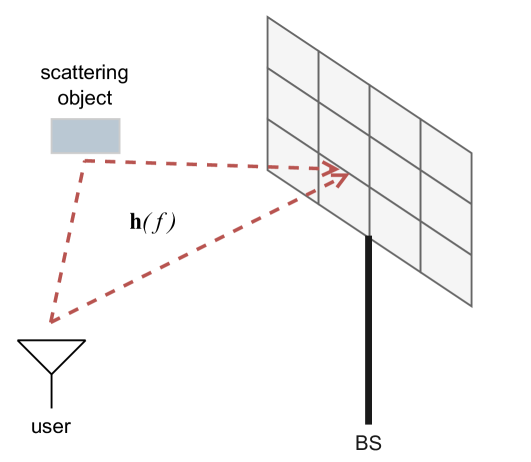
(a) Uplink setup

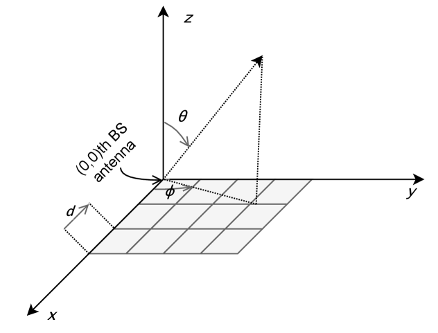
(b) Array geometry

Figure 1: Illustration of the BS antenna array and its geometry considered in the system model.

TABLE I: Main Notation Used in the System Model

Notation	Description
$N_{B}$	Number of BS antennas
$N_{\text{RF}}$	Number of RF chains
$S$	Number of subcarriers
$f_{s}$	Frequency of the $s$th subcarrier
$B$	Total signal bandwidth
$L$	Number of NLoS paths
$\alpha_{l}(f)$	Frequency-selective attenuation of the $l$th path
$\tau_{l}$	ToA of the $l$th path
$(\phi_{l},\theta_{l})$	DoA of the $l$th path
$\tau_{l,nm}$	Time delay to the $(n,m)$th BS antenna over the $l$th path
$\tau_{nm}(\phi_{l},\theta_{l})$	Time delay from the $(0,0)$th to the $(n,m)$th BS antenna
$\mathtt{x}(t)$	Baseband-equivalent of transmitted signal
$x(f)$	Fourier transform of $\mathtt{x}(t)$
$\mathtt{x}_{l}(t)$	Distorted version of $\mathtt{x}(t)$ over the $l$th path
$\tilde{r}_{nm}(t)$	Passband signal received by the $(n,m)$th BS antenna
$\mathtt{r}_{nm}(t)$	Baseband-equivalent of $\tilde{r}_{nm}(t)$
$r_{nm}(f)$	Fourier transform of $\mathtt{r}_{nm}(t)$
$d$	Antenna spacing
$f_{c}$	Carrier frequency
$c$	Speed of light
$k_{\text{abs}}$	Molecular absorption coefficient
$\mathtt{D}$	Distance between the BS and the user
$\Gamma_{l}(f)$	Reflection coefficient of the $l$th NLoS path

II System Model

Consider the uplink of a THz massive MIMO system where the BS is equipped with an $N\times M$-element UPA, and serves a single-antenna user as depicted in Fig 1(1(a)); the multi-antenna user case is investigated in Section V. The total number of BS antennas is $N_{B}=NM$, and the baseband frequency response of the uplink channel is denoted by $\mathbf{h}(f)\in\mathbb{C}^{N_{B}\times 1}$. In the sequel, we present the channel and hybrid transceiver models used in this work.

II-A THz Channel Model with Spatial-Wideband Effects

Due to limited scattering in THz bands, the propagation channel is represented by a ray-based model of $L+1$ rays [21], [23]. Hereafter, we assume that the $0$th ray corresponds to the LoS path, while the remaining $l=1,\dots,L$, rays are non-line-of-sight (NLoS) paths. Specifically, each path $l=0,\dots,L$, is characterized by its frequency-selective path attenuation $\alpha_{l}(f)$, time-of-arrival (ToA) $\tau_{l}$, and DoA $(\phi_{l},\theta_{l})$, where $\phi_{l}\in[-\pi,\pi]$ and $\theta_{l}\in[-\frac{\pi}{2},\frac{\pi}{2}]$ are the azimuth and polar angles, respectively. In the far-field region of the BS antenna array, the total delay between the user and the $(n,m)$th BS antenna through the $l$th path, $\tau_{l,nm}$, is calculated as

$${}\tau_{l,nm}=\tau_{l}+\tau_{nm}(\phi_{l},\theta_{l}),$$ (1)

where $\tau_{nm}(\phi_{l},\theta_{l})$ accounts for the propagation delay across the BS array, and is measured with respect to the $(0,0)$th BS antenna. For a UPA placed in the $xy$-plane (see Fig. 1(1(b))), we then have [24]

$$\tau_{nm}(\phi_{l},\theta_{l})\triangleq\frac{d(n\sin\theta_{l}\cos\phi_{l}+m\sin\theta_{l}\sin\phi_{l})}{c},$$ (2)

where $d$ is the antenna separation, and $c$ is the speed of light. The channel frequency response is derived as follows. Let $\mathtt{x}(t)$ be the baseband signal transmitted by the user, with $\mathcal{F}\{\mathtt{x}(t)\}=x(f)$. The passband signal, $\tilde{r}_{nm}(t)$, received by the $(n,m)$th BS antenna is written in the noiseless case as [25]

$$\tilde{r}_{nm}(t)=\sum_{l=0}^{L}\sqrt{2}\text{Re}\left\{\mathtt{x}_{l}(t-\tau_{l,nm})e^{j2\pi f_{c}(t-\tau_{l,nm})}\right\},$$ (3)

where $f_{c}$ is the carrier frequency, $\mathtt{x}_{l}(t)\triangleq\mathtt{x}(t)\ast\chi_{l}(t)$ is the distorted baseband waveform due to the frequency-selective attenuation of the $l$th path, and $\chi_{l}(t)$ models the said distortion; namely, $\mathcal{F}\{\chi_{l}(t)\}=\alpha_{l}(f)$ and $\mathcal{F}\{\mathtt{x}_{l}(t)\}=\alpha_{l}(f)x(f)$ [26]. Next, the received passband signal $\tilde{r}_{nm}(t)$ is down-converted to the baseband signal $\mathtt{r}_{nm}(t)$, which is given by

$$\mathtt{r}_{nm}(t)=\sum_{l=0}^{L}e^{-j2\pi f_{c}\tau_{l}}e^{-j2\pi f_{c}\tau_{nm}(\phi_{l},\theta_{l})}\mathtt{x}_{l}(t-\tau_{l,nm}).$$ (4)

Taking the continuous-time Fourier transform of (4) yields

$$r_{nm}(f) =\mathcal{F}\{\mathtt{r}_{nm}(t)\}$$

$$=\sum_{l=0}^{L}\beta_{l}(f)e^{-j2\pi(f_{c}+f)\tau_{nm}(\phi_{l},\theta_{l})}x(f)e^{-j2\pi f\tau_{l}},$$ (5)

where $\beta_{l}(f)\triangleq\alpha_{l}(f)e^{-j2\pi f_{c}\tau_{l}}$ is the complex gain of the $l$th path. Lastly, collecting all $r_{nm}(f)$ into a vector $\mathbf{r}(f)\in~{}\mathbb{C}^{N_{B}\times 1}$ gives the relation $\mathbf{r}(f)=\mathbf{h}(f)x(f)$, where

$$\mathbf{h}(f)=\sum_{l=0}^{L}\beta_{l}(f)\mathbf{a}(\phi_{l},\theta_{l},f)e^{-j2\pi f\tau_{l}}$$ (6)

is the baseband frequency response of the uplink channel, and

$$\mathbf{a}(\phi,\theta,f)=\left[1,\dots,e^{-j2\pi(f_{c}+f)\frac{d}{c}(n\sin\theta\cos\phi+m\sin\theta\sin\phi)}\right.,\\ \left.\dots,e^{-j2\pi(f_{c}+f)\frac{d}{c}((N-1)\sin\theta\cos\phi+(M-1)\sin\theta\sin\phi)}\right]^{T}$$ (7)

is the array response vector of the BS. Here, the array response is frequency-dependent due to the spatial-wideband effect.

We now introduce the path attenuation model. First, the so-called molecular absorption loss is no longer negligible at THz frequencies. Therefore, the path attenuation of the LoS path is calculated as [27]

$$|\beta_{0}(f)|=\alpha_{0}(f)=\frac{c}{4\pi(f_{c}+f)\mathtt{D}}e^{-\frac{1}{2}k_{\text{abs}}(f_{c}+f)\mathtt{D}},$$ (8)

where $\mathtt{D}$ denotes the distance between the BS and the user, and $k_{\text{abs}}(\cdot)$ is the molecular absorption coefficient determined by the composition of the propagation medium; different from mmWave channels, the major molecular absorption in THz bands comes from water vapor molecules [27]. For the NLoS paths, we consider single-bounce reflected rays, since the diffused and diffracted rays are heavily attenuated for distances larger than a few meters [28]. To this end, the reflection coefficient, $\Gamma_{l}(f)$, should be taken into account, which is specified as [29]

$$\Gamma_{l}(f)=\frac{\cos\phi_{i,l}-n_{t}\cos\phi_{t,l}}{\cos\phi_{i,l}+n_{t}\cos\phi_{t,l}}e^{-\left(\frac{8\pi^{2}(f_{c}+f)^{2}\sigma^{2}_{\text{rough}}\cos^{2}\phi_{i,l}}{c^{2}}\right)},$$ (9)

where $n_{t}\triangleq Z_{0}/Z$ is the refractive index, $Z_{0}=377$ Ohm is the free-space impedance, $Z$ is the impedance of the reflecting material, $\phi_{i,l}$ is the incidence and reflection angle, $\phi_{t,l}=\text{arcsin}\left(n^{-1}_{t}\sin\phi_{i,l}\right)$ is the refraction angle, and $\sigma_{\text{rough}}$ characterizes the roughness of the reflecting surface. The path attenuation of the $l$th NLoS path is finally given by [30]

$$|\beta_{l}(f)|=\alpha_{l}(f)=|\Gamma_{l}(f)|\alpha_{0}(f),$$ (10)

where $l=1,\dots,L$.

II-B Hybrid Transceiver Model

Due to the frequency selectivity of the THz channel, OFDM modulation is employed to combat inter-symbol interference. Specifically, we consider $S$ subcarriers over a signal bandwidth $B$. Then, the baseband frequency of the $s$th subcarrier is specified as $f_{s}=\left(s-\frac{S-1}{2}\right)\frac{B}{S},s=0,\dots,S-1$. A hybrid analog-digital architecture with $N_{\text{RF}}\ll N_{B}$ RF chains is also considered at the BS to facilitate efficient hardware implementation; each RF chain drives the array through $N_{B}$ analog phase shifters, as shown in Fig. 2. The hybrid combiner for the $s$th subcarrier is hence expressed as $\mathbf{F}[s]=\mathbf{F}_{\text{RF}}\mathbf{F}_{\text{BB}}[s]\in\mathbb{C}^{N_{B}\times N_{\text{RF}}}$, where $\mathbf{F}_{\text{RF}}\in\mathbb{C}^{N_{B}\times N_{\text{RF}}}$ is the frequency-flat RF combiner with elements of constant amplitude, i.e., $\frac{1}{\sqrt{N_{B}}}$, but variable phase, and $\mathbf{F}_{\text{BB}}[s]\in\mathbb{C}^{N_{\text{RF}}\times N_{\text{RF}}}$ is the baseband combiner. Finally, the post-processed baseband signal, $\mathbf{y}[s]\in\mathbb{C}^{N_{\text{RF}}\times 1}$, for the $s$th subcarrier is written as

$$\mathbf{y}[s] =\mathbf{F}^{H}[s]\mathbf{r}[s]$$

$$=\mathbf{F}^{H}[s]\left(\sqrt{P_{d}}\mathbf{h}[s]x[s]+\mathbf{n}[s]\right),$$ (11)

where $\mathbf{r}[s]\triangleq\mathbf{r}(f_{s})$ and $\mathbf{h}[s]\triangleq\mathbf{h}(f_{s})$ are the received signal and uplink channel, respectively, $x[s]\triangleq x(f_{s})\sim\mathcal{CN}(0,1)$ is the data symbol transmitted at the $s$th subcarrier, $P_{d}$ denotes the average power per data subcarrier assuming equal power allocation among subcarriers, and $\mathbf{n}[s]\sim\mathcal{CN}(\mathbf{0},\sigma^{2}\mathbf{I}_{N_{B}})$ is the additive noise vector.

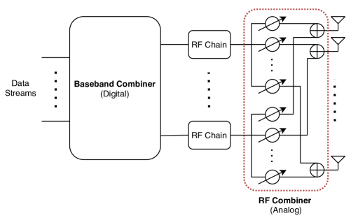
Figure 2: Illustration of the hybrid array structure considered in the system model.

Remark 1.

A promising alternative to OFDM is single-carrier with frequency domain equalization (SC-FDE) due to its favorable peak-to-average power ratio (PAPR). In our work, we exploit the inherent characteristics of THz channels, i.e., high path loss and directional transmissions, which result in a coherence bandwidth of hundreds of MHz [28]. Therefore, a relatively small number of subcarriers is used, which is expected to yield a tolerant PAPR.

III Hybrid Combining

III-A The Beam Squint Problem

Even for a moderate number of BS antennas, the propagation delay across the array can exceed the sampling period due to the ultra-high bandwidth used in THz communication. As a result, the DoA/DoD varies across the OFDM subcarriers, and the array gain becomes frequency-selective. This phenomenon, known as beam squint in the array processing literature, calls for a frequency-dependent combining design which is feasible only in a fully-digital array architecture.

To demonstrate the detrimental effect of beam squint when frequency-flat RF combining is employed, we consider an arbitrary ray impinging on the BS array with DoA $(\phi,\theta)$; therefore, we omit the subscript “$l$’ hereafter. In the narrowband case, the uplink channel is described as $\beta\mathbf{a}(\phi,\theta,0)$. Let $\mathbf{f}_{\text{RF}}=(1/\sqrt{N_{B}})\mathbf{f}$, with $\|\mathbf{f}\|^{2}=N_{B}$, be an arbitrary RF combiner. For the combiner $\mathbf{f}_{\text{RF}}$, the power of the received signal is calculated as

$$|\beta|^{2}\frac{\left|\mathbf{f}^{H}\mathbf{a}(\phi,\theta,0)\right|^{2}}{N_{B}}P_{d}=|\beta|^{2}N_{B}G(\phi,\theta,0)P_{d},$$ (12)

where $G(\phi,\theta,f)\triangleq|\mathbf{f}^{H}\mathbf{a}(\phi,\theta,f)|^{2}/N_{B}^{2}$ is the normalized array gain. Choosing $\mathbf{f}=\mathbf{a}(\phi,\theta,0)$ yields $G(\phi,\theta,0)=1$, and the maximum array gain is obtained. In a wideband THz system, though, the array gain varies across the OFDM subcarriers. In particular, we have that

$$G(\phi,\theta,f) =\frac{|\mathbf{a}^{H}(\phi,\theta,0)\mathbf{a}(\phi,\theta,f)|^{2}}{N_{B}^{2}}$$

$$=\left|D_{N}(2\pi f\Delta_{x}(\phi,\theta))\right|^{2}\left|D_{M}(2\pi f\Delta_{y}(\phi,\theta))\right|^{2},$$ (13)

where $\Delta_{x}(\phi,\theta)\triangleq(d\sin\theta\cos\phi)/c$ and $\Delta_{y}(\phi,\theta)\triangleq(d\sin\theta\sin\phi)/c$; please refer to Appendix A for the proof. Figure 3 shows the array gain for various bandwidths, when the narrowband RF combiner $\mathbf{f}_{\text{RF}}=1/(\sqrt{N_{B}})\mathbf{a}(\phi,\theta,0)$ is used. As we see, the array gain reduces substantially across the OFDM subcarriers. Furthermore, using the technique of [31], one can show that $G(\phi,\theta,f)\to 0$ as $NM\to\infty$. Contrary to narrowband massive MIMO, where the signal power increases monotonically with the number of BS antennas, here it may decrease. Consequently, beam squint compensation is of paramount importance for the successful deployment of THz massive MIMO systems.

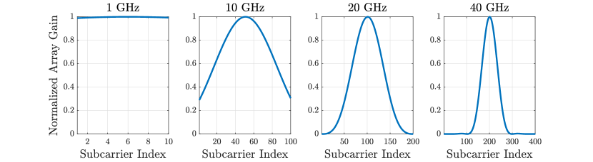
Figure 3: Normalized array gain for various bandwidths; $100\times 100$-element UPA, $f_{c}=300$ GHz, coherence bandwidth of $100$ MHz, and $(\phi,\theta)=(\pi/3,\pi/4)$.

III-B Proposed Combiner for Single-Path Channels

In this section, we introduce our wideband combining scheme for single-path channels, and then extend it to the multi-path case. To this end, we consider that the BS employs a single RF chain to combine the incoming signal, and hence the RF combiner is denoted by $\mathbf{f}_{\text{RF}}$. Next, we analyze the normalized array gain by decomposing the array into $N_{\text{sb}}\times M_{\text{sb}}$ virtual subarrays of $\tilde{N}\tilde{M}$ antennas each, where $\tilde{N}\triangleq N/N_{\text{sb}}$ and $\tilde{M}\triangleq M/M_{\text{sb}}$.

III-B1 Virtual Array Partition

The array response vector in (7) is decomposed as

$$\mathbf{a}(\phi,\theta,f)=\mathbf{a}_{x}(\phi,\theta,f)\otimes\mathbf{a}_{y}(\phi,\theta,f),$$ (14)

where $\mathbf{a}_{x}(\cdot)$ and $\mathbf{a}_{y}(\cdot)$ are defined, respectively, as

$$\mathbf{a}_{x}(\phi,\theta,f)\triangleq\left[1,\dots,e^{-j2\pi(f_{c}+f)n\Delta_{x}(\phi,\theta)},\right.\\ \left.\dots,e^{-j2\pi(f_{c}+f)(N-1)\Delta_{x}(\phi,\theta)}\right]^{T}$$ (15)

and

$$\mathbf{a}_{y}(\phi,\theta,f)\triangleq\left[1,\dots,e^{-j2\pi(f_{c}+f)m\Delta_{y}(\phi,\theta)},\right.\\ \left.\dots,e^{-j2\pi(f_{c}+f)(M-1)\Delta_{y}(\phi,\theta)}\right]^{T}.$$ (16)

Using the previously mentioned virtual array partition, we can write

$$\mathbf{a}_{x}(\phi,\theta,f) =\left[\mathbf{a}_{x,1}(\phi,\theta,f),\dots,\mathbf{a}_{x,N_{\text{sb}}}(\phi,\theta,f)\right]^{T},$$ (17)

$$\mathbf{a}_{y}(\phi,\theta,f) =\left[\mathbf{a}_{y,1}(\phi,\theta,f),\dots,\mathbf{a}_{y,M_{\text{sb}}}(\phi,\theta,f)\right]^{T},$$ (18)

where $\mathbf{a}_{x,n}(\phi,\theta,f)$ corresponds to the response vector of the $n$th virtual subarray, and is defined as

$$\mathbf{a}_{x,n}(\phi,\theta,f)\triangleq\left[e^{-j2\pi(f_{c}+f)(n-1)\tilde{N}\Delta_{x}(\phi,\theta)},\right.\\ \left.\dots,e^{-j2\pi(f_{c}+f)(n\tilde{N}-1)\Delta_{x}(\phi,\theta)}\right]^{T}.$$ (19)

Finally, each vector $\mathbf{a}_{x,n}(\phi,\theta,f)$ is expressed in terms of $\mathbf{a}_{x,1}(\phi,\theta,f)$, i.e., the response of the first subarray, as

$$\mathbf{a}_{x,n}(\phi,\theta,f)=e^{-j2\pi(f_{c}+f)(n-1)\tilde{N}\Delta_{x}(\phi,\theta)}\mathbf{a}_{x,1}(\phi,\theta,f).$$ (20)

$$G(\phi,\theta,f) =\frac{\left|\mathbf{a}^{H}_{x,1}(\phi,\theta,0)\mathbf{a}_{x,1}(\phi,\theta,f)\right|^{2}\left|\mathbf{a}^{H}_{y,1}(\phi,\theta,0)\mathbf{a}_{y,1}(\phi,\theta,f)\right|^{2}}{\tilde{N}^{2}\tilde{M}^{2}}\underbrace{\frac{\left|\sum_{n=1}^{N_{\text{sb}}}\sum_{m=1}^{M_{\text{sb}}}e^{-j2\pi(n-1)\tilde{N}f\Delta_{x}(\phi,\theta)}e^{-j2\pi(m-1)\tilde{M}f\Delta_{y}(\phi,\theta)}\right|^{2}}{N^{2}_{\text{sb}}M^{2}_{\text{sb}}}}_{\Omega(\phi,\theta,f)}$$

$$=\left|D_{\tilde{N}}(2\pi f\Delta_{x}(\phi,\theta))\right|^{2}\left|D_{\tilde{M}}(2\pi f\Delta_{y}(\phi,\theta))\right|^{2}\Omega(\phi,\theta,f).$$ (21)

We stress that similar expressions hold for the vector $\mathbf{a}_{y}$. Using the virtual subarray notation, the normalized array gain $G(\phi,\theta,f)$ is recast as in (III-B1) at the bottom of the next page. For an adequately small $\tilde{N}\tilde{M}$, we then have the approximation $D_{\tilde{N}}(2\pi f_{s}\Delta_{x}(\phi,\theta))D_{\tilde{M}}(2\pi f_{s}\Delta_{y}(\phi,\theta))\approx 1$.

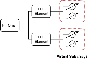
Figure 4: Illustration of the TTD-based wideband combiner with virtual array partition; the circles with arrows represent frequency-flat phase shifters.

III-B2 Size of Virtual Subarrays

The size of each virtual subarray, $\tilde{N}\times\tilde{M}$, is selected such that the maximum delay across the first virtual subarray is smaller than the sampling period $1/B$. Specifically, the maximum delay, $\tau_{\max}$, across the first subarray is given by (2) for $n=\tilde{N}-1$, $m=\tilde{M}-1$, $\sin\theta=1$, and $\sin\phi=\cos\phi=1/\sqrt{2}$, yielding $\tau_{\max}=d(\tilde{N}+\tilde{M}-2)/(\sqrt{2}c)$. For half-wavelength antenna spacing and $\tilde{N}=\tilde{M}$, the condition $\tau_{\max}<1/B$ reduces to $(\tilde{N}-1)<\sqrt{2}f_{c}/B$, which is used to determine $\tilde{N}$.

III-B3 TTD-Based Combining

The factor $\Omega(\phi,\theta,f)\leq 1$ in (III-B1) accounts for the losses caused by the delay between consecutive virtual subarrays, and it can be canceled through a TTD network placed between virtual subarrays, as depicted in Fig. 4. Then, we obtain $\Omega(\phi,\theta,f_{s})=1$ by multiplying the signal at the $(n,m)$th virtual subarray by $e^{j2\pi f_{s}\Delta_{mn}(\phi,\theta)}$, where $\Delta_{mn}(\phi,\theta)\triangleq(n-1)\tilde{N}\Delta_{x}(\phi,\theta)+(m-1)\tilde{M}\Delta_{y}(\phi,\theta)$ is the delay to be mitigated. Because all OFDM subcarriers share the same delay $\Delta_{mn}(\phi,\theta)$, it can be compensated using a single TTD element modeled as a linear filter with impulse response $\delta(t-\Delta_{nm}(\phi,\theta))$. Therefore, the wideband RF combiner is designed as

$$\mathbf{f}_{\text{RF}}[s]=\frac{1}{\sqrt{N_{B}}}\text{vec}\left(\mathbf{A}(\phi,\theta,0)\odot\mathbf{T}[s]\right),$$ (22)

where $\mathbf{T}[s]\triangleq\left[e^{-j2\pi f_{s}\Delta_{mn}(\phi,\theta)}\right]_{m=1,n=1}^{M_{\text{sb}},N_{\text{sb}}}\otimes\mathbf{1}_{\tilde{M}\times\tilde{N}}$, $\mathbf{A}(\phi,\theta,0)\triangleq\mathbf{a}_{y}(\phi,\theta,0)\mathbf{a}^{T}_{x}(\phi,\theta,0)$, and $\|\mathbf{f}_{\text{RF}}[s]\|^{2}=1$.

Proposition 1.

With the proposed combiner (22), we have

$$\left|\mathbf{f}^{H}_{\emph{RF}}\mathbf{a}(\phi,\theta,f)\right|^{2}=N_{B}\left|D_{\tilde{N}}(2\pi f\Delta_{x})\right|^{2}\left|D_{\tilde{M}}(2\pi f\Delta_{y})\right|^{2},$$ (23)

where $D_{N}(x)=\frac{\sin(Nx/2)}{N\sin(x/2)}$ is the Dirichlet sinc function.

Proof.

See Appendix B. ∎

From (23), we conclude that for sufficiently small $\tilde{N}$ and $\tilde{M}$, an array gain $N_{B}$ is approximately achieved over the whole signal bandwidth $B$. Thus, the SNR at the $s$th OFDM subcarrier is $|\beta(f_{s})|^{2}N_{B}P_{d}/\sigma^{2}$. Lastly, $(N_{\text{sb}}M_{\text{sb}}-1)$ TTD elements are employed per RF chain, where $N_{\text{sb}}=N/\tilde{N}$ and $M_{\text{sb}}=M/\tilde{M}$.

III-C Proposed Combiner for Multi-Path Channels

The propounded method can readily be applied to multi-path channels. For example, consider a THz channel comprising of $L=2$ NLoS paths. In a fully-digital array, the optimal combiner for the $s$th subcarrier is given by the maximum-ratio combiner $\mathbf{h}[s]/\|\mathbf{h}[s]\|$. By employing $N_{\text{RF}}=2$ RF chains, we have that

$$\frac{\mathbf{h}[s]}{\|\mathbf{h}[s]\|}=\mathbf{F}_{\text{RF}}[s]\mathbf{F}_{\text{BB}}[s]\mathbf{1}_{2\times 1},$$ (24)

where

$$\mathbf{F}_{\text{RF}}[s] =\frac{1}{\sqrt{N_{B}}}\begin{bmatrix}\mathbf{a}\left(\phi_{1},\theta_{1},f_{s}\right)&\mathbf{a}\left(\phi_{2},\theta_{2},f_{s}\right)\end{bmatrix},$$ (25)

$$\mathbf{F}_{\text{BB}}[s] =\frac{\sqrt{N_{B}}}{|\mathbf{h}[s]|}\begin{bmatrix}\beta_{1}(f_{s})e^{-j2\pi f_{s}\tau_{1}}&0\\ 0&\beta_{2}(f_{s})e^{-j2\pi f_{s}\tau_{2}}\end{bmatrix}.$$ (26)

The columns of the wideband RF combiner $\mathbf{F}_{\text{RF}}[s]$ are then approximated using (22), whilst the vector $\mathbf{1}_{2\times 1}$ with unit entries performs the addition of the two outputs of the baseband combiner. Note that $N_{\text{RF}}=L$ are required to implement the maximum-ratio combiner in a hybrid array architecture.

Remark 2.

A few recent papers in the literature (e.g., [32] and references therein) suggested the use of TTD to provide frequency-dependent phase shifts at each antenna of an $N\text{-element}$ ULA, yielding a wideband multi-beam architecture. In our work, we adopt a hybrid array architecture, where each frequency-independent phase shifter drives a single antenna whilst each TTD element controls a group of antennas, i.e., virtual subarray. Moreover, we consider a UPA, and hence our design enables squint-free three-dimensional (3D) combining.

IV Sparse Channel Estimation

We have introduced an effective wideband combiner assuming that the BS has perfect knowledge of the uplink channel. In this section, we investigate the channel estimation problem under the spatial-wideband effect. More particularly, we first formulate a compressive sensing problem to estimate the channel at each subcarrier independently with reduced training overhead. We then propound a wideband dictionary and employ an estimation algorithm that leverages information from multiple subcarriers to increase the reliability of the channel estimates in the low and moderate SNR regimes.

IV-A Problem Formulation

We assume a block-fading model where the channel coherence time is much larger than the training period. Specifically, the training period consists of $N_{\text{slot}}$ time slots. At each time slot $t=1,\dots,N_{\text{slot}}$, the user transmits the pilot signal $x_{t}[s]=\sqrt{P_{p}},\ \forall s\in\mathcal{S}$, where $\mathcal{S}\triangleq\{1,\dots,S\}$ denotes the set of OFDM subcarriers, and $P_{p}$ is the power per pilot subcarrier. In turn, the BS combines the pilot signal at each subcarrier $s\in\mathcal{S}$ using a training hybrid combiner $\mathbf{W}_{t}[s]\in\mathbb{C}^{N_{B}\times N_{\text{RF}}}$. Therefore, the post-processed signal at slot $t$, $\mathbf{y}_{t}[s]\in\mathbb{C}^{N_{\text{RF}}\times 1}$, is written as

$$\mathbf{y}_{t}[s]=\sqrt{P_{p}}\mathbf{W}_{t}^{H}[s]\mathbf{h}[s]+\mathbf{W}_{t}^{H}[s]\mathbf{n}_{t}[s],$$ (27)

where $\mathbf{n}_{t}[s]\sim\mathcal{CN}(\mathbf{0},\sigma^{2}\mathbf{I}_{N_{B}})$ is the additive noise vector. Let $N_{\text{beam}}=N_{\text{slot}}N_{\text{RF}}$ denote the total number of pilot beams. After $N_{\text{slot}}$ training slots, the BS acquires the measurement vector $\bar{\mathbf{y}}[s]\triangleq[\mathbf{y}^{T}_{1}[s],\dots,\mathbf{y}^{T}_{N_{\text{slot}}}[s]]^{T}\in\mathbb{C}^{N_{\text{beam}}\times 1}$ for $\mathbf{h}[s]$ as

$$\bar{\mathbf{y}}[s] =\sqrt{P_{p}}\begin{bmatrix}\mathbf{W}^{H}_{1}[s]\\ \vdots\\ \mathbf{W}^{H}_{N_{\text{slot}}}[s]\end{bmatrix}\mathbf{h}[s]+\begin{bmatrix}\mathbf{W}^{H}_{1}[s]\mathbf{n}_{1}[s]\\ \vdots\\ \mathbf{W}^{H}_{N_{\text{slot}}}[s]\mathbf{n}_{N_{\text{slot}}}[s]\end{bmatrix}$$

$$=\sqrt{P_{p}}\ \overline{\mathbf{W}}^{H}[s]\mathbf{h}[s]+\bar{\mathbf{n}}[s],$$ (28)

where $\overline{\mathbf{W}}[s]\triangleq[\mathbf{W}_{1}[s],\dots,\mathbf{W}_{N_{\text{slot}}}[s]]\in\mathbb{C}^{N_{B}\times N_{\text{beam}}}$, and $\bar{\mathbf{n}}[s]\in\mathbb{C}^{N_{\text{beam}}\times 1}$ denotes the effective noise. More particularly, $\mathbf{R}_{\bar{\mathbf{n}}[s]}\triangleq\sigma^{2}\text{diag}\left(\mathbf{W}^{H}_{1}[s]\mathbf{W}_{1}[s],\dots,\mathbf{W}^{H}_{N_{\text{slot}}}[s]\mathbf{W}_{N_{\text{slot}}}[s]\right)$ is the covariance matrix of the effective noise, which is colored in general. Regarding the pilot combiners, due to the hybrid array architecture, $\overline{\mathbf{W}}[s]=\overline{\mathbf{W}}_{\text{RF}}\overline{\mathbf{W}}_{\text{BB}}[s]$, with $\overline{\mathbf{W}}_{\text{RF}}=[\mathbf{W}_{\text{RF},1},\dots,\mathbf{W}_{\text{RF},N_{\text{slot}}}]\in\mathbb{C}^{N_{B}\times N_{\text{beam}}}$ containing the RF pilot beams and $\overline{\mathbf{W}}_{\text{BB}}[s]=\text{blkdiag}(\mathbf{W}_{\text{BB},1}[s],\dots,\mathbf{W}_{\text{BB},N_{\text{slot}}}[s])\in\mathbb{C}^{N_{\text{beam}}\times N_{\text{beam}}}$ comprising the $N_{\text{RF}}\times N_{\text{RF}}$ baseband combiners. The design of the pilot combiners is detailed in Section IV-D3.

IV-B Least Squares Estimator

From (IV-A), we have $N_{\text{beam}}$ observations, while $\mathbf{h}[s]$ includes $N_{B}$ variables. Thus, to obtain a good estimate of $\mathbf{h}[s]$, we need that $N_{\text{beam}}\geq N_{B}$. With this condition, the LS estimate is

$$\hat{\mathbf{h}}^{\text{LS}}[s]=\mathbf{Q}^{\dagger}_{s}\bar{\mathbf{y}}[s],$$ (29)

where $\mathbf{Q}_{s}\triangleq\sqrt{P_{p}}\ \overline{\mathbf{W}}^{H}[s]\in\mathbb{C}^{N_{\text{beam}}\times N_{B}}$ is the sensing matrix. The mean square error (MSE) of the LS estimator for the $s$th subcarrier is given by

$$J_{s}^{\text{LS}}\triangleq\mathbb{E}\left\{\left\|\mathbf{h}[s]-\hat{\mathbf{h}}^{\text{LS}}[s]\right\|^{2}\right\}=\text{tr}\left(\mathbf{Q}_{s}^{\dagger}\mathbf{R}_{\bar{\mathbf{n}}[s]}(\mathbf{Q}^{\dagger}_{s})^{H}\right).$$ (30)

The optimal $\mathbf{Q}_{s}$ satisfies $\mathbf{Q}^{H}_{s}\mathbf{Q}_{s}=P_{p}\mathbf{I}_{N_{B}}$ [34, 33]. In the hybrid array architecture under consideration, this is achieved by $\overline{\mathbf{W}}_{\text{BB}}[s]=\mathbf{I}_{N_{B}}$ and $\overline{\mathbf{W}}_{\text{RF}}=\mathbf{U}\in\mathbb{C}^{N_{B}\times N_{B}}$, where $\mathbf{U}$ is the DFT matrix generating the RF pilot beams [34]. We then have $\mathbf{R}_{\bar{\mathbf{n}}[s]}=\sigma^{2}\mathbf{I}_{N_{B}}$, $\mathbf{Q}_{s}^{\dagger}=(1/\sqrt{P_{p}})\mathbf{U}$, and

$$J_{s}^{\text{LS}}=\sigma^{2}N_{B}/P_{p}.$$ (31)

The LS estimator (29) requires $N_{\text{beam}}\geq N_{B}$, and hence yields a prohibitively high training overhead when the number of RF chains is much smaller than the number of BS antennas.

IV-C Sparse Formulation and Orthogonal Matching Pursuit

By exploiting the angular sparsity of THz channels, we can have a sparse formulation of the channel estimation problem as follows. The physical channel in (6) is also expressed as

$$\mathbf{h}[s]=\mathbf{A}[s]\bm{\beta}[s],$$ (32)

where $\mathbf{A}[s]\triangleq[\mathbf{a}(\phi_{0},\theta_{0},f_{s}),\dots,\mathbf{a}(\phi_{L},\theta_{L},f_{s})]\in~{}\mathbb{C}^{N_{B}\times(L+1)}$, with $\mathbf{a}(\phi_{l},\theta_{l},f_{s})$ being specified by (7) for $f=f_{s}$, is the so-called wideband array response matrix, and $\bm{\beta}[s]\triangleq[\beta_{0}(f_{s})e^{-j2\pi f_{s}\tau_{0}},\dots,\beta_{L}(f_{s})e^{-j2\pi f_{s}\tau_{L}}]^{T}\in\mathbb{C}^{(L+1)\times 1}$ is the vector of channel gains. Next, consider a dictionary $\bar{\mathbf{A}}[s]\in~{}\mathbb{C}^{N_{B}\times G}$ whose $G$ columns are the array response vectors associated with a predefined set of DoA. Then, the uplink channel can be approximated as

$$\mathbf{h}[s]\approx\bar{\mathbf{A}}[s]\bar{\bm{\beta}}[s],$$ (33)

where $\bar{\bm{\beta}}[s]\in\mathbb{C}^{G\times 1}$ has $L+1$ nonzero entries whose positions and values correspond to their DoA and path gains [35]. Therefore, (IV-A) is recast as

$$\bar{\mathbf{y}}[s]=\mathbf{\Phi}_{s}\bar{\bm{\beta}}[s]+\bar{\mathbf{n}}[s],$$ (34)

where $\mathbf{\Phi}_{s}\triangleq\sqrt{P_{p}}\ \overline{\mathbf{W}}^{H}[s]\bar{\mathbf{A}}[s]\in\mathbb{C}^{N_{\text{beam}}\times G}$ is the equivalent sensing matrix. Since $(L+1)\ll G$, the channel gain vector $\bar{\bm{\beta}}[s]$ is $(L+1)$-sparse, and the channel estimation problem can be formulated as the sparse recovery problem [34]

$$\hat{\bar{\bm{\beta}}}[s]=\arg \min_{\bar{\bm{\beta}}[s]}\ \|\bar{\bm{\beta}}[s]\|_{1}$$

$$\text{s.t.}\quad\left\|\bar{\mathbf{y}}[s]-\mathbf{\Phi}_{s}\bar{\bm{\beta}}[s]\right\|_{2}\leq\epsilon$$ (35)

where $\epsilon\leq\mathbb{E}\{\|\bar{\mathbf{n}}[s]\|_{2}\}$ is an appropriately chosen bound on the mean magnitude of the effective noise. The above optimization problem can be solved for each subcarrier independently, i.e., single measurement vector formulation. Finally, the estimate of $\mathbf{h}[s]$ is obtained as $\hat{\mathbf{h}}^{\text{CS}}[s]=\bar{\mathbf{A}}[s]\hat{\bar{\bm{\beta}}}[s]$.

Several greedy algorithms have been proposed to find approximate solutions of the $l_{1}$-norm optimization problem. The orthogonal matching pursuit (OMP) algorithm [36] described in Algorithm 1 is one of the most common and simple greedy CS methods that can solve (IV-C).

Algorithm 1 OMP-Based Estimator

1:Input: equivalent sensing matrix $\mathbf{\Phi}_{s}$ and measurement vector $\bar{\mathbf{y}}[s]$ for the $s$th subcarrier, and a threshold $\epsilon$.

2:$\mathcal{I}_{-1}=\emptyset$, $\mathcal{G}=\{1,\dots,G\}$, $\mathbf{r}_{-2}[s]=\mathbf{0}$, $\mathbf{r}_{-1}[s]=\bar{\mathbf{y}}[s]$, and $l=0$.

3:while $\|\mathbf{r}_{l-1}[s]-\mathbf{r}_{l-2}[s]\|^{2}>\epsilon$ do

4:     $g^{\star}=\underset{g\in\mathcal{G}}{\arg\max}\ \left|\mathbf{\Phi}_{s}^{H}(g)\mathbf{r}_{l-1}[s]\right|$

5:     $\mathcal{I}_{l}=\mathcal{I}_{l-1}\cup\{g^{\star}\}$

6:     $\mathbf{r}_{l}[s]=\left(\mathbf{I}_{N_{\text{beam}}}-\mathbf{\Phi}_{s}(\mathcal{I}_{l})\mathbf{\Phi}_{s}^{\dagger}(\mathcal{I}_{l})\right)\bar{\mathbf{y}}[s]$

7:     $l=l+1$

8:end while

9:$\hat{\bar{\bm{\beta}}}[s]=\mathbf{\Phi}_{s}^{\dagger}(\mathcal{I}_{l-1})\bar{\mathbf{y}}[s]$

10:return $\hat{\mathbf{h}}^{\text{CS}}[s]=\bar{\mathbf{A}}[s]\hat{\bar{\bm{\beta}}}[s]$.

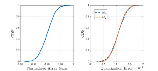
Figure 5: CDF of the normalized array gain and quantization error for a single-path channel and a super-resolution dictionary with $G_{x}=4N$ and $G_{y}=4M$; 1,000 channel realizations, $40\times 40$-element UPA, $\mathbf{f}_{\text{RF}}=(1/\sqrt{N_{B}})\mathbf{a}(\bar{\omega}_{x}(q),\bar{\omega}_{y}(p),f_{s})$, $B=40$ GHz, $S=400$ subcarriers, and $s=200$th subcarrier.

IV-D Proposed Channel Estimator

IV-D1 Wideband Dictionary for UPAs

For half-wavelength antenna separation, the array response vector (7) is recast as

$$\mathbf{a}(\omega_{x},\omega_{y},f)=\left[1,\dots,e^{-j2\pi\left(1+\frac{f}{f_{c}}\right)(n\omega_{x}+m\omega_{y})}\right.,\\ \dots,\left.e^{-j2\pi\left(1+\frac{f}{f_{c}}\right)\left((N-1)\omega_{x}+(M-1)\omega_{y}\right)}\right]^{T},$$ (36)

where $\omega_{x}=1/2\sin\theta\cos\phi$ and $\omega_{y}=1/2\sin\theta\sin\phi$ are the spatial frequencies [37]. The one-to-one mapping between the spatial frequencies $(\omega_{x},\omega_{y})$ and the physical angles $(\phi,\theta)$ is given by the relationships

$$\phi =\text{tan}^{-1}\left(\omega_{y}/\omega_{x}\right),$$ (37)

$$\theta =\text{sin}^{-1}\left(2\sqrt{\omega_{x}^{2}+\omega_{y}^{2}}\right).$$ (38)

Since both $\omega_{x}$ and $\omega_{y}$ lie in $[-1/2,1/2]$, we can consider the grids of discrete spatial frequencies

$$\mathcal{G}_{x} =\left\{\bar{\omega}_{x}(q)=q/G_{x},\ q=-(G_{x}-1)/2,\dots,(G_{x}-1)/2\right\},$$ (39)

$$\mathcal{G}_{y} =\{\bar{\omega}_{y}(p)=p/G_{y},\ p=-(G_{y}-1)/2,\dots,(G_{y}-1)/2\},$$ (40)

where $G_{x}G_{y}=G$ is the overall dictionary size.

For the $s$th subcarrier, we define the array response matrices $\bar{\mathbf{A}}_{x}[s]\in\mathbb{C}^{N\times G_{x}}$ and $\bar{\mathbf{A}}_{y}[s]\in\mathbb{C}^{M\times G_{y}}$ whose columns are the array response vectors $\mathbf{a}_{x}(\cdot,f_{s})$ and $\mathbf{a}_{y}(\cdot,f_{s})$ evaluated at the grid points of $\mathcal{G}_{x}$ and $\mathcal{G}_{y}$, respectively. Now, the dictionary $\bar{\mathbf{A}}[s]\triangleq\bar{\mathbf{A}}_{x}[s]\otimes\bar{\mathbf{A}}_{y}[s]\in\mathbb{C}^{N_{B}\times G}$ can be used to approximate the uplink channel $\mathbf{h}[s]$ at the $s$th subcarrier. Although this approximation entails quantization errors, they become small for large $G_{x}$ and $G_{y}$ [35]. More specifically, we can use a super-resolution dictionary with $G_{x}>N$ and $G_{y}>M$ to reduce the mismatch between the quantized and the actual channel. We evaluate the accuracy of the proposed dictionary by generating a DoA with $(\omega_{x},\omega_{y})$, which is then quantized to the closest value $(\bar{\omega}_{x}(q),\bar{\omega}_{y}(p))$. Figure 5 shows the cumulative distribution function (CDF) of the normalized array gain $\left|\mathbf{a}^{H}(\bar{\omega}_{x}(q),\bar{\omega}_{y}(p),f_{s})\mathbf{a}(\omega_{x},\omega_{y},f_{s})\right|^{2}/N_{B}^{2}$, and the quantization errors $|\omega_{x}-\bar{\omega}_{x}(q)|$ and $|\omega_{y}-\bar{\omega}_{y}(p)|$ of the spatial frequencies. As we observe, the errors are small, and do not affect significantly the normalized array gain. Consequently, we can neglect the quantization errors, and assume that the DoA of each path lies on the dictionary grid. Note that for $G_{x}=N$ and $G_{y}=M$, the dictionary $\bar{\mathbf{A}}[s]$ reduces to the known virtual channel representation (VCR) [38] in the spatial-narrowband case. Lastly, a similar representation, termed extended VCR, was introduced in [39] for narrowband massive MIMO systems.

IV-D2 Generalized Multiple Measurement Vector Problem

Due to the frequency-dependent dictionary, the channel gain vectors $\{\bar{\bm{\beta}}[s]\}_{s=0}^{S-1}$ share the same support. Therefore, we can exploit the common support property and consider the problem in (IV-C) as a generalized multiple measurement vector (GMMV) problem, where multiple sensing matrices are employed [40]. To tackle the GMMV problem, we employ the simultaneous OMP algorithm [41]. The proposed channel estimator is described in Algorithm 2.

Algorithm 2 GSOMP-Based Estimator

1:Input: set $\mathcal{S}$ of pilot subcarriers, sensing matrices $\mathbf{\Phi}_{s}$ and measurement vectors $\bar{\mathbf{y}}[s],\forall s\in\mathcal{S}$, and a threshold $\epsilon$.

2:$\mathcal{I}_{-1}=\emptyset$, $\mathcal{G}=\{1,\dots,G\}$, $\mathbf{r}_{-1}[s]=\bar{\mathbf{y}}[s]$, $\mathsf{MSE}=\sum_{s\in\mathcal{S}}\|\bar{\mathbf{y}}[s]\|^{2}$, and $l=0$.

3:while $\mathsf{MSE}>\epsilon$ do

4:     $g^{\star}=\underset{g\in\mathcal{G}\setminus\mathcal{I}_{l-1}}{\arg\max}\ \underset{s\in\mathcal{S}}{\sum}\left|\mathbf{\Phi}_{s}^{H}(g)\mathbf{r}_{l-1}[s]\right|$

5:     $\mathcal{I}_{l}=\mathcal{I}_{l-1}\cup\{g^{\star}\}$

6:     $\mathbf{r}_{l}[s]=\left(\mathbf{I}_{N_{\text{beam}}}-\mathbf{\Phi}_{s}(\mathcal{I}_{l})\mathbf{\Phi}_{s}^{\dagger}(\mathcal{I}_{l})\right)\bar{\mathbf{y}}[s],\ \forall s\in\mathcal{S}$

7:     $\mathsf{MSE}=\frac{1}{|\mathcal{S}|}\sum_{s\in\mathcal{S}}\|\mathbf{r}_{l}[s]-\mathbf{r}_{l-1}[s]\|^{2}$

8:     $l=l+1$

9:end while

10:$\hat{\bar{\bm{\beta}}}[s]=\mathbf{\Phi}_{s}^{\dagger}(\mathcal{I}_{l-1})\bar{\mathbf{y}}[s],\forall s\in\mathcal{S}$

11:return $\hat{\mathbf{h}}^{\text{CS}}[s]=\bar{\mathbf{A}}[s]\hat{\bar{\bm{\beta}}}[s],\forall s\in\mathcal{S}$.

Regarding the stopping criterion of the OMP/GSOMP algorithm, we design the pilot combiners so that the effective noise is white. In this case, the variance of the noise power is $\mathbb{E}\left\{\|\bar{\mathbf{n}}[s]\|^{2}\right\}=N_{\text{beam}}\sigma^{2}$, and the threshold can be chosen as $\epsilon=N_{\text{beam}}\sigma^{2}$, or a fraction of the average noise power. Additionally, a thresholding step can be incorporated into the algorithms, in which only the entries of the estimate $\hat{\bar{\bm{\beta}}}$ with power higher than the noise variance will be selected as detected paths. After estimating the spatial frequencies of each path, the physical angles are obtained through (37) and (38), which are then used in the TTD-based wideband combiner.

IV-D3 Pilot Beam Design

The elements of the RF combiner $\overline{\mathbf{W}}_{\text{RF}}$ are selected from the set $\{-1/\sqrt{N_{B}},1/\sqrt{N_{B}}\}$ with equal probability. The reason we adopt a randomly formed RF combiner is that it has been shown to have a low mutual-column coherence, and therefore can be expected to attain a high recovery probability according to the compressive sensing theory [42]. The specific RF pilot design leads to a colored effective noise, however the SOMP algorithm is based on the assumption that the noise covariance matrix is diagonal. To this end, we design the baseband combiner such that the combined noise remains white. In particular, let $\mathbf{D}^{H}_{t}\mathbf{D}_{t}$ be the Cholesky decomposition of $\mathbf{W}^{H}_{\text{RF,t}}\mathbf{W}_{\text{RF,t}}$, where $\mathbf{D}\in\mathbb{C}^{N_{\text{RF}}\times N_{\text{RF}}}$ is an upper triangular matrix. Then, the baseband combiner of the $t$th slot is set to $\mathbf{W}_{\text{BB},t}[s]=\mathbf{D}^{-1}_{t}$, and hence $\overline{\mathbf{W}}[s]=\overline{\mathbf{W}}_{\text{RF}}\text{blkdiag}(\mathbf{D}^{-1}_{1},\dots,\mathbf{D}^{-1}_{N_{\text{slot}}})$. Under this pilot beam design, the covariance matrix of the effective noise becomes $\mathbf{R}_{\bar{\mathbf{n}}}=\sigma^{2}\mathbf{I}_{N_{\text{beam}}}$, yielding the desired result. We finally point out that the combiners $\overline{\mathbf{W}}[s]$ can be computed offline.

IV-E Performance of the Proposed Channel Estimator

IV-E1 Lower Bound Error Analysis

As previously mentioned, for semi-unitary combiners $\mathbf{W}_{t}[s]$ with $\mathbf{W}_{t}^{H}[s]\mathbf{W}_{t}[s]=\mathbf{I}_{N_{\text{RF}}},\forall t=1,\dots,N_{\text{slot}}$, the covariance matrix of the effective noise $\bar{\mathbf{n}}[s]$ is equal to $\sigma^{2}\mathbf{I}_{N_{\text{beam}}}$. Next, we derive the CRLB assuming that the GSOMP recovers the exact support of $\bar{\bm{\beta}}[s]$, i.e., $\mathcal{I}_{l-1}=\text{supp}\left(\bar{\bm{\beta}}[s]\right)$ = $\mathcal{I}$. To this end, we can define the following linear model for the $s$th subcarrier

$$\bar{\mathbf{y}}[s]=\mathbf{\Phi}_{s}(\mathcal{I})\tilde{\bar{\bm{\beta}}}[s]+\bar{\mathbf{n}}[s],$$ (41)

where $\tilde{\bar{\bm{\beta}}}[s]\in\mathbb{C}^{L\times 1}$ denotes the vector to be estimated, and $\bar{\mathbf{y}}[s]$ is distributed as $\mathcal{CN}\left(\mathbf{\Phi}_{s}(\mathcal{I})\tilde{\bar{\bm{\beta}}}[s],\sigma^{2}\mathbf{I}_{N_{\text{beam}}}\right)$. The model in (41) is linear on the parameter vector $\tilde{\bar{\bm{\beta}}}[s]$, and the solution $\hat{\bar{\bm{\beta}}}[s]=\mathbf{\Phi}_{s}^{\dagger}(\mathcal{I})\bar{\mathbf{y}}[s]$ gives $\mathbb{E}\left\{\hat{\bar{\bm{\beta}}}[s]\right\}=\tilde{\bar{\bm{\beta}}}[s]$. Specifically, $\hat{\bar{\bm{\beta}}}[s]$ is the mininum variance unbiased estimator of $\tilde{\bar{\bm{\beta}}}[s]$, hence attaining the CRLB [43]. Next, the Fisher information matrix for (41) is calculated as

$$\mathbf{I}\left(\tilde{\bar{\bm{\beta}}}[s]\right)=\frac{1}{\sigma^{2}}\mathbf{\Phi}^{H}_{s}(\mathcal{I})\mathbf{\Phi}_{s}(\mathcal{I}).$$ (42)

The channel estimate for the $s$th subcarrier is acquired as $\hat{\mathbf{h}}^{\text{CS}}[s]=\bar{\mathbf{A}}_{s}(\mathcal{I})\hat{\bar{\bm{\beta}}}[s]$, where $\bar{\mathbf{A}}_{s}(\mathcal{I})$ denotes the matrix with the columns of $\bar{\mathbf{A}}[s]$ given by the support $\mathcal{I}$. Let $J^{\text{CS}}_{s}$ denote the MSE of the OMP. Since $\mathbb{E}\left\{\hat{\mathbf{h}}^{\text{CS}}\right\}=\bar{\mathbf{A}}_{s}(\mathcal{I})\tilde{\bar{\bm{\beta}}}[s]\triangleq\bm{\psi}\left(\tilde{\bar{\bm{\beta}}}[s]\right)$, the CRLB for the $s$th subcarrier is given by [43]

$$J^{\text{CS}}_{s}\geq\text{tr}\left\{\ \frac{\partial\bm{\psi}\left(\tilde{\bar{\bm{\beta}}}[s]\right)}{\partial\tilde{\bar{\bm{\beta}}}[s]}\mathbf{I}^{-1}\left(\tilde{\bar{\bm{\beta}}}[s]\right)\frac{\partial\bm{\psi}^{H}\left(\tilde{\bar{\bm{\beta}}}[s]\right)}{\partial\tilde{\bar{\bm{\beta}}}[s]}\right\},$$ (43)

where $\partial\bm{\psi}\left(\tilde{\bar{\bm{\beta}}}[s]\right)/\partial\tilde{\bar{\bm{\beta}}}[s]=\bar{\mathbf{A}}_{s}(\mathcal{I})$.

IV-E2 Complexity Analysis

In this section, we detail the computational complexity per iteration $l$ of the GSOMP scheme. Specifically, we have the following operations:

• The $l_{2}$-norm operations at step $1$ and step $6$ have $\mathcal{O}(|\mathcal{S}|N_{\text{beam}})$ complexity.

• The calculation of the product $\mathbf{\Phi}_{s}^{H}(g)\mathbf{r}_{l-1}[s]$ at step $3$ is $\mathcal{O}(|\mathcal{S}|N_{\text{beam}}(G-l))$ because there are $G-l$ elements to examine at the $l$th iteration, where $G$ is the size of the dictionary.

• To find the maximum element from $G-l$ values at step $3$ is on the order of $\mathcal{O}(G-l)$.

• The LS operation at step $5$ is $\mathcal{O}(l^{3}+2l^{2}N_{\text{beam}})$ for each pilot subcarrier. This is because $\mathbf{\Phi}(\mathcal{I}_{l})$ is a $N_{\text{beam}}\times l$ matrix, and hence its pseudoinverse entails $l^{3}+l^{2}N_{\text{beam}}$ operations plus the multiplication with $\mathbf{\Phi}(\mathcal{I}_{l})$ entailing $l^{2}N_{\text{beam}}$ additional multiplications.

Given the above, the overall online computational complexity is $\mathcal{O}\left(|\mathcal{S}|(N_{\text{beam}}(G-l)+l^{3}+2l^{2}N_{\text{beam}})+(G-l)\right)$. Note that the OMP has $\mathcal{O}(|\mathcal{S}|G)$ at step $3$ for finding the maximum correlation between the measurement vector and the columns of the dictionary. As a result, the GSOMP leads to a computational reduction as well.

V The Multi-Antenna User Case

We now discuss how the previous analysis can be extended to the case of a multi-antenna user. To this end, we consider a user with an $N_{U}$-element ULA. The frequency response of the uplink channel, $\mathbf{H}(f)\in\mathbb{C}^{N_{B}\times N_{U}}$, is then expressed as

$$\mathbf{H}(f)=\sum_{l=0}^{L}\beta_{l}(f)\mathbf{a}_{B}(\phi_{l},\theta_{l},f)\mathbf{a}^{H}_{U}(\varphi_{l},f)e^{-j2\pi f\tau_{l}},$$ (44)

where $\mathbf{a}_{B}(\cdot,\cdot,\cdot)$ denotes the response vector (7) of the BS array, $\varphi_{l}$ is the angle-of-departure (AoD) of the $l$th path from the user, and

$$\mathbf{a}_{U}(\varphi,f)\triangleq\left[1,e^{-j2\pi\left(f_{c}+f\right)\frac{d}{c}\sin\varphi},\right.\\ \left.\dots,e^{-j2\pi(f_{c}+f)(N_{U}-1)\frac{d}{c}\sin\varphi}\right]^{T}$$ (45)

is the wideband response vector of the user array.

At the BS, the post-processed baseband signal for the $s$th subcarrier is expressed as

$$\mathbf{y}[s]=\mathbf{F}^{H}[s]\left(\mathbf{H}[s]\mathbf{B}[s]\tilde{\mathbf{x}}[s]+\mathbf{n}[s]\right),$$ (46)

where $\mathbf{B}[s]\in\mathbb{C}^{N_{U}\times N^{u}_{\text{RF}}}$ is the hybrid precoder when the user employs $N^{u}_{\text{RF}}$ RF chains, $\tilde{\mathbf{x}}[s]=\mathbf{P}[s]\mathbf{x}[s]$ is the transmitted signal at the $s$th subcarrier, $\mathbf{P}[s]=\text{diag}(p_{1,s},\dots,p_{N^{u}_{\text{RF}},s})$ is the power allocation matrix, and $\mathbf{x}[s]\sim\mathcal{CN}(\mathbf{0},\mathbf{I}_{N^{u}_{\text{RF}}})$ is the vector of data symbols. Furthermore, the power constraint $\sum_{s=0}^{S-1}\mathbb{E}\left\{\|\mathbf{B}[s]\tilde{\mathbf{x}}[s]\|^{2}\right\}\leq P_{t}$ should be satisfied, so that the transmit power does not exceed the user’s power budget $P_{t}$.

V-A Hybrid Combining and Beamforming

Consider a single-path channel with AoD $\varphi$ from the user and DoA $(\phi,\theta)$ at the BS. For the frequency-flat beamformer $(1/\sqrt{N_{U}})\mathbf{a}_{U}(\varphi,0)$ and combiner $(1/\sqrt{N_{B}})\mathbf{a}_{B}(\phi,\theta,0)$, the normalized array gain in (III-A) is recast as in (V-A) at the bottom of this page, where $\Delta(\varphi)\triangleq d\sin\varphi/c$. Employing TTD-based combining and beamforming yields $G(\phi,\theta,\varphi,f)\approx~{}1$, and the SNR at the $s$th subcarrier is approximately equal to $|\beta(f_{s})|^{2}N_{U}N_{B}P_{d}/\sigma^{2}$. Compared to the single-antenna user case, we have an additional beamforming gain $N_{U}$.

$$G(\phi,\theta,\varphi,f) =\frac{|\mathbf{a}_{B}^{H}(\phi,\theta,0)\mathbf{a}_{B}(\phi,\theta,f)|^{2}}{N_{B}^{2}}\frac{|\mathbf{a}_{U}^{H}(\varphi,f)\mathbf{a}_{U}(\varphi,0)|^{2}}{N_{U}^{2}}$$

$$=\left|D_{N}(2\pi f\Delta_{x}(\phi,\theta))\right|^{2}\left|D_{M}(2\pi f\Delta_{y}(\phi,\theta))\right|^{2}\left|D_{N_{U}}(2\pi f\Delta(\varphi))\right|^{2}.$$ (47)

Now consider, for instance, a multi-path channel of $L=2$ NLoS paths. In a fully-digital array, the combiner and precoder maximizing the achievable rate are given by the singular value decomposition (SVD) of the channel matrix $\mathbf{H}[s]$ [11]. For our hybrid analog-digital array structure, we adopt a practical approach, as in [17]. We first decompose the channel matrix as $\mathbf{H}(f)=\mathbf{H}_{B}(f)\mathbf{H}^{H}_{U}(f)$, where

$$\mathbf{H}_{B}(f)=\begin{bmatrix}\mathbf{a}_{B}(\phi_{1},\theta_{1},f),&\mathbf{a}_{B}(\phi_{2},\theta_{2},f)\end{bmatrix},$$ (48)

and

$$\mathbf{H}_{U}(f)=\left[\beta_{1}(f)\mathbf{a}_{U}(\varphi_{1},f)e^{-j2\pi f\tau_{1}},\right.\\ \left.\beta_{2}(f)\mathbf{a}_{U}(\varphi_{2},f)e^{-j2\pi f\tau_{2}}\right].$$ (49)

Next, the RF combiner and beamformer are the matched filters of the channels $\mathbf{H}_{B}(f)$ and $\mathbf{H}^{H}_{U}(f)$, respectively, whereas the baseband combiner and precoder are designed using the SVD of the effective channel, when both ends have full CSI. Note that for a multi-path channel with $L>N_{\text{RF}}$ paths, the user communicates at most $\min(L,N_{\text{RF}})$ spatial streams to the BS in the absence of inter-stream interference through SVD-based transmission.

V-B Sparse Channel Estimation

The user employs a training codebook $\{\mathbf{v}_{i}\in\mathbb{C}^{N_{U}\times 1},i=1,\dots,N^{u}_{\text{beam}}\}$, which consists of $N_{\text{beam}}^{u}$ pilot RF beamformers. When the $i$th pilot beamformer is used during $N_{\text{slot}}$ training slots, (IV-A) is recast as

$$\bar{\mathbf{y}}_{i}[s]=\sqrt{P_{p}}\ \overline{\mathbf{W}}^{H}[s]\mathbf{H}[s]\mathbf{v}_{i}+\bar{\mathbf{n}}_{i}[s].$$ (50)

By collecting all vectors $\bar{\mathbf{y}}_{i}[s]$ into a single matrix $\mathbf{Y}[s]=[\bar{\mathbf{y}}_{1}[s],\dots,\bar{\mathbf{y}}_{N^{u}_{\text{beam}}}[s]]\in\mathbb{C}^{N_{\text{beam}}\times N^{u}_{\text{beam}}}$, we can write

$$\mathbf{Y}[s]=\sqrt{P_{p}}\ \overline{\mathbf{W}}^{H}[s]\mathbf{H}[s]\mathbf{V}+\mathbf{N}[s],$$ (51)

where $\mathbf{V}=[\mathbf{v}_{1},\dots,\mathbf{v}_{N^{u}_{\text{beam}}}]\in\mathbb{C}^{N_{U}\times N^{u}_{\text{beam}}}$, and $\mathbf{N}=[\bar{\mathbf{n}}_{1}[s],\dots,\bar{\mathbf{n}}_{N^{u}_{\text{beam}}}[s]]\in\mathbb{C}^{N_{\text{beam}}\times N^{u}_{\text{beam}}}$. Utilizing the identity $\text{vec}(\mathbf{A}\mathbf{B}\mathbf{C})=(\mathbf{C}^{T}\otimes\mathbf{A})\text{vec}(\mathbf{B})$, we express (51) in vector form as

$$\text{vec}(\mathbf{Y}[s])=\sqrt{P_{p}}\left(\mathbf{V}^{T}\otimes\overline{\mathbf{W}}^{H}[s]\right)\text{vec}(\mathbf{H}[s])+\text{vec}(\mathbf{N}[s]),$$ (52)

where $\text{vec}(\mathbf{Y}[s])\in\mathbb{C}^{N_{\text{beam}}N^{u}_{\text{beam}}\times 1}$ is the overall measurement vector, $\text{vec}(\mathbf{H}[s])\in\mathbb{C}^{N_{B}N_{U}\times 1}$ is the uplink channel to be estimated, and $\text{vec}(\mathbf{N}[s])\in\mathbb{C}^{N_{\text{beam}}N^{u}_{\text{beam}}\times 1}$ is the noise vector. Now, the proposed GSOMP-based estimator can readily be used by considering the equivalent sensing matrix $\mathbf{\Phi}_{s}=\sqrt{P_{p}}\left(\mathbf{V}^{T}\otimes\overline{\mathbf{W}}^{H}[s]\right)\bar{\mathbf{A}}[s]\in\mathbb{C}^{N_{\text{beam}}N^{u}_{\text{beam}}\times GG^{u}}$, where $\bar{\mathbf{A}}[s]\triangleq\bar{\mathbf{A}}^{*}_{u}[s]\otimes(\bar{\mathbf{A}}_{x}[s]\otimes\bar{\mathbf{A}}_{y}[s])\in\mathbb{C}^{N_{B}N_{U}\times GG^{u}}$ is the equivalent dictionary accounting also for the dictionary $\bar{\mathbf{A}}_{u}[s]\in\mathbb{C}^{N_{U}\times G^{u}}$ of size $G^{u}$ at the user side. Finally, the estimated channel is constructed as $\text{vec}(\hat{\mathbf{H}}[s])=\bar{\mathbf{A}}[s]\hat{\bar{\bm{\beta}}}[s]$.

TABLE II: Main Simulation Parameters [27, 28]

Parameter	Value
Bandwidth	$B=40$ GHz
Carrier frequency	$f_{c}=300$ GHz
Transmit power	$P_{t}=10$ dBm
Power density of noise	$\sigma^{2}=-174$ dBm/Hz
Azimuth AoA	$\phi_{l}\sim\mathcal{U}\left(-\pi,\pi\right)$
Polar AoA	$\theta_{l}\sim\mathcal{U}\left(-\pi/2,\pi/2\right)$
LoS path length	$\mathtt{D}=15$ m
ToA of LoS	$\tau_{0}=50$ nsec
ToA of NLoS	$\tau_{l}\sim\mathcal{U}(50,55)$ nsec
Absorption coefficient	$k_{\text{abs}}=0.0033\ \text{m}^{-1}$
Refractive index	$n_{t}=2.24-j0.025$
Roughness factor	$\sigma_{\text{rough}}=0.088\cdot 10^{-3}$ m

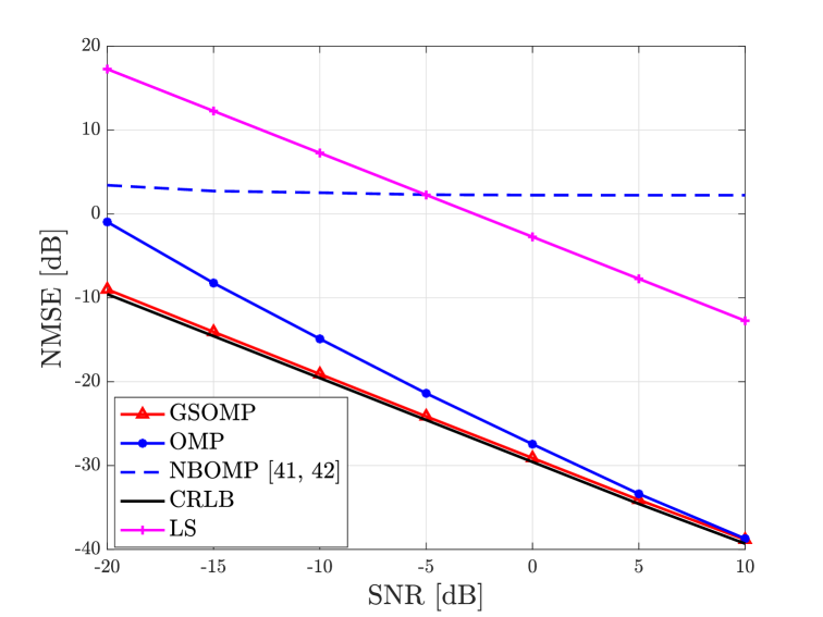
(a)

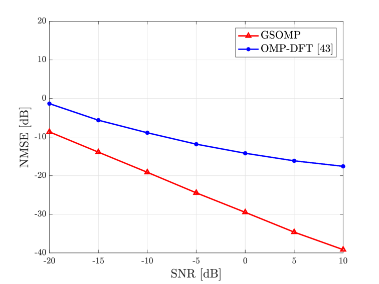
(b)

Figure 6: NMSE versus SNR for a single-antenna user. The OMP, NBOMP, and GSOMP estimators are evaluated under partial training of $N_{\text{beam}}=0.8N_{B}$ pilot beams; $40\times 40$-element UPA, $N_{\text{RF}}=2$, NLoS channel with $L=3$ paths, $S=400$ subcarriers, and super-resolution dictionary with $G=4N_{B}$.

VI Numerical Results

In this section, we conduct numerical simulations to evaluate the performance of the proposed channel estimator and hybrid combiner. To this end, we consider the following setup:

• Number of OFDM Subcarriers: For a NLoS multi-path scenario where $\tau_{l}\sim~{}\mathcal{U}(50,55)$ nsec, the delay spread is $D_{s}=5$ nsec. The coherence bandwidth is then calculated as $B_{c}=1/(2D_{s})=100$ MHz [25], which results in $S\approx B/B_{c}=400$ subcarriers. On the other hand, for a LoS scenario, the delay spread is equal to the maximum delay across the UPA due to the spatial-wideband effect. This results in $S\approx~{}18$ subcarriers for an $100\times 100$-element UPA and $B=40$ GHz.

• Antenna Gain: Each BS antenna element has a directional power pattern, $\Lambda(\phi,\theta)$, which is specified according to the 3GPP standard as [48]

  $$\Lambda(\phi,\theta)=\Lambda_{\max}-\min\left[-\Lambda_{H}(\phi)-\Lambda_{V}(\theta),\Lambda_{\text{FBR}}\right],$$ (53)

  where

  $$\Lambda_{H}(\phi) =-\min\left[12\left(\frac{\phi}{\phi_{\text{3dB}}}\right)^{2},\Lambda_{\text{FBR}}\right],$$ (54)

  $$\Lambda_{V}(\theta) =-\min\left[12\left(\frac{\theta-90\degree}{\theta_{\text{3dB}}}\right)^{2},\text{SLA}_{v}\right],$$ (55)

  where $\min\left[\cdot,\cdot\right]$ denotes the minimum between the input arguments, $\Lambda_{\max}$ is the maximum gain in the boresight direction, $\phi_{\text{3dB}}=65\degree$ and $\theta_{\text{3dB}}=65\degree$ are the horizontal and vertical half-power beamwidths, respectively, $\Lambda_{\text{FBR}}=30$ dB is the front-to-back ratio, and $\text{SLA}_{v}=30$ dB is the side lobe attenuation in the vertical direction. We choose $\Lambda_{\max}=50$ dBi [27]. At the user side, we assume omnidirectional antennas. The channel model is then recast by replacing $\mathbf{a}(\phi,\theta,f)$ with $\sqrt{\Lambda(\phi,\theta)}\mathbf{a}(\phi,\theta,f)$ [49].

The other simulation parameters are summarized in Table II.

VI-A Channel Estimation

VI-A1 Single-Antenna User

Our main performance metric is the normalized mean-square error (NMSE) versus the average receive SNR for the estimators intoduced previously. Specifically, for a given channel realization, the NMSE metric is defined as

$$\text{NMSE}\triangleq\frac{1}{|\mathcal{S}|}\sum_{s\in\mathcal{S}}\mathbb{E}\left\{\left\|\mathbf{h}[s]-\hat{\mathbf{h}}[s]\right\|^{2}\big{/}\|\mathbf{h}[s]\|^{2}\right\},$$ (56)

where $\hat{\mathbf{h}}[s]$ denotes the estimate of the corresponding estimator. The NMSE is computed numerically over 100 channel realizations. The channel gains $\{\beta_{l}(f_{s})\}_{l=1}^{L}$ are generated as $\mathcal{CN}(0,\sigma^{2}_{\beta})$, with $\sigma^{2}_{\beta}=10^{-9}$, i.e., $-90$ dB, modeling the high path attenuation at THz frequencies [23]. The average SNR is then calculated as $\text{SNR}=\sigma^{2}_{\beta}P_{p}/P_{n}$, where $P_{p}=P_{t}/|\mathcal{S}|$ is the power per pilot subcarrier, and $P_{n}=\Delta B\sigma^{2}$ is the noise power at each subcarrier, with $\Delta B\approx B/S$ being the subcarrier spacing.

In the first numerical experiment, we compare the following estimation schemes:

• The LS scheme under full training, i.e., $N_{\text{beam}}=N_{B}$.

• The narrowband OMP-based estimator (NBOMP) with a frequency-flat dictionary [44, 45].

• The OMP-based estimator with the frequency-dependent dictionary of Section IV-D.

• The proposed GSOMP-based estimator and its CRLB.

The NMSE metrics for the LS method and the CRLB are computed using (31) and (43) in the numerator of (56), respectively. The NMSE attained by each scheme is depicted in Fig. 6(6(a)). As we observe, the NMSE of the LS method is prohibitively high since it scales linearly with the number of BS antennas. Likewise, the NBOMP exhibits a very poor performance since it neglects the spatial-wideband effect. Moreover, the OMP-based estimator fails to successfully recover the common support in the low SNR regime, hence resulting in significant estimation errors. On the other hand, the proposed GSOMP-based estimator accurately detects the common support of the channel gain vectors for all SNR values ranging from $-15$ dB to $10$ dB, and thus attains the CRLB.

Next, we focus on the state-of-the-art of estimation techniques based on the OMP. To this end, we distinguish the work in [46], which proposed a nonuniform dictionary and an RF pilot beam design based on the DFT for a narrowband system with ULAs; henceforth, we will refer to this scheme as OMP-DFT. Here, we extend the said design to the UPA case with spatial-wideband effects, and compare it with our proposed method. As we see from Fig. 6(6(b)), the GSOMP outperfoms the OMP-DFT. The poor performance of the OMP-DFT stems from the fact that the dictionary and RF pilot beams become highly correlated for a large number of BS antennas and high SNR values. To see this, recall that the dictionary resembles a DFT matrix. Consequently, the product of the DFT-based pilot combiner and the dictionary tends to have multiple close-to-zero columns, hence destroying the incoherence of the equivalent sensing matrix.

VI-A2 Multi-Antenna User

We now investigate how multiple user antennas affect the channel estimation performance at the BS. In order to have a fair comparison between the single-antenna and multi-antenna user cases, we fix the total number of antennas to $N_{B}N_{U}=160$, and consider an $20\times 20$-element UPA at the BS and an $4$-element ULA at the user. For $\varphi\sim\mathcal{U}(-\pi/2,\pi/2)$, the continuous spatial frequency $\omega=1/2\sin\varphi$ lies in the interval $[-1/2,1/2]$. Thus, the user’s dictionary consists of the spatial frequencies $\{\bar{\omega}(p)=p/G^{u},p=-(G^{u}-1)/2,\dots,(G^{u}-1)/2\}$. The elements of the pilot RF beamformers $\{\mathbf{v}_{i}\}$ are selected from the set $\{-1/\sqrt{N_{U}},1/\sqrt{N_{U}}\}$ with equal probability.

The NMSE is computed by replacing $\mathbf{h}[s]$ and $\hat{\mathbf{h}}[s]$ in (56) with $\text{vec}(\mathbf{H}[s])$ and $\text{vec}(\hat{\mathbf{H}}[s])$, respectively. The MSE of the LS scheme (31) is the same as in the single-antenna user case since we have kept fixed the total number of antennas. Figure 7 depicts the performance of the GSOMP and OMP. As observed, there is a slight increase in the NMSE compared to the single-antenna user case, i.e., Fig. 6(6(a)). Furthermore, this increase becomes significant in the high SNR regime, but yet, the proposed estimator outperforms the OMP for low and moderate SNR values. The performance degradation is because the equivalent sensing matrices $\{\mathbf{\Phi}_{s}\}^{S-1}_{s=0}$ have higher total coherence compared to the single-antenna user case, which is defined for each matrix $\mathbf{\Phi}_{s}$ as [46]

$$\mu(\mathbf{\Phi}_{s})\triangleq\sum_{i=1}^{GG^{u}}\sum_{j=1,j\neq i}^{GG^{u}}\frac{|\mathbf{\Phi}^{H}_{s}(i)\mathbf{\Phi}_{s}(j)|}{\|\mathbf{\Phi}_{s}(i)\|\|\mathbf{\Phi}_{s}(j)\|}.$$ (57)

It is worth pointing out that different pilot beam designs might change the performance of the estimators, which hinges on the coherence of the equivalent sensing matrices $\{\mathbf{\Phi}_{s}\}^{S-1}_{s=0}$.

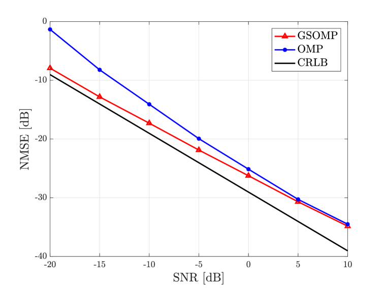
Figure 7: NMSE versus SNR for a user with an $4$-element ULA; $20\times 20$-element UPA, $N_{\text{RF}}=2$, NLoS channel with $L=3$ paths, $S=400$ subcarriers, and super-resolution dictionaries with $G=4N_{B}$ and $G^{u}=4N_{U}$.

VI-A3 Subcarrier Selection

In the previous experiments, we assumed that the GSOMP-based estimator employs all the subcarriers, i.e., $|\mathcal{S}|=400$, to estimate the common support of the channel gain vectors $\{\mathbf{\beta}[s]\}_{s=0}^{S-1}$. However, this might lead to a very high computation burden. Thus, we can employ only a set of successive subcarriers to detect the common support, i.e., steps $2-8$ of Algorithm $2$, and then use this support to estimate the channel at every subcarrier $s\in\mathcal{S}$, which corresponds to step $9$ of Algorithm $2$. We refer to this scheme as GSOMP with subcarrier selection (GSOMP-SS). From Fig. 8, we observe that we can accurately estimate the uplink channel in the moderate SNR regime by employing only a small number of pilot subcarriers in the common support detection steps. Note, though, that using one subcarrier per $50$ pilot subcarriers slightly increases the NMSE in the low SNR regime.

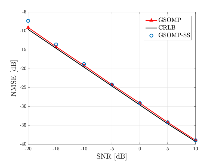
Figure 8: NMSE versus SNR for a single-antenna user. In GSOMP-SS, one pilot subcarrier per $50$ subcarriers is used to detect the common support; $40\times 40$-element UPA, $N_{\text{RF}}=2$, NLoS channel with $L=3$ paths, and $S=400$ subcarriers.

VI-B Hybrid Combining for Single-Antenna Users

VI-B1 Achievable Rate with Perfect CSI

We start the performance assessment of our combiner by considering a LoS channel. In this case, the complex path gain is given by $\beta_{0}(f)=\alpha_{0}(f)e^{-j2\pi f_{c}\tau_{0}}$, where $\tau_{0}=~{}\mathtt{D}/c$ is the ToA of the LoS path, and $\alpha_{0}(f)$ is specified according to (8). For each channel realization, perfect knowledge of the DoA is assumed at the BS, which can be acquired using the GSOMP estimator. We also consider the following cases:

• A fully-digital architecture where the BS employs the frequency-selective combiner $1/\sqrt{N_{B}}\mathbf{a}(\phi_{0},\theta_{0},f)$.

• A hybrid architecture where the BS uses the narrowband combiner $1/\sqrt{N_{B}}\mathbf{a}(\phi_{0},\theta_{0},0)$.

• A hybrid architecture where the proposed combiner (22) is used, with $N_{\text{sb}}=10$ and $M_{\text{sb}}=10$ virtual subarrays.

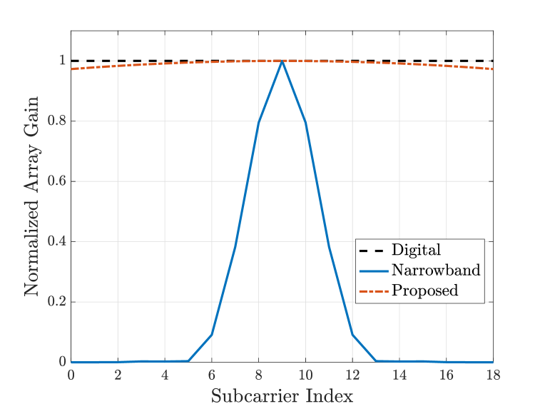
Figure 9: Normalized array gain for an $100\times 100$-element UPA. In the proposed scheme, $N_{\text{sb}}M_{\text{sb}}-1=99$ TTD elements are employed; LoS channel, $(\phi_{0},\theta_{0})=(\pi/4,\pi/3)$, and $S=18$ subcarriers.

The normalized array gain is plotted in Fig. 9, where we see that our combiner atttains approximately the maximum gain over the entire signal bandwidth of $B=40$ GHz. Next, we focus on the average achievable rate, which is calculated as

$$R=\sum_{s=1}^{S}\Delta B\mathbb{E}\left\{\log_{2}\left(1+\frac{P_{d}|\mathbf{f}_{\text{RF}}^{H}\mathbf{h}[s]|^{2}}{\Delta B\sigma^{2}}\right)\right\},$$ (58)

where $P_{d}=P_{t}/S$ is the power per subcarrier, and $\mathbf{f}_{\text{RF}}$ denotes the corresponding combiner.

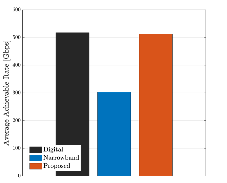
Figure 10: Average achievable rate under perfect CSI for a LoS channel; single-antenna user, $100\times 100$-element UPA, $99$ TTD elements in the proposed scheme, and $S=18$ subcarriers.

The results are given in Fig. 10. Specifically, the achievable rates are $517$ Gbps, $514$ Gbps, and $303$ Gbps for the digital, proposed, and narrowband schemes, respectively. Thus, the proposed combiner performs very close to the fully-digital scheme, while offering a $40\%$ gain with respect to the narrowband combiner. Additionally, this is done by employing only $N_{\text{sb}}M_{\text{sb}}-1=99$ TTD elements for an $100\times 100$-element UPA, which yields an excellent trade-off between hardware complexity and performance. Lastly, note that transmission rates at least $R=0.5$ Tbps at $\mathtt{D}=15$ meters can be achieved through an $100\times 100$-element UPA, which would not be feasible with an equivalent ULA under a footprint constraint.

VI-B2 Achievable Rate with Imperfect CSI

We now evaluate the average achievable rate attained by the proposed combiner along with the GSOMP-based estimator. To this end, we consider a NLoS multi-path channel. The complex path gain of the $l$th NLoS path is $\beta_{l}(f)=\alpha_{l}(f)e^{-j2\pi f_{c}\tau_{l}}$, where $\tau_{l}$ is the ToA, and $\alpha_{l}(f)$ is calculated according to (10) assuming $\phi_{i,l}\sim\mathcal{U}(-\pi/2,\pi/2)$. Under imperfect CSI, the BS treats the channel estimate as the true channel, and combines the received signal with the maximum-ratio combiner $\hat{\mathbf{h}}[s]/\|\hat{\mathbf{h}}[s]\|$. Let $\mathbf{h}[s]=\hat{\mathbf{h}}[s]-\mathbf{e}[s]$, with $\mathbf{e}[s]$ denoting the channel estimation error for the $s$th subcarrier. The combined signal for the $s$th subcarrier is then written as

$$y[s] =\sqrt{P_{d}}\|\hat{\mathbf{h}}[s]\|x[s]-\sqrt{P_{d}}\frac{\hat{\mathbf{h}}^{H}[s]\mathbf{e}[s]}{\|\hat{\mathbf{h}}[s]\|}x[s]+\frac{\hat{\mathbf{h}}^{H}[s]}{\|\hat{\mathbf{h}}[s]\|}\mathbf{n}[s]$$

$$=\sqrt{P_{d}}\|\hat{\mathbf{h}}[s]\|x[s]+n_{\text{eff}}[s],$$ (59)

where $n_{\text{eff}}[s]=(-\sqrt{P_{d}}\hat{\mathbf{h}}^{H}[s]\mathbf{e}[s]x[s]+\hat{\mathbf{h}}^{H}[s]\mathbf{n}[s])/\|\hat{\mathbf{h}}[s]\|$ is the effective noise. Unfortunately, it is challenging to derive an achievable rate of channel model (VI-B2) since the effective noise is correlated with the desired signal. Nevertheless, as shown in the previous numerical results, the channel estimation error is small. Hence, it is reasonably assumed that, conditioned on the channel estimates, the effective noise is uncorrelated with the desired signal. Then, we obtain the following approximation for the equivalent SNR at the $s$th subcarrier [47]

$$\text{SNR}_{\text{eq}}[s]\approx\frac{P_{d}\|\hat{\mathbf{h}}[s]\|^{2}}{\Delta B\sigma^{2}+P_{d}\hat{\mathbf{h}}^{H}[s]\mathbf{R}_{\mathbf{e}[s]}\hat{\mathbf{h}}[s]/\|\hat{\mathbf{h}}[s]\|^{2}},$$ (60)

where $\mathbf{R}_{\mathbf{e}[s]}\triangleq\mathbb{E}\{\mathbf{e}[s]\mathbf{e}^{H}[s]\}$. The corresponding average achievable rate under imperfect CSI is then [47]

$$R\approx\sum_{s=1}^{S}\Delta B\mathbb{E}\left\{\log_{2}\left(1+\text{SINR}_{\text{eq}}[s]\right)\right\}.$$ (61)

A closed-form expression for $\mathbf{R}_{\mathbf{e}[s]}$ can be derived by assuming perfect recovery of the common support of the channel gain vectors. More specifically, from the CRLB analysis, we have that the error $\mathbf{e}[s]\triangleq\bar{\mathbf{A}}_{s}(\mathcal{I})\left(\hat{\bar{\bm{\beta}}}[s]-\tilde{\bar{\bm{\beta}}}[s]\right)$ is distributed as $\mathcal{CN}\left(\mathbf{0},\mathbf{R}_{\mathbf{e}[s]}\right)$, where $\mathbf{R}_{\mathbf{e}[s]}=\bar{\mathbf{A}}_{s}(\mathcal{I})\mathbf{I}^{-1}\left(\tilde{\bar{\bm{\beta}}}[s]\right)\bar{\mathbf{A}}^{H}_{s}(\mathcal{I})$.

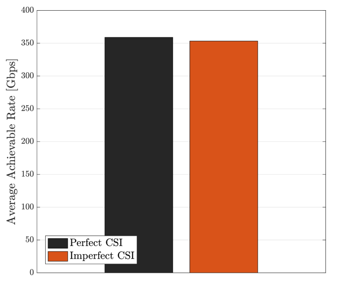
Figure 11: Average achievable rate under imperfect CSI for a NLoS channel with $L=2$ paths; single-antenna user, $100\times 100$-element UPA, $99$ TTD elements per RF chain, and $S=400$ subcarriers.

Figure 11 depicts the average achievable rate under perfect and imperfect CSI. In the imperfect CSI case, the common support of the channel gain vectors is computed by the GSOMP-based estimator. As observed from Fig. 11, the average achievable rate attained by the proposed channel estimator approaches that of the perfect CSI case.

VI-C Hybrid SVD Transmission for Multi-Antenna Users

In this section, we consider a multi-antenna user. As previously shown, we can accurately estimate the channel using the GSOMP-based estimator, and hence perfect CSI is assumed. To have a fair comparison between the single-antenna and multi-antenna user cases, we fix the number of antennas to $N_{U}N_{B}=100\times 100$, and we consider an $100\times 50$-element UPA at the BS and an $2$-element ULA at the user. Due to the small user array size, we assume a fully-digital array at the user, where $N^{u}_{\text{RF}}=N_{U}=2$. Subsequently, we compare the following transmission schemes:

• Digital: the combiner $\mathbf{F}[s]$ and precoder $\mathbf{B}[s]$ are designed using the SVD of the channel $\mathbf{H}[s]$.

• Proposed: the wideband RF combiner $\mathbf{F}_{\text{RF}}[s]$ implements the scaled matrix $1/\sqrt{N_{B}}\mathbf{H}_{B}(f)$, defined in (48), using TTD and virtual array partition. The baseband combiner $\mathbf{F}_{\text{BB}}[s]$ and precoder $\mathbf{B}[s]$ are then designed using the SVD of the effective channel $\mathbf{F}^{H}_{\text{RF}}[s]\mathbf{H}[s]$.

• Narrowband: the frequency-flat RF combiner $\mathbf{F}_{\text{RF}}$ implements the scaled matrix $1/\sqrt{N_{B}}\mathbf{H}_{B}(0)$ defined in (48). The baseband combiner $\mathbf{F}_{\text{BB}}[s]$ and precoder $\mathbf{B}[s]$ are then designed based on the SVD of the effective channel $\mathbf{F}^{H}_{\text{RF}}\mathbf{H}[s]$.

The average achievable rate is calculated as

$$R=\sum_{s=0}^{S-1}\sum_{n=0}^{N^{u}_{\text{RF}}}\Delta B\mathbb{E}\left\{\log_{2}\left(1+\frac{p_{n,s}\sigma^{2}_{n}(\mathbf{F}^{H}[s]\mathbf{H}[s]\mathbf{B}[s])}{\Delta B\sigma^{2}}\right)\right\},$$ (62)

where the set $\{p_{n,s}\}$ of powers is calculated using the waterfilling power allocation algorithm, and $\sigma_{n}(\cdot)$ denotes the $n$th singular value of the input matrix. From Fig. 12, we consolidate that effectiveness of the proposed TTD-based method, which performs close to the fully-digital transmission scheme. More importantly, the deployment of a few antennas at the user side along with waterfilling power allocation boosts the average achievable rate compared to the single-antenna user case, which enables rates much higher than $R=0.5$ Tbps at a distance $\mathtt{D}=15$ m. Another benefit of having multiple user antennas is the reduction of the BS array size, which permits combating the spatial-wideband effect with a small number of TTD elements. In particular, for the $100\times 50$-element UPA under consideration, we have used $N_{\text{sb}}=10$ and $M_{\text{sb}}=5$ virtual subarrays, resulting in $N_{\text{sb}}M_{\text{sb}}-1=49$ TTD elements.

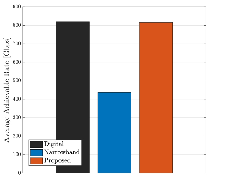
Figure 12: Average achievable rate a for a NLoS channel with $L=2$ paths; multi-antenna user with an $2$-element ULA, $100\times 50$-element UPA, $49$ TTD elements per RF chain, and $S=400$ subcarriers.

VI-D Near-Field Considerations

In the far-field region, the spherical wavefront degenerates to a plane wavefront, which allows the use of the parallel-ray approximation to derive the array response vector (7). Due to the large array aperture of THz massive MIMO, though, near-field considerations are of particular interest. Recall that near-field refers to distances smaller than the Fraunhofer distance $\mathtt{D}_{f}\triangleq 2\mathtt{D}_{\max}^{2}/\lambda$, where $\mathtt{D}_{\max}$ is the maximum dimension of the antenna array, and $\lambda$ is the carrier wavelength. For a UPA with $N=M$, we have $\mathtt{D}_{\max}^{2}=2(N-1)^{2}d^{2}$, i.e., length of its diagonal dimension, which leads to $\mathtt{D}_{f}=(N-1)^{2}\lambda$ for a half-wavelength spacing. Then, for $f_{c}=300$ GHz and an $100\times 100$-element UPA, $\mathtt{D}_{f}\approx 9.8$ meters. As a result, the plane wave assumption may not hold anymore in small distances from the BS [50]. In this case, a spherical wavefront is a more appropriate model [51]. Under this model, the array response matrix, $\mathbf{A}(\phi,\theta,f)\in\mathbb{C}^{M\times N}$, of the BS is defined as

$$[\mathbf{A}(\phi,\theta,f)]_{m,n}\triangleq e^{-j2\pi(f_{c}+f)\frac{\mathtt{D}_{mn}(\phi,\theta)}{c}},$$ (63)

where $\mathtt{D}_{mn}(\phi,\theta)=\left((x-nd)^{2}+(y-md)^{2}+z^{2}\right)^{1/2}$ is the distance between the $(n,m)$th BS antenna and the scatterer with coordinates $(x,y,z)$; $x\triangleq\mathtt{D}\cos\phi\sin\theta$, $y\triangleq\mathtt{D}\sin\phi\sin\theta$, and $z\triangleq\mathtt{D}\cos\theta$, where $\mathtt{D}$ denotes the distance from the $(0,0)$th BS antenna. The array response vector is then obtained as $\mathbf{a}(\phi,\theta,f)=\text{vec}(\mathbf{A}(\phi,\theta,f))$. We now calculate the average achievable rate for the TTD-based combiner (22) under the plane and spherical wave models. The combiner is designed assuming a plane wavefront in both cases. From Fig. 13, a very good match between the two models is observed even for distances smaller than the Fraunhofer distance. Thus, the proposed combiner can be used at near-field distances without incurring a significant rate loss. However, we stress that a comprehensive study of the near-field effects under different array arrangements and sizes is left for future work.

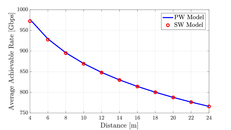
Figure 13: Average achievable rate of the TTD-based wideband combiner for a LoS channel; single-antenna user, and $100\times 100$-element UPA.

VII Conclusions

We have proposed a solution to the channel estimation and hybrid combining problems in wideband THz massive MIMO. Specifically, we first derived the THz channel model with SFW effects for a UPA at the BS and a single-antenna user. We then showed that standard narrowband combining leads to severe reduction of the array gain due to beam squint. To tackle this problem, we introduced a novel TTD-based wideband combiner with a low-complexity implementation due to the virtual subarray rationale. We next proposed a CS algorithm along with a wideband dictionary to acquire reliably the CSI with reduced training overhead under the spatial-wideband effect. To study the performance of the proposed schemes, we derived the CRLB and computed the achievable rate under imperfect CSI. We also extended our analysis to the multi-antenna user case, and conducted numerical results.

Simulations demonstrated that our design provides nearly beam squint-free operation, as well as enables accurate CSI acquisition even in the low SNR regime. Regarding the insights drawn from our study, the deployment of multiple antennas at the user can alleviate the spatial-wideband effect by reducing the BS’ array size, whilst keeping constant the total number of antennas. As a result, the TTD-based wideband array can offer the power gain required to compensate for the very high propagation losses at THz bands. Additionally, in the case of multi-path propagation, it has been shown that SVD-based transmission can boost performance and permit rates more than half terabit per second over a distance of several meters. In conclusion, wideband massive MIMO is expected to be a key enabler for future THz wireless networks.

Regarding future work, it would be interesting to study the performance of wideband THz massive MIMO under hardware impairments, as well as investigate the beam tracking problem in high-mobility scenarios. Moreover, it would be interesting to compare OFDM with SC-FDE, and derive an analytical expression for the PAPR metric.

Appendix A

For the normalized array gain, we have that

$$\frac{|\mathbf{a}^{H}(\phi,\theta,0)\mathbf{a}(\phi,\theta,f)|}{N_{B}}=$$

$$=\frac{|\left(\mathbf{a}_{x}(\phi,\theta,0)^{H}\otimes\mathbf{a}_{y}(\phi,\theta,0)^{H}\right)\left(\mathbf{a}_{x}(\phi,\theta,f)\otimes\mathbf{a}_{y}(\phi,\theta,f)\right)|}{NM}$$

$$=\frac{|\left(\mathbf{a}_{x}(\phi,\theta,0)^{H}\mathbf{a}_{x}(\phi,\theta,f)\right)\left(\mathbf{a}_{y}^{H}(\phi,\theta,0)\mathbf{a}_{y}(\phi,\theta,f)\right)|}{NM}.$$

Then, it holds

$$\frac{|\mathbf{a}_{x}(\phi,\theta,0)^{H}\mathbf{a}_{x}(\phi,\theta,f)|}{N} =\frac{1}{N}\left|\sum_{n=0}^{N-1}e^{-j2\pi fn\frac{d}{c}\sin\theta\cos\phi}\right|$$

$$=\frac{1}{N}\left|\frac{1-e^{-j2\pi fN\frac{d}{c}\sin\theta\cos\phi}}{1-e^{-j2\pi f\frac{d}{c}\sin\theta\cos\phi}}\right|$$

$$=\frac{1}{N}\left|\frac{\sin\left(N\pi f\Delta_{x}\right)}{\sin\left(\pi f\Delta_{x}\right)}\right|$$

$$=D_{N}(2\pi f\Delta_{x}),$$

where $\Delta_{x}=\frac{d}{c}\sin\theta\cos\phi$. Likewise, we get

$$\frac{|\mathbf{a}_{y}(\phi,\theta,0)^{H}\mathbf{a}_{y}(\phi,\theta,f)|}{M}=D_{M}(2\pi f\Delta_{y}),$$

where $\Delta_{y}=\frac{d}{c}\sin\theta\sin\phi$, which yields the desired result.

Appendix B

Using the identity $\mathbf{a}_{x}\otimes\mathbf{a}_{y}=\text{vec}\left(\mathbf{a}_{y}\mathbf{a}^{T}_{x}\right)$, we have

$$\mathbf{A}(\phi,\theta,f)\triangleq\mathbf{a}_{y}(\phi,\theta,f)\mathbf{a}^{T}_{x}(\phi,\theta,f)$$

$$=\begin{bmatrix}\mathbf{a}_{y,1}(\phi,\theta,f)\\ \vdots\\ \mathbf{a}_{y,M_{\text{sb}}}(\phi,\theta,f)\end{bmatrix}\left[\mathbf{a}^{T}_{x,1}(\phi,\theta,f),\cdots,\mathbf{a}^{T}_{x,N_{\text{sb}}}(\phi,\theta,f)\right]$$

$$=\begin{bmatrix}\mathbf{A}_{11}(\phi,\theta,f)&\cdots&\mathbf{A}_{1N_{\text{sb}}}(\phi,\theta,f)\\ \mathbf{A}_{21}(\phi,\theta,f)&\cdots&\mathbf{A}_{1N_{\text{sb}}}(\phi,\theta,f)\\ \vdots&\ddots&\vdots\\ \mathbf{A}_{M_{\text{sb}}1}(\phi,\theta,f)&\cdots&\mathbf{A}_{M_{\text{sb}}N_{\text{sb}}}(\phi,\theta,f)\end{bmatrix},$$ (64)

where $\mathbf{A}_{mn}(\phi,\theta,f)\triangleq\mathbf{a}_{y,m}(\phi,\theta,f)\mathbf{a}^{T}_{x,n}(\phi,\theta,f)$. We also have that

$$\mathbf{A}_{mn}(\phi,\theta,f)=\mathbf{a}_{y,m}(\phi,\theta,f)\mathbf{a}^{T}_{x,n}(\phi,\theta,f)\\ =e^{-j2\pi(n-1)\tilde{N}(f_{c}+f)\Delta_{x}-j2\pi(m-1)\tilde{M}(f_{c}+f)\Delta_{y}}\mathbf{A}_{11}(\phi,\theta,f).$$ (65)

Using the above relationships, we can write

$$\mathbf{A}(\phi,\theta,0)\odot\mathbf{T}[s]=\mathbf{v}_{y}\mathbf{v}_{x}^{T},$$ (66)

where

$$\mathbf{v}_{x}=\left[e^{-j2\pi(n-1)\tilde{N}(f_{c}+f)\Delta_{x}}\mathbf{a}_{x,1}(\phi,\theta,0)\right]_{n=1}^{N_{\text{sb}}},$$ (67)

and

$$\mathbf{v}_{y}=\left[e^{-j2\pi(m-1)\tilde{M}(f_{c}+f)\Delta_{y}}\mathbf{a}_{y,1}(\phi,\theta,0)\right]_{m=1}^{M_{\text{sb}}}.$$ (68)

Now consider a path with array response $\mathbf{a}^{H}(\phi,\theta,f)$. Then,

$$\mathbf{f}^{H}_{\text{RF}}\mathbf{a}(\phi,\theta,f)=$$

$$=\frac{1}{\sqrt{N_{B}}}\text{vec}^{H}(\mathbf{A}(\phi,\theta,0)\odot\mathbf{T}[s])\mathbf{a}(\phi,\theta,f)$$

$$=\frac{\sqrt{N_{B}}}{N_{B}}\left(\mathbf{v}^{H}_{x}\otimes\mathbf{v}^{H}_{y}\right)\left(\mathbf{a}_{x}(\phi,\theta,f)\otimes\mathbf{a}_{y}(\phi,\theta,f)\right)$$

$$=\frac{\sqrt{N_{B}}}{N_{B}}\left(\mathbf{v}^{H}_{x}\mathbf{a}_{x}(\phi,\theta,f)\right)\left(\mathbf{v}^{H}_{y}\mathbf{a}_{y}(\phi,\theta,f)\right)$$

$$=\sqrt{N_{B}}\frac{\mathbf{a}^{H}_{x,1}(\phi,\theta,0)\mathbf{a}_{x,1}(\phi,\theta,f)}{\tilde{N}}\frac{\mathbf{a}^{H}_{y,1}(\phi,\theta,0)\mathbf{a}_{y,1}(\phi,\theta,f)}{\tilde{M}}.$$

As a result, we obtain (23) in Proposition 1.

References

- [1] T. S. Rappaport et al., “Wireless communications and applications above 100 GHz: opportunities and challenges for 6G and beyond,” IEEE Access, vol. 7, pp. 78729-78757, 2019.
- [2] T. Kurner, “Towards future THz communications systems,” Terahertz Sci. Technol., vol. 5, no. 1, pp. 11–17, 2012.
- [3] J. Zhang et al., “Prospective multiple antenna technologies for beyond 5G,” IEEE J. Sel. Areas Commun., vol. 38, no. 8, pp. 1637–1660, Aug. 2020.
- [4] H. J. Song and T. Nagatsuma, “Present and future of terahertz communications,” IEEE Trans. THz Sci. Technol., vol. 1, no. 1, pp. 256–263, Sep. 2011.
- [5] B. Wang, F. Gao, S. Jin, H. Lin, and G. Y. Li, “Spatial- and frequency-wideband effects in millimeter wave massive MIMO systems,” IEEE Trans. Signal Process., vol. 66, no. 13, pp. 3393-3406, Jul. 2018.
- [6] B. Wang et al., “Spatial-wideband effect in massive MIMO with application in mmWave systems,” IEEE Commun. Mag., vol. 56, no. 12, pp. 134-141, Dec. 2018.
- [7] R. J. Mailloux, Phased Array Antenna Handbook. Norwood, MA, USA: Artech House, 2005.
- [8] B. Peng, S. Wesemann, K. Guan, W. Templ, and T. Kürner, “Precoding and detection for broadband single carrier terahertz massive MIMO systems using LSQR algorithm,” IEEE Trans. Wireless Commun., vol. 18, no. 2, pp. 1026-1040, Feb. 2019.
- [9] F. Sohrabi and W. Yu, “Hybrid analog and digital beamforming for mmWave OFDM large-scale antenna arrays,” IEEE J. Sel. Areas Commun., vol. 35, no. 7, pp. 1432-1443, July 2017.
- [10] J. P. González-Coma, W. Utschick, and L. Castedo, “Hybrid LISA for wideband multiuser millimeter-wave communication systems under beam squint,” IEEE Trans. Wireless Commun., vol. 18, no. 2, pp. 1277-1288, Feb. 2019.
- [11] S. Park, A. Alkhateeb, and R. W. Heath, Jr., “Dynamic subarrays for hybrid precoding in wideband mmwave MIMO systems,” IEEE Trans. Wireless Commun., vol. 16, no. 5, pp. 2907–2920, May 2017.
- [12] L. Kong, S. Han, and C. Yang, “Hybrid precoding with rate and coverage constraints for wideband massive MIMO systems,” IEEE Trans. Wireless Commun., vol. 17, no. 7, pp. 4634–4647, July 2018.
- [13] M. Cai et al, “Effect of wideband beam squint on codebook design in phased-array wireless systems,” in Proc. IEEE GLOBECOM, Dec. 2016.
- [14] X. Liu and D. Qiao, “Space-time block coding-based beamforming for beam squint compensation,” IEEE Wireless Commun. Lett., vol. 8, no. 1, pp. 241–244, Feb. 2019.
- [15] C. Lin, G. Y. Li, and L. Wang, “Subarray-based coordinated beamforming training for mmWave and sub-THz communications,” IEEE J. Sel. Areas Commun., vol. 35, no. 9, pp. 2115-2126, Sept. 2017.
- [16] H. Hashemi, T. Chu, and J. Roderick, “Integrated true-time-delay-based ultra-wideband array processing,” IEEE Commun. Mag., vol. 46, no. 9, pp. 162–172, Sep. 2008.
- [17] J. Tan and L. Dai, “Delay-phase precoding for THz massive MIMO with beam split,” in Proc. IEEE GLOBECOM, Dec. 2019.
- [18] B. Wang, X. Li, F. Gao, and G. Y. Li, “Power leakage elimination for wideband mmWave massive MIMO-OFDM systems: An energy-focusing window approach,” IEEE Trans. Signal Process., vol. 67, no. 21, pp. 5479-5494, Nov. 2019.
- [19] J. P. González-Coma, J. Rodríguez-Fernández, N. González-Prelcic, L. Castedo, and R. W. Heath, Jr., “Channel estimation and hybrid precoding for frequency selective multiuser mmWave MIMO systems,” IEEE J. Sel. Topics Signal Process., vol. 12, no. 2, pp. 353-367, May 2018.
- [20] C. Lin and G. Y. Li, “Indoor terahertz communications: How many antenna arrays are needed?,” IEEE Trans. Wireless Commun., vol. 14, no. 6, pp. 3097-3107, June 2015.
- [21] H. Sarieddeen, M. S. Alouini, and T. Y. Al-Naffouri, “Terahertz-band ultra-massive spatial modulation MIMO,” IEEE J. Sel. Areas Commun., vol. 37, no. 9, pp. 2040-2052, Sept. 2019.
- [22] Q. Ma, D. M. W. Leenaerts, and P. G. M. Baltus, “Silicon-based true-time-delay phased array front-ends at Ka-band,” IEEE Trans. Microw. Theory Techn., vol. 63, no. 9, pp. 2942–2952, Sep. 2015.
- [23] C. Han and Y. Chen, “Propagation modeling for wireless communications in the terahertz band,” IEEE Commun. Mag., vol. 56, no. 6, pp. 96-101, June 2018.
- [24] C. A. Balanis, Antenna Theory: Analysis and Design, John Wiley & Sons, 2012.
- [25] D. Tse and P. Viswanath, Fundamentals of Wireless Communication. New York, NY, USA: Cambridge Univ. Press, 2005.
- [26] A. F. Molisch, “Ultrawideband propagation channels-theory, measurement, and modeling,” IEEE Trans. Veh. Technol., vol. 54, no. 5, pp. 1528-1545, Sept. 2005.
- [27] A. A. Boulogeorgos, E. N. Papasotiriou, and A. Alexiou, “Analytical performance assessment of THz wireless systems,” IEEE Access, vol. 7, pp. 11436-11453, 2019.
- [28] C. Han, A. O. Bicen, and I. F. Akyildiz, “Multi-ray channel modeling and wideband characterization for wireless communications in the terahertz band,” IEEE Trans. Wireless Commun., vol. 14, no. 5, pp. 2402–2412, May 2015.
- [29] R. Piesiewicz et al., “Scattering analysis for the modeling of THz communication systems,” IEEE Trans. Antennas Propag., vol. 55, no. 11, pp. 3002–3009, Nov. 2007.
- [30] C. Lin and G. Y. Li, “Adaptive beamforming with resource allocation for distance-aware multi-user indoor terahertz communications,” IEEE Trans. Commun., vol. 63, no. 8, pp. 2985-2995, Aug. 2015.
- [31] O. E. Ayach, R. W. Heath, Jr., S. Abu-Surra, S. Rajagopal, and Z. Pi, “The capacity optimality of beam steering in large millimeter wave MIMO systems,” in Proc. IEEE SPAWC, June 2012, pp. 100-104.
- [32] S. M. Perera, A. Madanayake, and R. J. Cintra, “Radix-2 self-recursive sparse factorizations of delay Vandermonde matrices for wideband multi-beam antenna arrays,” IEEE Access, vol. 8, pp. 25498-25508, 2020.
- [33] W. U. Bajwa, J. Haupt, A. M. Sayeed, and R. Nowak, “Compressed channel sensing: a new approach to estimating sparse multipath channels,” Proc. IEEE, vol. 98, no. 6, pp. 1058-1076, June 2010.
- [34] R. Méndez-Rial, C. Rusu, N. González-Prelcic, A. Alkhateeb, and R. W. Heath, Jr., “Hybrid MIMO architectures for millimeter wave communications: Phase shifters or switches?,” IEEE Access, vol. 4, pp. 247-267, 2016.
- [35] R. W. Heath, Jr., N. González-Prelcic, S. Rangan, W. Roh, and A. M. Sayeed, “An overview of signal processing techniques for millimeter wave MIMO systems,” IEEE J. Sel. Topics Signal Process., vol. 10, no. 3, pp. 436-453, Apr. 2016.
- [36] T. T. Cai and L. Wang, “Orthogonal matching pursuit for sparse signal recovery with noise,” IEEE Trans. Inf. Theory, vol. 57, no. 7, pp. 4680-4688, July 2011.
- [37] L. Harry and V. Trees, Optimum Array Processing: Detection, Estimation, and Modulation Theory. John Wiley & Sons, 2002.
- [38] A. M. Sayeed, “Deconstructing multi-antenna fading channels,” IEEE Trans. Signal Process., vol. 50, no. 10, pp. 2563–2579, Oct. 2002.
- [39] H. Xie, F. Gao, S. Zhang, and S. Jin, “A unified transmission strategy for TDD/FDD massive MIMO systems with spatial basis expansion model,” IEEE Trans. Veh. Technol., vol. 66, no. 4, pp. 3170-3184, Apr. 2017.
- [40] Z. Gao, L. Dai, Z. Wang, and S. Chen, “Spatially common sparsity based adaptive channel estimation and feedback for FDD massive MIMO,” IEEE Trans. Signal Process., vol. 63, no. 23, pp. 6169-6183, Dec. 2015.
- [41] J. A. Tropp, A. C. Gilbert, and M. J. Strauss, “Algorithms for simultaneous sparse approximation—part I: Greedy pursuit,” Signal Process., vol. 86, no. 3, pp. 572–588, 2006.
- [42] J. A. Tropp and A. C. Gilbert, “Signal recovery from random measurements via orthogonal matching pursuit,” IEEE Trans. Inf. Theory, vol. 53, no. 12, pp. 4655–4666, Dec. 2007.
- [43] S. M. Kay, Fundamentals of Statistical Processing: Estimation Theory, vol. 1. Upper Saddle River, NJ, USA: Prentice-Hall, 1993.
- [44] J. Lee, G. Gil, and Y. H. Lee, “Exploiting spatial sparsity for estimating channels of hybrid MIMO systems in millimeter wave communications,” in Proc. IEEE GLOBECOM, Dec. 2014, pp. 3326-3331.
- [45] Y. You, L. Zhang, and M. Liu, “IP aided OMP based channel estimation for millimeter wave massive MIMO communication,” in Proc. IEEE WCNC, Apr. 2019.
- [46] J. Lee, G. Gil, and Y. H. Lee, “Channel estimation via orthogonal matching pursuit for hybrid MIMO systems in millimeter wave communications,” IEEE Trans. Commun., vol. 64, no. 6, pp. 2370-2386, June 2016.
- [47] T. L. Marzetta, E. G. Larsson, H. Yang, and H. Q. Ngo, Fundamentals of Massive MIMO. Cambridge, UK: Cambridge University Press, 2016.
- [48] Q. Nadeem, A. Kammoun, and M. Alouini, “Elevation beamforming with full dimension MIMO architectures in 5G systems: A tutorial,” IEEE Commun. Surveys Tuts., vol. 21, no. 4, pp. 3238-3273, Jul. 2019.
- [49] O. E. Ayach, S. Rajagopal, S. A.-Surra, Z. Pi, and R. W. Heath, Jr., “Spatially sparse precoding in millimeter wave MIMO systems,” IEEE Trans. Wireless Commun., vol. 13, no. 3, pp. 1499-1513, Mar. 2014.
- [50] M. Matthaiou, P. de Kerret, G. K. Karagiannidis, and J. A. Nossek, “Mutual information statistics and beamforming performance analysis of optimized LoS MIMO systems,” IEEE Trans. Commun., vol. 58, no. 11, pp. 3316-3329, Nov. 2010.
- [51] F. Bøhagen, P. Orten, and G. E. Øien, “On spherical vs. plane wave modeling of line-of-sight MIMO channels,” IEEE Trans. Commun., vol. 57, no. 3, pp. 841-849, Mar. 2009.