Structural Information Preserving for Graph-to-Text Generation

Abstract

The task of graph-to-text generation aims at producing sentences that preserve the meaning of input graphs. As a crucial defect, the current state-of-the-art models may mess up or even drop the core structural information of input graphs when generating outputs. We propose to tackle this problem by leveraging richer training signals that can guide our model for preserving input information. In particular, we introduce two types of autoencoding losses, each individually focusing on different aspects (a.k.a. views) of input graphs. The losses are then back-propagated to better calibrate our model via multi-task training. Experiments on two benchmarks for graph-to-text generation show the effectiveness of our approach over a state-of-the-art baseline. Our code is available at http://github.com/Soistesimmer/AMR-multiview.

1 Introduction

Many text generation tasks take graph structures as their inputs, such as Abstract Meaning Representation (AMR) (Banarescu et al., 2013), Knowledge Graph (KG) and database tables. For example, as shown in Figure 1(a), AMR-to-text generation is to generate a sentence that preserves the meaning of an input AMR graph, which is composed by a set of concepts (such as “boy” and “want-01”) and their relations (such as “:ARG0” and “:ARG1”). Similarly, as shown in Figure 1(b), KG-to-text generation is to produce a sentence representing a KG, which contains worldwide factoid information of entities (such as “Australia” and “Above the Veil”) and their relations (such as “followedBy”).

Recent efforts on graph-to-text generation tasks mainly focus on how to effectively represent input graphs, so that an attention mechanism can better transfer input knowledge to the decoder when generating sentences. Taking AMR-to-text generation as an example, different graph neural networks (GNNs) (Beck et al., 2018; Song et al., 2018; Guo et al., 2019; Ribeiro et al., 2019) have been introduced to better represent input AMRs than a sequence-to-sequence model (Konstas et al., 2017), and later work (Zhu et al., 2019; Cai and Lam, 2019; Wang et al., 2020) showed that relation-aware Transformers can achieve even better results than GNNs. These advances for encoding have largely pushed the state-of-the-art performance.

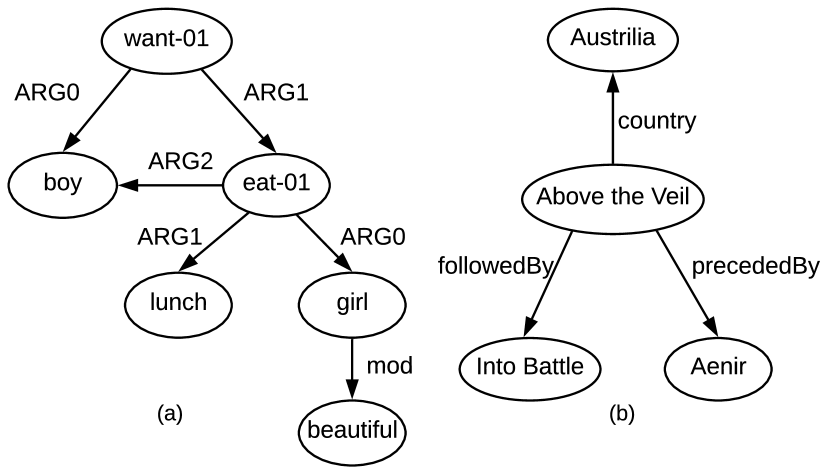
Figure 1: (a) An AMR graph meaning “The boy wants the beautiful girl to eat lunch with him.”, and (b) A knowledge graph carrying the meaning “Above the Veil is an Australian novel and the sequel to Aenir. It was followed by Into the Battle.”

Existing models are optimized by maximizing the conditional word probabilities of a reference sentence, a common signal for training language models. As a result, these models can learn to produce fluent sentences, but some crucial input concepts and relations may be messed up or even dropped. Taking the AMR in Figure 1(a) as an example, a model may produce “the girl wants the boy to go”, which conveys an opposite meaning to the AMR graph. In particular, this can be very likely if “the girl wants” appears much more frequent than “the boy wants” in the training corpus. This is a very important issue, because of its wide existence across many neural graph-to-text generation models, hindering the usability of these models for real-world applications (Dušek et al., 2018, 2019; Balakrishnan et al., 2019).

A potential solution for this issue is improving the training signal to enhance preserving of structural information. However, little work has been done to explore this direction so far, probably because designing such signals is non-trivial. As a first step towards this goal, we propose to enrich the training signal with additional autoencoding losses (Rei, 2017). Standard autoencoding for graph-to-sequence tasks requires reconstructing (parsing into) input graphs, while the parsing algorithm for one type of graphs (such as knowledge graphs) may not generalize to other graph types or may not even exist. To make our approach general across different types of graphs, we propose to reconstruct different views of each input graph (rather than the original graph), where each view highlights one aspect of the graph and is easy to produce. Then through multi-task learning, the autoencoding losses of all views are back-propagated to the whole model so that the model can better follow the input semantic constraints.

Specifically, we break each input graph into a set of triples to form our first view, where each triple (such as “want-01 :ARG0 boy” in Figure 1(a)) contains a pair of entities and their relation. As the next step, the alignments between graph nodes and target words are generated to ground this view into the target sentence for reconstruction. Our second view is the linearization of each input graph produced by depth-first graph traversal, and this view is reconstructed token-by-token from the last decoder state. Overall the first view highlights the local information of each triple relation, the second view focuses on the global semantic information of the entire graph.

Experiments on AMR-to-text generation and WebNLG (Gardent et al., 2017) show that our graph-based multi-view autoencoding loss improves the performance of a state-of-the-art baseline by more than 2 BLEU points without introducing any parameter during decoding. Besides, human studies show that our approach is indeed beneficial for preserving more concepts and relations from input graphs.

2 Related Work

Previous work for neural graph-to-text generation (Konstas et al., 2017; Song et al., 2018; Beck et al., 2018; Trisedya et al., 2018; Marcheggiani and Perez-Beltrachini, 2018; Xu et al., 2018; Cao and Clark, 2019; Damonte and Cohen, 2019; Hajdik et al., 2019; Koncel-Kedziorski et al., 2019; Hong et al., 2019; Song et al., 2019; Su et al., 2017) mainly studied how to effectively represent input graphs, and all these models are trained only with the standard language modeling loss. As the most similar one to our work, Tu et al. (2017) proposed an encoder-decoder-reconstructor model for machine translation, which is trained not only to translate each source sentence into its target reference, but also to translate the target reference back into the source text (reconstruction). Wiseman et al. (2017) extended the reconstruction loss of Tu et al. (2017) on table-to-text generation, where a table contains multiple records that fit into several fields.We study a more challenging topic on how to reconstruct a complex graph structure rather than a sentence or a table, and we propose two general and effective methods that reconstruct different complementary views of each input graph. Besides, we propose methods to breakdown the whole (graph, sentence) pair into smaller pieces of (edge, word) pairs with alignments, before training our model to reconstruct each edge given the corresponding word. On the other hand, neither of the previous efforts tried to leverage this valuable information.

Our work is remotely related to the previous efforts on string-to-tree neural machine translation (NMT) (Aharoni and Goldberg, 2017; Wu et al., 2017; Wang et al., 2018), which aims at generating target sentences with their syntactic trees. One major difference is that their goal is producing grammatical outputs, while ours is preserving input structures. Besides, our multi-view reconstruction framework is a detachable component on top of the decoder states for training, so no extra error propagation (for structure prediction) can be introduced. Conversely, their models generate trees together with target sentences, thus extra efforts (Wu et al., 2017) are introduced to alleviate error propagation. Finally, there exist transition-based algorithms (Nivre, 2003) to convert tree parsing into the prediction of transition actions, while we study reconstructing graphs, where there is no common parsing algorithm for all graph types.

Autoencoding loss by input reconstruction was mainly adopted on sequence labeling tasks, such as named entity recognition (NER) (Rei, 2017; Liu et al., 2018a; Jia et al., 2019), simile detection (Liu et al., 2018b) and sentiment analysis (Rei and Søgaard, 2019). Since input reconstruction is not intuitively related to these tasks, the autoencoding loss only serves as more training signals. Different from these efforts, we leverage autoencoding loss as a means to preserve input knowledge. Besides, we study reconstructing complex graphs, proposing a general multi-view approach for this goal.

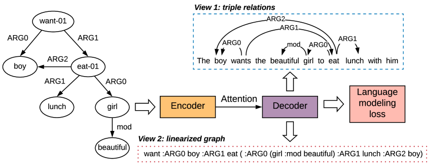
Figure 2: The training framework using multi-view autoencoding losses.

3 Base: Structure-Aware Transformer

Formally, an input for graph-to-text generation can be represented as $\boldsymbol{G}=\langle\boldsymbol{V},\boldsymbol{E}\rangle$, where $\boldsymbol{V}$ is the set of graph nodes and $\boldsymbol{E}$ corresponds to all graph edges. Each edge $e\in\boldsymbol{E}$ is a triple $(v_{i},l,v_{j})$, showing labelled relation between two connected nodes $v_{i}$ and $v_{j}$. Given a graph, we choose a recent relation-aware transformer model (Zhu et al., 2019) as our baseline to generate the ground-truth sentence $\boldsymbol{y}=(y_{1},\dots,y_{N})$ that contain the same meaning as the input graph. It exhibits the state-of-the-art performance for AMR-to-text generation.

3.1 Structure-aware Transformer Encoder

Similar to the standard model (Vaswani et al., 2017), the structure-aware Transformer encoder stacks multiple self-attention layers on top of an embedding layer to encode linearized graph nodes. Taking the $l$-th layer for example, it consumes the states of its preceding layer ($\boldsymbol{h}_{1}^{l-1}\dots\boldsymbol{h}_{N}^{l-1}$, or the embedding layer when $l$ is 1) and its states are then updated by a weighted sum:

$$\boldsymbol{h}_{i}^{l}=\sum_{j\in[1..N]}\alpha_{ij}(\boldsymbol{h}_{j}^{l-1}\boldsymbol{W}^{P}+\boldsymbol{\gamma}_{ij}\boldsymbol{W}^{R_{1}})\text{,}$$ (1)

where $\boldsymbol{\gamma}_{ij}$ is the vector representation of the relation between nodes $v_{i}$ and $v_{j}$, and $\boldsymbol{W}^{P}$ and $\boldsymbol{W}^{R_{1}}$ are model parameters. The weights, such as $\alpha_{ij}$, are obtained by relation-aware self-attention:

$$\alpha_{ij} =\frac{\exp(e_{ij})}{\sum_{k\in[1..N]}\exp(e_{ik})}$$ (2)

$$e_{ij} =\frac{\big{(}\boldsymbol{h}_{i}^{l-1}\boldsymbol{W}^{Q}\big{)}\big{(}\boldsymbol{h}_{j}^{l-1}\boldsymbol{W}^{K}+\boldsymbol{\gamma}_{ij}\boldsymbol{W}^{R_{2}}\big{)}^{\intercal}}{\sqrt{d_{h}}}$$ (3)

where $\boldsymbol{W}^{Q}$, $\boldsymbol{W}^{K}$ and $\boldsymbol{W}^{R_{2}}$ are model parameters, and $d_{h}$ denotes the encoder-state dimension. The encoder adopts $L$ self-attention layers and $\boldsymbol{H}^{L}=$ $(\boldsymbol{h}_{1}^{L}\dots\boldsymbol{h}_{|\boldsymbol{V}|}^{L})$ represents the concatenated top-layer hidden states of the encoder, which will be used in attention-based decoding.

Compared with the standard model, this encoder introduces the vectorized structural information (such as $\boldsymbol{\gamma}_{ij}$) for all node pairs. Given a node pair $v_{i}$ and $v_{j}$, generating such information involves two main steps. First, a sequence of graph edge labels along the path from $v_{i}$ to $v_{j}$ are obtained, where a direction symbol is added to each label to distinguish the edge direction. For instance, the label sequence from “boy” to “girl” in Figure 1(a) is “:ARG0$\uparrow$ :ARG1$\downarrow$ :ARG0$\downarrow$”. As the next step, the label sequence is treated as a single (feature) token and represented by the corresponding embedding vector, and this vector is taken as the vectorized structural information $\boldsymbol{\gamma}_{ij}$ from $v_{i}$ to $v_{j}$. Since there are a large number of features, only the most frequent 20K are kept, while the rest are mapped into a special UNK feature.

3.2 Standard Transformer Decoder

The decoder is the same as the standard Transformer architecture, which stacks an embedding layer, multiple ($L$) self-attention layers and a linear layer with softmax activation to generate target sentences in a word-by-word manner. Each target word $y_{i}$ and decoder state $\boldsymbol{s}_{i}$ are generated sequentially by the self-attention decoder:

$$y_{i},\boldsymbol{s}_{i}=\mathtt{SADecoder}([\boldsymbol{H}^{L};\boldsymbol{s}_{1}...\boldsymbol{s}_{i-1}],y_{i-1})\text{,}$$ (4)

where $\mathtt{SADecoder()}$ is the function of decoding one step with the self-attention-based decoder.

3.3 Training with Language Modeling Loss

Same as most previous work, this model is trained with the standard language modeling loss that minimizes the negative log-likelihood of conditional word probabilities:

$$\begin{split}l_{base}&=-\sum_{i\in[1..N]}\log p(y_{i}|y_{1},...,y_{i-1};\boldsymbol{G})\\ &=-\sum_{i\in[1..N]}p(y_{i}|\boldsymbol{s}_{i};\boldsymbol{\theta})\text{,}\end{split}$$ (5)

where $\boldsymbol{\theta}$ represents all model parameters.

4 Multi-View Autoencoding Losses

Figure 2 visualizes the training framework using our multi-view autoencoding losses, where the attention-based encoder-decoder model with the language modeling loss is the baseline. Our losses are produced by reconstructing the two proposed views (surrounded by slashed or dotted box) of the input graph, where each view represents a different aspect of the input. With the proposed losses, we expect to better refine our model for preserving the structural information of input graphs.

4.1 Loss 1: Reconstructing Triple Relations with Biaffine Attention

Our first view breaks each input graph into a set of triples, where each triple (such as “want-01 :ARG0 boy” in Figure 1(a)) contains a pair of nodes and their labeled relation. Next, we use pre-generated alignments between graph nodes and target words to ground the graph triples onto the target sentence. As illustrated in the slashed blue box of Figure 2, the result contains several labeled arcs, each connecting a word pair (such as “wants” and “boy”). While each arc represents a local relation, their combination implies the global input structure.

For certain types of graphs, a node can have multiple words. To deal with this situation, we use the first word of both associated graph nodes when grounding a graph edge onto the target sentence. Next, we also connect the first word of each grounded entity with the other words of the entity in order to represent the whole-entity information in the sentence. Taking the edge “followedBy” in Figure 1(b) as an example, we first ground it onto the target sentence to connect words “Above” and “Into”. Next, we create edges with label “compound” from “Above” to words “the” and “Veil”, and from “Into” to words “the” and “Battle” to indicate the two associated entity mentions.

For many tasks on graph-to-text generation, the node-to-word alignments can be easily generated from off-the-shell toolkits. For example, in AMR-to-text generation, there have been several aligners (Pourdamghani et al., 2014; Flanigan et al., 2016; Wang and Xue, 2017; Liu et al., 2018c; Szubert et al., 2018) available for linking AMR nodes to words. For knowledge graphs, the alignments can be produced by simple rule-based matching or an entity-linking system.

The resulting structure with labeled arcs connecting word pairs resembles a dependency tree, and thus we employ a deep biaffine model (Dozat and Manning, 2017) to predict this structure from the decoder states. More specifically, the model factorizes the probability for making each arc into two parts: an unlabeled factor and a labeled one. Given the decoder states $\boldsymbol{s}_{1},\dots,\boldsymbol{s}_{N}$, the representation for each word $y_{i}$ as the head or the modifier of any unlabeled factor is calculated by passing its hidden state $\boldsymbol{s}_{i}$ through the corresponding multi-layer perceptrons (MLPs):

$$\boldsymbol{r}_{i}^{\mathrm{arc-h}} =\mathtt{MLP}^{\mathrm{arc-head}}(\boldsymbol{s}_{i})$$ (6)

$$\boldsymbol{r}_{i}^{\mathrm{arc-m}} =\mathtt{MLP}^{\mathrm{arc-mod}}(\boldsymbol{s}_{i})\text{,}$$ (7)

The (unnormalized) scores for the unlabeled factors with any possible head word given the modifier $y_{i}$ are calculated as:

$$\boldsymbol{\phi}_{i}^{\mathrm{arc}}=\boldsymbol{R}^{\mathrm{arc-h}}\boldsymbol{U}_{a}^{\intercal}\boldsymbol{r}_{i}^{\mathrm{arc-m}}+\boldsymbol{R}^{\mathrm{arc-h}}\boldsymbol{v}_{a}\text{,}$$ (8)

where $\boldsymbol{R}^{\mathrm{arc-h}}$ is the concatenation of all $\boldsymbol{r}_{i}^{\mathrm{arc-h}}$, and $\boldsymbol{U}_{a}$ and $\boldsymbol{v}_{a}$ are model parameters. Similarly, the representations for word $y_{i}$ being the head or the modifier of a labeled factor are calculated by two additional MLPs:

$$\boldsymbol{r}_{i}^{\mathrm{label-h}} =\mathtt{MLP}^{\mathrm{label-head}}(\boldsymbol{s}_{i})$$ (9)

$$\boldsymbol{r}_{i}^{\mathrm{label-m}} =\mathtt{MLP}^{\mathrm{label-mod}}(\boldsymbol{s}_{i})\text{,}$$ (10)

and the (unnormalized) scores for all relation labels given the head word $y_{j}$ and the modifier $y_{i}$ are calculated as:

$$\boldsymbol{\phi}_{i,j}^{\mathrm{label}}=\boldsymbol{r}_{j}^{\mathrm{label-h}}\boldsymbol{U}_{l}\boldsymbol{r}_{i}^{\mathrm{label-m}}+\\ (\boldsymbol{r}_{j}^{\mathrm{label-h}}\oplus\boldsymbol{r}_{i}^{\mathrm{label-m}})^{\intercal}\boldsymbol{V}_{l}+\boldsymbol{b}_{l},$$ (11)

where $\boldsymbol{U}_{l}$, $\boldsymbol{V}_{l}$ and $\boldsymbol{b}_{l}$ are model parameters. The overall conditional probability of a labeled arc with label $l$, head word $y_{j}$ and modifier $y_{i}$ is calculated by the following chain rule:

$$p(y_{j},l|y_{i})=p(l|y_{j},y_{i})\cdot p(y_{j}|y_{i})\\ =\mathtt{softmax}(\boldsymbol{\phi}_{i,j}^{\mathrm{label}})_{[l]}\cdot\mathtt{softmax}(\boldsymbol{\phi}_{i}^{\mathrm{arc}})_{[j]},$$ (12)

where $[x]$ in the subscript represents choosing the $x$-th item from the corresponding vector.

As the final step, the loss for reconstructing this view is defined as the negative log-likelihood of all target arcs $\boldsymbol{E}^{\prime}$ (the grounded triples from $\boldsymbol{E}$):

$$l_{auto1}=\sum_{(y_{j},l,y_{i})\in\boldsymbol{E}^{\prime}}-\log p(y_{j},l|y_{i})$$ (13)

4.2 Loss 2: Reconstructing Linearized Graphs with a Transformer Decoder

As a supplement to our first loss for reconstructing the local information of each grounded triple, we introduce the second loss for predicting the whole graph as a linearized sequence. To minimize the loss of the graph structural information caused by linearization, we adopt an algorithm based on depth-first traversal (Konstas et al., 2017), which inserts brackets to preserve graph scopes. One linearized AMR graph is shown in the red dotted box of Figure 2, where the node suffixes (such as “-01”) representing word senses are removed.

One may argue that we could directly predict the original graph so that no structural information would be lost. However, each type of graphs can have their own parsing algorithm due to their unique properties (such as directed vs undirected, rooted vs unrooted, etc). Such an exact prediction will hurt the generality of the proposed approach. Conversely, our solution is general, as linearization works for most types of graphs. From Figure 2 we can observe that the inserted brackets clearly infer the original graph structure. Besides, previous work (Iyer et al., 2017; Konstas et al., 2017) has shown the effectiveness of generating linearized graphs as sequences for graph parsing, which also confirms our observation.

Given a linearized graph represented as a sequence of tokens $x_{1},\dots,x_{M}$, where each token $x_{i}$ can be a graph node, a edge label or a inserted bracket, we adopt another standard Transformer decoder ($\mathtt{SADecoder}_{g}$) to produce the sequence:

$$x_{i},\boldsymbol{t}_{i}=\mathtt{SADecoder}_{g}([\boldsymbol{S};\boldsymbol{t}_{1}...\boldsymbol{t}_{i-1}],x_{i-1})\text{,}$$ (14)

where $\boldsymbol{S}=(\boldsymbol{s}_{1}\dots\boldsymbol{s}_{N})$ denotes the concatenated states for the target sentence (Equation 4), and the loss for reconstructing this view is defined as the negative log-likelihood for the linearized graph:

$$l_{auto2}=-\sum_{i\in[1..M]}\log p(x_{i}|\boldsymbol{t}_{i};\boldsymbol{\theta})\text{,}$$ (15)

where $\boldsymbol{\theta}$ represents model parameters.

4.3 Discussion and Comparison

Our autoencoding modules function as detachable components based on the target-side decoder states, and thus this brings two main benefits. First, our approaches are not only orthogonal to the recent advances (Li et al., 2016; Kipf and Welling, 2017; Veličković et al., 2018) on the encoder side for representing graphs, but also flexible with other decoders based on multi-layer LSTM (Hochreiter and Schmidhuber, 1997) or GRU (Cho et al., 2014). Second, no extra error propagation is introduced, as our approach does not affect the normal sentence-decoding process.

In addition to the different aspects both losses focus on, each has some merits and disadvantages over the other. In terms of training speed, calculating Loss 1 can be faster than Loss 2, because predicting the triple relations can be done in parallel, while it is not feasible for generating a linearized graph. Besides, calculating Loss 1 suffers from less variances, as the triple relations are agnostic to the token order determined by input files. Conversely, graph linearization is highly sensitive to the input order. One major merit for Loss 2 is the generality, as node-to-word alignments may not be easily obtained, especially for multi-lingual tasks.

4.4 Training with Autoencoding Losses

The final training signal with both proposed autoencoding losses is formalized as:

$$l_{final}=l_{base}+\alpha l_{auto1}+\beta l_{auto2}\text{,}$$ (16)

where $\alpha$ and $\beta$ are coefficients for our proposed losses. Both coefficient values are selected by a development experiment.

5 Experiments

We study the effectiveness of our autoencoding training framework on AMR-to-text generation and KG-to-text generation. BLEU Papineni et al. (2002) and Meteor Denkowski and Lavie (2014) scores are reported for comparison. Following previous work, we use the multi-bleu.perl from Moses for BLEU evaluation.

5.1 Data

AMR datasets

We take LDC2015E86 that contains 16,833, 1,368 and 1,371 instances for training, development and testing, respectively. Each instance contains a sentence and an AMR graph. Following previous work, we use a standard AMR simplifier (Konstas et al., 2017) to preprocess our AMR graphs, and take the PTB-based Stanford tokenizer to tokenize the sentences. The node-to-word alignments are produced by the ISI aligner (Pourdamghani et al., 2014). We use this dataset for our primary experiments. We also report our numbers on LDC2017T10, a later version of AMR dataset that has 36521, 1,368 and 1,371 instances for training, development and testing, respectively.

WebNLG (Gardent et al., 2017)

This dataset consists of 18,102 training and 871 development KG-text pairs, where each KG is a subgraph of DBpedia that can contain up to 7 relations (triples). The testset has two parts: seen, containing 971 pairs where the KG entities and relations belong to the DBpedia categories that are seen in the training data, and unseen, where the entities and relations come from unseen categories. Same as most previous work, we evaluate our model on the seen part, and this is also more relevant to our setup.

We follow Marcheggiani and Perez-Beltrachini (2018) to preprocess the data. To obtain the alignments between a KG and a sentence, we use a method based on heuristic string matching. For more detail, we remove any abbreviations from a KG node (such as “New York (NY)” is changed to “New York”), before finding the first phrase in the sentence that matches the longest prefix of the node. As a result, we find a match for 91% KG nodes.

5.2 Settings

For model hyperparameters, we follow the setting of our baseline (Zhu et al., 2019), where 6 self-attention layers are adopted with 8 heads for each layer. Both sizes of embedding and hidden states are set to 512, and the batch token-size is 4096. The embeddings are randomly initialized and updated during training. All models are trained for 300K steps using Adam (Kingma and Ba, 2014) with $\beta 1=0.1$. Byte-pair encoding (BPE) (Sennrich et al., 2016) with 10K operations is applied to all datasets. We use 1080Ti GPUs for experiments.

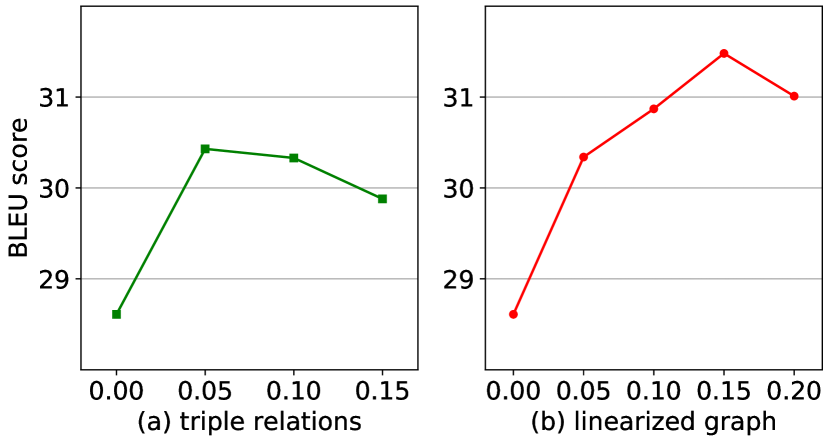
Figure 3: Development results on LDC2015E86.

For our approach, the multi-layer perceptrons for deep biaffine classifiers (Equations 6, 7, 9 and 10) take two layers of 512 units. The Transformer decoder (Equation 14) for predicting linearized graphs takes the same embedding and hidden sizes as the baseline decoder (Equation 4).

5.3 Development Results

Figure 3 shows the devset performances of using either Loss 1 (triple relations) or Loss 2 (linearized graph) under different coefficients. It shows the baseline performance when a coefficient equals to 0. There are large improvements in terms of BLEU score when increasing the coefficient of either loss from 0. These results indicate the effectiveness of our autoencoding training framework. The performance of our model with either loss slightly goes down when further increasing the coefficient. One underlying reason is that an over-large coefficient will dilute the primary signal on language modeling, which is more relevant to the BLEU metric. Particularly, we observe the highest performances when $\alpha$ and $\beta$ are 0.05 and 0.15, respectively, and thus we set our coefficients using these values for the remaining experiments.

5.4 Main Results

Model	BLEU	Time
LSTM (Konstas et al., 2017)	22.00	–
GRN (Song et al., 2018)	23.28	–
DCGCN (Guo et al., 2019)	25.70	–
RA-Trans-SA (Zhu et al., 2019)	29.66	–
RA-Trans-F-ours	29.11	0.25
+ Loss 1 (triple relations)	30.47	0.38
+ Loss 2 (linearized graph)	31.13	0.52
+ Both	31.41	0.61
DCGCN (0.3M)	33.2	–
GRN (2M)	33.6	–
LSTM (20M)	33.8	–
DCGCN (ensemble, 0.3M)	35.3	–

Table 1: Main test results on LDC2015E86. Numbers such as “2M” means the number of extra silver data being used, and “ensemble” indicates model ensemble.

Table 1 shows the main comparison results with existing work for AMR-to-text generation, where “Time” represents the average time (seconds) for training one step. The first group corresponds to the reported numbers of previous models on this dataset, and their main difference is the encoder for presenting graphs: LSTM (Konstas et al., 2017) applies a multi-layer LSTM on linearized AMRs, GRN (Song et al., 2018) and DCGCN (Guo et al., 2019) adopt graph neural networks to encode original AMRs, and RA-Trans-SA is the best performing model of Zhu et al. (2019), using self attention to model the relation path for each node pair.

The second group reports our systems, where the RA-Trans-F-ours baseline is our implementation of the feature-based model of Zhu et al. (2019). It shows a highly competitive performance on this dataset. Applying Loss 1 alone achieves an improvement of 1.36 BLEU points, and Loss 2 alone obtains 0.66 more points than Loss 1. One possible reason is that Loss 2, which aims to reconstruct the whole linearized graph, can provide more informative features. Using both losses, we observe roughly a 2.3-point gain in terms of BLEU, indicating that both losses are complementary.

Regarding Meteor, RA-Trans-SA reports 35.45, the highest among all previously reported numbers. The RA-Trans-F-ours baseline gets 35.0 that is slightly worse than RA-Trans-SA. Applying Loss 1 or Loss 2 alone gives a number of 35.5 and 36.1, respectively. Using both losses, our approach achieves 36.2 that is better than RA-Trans-SA.

Regarding the training speed, adopting Loss 2 requires double amount of time compared with the baseline, being much slower than Loss 1. This is because the biaffine attention calculations for different word pairs are parallelizable, while it is not for producing a linearized graph. Using both losses together, we observe a moderately longer training process (1.4-times slower) than the baseline. Please note that our autoencoding framework only affects the offline training procedure, leaving the online inference process unchanged.

The last group shows additional higher numbers produced by systems that use the ensemble of multiple models and/or additional silver data. They suffer from problems such as requiring massive computation resources and taking a long time for training. We leave exploring additional silver data and ensemble for further work.

5.5 Quantitative Human Study on Preserving Input Relation

Model	Recall (%)
RA-Trans-F-ours	78.00
+ Both	85.13

Table 2: Human study for the recall of input relations on LDC2015E86.

Our multi-view autoencoding framework aims at preserving input relations, thus we further conduct a quantitative human study to estimate this aspect. To this end, we first extract all interactions of a subject, a predict and an object (corresponding to the AMR fragment “pred :ARG0 subj :ARG1 obj”) from each AMR graph, and then check how many interactions are preserved by the output of a model. The reason for considering this type of interaction comes from two folds: first, they convey fundamental information forming the backbone of a sentence, and second, they can be easily extracted from graphs and evaluated by human judges.

As shown in Table 2, we choose 200 AMR-sentence pairs to conduct this study and compare our model with the baseline in terms of the recall number, showing the percent of preserved interactions. To determine if a sentence preserves an interaction, we ask 3 people with NLP background to make their decisions and choose the majority vote as the human judgement. Out of the 491 interactions, the baseline only preserves 78%. With our multi-view autoencoding losses, 7.13% more interactions are preserved, which further confirms the effectiveness of our approach.

5.6 Case Study

As shown in Table 3, we further demonstrate several typical examples from our human study for better understanding how our framework helps preserve structural input information. Each example includes an input AMR, a reference sentence (Ref), the baseline output (Baseline) and the generated sentence by our approach (Our approach).

(r / recommend-01

:ARG0 (i / i)

:ARG1 (g / go-02

:ARG0 (y / you)

:purpose (s / see-01

:ARG0 y

:ARG1 (p / person

:ARG0-of (h / have-rel-role-91

:ARG1 y

:ARG2 (d / doctor)))

:mod (t / too)))

:ARG2 y)

Ref: i ’d recommend you go and see your doctor too .

Baseline: i should go to see your doctor too .

Our approach: i recommend you to go to see your doctor too .

(c / country

:mod (o / only)

:ARG0-of (h / have-03

:ARG1 (p / policy

:consist-of (t / target-01

:ARG1 (a / aircraft

:ARG0-of (t2 / traffic-01

:ARG1 (d / drug)))))

:time (c3 / current))

:domain (c2 / country

:wiki “Colombia”

:name (n / name :op1 “Colombia”)))

Ref: colombia is the only country that currently has a policy of targeting drug trafficking aircraft .

Baseline: colombia is the only country with drug trafficking policy .

Our approach: colombia is the only country with the current policy of targets for drug trafficking aircraft .

Table 3: Example system outputs.

For the first example, the baseline output drops the key predicate “recommend” and fails to preserve the fact that “you” is the subject of “go”. The reason can be that “I should go to” occurs frequently in the training corpus. On the other hand, the extra signals produced by our multi-view framework enhance the input semantic information, guiding our model to generate a correct sentence with the exact meaning of the input AMR.

The second example shows a similar situation, where the baseline generates a natural yet short sentence that drops some important information from the input graph. As a result of the information loss, the resulting sentence conveys an opposite meaning (“with drug trafficking policy”) to the input (“targeting drug trafficking aircraft”). This is a typical problem suffered by many neural graph-to-sequence models. Our multi-view framework helps recover the correct meaning: “policy of target for drug trafficking aircraft”.

5.7 Ablation Study

Model	BLEU
RA-Trans-F-ours + Loss 1	30.47
w/o edge label	29.39
RA-Trans-F-ours + Loss 2	31.13
w/o edge label	30.36
random linearization	31.07

Table 4: Ablation study for both views.

As shown in Table 4, we conduct an ablation study on LDC2015E86 to analyze how important each part of the input graphs is under our framework. For Loss 1, we test the situation when no edge labels are available, and as a result, we observe a large performance drop of 1.0+ BLEU points. This is quite intuitive, because edge labels carry important relational knowledge between the two connected nodes. Therefore, discarding these labels will cause loss of significant semantic information.

For Loss 2, we also observe a large performance decrease when edge labels are dropped, confirming the observation for Loss 1. In addition, we study the effect of random graph linearization, where the order for picking children is random rather than following the left-to-right order at each stage of the depth-first traversal procedure. The motivation is to investigate the robustness of Loss 2 regarding input variances, as an organized input order (such as an alphabetical order for children) may not be available for certain graph-to-sequence tasks. We observe a marginal performance drop of less than 0.1 BLEU points, indicating that our approach is very robust for input variances. It is likely because different linearization results still indicate the same graph. Besides, one previous study (Konstas et al., 2017) shows a very similar observation.

5.8 Main Results on LDC2017T10

Model	BLEU	Meteor
DCGCN	27.60	–
RA-Trans-CNN	31.82	36.38
GPT-2L	32.47	36.80
GPT-2L re-scoring	33.02	37.68
RA-Trans-F-ours	31.77	37.2
+ Loss 1	33.98	37.5
+ Loss 2	34.13	37.8
+ Both	34.21	38.0

Table 5: Main test results on LDC2017T10.

Table 5 compares our results on LDC2017T10 with the highest numbers reported by single models without extra silver training data. GPT-2L Mager et al. (2020) applies a GPT-2 Large model Radford et al. (2019) on linearized AMR graphs, and GPT-2L re-scoring further performs re-scoring based on AMR back-parsing for post processing. RA-Trans-CNN is another model by Zhu et al. (2019) that adopt a convolutional neural network LeCun et al. (1990) to model the relation path for each node pair. Again, the RA-Trans-F baseline achieves a comparable score with RA-Trans-CNN, and our approach improves the baseline by nearly 2.5 BLEU points, indicating its superiority.

Regarding Meteor score, our advantage (1.62 points) over the previous state-of-the-art system on this dataset is larger than that (0.75 points) on LDC2015E86. Since LDC2017T10 has almost one time more training instances than LDC2015E86, we may conclude that the problem of dropping input information may not be effectively reduced by simply adding more supervised data, and as a result, our approach can still be effective on a larger dataset. This conclusion can also be confirmed by comparing the gains of our approach on both AMR datasets regarding BLEU score (2.3 vs 2.5).

5.9 Main Results on WebNLG

Table 6 shows the comparison of our results with previous results on the WebNLG testset. ADAPT (Gardent et al., 2017) is based on the standard encoder-decoder architecture (Cho et al., 2014) with byte pair encoding (Sennrich et al., 2016), and it was the best system of the challenge. GCN_EC (Marcheggiani and Perez-Beltrachini, 2018) is a recent model using a graph convolution network (Kipf and Welling, 2017) for encoding KGs.

Our baseline shows a comparable performance with the previous state of the art. Based on this baseline, applying either loss leads to a significant improvement, and their combination brings a gain of more than 2 BLEU points. Although the baseline already achieves a very high BLEU score, yet the gains on this task are still comparable with those on AMR-to-text generation. This observation may imply that the problem of missing input structural knowledge can be ubiquitous among many graph-to-text problems, and as a result, our approach can be widely helpful across many tasks.

Model	BLEU	Meteor
ADAPT	60.59	44.0
GCNEC	55.90	39.0
RA-Trans-F-ours	60.51	42.2
+ Loss 1	61.78	43.6
+ Loss 2	62.29	43.5
+ Both	62.89	44.2

Table 6: Main test results on WebNLG

Following previous work, we also report Meteor scores, where our approach shows a gain of 2 points against the baseline and our final number is comparable with ADAPT. Similar with the gains on the BLEU metric, Loss 1 is comparable with Loss 2 regarding Meteor, and their combination is more useful than applying each own.

6 Conclusion

We proposed reconstructing input graphs as autoencoding processes to encourage preserving the input semantic information for graph-to-text generation. In particular, the auxiliary losses for recovering two complementary views (triple relations and linearized graph) of input graphs are introduced, so that our model is trained to retain input structures for better generation. Our training framework is general for different graph types. Experiments on two benchmarks showed the effectiveness of our framework under both the automatic BLEU metric and human judgements.

References

- Aharoni and Goldberg (2017) Roee Aharoni and Yoav Goldberg. 2017. Towards string-to-tree neural machine translation. In Proceedings of the 55th Annual Meeting of the Association for Computational Linguistics (Volume 2: Short Papers).
- Balakrishnan et al. (2019) Anusha Balakrishnan, Jinfeng Rao, Kartikeya Upasani, Michael White, and Rajen Subba. 2019. Constrained decoding for neural NLG from compositional representations in task-oriented dialogue. In Proceedings of the 57th Annual Meeting of the Association for Computational Linguistics.
- Banarescu et al. (2013) Laura Banarescu, Claire Bonial, Shu Cai, Madalina Georgescu, Kira Griffitt, Ulf Hermjakob, Kevin Knight, Philipp Koehn, Martha Palmer, and Nathan Schneider. 2013. Abstract meaning representation for sembanking. In Proceedings of the 7th Linguistic Annotation Workshop and Interoperability with Discourse.
- Beck et al. (2018) Daniel Beck, Gholamreza Haffari, and Trevor Cohn. 2018. Graph-to-sequence learning using gated graph neural networks. In Proceedings of the 56th Annual Meeting of the Association for Computational Linguistics (Volume 1: Long Papers).
- Cai and Lam (2019) Deng Cai and Wai Lam. 2019. Graph transformer for graph-to-sequence learning. In Thirty-Fourth AAAI Conference on Artificial Intelligence.
- Cao and Clark (2019) Kris Cao and Stephen Clark. 2019. Factorising amr generation through syntax. In Proceedings of the 2019 Conference of the North American Chapter of the Association for Computational Linguistics: Human Language Technologies, Volume 1 (Long and Short Papers).
- Cho et al. (2014) Kyunghyun Cho, Bart van Merrienboer, Caglar Gulcehre, Dzmitry Bahdanau, Fethi Bougares, Holger Schwenk, and Yoshua Bengio. 2014. Learning phrase representations using rnn encoder–decoder for statistical machine translation. In Proceedings of the 2014 Conference on Empirical Methods in Natural Language Processing (EMNLP).
- Damonte and Cohen (2019) Marco Damonte and Shay B Cohen. 2019. Structural neural encoders for amr-to-text generation. In Proceedings of the 2019 Conference of the North American Chapter of the Association for Computational Linguistics: Human Language Technologies, Volume 1 (Long and Short Papers).
- Denkowski and Lavie (2014) Michael Denkowski and Alon Lavie. 2014. Meteor universal: Language specific translation evaluation for any target language. In Proceedings of the EACL 2014 Workshop on Statistical Machine Translation.
- Dozat and Manning (2017) Timothy Dozat and Christopher D Manning. 2017. Deep biaffine attention for neural dependency parsing. In International Conference on Learning Representations.
- Dušek et al. (2019) Ondřej Dušek, David M Howcroft, and Verena Rieser. 2019. Semantic noise matters for neural natural language generation. In Proceedings of the 12th International Conference on Natural Language Generation.
- Dušek et al. (2018) Ondřej Dušek, Jekaterina Novikova, and Verena Rieser. 2018. Findings of the e2e nlg challenge. In Proceedings of the 11th International Conference on Natural Language Generation.
- Flanigan et al. (2016) Jeffrey Flanigan, Chris Dyer, Noah A Smith, and Jaime Carbonell. 2016. Cmu at semeval-2016 task 8: Graph-based amr parsing with infinite ramp loss. In Proceedings of the 10th International Workshop on Semantic Evaluation (SemEval-2016).
- Gardent et al. (2017) Claire Gardent, Anastasia Shimorina, Shashi Narayan, and Laura Perez-Beltrachini. 2017. The webnlg challenge: Generating text from rdf data. In Proceedings of the 10th International Conference on Natural Language Generation.
- Guo et al. (2019) Zhijiang Guo, Yan Zhang, Zhiyang Teng, and Wei Lu. 2019. Densely connected graph convolutional networks for graph-to-sequence learning. Transactions of the Association for Computational Linguistics, 7.
- Hajdik et al. (2019) Valerie Hajdik, Jan Buys, Michael Wayne Goodman, and Emily M Bender. 2019. Neural text generation from rich semantic representations. In Proceedings of the 2019 Conference of the North American Chapter of the Association for Computational Linguistics: Human Language Technologies, Volume 1 (Long and Short Papers).
- Hochreiter and Schmidhuber (1997) Sepp Hochreiter and Jürgen Schmidhuber. 1997. Long short-term memory. Neural computation, 9(8).
- Hong et al. (2019) Xudong Hong, Ernie Chang, and Vera Demberg. 2019. Improving language generation from feature-rich tree-structured data with relational graph convolutional encoders. In Proceedings of the 2nd Workshop on Multilingual Surface Realisation (MSR 2019), pages 75–80.
- Iyer et al. (2017) Srinivasan Iyer, Ioannis Konstas, Alvin Cheung, Jayant Krishnamurthy, and Luke Zettlemoyer. 2017. Learning a neural semantic parser from user feedback. In Proceedings of the 55th Annual Meeting of the Association for Computational Linguistics (Volume 1: Long Papers), pages 963–973.
- Jia et al. (2019) Chen Jia, Xiaobo Liang, and Yue Zhang. 2019. Cross-domain ner using cross-domain language modeling. In Proceedings of the 57th Annual Meeting of the Association for Computational Linguistics.
- Kingma and Ba (2014) Diederik P Kingma and Jimmy Ba. 2014. Adam: A method for stochastic optimization. arXiv preprint arXiv:1412.6980.
- Kipf and Welling (2017) Thomas N Kipf and Max Welling. 2017. Semi-supervised classification with graph convolutional networks. In International Conference on Learning Representations.
- Koncel-Kedziorski et al. (2019) Rik Koncel-Kedziorski, Dhanush Bekal, Yi Luan, Mirella Lapata, and Hannaneh Hajishirzi. 2019. Text generation from knowledge graphs with graph transformers. In Proceedings of the 2019 Conference of the North American Chapter of the Association for Computational Linguistics: Human Language Technologies, Volume 1 (Long and Short Papers).
- Konstas et al. (2017) Ioannis Konstas, Srinivasan Iyer, Mark Yatskar, Yejin Choi, and Luke Zettlemoyer. 2017. Neural amr: Sequence-to-sequence models for parsing and generation. In Proceedings of the 55th Annual Meeting of the Association for Computational Linguistics (Volume 1: Long Papers).
- LeCun et al. (1990) Yann LeCun, Bernhard E Boser, John S Denker, Donnie Henderson, Richard E Howard, Wayne E Hubbard, and Lawrence D Jackel. 1990. Handwritten digit recognition with a back-propagation network. In Advances in neural information processing systems, pages 396–404.
- Li et al. (2016) Yujia Li, Daniel Tarlow, Marc Brockschmidt, and Richard Zemel. 2016. Gated graph sequence neural networks. In International Conference on Learning Representations.
- Liu et al. (2018a) Liyuan Liu, Jingbo Shang, Xiang Ren, Fangzheng Xu, Huan Gui, Jian Peng, and Jiawei Han. 2018a. Empower sequence labeling with task-aware neural language model. In Thirty-Second AAAI Conference on Artificial Intelligence.
- Liu et al. (2018b) Lizhen Liu, Xiao Hu, Wei Song, Ruiji Fu, Ting Liu, and Guoping Hu. 2018b. Neural multitask learning for simile recognition. In Proceedings of the 2018 Conference on Empirical Methods in Natural Language Processing.
- Liu et al. (2018c) Yijia Liu, Wanxiang Che, Bo Zheng, Bing Qin, and Ting Liu. 2018c. An amr aligner tuned by transition-based parser. In Proceedings of the 2018 Conference on Empirical Methods in Natural Language Processing.
- Mager et al. (2020) Manuel Mager, Ramón Fernandez Astudillo, Tahira Naseem, Md Arafat Sultan, Young-Suk Lee, Radu Florian, and Salim Roukos. 2020. GPT-too: A language-model-first approach for AMR-to-text generation. In Proceedings of the 58th Annual Meeting of the Association for Computational Linguistics.
- Marcheggiani and Perez-Beltrachini (2018) Diego Marcheggiani and Laura Perez-Beltrachini. 2018. Deep graph convolutional encoders for structured data to text generation. In Proceedings of the 11th International Conference on Natural Language Generation.
- Nivre (2003) Joakim Nivre. 2003. An efficient algorithm for projective dependency parsing. In Proceedings of the Eighth International Conference on Parsing Technologies.
- Papineni et al. (2002) Kishore Papineni, Salim Roukos, Todd Ward, and Wei-Jing Zhu. 2002. Bleu: a method for automatic evaluation of machine translation. In Proceedings of the 40th annual meeting on association for computational linguistics.
- Pourdamghani et al. (2014) Nima Pourdamghani, Yang Gao, Ulf Hermjakob, and Kevin Knight. 2014. Aligning english strings with abstract meaning representation graphs. In Proceedings of the 2014 Conference on Empirical Methods in Natural Language Processing (EMNLP).
- Radford et al. (2019) Alec Radford, Jeffrey Wu, Rewon Child, David Luan, Dario Amodei, and Ilya Sutskever. 2019. Language models are unsupervised multitask learners. OpenAI Blog, 1(8):9.
- Rei (2017) Marek Rei. 2017. Semi-supervised multitask learning for sequence labeling. In Proceedings of the 55th Annual Meeting of the Association for Computational Linguistics (Volume 1: Long Papers).
- Rei and Søgaard (2019) Marek Rei and Anders Søgaard. 2019. Jointly learning to label sentences and tokens. In Proceedings of the AAAI Conference on Artificial Intelligence.
- Ribeiro et al. (2019) Leonardo FR Ribeiro, Claire Gardent, and Iryna Gurevych. 2019. Enhancing amr-to-text generation with dual graph representations. In Proceedings of EMNLP-IJCNLP.
- Sennrich et al. (2016) Rico Sennrich, Barry Haddow, and Alexandra Birch. 2016. Neural machine translation of rare words with subword units. In Proceedings of the 54th Annual Meeting of the Association for Computational Linguistics (Volume 1: Long Papers).
- Song et al. (2019) Linfeng Song, Daniel Gildea, Yue Zhang, Zhiguo Wang, and Jinsong Su. 2019. Semantic neural machine translation using amr. Transactions of the Association for Computational Linguistics, 7:19–31.
- Song et al. (2018) Linfeng Song, Yue Zhang, Zhiguo Wang, and Daniel Gildea. 2018. A graph-to-sequence model for amr-to-text generation. In Proceedings of the 56th Annual Meeting of the Association for Computational Linguistics (Volume 1: Long Papers).
- Su et al. (2017) Jinsong Su, Zhixing Tan, Deyi Xiong, Rongrong Ji, Xiaodong Shi, and Yang Liu. 2017. Lattice-based recurrent neural network encoders for neural machine translation. In Thirty-First AAAI Conference on Artificial Intelligence.
- Szubert et al. (2018) Ida Szubert, Adam Lopez, and Nathan Schneider. 2018. A structured syntax-semantics interface for english-amr alignment. In Proceedings of the 2018 Conference of the North American Chapter of the Association for Computational Linguistics: Human Language Technologies, Volume 1 (Long Papers).
- Trisedya et al. (2018) Bayu Distiawan Trisedya, Jianzhong Qi, Rui Zhang, and Wei Wang. 2018. Gtr-lstm: A triple encoder for sentence generation from rdf data. In Proceedings of the 56th Annual Meeting of the Association for Computational Linguistics (Volume 1: Long Papers), volume 1.
- Tu et al. (2017) Zhaopeng Tu, Yang Liu, Lifeng Shang, Xiaohua Liu, and Hang Li. 2017. Neural machine translation with reconstruction. In Thirty-First AAAI Conference on Artificial Intelligence.
- Vaswani et al. (2017) Ashish Vaswani, Noam Shazeer, Niki Parmar, Jakob Uszkoreit, Llion Jones, Aidan N Gomez, Łukasz Kaiser, and Illia Polosukhin. 2017. Attention is all you need. In Advances in neural information processing systems.
- Veličković et al. (2018) Petar Veličković, Guillem Cucurull, Arantxa Casanova, Adriana Romero, Pietro Lio, and Yoshua Bengio. 2018. Graph attention networks. In International Conference on Learning Representations.
- Wang and Xue (2017) Chuan Wang and Nianwen Xue. 2017. Getting the most out of amr parsing. In Proceedings of the 2017 conference on empirical methods in natural language processing.
- Wang et al. (2020) Tianming Wang, Xiaojun Wan, and Hanqi Jin. 2020. Amr-to-text generation with graph transformer. Transactions of the Association for Computational Linguistics, 8:19–33.
- Wang et al. (2018) Xinyi Wang, Hieu Pham, Pengcheng Yin, and Graham Neubig. 2018. A tree-based decoder for neural machine translation. In Proceedings of the 2018 Conference on Empirical Methods in Natural Language Processing.
- Wiseman et al. (2017) Sam Wiseman, Stuart M Shieber, and Alexander M Rush. 2017. Challenges in data-to-document generation. In Proceedings of the 2017 Conference on Empirical Methods in Natural Language Processing, pages 2253–2263.
- Wu et al. (2017) Shuangzhi Wu, Dongdong Zhang, Nan Yang, Mu Li, and Ming Zhou. 2017. Sequence-to-dependency neural machine translation. In Proceedings of the 55th Annual Meeting of the Association for Computational Linguistics (Volume 1: Long Papers).
- Xu et al. (2018) Kun Xu, Lingfei Wu, Zhiguo Wang, Yansong Feng, and Vadim Sheinin. 2018. Sql-to-text generation with graph-to-sequence model. In Proceedings of the 2018 Conference on Empirical Methods in Natural Language Processing, pages 931–936.
- Zhu et al. (2019) Jie Zhu, Junhui Li, Muhua Zhu, Longhua Qian, Min Zhang, and Guodong Zhou. 2019. Modeling graph structure in transformer for better amr-to-text generation. In Proceedings of EMNLP-IJCNLP.