Appearance of random matrix theory in deep learning

Abstract

We investigate the local spectral statistics of the loss surface Hessians of artificial neural networks, where we discover agreement with Gaussian Orthogonal Ensemble statistics across several network architectures and datasets. These results shed new light on the applicability of Random Matrix Theory to modelling neural networks and suggest a role for it in the study of loss surfaces in deep learning.

[bris]organization=School of Mathematics, University of Bristol,addressline=Fry Building, Woodland Road, city=Bristol, postcode=BS8 1UG, country=United Kingdom

[oxml]organization=Machine Learning Research Group, University of Oxford,addressline=Walton Well Road, city=Oxford, postcode=OX2 6ED, , country=United Kingdom

[oxmi]organization=Mathematical Institute, University of Oxford,addressline=Andrew Wiles Building, Woodstock Road, city=Oxford, postcode=OX2 6GG, , country=United Kingdom

1 Introduction

Artificial Neural Networks (ANNs) continually advance the state of the art in machine learning, including computer vision, speech processing and natural language processing. However, we do not have a precise theoretical understanding of their training and generalisation dynamics. The observation that gradient based optimisation methods [17] with different random initialisations do not seem to get stuck in poor quality local minima, despite the high dimensionality and non-convexity of the optimisation problems, has led to a significant focus on neural network loss surfaces.

The loss of a neural network is a scalar function that measures how well the network is performing on a particular data item, with lower values being better. Loss functions are defined to be greater than or equal to zero. For example, a neural network’s output may be the predicted house price given a set of features about the house, and the loss value for a particular house could be the squared error of the predicted price compared to the known true price. The loss surface of a neural network is the value of the loss, averaged over the data (houses in the above example) and viewed as a function of the network weights, i.e. its free parameters. The task of optimisation for neural networks amounts to finding low-points of the loss surface in a weight space which is typically very high dimensional (e.g. $10^{7}$ is not uncommon in practice). The loss surface in most realistic examples will be non-convex and possess many local minima and saddle points (though one notable exception is the common practice of training only the final layer of a deep network). The loss is almost always optimised using stochastic gradient descent (or some variant thereof such as Adam [46] or Adagrad [27], which use a per-parameter learning rate which depends on the running covariance of the gradients) and so one expects the local minima and low index saddle points to be important, being the points where the optimisation is likely to become trapped.

The loss surface is typically investigated through the Hessian which is the second order taylor expansion of the loss and hence especially relevant at local minima. Under strong simplifying assumptions, such as independence of the neural network inputs and weights [22, 23, 63], the Hessian at critical points of the loss (where the gradient is zero), is described by certain important classes of random matrices, such as the Gaussian Orthogonal Ensemble (GOE) [76] or the Wishart Ensemble [18] of Random Matrix Theory (RMT). The average spectral density (taken over an ensemble) of these matrices, in the limit of infinite dimension, can be calculated; for the GOE the result is known as the Wigner semicircle law, and for the Wishart Ensemble it is the Marchenko-Pastur law. Hence with these assumptions, one can make quantitative predictions about the nature of the critical points and aspects of the geometry of the loss landscape.

Several authors have studied the similarity between types of neural networks and models from statistical physics, such as spin glasses starting with Amit et al. [4], Gardner and Derrida [34], and more recently connections with the ANNs of machine learning, both empirical [69] and theoretical [22]. Chaudhari and Soatto [21] introduce connections with magnetic fields in disordered systems, demonstrating an analogy with weight decay in DNNs. Connections between machine learning and statistical physics from various viewpoints are detailed extensively in [8, 58, 79, 20, 33, 67].

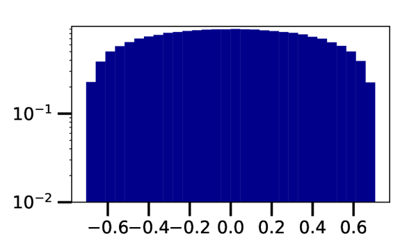
(a) Wigner semicircle

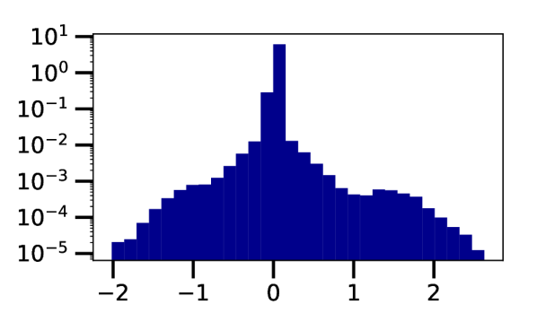
(b) MLP

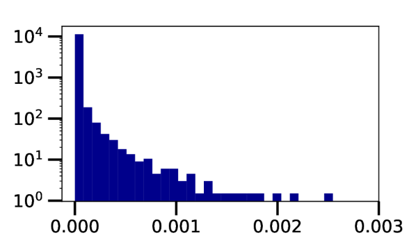
(c) Logistic Regression

Figure 1: Comparison of different global spectral statistics (spectral densities). (a) We show actual GOE data to demonstrate the form of the Wigner semicircle. (b) Hessian of cross entropy loss for MLP on MNIST. (c) Hessian of cross entropy loss for logistic regression on MNIST. Note the log-scale on the y-axis. A few outliers have been clipped from logistic regression to aid visualisation.

Choromanska et al. [22] showed, assuming i.i.d Gaussian inputs and network path independence, that a multi-layer ReLU neural network’s loss is equivalent to that of a spin-glass model. Its conditional Hessian spectrum is thus given by a GOE calculation [6] involving real-symmetric matrices with otherwise independent Gaussian random entries. It follows that under these assumptions local minima are located within a narrow band, bounded below by the global minimum. The practical implication is that for a sufficient number of hidden layers (more than 2) all local minima are close in loss to the global minimum. Baskerville et al. [9] extend this line of work to networks with general activation functions. Baskerville et al. [10] show for Generative Adversarial Networks, using a spin-glass model for both the generator and discriminator, that the structure of local optima encourages collapse to a narrow band of the loss for at least one of the networks but not necessarily both simultaneously. These works are examples of complexity calculations, which have a considerable history in the physics and mathematics literature [29, 32, 30]. Recent works have completed complexity calculations and studied properties of local minima of various models intended to highlight aspects of loss surfaces in high dimensions [68, 72, 51, 31]. Similarly, Pennington and Bahri [63] use the Gauss Newton decomposition of a squared loss Hessian, assuming independence and normality of both the data and weights along with free addition of the resulting Wigner/Wishart ensembles, to derive a functional form for the critical index (the fraction of the eigenvalues that are negative) as a function of the loss. They show that below a certain critical energy threshold all critical points are minima.

Several works have used randomised models of neural networks to study properties of the training and test loss, such as the double-descent phenomenon. The phenomenon can be recovered using randomised models of neural networks, such as random feature models (two-layer networks training only the last layer where the output of the first layer is i.i.d. Gaussian) [56, 35, 26]. Ba et al. [7] extended this analysis to two layer networks where either of the layers can be trained and demonstrated that the double-descent cannot be recovered when training only the lower layer. Combined with the work of Adlam and Pennington [2], the emerging understanding is that important properties of neural networks observed in practice can be recreated using simplified randomised models and random matrix theory, but the picture is far from complete.

Pennington and Worah have studied Gram matrices of network outputs [65] and also neural network Fisher information matrices [64] in the context of single hidden layer networks with i.i.d. Gaussian weights and inputs. Benigni and Péché [12] extended this work to any number of layers and i.i.d. weights and inputs with sub-Gaussian tails.

An important and fundamental problem with the aforementioned works is that typically the average spectral density of the Hessian of neural networks does not in fact match that of the associated random matrix ensembles. This is illustrated in Figure 1. Put simply, one does not observe the Wigner semicircle or Marchenko-Pastur eigenvalue distributions, implied by the Gaussian Orthogonal or Wishart Ensembles for ANNs. As shown in Granziol [38], Granziol et al. [39], Papyan [59, 60], Ghorbani et al. [36], Sagun et al. [70, 71] the spectral density of ANN Hessians contain outliers and a large number of near zero eigenvalues, features not seen in canonical random matrix ensembles. Furthermore, even allowing for this, as shown in [41] by specifically embedding outliers as a low rank perturbation to a random matrix, the remaining bulk spectral density still does not match the Wigner semicircle or Marchenko-Pastur distributions [38], bringing into question the validity of the underlying modelling.

The fact that the experimental results differ markedly from the theoretical predictions has called into question the validity of ANN analyses based on canonical random matrix ensembles. Moreover, the compelling results of works such as [22, 63] are obtained using very particular properties of the canonical ensembles, such as large deviation principles, as pointed out in Granziol [38]. The extent to which such results can be generalised is an open question. Hence, further work is required to better understand to what extent Random Matrix Theory can be used to analyse the loss surfaces of ANNs.

In the present paper, we show that the local spectral statistics (i.e. those measuring correlations on the scale of the mean eigenvalue spacing) of ANN Hessians are well modelled by those of GOE random matrices, even when the mean spectral density is different from the semicicle law. We display these results experimentally on MNIST trained multi-layer perceptrons and on the final layer of a ResNet-$34$ on CIFAR-$10$. The objective of our work is to motivate a new use for Random Matrix Theory in the study of the theory of deep neural networks.. In the context of more established applications of Random Matrix Theory, this conclusion may not be so surprising – it has often been observed that the local spectral statistics are universal while the mean density is not – however, in the context of Machine Learning this important point has not previously been made, nor its consequences explored. Our main goal is to illustrate it in that setting, through numerical experiments, and to start to examine some of its implications.

2 Preliminaries

Consider a neural network with weights $\bm{w}\in\mathbb{R}^{P}$ and a dataset with distribution $\mathbb{P}_{\mathrm{data}}$. For the purposes of our discussion, a neural network, $f_{\bm{w}}$ say, is just a non-linear function from some $\mathbb{R}^{d}$ to some $\mathbb{R}^{c}$, parametrised by $\bm{w}$. Neural networks can be defined in many different ways in terms of their weights (the architecture of the network), but these details will not play role in our discussion. What will be important is that the number of weights $P$ will be large, i.e. approaching 10,000 even in the simplest of cases. Let $L(\bm{w},\bm{x})$ be the loss of the network for a single datum $\bm{x}$ and let $\mathcal{D}$ denote any finite sample of data points from $\mathbb{P}_{\mathrm{data}}$. A simple example of $L$ is the squared error $L(\bm{w},(\bm{x},\bm{y}))=||f_{\bm{w}}(\bm{x})-\bm{y}||_{2}^{2}$, where $\mathbb{P}_{\mathrm{data}}$ is a distribution on tuples of features $\bm{x}$ and labels $\bm{y}$. The true loss is given by

$$\mathcal{L}_{true}(\bm{w})=\mathbb{E}_{\bm{x}\sim\mathbb{P}_{\mathrm{data}}}L(\bm{w},\bm{x})$$ (1)

and the empirical loss (or training loss) is given by

$$\mathcal{L}_{emp}(\bm{w},\mathcal{D})=\frac{1}{|\mathcal{D}|}\sum_{\bm{x}\in\mathcal{D}}L(\bm{w},\bm{x}).$$ (2)

Where $\mathcal{D}$ denotes the dataset. The true loss is a deterministic function of the weights, while the empirical loss is a random function with the randomness coming from the random sampling of the finite dataset $\mathcal{D}$. The empirical Hessian ${\bm{H}}_{emp}({\bm{w}})=\nabla^{2}\mathcal{L}_{emp}({\bm{w}})$, describes the loss curvature at the point ${\bm{w}}$ in weight space. By the spectral theorem, the Hessian can be written in terms of its eigenvalue/eigenvector pairs ${\bm{H}}_{emp}=\sum_{i}^{P}\lambda_{i}{\bm{\phi}}_{i}{\bm{\phi}}_{i}^{T}$, where the dependence on ${\bm{w}}$ has been dropped to keep the notation simple. The eigenvalues of the Hessian are particularly important, being explicitly required in second-order optimisation methods, and characterising the stationary points of the loss as local minima, local maxima or generally saddle points of some other index.

For a matrix drawn from a probability distribution, its eigenvalues are random variables. The eigenvalue distribution is described by the joint probability density function (j.p.d.f) $p(\lambda_{1},\lambda_{2},\ldots,\lambda_{P})$, also known as the $P$-point correlation function. The simplest example is the empirical spectral density (ESD), $\rho^{(P)}(\lambda)=\frac{1}{P}\sum_{i}^{P}\delta(\lambda-\lambda_{i})$. Integrating $\rho^{(P)}(\lambda)$ over an interval with respect to $\lambda$ gives the fraction of the eigenvalues in that interval. Taking an expectation over the random matrix ensemble, we obtain the mean spectral density $\mathbb{E}\rho^{(P)}(\lambda)$, which is a deterministic probability distribution on $\mathbb{R}$. Alternatively, taking the $P\rightarrow\infty$ limit, assuming it exists, gives the limiting spectral density (LSD) $\rho$, another deterministic probability distribution on $\mathbb{R}$. A key feature of many random matrix ensembles is self-averaging or ergodicity, meaning that the leading order term (for large $P$) in $\mathbb{E}\rho^{(P)}$ agrees with $\rho$. Given the j.p.d.f, one can obtain the mean spectral density, known as the $1$-point correlation function (or any other $k$-point correlation function) by marginalisation

$$\mathbb{E}\rho^{(P)}(\lambda)=\int p(\lambda,\lambda_{2},\ldots,\lambda_{P})d\lambda_{2}\ldots d\lambda_{P}.$$ (3)

A GOE matrix is an example of a Wigner random matrix, namely a real-symmetric (or complex-Hermitian) matrix with otherwise i.i.d. entries and off-diagonal variance $\sigma^{2}$. The mean spectral density for Wigner matrices is known to be Wigner’s semicircle [55]

$$\rho_{SC}(\lambda)=\frac{1}{2\pi\sigma^{2}P}\sqrtsign{4P\sigma^{2}-\lambda^{2}}\mathbf{1}_{|\lambda|\leq 2\sigma\sqrtsign{P}}.$$ (4)

The radius of the semicircle is proportional to $\sqrtsign{P}\sigma$, hence scaling Wigner matrices by $1/\sqrt{P}$ leads to a limit distribution when $P\rightarrow\infty$. This is the LSD. With this scaling, there are, on average, $\mathcal{O}(P)$ eigenvalues in any open subset of the compact spectral support. In this sense, the mean (or limiting) spectral density is macroscopic, meaning that, as $P\rightarrow\infty$, one ceases to see individual eigenvalues, but rather a continuum with some given density.

3 Motivation: Microscopic Universality

Random Matrix Theory was first developed in physics to explain the statistical properties of nuclear energy levels, and later used to describe the spectral statistics in atomic spectra, condensed matter systems, quantum chaotic systems etc; see, for example [78, 11, 14, 16]. None of these physical systems exhibits a semicircular empirical spectral density. However they all generically show agreement with RMT at the level of the mean eigenvalue spacing when local spectral statistics are compared. Our point is that while neither multi-layer perceptron (MLP) nor Softmax Regression Hessians are described by the Wigner semicircle law which holds for GOE matrices (c.f. Figure 1a) – their spectra contain outliers, large peaks near the origin and the remaining components of the histogram also do not match the semicircle – nevertheless Random Matrix Theory can still (and we shall demonstrate does) describe spectral fluctuations on the scale of their mean eigenvalue spacing.

It is worth noting in passing that possibilities other than random-matrix statistics exist and occur. For example, in systems that are classically integrable, one finds instead Poisson statistics [15, 14]; similarly, Poisson statistics also occur in disordered systems in the regime of strong Anderson localisation [28]; and for systems close to integrable one finds a superposition of random-matrix and Poisson statistics [13]. So showing that Random Matrix Theory applies is far from being a trivial observation. Indeed it remains one of the outstanding challenges of mathematical physics to prove that the spectral statistics of any individual Hamiltonian system are described by it in the semiclassical limit.

Physics RMT calculations re-scale the eigenvalues to have a mean level spacing of $1$ and then typically look at the nearest neighbour spacings distribution (NNSD), i.e. the distribution of the distances between adjacent pairs of eigenvalues. One theoretical motivation for considering the NNSD is that it is independent of the Gaussianity assumption and reflects the symmetry of the underlying system. It is the NNSD that is universal (for systems of the same symmetry class) and not the average spectral density, which is best viewed as a parameter of the system. The aforementioned transformation to give mean spacing $1$ is done precisely to remove the effect of the average spectral density on the pair correlations leaving behind only the universal correlations. To the best of our knowledge no prior work has evaluated the NNSD of artificial neural networks and this is a central focus of this paper.

In contrast to the LSD, other $k$-point correlation functions are also normalised such that the mean spacing between adjacent eigenvalues is unity. At this microscopic scale, the LSD is locally constant and equal to 1 meaning that its effect on the eigenvalues’ distribution has been removed and only microscopic correlations remain. In the case of Wigner random matrices, for which the LSD varies slowly across the support of the eigenvalue distribution, this corresponds to scaling by $\sqrt{P}$. On this scale the limiting eigenvalue correlations when $P\to\infty$ are universal; that is, they are the same for wide classes of random matrices, depending only on symmetry [42]. For example, this universality is exhibited by the NNSD. Consider a $2\times 2$ GOE matrix, in which case the j.p.d.f has a simple form:

$$p(\lambda_{1},\lambda_{2})\propto|\lambda_{1}-\lambda_{2}|e^{-\frac{1}{2}(\lambda_{1}^{2}+\lambda_{2}^{2})}.$$ (5)

Making the change of variables $\nu_{1}=\lambda_{1}-\lambda_{2},\nu_{2}=\lambda_{1}+\lambda_{2}$, integrating out $\nu_{2}$ and setting $s=|\nu_{1}|$ results in a density $\rho_{Wigner}(s)=\frac{\pi s}{2}e^{-\frac{\pi}{4}s^{2}}$, known as the Wigner surmise (see Figure 2). For larger matrices, the j.p.d.f must include an indicator function $\mathbbm{1}\{\lambda_{1}\leq\lambda_{2}\leq\ldots\lambda_{P}\}$ before marginalisation so that one is studying pairs of adjacent eigenvalues. While the Wigner surmise can only be proved exactly, as above, for the 2 × 2 GOE, it holds to high accuracy for the NNSD of GOE matrices of any size provided that the eigenvalues have been scaled to give mean spacing 1. The Wigner surmise density vanishes at $0$, capturing ‘repulsion’ between eigenvalues that is characteristic of RMT statistics, in contrast to the distribution of entirely independent eigenvalues given by the Poisson law $\rho_{Poisson}(s)=e^{-s}$. The Wigner surmise is universal in that the same density formula applies to all real-symmetric random matrices, not just the GOE or Wigner random matrices.

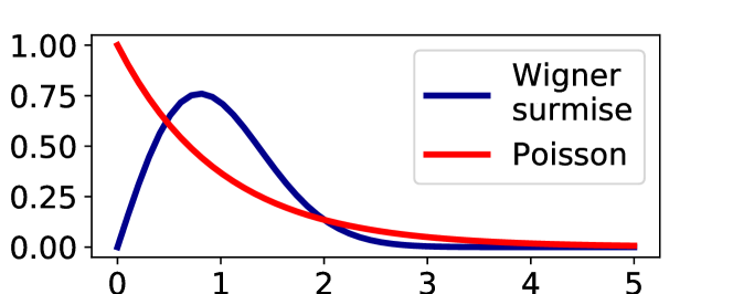
Figure 2: The density of the Wigner surmise.

4 Methodology

Prior work [40, 59, 36] focusing on the Hessian empirical spectral density has utilised fast Hessian vector products [62] in conjunction with Lanczos [57] methods. However, these methods approximate only macroscopic quantities like the spectral density, not microscopic statistics such as nearest neighbour spectral spacings. For modern neural networks, the $\mathcal{O}(P^{3})$ Hessian eigendecomposition cost will be prohibitive, e.g. for a Residual Network (Resnet) [44] with $34$ layers $P=10^{7}$. Hence, We restrict to models small enough to perform exact full Hessian computation and eigendecomposition.

We consider single layer neural networks for classification (softmax regression), 2-hidden-layer MLPs and 3 hidden-layer MLPs. On MNIST [25], the Hessians are of size $7850\times 7850$ for logistic regression, $9860\times 9860$ for the small MLP and $20060\times 20060$ for the larger 3 hidden-layer MLP, so can be computed exactly by simply applying automatic differentiation twice, and the eigenvalues can be computed exactly in a reasonable amount of time. We also consider a single layer applied to CIFAR-$10$ [47] classification with pre-trained Resnet-$34$ embedding features [44, 66]. While we cannot at present study the full Hessian of, for example, a Resnet-$34$, we can study the common transfer learning use-case of training only the final layer on some particular task [75]. The Hessians can be computed at any data point or over any collection of data points. We consider Hessians computed over the entire datasets in question, and over batches of size 64. We separately consider test and train sets.

In order to extend the relevance of our analysis to beyond logistic regression and MLP, we consider one of the simplest convolutional neural networks (CNN) of the form of LeNet [48] on CIFAR-$10$. Compared to the standard LeNet (which has over $50000$ parameters) we reduce the number of neurons in the first fully connected layer from $120$ to $35$ and the second from $84$ to $50$. Note that the resulting architecture contains a bottleneck in the intermediate layer, in contrast to the “hour-glass” shapes that are necessary to maintain manageable parameter numbers with full MLP architectures. Despite reducing the total number of parameters by a factor of $3$ we find the total validation accuracy drop to be no more than $2\%$. The total validation accuracy of $69\%$ is significantly below state of the art $\approx 95\%$, but we are clearly in the regime where significant learning can and does take place, which we consider sufficient for the purposes of this manuscript. We also extend our experiments beyond the cross entropy loss function, by considering a regression problem ($L_{2}$ loss) and beyond the high-dimensional feature setting of computer vision with the Bike dataset which has only 13-dimensional feature vectors and a single-dimensional regressand (see Appendix B.3 for details of our data pre-processing). The architecture in this case widens considerably in the first layer (from 13 inputs to 100 neurons) and that gradually tapers to the single output. The final test loss (i.e. mean squared error) of the trained model is 0.044 which is competitive with baseline results [77]

Training details:

All networks were trained using SGD for 300 epochs with initial learning rate 0.003, linear learning rate decay to 0.00003 between epoch 150 and 270, momentum 0.9 and weight decay $5\times 10^{-4}$. We use a PyTorch [61] implementation. Full code to reproduce our results is made available . Full descriptions of all network architectures are given in the Appendix B.

5 Spectral spacing statistics in RMT

Consider a random $P\times P$ matrix $M_{P}$ with ordered $\lambda_{1}\leq\lambda_{2}\leq\ldots\leq\lambda_{P}$. Let $I_{ave}$ be the mean spectral cumulative density function for the random matrix ensemble from which $M_{P}$ is drawn. The unfolded spectrum is defined as

$$l_{i}=I_{ave}(\lambda_{i}).$$ (6)

The unfolded spacings are then defined as

$$s_{i}=l_{i}-l_{i-1},~{}~{}~{}i=2,\ldots,P.$$ (7)

With this definition, the mean of the $s_{i}$ is unity, which means that this transformation has brought the eigenvalues on to the microscopic scale on which universal spectral spacing statistics emerge. We are investigating the presence of Random Matrix Theory statistics in neural networks by considering the nearest neighbour spectral spacings of their Hessians. Within the Random Matrix Theory literature, it has been repeatedly observed [16, 14] that the unfolded spacings of a matrix with RMT pair correlations follow universal distributions determined only by the symmetry class of the $M_{P}$. Hessians are real symmetric, so the relevant universality class is GOE and therefore the unfolded neural network spacings should be compared to the Wigner surmise

$$\rho_{Wigner}(s)=\frac{\pi s}{2}e^{-\frac{\pi}{4}s^{2}}.$$ (8)

A collection of unfolded spacings $s_{2},\ldots,s_{P}$ from a matrix with GOE spacing statistics should look like a sample of i.i.d. draws from the Wigner surmise density (8). For some known random matrix distributions, $I_{ave}$ may be available explicitly, or at least via highly accurate quadrature methods from a known mean spectral density. For example, for the $P\times P$ GOE [1] $I_{ave}^{GOE}(\lambda)$ is given by:

$$P\left[\frac{1}{2}+\frac{\lambda}{2\pi P}\sqrt{2P-\lambda^{2}}+\frac{1}{\pi}\arctan\left(\frac{\lambda}{\sqrt{2P-\lambda^{2}}}\right)\right].$$ (9)

However, when dealing with experimental data where the mean spectral density is unknown, one must resort to using an approximation to $I_{ave}$. Various approaches are used in the literature, including polynomial spline interpolation [1]. The approach of [74, 73] is most appropriate in our case, since computing Hessians over many mini-batches of data results in a large pool of spectra which can be used to accurately approximate $I_{ave}$ simply by the empirical cumulative density. Suppose that we have $m$ samples $(M^{(i)}_{P})_{i=1}^{m}$ from a random matrix distribution over symmetric $P\times P$ matrices. Fix some integers $m_{1},m_{2}>0$ such that $m_{1}+m_{2}=m$. The spectra of the matrices $(M^{(i)}_{P})_{i=1}^{m_{1}}$ can then be used to construct an approximation to $I_{ave}$. More precisely, let $\Lambda_{1}$ be the set of all eigenvalues of the $(M^{(i)}_{P})_{i=1}^{m_{1}}$, then we define

$$\tilde{I}_{ave}(\lambda)=\frac{1}{|\Lambda_{1}|}|\{\lambda^{\prime}\in\Lambda_{1}\mid\lambda^{\prime}<\lambda\}|.$$ (10)

For each of the matrices $(M^{(i)}_{P})_{i=m_{1}+1}^{m}$, one can then use $\tilde{I}_{ave}$ to construct their unfolded spacings. When the matrix size $P$ is small, one can only study the spectral spacing distribution by looking over multiple matrix samples. However, the same spacing distribution is also present for a single matrix in the large $P$ limit. A clear disadvantage of studying unfolded nearest neighbour spectral spacings with the above methods is the need for a reasonably large number of independent matrix samples. This rules-out studying the unfolded spacings of a single large matrix. Another obvious disadvantage is the introduction of error by the approximation of $I_{ave}$, giving the opportunity for local spectral statistics to be distorted or destroyed. An alternative statistic is the consecutive spacing ratio of [5]. In the above notation, the ratios for a single $P\times P$ matrix are defined as

$$r_{i}=\frac{\lambda_{i}-\lambda_{i-1}}{\lambda_{i-1}-\lambda_{i-2}},~{}~{}2\leq i\leq P.$$ (11)

Atas et al. [5] proved a ‘Wigner-like surmise’ for the spacing ratios, which for the GOE is

$$P(r)=\frac{27(r+r^{2})}{8(1+r+r^{2})^{5/2}}.$$ (12)

In our experiments, we can compute the spacing ratios for Hessians computed over entire datasets or over batches, whereas the unfolded spacing ratios can only be computed in the batch setting, in which case a random $\frac{2}{3}$ of the batch Hessians are reserved for computing $\tilde{I}_{ave}$ and the remaining $\frac{1}{3}$ are unfolded and analysed. This split is essentially arbitrary, except that we err on the side of using more to compute $\tilde{I}_{ave}$ since even a single properly unfolded spectrum can demonstrate universal local statistics.

6 Results

We display results as histograms of data along with a plot of the Wigner (or the Wigner-like) surmise density. We make a few practical adjustments to the plots. Spacing ratios are truncated above some value, as the presence of a few extreme outliers makes visualisation difficult. We choose a cut-off at 10. Note that around 0.985 of the mass of the Wigner-like surmise is below 10, so this is a reasonable adjustment. The hessians have degenerate spectra. The Wigner surmise is not a good fit to the observed unfolded spectra if the zero eigenvalues are retained. Imposing a lower cut-off of $10^{-20}$ in magnitude is sufficient to obtain agreement with Wigner. This is below the machine precision, so these omitted eigenvalues are indistinguishable from 0.

(a)

(b)

Figure 3: Spacing distributions for the Hessian of a logistic regression trained Resnet-$34$ embeddings of CIFAR10. Hessians computed over the test set.

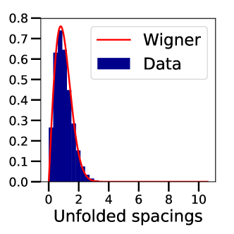
(a)

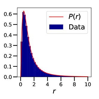
(b)

Figure 4: Spacing distributions for the Hessian of a 3-hidden-layer MLP trained on MNIST. Hessians computed over the test set.

6.1 MNIST and MLPs

We show results in Figures 3 and 4, with further plots in the supplementary material. We also considered randomly initialised networks and we evaluated the Hessians over train and test datasets separately in all cases. Unfolded spacings were computed only for Hessians evaluated on batches of 64 data points, while spacing ratios were computed in batches and over the entire dataset. We observe a striking level of agreement between the observed spectra and the GOE. There was no discernible difference between the train and test conditions, nor between batch and full dataset conditions, nor between trained and untrained models. Note that the presence of GOE statistics for the untrained models is not a foregone conclusion. Of course, the weights of the model are indeed random Gaussian, but the Hessian is still a function of the data set, so it is not the case the Hessian eigenvalue statistics are bound to be GOE a priori. Overall, the very close agreement between Random Matrix Theory predictions and our observations for several different architectures, model sizes and datasets demonstrates a clear presence of RMT statistics in neural networks.

Our results indicate that models for the loss surfaces of large neural networks should include assumptions of GOE local statistics of the Hessian, but ideally avoid such assumptions on the global statistics. To further illustrate this point, consider a Gaussian process $\mathcal{L}_{emp}\sim\mathcal{GP}(0,k)$ where $k$ is some kernel function. Following from our Gaussian process definition, the covariance of derivatives of the empirical loss can be computed using a well-known result (see Adler and Taylor [3] equation 5.5.4), e.g.

$$Cov(\partial_{i}\mathcal{L}_{emp}(\bm{w}),\partial_{j}\mathcal{L}_{emp}(\bm{w}^{\prime}))=\partial_{w_{i}}\partial_{w^{\prime}_{j}}k(\bm{w},\bm{w}^{\prime})$$

and further, assuming a stationary kernel $k(\bm{w},\bm{w}^{\prime})=k\left(-\frac{1}{2}||\bm{w}-\bm{w}^{\prime}||_{2}^{2}\right)$ (note abuse of notation)

$$Cov(\partial_{i}\mathcal{L}_{emp}(\bm{w}),\partial_{j}\mathcal{L}_{emp}(\bm{w}^{\prime}))$$

$$=(w_{i}-w^{\prime}_{i})(w^{\prime}_{j}-w_{j})k^{\prime\prime}\left(-\frac{1}{2}||\bm{w}-\bm{w}^{\prime}||_{2}^{2}\right)+\delta_{ij}k^{\prime}\left(-\frac{1}{2}||\bm{w}-\bm{w}^{\prime}||_{2}^{2}\right).$$ (13)

Differentiating (6.1) further, we obtain

$$Cov(\partial_{ij}\mathcal{L}_{emp}(\bm{w}),\partial_{kl}\mathcal{L}_{emp}(\bm{w}))=k^{\prime\prime}(0)\left(\delta_{ik}\delta_{jl}+\delta_{il}\delta_{jk}\right)+k^{\prime}(0)^{2}\delta_{ij}\delta_{kl}$$ (14)

The Hessian ${\bm{H}}_{emp}$ has Gaussian entries with mean zero, so the distribution of ${\bm{H}}_{emp}$ is determined entirely by $k^{\prime}(0)$ and $k^{\prime\prime}(0)$. Neglecting to choose $k$ explicitly, we vary the values of $k^{\prime}(0)$ and $k^{\prime\prime}(0)$ to produce nearest neighbour spectral spacings ratios and spectral densities. The histograms for spectral spacing ratios are indistinguishable and agree very well with the GOE, as shown in Figure 6. The spectral densities are shown in Figure 5, including examples with rank degeneracy, introduced by defining $k$ only on a lower-dimensional subspace of the input space, and outliers, introduced by adding a fixed diagonal matrix to the Hessian. Figure 5 shows varying levels of agreement with the semi-circle law, depending on the choice of $k^{\prime}(0),k^{\prime\prime}(0)$.

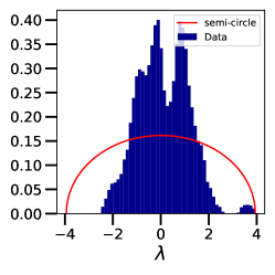
(a)

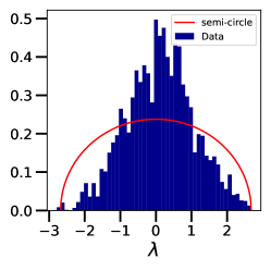
(b)

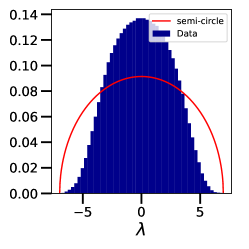
(c)

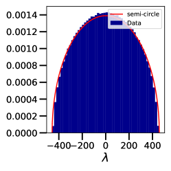
(d)

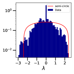
(e)

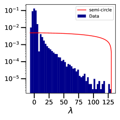
(f)

Figure 5: Spectral densities of Gaussian process Hessians with various kernel choices. All use $k^{\prime}(0)=1$. The dimension is $300$ in all cases except (d), in which the Hessian is padded to 400 dimensions with zeros. All histograms are produced with 100 independent Hessian samples. $*=100$ degenerate directions. $\dagger=20$ outliers

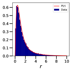
(a)

(b)

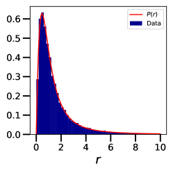
(c)

(d)

(e)

(f)

Figure 6: Consecutive spacing ratios of Gaussian process Hessians with various kernel choices. All use $k^{\prime}(0)=1$. The dimension is $300$ in all cases except (d), in which the Hessian is padded to 400 dimensions with zeros. $*=100$ degenerate directions. $\dagger=20$ outliers.

6.2 Beyond the MLP

Figure 7 shows the mean spectral density and adjacent spacing ratios for the Hessian of a CNN trained on CIFAR10. As with the MLP networks and MNIST data considered above, we see an obviously non-semicircular mean level density but the adjacent spacing ratios are nevertheless described by the universal GOE law.

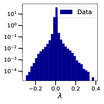
(a)

(b)

Figure 7: Spectral statistics for the Hessian of a CNN trained on CIFAR10. Hessians computed over batches of size 64 on the test set.

6.3 Beyond image classification

Figure 8 shows the mean spectral density and adjacent spacing ratios for the Hessian of an MLP trained on the Bike dataset. Once again we see an obviously non-semicircular mean level density but the adjacent spacing ratios are nevertheless described by the universal GOE law. This serves to demonstrate that there is nothing special about image data or, more importantly, high input feature dimension, since the Bike dataset has only 13 input features.

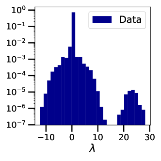
(a)

(b)

Figure 8: Spectral statistics for the Hessian of an MLP trained on the Bike dataset. Hessians computed over batches of size 64 on the test set.

6.4 Beyond the Hessian

Given that the Hessian is not the only matrix of interest in Machine Learning, it is pertinent to study whether our empirical results hold more generally. There have been lots of investigations for the Gauss-Newton [49, 63], or generalised Gauss-Newton (which is the analogue of the Gauss-Newton when using the cross entropy instead of square loss) matrices, particularly in the fields of optimisation [24, 54, 53, 52]. We consider the Gauss-Newton of the network trained on the Bike dataset with square loss. In this case the Gauss Newton $\mathbb{G}=\mathbb{J^{T}}\mathbb{J}$ shares the same non-null subspace as the Neural Tangent Kernel (NTK) [45, 19], where $\mathbb{J}$ denotes the Jacobian, i.e the derivative of the output with respect to the weights, which in this case is simply a vector. The NTK is used for the analysis of trajectories of gradient descent and is particularly interesting for large width networks, where it can be analytically shown that weights remain close to their initialisation and the network is well approximated by its linearisation. Figure 9 shows the mean spectral density and adjacent spacing ratios for the Gauss-Newton matrix of an MLP trained on the Bike dataset. The results are just as for the Hessians above: universal GOE spacings, but the mean density is very much not semicircular. This is an interesting result because even for a different matrix employed in a different context we still see the same universal RMT spacings.

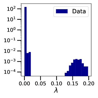
(a)

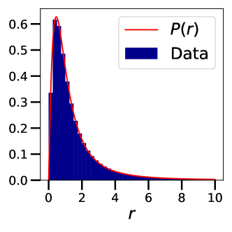
(b)

Figure 9: Spectral statistics for the Gauss-Newton matrix of an MLP trained on the Bike dataset. Matrices computed over batches of size 64 on the test set.

7 Conclusion and future work

We have demonstrated experimentally the existence of random matrix statistics in small neural networks on the scale of the mean eigenvalue separation. This provides the first direct evidence of universal RMT statistics present in neural networks trained on real datasets. Hitherto the role of random matrix theory in deep learning has been unclear. Prior work has studied theoretical models with specific assumptions leading to specific random matrix ensembles. Though certainly insightful, it is not clear to what extent any of these studies are applicable to real neural networks. This work aims to shift the focus by demonstrating the clear presence of universal random matrix behaviour in real neural networks. We expect that future theoretical studies will start from this robust supposition.

When working with a neural network on some dataset, one has information a priori about its Hessian. Its distribution and correlation structure may well be entirely inaccessible, but correlations between Hessian eigenvalues on the local scale can be assumed to be universal and overall the matrix can be rightly viewed as a random matrix possessing universal local statistics.

We focus on small neural networks where Hessian eigendecomposition is feasible. Future research that our work motivates could develop methods to approximate the level spacing distribution of large deep neural networks for which exact Hessian spectra cannot be computed. If the same RMT statistics are found, this would constitute a profound universal property of neural networks models; conversely, a break-down in these RMT statistics would be an indication of some fundamental separation between different network sizes or architectures.

A few recent works [50, 37, 2] considered and used the idea of Gaussian equivalence to make theoretical progress in neural network models with fewer assumptions than previously required (e.g. on the data distribution). The principle is that complicated random matrix distributions on non-linear functions of random matrices can be replaced in calculations training and test loss by their Gaussian equivalents, i.e. Gaussian matrices with matching first and second moments. This idea reflects a form of universality and can drastically increase the tractability of calculations. The random matrix universality we have here demonstrated in neural networks may be related, and should be considered as a possible source of other analogous universality simplifications that can render realistic but intractable models tractable.

One intriguing possible avenue is the relation to chaotic systems. Quantum systems with chaotic classical limits are know to display RMT spectral pairwise correlations, whereas Poisson statistics correspond to integrable systems. We suggest that the presence of GOE pairwise correlations in neural network Hessians, as opposed to Poisson, indicates that neural network training dynamics cannot be reduced to some simpler, smaller set of dynamical equations.

Appendix A Extra Figures and Degeneracy Investigation

Figure 14 compares the effect of degeneracy on unfolded spacings in each of the 3 cases considered. We see that the logistic MNIST models (trained and untrained) have a much greater level of degeneracy, whereas the CIFAR10-Resnet34 spectra clearly have GOE spacings even without any cut-off. Figures 11–13 show further unfolded spacing and spacing ratio results like those in the main text.

(a)

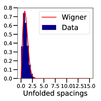
(b)

Figure 10: Unfolded spacings for the Hessian of a logistic regression trained on MNIST. Hessian computed batches of size 64 of the training and test datasets.

(a)

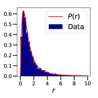
(b)

Figure 11: Consecutive spacing ratios for the Hessian of a logistic regression trained on MNIST. Hessian computed batches of size 64 of the training and test sets, and over the whole train and test sets.

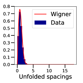
(a)

(b)

Figure 12: Unfolded spacings for the Hessian of a randomly initialised logistic regression for MNIST. Hessian computed batches of size 64 of the training and test datasets.

(a)

(b)

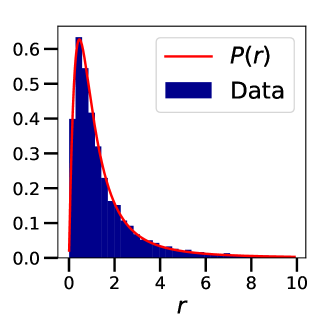
(c)

(d)

Figure 13: Consecutive spacing ratios for the Hessian of a randomly initialised logistic regression for MNIST. Hessian computed batches of size 64 of the training and test sets, and over the whole train and test sets.

(a)

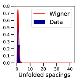
(b)

(c)

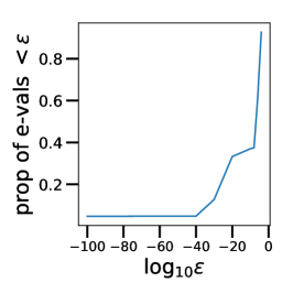
(d)

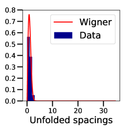
(e)

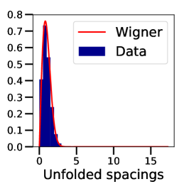
(f)

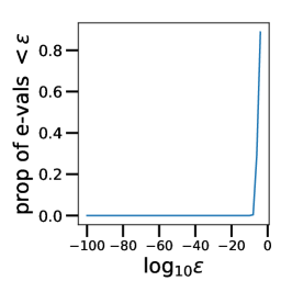
(g)

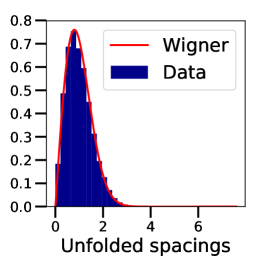
(h)

(i)

Figure 14: Unfolded spacings for the Hessian of a logistic regression. Showing MNIST (top), untrained MNIST (middle) and Resnet34 embedded CIFAR10 (bottom). Comparing the effect of a cuff-off for very small eigenvalues.

Appendix B Experimental details

B.1 Network architectures

Logistic regression (MNIST)

1. Input features 784 to 10 output logits.

2-layer MLP (MNIST)

1. Input features 784 to 10 neurons.

2. 10 neurons to 100 neurons.

3. 100 neurons to 10 output logits.

3-layer MLP (MNIST)

1. Input features 784 to 10 neurons.

2. 10 neurons to 100 neurons.

3. 100 neurons to 100 neurons.

4. 100 neurons to 10 output logits.

Logistic regression on ResNet features (CIFAR10)

1. Input features 513 to 10 neurons.

LeNet (CIFAR10)

1. Input features 32x32x3 through 5x5 convolution to 6 output channels.

2. 2x2 max pooling of stride 2.

3. 5x5 convolution to 16 output channels.

4. 2x2 max pooling of stride 2.

5. Fully connection layer from 400 to 120.

6. Fully connection layer from 120 to 84.

7. Fully connection layer from 84 to output 10 logits.

MLP (CIFAR10)

1. 3072 input features to 10 neurons.

2. 10 neurons to 300 neurons.

3. 300 neurons to 100 neurons.

MLP (Bike)

1. 13 input features to 100 neurons.

2. 100 neurons to 100 neurons.

3. 100 neurons to 50 neurons.

4. 50 neurons to 1 regression output.

B.2 Other details

All networks use the same (default) initialisation of weights in PyTorch, which is the ‘Kaiming uniform’ method of [43]. All networks used ReLU activation functions.

B.3 Data pre-processing

For the image datasets MNIST and CIFAR10 we use standard computer vision pre-processing, namely mean and variance standardisation across channels. We refer to the accompanying code for the precise procedure

The Bike dataset has 17 variables in total, namely: instant, dteday, season, yr, mnth, hr, holiday, weekday, workingday, weathersit, temp, atemp, hum, windspeed, casual, registered, cnt. All variables are either positive integers or real numbers. It is standard to view cnt as the regressand, so one uses some or all of the remaining features to predict cnt. This is the approach we take, however we slightly reduce the number of features by dropping instant, casual, registered, since instant is just an index and casual+registered=cnt, so including those features would render the problem trivial. We map dteday to a integer uniquely representing the date and we standardise cnt by dividing by its mean.

References

- Abuelenin and Abul-Magd [2012] Sherif M Abuelenin and Adel Y Abul-Magd. Effect of unfolding on the spectral statistics of adjacency matrices of complex networks. Procedia Computer Science, 12:69–74, 2012.
- Adlam and Pennington [2020] Ben Adlam and Jeffrey Pennington. The neural tangent kernel in high dimensions: Triple descent and a multi-scale theory of generalization. In International Conference on Machine Learning, pages 74–84. PMLR, 2020.
- Adler and Taylor [2009] Robert J Adler and Jonathan E Taylor. Random fields and geometry. Springer Science & Business Media, 2009.
- Amit et al. [1985] Daniel J Amit, Hanoch Gutfreund, and Haim Sompolinsky. Spin-glass models of neural networks. Physical Review A, 32(2):1007, 1985.
- Atas et al. [2013] YY Atas, E Bogomolny, O Giraud, and G Roux. Distribution of the ratio of consecutive level spacings in random matrix ensembles. Physical review letters, 110(8):084101, 2013.
- Auffinger et al. [2013] Antonio Auffinger, Gérard Ben Arous, and Jiří Černỳ. Random matrices and complexity of spin glasses. Communications on Pure and Applied Mathematics, 66(2):165–201, 2013.
- Ba et al. [2020] Jimmy Ba, Murat A Erdogdu, Taiji Suzuki, Denny Wu, and Tianzong Zhang. Generalization of two-layer neural net-works: An asymptotic viewpoint. risk, 1(1.5):2–0, 2020.
- Bahri et al. [2020] Yasaman Bahri, Jonathan Kadmon, Jeffrey Pennington, Sam S Schoenholz, Jascha Sohl-Dickstein, and Surya Ganguli. Statistical mechanics of deep learning. Annual Review of Condensed Matter Physics, 2020.
- Baskerville et al. [2021a] Nicholas P Baskerville, Jonathan P Keating, Francesco Mezzadri, and Joseph Najnudel. The loss surfaces of neural networks with general activation functions. Journal of Statistical Mechanics: Theory and Experiment, 2021(6):064001, 2021a.
- Baskerville et al. [2021b] Nicholas P Baskerville, Jonathan P Keating, Francesco Mezzadri, and Joseph Najnudel. A spin-glass model for the loss surfaces of generative adversarial networks. arXiv preprint arXiv:2101.02524, 2021b.
- Beenakker [1997] Carlo WJ Beenakker. Random-matrix theory of quantum transport. Reviews of modern physics, 69(3):731, 1997.
- Benigni and Péché [2019] Lucas Benigni and Sandrine Péché. Eigenvalue distribution of nonlinear models of random matrices. arXiv preprint arXiv:1904.03090, 2019.
- Berry and Robnik [1984] Michael V Berry and Marko Robnik. Semiclassical level spacings when regular and chaotic orbits coexist. Journal of Physics A: Mathematical and General, 17(12):2413, 1984.
- Berry et al. [1987] Michael V Berry et al. Quantum chaology. Proc. Roy. Soc. London A, 413:183–198, 1987.
- Berry and Tabor [1977] Michael Victor Berry and Michael Tabor. Level clustering in the regular spectrum. Proceedings of the Royal Society of London. A. Mathematical and Physical Sciences, 356(1686):375–394, 1977.
- Bohigas [1991] Oriol Bohigas. Random matrix theories and chaotic dynamics. Technical report, Paris-11 Univ., 1991.
- Bottou [2012] Léon Bottou. Stochastic Gradient Descent Tricks, pages 421–436. Springer Berlin Heidelberg, Berlin, Heidelberg, 2012. ISBN 978-3-642-35289-8. doi: 10.1007/978-3-642-35289-8˙25. URL https://doi.org/10.1007/978-3-642-35289-8_25.
- Bun et al. [2017] Joël Bun, Jean-Philippe Bouchaud, and Marc Potters. Cleaning large correlation matrices: tools from random matrix theory. Physics Reports, 666:1–109, 2017.
- Cai et al. [2019] Tianle Cai, Ruiqi Gao, Jikai Hou, Siyu Chen, Dong Wang, Di He, Zhihua Zhang, and Liwei Wang. Gram-gauss-newton method: Learning overparameterized neural networks for regression problems. arXiv preprint arXiv:1905.11675, 2019.
- Carleo et al. [2019] Giuseppe Carleo, Ignacio Cirac, Kyle Cranmer, Laurent Daudet, Maria Schuld, Naftali Tishby, Leslie Vogt-Maranto, and Lenka Zdeborová. Machine learning and the physical sciences. Reviews of Modern Physics, 91(4):045002, 2019.
- Chaudhari and Soatto [2015] Pratik Chaudhari and Stefano Soatto. On the energy landscape of deep networks. arXiv preprint arXiv:1511.06485, 2015.
- Choromanska et al. [2015a] Anna Choromanska, Mikael Henaff, Michael Mathieu, Gérard Ben Arous, and Yann LeCun. The loss surfaces of multilayer networks. In Artificial Intelligence and Statistics, pages 192–204, 2015a.
- Choromanska et al. [2015b] Anna Choromanska, Yann LeCun, and Gérard Ben Arous. Open problem: The landscape of the loss surfaces of multilayer networks. In Conference on Learning Theory, pages 1756–1760, 2015b.
- Dauphin et al. [2014] Yann N Dauphin, Razvan Pascanu, Caglar Gulcehre, Kyunghyun Cho, Surya Ganguli, and Yoshua Bengio. Identifying and attacking the saddle point problem in high-dimensional non-convex optimization. In Advances in neural information processing systems, pages 2933–2941, 2014.
- Deng [2012] Li Deng. The mnist database of handwritten digit images for machine learning research [best of the web]. IEEE Signal Processing Magazine, 29(6):141–142, 2012.
- Dhifallah and Lu [2020] Oussama Dhifallah and Yue M Lu. A precise performance analysis of learning with random features. arXiv preprint arXiv:2008.11904, 2020.
- Duchi et al. [2011] John Duchi, Elad Hazan, and Yoram Singer. Adaptive subgradient methods for online learning and stochastic optimization. Journal of machine learning research, 12(Jul):2121–2159, 2011.
- Efetov [1999] Konstantin Efetov. Supersymmetry in disorder and chaos. Cambridge university press, 1999.
- Fyodorov [2004] Yan V Fyodorov. Complexity of random energy landscapes, glass transition, and absolute value of the spectral determinant of random matrices. Physical review letters, 92(24):240601, 2004.
- Fyodorov and Le Doussal [2014] Yan V Fyodorov and Pierre Le Doussal. Topology trivialization and large deviations for the minimum in the simplest random optimization. Journal of Statistical Physics, 154(1):466–490, 2014.
- Fyodorov and Le Doussal [2018] Yan V Fyodorov and Pierre Le Doussal. Hessian spectrum at the global minimum of high-dimensional random landscapes. Journal of Physics A: Mathematical and Theoretical, 51(47):474002, 2018.
- Fyodorov and Williams [2007] Yan V Fyodorov and Ian Williams. Replica symmetry breaking condition exposed by random matrix calculation of landscape complexity. Journal of Statistical Physics, 129(5-6):1081–1116, 2007.
- Gabrié [2020] Marylou Gabrié. Mean-field inference methods for neural networks. Journal of Physics A: Mathematical and Theoretical, 53(22):223002, 2020.
- Gardner and Derrida [1988] Elizabeth Gardner and Bernard Derrida. Optimal storage properties of neural network models. Journal of Physics A: Mathematical and general, 21(1):271, 1988.
- Gerace et al. [2020] Federica Gerace, Bruno Loureiro, Florent Krzakala, Marc Mézard, and Lenka Zdeborová. Generalisation error in learning with random features and the hidden manifold model. In International Conference on Machine Learning, pages 3452–3462. PMLR, 2020.
- Ghorbani et al. [2019] Behrooz Ghorbani, Shankar Krishnan, and Ying Xiao. An investigation into neural net optimization via Hessian eigenvalue density. arXiv preprint arXiv:1901.10159, 2019.
- Goldt et al. [2020] Sebastian Goldt, Bruno Loureiro, Galen Reeves, Florent Krzakala, Marc Mézard, and Lenka Zdeborová. The gaussian equivalence of generative models for learning with shallow neural networks. arXiv preprint arXiv:2006.14709, 2020.
- Granziol [2020] Diego Granziol. Beyond random matrix theory for deep networks. arXiv preprint arXiv:2006.07721, 2020.
- Granziol et al. [2019a] Diego Granziol, Timur Garipov, Dmitry Vetrov, Stefan Zohren, Stephen Roberts, and Andrew Gordon Wilson. Towards understanding the true loss surface of deep neural networks using random matrix theory and iterative spectral methods. 2019a.
- Granziol et al. [2019b] Diego Granziol, Xingchen Wan, Timur Garipov, Dmitry Vetrov, and Stephen Roberts. MLRG deep curvature. arXiv preprint arXiv:1912.09656, 2019b.
- Granziol et al. [2020] Diego Granziol, Timur Garipov, Dmitry Vetrov, Stefan Zohren, Stephen Roberts, and Andrew Gordon Wilson. Towards understanding the true loss surface of deep neural networks using random matrix theory and iterative spectral methods. https://openreview.net/forum?id=H1gza2NtwH, 2020.
- Guhr et al. [1998] Thomas Guhr, Axel Müller-Groeling, and Hans A Weidenmüller. Random-matrix theories in quantum physics: common concepts. Physics Reports, 299(4-6):189–425, 1998.
- He et al. [2015] Kaiming He, Xiangyu Zhang, Shaoqing Ren, and Jian Sun. Delving deep into rectifiers: Surpassing human-level performance on imagenet classification. In Proceedings of the IEEE international conference on computer vision, pages 1026–1034, 2015.
- He et al. [2016] Kaiming He, Xiangyu Zhang, Shaoqing Ren, and Jian Sun. Deep residual learning for image recognition. In Proceedings of the IEEE conference on computer vision and pattern recognition, pages 770–778, 2016.
- Jacot et al. [2018] Arthur Jacot, Franck Gabriel, and Clément Hongler. Neural tangent kernel: Convergence and generalization in neural networks. arXiv preprint arXiv:1806.07572, 2018.
- Kingma and Ba [2014] Diederik P Kingma and Jimmy Ba. Adam: A method for stochastic optimization. arXiv preprint arXiv:1412.6980, 2014.
- Krizhevsky et al. [2009] Alex Krizhevsky, Geoffrey Hinton, et al. Learning multiple layers of features from tiny images. 2009.
- LeCun [1998] Yann LeCun. The MNIST database of handwritten digits. http://yann. lecun. com/exdb/mnist/, 1998.
- Loke and Dahlin [2002] Meng Heng Loke and Torleif Dahlin. A comparison of the gauss–newton and quasi-newton methods in resistivity imaging inversion. Journal of applied geophysics, 49(3):149–162, 2002.
- Loureiro et al. [2021] Bruno Loureiro, Cédric Gerbelot, Hugo Cui, Sebastian Goldt, Florent Krzakala, Marc Mézard, and Lenka Zdeborová. Capturing the learning curves of generic features maps for realistic data sets with a teacher-student model. arXiv preprint arXiv:2102.08127, 2021.
- Maillard et al. [2020] Antoine Maillard, Gérard Ben Arous, and Giulio Biroli. Landscape complexity for the empirical risk of generalized linear models. In Mathematical and Scientific Machine Learning, pages 287–327. PMLR, 2020.
- Martens [2014] James Martens. New insights and perspectives on the natural gradient method. arXiv preprint arXiv:1412.1193, 2014.
- Martens and Grosse [2015] James Martens and Roger Grosse. Optimizing neural networks with Kronecker-factored approximate curvature. In International conference on machine learning, pages 2408–2417, 2015.
- Martens and Sutskever [2012] James Martens and Ilya Sutskever. Training deep and recurrent networks with Hessian-free optimization. In Neural networks: Tricks of the trade, pages 479–535. Springer, 2012.
- Mehta [2004] Madan Lal Mehta. Random matrices. Elsevier, 2004.
- Mei and Montanari [2019] Song Mei and Andrea Montanari. The generalization error of random features regression: Precise asymptotics and the double descent curve. Communications on Pure and Applied Mathematics, 2019.
- Meurant and Strakoš [2006] Gérard Meurant and Zdeněk Strakoš. The Lanczos and conjugate gradient algorithms in finite precision arithmetic. Acta Numerica, 15:471–542, 2006.
- Mezard and Montanari [2009] Marc Mezard and Andrea Montanari. Information, physics, and computation. Oxford University Press, 2009.
- Papyan [2018] Vardan Papyan. The full spectrum of deepnet hessians at scale: Dynamics with sgd training and sample size. arXiv preprint arXiv:1811.07062, 2018.
- Papyan [2019] Vardan Papyan. Measurements of three-level hierarchical structure in the outliers in the spectrum of deepnet hessians. arXiv preprint arXiv:1901.08244, 2019.
- Paszke et al. [2017] Adam Paszke, Sam Gross, Soumith Chintala, Gregory Chanan, Edward Yang, Zachary DeVito, Zeming Lin, Alban Desmaison, Luca Antiga, and Adam Lerer. Automatic differentiation in Pytorch. 2017.
- Pearlmutter [1994] Barak A Pearlmutter. Fast exact multiplication by the Hessian. Neural computation, 6(1):147–160, 1994.
- Pennington and Bahri [2017] Jeffrey Pennington and Yasaman Bahri. Geometry of neural network loss surfaces via random matrix theory. In Proceedings of the 34th International Conference on Machine Learning-Volume 70, pages 2798–2806. JMLR. org, 2017.
- Pennington and Worah [2018] Jeffrey Pennington and Pratik Worah. The spectrum of the fisher information matrix of a single-hidden-layer neural network. In S. Bengio, H. Wallach, H. Larochelle, K. Grauman, N. Cesa-Bianchi, and R. Garnett, editors, Advances in Neural Information Processing Systems 31, pages 5410–5419. Curran Associates, Inc., 2018.
- Pennington and Worah [2019] Jeffrey Pennington and Pratik Worah. Nonlinear random matrix theory for deep learning. Journal of Statistical Mechanics: Theory and Experiment, 2019(12):124005, 2019.
- PyTorch [2021] PyTorch. Resnet. https://pytorch.org/hub/pytorch_vision_resnet, 2021. Accessed: 2021-05-03.
- Roberts et al. [2021] Daniel A Roberts, Sho Yaida, and Boris Hanin. The principles of deep learning theory. arXiv preprint arXiv:2106.10165, 2021.
- Ros et al. [2019] Valentina Ros, Gerard Ben Arous, Giulio Biroli, and Chiara Cammarota. Complex energy landscapes in spiked-tensor and simple glassy models: Ruggedness, arrangements of local minima, and phase transitions. Physical Review X, 9(1):011003, 2019.
- Sagun et al. [2014] Levent Sagun, V Ugur Guney, Gerard Ben Arous, and Yann LeCun. Explorations on high dimensional landscapes. arXiv preprint arXiv:1412.6615, 2014.
- Sagun et al. [2016] Levent Sagun, Léon Bottou, and Yann LeCun. Eigenvalues of the Hessian in deep learning: Singularity and beyond. arXiv preprint arXiv:1611.07476, 2016.
- Sagun et al. [2017] Levent Sagun, Utku Evci, V Ugur Guney, Yann Dauphin, and Leon Bottou. Empirical analysis of the Hessian of over-parametrized neural networks. arXiv preprint arXiv:1706.04454, 2017.
- Sarao Mannelli et al. [2019] Stefano Sarao Mannelli, Giulio Biroli, Chiara Cammarota, Florent Krzakala, and Lenka Zdeborová. Who is afraid of big bad minima? analysis of gradient-flow in spiked matrix-tensor models. In H. Wallach, H. Larochelle, A. Beygelzimer, F. d'Alché-Buc, E. Fox, and R. Garnett, editors, Advances in Neural Information Processing Systems, volume 32. Curran Associates, Inc., 2019. URL https://proceedings.neurips.cc/paper/2019/file/fbad540b2f3b5638a9be9aa6a4d8e450-Paper.pdf.
- Scholak [2015] Torsten Scholak. unfoldr. https://github.com/tscholak/unfoldr, 2015. Accessed: 2020-10-30.
- Scholak et al. [2014] Torsten Scholak, Thomas Wellens, and Andreas Buchleitner. Spectral backbone of excitation transport in ultracold rydberg gases. Physical Review A, 90(6):063415, 2014.
- Sharif Razavian et al. [2014] Ali Sharif Razavian, Hossein Azizpour, Josephine Sullivan, and Stefan Carlsson. Cnn features off-the-shelf: an astounding baseline for recognition. In Proceedings of the IEEE conference on computer vision and pattern recognition workshops, pages 806–813, 2014.
- Tao [2012] Terence Tao. Topics in random matrix theory, volume 132. American Mathematical Soc., 2012.
- Wang et al. [2019] Ke Wang, Geoff Pleiss, Jacob Gardner, Stephen Tyree, Kilian Q Weinberger, and Andrew Gordon Wilson. Exact gaussian processes on a million data points. Advances in Neural Information Processing Systems, 32:14648–14659, 2019.
- Weidenmuller and Mitchell [2008] HA Weidenmuller and GE Mitchell. Random matrices and chaos in nuclear physics. arXiv preprint arXiv:0807.1070, 2008.
- Zdeborová and Krzakala [2016] Lenka Zdeborová and Florent Krzakala. Statistical physics of inference: Thresholds and algorithms. Advances in Physics, 65(5):453–552, 2016.