Atom-dimer and dimer-dimer scatterings in a spin-orbit coupled Fermi gas

Abstract

Using the diagrammatic approach, here we study how spin-orbit coupling (SOC) affects the fermion-dimer and dimer-dimer scattering lengths in the Born approximation, and benchmark their accuracy with the higher-order approximations. We consider both isotropic and Rashba couplings in three dimensions, and show that the Born approximation gives accurate results in the $1/(m\alpha a_{s})\ll-1$ limit, where $m$ is the mass of the fermions, $\alpha$ is the strength of the SOC, and $a_{s}$ is the $s$-wave scattering length between fermions. This is because the higher-loop contributions form a perturbative series in the $1/(m\alpha a_{s})<0$ region that is controlled by the smallness of the residue $Z$ of the dimer propagator. In sharp contrast, since $Z$ grows with the square-root of the binding energy of the dimer in the $1/(m\alpha a_{s})>0$ region, all of the higher-loop contributions are of similar order.

I Introduction

The diagrammatic approach has proven to be a powerful technique for studying few-body problems in many branches of theoretical physics. For instance, in the context of short-range two-body interactions between particles, it has been successfully applied to both the three-body bedaque98 ; brodsky06 ; levinsen06 ; iskin08 ; iskin10 ; alzetto10 ; levinsen11 and four-body pieri00 ; brodsky06 ; levinsen06 ; alzetto13 problems to verify the known exact results for the fermion-dimer skorniakov57 ; petrov03 and dimer-dimer petrov05 scattering lengths, respectively. In addition, the approach have recently been generalized to the three-body problem with arbitrary-range two-body interactions, and applied to the electron-exciton scattering in semiconductors, i.e., to the so-called three-body Coulomb problem combescot17 .

Furthermore, in the context of BCS-BEC crossover strinati18 , the fermion-dimer and dimer-dimer scattering lengths appear in some of the many-body properties of dilute Fermi gases, including their low-energy collective modes, superfluid density, etc.. Such appearances are quite natural in those parameter regimes where a strongly interacting Fermi-Fermi mixture can be mapped to a weakly-interacting Bose-Fermi mixture of paired (i.e., bosonic dimers) and unpaired (i.e., excess) fermions pieri06 ; taylor07 ; iskin08 . However, it is also known that the usual treatment of the BCS-BEC crossover through a Gaussian fluctuation approach yields fermion-dimer and dimer-dimer scattering lengths that are consistent with the lowest-order Born approximation brodsky06 ; levinsen06 ; pieri00 .

Given the recent surge of experimental cheuk12 ; williams13 ; huang16 ; meng16 and theoretical zhai11 ; iskin11 ; hu11 ; he12a ; he12b ; shenoy12a ; shenoy12b interests in spin-orbit-coupled Fermi gases, here we extend the diagrammatic approach to the relevant few-body problems. In particular, we study how SOC affects the fermion-dimer and dimer-dimer scattering lengths in the Born approximation, and benchmark their accuracy with the higher-order approximations. Our primary findings for the isotropic and Rashba couplings in three dimensions are as follows. We show that the Born approximation gives accurate results in the $1/(m\alpha a_{s})\ll-1$ limit, as the higher-loop contributions form a perturbative series in the $1/(m\alpha a_{s})<0$ region that is controlled by the residue $Z$ of the dimer propagator. While $Z$ decays to $0$ in the $1/(m\alpha a_{s})\to-\infty$ limit, it grows with the square-root of the binding energy of the dimer in the $1/(m\alpha a_{s})>0$ region, suggesting that it may be sufficient to consider a finite number of higher-loop diagrams in the $1/(m\alpha a_{s})<0$ region.

The rest of the paper is organized as follows. In Sec. II, we introduce the one-body Hamiltonian, helicity bands and the fermion propagator. In Sec. III, we introduce the two-body Hamiltonian, identify the appropriate Feynman rules for the bound-state problem, and derive the dimer propagator for the composite bosons. In Sec. IV, we analyze the fermion-dimer scattering t-matrix, and extract the fermion-dimer scattering length in the zero-loop Born, one-loop and two-loop approximations. In Sec. V, we analyze the dimer-dimer scattering t-matrix, and extract the dimer-dimer scattering length in the one-loop Born and two-loop approximations. In Sec. VI, we discuss how the fermion-dimer and dimer-dimer scattering lengths are related to the many-body problem. In Sec. VII, we compare our findings for the isotropic SOC with those of the anisotropic (Rashba) SOC. The paper ends with a brief summary of our conclusions in Sec. VIII. For the sake of completeness, the binding energy and effective mass of the dimer are presented in the Appendix.

II One-body problem

In the $\langle\uparrow|=\begin{pmatrix}1&0\end{pmatrix}$ and $\langle\downarrow|=\begin{pmatrix}0&1\end{pmatrix}$ basis of the $\sigma_{z}$ Pauli matrix, the single-particle problem is governed by the Hamiltonian matrix

$$h_{\mathbf{k}}=\varepsilon_{\mathbf{k}}\sigma_{0}+\alpha\mathbf{k}\cdot\boldsymbol{\sigma}$$ (1)

in momentum space, where $\mathbf{k}=(k_{x},k_{y},k_{z})$ is the wave vector, $\varepsilon_{\mathbf{k}}=k^{2}/(2m)$ is the usual dispersion with $k=\sqrt{k_{x}^{2}+k_{y}^{2}+k_{z}^{2}}$ in units of $\hbar=1$, $\sigma_{0}$ is a unit matrix, $\alpha\geq 0$ is the strength of the SOC that is taken as an isotropic field in $\mathbf{k}$ space, and $\boldsymbol{\sigma}=(\sigma_{x},\sigma_{y},\sigma_{z})$ is a vector of Pauli matrices. The eigenvalues and eigenvectors of $h_{\mathbf{k}}$ are determined by the unitary transformation

$$U_{\mathbf{k}}=\frac{1}{\sqrt{2k(k-k_{z})}}\begin{pmatrix}k_{x}-ik_{y}&k_{z}-k\\ k-k_{z}&k_{x}+ik_{y}\end{pmatrix},$$ (2)

where $U_{\mathbf{k}}^{\dagger}h_{\mathbf{k}}U_{\mathbf{k}}$ gives the dispersion relations of the $s=\pm$ helicity bands

$$\varepsilon_{\mathbf{k}}^{s}=\frac{k^{2}}{2m}+s\alpha k,$$ (3)

and $U_{\mathbf{k}}|\uparrow(\downarrow)\rangle$ gives the corresponding eigenstates. We illustrate these dispersions in Fig. 1 as a function of $k$, and note that the ground state of the $-$-helicity band corresponds to a degenerate shell of $\mathbf{k}$ states with the radius $k_{m}=m\alpha$ and energy $\varepsilon_{\mathbf{k}_{m}}^{-}=-m\alpha^{2}/2$.

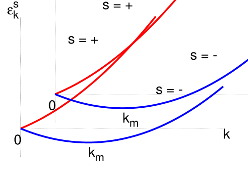
Figure 1: One-body dispersions $\varepsilon_{\mathbf{k}}^{s}=k^{2}/(2m)+s\alpha k$ for the $s=\pm$ helicity bands. The minimum of the lower band corresponds to a shell of $\mathbf{k}$ states with the radius $k_{m}=m\alpha$ and energy $\varepsilon_{\mathbf{k}_{m}}^{-}=-m\alpha^{2}/2$.

Given the Hamiltonian matrix in Eq. (1), the propagator of the single particle can be written as

$$G(\mathbf{k},k_{0})=\frac{1}{(k_{0}+i0^{+})\sigma_{0}-h_{\mathbf{k}}},$$ (4)

where $k_{0}$ is the energy, and we set the chemical potential $\mu$ to $0$ for the few-body problems of interest below. In our analysis, we reexpress such propagators via the generic relation $1/(A\sigma_{0}-\mathbf{B}\cdot\boldsymbol{\sigma})=(A\sigma_{0}+\mathbf{B}\cdot\boldsymbol{\sigma})/(A^{2}-B^{2})=(1/2)\sum_{s}(\sigma_{0}+s\widehat{\mathbf{B}}\cdot\boldsymbol{\sigma})/(A-sB),$ where $\widehat{\mathbf{B}}=\mathbf{B}/B$ and $B=|\mathbf{B}|$.

III Two-body problem

Having in mind the atomic Fermi gases where the bosonic dimer is a result of a short-range interaction between $\uparrow$ and $\downarrow$ fermions, our two-body interaction is governed by the Hamiltonian density

$$h_{\mathbf{r}}=-g\psi_{\uparrow}^{\dagger}(\mathbf{r})\psi_{\downarrow}^{\dagger}(\mathbf{r})\psi_{\downarrow}(\mathbf{r})\psi_{\uparrow}(\mathbf{r})$$ (5)

in real space, where $g\geq 0$ is the strength of the fermion-fermion attraction, and $\psi_{\sigma}^{\dagger}(\mathbf{r})$ and $\psi_{\sigma}(\mathbf{r})$ are the fermionic field operators. A convenient way to understand the action of this term is through a Hubbard-Stratonovich transformation in the imaginary-time functional path-integral formalism iskin11 ; hu11 ; he12a ; he12b ; shenoy12a ; shenoy12b . Introducing the Hubbard-Stratonovich fields $\Delta=-g\psi_{\downarrow}\psi_{\uparrow}$ and $\bar{\Delta}=-g\bar{\psi}_{\uparrow}\bar{\psi}_{\downarrow},$ where $\bar{\psi}_{\sigma}$and $\psi_{\sigma}$ are the corresponding Grassmann variables with suppressed arguments $x=(\mathbf{r},\tau)$ for notational simplicity, the action that corresponds to Eq. (5) is replaced by three terms $\bar{\Delta}\Delta/g+\Delta\bar{\psi}_{\uparrow}\bar{\psi}_{\downarrow}+\bar{\Delta}\psi_{\downarrow}\psi_{\uparrow}.$ If one interprets $\bar{\Delta}=\Delta^{*}$ as the complex dimer field then the first term describes free dimers with a bare propagator $-g$, and the second and third terms describe the dimer-fermion and fermion-dimer conversion processes, respectively.

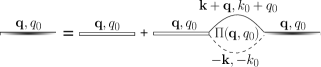
Figure 2: Diagrammatic representation of the two-body binding problem. The dimer propagator (colored bars) is determined by dressing its bare propagator (uncolored bars) with infinitely-many fermion-fermion bubbles (solid and dashed lines), forming eventually a geometric series.

The diagrammatic representation of the two-body binding problem in $\mathbf{k}$ space is shown in Fig. 2, where the physical dimer propagator $D(\mathbf{q},q_{0})$ is determined by dressing its bare value, which is a constant in space, with repeated interactions between its fermionic constituents brodsky06 ; levinsen06 . The resultant geometric series can be summed over to yield

$$D(\mathbf{q},q_{0})=\frac{-g}{1+g\Pi(\mathbf{q},q_{0})},$$ (6)

where $\Pi(\mathbf{q},q_{0})$ corresponds to the fermion-fermion bubble diagram that is given by

$$\Pi(\mathbf{q},q_{0})=\frac{\mathrm{Tr}}{2}\sum_{k}\sigma_{y}G(\mathbf{k}+\mathbf{q},k_{0}+q_{0})\sigma_{y}G^{\mathrm{T}}(-\mathbf{k},-k_{0}).$$ (7)

Here, $\mathrm{Tr}$ is a trace over the spin sector, and $\sum_{k}$ represents $\sum_{\mathbf{k},k_{0}}=i\int d^{3}\mathbf{k}\int dk_{0}/(2\pi)^{4}.$ In our diagrams, while the solid lines correspond to the fermion propagators that are described by Eq. (4), the dashed lines correspond to their dimer partners that are described by the transpose $\mathrm{T}$ of Eq. (4). This is because the dimer is formed between a particle that is governed by $h_{\mathbf{k}+\mathbf{q}}$ and a hole that is governed by $-h_{-\mathbf{k}}^{\mathrm{T}}$ in $\mathbf{k}$ space iskin11 ; hu11 ; he12a ; he12b ; shenoy12a ; shenoy12b . In accordance with the Feynman rules, each fermion line, dimer line and vertex carries a factor of $i$. In addition, we associate each dimer-creation (-annihilation) vertex with an additional factor of $\mp i\sigma_{y}$ to account for the fermion-dimer (dimer-fermion) conversion terms, i.e., $-i\bar{\Delta}\sigma_{y}$ and $i\Delta\sigma_{y}$, respectively, in the particle-hole sectors.

Noting the relation $\sigma_{y}\mathbf{B}\cdot\boldsymbol{\sigma}^{\mathrm{T}}\sigma_{y}=-\mathbf{B}\cdot\boldsymbol{\sigma},$ and integrating $k_{0}$ in the upper half plane in which there are two simple poles at $k_{0}=-\varepsilon_{\mathbf{k}}^{\pm}$, we find he12b

$$\Pi(\mathbf{q},q_{0})=\frac{1}{4}\sum_{ss^{\prime}\mathbf{k}}\frac{1+ss^{\prime}\widehat{\mathbf{k}}\cdot\widehat{\mathbf{Q}}}{q_{0}-\varepsilon_{\mathbf{k}}^{s}-\varepsilon_{\mathbf{Q}}^{s^{\prime}}},$$ (8)

where $\mathbf{Q}=\mathbf{k}+\mathbf{q}$. Equation (8) shows that only the intra-band processes contribute to the bubble diagram when the dimer is stationary, i.e., when its center-of-mass momentum $\mathbf{q}$ vanishes. Therefore, we can reexpress the stationary bubble diagram as $\Pi(\mathbf{0},q_{0})=(1/2)\sum_{sk}G_{s}(\mathbf{k},k_{0}+q_{0})G_{s}(-\mathbf{k},-k_{0}),$ where

$$G_{s}(\mathbf{k},k_{0})=\frac{1}{k_{0}-\varepsilon_{\mathbf{k}}^{s}+i0^{+}}$$ (9)

is the fermion propagator in the $s=\pm$ helicity basis.

In the lowest order in $\mathbf{q}$ and $q_{0}$, Eq. (6) has the generic structure of a simple pole iskin11 ; hu11 ; he12a ; he12b ; shenoy12a ; shenoy12b

$$D(\mathbf{q},q_{0})=\frac{Z}{q_{0}-q^{2}/(2m_{B})+\mu_{B}+i0^{+}}$$ (10)

where $Z=8\pi(|\varepsilon_{b}|-m\alpha^{2})^{3/2}/(m\sqrt{m}|\varepsilon_{b}|)$ corresponds to the residue of the pole, $2m/m_{B}=7/3-4(1-m\alpha^{2}/|\varepsilon_{b}|)^{3/2}/3-2m\alpha^{2}/|\varepsilon_{b}|$ determines the effective mass of the bosonic dimer, and $\mu_{B}=2\mu-\varepsilon_{b}\to-\varepsilon_{b}$ corresponds to its chemical potential. Noting that $-m\alpha^{2}$ is the two-body continuum threshold, the energy of the two-body bound state $\varepsilon_{b}\leq-m\alpha^{2}$ or the two-body binding energy $|\varepsilon_{b}|-m\alpha^{2}$ of the dimer can be simply found by looking at the pole of $D(\mathbf{0},\varepsilon_{b})$, leading to the relation $1=(g/2)\sum_{s\mathbf{k}}1/(2\varepsilon_{\mathbf{k}}^{s}-\varepsilon_{b}).$ In addition, we substitute $g$ with the usual t-matrix relation between two fermions in vacuum without the SOC, $1/g=-mV/(4\pi a_{s})+\sum_{\mathbf{k}}1/(2\varepsilon_{\mathbf{k}}),$ where $\sum_{\mathbf{k}}=V\int d^{3}\mathbf{k}/(2\pi)^{3}$ in units of $V=1$. This leads to $\varepsilon_{b}=-2m\alpha^{2}-1/(2ma_{s}^{2})\pm\sqrt{1/(4m^{2}a_{s}^{4})+\alpha^{2}/a_{s}^{2}}$ for $a_{s}\lessgtr 0$, showing that $\varepsilon_{b}\leq-m\alpha^{2}$ for all parameters. This expression is analytically tractable in three limits iskin11 ; he12b ; shenoy12a ; shenoy12b : we find that (i) $\varepsilon_{b}=-m\alpha^{2}-m^{3}\alpha^{4}a_{s}^{2}$ and $m_{B}=6m$ in the limit when $1/(m\alpha a_{s})\ll-1$, (ii) $\varepsilon_{b}=-2m\alpha^{2}$ and $m_{B}=3\sqrt{2}/(2\sqrt{2}-1)m\approx 2.32m$ in the unitarity limit when $1/(m\alpha a_{s})=0$, and (iii) $\varepsilon_{b}=-1/(ma_{s}^{2})$ and $m_{B}=2m$ in the limit when $1/(m\alpha a_{s})\gg 1$. These results are illustrated in Fig. 10 for the completeness of the presentation. Note that the latter limit recovers the usual two-body problem with no SOC in the $1/(m\alpha a_{s})\gg 1$ limit when $\alpha\to 0^{+}$.

IV Three-body problem

In this section, we are interested in the scattering t-matrix $t_{k}^{--}(0)$ between the lowest-energy fermion in the $-$-helicity band and a stationary dimer. For this purpose, we introduce a shorthand notation

$$\mathcal{T}_{k}(p)=\begin{bmatrix}t_{k}^{\uparrow\uparrow}(p)&t_{k}^{\uparrow\downarrow}(p)\\ t_{k}^{\downarrow\uparrow}(p)&t_{k}^{\downarrow\downarrow}(p)\end{bmatrix},$$ (11)

where $k=({\mathbf{k},k_{0}})$ refers collectively to the momentum and energy of the incoming fermion, and $p=({\mathbf{p},p_{0}})$ refers collectively to the momentum and energy exchange between the outgoing fermion and the dimer. We refer to Fig. 5 for the clarity of its meaning. Once $\mathcal{T}_{k}(0)$ is evaluated, we transform it to the helicity basis via Eq. (2), and obtain $U_{\mathbf{k}}^{\dagger}\mathcal{T}_{k}(0)U_{\mathbf{k}}.$ Using the spherical coordinates where $\widehat{\mathbf{k}}=(\sin\theta_{\mathbf{k}}\cos\phi_{\mathbf{k}},\sin\theta_{\mathbf{k}}\sin\phi_{\mathbf{k}},\cos\theta_{\mathbf{k}}),$ we find

$$t_{k}^{ss}(0) =t_{k}^{\uparrow\uparrow}(0)\frac{1+s\cos\theta_{\mathbf{k}}}{2}+t_{k}^{\downarrow\downarrow}(0)\frac{1-s\cos\theta_{\mathbf{k}}}{2}$$

$$+s\mathrm{Re}[t_{k}^{\uparrow\downarrow}(0)\sin\theta_{\mathbf{k}}(\cos\phi_{\mathbf{k}}+i\sin\phi_{\mathbf{k}})]$$ (12)

for the diagonal elements with $\mathrm{Re}$ the real part. Note in particular that $t_{k}^{--}(0)=t_{k}^{\downarrow\downarrow}(0)$ for $\mathbf{k}$ that is aligned with the $z$ axis, i.e., when $\theta_{\mathbf{k}}=0$. In this paper, we are interested in the fermion-dimer scattering length $a_{BF}$ that is determined by brodsky06 ; levinsen06

$$a_{BF}=\frac{m_{BF}}{4\pi}Zt_{k}^{--}(0),$$ (13)

where $m_{BF}=2m_{B}m_{F}/(m_{B}+m_{F})$ is twice the reduced mass of the fermion and the dimer, and $k=(m\alpha\widehat{\mathbf{k}},-m\alpha^{2}/2)$ corresponds to the lowest-energy eigenstate in the $-$-helicity band.

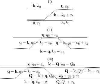
Figure 3: Diagrammatic representations of the (i) zero-loop Born, (ii) one-loop and (iii) two-loop contributions to the fermion-dimer scattering t-matrix.

For instance, the diagrammatic representations of the zero-loop, one-loop and two-loop contributions to the fermion-dimer scattering t-matrix are shown in Fig. 3 bedaque98 ; brodsky06 ; levinsen06 ; iskin08 ; iskin10 ; alzetto10 ; levinsen11 ; combescot17 . The zero-loop contribution is known as the Born approximation, and in accordance with the Feynman rules given above, it is given by

$$\mathcal{T}_{k}^{(0)}(0)=-\sigma_{y}G^{\mathrm{T}}(-\mathbf{k},-k_{0}+\varepsilon_{b})\sigma_{y},$$ (14)

where the minus sign is due to the exchange of an identical fermion. By plugging Eq. (14) into Eq. (12), we find

$${t_{k}^{ss}}^{(0)}(0)=\frac{1}{k_{0}-\varepsilon_{b}+\varepsilon_{\mathbf{k}}^{s}},$$ (15)

which is physically intuitive. This is because, since both dimers are stationary in the Born diagram, the helicity bands are not coupled, and $t_{k}^{ss}(0)$ can be directly expressed as ${t_{k}^{ss}}^{(0)}(0)=-G_{s}(-\mathbf{k},-k_{0}+\varepsilon_{b}).$ Furthermore, by plugging ${t_{k}^{--}}^{(0)}(0)=1/(|\varepsilon_{b}|-m\alpha^{2})$ into Eq. (13), we find

$$a_{BF}^{\mathrm{Born}}=\frac{2m_{BF}\sqrt{|\varepsilon_{b}|-m\alpha^{2}}}{m\sqrt{m}|\varepsilon_{b}|}$$ (16)

in the Born approximation, suggesting that the fermion-dimer interaction is repulsive for all parameters. In Fig. 4, we show $a_{BF}^{\mathrm{Born}}$ as a function of $1/(m\alpha a_{s})$, which is analytically tractable in three limits: (i) $a_{BF}^{\mathrm{Born}}=-24a_{s}/7$ in the limit when $1/(m\alpha a_{s})\ll-1$, (ii) $a_{BF}^{\mathrm{Born}}=6\sqrt{2}/[m\alpha(5\sqrt{2}-1)]\approx 1.40/(m\alpha)$ in the unitarity limit when $1/(m\alpha a_{s})=0$, and (iii) $a_{BF}^{\mathrm{Born}}=8a_{s}/3$ in the limit when $1/(m\alpha a_{s})\gg 1$. Note that the latter limit recovers the usual three-body problem with no SOC in the $1/(m\alpha a_{s})\gg 1$ limit when $\alpha\to 0^{+}$.

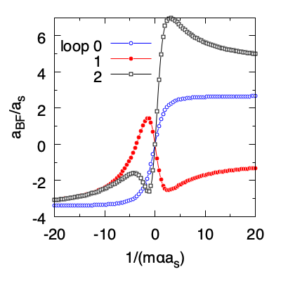
Figure 4: Fermion-dimer scattering length in the zero-loop Born, one-loop and two-loop approximations. The higher-loop contributions form a perturbative series in the $1/(m\alpha a_{s})<0$ region, but they are of similar order in the $1/(m\alpha a_{s})>0$ region.

To go beyond the Born approximation, we consider the one-loop contribution that is shown in Fig. 3(ii). In accordance with the Feynman rules, this diagram is given by

$$\mathcal{T}_{k}^{(1)}(0)=\sum_{q}\sigma_{y}G^{\mathrm{T}}(\mathbf{q}-\mathbf{k},q_{0}-k_{0}+\varepsilon_{b})\sigma_{y}D(\mathbf{q},q_{0}+\varepsilon_{b})$$

$$\times G(\mathbf{k}-\mathbf{q},k_{0}-q_{0})\sigma_{y}G^{\mathrm{T}}(\mathbf{q}-\mathbf{k},q_{0}-k_{0}+\varepsilon_{b})\sigma_{y}.$$ (17)

Noting the relation $(\sigma_{0}+\widehat{\mathbf{A}}\cdot\boldsymbol{\sigma})(\sigma_{0}+\widehat{\mathbf{B}}\cdot\boldsymbol{\sigma})=(1+\widehat{\mathbf{A}}\cdot\widehat{\mathbf{B}})\sigma_{0}+(\widehat{\mathbf{A}}+\widehat{\mathbf{B}}+i\widehat{\mathbf{A}}\times\widehat{\mathbf{B}})\cdot\boldsymbol{\sigma},$ we first integrate $q_{0}$ in the upper half plane in which there are two simple poles at $q_{0}=k_{0}-\varepsilon_{\mathbf{q}}^{\pm}$, and reduce the t-matrix contribution to

$$\mathcal{T}_{k}^{(1)}(0)=\frac{1}{2}\sum_{s\mathbf{q}}\frac{D(\mathbf{q}+\mathbf{k},k_{0}+\varepsilon_{b}-\varepsilon_{\mathbf{q}}^{s})}{(2\varepsilon_{\mathbf{q}}^{s}-\varepsilon_{b})^{2}}(\sigma_{0}-s\widehat{\mathbf{q}}\cdot\boldsymbol{\sigma}).$$ (18)

Noting that $\mathcal{T}_{k}(0)$ has a spherical symmetry in $\mathbf{k}$ space, we choose an incoming momentum $\mathbf{k}=m\alpha\widehat{k_{z}}$ that is aligned with the $z$ axis, and perform the remaining integrations numerically in the $\mathbf{q}$ space integralnote . In Fig. 4, we show how the one-loop contribution affects $a_{BF}^{\mathrm{Born}}$ as a function of $1/(m\alpha a_{s})$. In the one-loop approximation, we find that $a_{BF}^{\mathrm{Born}}$ becomes attractive in the $1/(m\alpha a_{s})>0$ region, which is not physical.

To go further beyond the Born approximation, we next consider the two-loop contribution that is represented in Fig. 3(iii). In accordance with the Feynman rules, this diagram is given by

$$\mathcal{T}_{k}^{(2)}(0)=\sum_{qQ}\sigma_{y}G^{\mathrm{T}}(\mathbf{q}-\mathbf{k},q_{0}-k_{0}+\varepsilon_{b})\sigma_{y}D(\mathbf{q},q_{0}+\varepsilon_{b})$$

$$\times G(\mathbf{k}-\mathbf{q},k_{0}-q_{0})\sigma_{y}G^{\mathrm{T}}(\mathbf{Q}-\mathbf{k}+\mathbf{q},Q_{0}-k_{0}+q_{0}+\varepsilon_{b})$$

$$\times\sigma_{y}G(\mathbf{k}-\mathbf{Q},k_{0}-Q_{0})D(\mathbf{Q},Q_{0}+\varepsilon_{b})\sigma_{y}$$

$$\times G^{\mathrm{T}}(\mathbf{Q}-\mathbf{k},Q_{0}-k_{0}+\varepsilon_{b})\sigma_{y},$$ (19)

where a minus sign is included due to the fermion exchange. We integrate $q_{0}$ and $Q_{0}$ in their upper half planes in which there are two simple poles at $q_{0}=k_{0}-\varepsilon_{\mathbf{q}-\mathbf{k}}^{\pm}$ and two simple poles at $Q_{0}=k_{0}-\varepsilon_{\mathbf{Q}-\mathbf{k}}^{\pm}$. In addition, by taking advantage of the symmetry of the diagram with respect to the internal variables $\mathbf{q}$ and $\mathbf{Q}$, we reduce the t-matrix contribution to

$$\mathcal{T}_{k}^{(2)}(0)=\frac{1}{8}\sum_{ss^{\prime}s^{\prime\prime}\mathbf{q}\mathbf{Q}}\frac{D(\mathbf{q}+\mathbf{k},k_{0}+\varepsilon_{b}-\varepsilon_{\mathbf{q}}^{s})D(\mathbf{Q}+\mathbf{k},k_{0}+\varepsilon_{b}-\varepsilon_{\mathbf{Q}}^{s^{\prime}})}{(2\varepsilon_{\mathbf{q}}^{s}-\varepsilon_{b})(2\varepsilon_{\mathbf{Q}}^{s^{\prime}}-\varepsilon_{b})(\varepsilon_{\mathbf{q}}^{s}+\varepsilon_{\mathbf{Q}}^{s^{\prime}}+\varepsilon_{\mathbf{K}}^{s^{\prime\prime}}-k_{0}-\varepsilon_{b})}\bigg{(}\big{\{}1+ss^{\prime\prime}\widehat{\mathbf{q}}\cdot\widehat{\mathbf{K}}+s^{\prime}s^{\prime\prime}\widehat{\mathbf{Q}}\cdot\widehat{\mathbf{K}}+ss^{\prime}\widehat{\mathbf{q}}\cdot\widehat{\mathbf{Q}}\big{\}}\sigma_{0}$$

$$+\big{\{}s\widehat{\mathbf{q}}+s^{\prime}\widehat{\mathbf{Q}}+s^{\prime\prime}\widehat{\mathbf{K}}-ss^{\prime}s^{\prime\prime}[(\widehat{\mathbf{q}}\cdot\widehat{\mathbf{Q}})\widehat{\mathbf{K}}-(\widehat{\mathbf{Q}}\cdot\widehat{\mathbf{K}})\widehat{\mathbf{q}}/2-(\widehat{\mathbf{q}}\cdot\widehat{\mathbf{K}})\widehat{\mathbf{Q}}/2)]\big{\}}\cdot\boldsymbol{\sigma}\bigg{)},$$ (20)

where $\mathbf{K}=\mathbf{Q}+\mathbf{q}+\mathbf{k}.$ We again choose an incoming momentum $\mathbf{k}=m\alpha\widehat{k_{z}}$ that is aligned with the $z$ axis, and perform the remaining integrations numerically in the $\mathbf{q}$ and $\mathbf{Q}$ spaces integralnote . In Fig. 4, we show how the combination of the one-loop and two-loop contributions affects $a_{BF}^{\mathrm{Born}}$ as a function of $1/(m\alpha a_{s})$. While the two-loop contribution is negligible in the $1/(m\alpha a_{s})\ll-1$ limit, it leads to a repulsive $a_{BF}$ in the $1/(m\alpha a_{s})>0$ region.

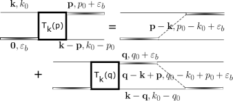
Figure 5: Diagrammatic representation of the three-body problem. The fermion-dimer scattering t-matrix is determined by repeating the fermion-exchange process infinitely-many times, forming eventually an integral equation.

By comparing the zero-loop, one-loop and two-loop approximations in Fig. 4, we observe that while the higher-loop contributions form a perturbative series in the $1/(m\alpha a_{s})<0$ region, they are of similar order in the $1/(m\alpha a_{s})>0$ region. Noting that $Z$ decays to $0$ in the $1/(m\alpha a_{s})\to-\infty$ limit, and that it increases as $\sqrt{|\varepsilon_{b}|}$ in the $1/(m\alpha a_{s})\to+\infty$ limit, this observation is caused by the incremental growth of the power of $Z$ that is coming from the additional dimer propagators within each loop. For this reason, a proper description of the latter region requires infinitely-many loop diagrams at all orders bedaque98 ; brodsky06 ; levinsen06 ; iskin08 ; iskin10 ; alzetto10 ; levinsen11 ; combescot17 . A practical way to handle such summations is presented in Fig. 5, where the fermion-dimer scattering t-matrix is determined by repeating the fermion-exchange process infinitely-many times, forming eventually an integral equation. In accordance with the Feynman rules, this diagram is given by

$$\mathcal{T}_{k}(p) =-\sigma_{y}G^{\mathrm{T}}(\mathbf{p}-\mathbf{k},p_{0}-k_{0}+\varepsilon_{b})\sigma_{y}$$

$$-\sum_{q}\mathcal{T}_{k}(q)D(\mathbf{q},q_{0}+\varepsilon_{b})G(\mathbf{k}-\mathbf{q},k_{0}-q_{0})$$

$$\times\sigma_{y}G^{\mathrm{T}}(\mathbf{q}-\mathbf{k}+\mathbf{p},q_{0}-k_{0}+p_{0}+\varepsilon_{b})\sigma_{y},$$ (21)

where the minus signs are due to the fermion exchanges. Integrating $q_{0}$ in the upper half plane where $\mathcal{T}_{k}(q)$ is analytic and there are two simple poles at $q_{0}=k_{0}-\varepsilon_{\mathbf{q}-\mathbf{k}}^{\pm}$, we reduce the t-matrix equation to

$$\mathcal{T}_{k}(\mathbf{p},p_{0})=-\frac{1}{2}\sum_{s}\frac{\sigma_{0}-s\widehat{\mathbf{k^{\prime}}}\cdot\boldsymbol{\sigma}}{p_{0}-k_{0}+\varepsilon_{b}-\varepsilon_{\mathbf{k^{\prime}}}^{s}}$$ (22)

$$-\frac{1}{4}\sum_{ss^{\prime}\mathbf{q}}\frac{D(\mathbf{q},k_{0}+\varepsilon_{b}-\varepsilon_{\mathbf{Q}}^{s})}{p_{0}+\varepsilon_{b}-\varepsilon_{\mathbf{Q}}^{s}-\varepsilon_{\mathbf{K}}^{s^{\prime}}}\mathcal{T}_{k}(\mathbf{q},k_{0}-\varepsilon_{\mathbf{Q}}^{s})$$

$$\times[(1-ss^{\prime}\widehat{\mathbf{Q}}\cdot\widehat{\mathbf{K}})\sigma_{0}+(s\widehat{\mathbf{Q}}-s^{\prime}\widehat{\mathbf{K}}-iss^{\prime}\widehat{\mathbf{Q}}\times\widehat{\mathbf{K}})\cdot\boldsymbol{\sigma}].$$

Here $\mathbf{k^{\prime}}=\mathbf{p}-\mathbf{k}$, $\mathbf{Q}=\mathbf{k}-\mathbf{q}$ and $\mathbf{K}=\mathbf{p}-\mathbf{k}+\mathbf{q}$ are introduced for the simplicity of the presentation.

In the usual three-body problem with no SOC, $t_{0}(\mathbf{p},p_{0})$ is not only a real function but it is also restricted to the so-called on-the-shell value $t_{0}[\mathbf{p},p_{0}=-p^{2}/(2m)]$ for both the incoming and outgoing fermions bedaque98 ; brodsky06 ; levinsen06 ; iskin08 ; iskin10 ; alzetto10 ; levinsen11 ; combescot17 . In addition, using the spherical symmetry of the t-matrix, the problem reduces to a simple integral equation with a single variable for $t_{0}(|\mathbf{p}|)$, whose numerical computation converges very fast. However, since the helicity bands are coupled due to the non-stationary dimers, there are two shells contributing to Eq. (22). Furthermore, given that the t-matrix is a $2\times 2$ matrix with complex elements, this reduces Eq. (22) to an eight coupled integral equations. Unfortunately, this is quite complicated, and the exact numerical solution of the three-body problem remains an open problem.

V Four-body problem

Motivated by the overall success of the Born approximation in the fermion-dimer scattering problem, here we apply the diagrammatic approach to the scattering t-matrix $t_{0}^{BB}(0)$ between two stationary dimers in the one-loop Born and two-loop approximations. Despite its simplicity, we expect $a_{BB}^{\mathrm{Born}}$ to be quite accurate in the $1/(m\alpha a_{s})\ll-1$ limit as the higher-order contributions form a perturbative series in the $1/(m\alpha a_{s})<0$ region. However, our results are only qualitative in the $1/(m\alpha a_{s})>0$ region, whose accurate description is beyond the scope of this paper brodsky06 ; levinsen06 ; alzetto13 .

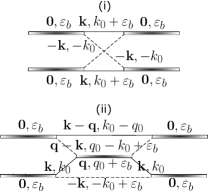
Figure 6: Diagrammatic representation of the (i) one-loop Born and (ii) two-loop contributions to the dimer-dimer scattering t-matrix.

The diagrammatic representation of the Born contribution to the dimer-dimer scattering t-matrix is shown in Fig. 6(i) pieri00 ; brodsky06 ; levinsen06 ; alzetto13 . In accordance with the Feynman rules, it is given by

$${t_{0}^{BB}}^{(1)}(0)=-\frac{\mathrm{Tr}}{2}\sum_{k}\big{[}\sigma_{y}G(\mathbf{k},k_{0}+\varepsilon_{b})\sigma_{y}G^{\mathrm{T}}(-\mathbf{k},-k_{0})\big{]}^{2},$$ (23)

where the minus sign is due to the fermion exchange. Noting the relations $(\sigma_{0}\pm\widehat{\mathbf{A}}\cdot\boldsymbol{\sigma})(\sigma_{0}\pm\widehat{\mathbf{A}}\cdot\boldsymbol{\sigma})=2(\sigma_{0}\pm\widehat{\mathbf{A}}\cdot\boldsymbol{\sigma}),$ and $(\sigma_{0}\pm\widehat{\mathbf{A}}\cdot\boldsymbol{\sigma})(\sigma_{0}\mp\widehat{\mathbf{A}}\cdot\boldsymbol{\sigma})=0,$ we first integrate $k_{0}$ in the upper half plane in which there are two double poles at $k_{0}=-\varepsilon_{\mathbf{k}}^{\pm}$, and reduce the t-matrix contribution to

$${t_{0}^{BB}}^{(1)}(0)=\frac{1}{2}\sum_{s\mathbf{k}}\frac{2}{(2\varepsilon_{\mathbf{k}}^{s}-\varepsilon_{b})^{3}}.$$ (24)

This is a physically intuitive result because, since all dimers are stationary in the Born diagram, the helicity bands are not coupled, and the diagram can be directly expressed as ${t_{0}^{BB}}^{(1)}(0)=(-1/2)\sum_{sk}\big{[}G_{s}(\mathbf{k},k_{0}+\varepsilon_{b})G_{s}(-\mathbf{k},-k_{0})\big{]}^{2}.$

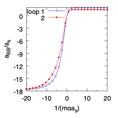
Figure 7: Dimer-dimer scattering length in the one-loop Born and two-loop approximations. The higher-loop contributions form a perturbative series in the $1/(m\alpha a_{s})<0$ region, but they are of similar order in the $1/(m\alpha a_{s})>0$ region.

In this paper, we are interested in the dimer-dimer scattering length $a_{BB}$ that is determined by pieri00 ; brodsky06 ; levinsen06 ; alzetto13

$$a_{BB}=\frac{m_{B}}{4\pi}Z^{2}t_{0}^{BB}(0).$$ (25)

Plugging ${t_{0}^{BB}}^{(1)}(0)=m\sqrt{m}(|\varepsilon_{b}|+2m\alpha^{2})/[16\pi(|\varepsilon_{b}|-m\alpha^{2})^{5/2}]$ above, we find he12b ; shenoy12a ; shenoy12b

$$a_{BB}^{\mathrm{Born}}=\frac{m_{B}(|\varepsilon_{b}|+2m\alpha^{2})\sqrt{|\varepsilon_{b}|-m\alpha^{2}}}{m\sqrt{m}|\varepsilon_{b}|^{2}},$$ (26)

in the Born approximation, which suggests that the dimer-dimer interaction is repulsive for all parameters. In Fig. 7, we show $a_{BB}^{\mathrm{Born}}$ as a function of $1/(m\alpha a_{s})$, which is analytically tractable in three limits: (i) $a_{BB}^{\mathrm{Born}}=-18a_{s}$ in the limit when $1/(m\alpha a_{s})\ll-1$, (ii) $a_{BB}^{\mathrm{Born}}=3\sqrt{2}/[m\alpha(2\sqrt{2}-1)]\approx 2.32/(m\alpha)$ in the unitarity limit when $1/(m\alpha a_{s})=0$, and (iii) $a_{BB}^{\mathrm{Born}}=2a_{s}$ in the limit when $1/(m\alpha a_{s})\gg 1$. Note that the latter limit recovers the usual four-body problem with no SOC in the $1/(m\alpha a_{s})\gg 1$ limit when $\alpha\to 0^{+}$.

To go beyond the Born approximation, we consider the two-loop contribution that is shown in Fig. 6(ii). In accordance with the Feynman rules, this diagram is given by

$${t_{0}^{BB}}^{(2)}(0)=-\frac{\mathrm{Tr}}{2}\sum_{kq}\sigma_{y}G^{\mathrm{T}}(\mathbf{q}-\mathbf{k},q_{0}-k_{0}+\varepsilon_{b})\sigma_{y}$$

$$G(\mathbf{k},k_{0})D(\mathbf{q},q_{0}+\varepsilon_{b})\sigma_{y}G^{\mathrm{T}}(-\mathbf{k},-k_{0}+\varepsilon_{b})\sigma_{y}G(\mathbf{k},k_{0})$$

$$\sigma_{y}G^{\mathrm{T}}(\mathbf{q}-\mathbf{k},q_{0}-k_{0}+\varepsilon_{b})\sigma_{y}G(\mathbf{k}-\mathbf{q},k_{0}-q_{0}).$$ (27)

We first integrate $q_{0}$ in the upper half plane in which there are two simple poles at $q_{0}=k_{0}-\varepsilon_{\mathbf{q}-\mathbf{k}}^{\pm}$, and then integrate $k_{0}$ in the upper half plane in which there are two simple poles at $k_{0}=\varepsilon_{b}-\varepsilon_{\mathbf{k}}^{\pm}$. This reduces the t-matrix contribution to

$${t_{0}^{BB}}^{(2)}(0)=\frac{1}{4}\sum_{ss^{\prime}\mathbf{k}\mathbf{q}}\frac{D(\mathbf{q},2\varepsilon_{b}-\varepsilon_{\mathbf{k}}^{s}-\varepsilon_{\mathbf{Q}}^{s^{\prime}})}{(2\varepsilon_{\mathbf{k}}^{s}-\varepsilon_{b})^{2}(2\varepsilon_{\mathbf{Q}}^{s^{\prime}}-\varepsilon_{b})^{2}}(1+ss^{\prime}\widehat{\mathbf{k}}\cdot\widehat{\mathbf{Q}}),$$ (28)

where $\mathbf{Q}=\mathbf{k}+\mathbf{q}$, and the remaining integrations are performed numerically in the $\mathbf{k}$ and $\mathbf{q}$ spaces integralnote . In Fig. 7, we show how the two-loop contribution affects $a_{BB}^{\mathrm{Born}}$ as a function of $1/(m\alpha a_{s})$. While the two-loop contribution is negligible in the $1/(m\alpha a_{s})\ll-1$ limit, it is comparable to $a_{BB}^{\mathrm{Born}}$ in the $1/(m\alpha a_{s})>0$ region.

VI Many-body problem

The fermion-dimer and dimer-dimer scattering lengths offer valuable insights for some of the many-body properties of Fermi gases. For instance, in the case of population-imbalanced Fermi gases, $a_{BF}$ and $a_{BB}$ can be used to map the strongly-interacting Fermi-Fermi mixture of $\uparrow$ and $\downarrow$ fermions to a weakly-interacting Bose-Fermi mixture of paired fermions (dimers) and unpaired (excess) ones pieri06 ; taylor07 ; iskin08 . In the parameter regime where this effective description holds, the existing literature on true Bose-Fermi mixtures can be easily utilized to characterize the imbalanced Fermi gases.

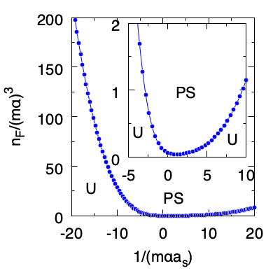
Figure 8: Critical boundary between the uniform superfluid (U) and phase separation (PS) that is determined by the effective weakly-interacting Bose-Fermi mixture description of a population-imbalanced Fermi gas in the Born approximation.

For instance, it is well-known that a weakly-interacting Bose-Fermi mixture is unstable against phase separation with a negative compressibility when the density of fermions $n_{F}$ satisfies iskin11 $n_{F}\geq 4\pi^{4}U_{BB}^{3}/(3m_{F}^{3}U_{BF}^{6})$ in three dimensions, where $U_{BB}=4\pi a_{BB}/m_{B}$ is the repulsive interaction between bosons, and $U_{BF}=4\pi a_{BF}/m_{BF}$ is the repulsive interaction between fermions and bosons. Thus, the Bose-Fermi mixture phase separates when

$$n_{F}\geq\frac{4\pi}{3}\frac{m^{3}m_{B}^{3}}{(m_{B}+m)^{6}}\frac{a_{BB}^{3}}{a_{BF}^{6}},$$ (29)

and is otherwise uniform. By plugging the Born approximations Eqs. (16) and (26) into Eq. (29), we obtain the corresponding relation for the stability of a population-imbalanced Fermi gas with SOC. The critical boundary between the uniform superfluid and phase separation is shown in Fig. 8.

Here we remark in passing that one can study BCS-BEC evolution for any given $a_{s}$ by tuning the strength $\alpha$ of the SOC, no matter how small or large the value of $a_{s}$ is and independently of its sign. Its physical mechanism is the SOC-induced enhancement of $\varepsilon_{b}$ through the increase of the single particle density of states. In particular, when $\alpha$ is large, the nature of the bosons that make up the BEC is determined solely by $\alpha a_{s}$. For this reason, these bosons are sometimes called rashbons in the recent literature since their properties are determined by SOC alone. See Refs. zhai11 ; iskin11 ; hu11 ; he12a ; he12b ; shenoy12a ; shenoy12b for further discussion, including the effective Gross-Pitaevskii description of the weakly-interacting dimers in the BEC limit.

VII Anisotropic (Rashba) spin-orbit coupling

Our results can be easily generalized to anisotropic SOC fields. For instance, in the presence of a Rashba SOC, the one-body Hamiltonian is governed by $h_{\mathbf{k}}=\varepsilon_{\mathbf{k}}\sigma_{0}+\alpha\mathbf{k_{\perp}}\cdot\boldsymbol{\sigma},$ where $\mathbf{k}=(\mathbf{k_{\perp}},k_{z})$ and $\mathbf{k_{\perp}}=(k_{x},k_{y})$, leading to $\varepsilon_{\mathbf{k}}^{s}=(k_{\perp}^{2}+k_{z}^{2})/(2m)+s\alpha k_{\perp}.$ Therefore, the ground state of the $-$-helicity band corresponds to a degenerate ring of $\mathbf{k_{\perp}}$ states with the radius $k_{m}=m\alpha$ at $k_{z}=0$ and energy $\varepsilon_{\mathbf{k}_{m}}^{-}=-m\alpha^{2}/2$.

In the lowest order in $\mathbf{q}=(\mathbf{q_{\perp}},q_{z})$ and $q_{0}$, Eq. (6) has the generic structure of a simple pole iskin11 ; hu11 ; he12a ; he12b ; shenoy12a ; shenoy12b

$$D(\mathbf{q},q_{0})=\frac{Z}{q_{0}-q_{\perp}^{2}/(2m_{B,\perp})-q_{z}^{2}/(2m_{B,z})+\mu_{B}+i0^{+}}$$ (30)

where $Z=8\pi(|\varepsilon_{b}|-m\alpha^{2})/(m\sqrt{m|\varepsilon_{b}|})$ corresponds to the residue of the pole, $2m/m_{B,\perp}=(2|\varepsilon_{b}|-m\alpha^{2})/(2|\varepsilon_{b}|)-[(|\varepsilon_{b}|-m\alpha^{2})/(2|\varepsilon_{b}|)]\log(1-m\alpha^{2}/|\varepsilon_{b}|)$ and $m_{B,z}=2m$ determine the anisotropic effective mass of the dimer. In addition, $\mu_{B}=|\varepsilon_{b}|$ is determined by $1/(m\alpha a_{s})=\sqrt{|\varepsilon_{b}|/(m\alpha^{2})}-\log[\sqrt{|\varepsilon_{b}|/(|\varepsilon_{b}|-m\alpha^{2})}+\sqrt{m\alpha^{2}/(|\varepsilon_{b}|-m\alpha^{2})}].$ This expression is analytically tractable in three limits zhai11 ; iskin11 ; hu11 : we find that (i) $\varepsilon_{b}=-m\alpha^{2}-4m\alpha^{2}e^{2/(m\alpha a_{s})-2}$ and $m_{B,\perp}=4m$ in the limit when $1/(m\alpha a_{s})\ll-1$, (ii) $\varepsilon_{b}\approx-1.44m\alpha^{2}$ and $m_{B,\perp}\approx 2.40m$ in the unitarity limit when $1/(m\alpha a_{s})=0$, and (iii) $\varepsilon_{b}=-1/(ma_{s}^{2})$ and $m_{B,\perp}=2m$ in the limit when $1/(m\alpha a_{s})\gg 1$. Note that the latter limit recovers the usual two-body problem with no SOC in the $1/(m\alpha a_{s})\gg 1$ limit when $\alpha\to 0^{+}$.

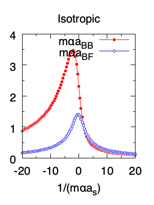
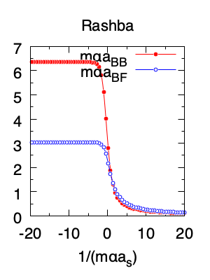
Figure 9: Dimer-dimer (red) and fermion-dimer (blue) scattering lengths for the isotropic SOC (left: same as in Fig. 4) versus Rashba SOC (right) in the Born approximations.

Since $k=(m\alpha\widehat{\mathbf{k_{\perp}}},-m\alpha^{2}/2)$ corresponds to the lowest-energy eigenstate in the $-$-helicity band, Eq. (15) gives ${t_{k}^{--}}^{(0)}(0)=1/(|\varepsilon_{b}|-m\alpha^{2}).$ By plugging it into Eq. (13), we find

$$a_{BF}^{\mathrm{Born}}=\frac{2m_{BF}}{m\sqrt{m|\varepsilon_{b}|}}$$ (31)

in the Born approximation, where $m_{B}$ refers to the geometric mean $(m_{B,\perp}^{2}m_{B,z})^{1/3}$ of the anisotropic effective mass shenoy12b . In Fig. 9, we show $a_{BF}^{\mathrm{Born}}$ as a function of $1/(m\alpha a_{s})$, which is analytically tractable in three limits: (i) $a_{BF}^{\mathrm{Born}}\approx 3.04/(m\alpha)$ in the limit when $1/(m\alpha a_{s})\ll-1$, (ii) $a_{BF}^{\mathrm{Born}}\approx 2.31/(m\alpha)$ in the unitarity limit when $1/(m\alpha a_{s})=0$, and (iii) $a_{BF}^{\mathrm{Born}}=8a_{s}/3$ in the limit when $1/(m\alpha a_{s})\gg 1$. Note again the latter limit recovers the usual three-body problem with no SOC in the $1/(m\alpha a_{s})\gg 1$ limit when $\alpha\to 0^{+}$.

Similarly, Eq. (24) gives ${t_{0}^{BB}}^{(1)}(0)=m\sqrt{m}(|\varepsilon_{b}|+m\alpha^{2})/[16\pi(|\varepsilon_{b}|-m\alpha^{2})^{2}\sqrt{|\varepsilon_{b}|}],$ and by plugging it in Eq. (25), we find

$$a_{BB}^{\mathrm{Born}}=\frac{m_{B}(|\varepsilon_{b}|+m\alpha^{2})}{m\sqrt{m}\sqrt{|\varepsilon_{b}|}^{3}},$$ (32)

in the Born approximation. In Fig. 9, we show $a_{BB}^{\mathrm{Born}}$ as a function of $1/(m\alpha a_{s})$, which is analytically tractable in three limits: (i) $a_{BB}^{\mathrm{Born}}\approx 6.35/(m\alpha)$ in the limit when $1/(m\alpha a_{s})\ll-1$, (ii) $a_{BB}^{\mathrm{Born}}\approx 3.19/(m\alpha)$ in the unitarity limit when $1/(m\alpha a_{s})=0$, and (iii) $a_{BB}^{\mathrm{Born}}=2a_{s}$ in the limit when $1/(m\alpha a_{s})\gg 1$. Note again that the latter limit recovers the usual four-body problem with no SOC in the $1/(m\alpha a_{s})\gg 1$ limit when $\alpha\to 0^{+}$.

In contrast to the isotropic SOC case where $a_{BF}$ and $a_{BB}$ are non-monotonous functions of $1/(m\alpha a_{s})$, they evolve monotonously in the Rashba SOC. Their saturations in the $1/(m\alpha a_{s})\ll-1$ limit are caused by the exact cancellation of the decay of $Z$ with the divergence of the t-matrices. The decay is faster in the isotropic case, causing the peak in the intermediate region. Despite this major difference, the isotropic and Rashba SOC cases share some common properties. For instance, the decrease, increase and saturation of $a_{BF}$ are in full coordination with those of $a_{BB}$. In addition, we note that $a_{BF}$ is greater (smaller) than $a_{BB}$ in approximately the $1/(m\alpha a_{s})\gtrless 0$ regions.

VIII Conclusion

In summary, we studied how SOC affects the fermion-dimer and dimer-dimer scattering lengths in the Born approximation, and benchmarked their accuracy with the higher-order approximations. We considered both isotropic and Rashba couplings in three dimensions, and found that the Born approximation gives accurate results for both $a_{BF}$ and $a_{BB}$ in the $1/(m\alpha a_{s})\ll-1$ limit. This is because while the higher-loop contributions form a perturbative series in the $1/(m\alpha a_{s})<0$ region, they are of similar order in the $1/(m\alpha a_{s})>0$ region. We found that the perturbations are controlled by the residue $Z$ of the dimer propagator, which decays to $0$ in the $1/(m\alpha a_{s})\to-\infty$ limit, and increases as $\sqrt{|\varepsilon_{b}|}$ in the $1/(m\alpha a_{s})>0$ region. Therefore, it may be sufficient to consider a finite number of higher-order loop diagrams in the $1/(m\alpha a_{s})<0$ region.

On the other hand, a proper description of the $1/(m\alpha a_{s})>0$ region requires infinitely-many loop diagrams at all orders. In the case of three-body problem, we derived a coupled set of integral equations for the exact atom-dimer scattering length, but its numerical solutions remain an open problem. It may be possible to solve the exact three-body problem through partial-wave expansion, and address the possibility of a three-body bound state in this system. In addition, one may also study the importance of the full momentum and/or full frequency dependences of the dimer propagator in the three- and/or four-body problems.

Appendix A Binding energy and effective mass of the dimer

For the sake of completeness, we present the binding energy $|\varepsilon_{b}|-m\alpha^{2}$ and effective mass $m_{B}$ of the dimer in Fig. 10, where 3D SOC field refers to $\alpha\mathbf{k}$ with $\mathbf{k}=(k_{x},k_{y},k_{z})$, 2D one to $\alpha\mathbf{k_{\perp}}$ with $\mathbf{k_{\perp}}=(k_{x},k_{y},0)$, and 1D one to $\mathbf{k}=(k_{x},0,0)$. The latter case is trivial because as the 1D SOC field can be gauged away from the $\mathbf{k}$-space integrations, it is equivalent to the usual two-body problem with no SOC iskin11 . Therefore, a two-body bound state exists only when $a_{s}>0$ with an effective mass $m_{B}=2m$ that is isotropic in space.

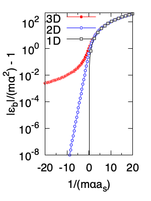
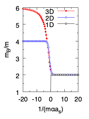
Figure 10: Binding energy $|\varepsilon_{b}|-m\alpha^{2}$ and effective mass $m_{B,x}$ of the dimer. Here, 3D SOC field is shown in red and refers to $\alpha\mathbf{k}$ with $\mathbf{k}=(k_{x},k_{y},k_{z})$, 2D one is shown in blue and refers to $\alpha\mathbf{k_{\perp}}$ with $\mathbf{k_{\perp}}=(k_{x},k_{y},0)$, and 1D one is shown in black and refers to $\mathbf{k}=(k_{x},0,0)$.

In contrast to the 1D case, a two-body bound state exists for all $a_{s}$ in both 3D (isotropic) and 2D (Rashba) SOC fields, which is caused by the increase in the low-energy density of one-body states zhai11 ; iskin11 ; hu11 ; he12a ; he12b ; shenoy12a ; shenoy12b . In addition, while the effective mass of the dimer is isotropic in the 3D case where $m_{B}=m_{B,x}=m_{B,y}=m_{B,z}$ is shown in the figure, it is anisotropic in the 2D case where only $m_{B,\perp}=m_{B,x}=m_{B,y}$ is shown in the figure, and $m_{B,z}=2m$ for all $a_{s}$.

References

- (1) P. F. Bedaque and U. van Kolck, Nucleon-deuteron scattering from an effective field theory, Physics Letters B 428, 221 (1998).
- (2) I. V. Brodsky, M. Yu. Kagan, A. V. Klaptsov, R. Combescot, and X. Leyronas, Exact diagrammatic approach for dimer-dimer scattering and bound states of three and four resonantly interacting particles, JETP Lett. 82, 273 (2005); Phys. Rev. A 73, 032724 (2006).
- (3) J. Levinsen and V. Gurarie, Properties of strongly paired fermionic condensates, Phys. Rev. A 73, 053607 (2006).
- (4) M. Iskin and C. A. R. Sá de Melo, Fermi-Fermi mixtures in the strong-attraction limit, Phys. Rev. A 77, 013625 (2008).
- (5) M. Iskin Dimer-atom scattering between two identical fermions and a third particle, Phys. Rev. A 81, 043634 (2010).
- (6) F. Alzetto, R. Combescot, and X. Leyronas, Atom-dimer scattering length for fermions with different masses: Analytical study of limiting cases, Phys. Rev. A 82, 062706 (2010).
- (7) J. Levinsen and D. S. Petrov, Atom-dimer and dimer-dimer scattering in fermionic mixtures near a narrow Feshbach resonance, Eur. Phys. J. D 65, 67 (2011).
- (8) P. Pieri and G. C. Strinati, Strong-coupling limit in the evolution from BCS superconductivity to Bose-Einstein condensation, Phys. Rev. B 61, 15370 (2000).
- (9) F. Alzetto, R. Combescot, and X. Leyronas, Dimer-dimer scattering length for fermions with different masses: analytical study for large mass ratio, Phys. Rev. A 87, 022704 (2013).
- (10) G. V. Skorniakov and K. A. Ter-Martirosian, Three Body Problem for Short Range Forces. I. Scattering of Low Energy Neutrons by Deuterons, Zh. Eksp. Teor. Fiz. 31, 775 (1956); and Sov. Phys. JETP 4, 648 (1957).
- (11) D. S. Petrov, Three-body problem in Fermi gases with short-range interparticle interaction, Phys. Rev. A 67, 010703(R) (2003).
- (12) D. S. Petrov, C. Salomon, and G. V. Shlyapnikov, Diatomic molecules in ultracold Fermi gases - Novel composite bosons, J. Phys. B: At. Mol. Opt. Phys. 38, S645 (2005).
- (13) R. Combescot, Three-Body Coulomb Problem, Phys. Rev. X 7, 041035 (2017).
- (14) For example, see one of the most recent reviews by G. C. Strinati, P. Pieri, G. Roepke, P. Schuck, and M. Urban, The BCS-BEC crossover: From ultra-cold Fermi gases to nuclear systems Phys. Rep. 738, 1 (2018).
- (15) P. Pieri and G. C. Strinati Trapped Fermions with Density Imbalance in the Bose-Einstein Condensate Limit, Phys. Rev. Lett. 96, 150404 (2006).
- (16) E. Taylor, A. Griffin, and Y. Ohashi, Spin-polarized Fermi superfluids as Bose-Fermi mixtures, Phys. Rev. A 76, 023614 (2007).
- (17) L. W. Cheuk, A. T. Sommer, Z. Hadzibabic, T. Yefsah, W. S. Bakr, and M. W. Zwierlein, Spin-Injection Spectroscopy of a Spin-Orbit Coupled Fermi Gas, Phys. Rev. Lett. 109, 095302 (2012).
- (18) R. A. Williams, M. C. Beeler, L. J. LeBlanc, K. Jiménez-García, and I. B. Spielman, Raman-induced interactions in a single-component Fermi gas near an s-wave Feshbach resonance, Phys. Rev. Lett. 111, 095301 (2013).
- (19) L. Huang, Z. Meng, P. Wang, P. Peng, S.-L. Zhang, L. Chen, D. Li, Q. Zhou, and J. Zhang, Experimental realization of a two-dimensional synthetic spin-orbit coupling in ultracold Fermi gases, Nat. Phys. 12, 540 (2016).
- (20) Z. Meng, L. Huang, P. Peng, D. Li, L. Chen, Y. Xu, C. Zhang, P. Wang, and J. Zhang, Experimental Observation of a Topological Band Gap Opening in Ultracold Fermi Gases with Two-Dimensional Spin-Orbit Coupling, Phys. Rev. Lett. 117, 235304 (2016).
- (21) Z.-Q. Yu and H. Zhai, Spin-Orbit Coupled Fermi Gases across a Feshbach Resonance, Phys. Rev. Lett. 107, 195305 (2011).
- (22) M. Iskin and A. L. Subaşı, Quantum phases of atomic Fermi gases with anisotropic spin-orbit coupling, Phys. Rev. A 84, 043621 (2011).
- (23) H. Hu, L. Jiang, X.-J. Liu, and H. Pu, Probing Anisotropic Superfluidity in Atomic Fermi Gases with Rashba Spin-Orbit Coupling, Phys. Rev. Lett. 107, 195304 (2011).
- (24) L. He and X.-G. Huang, BCS-BEC Crossover in 2D Fermi Gases with Rashba Spin-Orbit Coupling, Phys. Rev. Lett. 108, 145302 (2012).
- (25) L. He and X.-G. Huang, BCS-BEC crossover in three-dimensional Fermi gases with spherical spin-orbit coupling, Phys. Rev. B 86, 014511 (2012).
- (26) J. P. Vyasanakere and V. B. Shenoy, Rashbons: properties and their significance, New J. of Phys. 14, 043041 (2012).
- (27) J. P. Vyasanakere and V. B. Shenoy, Collective excitations, emergent Galilean invariance, and boson-boson interactions across the BCS-BEC crossover induced by a synthetic Rashba spin-orbit coupling, Phys. Rev. A 86, 053617 (2012).
- (28) To achieve a reliable numerical convergence, we change the limits of the radial integration from to via the change of variables , i.e.,