An HST Survey of Protostellar Outflow Cavities: Does Feedback Clear Envelopes?

Nolan M. Habel¹¹affiliation: Ritter Astrophysical Research Center, Department of Physics and Astronomy, University of Toledo, 2801 W. Bancroft Street, Toledo, OH 43606, USA , S. Thomas Megeath¹¹affiliation: Ritter Astrophysical Research Center, Department of Physics and Astronomy, University of Toledo, 2801 W. Bancroft Street, Toledo, OH 43606, USA , Joseph Jon Booker¹¹affiliation: Ritter Astrophysical Research Center, Department of Physics and Astronomy, University of Toledo, 2801 W. Bancroft Street, Toledo, OH 43606, USA , William J. Fischer²²affiliation: Space Telescope Science Institute, 3700 San Martin Drive, Baltimore, MD 21218, USA , Marina Kounkel³³affiliation: Department of Physics and Astronomy, Western Washington University, 516 High st., Bellingham, WA, 98225 , Charles Poteet¹¹affiliation: Ritter Astrophysical Research Center, Department of Physics and Astronomy, University of Toledo, 2801 W. Bancroft Street, Toledo, OH 43606, USA ²²affiliation: Space Telescope Science Institute, 3700 San Martin Drive, Baltimore, MD 21218, USA , Elise Furlan⁴⁴affiliation: NASA Exoplanet Science Institute, Caltech/IPAC, Mail Code 100-22, 1200 E. California Blvd., Pasadena, CA 91125, USA , Amelia Stutz⁵⁵affiliation: Max-Planck-Institut für Astronomie, Königstuhl 17, D-69117 Heidelberg, Germany ⁶⁶affiliation: Departmento de Astronomía, Facultad Ciencias Físicas y Matemáticas, Universidad de Concepción, Av. Esteban Iturra s/n Barro Universitario, Casilla 160-C, Concepción, Chile , P. Manoj⁷⁷affiliation: Department of Astronomy and Astrophysics, Tata Institute of Fundamental Research, Homi Bhabha Road, Colaba, Mumbai 400005, India , John J. Tobin⁸⁸affiliation: National Radio Astronomy Observatory, 520 Edgemont Rd., Charlottesville,VA 22903, USA , Zsofia Nagy¹¹affiliation: Ritter Astrophysical Research Center, Department of Physics and Astronomy, University of Toledo, 2801 W. Bancroft Street, Toledo, OH 43606, USA ⁹⁹affiliation: Konkoly Observatory, Research Centre for Astronomy and Earth Sciences, H-1121 Budapest, Konkoly Thege út 15–17, Hungary , Riwaj Pokhrel¹¹affiliation: Ritter Astrophysical Research Center, Department of Physics and Astronomy, University of Toledo, 2801 W. Bancroft Street, Toledo, OH 43606, USA , Dan Watson¹⁰¹⁰affiliation: Department of Physics and Astronomy, University of Rochester, Rochester, NY 14627, USA

Abstract

We study protostellar envelope and outflow evolution using Hubble Space Telescope NICMOS or WFC3 images of 304 protostars in the Orion Molecular clouds. These near-IR images resolve structures in the envelopes delineated by the scattered light of the central protostars with 80 AU resolution and they complement the $1.2870\text{\,}\mathrm{\SIUnitSymbolMicro m}$ spectral energy distributions obtained with the Herschel Orion Protostar Survey program (HOPS). Based on their $1.60\text{\,}\mathrm{\SIUnitSymbolMicro m}$ morphologies, we classify the protostars into five categories: non-detections, point sources without nebulosity, bipolar cavity sources, unipolar cavity sources, and irregulars. We find point sources without associated nebulosity are the most numerous, and show through monochromatic Monte Carlo radiative transfer modeling that this morphology occurs when protostars are observed at low inclinations or have low envelope densities. We also find that the morphology is correlated with the SED-determined evolutionary class with Class 0 protostars more likely to be non-detections, Class I protostars to show cavities and flat-spectrum protostars to be point sources. Using an edge detection algorithm to trace the projected edges of the cavities, we fit power-laws to the resulting cavity shapes, thereby measuring the cavity half-opening angles and power-law exponents. We find no evidence for the growth of outflow cavities as protostars evolve through the Class I protostar phase, in contradiction with previous studies of smaller samples. We conclude that the decline of mass infall with time cannot be explained by the progressive clearing of envelopes by growing outflow cavities. Furthermore, the low star formation efficiency inferred for molecular cores cannot be explained by envelope clearing alone.

^†^†software: Astropy (The Astropy Collaboration et al., 2013), DrizzlePac (STSCI Development Team, 2012), HO-CHUNK (Whitney & Hartmann, 1992, 1993),Matplotlib (Hunter, 2007), NumPy (Walt et al., 2011), SciPy (Oliphant, 2007), Tiny Tim (Krist et al., 2011)

\savesymbol

tablenum \restoresymbolSIXtablenum

1 Introduction

Low mass protostars are characterized by a rapid evolution, with the accretion of the stellar mass, the formation of disks and potentially the initiation of planet formation occurring within $0.5\text{\,}\mathrm{Myr}$ (Arce & Sargent, 2006, Cassen & Moosman, 1981, Dunham et al., 2014, ALMA Partnership et al., 2015, Dipierro et al., 2015). The defining characteristic of the protostellar phase is the presence of a dusty, infalling envelope which absorbs and reprocesses most of the luminosity from the central protostar. In the initial phases of protostellar evolution, the envelope dominates the mass, while in the later phases, most of the mass is already accreted onto the star. Even in these later phases, the mass of the envelope typically exceeds that of the circumstellar disks surrounding the central protostar (e.g. Fischer et al., 2014); hence, infall in these phases shapes the properties of circumstellar disks and sets the stage for planet formation. Understanding the factors that govern the evolution of the envelopes, and thereby influence mass accretion and the properties of nascent disks, is a key problem in star and planet formation studies.

This evolution is accompanied by a rapid change in the shape of the SEDs produced by the reprocessing and scattering of radiative energy in the evolving disks and envelopes (Furlan et al., 2016). Since the central protostar is deeply embedded in its envelope, the effective temperatures and photospheric luminosities of protostars typically cannot be measured directly. In most cases, unlike pre-main sequence stars, they cannot be reliably placed on HR diagrams and compared to evolutionary tracks to estimate masses and ages. Instead, the evolution of protostars is largely inferred from the shape of their SEDs. This evolution is typically measured by sorting protostars into bulk evolutionary classes based on the percentage of luminosity radiated in the sub-millimeter, their near- to mid-infrared spectral index or $T_{\text{bol}}$ , the bolometeric temperature (e.g., Adams & Shu, 1985, Myers & Ladd, 1993, Andre et al., 1993, Stutz et al., 2013, Dunham et al., 2014, Furlan et al., 2016). The observed sequence of evolutionary classes, Class 0, Class I and flat-spectrum, shows the peak of the SED shifting from the far-infrared to the mid-infrared and the SED flattening as the protostars evolve and the envelopes dissipate (e.g., Furlan et al., 2016). Class II objects can be identified by their decreasing near- to mid-IR SED slopes and are primarily pre-main sequence stars with disks that have exited the protostellar phase.

Due to the flattening of envelopes by rotation and the clearing of cavities in the envelopes by outflows, the luminosity of the protostars is not radiated isotropically, but is preferentially beamed along the rotation axis of the protostars. The resulting SEDs depend on the inclination of the protostars, and the effects of inclination on the SEDs are difficult to disentangle from those due to evolution (Kenyon et al., 1993, Whitney et al., 2003). To circumvent this degeneracy, Whitney & Hartmann (1993) and Robitaille et al. (2007) proposed a set of evolutionary stages which are dependent on the physical properties of the envelopes and not inclination; however, it is often difficult to reliably infer the stage of a protostar from the obseved SED alone. Nevertheless, taking into account the uncertainties due to inclination, Furlan et al. (2016) demonstrate that the observed SEDs of the distinct evolutionary classes require the dissipation of the envelope, with the density of the envelope gas (as inferred by model fits to the SEDs) dropping by a factor of 50 between the Class 0 and flat-spectrum phases. This shows that the envelopes decrease in density dramatically during the Class I phase.

Although SEDs are currently the primary information we have on large samples of protostars, imaging at millimeter, submillimeter and near-infrared wavelengths can be used to study protostellar evolution by resolving structures in the envelope that may change as protostars evolve (e.g., Arce & Sargent, 2006). HST near-infrared images of protostars resolve structures seen directly in light scattered by dust grains in an envelope or in silhouette against scattered light, placing constraints on the envelopes and disks that are complementary to those inferred from SEDs. HST imaging of protostars by Padgett et al. (1999), Allen et al. (2002), Terebey et al. (2006) and Fischer et al. (2014) show outflow cavities illuminated in scattered light, edge-on disks seen in absorption and shadows cast into the envelopes by flared disks.

Of particular interest is the role of feedback from outflows in driving the evolution of protostars by clearing the envelope and halting infall. SED-based measurements cannot reliably constrain outflow cavity sizes (Furlan et al., 2016); hence, studies of the growth of outflow cavities must rely on observations that spatially resolve structures in envelopes. The \ceCO observations of nine Class 0, I and II sources by Arce & Sargent (2006) showed a widening in outflow size with evolutionary class. Bolstering their sample by nine sources in the literature, they found evidence that outflow cavity sizes increase progressively as protostars evolve. Tobin et al. (2007)Seale & Looney (2008) used Spitzer IRAC images of protostar outflow cavities illuminated in scattered light to study the growth of cavities, and the latter authors found some evidence of outflow cavity growth with evolution, with significant scatter.

These studies suggest that feedback from outflows play a significant role in the decrease or halting of infall and accretion. Although accretion from the disk can continue after infall stops, the resulting increase in mass is small compared to the stellar mass. By reducing or halting infall, feedback can also play an important role in the star formation efficiency inferred from the core mass function. In particular, the mass function of cores identified in sub-mm measurements can reproduce the initial mass function if each core forms a star with a star formation efficiency (defined by the stellar to initial core mass) of $3040\text{\,}\mathrm{\char 37\relax}$ (Alves et al., 2007, Könyves et al., 2015). Furthermore, simulations of protostars including feedback can produce star formation efficiencies of $50\text{\,}\mathrm{\char 37\relax}$ or lower (Machida & Hosokawa, 2013, Machida & Matsumoto, 2012, Hansen et al., 2012, Offner & Arce, 2014, Offner & Chaban, 2017).

There are difficulties, however, in explaining the low star formation efficiency with feedback alone. Single dish radio observations suggest that outflows may carry too little mass to clear out the envelope in $0.5\text{\,}\mathrm{Myr}$ (Hatchell et al., 2007, Curtis et al., 2010). Furthermore, even large cavities clear less than half of the envelope mass (Frank et al., 2014). These studies, however, likely underestimate the amount of entrained, low-velocity gas in the outflow (Dunham et al., 2014). ALMA observations can now map these lower-velocity flows and show whether they transport a significant fraction of the envelope gas over the lifetime of the protostar (Zhang et al., 2016).

To further investigate the impact of outflows on protostellar envelopes, we use in this work the largest HST survey of protostars to date. This survey focuses on the sample of protostars targeted by the Herschel Orion Protostar Survey, or HOPS. The protostars were identified using combined 2MASS and Spitzer photometry from the Spitzer Orion Survey (Megeath et al., 2012, 2016) and observed with Herschel and APEX to obtain well sampled $1.2870\text{\,}\mathrm{\SIUnitSymbolMicro m}$ SEDs. This sample was supplemented by very red protostars discovered with Herschel (Stutz et al., 2013, Tobin et al., 2016). Furlan et al. (2016) published the SEDs of the entire sample and then presented model fits to 319 of the protostars and eleven pre-main sequence stars after rejecting likely extragalactic contamination and sources without Herschel detections. The HST survey examined 304 of these sources, (enumerated in Table 4), using initially NICMOS at 1.60 and $2.05\text{\,}\mathrm{\SIUnitSymbolMicro m}$ , and then after the failure of NICMOS, WFC3 at $1.60\text{\,}\mathrm{\SIUnitSymbolMicro m}$ . A search for binary systems using these data was published by Kounkel et al. (2016).

The morphologies of outflow cavities carved by the outflows can be seen by mapping the location of the cavity wall in scattered light. The volumes of the cavities carved by outflows can then be directly measured. The mechanism for creating these cavities, whether by jet precession, wide-angled winds or jet entrainment (Raga & Cabrit, 1993, Lee et al., 2001, Matzner & McKee, 1999, Ybarra et al., 2006), is still debated. Independent of the underlying mechanism, the scattered-light cavities provide a direct measurement of the cleared gas with the $80\text{\,}\mathrm{AU}$ ( $0.18\text{\,}\mathrm{\SIUnitSymbolArcsecond}$ ) resolution of HST. These are used in this work to estimate the fraction of the volume cleared, which provides an estimate of the fraction of mass cleared.

In Section 2, we discuss the observations used in this paper. We make use of radiative transfer modeling, described in Section 3, to understand the morphologies of the observed cavities and to calibrate the relationship between the scattered-light distributions and the cavity properties. In Section 4, we present the morphologies of the observed protostar and our analysis of the cavity sizes. Finally, we discuss the implications for protostellar evolution in Section 5. Images of the protostars in our sample are shown in Appendix A.

2 HST Observations of The Sample

The Hubble Space Telescope observations were assembled from two GO programs and a snapshot program. The bulk of the sample was observed in program GO 11548. The Near Infrared Camera and Multi-Object Spectrometer’s (NICMOS) F205W and F160W filters were used for a total of 87 orbits in August and September of 2008 to image 92 objects in the HOPS catalog, before the failure of the cryocooler of NICMOS. After the June 2009 deployment of the Wide Field Camera 3 (WFC3), 126 orbits were used between August 2009 and December 2010 to observe 237 HOPS objects with the F160W filter. The observation and reduction of these data is described in Kounkel et al. (2016). A subsequent program using WFC3, SNAP 14181, was designed to target multiple star forming regions within 500 pc. It completed observations during 114 orbits between December 2015 and September 2017, 10 of which imaged 13 objects in the Orion Molecular Clouds. A final WFC3 study, program GO 14695, targeted four objects in Orion with weak 24 $\mu$ m fluxes atypical of protostars. These observations were conducted in September 2016 with four orbits. For these final two programs we used the standard data products produced from the calwf3 data reduction pipeline which were then combined with AstroDrizzle from the DrizzlePac package using a drop size of 1 onto a pixel scale of $0.13\text{\,}\mathrm{\SIUnitSymbolArcsecond}$ .

The NICMOS observations used the NIC2 camera, which has a $0.075\text{\,}\mathrm{\SIUnitSymbolArcsecond}$ pixel size and resolution of $0.15\text{\,}\mathrm{\SIUnitSymbolArcsecond}$ . Integration times were $1215.4\text{\,}\mathrm{s}$ and $767.6\text{\,}\mathrm{s}$ for F160W and F205W filters, respectively. The WFC3 integration times were $2496.2\text{\,}\mathrm{s}$ for GO 11548, $1596.9\text{\,}\mathrm{s}$ for SNAP 14181, and $2396.9\text{\,}\mathrm{s}$ for GO 14695. All have a $0.18\text{\,}\mathrm{\SIUnitSymbolArcsecond}$ angular resolution and a pixel size of $0.13\text{\,}\mathrm{\SIUnitSymbolArcsecond}$ . In this work we adopt a distance to Orion of 420 parsecs for consistency with Furlan et al. (2016). This is within the range of distances found in Kounkel et al. (2018) and Großschedl et al. (2018) through APOGEE and Gaia measurements. At this distance, both NICMOS and WFC3 resolve structures down to $80\text{\,}\mathrm{AU}$ scales.

Nine images taken with NICMOS are excluded from this analysis due to the lack of guide star tracking; these contain HOPS 46, 47, 134, 139, 149, 227, 250, 271 and 276. Three WFC3 images, containing HOPS 293, 330 and 336, were also excluded due to what appear to be tracking failures. One additional WFC3 observation was excluded due to an apparent pointing error with its target object, HOPS 100, only partially appearing on the edge of the frame. Three images where only one guide star was used, those containing HOPS 10, 177, 316 and 358, may suffer from a small amount of rotation during the exposure, although this is not apparent in the data. These are included in our program. Twenty-seven of the HOPS targets were imaged by both NICMOS and WFC3 due to their proximity to other protostars. Of these sources, only HOPS 250 showed a clear difference between the two observations due to the tracking failure.

Some of the HOPS targets were classified as potential extragalactic contamination by Furlan et al. (2016) based on the presence of PAH features in their Spitzer IRS spectrum, lack of silicate absorption at $10\text{\,}\mathrm{\SIUnitSymbolMicro m}$ , or the shape of the mid-infrared continuum (see appendix of Furlan et al., 2016). The HST observations provide an independent means for separating galaxies from protostars. Only one source, HOPS 339, is conclusively determined by its morphology to be a galaxy and is omitted from the table in the appendix of this work (Table 4). The WFC3 image of this source is shown in Appendix E. Conversely, we add back into our sample and assign a class to HOPS 48, 67, and 301. These have morphologies in WFC3 imaging indicative of protostellar cavities. The nature of the remaining potentially extragalactic sources could not be clarified through WFC3 imaging. In program GO 14695, two of the four targeted sources were found not to be protostars; one was a galaxy and one an outflow knot; neither of these has a HOPS number (see Appendix E). In total, we imaged 304 objects in our sample. We note that 7 of these were determined to be Class II objects by their SEDs in Furlan et al. (2016). Since these sources are in the HOPS sample and may have residual envelopes, we keep them in the analysis. We typically use “protostars” to refer to this entire sample. In addition, we serendipitously observed two Class II sources with nebulosity in our images (Kounkel et al., 2016). We describe these objects in Appendix D.

Refer to caption — Figure 1: The definition of the cavity half-opening angle used in this paper and in the HO-CHUNK code. The circular region is the outer radius of the envelope of the protostar in these models, set to 8000 AU; the parabolic ( $n=2$ ) black line is the adopted boundary of the evacuated outflow cavity. The central protostar is located at the origin. The cavity half-opening angle is defined by the angle between the dotted line intersecting the cavity at $8000\text{\,}\mathrm{AU}$ above the normal to the disk and the polar axis.

Table 1: Parameters used in the model grid described in Section 3.

Parameter	Value(s)
$\mathrm{R_{\text{star}}}$ : Radius of star	$2.09\text{\,}\mathrm{R_{\sun}}$
Temperature of central star	$4.0\text{\times}{10}^{3}\text{\,}\mathrm{K}$
Mass of central star	$0.5\text{\,}\mathrm{M_{\sun}}$
Minimum disk radius	$7.00\text{\,}\mathrm{R_{\text{star}}}$
Disk Scale height at $\mathrm{R_{\text{star}}}$ ¹¹1 $h_{0}$ of Whitney & Hartmann (1992, eqn 5)	$0.018\text{\,}\mathrm{AU}$
Maximum envelope radius	$8000\text{\,}\mathrm{AU}$
Minimum envelope radius	$6.85\text{\,}\mathrm{R_{\text{star}}}$
Degree of polynomial shape of cavities	$2.0$
Height of cavity wall at $\rho$ = 0	$0\text{\,}\mathrm{R_{\text{star}}}$
Density of the cavity	$0\text{\,}\mathrm{g}\text{\,}{\mathrm{cm}}^{-3}$
Ambient cloud density	$0\text{\,}\mathrm{g}\text{\,}{\mathrm{cm}}^{-3}$
Minimum radius of outflow	$0.1\text{\,}\mathrm{AU}$
Maximum disk radius	$550100200300\text{\,}\mathrm{AU}$
Centrifugal radius	Always equal to maximum disk radius
Mass of disk	$0.0010.0050.010.05\text{\,}\mathrm{M_{\sun}}$
$\alpha_{disk}$ : Radial exponent in disk density law	$2.1252.25$
$\beta_{disk}$ : Vertical exponent in disk density law	$\alpha_{disk}-1$
Mass infall rate ²²2See Whitney & Hartmann (1993, eqn 3)	$1\text{\times}{10}^{-7}5\text{\times}{10}^{-7}1\text{\times}{10}^{-6}5\text{\times}{10}^{-6}1\text{\times}{10}^{-5}5\text{\times}{10}^{-5}\text{\,}\mathrm{M_{\sun}}\text{\,}{\mathrm{yr}}^{-1}$
Half-opening angle of inner cavity wall	$5\text{\,}\mathrm{\SIUnitSymbolDegree}15\text{\,}\mathrm{\SIUnitSymbolDegree}25\text{\,}\mathrm{\SIUnitSymbolDegree}35\text{\,}\mathrm{\SIUnitSymbolDegree}45\text{\,}\mathrm{\SIUnitSymbolDegree}$
Angle of inclination measured from polar axis	$1\text{\,}\mathrm{\SIUnitSymbolDegree}10\text{\,}\mathrm{\SIUnitSymbolDegree}20\text{\,}\mathrm{\SIUnitSymbolDegree}30\text{\,}\mathrm{\SIUnitSymbolDegree}40\text{\,}\mathrm{\SIUnitSymbolDegree}50\text{\,}\mathrm{\SIUnitSymbolDegree}60\text{\,}\mathrm{\SIUnitSymbolDegree}70\text{\,}\mathrm{\SIUnitSymbolDegree}80\text{\,}\mathrm{\SIUnitSymbolDegree}1\text{\,}\mathrm{\SIUnitSymbolDegree}$

3 Model Grid

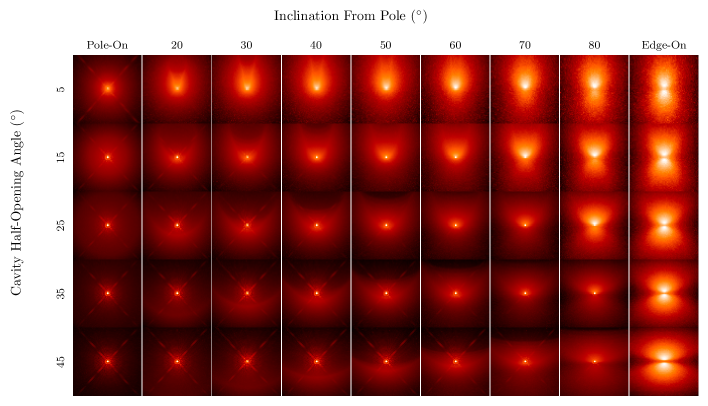
In order to quantify the shape of the observed cavities, we used a monochromatic Monte Carlo radiative transfer code, HO-CHUNK.ttsscat.20090521 (based on Whitney & Hartmann, 1992, 1993). With this code, we simulated $1.60\text{\,}\mathrm{\SIUnitSymbolMicro m}$ images of a half solar mass star surrounded by a flared disk, with a power-law radial density and scale height and an envelope, following the Terebey, Shu, and Cassen (TSC) model described in Terebey et al. (1984), (see also Ulrich, 1976, Cassen & Moosman, 1981). We examined six envelope densities (each corresponding to a different mass infall rate in Table 1), five cavity half-opening angles (see Figure 1 for the definition), five disk sizes, four disk masses, two variations on disk flaring and ten inclinations. Table 1 shows the parameters used in our model grid. All models adopt an identical photon flux from the central star and assume fully-evacuated cavities containing no material. These model images were convolved with the HST WFC3IR point spread function for the F160W filter. In this paper, we are primarily interested in variations in the observed near-IR morphology due to changes in envelope density, cavity half-opening angle, and inclination.

In these models, the mass infall rate is used as a parameter to control the densities of the envelopes. The infall rate is combined with an adopted central stellar mass of $0.5\text{\,}\mathrm{M_{\sun}}$ to scale the envelope density using Eqn. 3 from Kenyon et al. (1993). See Furlan et al. (2016) for further discussion on this scaling.

The disk and envelope dust opacities are from a model by Ormel et al. (2011) that adopts a 2:1 mixture of ice-coated silicates and bare graphite grains, where the depth of the ice coating is $10\text{\,}\mathrm{\char 37\relax}$ of the particle radius. The particles are subjected to time-dependent coagulation; we choose a coagulation time of $0.3\text{\,}\mathrm{Myr}$ . This is identical to the dust model used in Fischer et al. (2014) and Furlan et al. (2016). In the near-infrared, the opacities predicted by this model are slightly smaller than those of the often-cited OH5 opacities (Ossenkopf & Henning, 1994). The reasons for adopting this model are described in Furlan et al. (2016). In Appendix F, we assess the dependence of the cavity appearance on the dust law.

Motivated by the shape of the observed outflow cavities, we used a parabolic model ( $n=2$ ) shown in Figure 1 for outflow/envelope boundary in our models. In Section 4.2, we relax this constraint and use the power-law fit

z=A\left|\rho\right|^{n}

(1)

where the resulting power-law index, n, may be 1 or greater. For a given power-law, the cavity half-opening angle depends on the adopted outer radius of the envelope; only for the case of a conical cavity ( $n=1$ ) is the half-opening angle independent of the adopted outer radius.

Examples of models from the grid are shown in Figure 2, which displays the effect of differing inclinations and cavity half-opening angles. Several model parameters, such as the radius and temperature of the central protostar or the presence of hot spots, are not constrained by either the SEDs or the near-infrared images. The surface brightness found in an image depends on the monochromatic luminosity of the protostar (which in turn depends on the temperature, radius and presence of hot spots), but the morphology of the image depends primarily on envelope density, outflow cavity shape and inclination. The rest of our model parameters are chosen to cover a range of physical parameters observed in the fitting done by Furlan et al. (2016). This allows us to compare in Appendix G the values for the parameters determined by the fits to the SEDs and those determined from the near infrared images.

As shown by the models, the observed morphologies of the cavities trace the light scattered at a discontinuity in the dust density; in this case, the discontinuity is the boundary of a cleared cavity. If the protostar is seen edge-on, both cavities carved by the bipolar outflow are apparent. For these edge-on cases, a dust disk obscures the scattered light creating a dust lane (Figure 2). If the system is inclined such that the extinction toward the far cavity is significantly higher than that toward the nearer one, a bowl-shaped unipolar structure is seen due to the obscuration of the more distant cavity. The envelope itself can be directly illuminated if the density is low enough for near-infrared photons to penetrate past the cavity walls and scatter off grains deep in the envelope. In these cases, the disk can cast shadows in the envelope which are also apparent for edge-on inclinations.

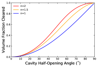
To compare our cavities to those measured in other analyses that adopt different models for their shapes (e.g. this work, Furlan et al., 2016, Arce & Sargent, 2006), we will determine the fraction of the envelope volume within the cavities. This is a measure of the amount of gas cleared by the outflow. The volume of the cavities in these models depends only on the power-law exponent $n$ , the half-opening angle $\theta$ and the outer envelope radius $R_{\text{max}}$ (Figure 1). In Figure 3, we show the dependence of the fraction of the envelope volume cleared by the cavity on the cavity half-opening angle and the cavity exponent.

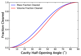
An alternative metric for characterizing cavity sizes is the fraction of the envelope mass cleared by the outflows, i.e. the fraction of mass that would be found in an initially spherical symmetric core with a $\rho^{-1.5}$ density law and an outer radius of 8000 AU. We compare the volume and mass fraction cleared in Figure 4. We find the fraction of the mass cleared can be up to $9\text{\,}\mathrm{\char 37\relax}$ more than the volume cleared, and that the volume cleared is a lower limit to the mass cleared. We note that this is an instantaneous mass fraction of the current envelope,and it will differ from the total fraction of the envelope mass entrained and ejected by the outflow over the history of a protostellar collapse. Furthermore, it does not include the mass launched and ejected from the system by disk winds, X-winds, or accretion-driven stellar winds (e.g. Watson et al., 2016).

4 Results

In this section, we classify the protostars on the basis of their $1.60\text{\,}\mathrm{\SIUnitSymbolMicro m}$ morphologies in the HST images. We then examine how the morphologies depend on the properties derived from the model fits to their SEDs. For protostars with detected outflow cavities, we develop an algorithm to measure the shape of the outflow cavity, and we calibrate this approach using the radiative transfer models in our grid.

We exclude the images with the F205W filter from this analysis as only the 83 objects successfully observed with NICMOS have these data. Furthermore, with a small number of exceptions, the morphologies are identical in the two NICMOS bands.

4.1 Protostellar Morphologies

The HST images resolve protostars at various stages of evolution, different inclinations and differing amounts of envelope material. In these images, light primarily from the photospheres of the central protostars is scattered by dust grains in the envelopes, delineating structures present in the envelopes. In many of the images, the structures are similar to those caused by the outflow cavities in our model grid.

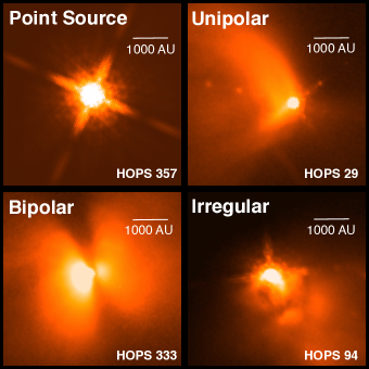
As a first step in our analysis, we divide all protostars into five morphological categories (Figure 5). The presence of a bipolar nebula, such as two scattered-light lobes separated by a dark lane or two outflow cavities, define the bipolar category. Sources with only one cavity visible make up the unipolar category. Unresolved protostars without detectable nebulosity are defined as point sources. Sources too deeply embedded to detect in the F160W band are considered non-detections (not shown in Figure 5). The final category comprises irregular protostars; these may result from background contamination (e.g., coincidence with a more extended reflection nebula), or true inhomogeneities in the structure of the protostellar envelope. For bipolar, unipolar and irregular categories, the presence of an unresolved point source in the nebula is noted; these are likely to be the central protostar or light scattering off of structures within 80 AU of the protostar, which is the smallest scale we can resolve in our images.

In total, 141 HOPS objects exhibit extended structures in scattered light. The classification of all protostars are found in Table 4, and their breakdown is summarized in Table 2. Of these, thirty-one show a bipolar structure indicative of an edge-on inclination, although some cases show the point source of the central protostar near or offset from the midplane of the dark lane, implying that they are not exactly edge-on. One bipolar source was serendipitously observed in the same field as HOPS 334. This source was first identified as a candidate protostar by Stutz et al. (2013); based on their values for $T_{\text{bol}}$ and $L_{\text{bol}}$ , it is determined by the criteria in Furlan et al. (2016) to be a Class 0 protostar. In this paper, we introduce this source into the HOPS catalog as HOPS 410 (Table 4). Fifty-nine objects show nebulosity appearing to be a cavity on one side, with 36 of those having detected point sources near the base of the cavity. Fifty-one remaining protostars are classified as irregular. Images of sources with unipolar, bipolar, irregular and point-like morphology are shown in Appendix A. Two additional Class II sources with nebulosity that were serendipitously discovered in our observation are shown in Appendix D.

Table 2: Breakdown of F160W morphologies

	Point	No Point	Total
	Source	Source
Non-detections	-	60+3	60+3³³3One of these three sources is likely an extragalactic source and two are of uncertain nature (Furlan et al., 2016).
Point Source⁴⁴4Sources without associated nebulosity	93+7	-	93+7⁵⁵5Six of these seven sources are likely extragalactic sources and one is of uncertain nature.
Irregular	39	12	51
Unipolar	36	23	59
Bipolar	16	15	31
Total	184+7	110+3	294+10⁶⁶6Includes seven likely extragalactic sources and three of uncertain nature.

Approximately half of our sample, 163 objects, have no resolvable nebulosity in these observations.⁷⁷7This includes objects identified as of uncertain nature or potential extragalactic contaminants by Furlan et al. (2016). One hundred of these are detected as one or more isolated point sources; these have been analyzed to determine the companion fractions throughout the Orion Molecular Clouds (Kounkel et al., 2016). We refer to these as point sources without associated nebulosity. In these cases, any nebulosity around the source appears to be part of an extended nebula that is illuminated by other stars in the region or is very faint and tenuous and does not delineate a clear structure around the point source. As we will discuss in Sec. 4.4, the scattered light from cavities and envelopes illuminated by these sources are likely too faint to detect against the PSF of the point source. The remainder of the sources are non-detections.

Emission along jets, most likely dominated by the [FeII] line at $1.66\text{\,}\mathrm{\SIUnitSymbolMicro m}$ , is observed in thirteen protostars, with three additional tentative detections. These are the bipolar protostars HOPS 133, 150, 186 and 216; the unipolar sources HOPS 29, (shown in Figure 5), HOPS 164 and 310; the irregular protostars HOPS 98, 188, 234 and 386; the point source 279 and the protostar HOPS 152, which although not detected directly at $1.60\text{\,}\mathrm{\SIUnitSymbolMicro m}$ , is situated at a location that is an apparent source of jet emission. Tentative detections of jets are found toward the point source protostars HOPS 3, 344 and 345.

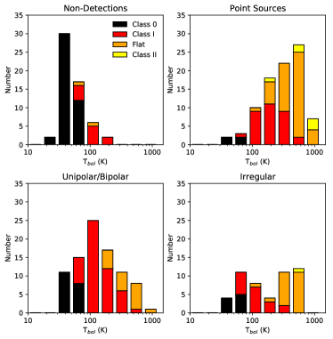
In Figure 6, we plot the number of protostars vs bolometric temperature for four morphological groups: non-detections, point sources, unipolar or bipolar sources, and protostars with irregular morphologies. The bolometric temperature is a measure of the evolutionary stage of the protostar, although it also has some dependence on inclination (Ladd et al., 1998, Furlan et al., 2016). We also include the standard evolutionary classes, as determined with the criteria in Furlan et al. (2016). These figures demonstrate the strong dependence of detectability and morphology in the near-IR with on the class of a protostar. The least evolved protostars (Class 0) are predominantly not detected due to the greater optical depths in their envelopes. In comparison, the most evolved sources (i.e., flat-spectrum protostars and Class II pre-main sequence stars) are dominated by unresolved point sources due to the low density of dust (and therefore low scattering probability) in their sparsely filled or non-existent envelopes.⁸⁸8Furlan et al. (2016) show that flat-spectrum protostars are a combination of protostars with higher density envelopes seen at low inclinations and protostars with lower envelope densities seen at any inclination. The first possibility is less common since it requires a limited range of inclinations. Protostars with unipolar and bipolar cavities show a broad range of $T_{\text{bol}}$ , but peak in the Class I phase ( $T_{\text{bol}}\sim$100\text{\,}\mathrm{K}$$ ) and contain a significant fraction of Class 0 objects. Finally, the irregular protostars consist largely of Class I and flat-spectrum sources.

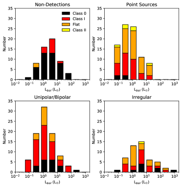
We show the distribution of bolometric luminosities for each morphological class in Figure 7. The luminosity distributions for the three non-irregular classes display a shift in median luminosity, with point sources, unipolar/bipolar protostars and non-detections having median $L_{\text{bol}}$ of $0.51.42.7\text{\,}\mathrm{L_{\sun}}$ , . This change is small compared to the full range of bolometric luminosities probed, from 0.05 to $480\text{\,}\mathrm{L_{\sun}}$ . It is likely due to a decline in the luminosity with increasing age, as found by Fischer et al. (2017).

4.2 Direct Measurements of Cavity Sizes

For protostars with unipolar or bipolar morphologies, we fit a power-law to the shape of the cavities to estimate the amount of the envelope which was cleared by the outflows. This analysis relies on a custom edge detection routine developed to locate the outer contours of the cavities in the images. The methodology is illustrated in Figure 8. It is similar to the Sobel filter described in Danielsson & Seger (1990), constrained to the dimension perpendicular to the axis of the cavity. The image is first rotated such that the cavity is aligned with the positive $y$ axis in an $x-y$ Cartesian plane; this defines our adopted axis for the cavity. In three bipolar cases, those of HOPS 136, 280 and 333, we were able to measure the shape of both cavities. For each image, a 1D Gaussian smoothing kernel was chosen by eye to account for noise and applied to every slice of constant $y$ . The width of the smoothing kernel is between 2 and 4 pixels, approximately $0.3\text{\,}\mathrm{\SIUnitSymbolArcsecond}$ .

We then calculate the second order finite difference along the slice (i.e. parallel to the $x$ -axis) using the equation

\frac{d^{2}I}{dx^{2}}=I(x+2)-2I(x+1)+I(x),

(2)

The inflection points allow us to define an “edge” of the cavity. The width of the smoothing kernel is increased to obtain a consistent edge, as a small smoothing kernel can produce a discontinuous edge. Inflection points are inspected to ensure that only those tracing the cavity (as opposed to structure within or outside the outflow cavity) are retained. More sophisticated techniques (e.g. Canny, 1986) have a limited advantage due to the presence of unrelated structures in the line of sight that cannot be treated as random noise.

To determine the half-width of the cavity, $x$ , at a given position along the cavity axis, $y$ , we measure the full width of the cavity between the two walls and then divide by two. Thus, the central axis of the outflow is defined by a curve tracing the midpoint of the two walls. Note that the $y$ position is the distance along a straight line that starts at the base of cavity and extends along the adopted cavity axis (Figure 8).

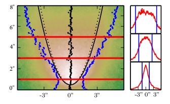
In order to relate the detected edge to the physical cavity in the envelope, we ran the edge detection routine on our model grid. We compared the edges measured for the models as a function of the observed inclination to the shape of the projected cavity wall for the same model as observed from an edge-on inclination; this allows us to correct for the effect of inclination of the shape of the outflow. The location of the projected wall is given by the analytic equation $y=A|x|^{n}$ (Figure 1).

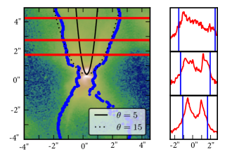
For most models, the detected edges of the cavities differ systematically from those of the projected wall (Figure 8); this is due to the combined effects of inclination, the penetration of the light from the central protostars past the cavity wall into the envelope and systematic biases of the edge detection routine. The inclination alone will broaden the cavity by $725\text{\,}\mathrm{\char 37\relax}$ for a $4060\text{\,}\mathrm{\SIUnitSymbolDegree}$ inclination assuming a parabolic cavity.

Figure 8 shows our edge fitting routine applied to a model image of a protostar with an inclination of $60 °$ and a cavity half-opening angle of $15 °$ . The black solid line indicate the projected cavity wall of this model, as observed from this inclination. The black dashed line indicates where the cavity wall would be for the same analytical shape, but observed at an edge-on inclination — almost negligible even for a $60 °$ inclination. The detected edges (in blue) are characteristically wider than the known cavity wall.

To quantify the difference between the observed and actual edge, we determined the ratio of the distance to the “detected” edge in the model to that of the known, projected distance to the wall. For a given model, this ratio was found to be approximately constant as a function of the distance along the outflow axis. Thus, a single ratio can describe the difference between the observed and actual outflow cavity for a given source. Using the grid of models described in Section 3, the ratio was measured as a function of the cavity half-opening angle and inclination.

At lower inclinations, the line of sight toward the central protostar is more likely to be directly into the cavity or to pass through less envelope material, thus significantly increasing the probability to observe the protostar as a point source (see Section 4.4). In these cases, the cavity walls are difficult to detect against the PSF. Additionally, because there exist more possible lines of sight toward edge-on or near edge-on orientations than pole-on or near pole-on orientations, the probability that a protostar will be observed at a given inclination decreases as inclination decreases, assuming that the cavity may face any direction randomly. For these reasons, we averaged the ratios determined from all models for each cavity size, considering only inclination angles from $90 °$ to $50 °$ . The ratios are displayed in Figure 9, which shows that they are predominantly constant as a function of half-opening angle except at the smallest opening angles and that they have a weak dependence on inclination. The standard deviation over all parameters aside from cavity size and inclination are shown as the error bars in this figure.

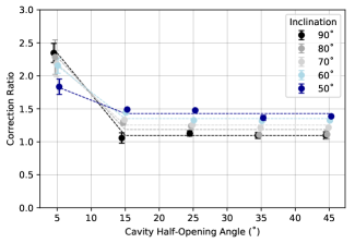
These ratios shown in Figure 9 were applied to the measured half-width of the cavities from the HST images. Generally, we initially divided the half-width by $1.3$ , which is the approximate average ratio for $50 °$ - $80 °$ inclination cavities with a half-opening angle greater than $15 °$ . For cavities of these sizes that were also bipolar and thus presumably near $90 °$ in inclination, we restricted our initial ratios to $1.1$ . For cavities with narrower opening angles and unipolar and bipolar morphologies, we chose initial ratios of $2.0$ and $2.3$ respectively. We then iterated when necessary, modifying the correction ratio until the combination of the ratio and recovered half-opening angle was consistent with combinations observed in our models, shown in Figure 9.

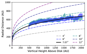
We fit the cavity width as a function of the distance along the outflow axis to the function

y=A|x-x_{0}|^{n}+y_{0}.

(3)

to both the model grid discussed in Section 3 and observed images (Figure 10). Here, $(x_{0},y_{0})$ identify the location of the protostar, and are fixed to the center of our model images. In the observed data, the parameters $(x_{0},y_{0})$ are manually centered on the central protostar when apparent from a point source or an area of maximum flux along the profile of the cavity or were placed along the disk absorption lane in the case of some bipolar sources. The midpoints of the cavity, as shown in Figure 11, were used to fit a center line which in turn allowed us to perform a final small-angle rotation correction. Our two detected edges were then considered for fitting in three ways: both the left and right edges were independently fit with a power-law profile, and, after folding over the now vertical center line, both detected edges were simultaneously fitted. This allowed us to counter minor asymmetries in detected cavity edges as well as outlying points biasing our fitting regime on a single edge. The recorded parameters were those given by the single-edge fit with an exponent $n$ greater than 1, or in cases where both edges met this criteria, the parameter from the folded fit was recorded. The exponent $n$ , which is referred to as the cavity exponent, gives a measure of the collimation of the outflow cavity and may be indicative of the physical mechanism behind the outflow creation. For example, Shu et al. (1991) show how a shell of molecular gas composed of the outflow and swept up material has a shape dependent on the angular distribution of the outflow.

By allowing $n$ to be an unconstrained free parameter in our fitting (with the caveat that it be greater than 1), we allow for conical cavities ( $n=1$ ) as well as parabolic cavities ( $n=2$ ). The amplitude $A$ parameterizes the size of the cavity. For the model used by the HO-CHUNK code, this relates the radius of the envelope ( $R_{\text{max}}$ ) and the cavity half-opening angle $\theta$ by:

A=R_{\text{max}}^{1-n}\cot^{n}\theta.

(4)

The value of $\theta$ is only dependent on $A$ for conical cavities ( $n=1$ ), but for other values of $n$ , the value of $\theta$ depends on our choice of $R_{\text{max}}$ , which we set to $8000\text{\,}\mathrm{AU}$ . Error analyses for functions of the fitted values are discussed in Appendix C.

For three protostars with bipolar morphologies, we were able to measure parameters for both cavities. In all other bipolar cases, the cavity appearing brighter was fitted. From our monochromatic model grid, we can see that inclination is responsible for variations in brightness between the two cavities. We expect the closer cavity to have a stronger signal due to a smaller extinction along the line of sight, although inhomogeneous envelopes may also be responsible for differences in cavity brightness.

An example of our fitting technique applied to the protostar HOPS 136 can be seen in Figure 11. Fischer et al. (2014) determined that this protostar is a late stage object with a $10\pm 2.\text{\,}\mathrm{\SIUnitSymbolDegree}$ half-opening angle for a $R_{\text{max}}=$10\,000\text{\,}\mathrm{AU}$$ envelope. The detected edges of its northern cavity are compared with power-law curves as given by Equation 3 in Figure 10, revealing the northern cavity of this protostar is best fit by a $8.7 °$ half-opening angle,⁹⁹9For the bipolar protostar HOPS 136, measurement of both the northern and southern cavity edges was possible. In Table 4, the average of both sets of parameters are reported. in close agreement with Fischer et al. (2014).

For thirty of the ninety protostars in our sample with unipolar or bipolar morphologies, we use this technique for measuring the cavity shape, and tabulate the values of $n$ in Table 4 along with the half-opening angle. The median uncertainty for $n$ , as obtained from the least squares fitting of Equation 3, is $\delta n\sim 0.14$ . We find from Equation C1 that uncertainties in half-opening angle measurements are on average $\delta\theta<$$$ . We also include in Table 4 the volume fraction of the envelope cleared by the cavity as in Section 3. We calculate this assuming a spherical envelope and a cavity volume given by the profile in Equation 3. For simplicity, we calculate the uncertainty in this measurement for the case of a conical cavity of the same half-opening angle. Uncertainties in this metric are $\sim$5\text{\,}\mathrm{\char 37\relax}$$ of the measured volume fraction (Appendix C). We note that these uncertainties describe the accuracy of our fits after carefully determining the axis of the outflow cavity and selecting regions for fitting over which our edge detection was well behaved and not confused by errant nebulosity, background stars, or the PSF of the central protostars. These determinations and selections may introduce systematic uncertainties that are not accounted for in the formal uncertainties.

The remaining sixty unipolar and bipolar protostars are excluded due to the inability to accurately and fully trace the cavity with the HST images. For several sources we see a morphology indicative of an edge-on or nearly edge-on disk but do not see evidence for a cavity (e.g. HOPS 65 and HOPS 200); these may be pre-main sequence stars with disks. Other protostars have cavities that are too faint to reliably trace (e.g. HOPS 220 and HOPS 235), show only one edge of a cavity wall - due to either a non-uniform extinction or an irregularly shaped envelope (e.g. HOPS 18 and HOPS 310), or are coincident with nebulosity - making it impossible to disentangle the cavity from larger scale structures (e.g. HOPS 387 and HOPS 384). Finally, some cavities exhibit morphologies inconsistent with a power-law cavity (e.g. HOPS 8 and HOPS 232). In general, the factors that prevented automated fitting appeared incidental and not obviously correlated with apparent cavity size. Future efforts will focus on expanding the range of brightness levels and morphologies analyzed as well as understanding the nature of cavities with only one apparent wall.

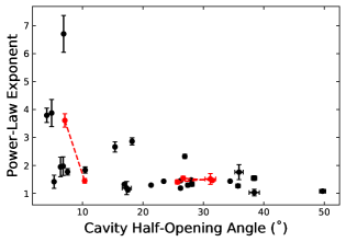
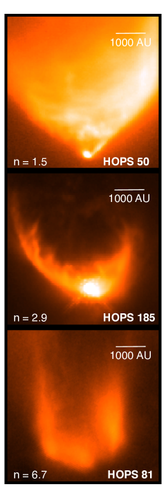
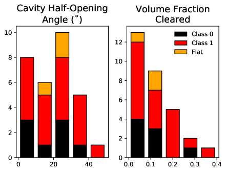
Figure 12 shows the range of fitted exponents $n$ and cavity half-opening angles measured in this work. We find the mean and median of the cavity exponents are $1.9$ and $1.5$ respectively, indicating that parabolic cavities are a reasonable model assumption. Cavity exponents vary significantly between the protostellar cavities; we show examples of this variation in Figure 13. Finally, we show our distribution of cavity half-opening angles and volume fractions in Figure 14.

4.3 Cavity Sizes vs. SED Derived Properties

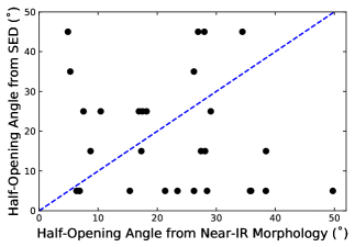
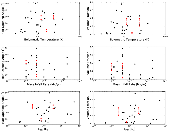
The SEDs of the protostars provide information on both their evolutionary phase as well as their total luminosity (e.g. Whitney et al., 2003). Correlations between the SED derived properties of protostars with the cavity sizes provide a means to probe the evolution of cavities as well as, potentially, their dependence on the final mass of the protostar (Fischer et al., 2017). Figure 15 shows two ways of parameterizing the cavity size, half-opening angle and volume fraction cleared, against an assortment of evolutionary indicators derived from the $1.6870\text{\,}\mathrm{\SIUnitSymbolMicro m}$ SED (Furlan et al., 2016). We calculate the half-opening angles with Equation 4 using the values of $A$ and $n$ and an envelope radius of $8000\text{\,}\mathrm{AU}$ .

We quantify the degree of correlation by finding the Spearman Rank Correlation Coefficient $r$ , a measure of the monotonic correlation between two variables in our thirty measured protostars. A correlation coefficient of 1 or -1 implies a strictly monotonic correlation. The Spearman coefficients and the two-sided $p$ -value for a hypothesis test are given in Table 3 for each of the diagnostic indicators and methods of parameterizing the cavity size. The hypothesis test uses a null hypothesis of no correlation; therefore, low $p$ -values indicate evidence of a correlation and evolutionary trend. For the three bipolar sources with both cavities measured, the found parameters of the two cavities were averaged before computing Spearman Coefficients and $p$ -values.

We do not find statistically significant correlation between cavity size and $T_{bol}$ or mass infall rate, (which should be considered a proxy for envelope density, as discussed in Section 3). As shown in Figure 14, the sample of protostars is dominated by Class I sources; at $1.60\text{\,}\mathrm{\SIUnitSymbolMicro m}$ , many Class 0 protostars are not detected, while flat-spectrum sources are often point sources or have irregular nebulosity (see Figure 6). Hence, these results can be primarily interpreted as a lack of evidence for an evolution in cavity properties across the Class I phase. The wide scatter in cavity sizes does not appear to be the result of evolution, but must depend on other environmental or intrinsic factors.

A higher correlation coefficient is found between cavity size and luminosity, with more luminous objects tending to have larger cavities; however, the p-values show that we cannot rule out the null hypothesis.

Table 3: Spearman Coefficients and

p

-values.

Evolutionary	vs Half-Opening Angle		vs Volume Fraction
Diagnostic	$r$	$p$ -value	$r$	$p$ -value
$T_{\text{bol}}$	0.24	0.20	0.23	0.21
$\dot{M}_{\text{infall}}$	0.16	0.41	0.12	0.52
$L_{\text{bol}}$	0.26	0.16	0.29	0.12

4.4 The Prevalance of Point Sources

We detect cavities towards 90 (30%) of our sample, while 100 (33%) are observed as point sources without nebulosity. Since protostars are surrounded by envelopes that scatter light, the substantial number of point sources without detected scattered-light nebulosity is surprising. In this section, we examine why the point source morphology is common and test whether the number of point sources implies an observational bias in our cavity size distribution.

Protostars may be observed as point sources without detected cavities in two primary cases. First, the central protostar is observed along a line of sight directly into the cavity. In this case the brightness of the PSF from the central protostar, which will not be attenuated by the envelope, can be significantly stronger than scattered light from surrounding cavity walls, which may only contribute a diffuse scattering around the bright protostar (Figure 2). Even if the line of sight grazes the cavity wall, the bright PSF can dominate over the nebulosity. Second, a low density envelope leads to a more diffuse, lower surface brightness cavity wall and a brighter point source; once again, the cavity may not be visible against the PSF. In both of these cases, the extended nebulosity often found in the Orion clouds can also hide the scattered light from the cavities.

The first case may lead to a bias against detecting large cavities. For envelopes with large cavities, the central protostar can be directly observed over a larger range of inclinations. Furthermore, since the walls of the cavity are further from the protostar, they will have systematically lower densities than narrower cavities and they will intercept less flux from the central star; consequently, the walls will be fainter and harder to detect for large cavities (Figure 2).

To determine the combinations of inclinations, cavity sizes and envelope densities that lead to the point source morphology, and to ascertain potential biases in our observed cavity size distribution, we use a Monte Carlo simulation that combines the model grid in Section 3, the envelope densities from the SED model fitting of Furlan et al. (2016) and several adopted cavity size distributions. The steps of the simulation are as follows.

We first determined for each model in our grid whether a cavity would be detected by the WFC3 observations. To determine whether a cavity is detectable, two criteria were applied to each model. Non-detections of cavities were noted when no distinct edge that delineates a cavity is found in the image using the technique of Section 4.2 or when the signal in a cut taken across the cavity $2000\text{\,}\mathrm{AU}$ from the central protostar has a peak value below the typical RMS of an image. At $2000\text{\,}\mathrm{AU}$ , every protostar with a detected cavity shows nebulosity; if the signal from the nebulosity in the models is below the typical RMS values in the WFC3 images, then it is unlikely that the cavity would be detected. The typical RMS was obtained from $30\text{\,}\mathrm{\SIUnitSymbolArcsecond}$\times$30\text{\,}\mathrm{\SIUnitSymbolArcsecond}$ off-source patches chosen to avoid point sources or outflow cavities. These patches commonly included extended, diffuse nebulosity that is common in the Orion Molecular Clouds.

We then performed a Monte Carlo simulation to predict the number of point sources without cavities we would detect for different assumed cavity half-opening angle distributions. We sampled the models drawing randomly for four parameters: infall rate (i.e. envelope density), inclination, inner F160W flux, and cavity half-opening angle. The distribution of infall rates for our sample of protostars (including those in the “irregular” category) were the best fit values in Furlan et al. (2016). Inclinations were drawn assuming the outflow axes were randomly oriented. The maximum disk radius, the mass of the disk and the radial exponent in the disk density law were left as free parameters to be randomly drawn from those in Table 1. The brightness in the inner 0.2" region for each model was determined by scaling the image flux to correspond to $1.60\text{\,}\mathrm{\SIUnitSymbolMicro m}$ magnitudes randomly drawn from the distribution of F160W magnitudes in the tabulation of Kounkel et al. (2016). Finally, we sampled the cavity half-opening angles from several different distributions discussed below.

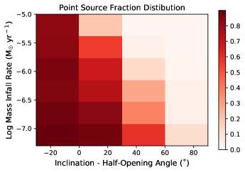
We plot the fraction of models resulting in point sources as a function of infall rate (i.e. envelope density), inclination and cavity half-opening angle in Figure 16. Here we subtract the cavity half-opening angle of a source from the inclination to measure the angle of the line of sight with respect to that of the cavity. Where this value is below zero, the line of sight is directly into the cavity and does not pass through the envelope. We find in Figure 16 a strong preference for point source morphologies in models observed at such inclinations and opening angles. When the inclination minus half-opening angle is positive and near zero, then the line of sight toward the central protostar intersects the lower density, outer regions of the envelope. In this case the incidence of a point source morphology increases with decreasing infall rate. Finally, if the infall rate is low, point source morphologies can be detected at every inclination and cavity half-opening angle combination, although the incidence increases at lower inclinations. As expected, point source morphologies arise when either the protostar is observed through its outflow cavity or when the envelope is thin. This is consistent with the point source morphology being dominated by protostars with flat-spectrum SEDs (Figure 6); the flat SEDs are expected for protostars observed at low inclinations or with low envelope densities (Calvet et al., 1994, Furlan et al., 2016).

Each iteration ¹⁰¹⁰10For each distribution of opening angles, we performed 30 thousand iterations. of the Monte-Carlo simulation returns the number of point sources without detected nebulosity. We compare this to the number of point sources in our data. Before comparing, we removed from our sample those sources identified by their SEDs as possible extragalactic contaminants or of an uncertain nature and those without complete SEDs (Furlan et al., 2016), except for sources where HST imaging has revealed a unipolar or bipolar morphology, confirming their protostellar nature. Seventeen sources observed with WFC3 and classified as either non-detections or point sources are removed based on these criteria. Finally, we choose only the point sources observed with WFC3, in order to account for differences in sensitivity. This reduces our sample down to 230 protostars, with 70 point sources.

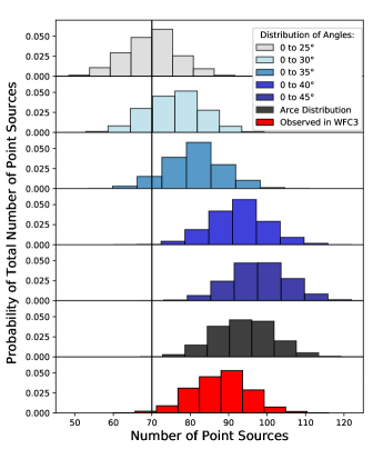
In Figure 17, we show normalized histograms of the number of point sources observed for various models of the cavity half-opening angle distributions. In red, we show the simulation results when the cavity sizes are randomly drawn from the values in Table 4. The observed number of point sources is marked with a vertical line. Realizations of 230 protostars with this simulation attain 70 point source detections or less of at rate of 1.02%. We note that our exclusion criteria, described above, reject 11 objects with point source morphologies from our sample. These objects could not be determined morphologically to be extragalactic contaminants, however, and were removed due to their SEDs. We note, however, that protostars may have extragalactic-like SEDs. HOPS 48, 67 and 301 were classified by Furlan et al. (2016) as extragalactic contaminants based on potential emission features in their Spitzer IRS spectra. In the case of these three sources, however, the features appear to originate in contamination from reflection nebulae or HII regions, and we observe cavities clearly associated with all three with HST WFC3. Thus we consider our observed number of 70 point sources to be a lower limit.

We also compare to fiducial models assuming a uniform distributions of cavities from 0 to 25, 30, 35, 40 and 45 degrees. The distributions extending beyond $35 °$ include enough large cavities to overpredict the number of point sources. These results indicate that our observations are not significantly biased against the detection of large cavity openings.

Finally, we examined the consequences of outflow cavities that grow with time. We first adopt the relationship between cavity half-opening angle and $T_{\text{bol}}$ found by Arce & Sargent (2006). We used this relationship and the observed distribution of bolometric temperatures of our protostars to derive the half-opening angle distribution we entitle “Arce Model.” We used a linear fit between the infall rate and $T_{\text{bol}}$ to pick a model in our grid on each iteration of the Monte Carlo. This model overpredicts the number of point sources, as it does not take into account the highly evolved protostars with low cavity half-opening angles found in our sample (e.g., Fischer et al., 2014).

In summary, we find that the histogram produced from the observed distribution overlaps with the observed number of sources, although with a 1% probability of predicting the predicted number of protostars or less. If some of our excluded contaminant sources are in fact protostellar in nature, the observed distribution may provide a better match. Importantly, the result here is that our observed cavity angle distribution is largely consistent with our observed number of point sources. Uniform distributions of half-opening angles extending to $45 °$ overpredict the number of point sources, and we do not find evidence that our observations fail to detect larger cavities. We also find that the uniform distributions with angles $<$$$ better reproduce the observed point sources than our observed distribution. This suggests that we may be missing small cavities that can be hard to detect due to higher extinction from their envelopes.

5 Discussion: Consequences for Protostellar Evolution

The goal of this study is to assess the impact of jets and winds on protostellar envelopes. This is an essential step toward both understanding how feedback lowers the efficiency of star formation and determining the importance of feedback in halting mass infall and setting the final masses of protostars. Feedback can lower efficiency and mass infall in three ways: by ejecting mass that would have otherwise been accreted, by clearing the envelope, and by entraining gas in the envelope and surrounding cloud into an outflow (e.g. Watson et al., 2016, Zhang et al., 2016). This paper aims to quantify the role of cavity clearing.

One way outflows may halt infall is by the progressive clearing of the envelope as the protostar evolves (Arce et al., 2013). This may be driven, for example, by successive bursts of a wide angle wind (Zhang et al., 2019). The signature of this clearing would be a correlation between cavity size and the evolution of the protostellar SEDs. We find no significant trend between cavity half-opening angle with either $T_{bol}$ or model inferred $\dot{M}$ , both indicators of envelope evolution (Section 4.3). Instead, we find that there is a range of cavity half-opening angles extending from $550\text{\,}\mathrm{\SIUnitSymbolDegree}$ present across the observed range of $T_{bol}$ and the range of $\dot{M}$ values inferred from model fits (Furlan et al., 2016). This implies that the evolution from dense to thin envelopes is not driven by the progressive growth of the outflow cavities.

To extend this result, we compare our cavity sizes with volume fractions calculated from millimeter and lower resolution IR studies in Figure 18. We use the tabulated outflow cavity angles and assumed conical cavity shapes to calculate the volume fractions. Our scattered-light measurements extend these by providing a relatively large sample at a common distance observed with a uniform spatial resolution, which eliminates possible biases due to distance, and by detecting a significant number of protostars with relatively high $T_{\text{bol}}$ ( $>$100\text{\,}\mathrm{K}$$ ) and smaller cavities ( $<$20\text{\,}\mathrm{\char 37\relax}$$ of the envelope cleared). The range of volume fractions (and hence, cavity half-opening angles) tabulated in the literature are consistent with those measured from our data, and there is no evidence for large systematic differences between the data sets, despite the different types of observations and methods used to measure the cavity sizes.

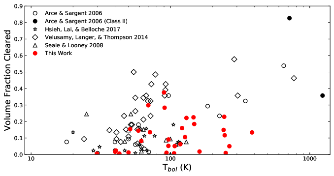
Arce & Sargent (2006) use millimeter line emission in the blue and red lobes identified in \ceCO maps to measure the cavity angle, assuming a conical outflow geometry. Although we do not share sources (so a direct comparison between the different methods cannot be made), we find that both the size scales probed and the range of observed volume fractions are similar, indicating that there are not large, systematic differences between the two techniques. Arce & Sargent (2006) suggest a correlation between an age diagnostic based on $T_{\text{bol}}$ and the cavity size. This correlation, however, is driven significantly by the Class II objects in their sample, shown in Figure 18. For instance, the Spearman Rank Correlation Coefficient of $T_{\text{bol}}$ and volume fraction decreases in their sample from 0.7 to 0.6 ( $p=0.0011$ to $p=0.015$ ) without the Class II objects. By definition, these objects only contain small remnants of their protostellar envelopes. They lack well-defined defined cavities, and the lack of envelopes may not necessarily be the result of clearing by progressively expanding outflows cavities.

Seale & Looney (2008) also measure the opening angles of envelope cavities in scattered light detected by Spitzer IRAC. Although this technique has a lower angular resolution than our study and encompasses a sample of objects spanning a much broader range of distances, it has the advantage of being able to detect outflow cavities from Class 0 objects which are apparent in the Spitzer $3.6\text{\,}\mathrm{\SIUnitSymbolMicro m}$ band. They also find correlation coefficients that indicate no or weak statistically significant correlation between cavity size and age indicators, with two exceptions. The first age indicator that is correlated with cavity size is the IRAC color (Figures 11b–d of that work), an indicator that may also depend on cavity size since larger cavities allow more radiation to escape at the wavelengths probed by IRAC. The second correlation is with the age parameter from the Robitaille et al. (2007) model grid. This age is used to set the sampling of cavity angles assuming cavity growth and thus could have induced a correlation. Sources from Seale & Looney (2008) with bolometric temperatures in the literature are plotted as triangles in Figure 18.

Other works have found evidence for cavity growth during the Class 0 phase, as suggested by Arce & Sargent (2006). Velusamy et al. (2014) measure the full opening angle near the base of the cavity using the HiRes reduction of Spitzer IRAC images. They find a broken power-law growth showing a clear increase in the sizes of cavities with increasing $T_{\text{bol}}$ from protostars with $T_{\text{bol}}<$100\text{\,}\mathrm{K}$$ , but do not reproduce the growth for more evolved objects.¹¹¹¹11The Velusamy et al. (2014) power-law breaks at an age of $8000\text{\,}\mathrm{yr}$ , as determined from $T_{bol}$ using the empirical relation of Ladd et al. (1998). This corresponds to a $\log{(T_{\text{bol}}/$\mathrm{K}$)}$ of $2\pm 0.25$ . Hsieh et al. (2017) also present a survey of low luminosity protostars using IRAC images, in addition to CFHT WIRCam Ks-band observations. These authors use the same radiative transfer modeling code described in Section 3, but they use a direct least-squares fit of their model grid to their images to determine the cavity parameters. They find evidence for a similar growth during the Class 0 phase. Although we do not find a similar correlation in our data, the Class 0 phase is dominated by non-detection in our $1.60\text{\,}\mathrm{\SIUnitSymbolMicro m}$ imaging and the smallest cavities will be harder to detect (Figure 6). Thus, we do not rule out the growth of cavities during the Class 0 phase.

Furlan et al. (2016), using the SEDs and modeling described in Section 4.3, find that the envelopes decrease in density by a factor of 50 as protostars transition from the Class 0 to the flat-spectrum phase. ¹²¹²12It is well recognized that the SED depends on both the inclination and the evolutionary stage, and the SED classes encompass a mixture of evolutionary stages. The SED classes, however, provide an approximate indicator of the evolution suitable for this analysis and has the advantage that they are not model dependent. See Robitaille et al. (2007) and Furlan et al. (2016) for further discussion. By the end of the Class I phase, it is thought that most of the stellar mass has been accreted. We should therefore expect the processes that reduce the mass and density of the protostellar envelope to continue through the Class I phase after starting in the Class 0 phase.

The lack of a correlation between the fraction of the volume cleared and the evolutionary indicators, in a sample preferentially probing Class I objects, implies that the evolution of the envelope during the Class I phase is not driven by growth of the outflow cavities. Although envelope clearing contributes up to a $40\text{\,}\mathrm{\char 37\relax}$ reduction, the more than an order of magnitude drop in the envelope density cannot be explained by this clearing alone. Of particular importance are the number of protostars with $<$15\text{\,}\mathrm{\char 37\relax}$$ of the envelope cleared throughout the entire range of $T_{\text{bol}}$ covered. One of the best examples is the protostar HOPS 136, which has a volume cleared of $1.8\text{\,}\mathrm{\char 37\relax}$ . Fischer et al. (2014) found that this protostar was in the late stages of stellar formation. The envelope mass of $0.06\text{\,}\mathrm{M_{\sun}}$ was much smaller than the estimated stellar mass of $0.40.5\text{\,}\mathrm{M_{\sun}}$ , showing that most of the stellar mass has been accreted. A relatively low density envelope is inferred from both the SED and the detection of scattered light in the envelope in the HST images (which implies a low optical depth at $1.60\text{\,}\mathrm{\SIUnitSymbolMicro m}$ ). The presence of such protostars with a low density, low mass envelope, and narrow outflow cavities at the late stages of stellar formation are clear examples where the clearing of the envelopes by outflows cannot explain the observed low envelope densities.

Our results also put limits on the ability of feedback from outflows to explain the low star formation efficiency. Comparisons of the Core Mass Function and Initial Mass Function suggest that $6070\text{\,}\mathrm{\char 37\relax}$ of the core mass will not accrete onto stars (Alves et al., 2007, Könyves et al., 2015), and previous authors have invoked outflows as partially responsible for this effect (e.g., Alves et al., 2007). Assuming the growth of the cavities is monotonic in time, the volume fraction cleared provides a lower limit on the mass fraction cleared by the outflows. From our HST data, the Class I protostars have cleared at most $40\text{\,}\mathrm{\char 37\relax}$ of their volume (Figure 18). Recalling that the mass fraction cleared from a cavity may be as much as $9\text{\,}\mathrm{\char 37\relax}$ higher than the volume cleared (Figure 4), the maximum fraction of mass cleared is $50\text{\,}\mathrm{\char 37\relax}$ . Most of the protostars have cleared a much smaller mass fraction, even those toward the end of their protostellar phase; the median volume fraction cleared for the HST sample is only $10\text{\,}\mathrm{\char 37\relax}$ . These results suggest that the feedback via clearing is not sufficient to explain the small star formation efficiency inferred for dense cores, and other mechanisms should be investigated.

There are other possible ways outflows may reduce star formation efficiency. The gas launched by the star-disk system in a jet or wind can escape the protostar and its envelope. Using estimates of the mass loss rates of 84 protostars, Watson et al. (2016) found that the median fraction of gas launched is $0.09$ of the gas accreted (although with a wide dispersion); this may decrease the star formation efficiency by up to an additional $10\text{\,}\mathrm{\char 37\relax}$ . We find a median star formation efficiency of $\sim$ $70\text{\,}\mathrm{\char 37\relax}$ given a $10\text{\,}\mathrm{\char 37\relax}$ median volume fraction cleared, a $9\text{\,}\mathrm{\char 37\relax}$ increase for mass fraction cleared, and an additional $10\text{\,}\mathrm{\char 37\relax}$ for mass directly launched and ejected by the central protostar. Only for the largest cavities, which clear up to $\sim$ $40\text{\,}\mathrm{\char 37\relax}$ of their envelopes, can the efficiency be as low as $\sim$ $40\text{\,}\mathrm{\char 37\relax}$ .

Secondly, the size of the cavity seen in scattered light may not measure the entire volume of the gas entrained in the outflow. In support of this, Seale & Looney (2008) noticed a possible discrepancy between their scattered-light outflow cavity sizes and the extent of the outflowing gas traced by millimeter line data. This outflowing gas may be slower moving, denser gas entrained into the outflow that is located outside of the cavities.

In the case of the HH46/47 outflow, Zhang et al. (2016) used ALMA data in the ¹²CO, ¹³CO, and C¹⁸O lines to measure the mass in the outflow, including the slower, denser, entrained gas. They find that the gas mass in the outflow with velocities exceeding the escape velocity is $\sim 3$ times the current stellar mass. If this instantaneous efficiency persists throughout the protostellar collapse, then the entrainment of gas in the outflow may account for the observed inefficiency. Simulations of collapsing cores with turbulence have also been able to achieve star formation efficiencies of 40% (Offner & Arce, 2014). Radiative transfer models based on these simulations are needed to predict the evolution of cavities and compare them to the cavities measured in this work.

Finally, if outflows are not sufficient to reduce star formation efficiencies to the observed levels or to slow/halt accretion, then other mechanisms must be identified. For example, the collapse of a finite Bonner-Ebert core leads to an exponential tapering in the infall rate (Vorobyov, 2010); however, this does not explain the inferred low star formation efficiency of cores. Furthermore, protostellar cores embedded in molecular clouds can draw gas from their surroundings and may not be limited by the mass in the surrounding core (Myers, 2009). Oscillating molecular filaments, as suggested by Stutz & Gould (2016) and Stutz (2018) may eject protostars. Alternatively dynamical interactions in small non-hierarchical systems or clusters may also eject protostars (Reipurth et al., 2010, Bate, 2012). Identifying this mechanism should be considered a key problem in star formation since it plays an important role in determining both the masses of stars and the efficiency of star formation.

6 Summary

We present WFC3 $1.60\text{\,}\mathrm{\SIUnitSymbolMicro m}$ and NICMOS $1.60\text{\,}\mathrm{\SIUnitSymbolMicro m}$ and $2.05\text{\,}\mathrm{\SIUnitSymbolMicro m}$ images of 304 protostars and pre-main sequence stars in the Orion Molecular Clouds. All of these objects were studied as part of the Herschel Orion Protostar Survey (HOPS) and are well characterized by their $1.6870\text{\,}\mathrm{\SIUnitSymbolMicro m}$ SEDs (Furlan et al., 2016). In this work, we use the images to resolve light from the central protostar scattered by dust in the envelopes surrounding the protostars, allowing us to probe structures with approximately $80\text{\,}\mathrm{AU}$ spatial resolution. The specific results are as follows:

•

We divide the sample into five distinct morphological classes. These morphological classes are non-detections (63), point sources without nebulosity (100), protostars with unipolar cavities (59), protostars with bipolar cavities (31), and irregular protostars (51). Thirteen of these protostars have jets appearing to originate from the protostars, and an additional three have tentative detections of jets. The relative incidence of each morphology depends on SED class: non-detections are dominated by Class 0 objects, protostars with cavities are dominated by Class I objects and the point sources are primarily composed of flat-spectrum and Class I protostars. The irregular morphological class contains a relatively even mixture of Class 0, Class I and flat-spectrum protostars. We find that non-detections have the highest bolometric luminosities while point-sources have the lowest.
•

For the protostars with observed cavities, we developed an edge detection routine to find the structure of the cavity walls. From this, we fit a power-law to the cavity shape and find the best fit shape (e.g., conical, parabolic, etc.) for 30 protostars in our sample with unipolar or bipolar morphologies. We calibrated this technique against our large model grid to reliably measure the opening of cavities. We find a distribution of cavity angles ranging from $4.149.7\text{\,}\mathrm{\SIUnitSymbolDegree}$ , while the power-law exponent varies from $1.1$ to $6.7$ with a median of $1.5$ . We note that these cavity angles are not correlated with the SED derived angles of Furlan et al. (2016), demonstrating that fitting radiative transfer models to SEDs does not provide reliable constraints on cavity sizes (Appendix G).
•

Using the well characterized SEDs of Furlan et al. (2016), we look for correlations between the observed cavity half-opening angle and evolutionary diagnostics such as SED class and bolometric temperature. Our data show no evidence for a dependence of outflow half-opening angle and volume fraction cleared with any of the evolutionary indicators. Furthermore, several evolved protostars with relatively small cavity sizes are identified. We conclude that there is no systematic growth of the cavity half-opening angle during the Class I phase.
•

We find that the incidence of point sources is consistent with both the observed cavity angle distribution and the distribution of envelope densities from Furlan et al. (2016). This implies that the point sources are protostars observed through a line of sight passing through the outflow cavity (hence seeing the protostar directly) or protostars with lower envelope density (as are typical of flat-spectrum protostars). Furthermore, we show that the number of point sources is inconsistent with a significant population of large cavities missed by our survey. Instead, our sensitivity to detecting cavities may decrease toward the smallest opening angles. As a whole, this is evidence that the cavity size distribution we obtain is reasonably complete and representative of the true distribution.
•

Our findings indicate that outflow clearing is not the primary mechanism for the dissipation of the envelope during the Class I phase. It further suggests that clearing alone cannot explain the $\sim$3040\text{\,}\mathrm{\char 37\relax}$$ star formation efficiencies inferred from core mass functions. Current measurements of the amount of mass directly launched by protostar in winds or jets suggest that this additional factor is not sufficient. Measurements of the molecular gas with millimeter interferometry are needed to determine whether slower, higher density flows entrained by the outflows are responsible for the halting of infall/accretion and the $\sim$3040\text{\,}\mathrm{\char 37\relax}$$ star formation efficiencies. If they are not, mechanisms other than feedback may be required.

Based on observations made with the NASA/ESA Hubble Space Telescope, obtained at the Space Telescope Science Institute, which is operated by the Association of Universities for Research in Astronomy, Inc., under NASA contract NAS 5-26555. These observations are associated with program #11548. Support for programs #11548, #14181 and #14695 was provided by NASA through a grant from the Space Telescope Science Institute, which is operated by the Association of Universities for Research in Astronomy, Inc., under NASA contract NAS 5-26555.

References

Adams & Shu (1985) Adams, F. C., & Shu, F. H. 1985, The Astrophysical Journal, 296, 655
Allen et al. (2002) Allen, L. E., Myers, P. C., Di Francesco, J., et al. 2002, The Astrophysical Journal, 566, doi:10.1086/338128
ALMA Partnership et al. (2015) ALMA Partnership, Brogan, C. L., Pérez, L. M., et al. 2015, The Astrophysical Journal Letters, 808, L3
Alves et al. (2007) Alves, J., Lombardi, M., & Lada, C. J. 2007, Astronomy and Astrophysics, 462, L17
Andre et al. (1993) Andre, P., Ward-Thompson, D., & Barsony, M. 1993, The Astrophysical Journal, 406, 122
Arce et al. (2013) Arce, H. G., Mardones, D., Corder, S. A., et al. 2013, The Astrophysical Journal, 774, doi:10.1088/0004-637X/774/1/39
Arce & Sargent (2006) Arce, H. G., & Sargent, A. I. 2006, The Astrophysical Journal, 646, 1070
Bate (2012) Bate, M. R. 2012, Monthly Notices of the Royal Astronomical Society, 419, doi:10.1111/j.1365-2966.2011.19955.x
Calvet et al. (1994) Calvet, N., Hartmann, L., Kenyon, S. J., & Whitney, B. A. 1994, ApJ, 434, 330
Canny (1986) Canny, J. 1986, IEEE Transactions on Pattern Analysis and Machine Intelligence, PAMI-8, 679
Cassen & Moosman (1981) Cassen, P., & Moosman, A. 1981, Icarus, 48, 353
Curtis et al. (2010) Curtis, E. I., Richer, J. S., Swift, J. J., & Williams, J. P. 2010, Monthly Notices of the Royal Astronomical Society, 408, doi:10.1111/j.1365-2966.2010.17214.x
Danielsson & Seger (1990) Danielsson, P.-E., & Seger, O. 1990, in Machine Vision for Three-Dimensional Scenes, ed. H. Freeman (Academic Press), 347–379
Dipierro et al. (2015) Dipierro, G., Price, D., Laibe, G., et al. 2015, Monthly Notices of the Royal Astronomical Society: Letters, 453, L73
Dunham et al. (2014) Dunham, M. M., Arce, H. G., Mardones, D., et al. 2014, ApJ, 783, 29
Dunham et al. (2013) Dunham, M. M., Arce, H. G., Allen, L. E., et al. 2013, AJ, 145, 94
Dunham et al. (2014) Dunham, M. M., Stutz, A. M., Allen, L. E., et al. 2014, Protostars and Planets VI, 195
Fischer et al. (2014) Fischer, W. J., Megeath, S. T., Tobin, J. J., et al. 2014, The Astrophysical Journal, 781, 123
Fischer et al. (2017) Fischer, W. J., Megeath, S. T., Furlan, E., et al. 2017, The Astrophysical Journal, 840, 69
Frank et al. (2014) Frank, A., Ray, T. P., Cabrit, S., et al. 2014, Protostars and Planets VI
Furlan et al. (2016) Furlan, E., Fischer, W. J., Ali, B., et al. 2016, ArXiv e-prints
Großschedl et al. (2018) Großschedl, J. E., Alves, J., Meingast, S., et al. 2018, A&A, 619, A106
Hansen et al. (2012) Hansen, C. E., Klein, R. I., McKee, C. F., & Fisher, R. T. 2012, The Astrophysical Journal, 747, doi:10.1088/0004-637X/747/1/22
Hatchell et al. (2007) Hatchell, J., Fuller, G. A., & Richer, J. S. 2007, Astronomy and Astrophysics, 472, doi:10.1051/0004-6361:20066467
Hsieh et al. (2017) Hsieh, T.-H., Lai, S.-P., & Belloche, A. 2017, The Astronomical Journal, 153, 173
Hunter (2007) Hunter, J. D. 2007, Computing in Science & Engineering, 9, 90
Kenyon et al. (1993) Kenyon, S. J., Calvet, N., & Hartmann, L. 1993, The Astrophysical Journal, 414, 676
Könyves et al. (2015) Könyves, V., André, P., Men’shchikov, A., et al. 2015, Astronomy and Astrophysics, 584
Kounkel et al. (2016) Kounkel, M., Megeath, S. T., Poteet, C. A., Fischer, W. J., & Hartmann, L. 2016, ArXiv e-prints
Kounkel et al. (2018) Kounkel, M., Covey, K., Suárez, G., et al. 2018, AJ, 156, 84
Krist et al. (2011) Krist, J. E., Hook, R. N., & Stoehr, F. 2011, Society of Photo-Optical Instrumentation Engineers (SPIE) Conference Series, 8127
Ladd et al. (1998) Ladd, E. F., Fuller, G. A., & Deane, J. R. 1998, The Astrophysical Journal, 495, 871
Lee et al. (2001) Lee, C.-F., Stone, J. M., Ostriker, E. C., & Mundy, L. G. 2001, The Astrophysical Journal, 557, 429
Machida & Hosokawa (2013) Machida, M. N., & Hosokawa, T. 2013, Monthly Notices of the Royal Astronomical Society, 431, doi:10.1093/mnras/stt291
Machida & Matsumoto (2012) Machida, M. N., & Matsumoto, T. 2012, Monthly Notices of the Royal Astronomical Society, 421, doi:10.1111/j.1365-2966.2011.20336.x
Matzner & McKee (1999) Matzner, C. D., & McKee, C. F. 1999, The Astrophysical Journal, 526, doi:10.1086/312376
Megeath et al. (2012) Megeath, S. T., Gutermuth, R., Muzerolle, J., et al. 2012, The Astronomical Journal, 144, 192
Megeath et al. (2016) —. 2016, The Astronomical Journal, 151, doi:10.3847/0004-6256/151/1/5
Myers (2009) Myers, P. C. 2009, The Astrophysical Journal, 706, 1341
Myers & Ladd (1993) Myers, P. C., & Ladd, E. F. 1993, The Astrophysical Journal Letters, 413, L47
Offner & Arce (2014) Offner, S. S. R., & Arce, H. G. 2014, The Astrophysical Journal, 784, doi:10.1088/0004-637X/784/1/61
Offner & Chaban (2017) Offner, S. S. R., & Chaban, J. 2017, ApJ, 847, 104
Oliphant (2007) Oliphant, T. E. 2007, Computing in Science Engineering, 9, 10
Ormel et al. (2011) Ormel, C. W., Min, M., Tielens, A. G. G. M., Dominik, C., & Paszun, D. 2011, A&A, 532, A43
Ossenkopf & Henning (1994) Ossenkopf, V., & Henning, T. 1994, Astronomy and Astrophysics 291, 943-959 (1994)
Padgett et al. (1999) Padgett, D. L., Brandner, W., Stapelfeldt, K. R., & Krist, J. E. 1999, American Astronomical Society Meeting Abstracts, 195
Raga & Cabrit (1993) Raga, A., & Cabrit, S. 1993, Astronomy and Astrophysics, 278
Reipurth et al. (2010) Reipurth, B., Mikkola, S., Connelley, M., & Valtonen, M. 2010, ApJ, 725, L56
Robitaille et al. (2007) Robitaille, T. P., Whitney, B. A., Indebetouw, R., & Wood, K. 2007, The Astrophysical Journal Supplement Series, 169, 328
Seale & Looney (2008) Seale, J. P., & Looney, L. W. 2008, The Astrophysical Journal, 675, 427
Shu et al. (1991) Shu, F. H., Ruden, S. P., Lada, C. J., & Lizano, S. 1991, The Astrophysical Journal, 370, L31
STSCI Development Team (2012) STSCI Development Team. 2012, DrizzlePac: HST image software, , , ascl:1212.011
Stutz (2018) Stutz, A. M. 2018, MNRAS, 473, 4890
Stutz & Gould (2016) Stutz, A. M., & Gould, A. 2016, A&A, 590, A2
Stutz et al. (2013) Stutz, A. M., Tobin, J. J., Stanke, T., et al. 2013, The Astrophysical Journal, 767, doi:10.1088/0004-637X/767/1/36
Terebey et al. (2006) Terebey, S., Buren, D. V., Brundage, M., & Hancock, T. 2006, The Astrophysical Journal, 637, 811
Terebey et al. (1984) Terebey, S., Shu, F. H., & Cassen, P. 1984, The Astrophysical Journal, 286, 529
The Astropy Collaboration et al. (2013) The Astropy Collaboration, Robitaille, T. P., Tollerud, E. J., et al. 2013, Astronomy & Astrophysics, 558, 9
Tobin et al. (2007) Tobin, J. J., Looney, L. W., Mundy, L. G., Kwon, W., & Hamidouche, M. 2007, The Astrophysical Journal, 659, doi:10.1086/512720
Tobin et al. (2016) Tobin, J. J., Stutz, A. M., Manoj, P., et al. 2016, ApJ, 831, 36
Ulrich (1976) Ulrich, R. K. 1976, The Astrophysical Journal, 210, 377
Velusamy et al. (2014) Velusamy, T., Langer, W. D., & Thompson, T. 2014, The Astrophysical Journal, 783, 6
Vorobyov (2010) Vorobyov, E. I. 2010, The Astrophysical Journal, 713, doi:10.1088/0004-637X/713/2/1059
Walt et al. (2011) Walt, S. v. d., Colbert, S. C., & Varoquaux, G. 2011, Computing in Science Engineering, 13, 22
Watson et al. (2016) Watson, D. M., Calvet, N. P., Fischer, W. J., et al. 2016, The Astrophysical Journal, 828, doi:10.3847/0004-637X/828/1/52
Whitney & Hartmann (1992) Whitney, B. A., & Hartmann, L. 1992, ApJ, 395, 529
Whitney & Hartmann (1993) —. 1993, ApJ, 402, 605
Whitney et al. (2003) Whitney, B. A., Wood, K., Bjorkman, J. E., & Wolff, M. J. 2003, The Astrophysical Journal, 591, 1049
Ybarra et al. (2006) Ybarra, J. E., Barsony, M., Haisch, K. E., et al. 2006, The Astrophysical Journal, 647, doi:10.1086/507449
Zhang et al. (2016) Zhang, Y., Arce, H. G., Mardones, D., et al. 2016, The Astrophysical Journal, 832, 158
Zhang et al. (2019) Zhang, Y., Arce, H. G., Mardones, D., et al. 2019, ApJ, 883, 1

\onecolumngrid

Appendix A Images of All Protostars

The images in this appendix show the NICMOS and WFC3 images of protostars which display bipolar or unipolar morphologies, are point sources without associated nebulosity, or are classified as irregular.

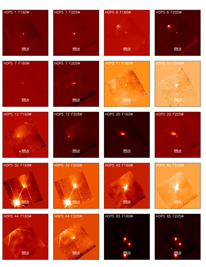
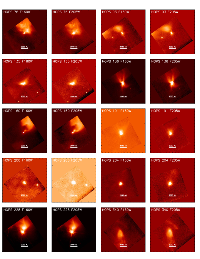
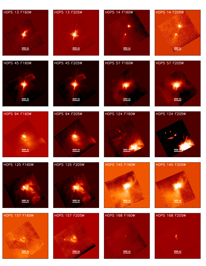
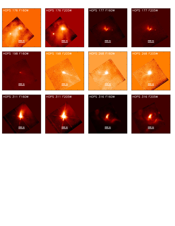
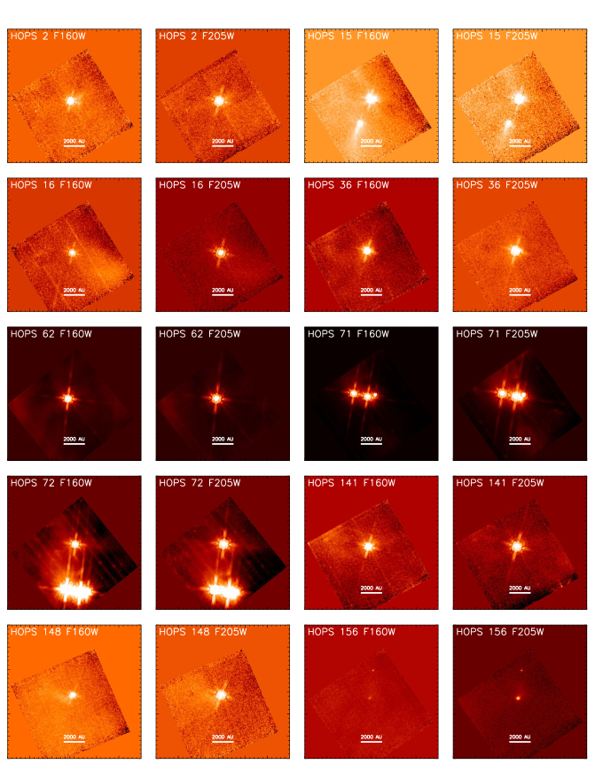
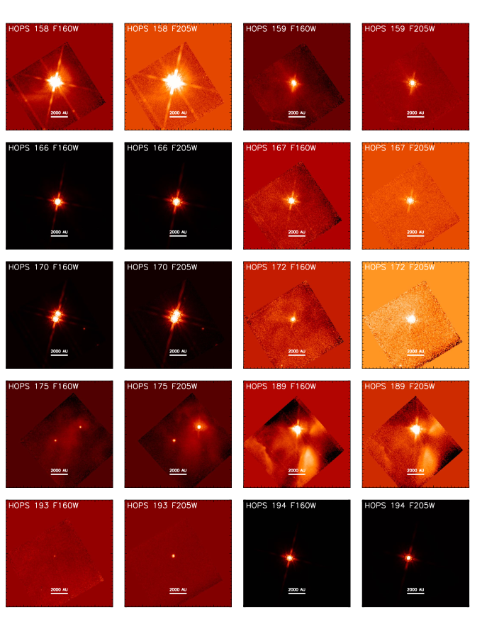
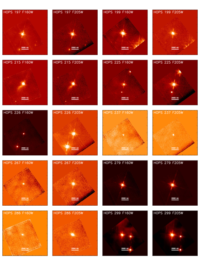
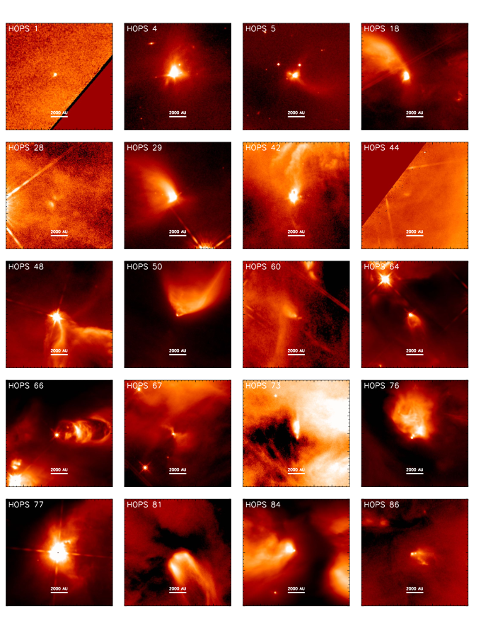
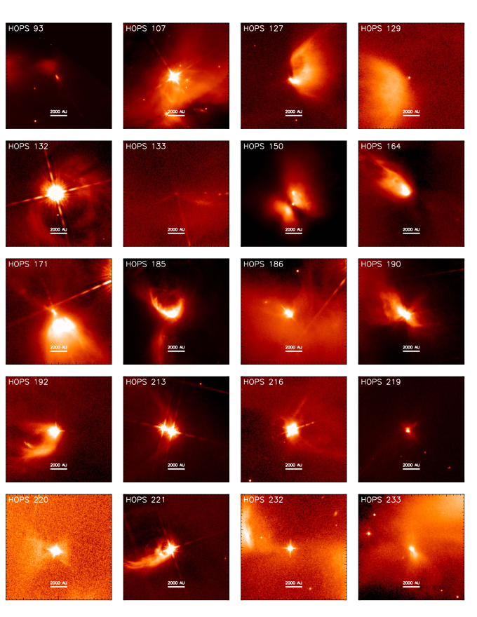
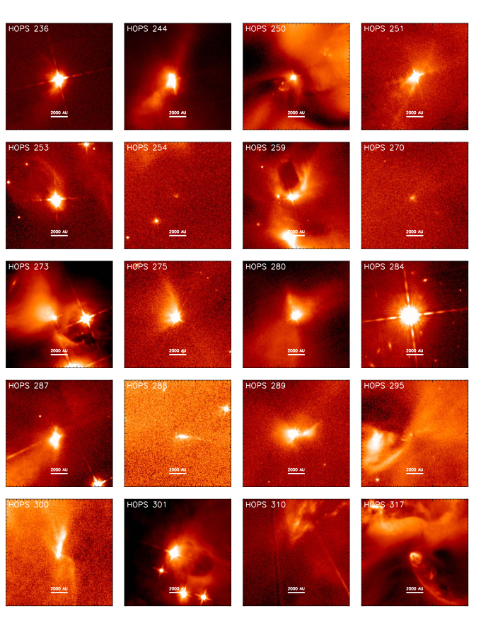
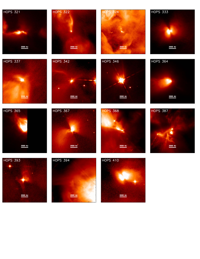
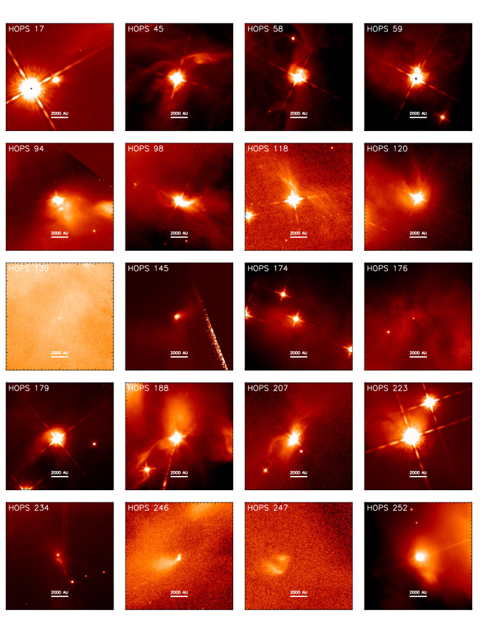
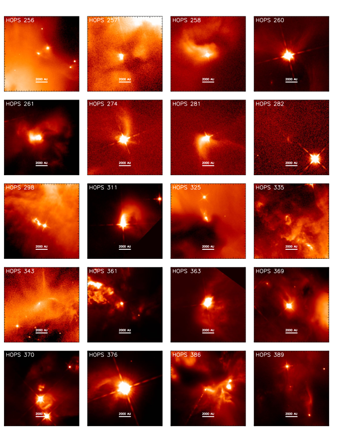
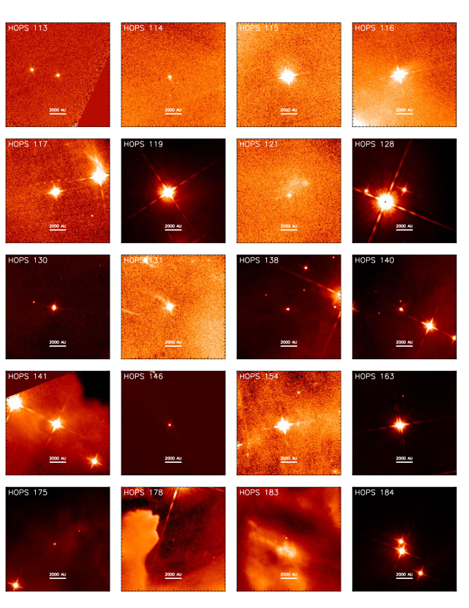
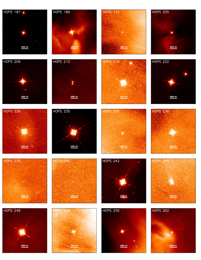
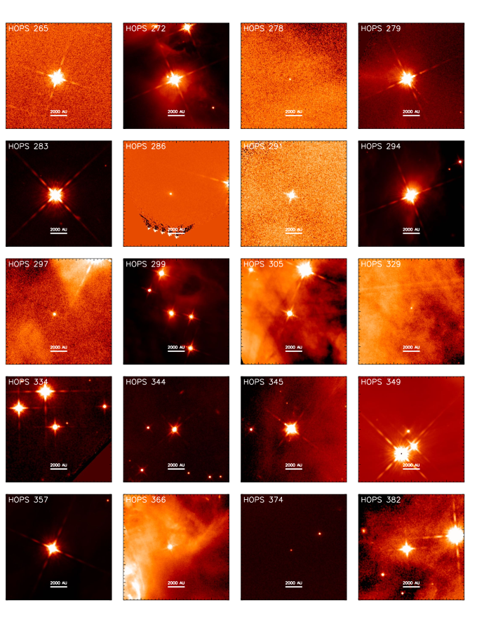
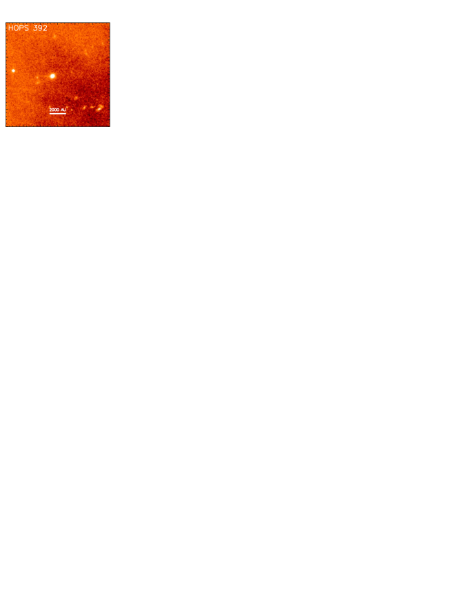
Appendix B Table of All HST Sources in this Text

Table 4:

HOPS	RA	DEC	SED	$T_{\text{bol}}$ ¹¹ Furlan et al. (2016)	Instrument²² Objects observed with the instrument NICMOS are noted with the abbreviation "NIC."	Point	F160W	Volume	Half-Opening	Power-
ID	ICRS		Class¹¹ Furlan et al. (2016)			Source³³ Denotes, (yes or no), if the object is observed with an apparent central point source.	Morphology	Cleared	Angle	Law Fit
				( $\mathrm{K}$ )				(%)	(^∘)	n
1	$05:54:12.3$	$+01:42:35$	I	72.6	NIC WFC3	n	Unipolar	-	-	-
2	$05:54:09.1$	$+01:42:52$	I	356.5	NIC	y	Point Source	-	-	-
3	$05:54:56.9$	$+01:42:56$	flat	467.5	WFC3	y	Point Source	-	-	-
4	$05:54:53.7$	$+01:47:09$	I	203.3	WFC3	y	Unipolar	-	-	-
5	$05:54:32.1$	$+01:48:07$	I	187.1	WFC3	y	Unipolar	-	-	-
6	$05:54:18.4$	$+01:49:03$	I	112.5	NIC	y	Unipolar	-	-	-
7	$05:54:20.0$	$+01:50:42$	0	58.0	NIC	n	Bipolar	-	-	-
10	$05:35:09.0$	$-05:58:27$	0	46.2	NIC	n	Non Detection	-	-	-
11	$05:35:13.4$	$-05:57:58$	0	48.8	NIC	n	Unipolar	-	-	-
12	$05:35:08.6$	$-05:55:54$	0	42.0	NIC	n	Unipolar	-	-	-
13	$05:35:24.5$	$-05:55:33$	flat	383.6	NIC	y	Irregular	-	-	-
14	$05:36:19.1$	$-05:55:30$	flat	464.0	NIC	y	Irregular	-	-	-
15	$05:36:19.0$	$-05:55:25$	flat	342.0	NIC	y	Point Source	-	-	-
16	$05:35:00.8$	$-05:55:25$	flat	361.0	NIC	y	Point Source	-	-	-
17	$05:35:07.1$	$-05:52:05$	I	341.3	WFC3	y	Irregular	-	-	-
18	$05:35:05.4$	$-05:51:54$	I	71.8	WFC3	n	Unipolar	-	-	-
20	$05:33:30.7$	$-05:50:41$	I	94.8	NIC	y	Unipolar	-	-	-
21	$05:36:10.1$	$-05:50:08$	ex	584.5	WFC3	y	Point Source	-	-	-
24	$05:34:46.9$	$-05:44:50$	I	288.9	WFC3	y	Point Source	-	-	-
26	$05:35:17.3$	$-05:42:14$	II	1124.9	WFC3	y	Point Source	-	-	-
28	$05:34:47.2$	$-05:41:55$	0	46.3	WFC3	n	Bipolar	-	-	-
29	$05:34:49.0$	$-05:41:42$	I	148.2	WFC3	y	Unipolar	18.4	26.9	2.3
30	$05:34:44.0$	$-05:41:25$	I	81.2	NIC WFC3	n	Non Detection	-	-	-
31	$05:35:17.2$	$-05:40:26$	flat	634.7	WFC3	y	Point Source	-	-	-
32	$05:34:35.4$	$-05:39:59$	0	58.9	NIC	n	Unipolar	14.4	28.1	1.3
35	$05:35:19.9$	$-05:39:01$	I	305.2	WFC3	y	Point Source	-	-	-
36	$05:34:26.4$	$-05:37:40$	flat	374.6	NIC	y	Point Source	-	-	-
38	$05:35:04.7$	$-05:37:12$	0	58.5	WFC3	n	Non Detection	-	-	-
40	$05:35:08.5$	$-05:35:59$	0	38.1	WFC3	n	Non Detection	-	-	-
41	$05:34:29.4$	$-05:35:42$	I	82.3	NIC	n	Non Detection	-	-	-
42	$05:35:05.0$	$-05:35:40$	I	200.9	NIC WFC3	n	Bipolar	-	-	-
43	$05:35:04.5$	$-05:35:14$	I	75.0	NIC WFC3	n	Non Detection	-	-	-
44	$05:35:10.5$	$-05:35:06$	0	43.8	NIC WFC3	n	Unipolar	-	-	-
45	$05:35:06.4$	$-05:33:35$	flat	517.8	NIC WFC3	y	Irregular	-	-	-
48⁴⁴ This source is coincident with the tip of a large pillar in the surrounding cloud. We judge features surrounding it to be consistent with a unipolar source but cannot rule out a point source incidentally appearing with a "false" cavity.	$05:35:06.5$	$-05:32:51$	flat	611.0	WFC3	y	Unipolar	-	-	-
50	$05:34:40.9$	$-05:31:44$	0	51.4	WFC3	y	Unipolar	15.4	28.0	1.5
53	$05:33:57.3$	$-05:23:30$	0	45.9	NIC	n	Non Detection	-	-	-
56	$05:35:19.4$	$-05:15:32$	0	48.1	NIC	n	Non Detection	-	-	-
57	$05:35:19.8$	$-05:15:08$	flat	421.2	NIC	y	Irregular	-	-	-
58	$05:35:18.5$	$-05:13:38$	flat	620.0	WFC3	y	Irregular	-	-	-
59	$05:35:20.1$	$-05:13:15$	flat	528.4	WFC3	y	Irregular	-	-	-
60	$05:35:23.3$	$-05:12:03$	0	54.1	WFC3	n	Unipolar	-	-	-
62	$05:35:24.5$	$-05:11:29$	flat	1154.1	NIC WFC3	y	Point Source	-	-	-
63	$05:35:24.9$	$-05:10:01$	flat	544.5	WFC3	n	Non Detection	-	-	-
64	$05:35:26.9$	$-05:09:54$	I	29.7	WFC3	y	Unipolar	0.49	4.1	3.8
65	$05:35:21.5$	$-05:09:38$	I	545.7	NIC	y	Unipolar	-	-	-
66	$05:35:26.8$	$-05:09:24$	flat	264.9	WFC3	y	Unipolar	5.0	17.5	1.1
67	$05:35:22.6$	$-05:08:34$	I	278.7	WFC3	y	Bipolar	-	-	-
68	$05:35:24.3$	$-05:08:30$	I	100.6	WFC3	n	Non Detection	-	-	-
69	$05:35:25.2$	$-05:08:23$	flat	31.3	WFC3	n	Non Detection	-	-	-
70	$05:35:22.4$	$-05:08:04$	flat	619.3	WFC3	y	Point Source	-	-	-
71	$05:35:25.6$	$-05:07:57$	I	277.5	NIC WFC3	y	Point Source	-	-	-
72	$05:35:25.7$	$-05:07:46$	ex	693.0	NIC WFC3	y	Point Source	-	-	-
73	$05:35:27.7$	$-05:07:03$	0	43.0	WFC3	n	Unipolar	0.53	5.3	1.4
74	$05:35:24.8$	$-05:06:21$	flat	516.5	WFC3	y	Point Source	-	-	-
75	$05:35:26.6$	$-05:06:10$	0	67.9	WFC3	n	Non Detection	-	-	-
76	$05:35:25.7$	$-05:05:57$	I	135.5	NIC WFC3	y	Unipolar	-	-	-
77	$05:35:31.5$	$-05:05:47$	flat	550.3	WFC3	y	Unipolar	-	-	-
78	$05:35:25.8$	$-05:05:43$	0	38.1	WFC3	n	Non Detection	-	-	-
79	$05:35:27.8$	$-05:05:36$	flat	666.2	WFC3	y	Point Source	-	-	-
80	$05:35:25.1$	$-05:05:09$	flat	275.3	WFC3	y	Point Source	-	-	-
81	$05:35:27.9$	$-05:04:58$	0	40.1	WFC3	n	Unipolar	1.7	6.9	6.7
82	$05:35:19.7$	$-05:04:54$	flat	116.4	WFC3	y	Point Source	-	-	-
84	$05:35:26.5$	$-05:03:55$	I	90.8	WFC3	y	Unipolar	28.3	35.9	1.8
85	$05:35:28.1$	$-05:03:40$	flat	174.2	WFC3	y	Point Source	-	-	-
86	$05:35:23.6$	$-05:01:40$	I	112.7	WFC3	y	Unipolar	-	-	-
87	$05:35:23.4$	$-05:01:28$	0	38.1	WFC3	n	Non Detection	-	-	-
88	$05:35:22.4$	$-05:01:14$	0	42.4	WFC3	n	Non Detection	-	-	-
89	$05:35:19.9$	$-05:01:02$	flat	158.3	WFC3	y	Point Source	-	-	-
91	$05:35:18.9$	$-05:00:50$	0	41.7	WFC3	n	Non Detection	-	-	-
92	$05:35:18.3$	$-05:00:32$	flat	186.3	WFC3	y	Point Source	-	-	-
93	$05:35:15.0$	$-05:00:08$	I	107.3	NIC WFC3	n	Bipolar	5.1	17.3	1.2
94	$05:35:16.1$	$-05:00:02$	I	123.0	NIC WFC3	y	Irregular	-	-	-
95	$05:35:34.1$	$-04:59:52$	0	41.8	NIC	n	Non Detection	-	-	-
96	$05:35:29.7$	$-04:58:48$	0	35.6	WFC3	n	Non Detection	-	-	-
97	$05:35:28.8$	$-04:57:38$	ex	403.8	WFC3	y	Point Source	-	-	-
98	$05:35:19.3$	$-04:55:44$	II	587.5	WFC3	y	Irregular	-	-	-
99	$05:34:29.4$	$-04:55:30$	0	48.9	NIC	n	Non Detection	-	-	-
101	$05:35:08.2$	$-04:54:09$	ex	481.2	WFC3	y	Point Source	-	-	-
105	$05:35:32.2$	$-04:46:48$	flat	520.3	WFC3	y	Point Source	-	-	-
107	$05:35:23.3$	$-04:40:10$	flat	472.0	WFC3	y	Unipolar	-	-	-
108	$05:35:27.0$	$-05:10:00$	0	38.5	WFC3	n	Non Detection	-	-	-
113	$05:39:58.1$	$-07:26:41$	II	583.8	WFC3	y	Point Source	-	-	-
114	$05:40:01.3$	$-07:25:38$	I	117.3	WFC3	y	Point Source	-	-	-
115	$05:39:56.5$	$-07:25:51$	flat	461.3	WFC3	y	Point Source	-	-	-
116	$05:39:57.8$	$-07:25:13$	flat	411.1	WFC3	y	Point Source	-	-	-
117	$05:39:55.4$	$-07:24:19$	flat	277.0	WFC3	y	Point Source	-	-	-
118	$05:39:54.5$	$-07:24:14$	flat	552.8	WFC3	y	Irregular	-	-	-
119	$05:39:50.6$	$-07:23:30$	flat	573.8	WFC3	y	Point Source	-	-	-
120	$05:39:34.3$	$-07:26:11$	flat	455.3	WFC3	y	Irregular	-	-	-
121	$05:39:33.7$	$-07:23:01$	0	34.8	WFC3	y	Point Source	-	-	-
123	$05:39:33.2$	$-07:22:57$	0	50.1	WFC3	n	Non Detection	-	-	-
124	$05:39:19.9$	$-07:26:11$	0	44.8	NIC	n	Irregular	-	-	-
125	$05:39:19.6$	$-07:26:18$	flat	110.5	NIC	y	Irregular	-	-	-
127	$05:39:00.9$	$-07:20:22$	I	133.3	WFC3	y	Unipolar	-	-	-
128	$05:38:52.0$	$-07:21:06$	flat	469.2	WFC3	y	Point Source	-	-	-
129	$05:39:11.8$	$-07:10:34$	flat	191.3	WFC3	y	Unipolar	-	-	-
130	$05:39:02.9$	$-07:12:52$	I	156.7	WFC3	y	Point Source	-	-	-
131	$05:39:07.5$	$-07:10:52$	I	82.3	WFC3	y	Point Source	-	-	-
132	$05:39:05.3$	$-07:11:05$	flat	616.3	WFC3	y	Unipolar	-	-	-
133	$05:39:05.8$	$-07:10:39$	I	74.6	WFC3	n	Bipolar	-	-	-
135	$05:38:45.3$	$-07:10:55$	I	130.3	NIC	n	Bipolar	22.1	38.4	1.0
136⁵⁵ Averaged parameters are reported for these bipolar sources where both cavities were measured.	$05:38:46.5$	$-07:05:37$	I	161.7	NIC	n	Bipolar	1.8	8.7	2.5
138	$05:38:48.3$	$-07:02:43$	0	42.8	WFC3	y	Point Source	-	-	-
139	$05:38:49.6$	$-07:01:17$	I	84.3	WFC3	n	Irregular	-	-	-
140	$05:38:46.2$	$-07:01:53$	I	137.2	WFC3	y	Point Source	-	-	-
141	$05:38:48.0$	$-07:00:49$	flat	741.6	NIC WFC3	y	Point Source	-	-	-
143	$05:38:46.1$	$-07:00:48$	I	242.1	NIC WFC3	n	Non Detection	-	-	-
144	$05:38:45.0$	$-07:01:01$	I	99.2	NIC WFC3	n	Non Detection	-	-	-
145	$05:38:43.8$	$-07:01:13$	I	133.7	NIC WFC3	y	Irregular	-	-	-
146	$05:38:44.1$	$-07:00:40$	ex	519.7	WFC3	y	Point Source	-	-	-
148	$05:38:39.5$	$-06:59:30$	I	262.9	NIC	y	Point Source	-	-	-
150	$05:38:07.5$	$-07:08:29$	flat	245.2	WFC3	y	Bipolar	11.6	26.2	1.2
152	$05:37:58.7$	$-07:07:25$	0	53.8	WFC3	n	Non Detection	-	-	-
153	$05:37:57.0$	$-07:06:56$	0	39.4	WFC3	n	Non Detection	-	-	-
154	$05:38:20.0$	$-06:59:04$	I	166.7	WFC3	y	Point Source	-	-	-
156	$05:38:03.4$	$-06:58:15$	I	90.1	NIC	y	Point Source	-	-	-
157	$05:37:56.5$	$-06:56:39$	I	77.6	NIC	n	Irregular	-	-	-
158	$05:37:24.4$	$-06:58:32$	flat	591.6	NIC	y	Point Source	-	-	-
159	$05:37:53.7$	$-06:47:16$	flat	498.4	NIC	y	Point Source	-	-	-
160	$05:37:51.0$	$-06:47:20$	I	80.4	NIC	y	Unipolar	-	-	-
163	$05:37:17.2$	$-06:36:18$	I	432.3	WFC3	y	Point Source	-	-	-
164	$05:37:00.4$	$-06:37:10$	0	50.0	WFC3	n	Unipolar	1.2	7.5	1.8
165	$05:36:23.5$	$-06:46:14$	I	96.1	NIC	n	Non Detection	-	-	-
166	$05:36:25.1$	$-06:44:41$	flat	457.1	NIC	y	Point Source	-	-	-
167	$05:36:19.7$	$-06:46:00$	flat	568.6	NIC	y	Point Source	-	-	-
168	$05:36:18.9$	$-06:45:22$	0	54.0	NIC	n	Irregular	-	-	-
169	$05:36:36.1$	$-06:38:51$	0	32.5	NIC	n	Non Detection	-	-	-
170	$05:36:41.3$	$-06:34:00$	flat	832.5	NIC	y	Point Source	-	-	-
171	$05:36:17.1$	$-06:38:01$	0	61.8	WFC3	n	Bipolar	8.2	21.3	1.3
172	$05:36:19.4$	$-06:29:06$	I	149.8	NIC	y	Point Source	-	-	-
173	$05:36:26.0$	$-06:25:05$	0	60.2	WFC3	n	Non Detection	-	-	-
174	$05:36:25.8$	$-06:24:58$	flat	350.3	WFC3	y	Irregular	-	-	-
175	$05:36:24.0$	$-06:24:54$	I	104.3	NIC WFC3	y	Point Source	-	-	-
176	$05:36:23.5$	$-06:24:51$	flat	312.2	NIC WFC3	y	Irregular	-	-	-
177	$05:35:50.0$	$-06:34:53$	I	84.7	NIC	n	Irregular	-	-	-
178	$05:36:24.6$	$-06:22:41$	I	155.1	WFC3	y	Point Source	-	-	-
179	$05:36:21.8$	$-06:23:29$	flat	467.5	WFC3	y	Irregular	-	-	-
181	$05:36:19.5$	$-06:22:12$	I	131.3	WFC3	n	Non Detection	-	-	-
182	$05:36:18.8$	$-06:22:10$	0	51.9	WFC3	n	Non Detection	-	-	-
183	$05:36:17.8$	$-06:22:28$	flat	224.5	WFC3	y	Point Source	-	-	-
184	$05:36:12.9$	$-06:23:30$	II	201.3	WFC3	y	Point Source	-	-	-
185	$05:36:36.9$	$-06:14:57$	I	96.9	WFC3	y	Unipolar	9.1	18.2	2.7
186	$05:35:47.2$	$-06:26:14$	I	72.3	WFC3	n	Bipolar	-	-	-
187	$05:35:50.9$	$-06:22:43$	flat	1210.9	WFC3	y	Point Source	-	-	-
188	$05:35:29.8$	$-06:26:58$	I	103.3	WFC3	y	Irregular	-	-	-
189	$05:35:30.8$	$-06:26:32$	I	133.1	NIC WFC3	y	Point Source	-	-	-
190	$05:35:28.4$	$-06:27:01$	I	385.3	WFC3	y	Bipolar	13.3	26.2	1.5
191	$05:36:17.2$	$-06:11:10$	I	196.7	NIC	y	Bipolar	-	-	-
192	$05:36:32.4$	$-06:01:16$	flat	202.5	WFC3	y	Unipolar	-	-	-
193	$05:36:30.2$	$-06:01:17$	I	226.7	NIC WFC3	y	Point Source	-	-	-
194	$05:35:51.9$	$-06:10:01$	flat	645.0	NIC	y	Point Source	-	-	-
197	$05:34:15.8$	$-06:34:32$	flat	506.6	NIC	y	Point Source	-	-	-
198	$05:35:22.1$	$-06:13:06$	0	61.4	NIC	n	Irregular	-	-	-
199	$05:34:39.8$	$-06:25:14$	flat	576.7	NIC	y	Point Source	-	-	-
200	$05:35:33.2$	$-06:06:09$	flat	244.4	NIC	n	Bipolar	-	-	-
203	$05:36:22.8$	$-06:46:06$	0	43.7	NIC	n	Non Detection	-	-	-
204	$05:43:10.1$	$-08:46:07$	I	85.4	NIC	y	Unipolar	-	-	-
205	$05:43:02.8$	$-08:47:49$	ex	427.8	WFC3	y	Point Source	-	-	-
206	$05:43:07.2$	$-08:44:31$	0	65.1	WFC3	n	Non Detection	-	-	-
207	$05:42:38.5$	$-08:50:18$	flat	446.2	WFC3	y	Irregular	-	-	-
209	$05:42:52.8$	$-08:41:41$	I	554.1	WFC3	y	Point Source	-	-	-
210	$05:42:58.2$	$-08:38:05$	flat	204.9	WFC3	y	Point Source	-	-	-
211	$05:42:58.3$	$-08:37:43$	flat	87.9	WFC3	n	Non Detection	-	-	-
213	$05:42:48.0$	$-08:40:08$	flat	534.9	WFC3	y	Unipolar	-	-	-
214	$05:42:47.2$	$-08:36:36$	flat	360.8	WFC3	y	Point Source	-	-	-
215	$05:43:09.5$	$-08:29:27$	I	195.5	NIC	y	Point Source	-	-	-
216	$05:42:55.5$	$-08:32:48$	I	117.7	WFC3	n	Bipolar	-	-	-
219	$05:41:29.2$	$-08:43:04$	I	90.0	WFC3	n	Bipolar	37.6	49.7	1.1
220	$05:41:29.7$	$-08:42:45$	I	193.6	WFC3	y	Bipolar	-	-	-
221	$05:42:47.0$	$-08:17:06$	I	172.3	WFC3	y	Unipolar	-	-	-
222	$05:41:26.6$	$-08:42:24$	II	738.2	WFC3	y	Point Source	-	-	-
223	$05:42:48.4$	$-08:16:34$	I	247.5	WFC3	y	Irregular	-	-	-
224	$05:41:32.0$	$-08:40:09$	0	48.6	NIC	n	Non Detection	-	-	-
225	$05:41:30.3$	$-08:40:17$	flat	432.5	NIC	y	Point Source	-	-	-
226	$05:41:30.0$	$-08:40:09$	flat	350.2	NIC	y	Point Source	-	-	-
228	$05:41:34.1$	$-08:35:27$	I	293.0	NIC	n	Unipolar	-	-	-
229	$05:42:47.3$	$-08:10:08$	flat	471.6	WFC3	y	Point Source	-	-	-
232	$05:41:35.4$	$-08:08:22$	I	187.9	WFC3	y	Bipolar	-	-	-
233	$05:41:52.3$	$-08:01:21$	I	106.2	WFC3	y	Bipolar	0.71	4.9	3.9
234	$05:41:49.9$	$-08:01:26$	I	79.8	WFC3	y	Irregular	-	-	-
235	$05:41:25.3$	$-08:05:54$	flat	680.1	WFC3	y	Point Source	-	-	-
236	$05:41:30.2$	$-08:03:41$	flat	332.8	WFC3	y	Unipolar	-	-	-
237	$05:41:28.9$	$-08:03:25$	I	177.7	NIC WFC3	y	Point Source	-	-	-
238	$05:41:26.6$	$-08:03:12$	I	269.1	WFC3	y	Point Source	-	-	-
239	$05:41:27.0$	$-08:00:54$	I	116.2	WFC3	y	Point Source	-	-	-
240	$05:41:25.9$	$-08:01:15$	I	191.0	WFC3	y	Point Source	-	-	-
241	$05:41:26.3$	$-08:01:02$	I	100.3	WFC3	n	Non Detection	-	-	-
242	$05:40:48.5$	$-08:11:08$	flat	836.7	WFC3	y	Point Source	-	-	-
243	$05:41:01.6$	$-08:06:44$	0	50.8	WFC3	n	Non Detection	-	-	-
244	$05:41:01.9$	$-08:06:01$	I	127.3	WFC3	n	Unipolar	10.5	23.4	1.4
245	$05:41:22.8$	$-07:58:55$	flat	302.1	WFC3	y	Point Source	-	-	-
246	$05:40:47.1$	$-08:09:47$	I	95.6	WFC3	y	Irregular	-	-	-
247	$05:41:26.2$	$-07:56:51$	0	42.8	WFC3	n	Irregular	-	-	-
248	$05:41:22.0$	$-07:58:02$	flat	484.3	WFC3	y	Point Source	-	-	-
249	$05:40:52.8$	$-08:05:48$	flat	268.5	WFC3	y	Point Source	-	-	-
250	$05:40:48.8$	$-08:06:57$	0	69.4	WFC3	y	Unipolar	29.8	38.4	1.5
251	$05:40:54.0$	$-08:05:13$	flat	345.7	WFC3	y	Unipolar	-	-	-
252	$05:40:49.9$	$-08:06:08$	flat	329.2	WFC3	y	Irregular	-	-	-
253	$05:41:28.7$	$-07:53:50$	flat	321.1	WFC3	y	Unipolar	-	-	-
254	$05:41:24.5$	$-07:55:07$	I	114.7	WFC3	n	Unipolar	-	-	-
255	$05:40:50.5$	$-08:05:48$	flat	572.0	WFC3	y	Point Source	-	-	-
256	$05:40:45.2$	$-08:06:42$	0	72.4	WFC3	y	Irregular	-	-	-
257	$05:41:19.8$	$-07:55:46$	flat	292.6	WFC3	y	Irregular	-	-	-
258	$05:41:24.7$	$-07:54:08$	flat	385.7	WFC3	y	Irregular	-	-	-
259	$05:40:20.8$	$-08:13:55$	flat	410.3	WFC3	y	Unipolar	-	-	-
260	$05:40:19.3$	$-08:14:16$	flat	600.1	WFC3	y	Irregular	-	-	-
261	$05:41:18.8$	$-07:55:29$	I	149.5	WFC3	y	Irregular	-	-	-
262	$05:41:23.9$	$-07:53:41$	flat	202.4	WFC3	y	Point Source	-	-	-
263	$05:41:23.6$	$-07:53:46$	I	145.1	WFC3	n	Non Detection	-	-	-
265	$05:41:20.3$	$-07:53:10$	flat	635.1	WFC3	y	Point Source	-	-	-
267	$05:41:19.6$	$-07:50:41$	I	186.2	NIC	y	Point Source	-	-	-
268	$05:40:38.3$	$-08:00:35$	I	113.9	NIC	n	Irregular	-	-	-
270	$05:40:40.5$	$-07:54:39$	I	96.6	WFC3	n	Bipolar	-	-	-
272	$05:40:20.5$	$-07:56:39$	II	559.2	WFC3	y	Point Source	-	-	-
273	$05:40:20.8$	$-07:56:24$	I	243.3	WFC3	y	Unipolar	22.8	34.4	1.4
274	$05:40:20.7$	$-07:54:59$	flat	546.5	WFC3	y	Irregular	-	-	-
275	$05:40:36.3$	$-07:49:06$	I	146.4	WFC3	y	Unipolar	22.5	35.7	1.3
278	$05:40:20.3$	$-07:51:14$	I	96.3	WFC3	y	Point Source	-	-	-
279	$05:40:17.7$	$-07:48:25$	flat	382.0	NIC WFC3	y	Point Source	-	-	-
280⁵⁵ Averaged parameters are reported for these bipolar sources where both cavities were measured.	$05:40:14.9$	$-07:48:48$	I	121.2	WFC3	y	Bipolar	16.0	28.4	1.5
281	$05:40:24.6$	$-07:43:08$	flat	189.3	WFC3	y	Irregular	-	-	-
282	$05:40:26.0$	$-07:37:31$	I	95.1	WFC3	n	Irregular	-	-	-
283	$05:40:44.6$	$-07:29:54$	II	807.9	WFC3	y	Point Source	-	-	-
284	$05:38:51.4$	$-08:01:27$	flat	913.9	WFC3	y	Unipolar	-	-	-
286	$05:39:58.6$	$-07:31:12$	I	123.7	NIC WFC3	y	Point Source	-	-	-
287	$05:40:08.7$	$-07:27:27$	I	117.8	WFC3	n	Bipolar	6.3	15.4	2.7
288	$05:39:55.9$	$-07:30:27$	0	48.6	WFC3	n	Unipolar	-	-	-
289	$05:39:56.7$	$-07:30:06$	I	331.1	WFC3	y	Bipolar	-	-	-
290	$05:39:57.4$	$-07:29:33$	0	47.3	WFC3	n	Non Detection	-	-	-
291	$05:39:57.9$	$-07:28:57$	flat	340.1	WFC3	y	Point Source	-	-	-
294	$05:40:51.7$	$-02:26:48$	flat	606.8	WFC3	y	Point Source	-	-	-
295	$05:41:28.9$	$-02:23:19$	I	86.6	WFC3	y	Bipolar	-	-	-
297	$05:41:23.2$	$-02:17:35$	I	274.9	WFC3	y	Point Source	-	-	-
298	$05:41:37.1$	$-02:17:16$	I	169.3	WFC3	y	Irregular	-	-	-
299	$05:41:44.5$	$-02:16:06$	I	277.0	NIC WFC3	y	Point Source	-	-	-
300	$05:41:24.2$	$-02:16:06$	I	93.7	WFC3	y	Unipolar	1.0	6.8	2.0
301	$05:41:44.7$	$-02:15:55$	flat	518.8	WFC3	y	Unipolar	-	-	-
305	$05:41:45.3$	$-01:51:56$	flat	300.7	WFC3	y	Point Source	-	-	-
310	$05:42:27.6$	$-01:20:00$	0	51.8	WFC3	n	Unipolar	-	-	-
311	$05:43:03.0$	$-01:16:28$	flat	383.0	NIC WFC3	y	Irregular	-	-	-
312	$05:43:05.7$	$-01:15:54$	0	46.7	WFC3	n	Non Detection	-	-	-
316	$05:46:07.2$	$-00:13:22$	0	55.2	NIC	y	Irregular	-	-	-
317	$05:46:08.5$	$-00:10:38$	0	47.5	WFC3	n	Unipolar	-	-	-
321	$05:46:33.1$	$+00:00:02$	I	78.6	WFC3	n	Unipolar	-	-	-
322	$05:46:46.4$	$+00:00:16$	I	71.3	WFC3	n	Unipolar	13.5	27.4	1.3
323	$05:46:47.6$	$+00:00:25$	I	82.9	WFC3	n	Non Detection	-	-	-
324	$05:46:37.5$	$+00:00:34$	I	89.9	WFC3	n	Unipolar	-	-	-
325	$05:46:39.2$	$+00:01:14$	0	49.2	WFC3	y	Irregular	-	-	-
326	$05:46:39.5$	$+00:04:16$	0	58.8	WFC3	n	Non Detection	-	-	-
329	$05:47:01.6$	$+00:17:58$	I	89.2	WFC3	y	Point Source	-	-	-
331	$05:46:28.3$	$+00:19:49$	flat	82.5	WFC3	n	Non Detection	-	-	-
333⁵⁵ Averaged parameters are reported for these bipolar sources where both cavities were measured.	$05:47:22.8$	$+00:20:58$	flat	240.9	WFC3	y	Bipolar	14.9	29.1	1.5
334	$05:46:48.5$	$+00:21:28$	flat	506.7	WFC3	y	Point Source	-	-	-
335	$05:47:05.8$	$+00:22:38$	I	81.1	WFC3	n	Irregular	-	-	-
337	$05:46:55.0$	$+00:23:34$	I	128.8	WFC3	n	Unipolar	-	-	-
338	$05:46:57.3$	$+00:23:50$	0	53.7	WFC3	n	Non Detection	-	-	-
340	$05:47:01.2$	$+00:26:21$	0	40.6	NIC	n	Unipolar	2.4	10.4	1.8
341	$05:47:00.9$	$+00:26:22$	0	39.4	NIC	n	Non Detection	-	-	-
342	$05:47:57.0$	$+00:35:27$	I	312.6	WFC3	y	Bipolar	-	-	-
343	$05:47:59.0$	$+00:35:32$	I	82.1	WFC3	n	Irregular	-	-	-
344	$05:47:24.7$	$+00:37:35$	I	408.2	WFC3	y	Point Source	-	-	-
345	$05:47:38.9$	$+00:38:36$	I	219.4	WFC3	y	Point Source	-	-	-
346	$05:47:42.9$	$+00:40:57$	flat	649.5	WFC3	y	Unipolar	-	-	-
347	$05:47:15.8$	$+00:21:23$	0	33.5	WFC3	n	Non Detection	-	-	-
349	$05:35:26.1$	$-05:08:33$	-	-	WFC3	y	Point Source	-	-	-
351	$05:35:31.4$	$-05:04:47$	ex	217.1	WFC3	n	Non Detection	-	-	-
352	$05:35:26.8$	$-05:04:02$	-	-	WFC3	n	Non Detection	-	-	-
353	$05:54:13.3$	$+01:43:03$	-	-	WFC3	n	Non Detection	-	-	-
354	$05:54:24.2$	$+01:44:19$	0	34.8	WFC3	n	Non Detection	-	-	-
355	$05:37:17.0$	$-06:49:49$	0	44.9	WFC3	n	Non Detection	-	-	-
357	$05:41:39.0$	$-01:52:07$	flat	628.2	WFC3	y	Point Source	-	-	-
358	$05:46:07.2$	$-00:13:29$	0	41.7	NIC	n	Non Detection	-	-	-
359	$05:47:24.8$	$+00:20:59$	0	36.7	WFC3	n	Non Detection	-	-	-
360	$05:47:27.0$	$+00:20:33$	I	43.2	WFC3	n	Non Detection	-	-	-
361	$05:47:04.7$	$+00:21:42$	0	69.0	WFC3	y	Irregular	-	-	-
363	$05:46:43.1$	$+00:00:52$	flat	367.6	WFC3	y	Irregular	-	-	-
364	$05:47:36.5$	$+00:20:06$	I	96.7	WFC3	n	Unipolar	5.2	16.9	1.3
365	$05:47:10.6$	$+00:21:14$	I	160.3	WFC3	n	Unipolar	-	-	-
366	$05:47:03.9$	$+00:22:10$	I	292.2	WFC3	y	Point Source	-	-	-
367	$05:54:36.2$	$+01:53:54$	I	249.4	WFC3	y	Bipolar	0.91	6.4	1.9
368	$05:35:24.7$	$-05:10:30$	I	137.5	WFC3	n	Bipolar	-	-	-
369	$05:35:26.9$	$-05:10:17$	flat	379.2	WFC3	y	Irregular	-	-	-
370	$05:35:27.6$	$-05:09:33$	I	71.5	WFC3	n	Irregular	-	-	-
374	$05:41:25.4$	$-07:55:18$	0	56.9	WFC3	y	Point Source	-	-	-
376	$05:38:18.1$	$-07:02:26$	flat	492.0	WFC3	y	Irregular	-	-	-
377	$05:38:45.5$	$-07:01:02$	0	53.7	NIC WFC3	n	Non Detection	-	-	-
380	$05:36:25.2$	$-06:25:02$	0	36.6	WFC3	n	Non Detection	-	-	-
382	$05:35:21.6$	$-05:37:57$	I	204.4	WFC3	y	Point Source	-	-	-
383	$05:35:29.8$	$-04:59:51$	0	45.8	WFC3	n	Non Detection	-	-	-
386	$05:46:08.4$	$-00:10:02$	I	147.4	WFC3	y	Irregular	-	-	-
387	$05:46:07.8$	$-00:10:00$	I	118.3	WFC3	y	Bipolar	-	-	-
389	$05:46:47.0$	$+00:00:27$	0	42.8	WFC3	y	Irregular	-	-	-
391	$05:47:17.0$	$+00:20:53$	0	58.1	WFC3	n	Non Detection	-	-	-
392	$05:46:16.4$	$+00:21:36$	0	62.4	WFC3	y	Point Source	-	-	-
393	$05:46:42.4$	$+00:23:01$	I	250.5	WFC3	y	Bipolar	-	-	-
394	$05:35:23.9$	$-05:07:53$	0	45.5	WFC3	y	Unipolar	-	-	-
397	$05:42:48.8$	$-08:16:10$	0	46.1	WFC3	n	Non Detection	-	-	-
399	$05:41:24.9$	$-02:18:08$	0	31.1	WFC3	n	Non Detection	-	-	-
405	$05:40:58.4$	$-08:05:36$	0	35.0	WFC3	n	Non Detection	-	-	-
406	$05:47:43.3$	$+00:38:22$	0	24.6	WFC3	n	Non Detection	-	-	-
407	$05:46:28.2$	$+00:19:27$	0	26.8	WFC3	n	Non Detection	-	-	-
408	$05:39:30.7$	$-07:23:59$	0	37.9	WFC3	n	Non Detection	-	-	-
410⁶⁶ Coordinates, class and $T_{\text{bol}}$ are from Stutz et al. (2013).	$05:46:53.2$	$+00:22:10$	0	39.6	WFC3	y	Bipolar	-	-	-

Appendix C Error Analysis

Uncertainties for functions of the fitted values described in Section 4.2 were computed without assuming any independence between the fitted parameters, particularly $n$ and $A$ . Since $\theta$ is found as a function of these two parameters, the uncertainty $\delta\theta$ is given by

	$\displaystyle\delta\theta$	$\displaystyle\leq\left\|\frac{\partial\theta}{\partial A}\right\|\delta A+\left\|\frac{\partial\theta}{\partial n}\right\|\delta n$		(C1)
		$\displaystyle=\frac{R_{\text{max}}(AR_{\text{max}})^{1/n}\left(A\left\|\ln\left(\frac{R_{\text{max}}}{A}\right)\right\|\delta n+n~{}\delta A\right)}{An^{2}\left(R_{\text{max}}^{2/n}+A^{2/n}R_{\text{max}}^{2}\right)}.$		(C2)

We note that this uncertainty is more strongly dependant on uncertainties in $n$ than on those in $A$ .

We calculate the adjusted uncertainty in the power-law coefficient $A$ in Equation 1 by the equation:

\delta A=\frac{1}{C^{n}}\delta A_{fit}+\frac{A~{}n}{C^{n+1}}\delta C+\frac{A}{C^{n}}ln(C)\delta n,

(C3)

where $C$ represents the correction factor shown in Figure 9 used to account for the effects of inclination on where cavity edges are detected, $\delta C$ is the uncertainty for a given correction value, $\delta A_{fit}$ is the non-adjusted uncertainty in parameter $A$ resulting from least squares fitting Equation 1 to the location of detected cavity edges and $\delta n$ is the uncertainty in $n$ given the same fit.

By approximating conical outflow cavities of half-opening angles $\theta$ , (as computed from $A$ and $n$ from the relation in Equation 4), the estimated uncertainty in the fraction of the envelope volume subtended by our measured outflow cavities is given as

\delta f_{vol}=|\frac{\partial f_{vol}}{\partial\theta}|\delta\theta=\sin(\theta)\delta\theta,

(C4)

where $f_{vol}$ is given by

f_{vol}=1-\cos(\theta).

(C5)

Values for these uncertainties are discussed in Section 4.2.

Appendix D Extended Class II Objects

Approximately 200 pre-main sequence stars with disks, or Class II objects, were serependipitously in our WFC3 observations; these are tabulated in Kounkel et al. (2016). We have found that two of these objects are associated with bright, compact nebulosity similar to that found around protostars (Figure 39). MGM 2742 (V2475 Ori) is a binary which is associated with a nebula with an irregular morphology. MGM 925 (V2674 Ori) appears to be seen nearly edge-on and has a clear bipolar morphology.

Appendix E Morphological Identification of Contamination

We are able to revise our identification of three objects by their morphology, showing them to be contamination. HOPS 339, shown in Figure 37, is determined to be a disk galaxy. Furlan et al. (2016) describes its SED as mostly flat with a strong $10\text{\,}\mathrm{\SIUnitSymbolMicro m}$ absorption feature and notes that by SED alone it would not be flagged as a possible extragalactic contaminant. This illustrates the importance of high-resolution near-infrared observations in disentangling galactic contaminants and protostellar objects. One protostellar candidate identified in Stutz et al. (2013), STS2013 038002 (Figure 37), was targeted by the HST program GO 14695. The source appears to be an extended streak; we suggest that it is a background galaxy observed through substantial extintion. The object STS2013 92011 (Stutz et al., 2013) was also targeted by GO 14965. It is is shown by WFC3 imaging to be an outflow knot.

Figure 38: One of the four objects with weak

24\text{\,}\mathrm{\SIUnitSymbolMicro m}

flux targeted by HST program 14695 is revealed in WFC3 imaging to be an outflow knot. Emission is likely dominated by the [FeII] line at

1.66\text{\,}\mathrm{\SIUnitSymbolMicro m}

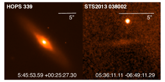
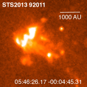
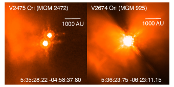
Appendix F The Effect of the Adopted Dust Law on Cavity Morphology

In our modeling, we used the dust opacity models adopted by (Furlan et al., 2016). To investigate the role of the assumed dust law on the observed morphology, we compared images generated with two dust opacity models from Ormel et al. (2011). The opacity model used in this paper, "icsgra3," is described in Section 3 and adopts a grain coagulation time of 0.3 Myr. We compare this to the opacity model "icsgra2" which in contrasts adopts a time of 0.1 Myr with consequently more grains of smaller sizes. When comparing model protostars from our grid generated with otherwise identical parameters, we observe that those using "icsgra2" show strongly limb brightened cavity edge profiles and bright point sources (Figure 40). In contrast, the larger grains present in "icsgra3" result in more forward scattering where the intensity peaks toward the center of the cavity instead of the edges. The "icsgra3" are more consistent with HST observations which typically show the cavities filled with emission (Figure 5), although there are some examples that show enhanced edges (Figure 13). This suggests that the larger grains in "icsgra3" are more representative of our sample (Appendix A). Although beyond the scope of this investigation, future studies of the observed cavity morphologies may provide new constraints on grain properties and their variations.

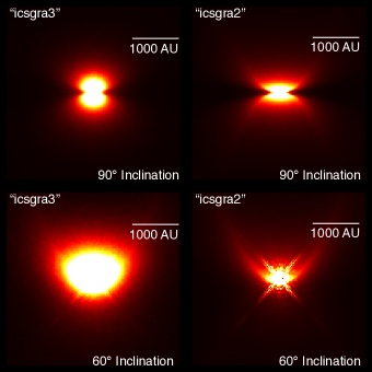
Appendix G Comparison Between SED Modeling and Near-IR Morphologies

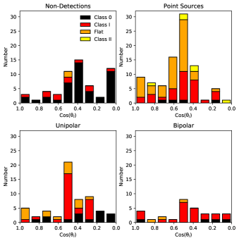
Most of the protostars in this paper have been characterized in detail by Furlan et al. (2016) using modeling in concert with the SEDs of these objects. The models used by these authors differ from those discussed in Section 3, and are fit to the SED from $1.6870\text{\,}\mathrm{\SIUnitSymbolMicro m}$ . The primarily differences that affect the $1.60\text{\,}\mathrm{\SIUnitSymbolMicro m}$ emission are that our grid uses a finer sampling of high inclination protostars, a sparser grid of envelope densities, and a different cavity opening angle exponent (2 vs 1.5).

Figure 41 shows histograms of the number of protostars vs inclinations determined by SED fitting. Four different histograms are displayed, one each for bipolar, unipolar, point sources, and non-detections. (Irregular protostars are not shown). Since the bins are chosen to have equal intervals in the cosine of the inclination, a random distribution should result in an equal number of sources in each bin; however, the SED-determined inclination for the overall sample of HOPS protostars peak at $6070\text{\,}\mathrm{\SIUnitSymbolDegree}$ , suggesting that the SED derived inclinations may have systematic biases (Furlan et al., 2016). The distribution of inclinations for point sources is similar in this respect to the overall sample (see Furlan et al., 2016, Figure 29), except at the highest inclinations. Obscuration by the disk likely accounts for this deficiency, both by decreasing the ability to detect a point source and by decreasing the contrast with the surrounding nebulosity. The unipolar and non-detections also peak around $6070\text{\,}\mathrm{\SIUnitSymbolDegree}$ , although they show a deficiency of low inclination objects, this is expected since the outflow cavities cannot be detected at low inclinations the lower obscuration at these angles makes non-detections unlikely.

Finally, the bipolar protostars show a broad range of inclinations, even though their observed morphologies require a nearly edge-on perspective. Furlan et al. (2016) showed that there are large systematic uncertainties in the SED derived inclinations. This figure further demonstrates the limitations of using SED derived inclinations, particularly for edge-on protostars. In a detailed study of the HST morphology of the HOPS 136 protostar, Fischer et al. (2014) could only find agreement between the SED models and the edge-on morphology by adding a low density component of dust in the outflow cavity to increase the scattering at shorter wavelengths. This suggests that our models are incomplete and therefore under-predict the brightness of protostars in the near-IR; consequently, model fits erroneously favor inclined models where the near-IR emission is less absorbed by the disk.

Our measurements of the cavity half-opening angles can also be used to test the angles derived from SED models. Furlan et al. (2016) fitted models with discrete cavity half-opening angles of $515253545\text{\,}\mathrm{\SIUnitSymbolDegree}$ for cavities with a $r^{1.5}$ power-law shape.¹³¹³13Note that they use the terminology “cavity opening angle” where we use “cavity half-opening angle”. The consistency of the best fit cavity angle compared to the mode for various criteria of close models are shown in Figure 46 of that work; This is further demonstrated in Figure 42, where we compare half-opening angles inferred from the best SED fits from Furlan et al. (2016) to the cavity half-opening angles derived in this work. In spite of the different cavity shapes assumed, a monotonically increasing correlation should be seen if both are accurate measurements of the cavity size. Since we do not see the expected correlation, and since most protostars have decent quality model fits for a range of cavity angles in the SED model grid, we find the cavity opening angles are not well constrained by SED modeling. A similar result was found by Seale & Looney (2008).