Abstract

Random Reshuffling (RR), also known as Stochastic Gradient Descent (SGD) without replacement, is a popular and theoretically grounded method for finite-sum minimization. We propose two new algorithms: Proximal and Federated Random Reshuffing (ProxRR and FedRR). The first algorithm, ProxRR, solves composite convex finite-sum minimization problems in which the objective is the sum of a (potentially non-smooth) convex regularizer and an average of $n$ smooth objectives. We obtain the second algorithm, FedRR, as a special case of ProxRR applied to a reformulation of distributed problems with either homogeneous or heterogeneous data. We study the algorithms’ convergence properties with constant and decreasing stepsizes, and show that they have considerable advantages over Proximal and Local SGD. In particular, our methods have superior complexities and ProxRR evaluates the proximal operator once per epoch only. When the proximal operator is expensive to compute, this small difference makes ProxRR up to $n$ times faster than algorithms that evaluate the proximal operator in every iteration. We give examples of practical optimization tasks where the proximal operator is difficult to compute and ProxRR has a clear advantage. Finally, we corroborate our results with experiments on real data sets.

1 Introduction

Modern theory and practice of training supervised machine learning models is based on the paradigm of regularized empirical risk minimization (ERM) (Shalev-Shwartz & Ben-David, 2014). While the ultimate goal of supervised learning is to train models that generalize well to unseen data, in practice only a finite data set is available during training. Settling for a model merely minimizing the average loss on this training set—the empirical risk—is insufficient, as this often leads to over-fitting and poor generalization performance in practice. Due to this reason, empirical risk is virtually always amended with a suitably chosen regularizer whose role is to encode prior knowledge about the learning task at hand, thus biasing the training algorithm towards better performing models.

The regularization framework is quite general and perhaps surprisingly it also allows us to consider methods for federated learning (FL)—a paradigm in which we aim at training model for a number of clients that do not want to reveal their data (Konečný et al., 2016; McMahan et al., 2017; Kairouz, 2019). The training in FL usually happens on devices with only a small number of model updates being shared with a global host. To this end, Federated Averaging algorithm has emerged that performs Local SGD updates on the clients’ devices and periodically aggregates their average. Its analysis usually requires special techniques and deliberately constructed sequences hindering the research in this direction. We shall see, however, that the convergence of our FedRR follows from merely applying our algorithm for regularized problems to a carefully chosen reformulation.

Formally, regularized ERM problems are optimization problems of the form

$$\textstyle\min\limits_{x\in\mathbb{R}^{d}}\Bigl{[}P(x)\overset{\text{def}}{=}\frac{1}{n}\sum\limits_{i=1}^{n}f_{i}(x)+\psi(x)\Bigr{]},$$ (1)

where $f_{i}:\mathbb{R}^{d}\to\mathbb{R}$ is the loss of model parameterized by vector $x\in\mathbb{R}^{d}$ on the $i$-th training data point, and $\psi:\mathbb{R}^{d}\to\mathbb{R}\cup\{+\infty\}$ is a regularizer. Let $[n]\overset{\text{def}}{=}\{1,2,\dots,n\}$. We shall make the following assumption throughout the paper without explicitly mentioning it:

Assumption 1.

The functions $f_{i}$ are $L_{i}$-smooth and convex, and the regularizer $\psi$ is proper, closed and convex. Let $L_{\max}\overset{\text{def}}{=}\max_{i\in[n]}L_{i}$.

In some results we will additionally assume that either the individual functions $f_{i}$, or their average $f\overset{\text{def}}{=}\frac{1}{n}\sum_{i}f_{i}$, or the regularizer $\psi$ are $\mu$-strongly convex. Whenever we need such additional assumptions, we will make this explicitly clear. While all these concepts are standard, we review them briefly in Section 9.

Proximal SGD. When the number $n$ of training data points is huge, as is increasingly common in practice, the most efficient algorithms for solving (1) are stochastic first-order methods, such as stochastic gradient descent (SGD) (Bordes et al., 2009), in one or another of its many variants proposed in the last decade (Shang et al., 2018; Pham et al., 2020). These method almost invariably rely on alternating stochastic gradient steps with the evaluation of the proximal operator

$$\textstyle\mathrm{prox}_{\gamma\psi}(x)\overset{\text{def}}{=}\operatorname*{\arg\!\min}_{z\in\mathbb{R}^{d}}\left\{\gamma\psi(z)+\frac{1}{2}\|z-x\|^{2}\right\}.$$

The simplest of these has the form

$$x_{k+1}^{\mathrm{SGD}}=\mathrm{prox}_{\gamma_{k}\psi}(x_{k}^{\mathrm{SGD}}-\gamma_{k}\nabla f_{i_{k}}(x_{k}^{\mathrm{SGD}})),$$ (2)

where $i_{k}$ is an index from $\{1,2,\dots,n\}$ chosen uniformly at random, and $\gamma_{k}>0$ is a properly chosen learning rate. Our understanding of (2) is quite mature; see (Gorbunov et al., 2020) for a general treatment which considers methods of this form in conjunction with more advanced stochastic gradient estimators in place of $\nabla f_{i_{k}}$.

Applications such as training sparse linear models (Tibshirani, 1996), non-negative matrix factorization (Lee & Seung, 1999), image deblurring (Bredies et al., 2010), and training with group selection (Yuan & Lin, 2006) all rely on the use of hand-crafted regularizes. For most of them, the proximal operator can be evaluated efficiently, and SGD is near or at the top of the list of efficient training algorithms.

Random reshuffling. A particularly successful variant of SGD is based on the idea of random shuffling (permutation) of the training data followed by $n$ iterations of the form (2), with the index $i_{k}$ following the pre-selected permutation (Bottou, 2012). This process is repeated several times, each time using a new freshly sampled random permutation of the data, and the resulting method is known under the name Random Reshuffling (RR). When the same permutation is used throughout, the technique is known under the name Shuffle Once (SO).

One of the main advantages of this approach is rooted in its intrinsic ability to avoid cache misses when reading the data from memory, which enables a significantly faster implementation. Furthermore, RR is often observed to converge in fewer iterations than SGD in practice. This can intuitively be ascribed to the fact that while due to its sampling-with-replacement approach SGD can miss to learn from some data points in any given epoch, RR will necessarily learn from each data point in each epoch.

Understanding the random reshuffling trick, and why it works, has been a non-trivial open problem for a long time (Bottou, 2009; Recht & Ré, 2012; Gürbüzbalaban et al., 2019; Haochen & Sra, 2019). Until recent development which lead to a significant simplification of the convergence analysis technique and proofs (Mishchenko et al., 2020), prior state of the art relied on long and elaborate proofs requiring sophisticated arguments and tools, such as analysis via the Wasserstein distance (Nagaraj et al., 2019), and relied on a significant number of strong assumptions about the objective (Shamir, 2016; Haochen & Sra, 2019). In alternative recent development, Ahn et al. (2020) also develop new tools for analyzing the convergence of random reshuffling, in particular using decreasing stepsizes and for objectives satisfying the Polyak-Łojasiewicz condition, a generalization of strong convexity (Polyak, 1963; Lojasiewicz, 1963).

The difficulty of analyzing RR has been the main obstacle in the development of even some of the most seemingly benign extensions of the method. Indeed, while all these are well understood in combination with its much simpler-to-analyze cousin SGD, to the best of our knowledge, there exists no theoretical analysis of proximal, parallel, and importance sampling variants of RR with both constant and decreasing stepsizes, and in most cases it is not even clear how should such methods be constructed. Empowered by and building on the recent advances of Mishchenko et al. (2020), in this paper we address all these challenges.

2 Contributions

In this section we outline the key contributions of our work, and also offer a few intuitive explanations motivating some of the development.

From RR to proximal RR. Despite rich literature on proximal SGD (Gorbunov et al., 2020), it is not obvious how one should extend RR to solve problem (1) when a nonzero regularizer $\psi$ is present. Indeed, the standard practice for SGD is to apply the proximal operator after each stochastic step (Duchi & Singer, 2009), i.e., in analogy with (2). On the other hand, RR is motivated by the fact that a data pass approximates the full gradient step. If we apply the proximal operator after each iteration of RR, we would no longer approximate the full gradient after an epoch, as illustrated by the next example.

Example 1.

Let $n=2$, $\psi(x)=\frac{1}{2}\|x\|^{2}$, $f_{1}(x)=\langle c_{1},x\rangle$, $f_{2}(x)=\langle c_{2},x\rangle$ with some $c_{1},c_{2}\in\mathbb{R}^{d}$, $c_{1}\neq c_{2}$. Let $x_{0}\in\mathbb{R}^{d}$, $\gamma>0$ and define $x_{1}=x_{0}-\gamma\nabla f_{1}(x_{0})$, $x_{2}=x_{1}-\gamma\nabla f_{2}(x_{1})$. Then, we have $\mathrm{prox}_{2\gamma\psi}(x_{2})=\mathrm{prox}_{2\gamma\psi}(x_{0}-2\gamma\nabla f(x_{0}))$. However, if $\tilde{x}_{1}=\mathrm{prox}_{\gamma\psi}(x_{0}-\gamma\nabla f_{1}(x_{0}))$ and $\tilde{x}_{2}=\mathrm{prox}_{\gamma\psi}(x_{1}-\gamma\nabla f_{2}(\tilde{x}_{1}))$, then $\tilde{x}_{2}\neq\mathrm{prox}_{2\gamma\psi}(x_{0}-2\gamma\nabla f(x_{0}))$.

Motivated by this observation, we propose ProxRR (Algorithm 1), in which the proximal operator is applied at the end of each epoch of RR, i.e., after each pass through all randomly reshuffled data.

Algorithm 1 Proximal Random Reshuffling (ProxRR) and Shuffle-Once (ProxSO)

1:Stepsizes $\gamma_{t}>0$, initial vector $x_{0}\in\mathbb{R}^{d}$, number of epochs $T$

2:Sample a permutation $\pi=(\pi_{0},\pi_{1},\ldots,\pi_{n-1})$ of $[n]$ (Do step 1 only for ProxSO)

3:for epochs $t=0,1,\dotsc,T-1$ do

4:     Sample a permut. $\pi=(\pi_{0},\pi_{1},\ldots,\pi_{n-1})$ of $[n]$ (Do step 3 only for ProxRR)

5:     $x_{t}^{0}=x_{t}$

6:     for $i=0,1,\ldots,n-1$ do

7:         $x_{t}^{i+1}=x_{t}^{i}-\gamma_{t}\nabla f_{\pi_{i}}(x_{t}^{i})$      

8:     $x_{t+1}=\mathrm{prox}_{\gamma_{t}n\psi}(x_{t}^{n})$

A notable property of Algorithm 1 is that only a single proximal operator evaluation is needed during each data pass. This is in sharp contrast with the way proximal SGD works, and offers significant advantages in regimes where the evaluation of the proximal mapping is expensive (e.g., comparable to the evaluation of $n$ gradients $\nabla f_{1},\dots,\nabla f_{n}$).

We establish several convergence results for ProxRR, of which we highlight two here. Both offer a linear convergence rate with a fixed stepsize to a neighborhood of the solution. Firstly, in the case when each $f_{i}$ is $\mu$-strongly convex, we prove the rate (see Theorem 2)

$$\textstyle\mathbb{E}\left[\left\lVert x_{T}-x_{\ast}\right\rVert^{2}\right]\leq\left(1-\gamma\mu\right)^{nT}{\left\lVert x_{0}-x_{\ast}\right\rVert}^{2}+\frac{2\gamma^{2}\sigma_{\mathrm{rad}}^{2}}{\mu},$$

where $\gamma_{t}=\gamma\leq\frac{1}{L_{\max}}$ is the stepsize, and $\sigma_{\mathrm{rad}}^{2}$ is a shuffling radius constant (for precise definition, see (4)). In Theorem 1 we bound the shuffling radius in terms of $\left\lVert\nabla f(x_{\ast})\right\rVert^{2}$, $n$, $L_{\max}$ and the more common quantity $\sigma_{\ast}^{2}\overset{\text{def}}{=}\frac{1}{n}\sum_{i=1}^{n}{\left\lVert\nabla f_{i}(x_{\ast})-\nabla f(x_{\ast})\right\rVert}^{2}$.

Secondly, if $\psi$ is $\mu$-strongly convex, we prove the rate

$$\textstyle\mathbb{E}\left[\left\lVert x_{T}-x_{\ast}\right\rVert^{2}\right]\leq\left(1+2\gamma\mu n\right)^{-T}{\left\lVert x_{0}-x_{\ast}\right\rVert}^{2}+\frac{\gamma^{2}\sigma_{\mathrm{rad}}^{2}}{\mu},$$

where $\gamma_{t}=\gamma\leq\frac{1}{L_{\max}}$ is the stepsize (see Theorem 4) .

Both mentioned rates show exponential (linear in logarithmic scale) convergence to a neighborhood whose size is proportional to $\gamma^{2}\sigma_{\mathrm{rad}}^{2}$. Since we can choose $\gamma$ to be arbitrarily small or periodically decrease it, this implies that the iterates converge to $x_{\ast}$ in the limit. Moreover, we show in Section 4 that when $\gamma=\mathcal{O}(\frac{1}{T})$ the error is $\mathcal{O}(\frac{1}{T^{2}})$, which is superior to the $\mathcal{O}(\frac{1}{T})$ error of SGD.

Decreasing stepsizes. The convergence of RR is not always exact and depends on the parameters of the objective. Similarly, if the shuffling radius $\sigma_{\mathrm{rad}}^{2}$ is positive, and we wish to find an $\varepsilon$-approximate solution, the optimal choice of a fixed stepsize for ProxRR will depend on $\varepsilon$. This deficiency can be fixed by using decreasing stepsizes in both vanilla RR (Ahn et al., 2020) and in SGD (Stich, 2019). We adopt the same technique to our setting. However, we depart from (Ahn et al., 2020) by only adjusting the stepsize once per epoch rather than at every iteration, similarly to the concurrent work of Tran et al. (2020) on RR with momentum. For details, see Section 6.

Importance sampling for proximal RR. While importance sampling is a well established technique for speeding up the convergence of SGD (Zhao & Zhang, 2015; Khaled & Richtárik, 2020), no importance sampling variant of RR has been proposed nor analyzed. This is not surprising since the key property of importance sampling in SGD—unbiasedness—does not hold for RR. Our approach to equip ProxRR with importance sampling is via a reformulation of problem (1) into a similar problem with a larger number of summands. In particular, for each $i\in[n]$ we include $n_{i}$ copies of the function $\frac{1}{n_{i}}f_{i}$, and then take average of all $N=\sum_{i}n_{i}$ functions constructed this way. The value of $n_{i}$ depends on the “importance” of $f_{i}$, described below. We then apply ProxRR to this reformulation.

If $f_{i}$ is $L_{i}$-smooth for all $i\in[n]$ and we let $\bar{L}\overset{\text{def}}{=}\frac{1}{n}\sum_{i}L_{i}$, then we choose $n_{i}=\lceil\frac{L_{i}}{\bar{L}}\rceil$. It is easy to show that $N\leq 2n$, and hence our reformulation leads to at most a doubling of the number of functions forming the finite sum. However, the overall complexity of ProxRR applied to this reformulation will depend on $\bar{L}$ instead of $\max_{i}L_{i}$ (see Theorem 6), which can lead to a significant improvement. For details of the construction and our complexity results, see Section 6.

Application to Federated Learning. In Section 7 we describe an application of our results to federated learning (Konečný et al., 2016; McMahan et al., 2017; Kairouz, 2019).

Results for SO. All of our results apply to the Shuffle-Once algorithm as well. For simplicity, we center the discussion around RR, whose current theoretical guarantees in the non-convex case are better than that of SO. Nevertheless, the other results are the same for both methods, and ProxRR is identical to ProxSO in terms of our theory too. A study of the empirical differences between RR and SO can be found in (Mishchenko et al., 2020).

3 Preliminaries

In our analysis, we build upon the notions of limit points and shuffling variance introduced by Mishchenko et al. (2020) for vanilla (i.e., non-proximal) RR. Given a stepsize $\gamma>0$ (held constant during each epoch) and a permutation $\pi$ of $\{1,2,\dots,n\}$, the inner loop iterates of RR/SO converge to a neighborhood of intermediate limit points $x_{\ast}^{1},x_{\ast}^{2},\ldots,x_{\ast}^{n}$ defined by

$$\textstyle x_{\ast}^{i}\overset{\text{def}}{=}x_{\ast}-\gamma\sum\limits_{j=0}^{i-1}\nabla f_{\pi_{j}}(x_{\ast}),\quad i=1,\dotsc,n-1.$$ (3)

The intuition behind this definition is fairly simple: if we performed $i$ steps starting at $x_{*}$, we would end up close to $x_{*}^{i}$. To quantify the closeness, we define the shuffling radius.

Definition 1 (Shuffling radius).

Given a stepsize $\gamma>0$ and a random permutation $\pi$ of $\{1,2,\ldots,n\}$ used in Algorithm 1, define $x_{\ast}^{i}=x_{\ast}^{i}(\gamma,\pi)$ as in (3). Then, the shuffling radius is defined by

$$\textstyle\sigma_{\mathrm{rad}}^{2}(\gamma)\overset{\text{def}}{=}\max\limits_{i=1,\ldots,n-1}\left[\frac{1}{\gamma^{2}}\mathbb{E}_{\pi}\bigl{[}D_{f_{\pi_{i}}}(x_{\ast}^{i},x_{\ast})\bigr{]}\right],$$ (4)

where the expectation is taken with respect to the randomness in the permutation $\pi$. If there are multiple stepsizes $\gamma_{1},\gamma_{2},\ldots$ used in Algorithm 1, we take the maximum of all of them as the shuffling radius, i.e.,

$$\sigma_{\mathrm{rad}}^{2}\overset{\text{def}}{=}\smash{\max_{t=1,2\dotsc}}\sigma_{\mathrm{rad}}^{2}(\gamma_{t}).$$

The shuffling radius is related by a multiplicative factor in the stepsize to the shuffling variance introduced by Mishchenko et al. (2020). When the stepsize is held fixed, the difference between the two notions is minimal but when the stepsize is decreasing, the shuffling radius is easier to work with, since it can be upper bounded by problem constants independent of the stepsizes. To prove this upper bound, we rely on a lemma due to Mishchenko et al. (2020) that bounds the variance when sampling without replacement.

Lemma 1 (Lemma 1 in (Mishchenko et al., 2020)).

Let $X_{1},\ldots,X_{n}\in\mathbb{R}^{d}$ be fixed vectors, let $\bar{X}=\frac{1}{n}\sum_{i=1}^{n}X_{i}$ be their mean, and let $\sigma^{2}=\frac{1}{n}\sum_{i=1}^{n}{\left\lVert X_{i}-\bar{X}\right\rVert}^{2}$ be their variance. Fix any $i\in\{1,\ldots,n\}$ and let $X_{\pi_{0}},\ldots,X_{\pi_{i-1}}$ be sampled uniformly without replacement from $\{X_{1},\ldots,X_{n}\}$ and $\bar{X}_{\pi}=\frac{1}{i}\sum_{j=0}^{i-1}X_{\pi_{j}}$ be their average. Then, the sample average and variance are given by

$$\textstyle\mathbb{E}\left[\bar{X}_{\pi}\right]=\bar{X},\qquad\mathbb{E}\left[\left\lVert\bar{X}_{\pi}-\bar{X}\right\rVert^{2}\right]=\frac{n-i}{i(n-1)}\sigma^{2}.$$ (5)

Armed with Lemma 1, we can upper bound the shuffling radius using the smoothness constant $L_{\max}$, size of the vector $\nabla f(x_{\ast})$ and the variance $\sigma_{\ast}^{2}$ of the gradient vectors $\nabla f_{1}(x_{\ast})$, $\nabla f_{2}(x_{\ast})$, …, $\nabla f_{n}(x_{\ast})$.

Theorem 1.

For any stepsize $\gamma>0$ and any random permutation $\pi$ of $\{1,2,\dots,n\}$ we have

$$\textstyle\sigma_{\mathrm{rad}}^{2}\leq\frac{L_{\max}}{2}n\Bigl{(}n\|\nabla f(x_{\ast})\|^{2}+\frac{1}{2}\sigma_{\ast}^{2}\Bigr{)},$$

where $x_{\ast}$ is a solution of Problem (1) and $\sigma_{\ast}^{2}$ is the population variance at the optimum

$$\textstyle\sigma_{\ast}^{2}\overset{\text{def}}{=}\frac{1}{n}\smash{\sum\limits_{i=1}^{n}}{\left\lVert\nabla f_{i}(x_{\ast})-\nabla f(x_{\ast})\right\rVert}^{2}.$$ (6)

All proofs are relegated to the supplementary material. In order to better understand the bound given by Theorem 1, note that if there is no proximal operator (i.e., $\psi=0$) then $\nabla f(x_{\ast})=0$ and we get that $\sigma_{\mathrm{rad}}^{2}\leq\frac{L_{\max}n\sigma_{\ast}^{2}}{4}$. This recovers the existing upper bound on the shuffling variance of Mishchenko et al. (2020) for vanilla RR. On the other hand, if $\nabla f(x_{\ast})\neq 0$ then we get an additive term of size proportional to the squared norm of $\nabla f(x_{\ast})$.

4 Theory for strongly convex losses $f_{1},\dots,f_{n}$

Our first theorem establishes a convergence rate for Algorithm 1 applied with a constant stepsize to Problem (1) when each objective $f_{i}$ is strongly convex. This assumption is commonly satisfied in machine learning applications where each $f_{i}$ represents a regularized loss on some data points, as in $\ell_{2}$ regularized linear regression and $\ell_{2}$ regularized logistic regression.

Theorem 2.

Let Assumption 1 be satisfied. Further, assume that each $f_{i}$ is $\mu$-strongly convex. If Algorithm 1 is run with constant stepsize $\gamma_{t}=\gamma\leq\frac{1}{L_{\max}}$, then the iterates generated by the algorithm satisfy

$$\textstyle\mathbb{E}\left[\left\lVert x_{T}-x_{\ast}\right\rVert^{2}\right]\leq\left(1-\gamma\mu\right)^{nT}{\left\lVert x_{0}-x_{\ast}\right\rVert}^{2}+\frac{2\gamma^{2}\sigma_{\mathrm{rad}}^{2}}{\mu}.$$

We can convert the guarantee of Theorem 2 to a convergence rate by properly tuning the stepsize and using the upper bound of Theorem 1 on the shuffling radius. In particular, if we choose the stepsize as $\gamma=\min\left\{\frac{1}{L_{\max}},\frac{\sqrt{\varepsilon\mu}}{\sqrt{2}\sigma_{\mathrm{rad}}}\right\},$ then we obtain $\mathbb{E}\left[\left\lVert x_{T}-x_{\ast}\right\rVert^{2}\right]=\mathcal{O}\left(\varepsilon\right)$ provided that the total number of iterations $K_{\mathrm{RR}}=nT$ is at least

$$\textstyle K_{\mathrm{RR}}\geq\biggl{(}\kappa+\frac{\sqrt{\kappa n}}{\sqrt{\varepsilon}\mu}(\sqrt{n}\left\lVert\nabla f(x_{\ast})\right\rVert+\sigma_{\ast})\biggr{)}\log\left(\frac{2r_{0}}{\varepsilon}\right),$$ (7)

where $\kappa\overset{\text{def}}{=}L_{\max}/\mu$ and $r_{0}\overset{\text{def}}{=}\|x_{0}-x_{\ast}\|^{2}$.

Comparison with vanilla RR. If there is no proximal operator, then $\left\lVert\nabla f(x_{\ast})\right\rVert=0$ and we recover the earlier result of Mishchenko et al. (2020) on the convergence of RR without proximal, which is optimal in $\varepsilon$ up to logarithmic factors. On the other hand, when the proximal operator is nonzero, we get an extra term in the complexity proportional to $\left\lVert\nabla f(x_{\ast})\right\rVert$: thus, even when all the functions are the same (i.e., $\sigma_{\ast}=0$), we do not recover the linear convergence of Proximal Gradient Descent (Karimi et al., 2016; Beck, 2017). This can be easily explained by the fact that Algorithm 1 performs $n$ gradient steps per one proximal step. Hence, even if $f_{1}=\dotsb=f_{n}$, Algorithm 1 does not reduce to Proximal Gradient Descent. We note that other algorithms for composite optimization which may not take a proximal step at every iteration (for example, using stochastic projection steps) also suffer from the same dependence (Patrascu & Irofti, 2020).

Comparison with proximal SGD. In order to compare (7) against the complexity of Proximal SGD (Algorithm 2), we recall the following simple result on the convergence of Proximal SGD. The result is standard Needell et al. (2016); Gower et al. (2019), with the exception that we present it in a slightly generalized in that we also consider the case when $\psi$ is strongly convex. Our proof is a minor modification of that in Gower et al. (2019), and we offer it in the appendix for completeness.

Algorithm 2 Proximal SGD

1:Stepsizes $\gamma_{k}>0$, initial vector $x_{0}\in\mathbb{R}^{d}$, number of steps $K$

2:for steps $k=0,1,\dotsc,K-1$ do

3:     Sample $i_{k}$ uniformly at random from $[n]$

4:     $x_{k+1}=\mathrm{prox}_{\gamma_{k}\psi}(x_{k}-\gamma_{k}\nabla f_{i_{k}}(x_{k}))$

Theorem 3 (Proximal SGD).

Let Assumption 1 hold. Further, suppose that either $f\overset{\text{def}}{=}\frac{1}{n}\sum_{i=1}^{n}f_{i}$ is $\mu$-strongly convex or that $\psi$ is $\mu$-strongly convex. If Algorithm 2 is run with a constant stepsize $\gamma_{k}=\gamma>0$ satisfying $\gamma\leq\frac{1}{2L_{\max}}$, then the final iterate returned by the algorithm after $K$ steps satisfies

$$\textstyle\mathbb{E}\left[\left\lVert x_{K}-x_{\ast}\right\rVert^{2}\right]\leq\left(1-\gamma\mu\right)^{K}{\left\lVert x_{0}-x_{\ast}\right\rVert}^{2}+\frac{2\gamma\sigma_{\ast}^{2}}{\mu}.$$

Furthermore, by choosing the stepsize $\gamma$ as $\gamma=\min\left\{\frac{1}{2L_{\max}},\frac{\varepsilon\mu}{4\sigma_{\ast}}\right\}$, we get that $\mathbb{E}\left[\left\lVert x_{K}-x_{\ast}\right\rVert^{2}\right]=\mathcal{O}\left(\varepsilon\right)$ provided that the number of iterations is at least

$$\textstyle K_{\mathrm{SGD}}\geq\left(\kappa+\frac{\sigma_{\ast}^{2}}{\varepsilon\mu^{2}}\right)\log\left(\frac{2r_{0}}{\varepsilon}\right).$$ (8)

By comparing between the iteration complexities $K_{\mathrm{SGD}}$ (given by (8)) and $K_{\mathrm{RR}}$ (given by (7)), we see that ProxRR converges faster than Proximal SGD whenever the target accuracy $\varepsilon$ is small enough to satisfy

$$\textstyle\varepsilon\leq\frac{1}{L_{\max}n\mu}\left(\frac{\sigma_{\ast}^{4}}{n{\left\lVert\nabla f(x_{\ast})\right\rVert}^{2}+\sigma_{\ast}^{2}}\right).$$

Furthermore, the comparison is much better when we consider proximal iteration complexity (number of proximal operator access), in which case the complexity of ProxRR (7) is reduced by a factor of $n$ (because we take one proximal step every $n$ iterations) while the proximal iteration complexity of Proximal SGD remains the same as (8). In this case, ProxRR is better whenever the accuracy $\varepsilon$ satisfies

$$\begin{split}\varepsilon&\textstyle\geq\frac{n}{L_{\max}\mu}\left[n{\left\lVert\nabla f(x_{\ast})\right\rVert}^{2}+\sigma_{\ast}^{2}\right]\\ \qquad\text{or},\qquad\varepsilon&\textstyle\leq\frac{n}{L_{\max}\mu}\left[\frac{\sigma_{\ast}^{4}}{n{\left\lVert\nabla f(x_{\ast})\right\rVert}^{2}+\sigma_{\ast}^{2}}\right].\end{split}$$

Therefore we can see that if the target accuracy is large enough or small enough, and if the cost of proximal operators dominates the computation, ProxRR is much quicker to converge than Proximal SGD.

5 Theory for strongly convex regularizer $\psi$

In Theorem 2, we assume that each $f_{i}$ is $\mu$-strongly convex. This is motivated by the common practice of using $\ell_{2}$ regularization in machine learning. However, applying $\ell_{2}$ regularization in every step of Algorithm 1 can be expensive when the data are sparse and the iterates $x_{t}^{i}$ are dense, because it requires accessing each coordinate of $x_{t}^{i}$ which can be much more expensive than computing sparse gradients $\nabla f_{i}(x_{t}^{i})$. Alternatively, we may instead choose to put the $\ell_{2}$ regularization inside $\psi$ and only ask that $\psi$ be strongly convex—this way, we can save a lot of time as we need to access each coordinate of the dense iterates $x_{t}^{i}$ only once per epoch rather than every iteration. Theorem 4 gives a convergence guarantee in this setting.

Theorem 4.

Let Assumption 1 be satisfied. Further, assume that $\psi$ is $\mu$-strongly convex. If Algorithm 1 is run with constant stepsize $\gamma_{t}=\gamma\leq\frac{1}{L_{\max}}$, where $L_{\max}=\max_{i}L_{i}$, then the iterates generated by the algorithm satisfy

$$\textstyle\mathbb{E}\left[\left\lVert x_{T}-x_{\ast}\right\rVert^{2}\right]\leq\left(1+2\gamma\mu n\right)^{-T}{\left\lVert x_{0}-x_{\ast}\right\rVert}^{2}+\frac{\gamma^{2}\sigma_{\mathrm{rad}}^{2}}{\mu}.$$

By making a specific choice for the stepsize used by Algorithm 1, we can obtain a convergence guarantee using Theorem 4. Choosing the stepsize as

$$\textstyle\gamma=\min\left\{\frac{1}{L_{\max}},\frac{\sqrt{\varepsilon\mu}}{\sigma_{\mathrm{rad}}}\right\}.$$ (9)

Then $\mathbb{E}\left[\left\lVert x_{T}-x_{\ast}\right\rVert^{2}\right]=\mathcal{O}\left(\varepsilon\right)$ provided that the total number of iterations satisfies

$$\textstyle K\geq\left(\kappa+\frac{\sigma_{\mathrm{rad}}/\mu}{\sqrt{\varepsilon\mu}}+n\right)\log\left(\frac{2r_{0}}{\varepsilon}\right).$$ (10)

This can be converted to a bound similar to (7) by using Theorem 1, in which case the only difference between the two cases is an extra $n\log\left(\frac{1}{\varepsilon}\right)$ term when only the regularizer $\psi$ is $\mu$-strongly convex. Since for small enough accuracies the $1/\sqrt{\varepsilon}$ term dominates, this difference is minimal.

6 Extensions

Before turning to applications, we discuss two extensions to the theory that significantly matter in practice: using decreasing stepsizes and applying importance resampling.

Decreasing stepsizes. Using the theoretical stepsize (9) requires knowing the desired accuracy $\varepsilon$ ahead of time as well as estimating $\sigma_{\mathrm{rad}}$. It also results in extra polylogarithmic factors in the iteration complexity (10), a phenomenon observed and fixed by using decreasing stepsizes in both vanilla RR (Ahn et al., 2020) and in SGD (Stich, 2019). We show that we can adopt the same technique to our setting. However, we depart from the stepsize scheme of Ahn et al. (2020) by only varying the stepsize once per epoch rather than every iteration. This is closer to the common practical heuristic of decreasing the stepsize once every epoch or once every few epochs (Sun, 2020; Tran et al., 2020). The stepsize scheme we use is inspired by the schemes of (Stich, 2019; Khaled & Richtárik, 2020): in particular, we fix $T>0$, let $t_{0}=\lceil T/2\rceil$, and choose the stepsizes $\gamma_{t}>0$ by

$$\gamma_{t}=\begin{cases}\frac{1}{L_{\max}}&\text{ if }T\leq\frac{L_{\max}}{2\mu n}\text{ or }t\leq t_{0},\\ \frac{7}{\mu n\left(s+t-t_{0}\right)}&\text{ if }T>\frac{L_{\max}}{2\mu n}\text{ and }t>t_{0},\end{cases}$$ (11)

where $s\overset{\text{def}}{=}7L_{\max}/(4\mu n)$. Hence, we fix the stepsize used in the first $T/2$ iterations and then start decreasing it every epoch afterwards. Using this stepsize schedule, we can obtain the following convergence guarantee when each $f_{i}$ is smooth and convex and the regularizer $\psi$ is $\mu$-strongly convex.

Theorem 5.

Suppose that each $f_{i}$ is $L_{\max}$-smooth and convex, and that the regularizer $\psi$ is $\mu$-strongly convex. Fix $T>0$. Then choosing stepsizes $\gamma_{t}$ according to (11) we have that $\gamma_{t}\leq\frac{1}{L_{\max}}$ for all $t$ and the final iterate generated by Algorithm 1 satisfies

$$\textstyle\mathbb{E}\left[\left\lVert x_{T}-x_{\ast}\right\rVert^{2}\right]=\mathcal{O}\left(\exp\left(-\frac{nT}{\kappa+2n}\right)r_{0}+\frac{\sigma_{\mathrm{rad}}^{2}}{\mu^{3}n^{2}T^{2}}\right),$$

where $\kappa\overset{\text{def}}{=}L_{\max}/\mu$, $r_{0}\overset{\text{def}}{=}\|x_{0}-x_{\ast}\|^{2}$ and $\mathcal{O}(\cdot)$ hides absolute (non-problem-specific) constants.

This guarantee holds for any number of epochs $T>0$. We believe a similar guarantee can be obtained in the case each $f_{i}$ is strongly-convex and the regularizer $\psi$ is just convex, but we did not include it as it adds little to the overall message.

Importance resampling. Suppose that each $f_{i}$ is $L_{i}$-smooth. Then the iteration complexities of both SGD and RR depend on $L_{\max}/\mu$, where $L_{\max}$ is the maximum smoothness constant among the smoothness constants $L_{1},L_{2},\ldots,L_{n}$. The maximum smoothness constant can be arbitrarily worse than the average smoothness constant $\bar{L}=\frac{1}{n}\sum_{i=1}^{n}L_{i}$. This situation is in contrast to the complexity of gradient descent which depends on the smoothness constant $L_{f}$ of $f=\frac{1}{n}\sum_{i=1}^{n}f_{i}$, for which we have $L_{f}\leq\bar{L}$. This is a problem commonly encountered with stochastic optimization methods and may cause significantly degraded performance in practical optimization tasks in comparison with deterministic methods (Tang et al., 2019).

Importance sampling is a common technique to improve the convergence of SGD (Algorithm 2): we sample function $\frac{\bar{L}}{L_{i}}f_{i}$ with probability $p_{i}$ proportional to $L_{i}$, where $\bar{L}\overset{\text{def}}{=}\frac{1}{n}\sum_{i=1}^{n}L_{i}$. In that case, the SGD update is still unbiased since

$$\textstyle\mathbb{E}_{i}\left[\frac{\bar{L}}{L_{i}}f_{i}\right]=\sum\limits_{i=1}^{n}p_{i}\frac{\bar{L}}{L_{i}}f_{i}=f.$$

Moreover, the smoothness of function $\frac{\bar{L}}{L_{i}}f_{i}$ is $\bar{L}$ for any $i$, so the guarantees would depend on $\bar{L}$ instead of $\max_{i=1,\dotsc,n}L_{i}$. Importance sampling successfully improves the iteration complexity of SGD to depend on $\bar{L}$ (Needell et al., 2016), and has been investigated in a wide variety of settings (Gower et al., 2020; Gorbunov et al., 2020).

Importance sampling is a neat technique but it relies heavily on the fact that we use unbiased sampling. How can we obtain a similar result if inside any permutation the sampling is biased? The answer requires us to think again as to what happens when we replace $f_{i}$ with $\frac{\bar{L}}{L_{i}}f_{i}$. To make sure the problem remains the same, it is sufficient to have $\frac{\bar{L}}{L_{i}}f_{i}$ inside a permutation exactly $\frac{L_{i}}{\bar{L}}$ times. And since $\frac{L_{i}}{\bar{L}}$ is not necessarily integer, we should use $n_{i}=\Bigl{\lceil}\frac{L_{i}}{\bar{L}}\Bigr{\rceil}$ and solve

$$\textstyle\min\limits_{x\in\mathbb{R}^{d}}\frac{1}{N}\sum\limits_{i=1}^{n}\Bigl{(}\underbrace{\tfrac{1}{n_{i}}f_{i}(x)+\dotsb+\tfrac{1}{n_{i}}f_{i}(x)}_{n_{i}\text{ times}}\Bigr{)}+\psi(x),$$ (12)

where $N\overset{\text{def}}{=}n_{1}+\dotsb+n_{n}=\Bigl{\lceil}\frac{L_{1}}{\bar{L}}\Bigr{\rceil}+\dotsb+\Bigl{\lceil}\frac{L_{n}}{\bar{L}}\Bigr{\rceil}$. Clearly, this problem is equivalent to the original formulation in 1. At the same time, we have improved all smoothness constants to $\bar{L}$. It might seem that that the new problem has more functions, but it turns out that the new number of functions satisfies $N\leq 2n$, so any related costs, such as longer loops or storing duplicates of the data, are negligible, as the next theorem shows.

Theorem 6.

For every $i$, assume that each $f_{i}$ is convex and $L_{i}$-smooth, and let $\psi$ be $\mu$-strongly convex. Then, the number of functions $N$ in (12) satisfies $N\leq 2n$, and Algorithm 1 applied to problem (12) has the same complexity as (10) but proportional to $\bar{L}$ rather than $L_{\max}$.

7 Federated learning

Let us consider now the problem of minimizing the average of $N=\sum_{m=1}^{M}N_{m}$ functions that are stored on $M$ devices, which have $N_{1},\dotsc,N_{M}$ samples correspondingly,

$$\textstyle\min\limits_{x\in\mathbb{R}^{d}}\frac{1}{N}\smash{\sum\limits_{m=1}^{M}}F_{m}(x)+R(x),\quad F_{m}(x)=\smash{\sum\limits_{j=1}^{N_{m}}}f_{mj}(x).$$

For example, $f_{mj}(x)$ can be the loss associated with a single sample $(X_{mj},y_{mj})$, where pairs $(X_{mj},y_{mj})$ follow a distribution $D_{m}$ that is specific to device $m$. An important instance of such formulation is federated learning, where $M$ devices train a shared model by communicating periodically with a server. We normalize the objective in (7) by $N$ as this is the total number of functions after we expand each $F_{m}$ into a sum. We denote the solution of (7) by $x_{\ast}$.

Extending the space. To rewrite the problem as an instance of (1), we are going to consider a bigger product space, which is sometimes used in distributed optimization (Bianchi et al., 2015). Let us define $n\overset{\text{def}}{=}\max\{N_{1},\dotsc,N_{m}\}$ and introduce $\psi_{C}$, the consensus constraint,

$$\psi_{C}(x_{1},\dotsc,x_{M})=\begin{cases}0,&x_{1}=\dotsb=x_{M}\\ +\infty,&\text{otherwise}\end{cases}.$$

By introducing dummy variables $x_{1},\dotsc,x_{M}$ and adding the constraint $x_{1}=\dotsb=x_{M}$, we arrive at the intermediate problem

$$\textstyle\min\limits_{x_{1},\dotsc,x_{M}\in\mathbb{R}^{p}}\frac{1}{N}\sum\limits_{m=1}^{M}F_{m}(x_{m})+(R+\psi_{C})(x_{1},\dotsc,x_{M}),$$

where $R+\psi_{C}$ is defined, with a slight abuse of notation, as

$$(R+\psi_{C})(x_{1},\dotsc,x_{M})=\begin{cases}R(x_{1}),&x_{1}=\dotsb=x_{M}\\ +\infty,&\text{otherwise}.\end{cases}$$

Since we have replaced $R$ with a more complicated regularizer $R+\psi_{C}$, we need to understand how to compute the proximal operator of the latter. We show (Lemma 8 in the supplementary) that the proximal operator of $(R+\psi_{C})$ is merely the projection onto $\{(x_{1},\dotsc,x_{M})\mid x_{1}=\dotsb=x_{M}\}$ followed by the proximal operator of $R$ with a smaller stepsize.

Reformulation. To have $n$ functions in every $F_{m}$, we write $F_{m}$ as a sum with extra $n-N_{m}$ zero functions, $f_{mj}(x)\equiv 0$ for any $j>N_{m}$, so that

$$\textstyle F_{m}(x_{m})=\smash{\sum\limits_{j=1}^{n}f_{mj}(x_{m})=\sum\limits_{j=1}^{N_{m}}f_{mj}(x_{m})+\sum\limits_{j=N_{m}+1}^{n}0.}$$

We can now stick the vectors together into ${\boldsymbol{x}}=(x_{1},\dotsc,x_{M})\in\mathbb{R}^{M\cdot d}$ and multiply the objective by $\frac{N}{n}$, which gives the following reformulation:

$$\textstyle\min\limits_{{\boldsymbol{x}}\in\mathbb{R}^{M\cdot d}}\smash{\frac{1}{n}\sum\limits_{i=1}^{n}}f_{i}({\boldsymbol{x}})+\psi({\boldsymbol{x}}),$$ (13)

where $\psi({\boldsymbol{x}})\overset{\text{def}}{=}\frac{N}{n}(R+\psi_{C})$ and

$$\textstyle f_{i}({\boldsymbol{x}})=f_{i}(x_{1},\dotsc,x_{M})\overset{\text{def}}{=}\smash{\sum\limits_{m=1}^{M}f_{mi}(x_{m})}.$$

In other words, function $f_{i}({\boldsymbol{x}})$ includes $i$-th data sample from each device and contains at most one loss from every device, while $F_{m}(x)$ combines all data losses on device $m$. Note that the solution of (13) is ${\boldsymbol{x}}_{\ast}\overset{\text{def}}{=}(x_{\ast}^{\top},\dotsc,x_{\ast}^{\top})^{\top}$ and the gradient of the extended function $f_{i}({\boldsymbol{x}})$ is given by

$$\textstyle\nabla f_{i}({\boldsymbol{x}})=(\nabla f_{1i}(x_{1})^{\top},\cdots,\nabla f_{Mi}(x_{M})^{\top})^{\top}$$

Therefore, a stochastic gradient step that uses $\nabla f_{i}({\boldsymbol{x}})$ corresponds to updating all local models with the gradient of $i$-th data sample, without any communication.

Algorithm 1 for this specific problem can be written in terms of $x_{1},\dotsc,x_{M}$, which results in Algorithm 3. Note that since $f_{mi}(x_{i})$ depends only on $x_{i}$, computing its gradient does not require communication. Only once the local epochs are finished, the vectors are averaged as the result of projecting onto the set $\{(x_{1},\dotsc,x_{M})\mid x_{1}=\dotsb=x_{M}\}$. The full description of our FedRR is given in Algorithm 3.

Algorithm 3 Federated Random Reshuffling (FedRR) and Shuffle-Once (FedSO)

1:Stepsize $\gamma>0$, initial vector $x_{0}=x_{0}^{0}\in\mathbb{R}^{d}$, number of epochs $T$

2:For each $m$, sample permutation $\pi_{0,m},\pi_{1,m},\ldots,\pi_{N_{m}-1,m}$ of $\{1,2,\ldots,N_{m}\}$ (Only FedSO)

3:for epochs $t=0,1,\dotsc,T-1$ do

4:     for $m=1,\dotsc,M$ locally in parallel do

5:         $x_{t,m}^{0}=x_{t}$

6:         Sample permutation $\pi_{0,m},\pi_{1,m},\ldots,\pi_{N_{m}-1,m}$ of $\{1,2,\ldots,N_{m}\}$ (Only FedRR)

7:         for $i=0,1,\ldots,N_{m}-1$ do

8:              $x_{t,m}^{i+1}=x_{t,m}^{i}-\gamma\nabla f_{\pi_{i,m}}(x_{t,m}^{i})$          

9:         $x_{t,m}^{n}=x_{t,m}^{N_{m}}$      

10:     $z_{t+1}=\frac{1}{M}\sum_{m=1}^{M}x_{t,m}^{n}$; $x_{t+1}=\mathrm{prox}_{\gamma\frac{N}{M}R}(z_{t+1})$

Reformulation properties. To analyze FedRR, the only thing that we need to do is understand the properties of the reformulation (13) and then apply Theorem 2 or Theorem 4. The following lemma gives us the smoothness and strong convexity properties of (13).

Lemma 2.

Let function $f_{mi}$ be $L_{i}$-smooth and $\mu$-strongly convex for every $m$. Then, $f_{i}$ from reformulation (13) is $L_{i}$-smooth and $\mu$-strongly convex.

The previous lemma shows that the conditioning of the reformulation is $\kappa=\frac{L_{\max}}{\mu}$ just as we would expect. Moreover, it implies that the requirement on the stepsize remains exactly the same: $\gamma\leq\frac{1}{L_{\max}}$. What remains unknown is the value of $\sigma_{\mathrm{rad}}^{2}$, which plays a key role in the convergence bounds for ProxRR and ProxSO. Our next goal, thus, is to obtain an upper bound on $\sigma_{\mathrm{rad}}^{2}$, which would allow us to have a complexity for FedRR and FedSO. To find it, let us define

$$\textstyle\sigma_{m,\ast}^{2}\overset{\text{def}}{=}\smash{\frac{1}{N_{m}}\sum\limits_{j=1}^{n}}\bigl{\|}\nabla f_{mj}(x_{\ast})-\frac{1}{N_{m}}\nabla F_{m}(x_{\ast})\bigr{\|}^{2},$$

which is the variance of local gradients on device $m$. This quantity characterizes the convergence rate of local SGD (Yuan et al., 2020), so we should expect it to appear in our bounds too. The next lemma explains how to use it to upper bound $\sigma_{\mathrm{rad}}^{2}$.

Lemma 3.

The shuffling radius $\sigma_{\mathrm{rad}}^{2}$ of the reformulation (13) is upper bounded by

$$\textstyle\sigma_{\mathrm{rad}}^{2}\leq L_{\max}\smash{\sum\limits_{m=1}^{M}}\Bigl{(}\|\nabla F_{m}(x_{\ast})\|^{2}+\frac{n}{4}\sigma_{m,\ast}^{2}\Bigr{)}.$$

The lemma shows that the upper bound on $\sigma_{\mathrm{rad}}^{2}$ depends on the sum of local variances $\sum_{m=1}^{M}\sigma_{m,\ast}^{2}$ as well as on the local gradient norms $\sum_{m=1}^{M}\|\nabla F_{m}(x_{\ast})\|^{2}$. Both of these sums appear in the existing literature on convergence of Local GD/SGD (Khaled et al., 2019; Woodworth et al., 2020; Yuan et al., 2020).

Equipped with the variance bound, we are ready to present formal convergence results. For simplicity, we will consider heterogeneous and homogeneous cases separately and assume that $N_{1}=\dotsb=N_{M}=n$. To further illustrate generality of our results, we will present the heterogeneous assuming strong convexity $R$ and the homogeneous under strong convexity of functions $f_{mi}$.

Heterogeneous data. In the case when the data are heterogeneous, we provide the first local RR method. We can apply either  Theorem 2 or Theorem 4, but for brevity, we give only the corollary obtained from Theorem 4.

Theorem 7.

Assume that functions $f_{mi}$ are convex and $L_{i}$-smooth for each $m$ and $i$. If $R$ is $\mu$-strongly convex and $\gamma\leq\frac{1}{L_{\max}}$, then we have for the iterates produced by Algorithm 3

$$\textstyle\mathbb{E}\left[\left\lVert x_{T}-x_{\ast}\right\rVert^{2}\right]\leq\left(1+2\gamma\mu n\right)^{-T}{\left\lVert x_{0}-x_{\ast}\right\rVert}^{2}$$

$$\textstyle\qquad+\frac{\gamma^{2}L_{\max}}{M\mu}\sum\limits_{m=1}^{M}\Bigl{(}\|\nabla F_{m}(x_{\ast})\|^{2}+\frac{N}{4M}\sigma_{m,\ast}^{2}\Bigr{)}.$$

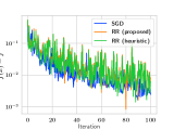
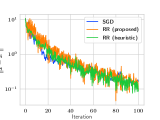
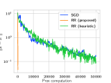
Figure 1: Experimental results for problem (14).

Homogeneous data. For simplicity, in the homogeneous (i.e., i.i.d.) data case we provide guarantees without the proximal operator. Since then we have $F_{1}(x)=\dotsb=F_{M}(x)$, for any $m$ it holds $\nabla F_{m}(x_{\ast})=0$, and thus $\sigma_{m,\ast}^{2}=\frac{1}{n}\sum_{j=1}^{n}\|\nabla f_{mj}(x_{\ast})\|^{2}$. The full variance is then given by

$$\textstyle\sum\limits_{m=1}^{M}\sigma_{m,\ast}^{2}=\frac{1}{n}\sum\limits_{m=1}^{M}\sum\limits_{i=1}^{n}\|\nabla f_{mi}(x_{\ast})\|^{2}=\frac{N}{n}\sigma_{\ast}^{2}=M\sigma_{\ast}^{2},$$

where $\sigma_{\ast}^{2}\overset{\text{def}}{=}\frac{1}{N}\sum_{i=1}^{n}\sum_{m=1}^{M}\|\nabla f_{mi}(x_{\ast})\|^{2}$ is the variance of the gradients over all data.

Theorem 8.

Let $R(x)\equiv 0$ (no prox) and the data be i.i.d., that is $\nabla F_{m}(x_{\ast})=0$ for any $m$, where $x_{\ast}$ is the solution of (7). If each $f_{mj}$ is $L_{\max}$-smooth and $\mu$-strongly convex, then the iterates of Algorithm 3 satisfy

$$\textstyle\mathbb{E}\left[\|x_{T}-x_{\ast}\|^{2}\right]\leq(1-\gamma\mu)^{nT}\|x_{0}-x_{\ast}\|^{2}+\frac{\gamma^{2}L_{\max}N\sigma_{\ast}^{2}}{M\mu},$$

where $\sigma_{\ast}^{2}\overset{\text{def}}{=}\frac{1}{N}\sum_{i=1}^{n}\sum_{m=1}^{M}\|\nabla f_{mi}(x_{\ast})\|^{2}$.

The most important part of this result is that the last term in Theorem 8 has a factor of $M$ in the denominator, meaning that the convergence bound improves with the number of devices involved.

8 Experiments

We look at the logistic regression loss with the elastic net regularization,

$$\textstyle\smash{\frac{1}{N}\sum\limits_{i=1}^{N}f_{i}(x)+\lambda_{1}\|x\|_{1}+\frac{\lambda_{2}}{2}\|x\|^{2}},$$ (14)

where each $f_{i}:\mathbb{R}^{d}\to\mathbb{R}$ is defined as

$$f_{i}(x)\overset{\text{def}}{=}-\big{(}b_{i}\log\big{(}h(a_{i}^{\top}x)\big{)}+(1-b_{i})\log\big{(}1-h(a_{i}^{\top}x)\big{)}\big{)}$$

and where $(a_{i},b_{i})\in\mathbb{R}^{d}\times\{0,1\}$, $i=1,\dotsc,N$ are the data samples, $h\colon t\to 1/(1+e^{-t})$ is the sigmoid function, and $\lambda_{1},\lambda_{2}\geq 0$ are parameters. We set minibatch sizes to 1 for all methods and use theoretical stepsizes, without any tuning. We denote the version of RR that performs proximal operator step after each iteration as ‘RR (heuristic)’. We give more details in the supplementary. From the experiments, we can see that all methods behave more or less the same way. However, the algorithm that we propose needs only a small fraction of proximal operator evaluations, which gives it a huge advantage whenever the operator takes more time to compute than stochastic gradients.

Supplementary Material

9 Basic notions and preliminaries

We say that an extended real-valued function $\phi:\mathbb{R}^{d}\to\mathbb{R}\cup\{+\infty\}$ is proper if its domain, ${\rm dom}\;\phi\overset{\text{def}}{=}\{x:\phi(x)<+\infty\}$, is nonempty. We say that it is convex (resp. closed) if its epigraph, ${\rm epi}\;\phi\overset{\text{def}}{=}\{(x,t)\in\mathbb{R}^{d}\times\mathbb{R}\;:\;\phi(x)\leq t\}$, is a convex (resp. closed) set. Equivalently, $\phi$ is convex if ${\rm dom}\;\phi$ is a convex set and $\phi(\alpha x+(1-\alpha)y)\leq\alpha\phi(x)+(1-\alpha)\phi(y)$ for all $x,y\in{\rm dom}\;\phi$ and $\alpha\in(0,1)$. Finally, $\phi$ is $\mu$-strongly convex if $\phi(x)-\frac{\mu}{2}\left\lVert x\right\rVert^{2}$ is convex, and $L$-smooth if $\frac{L}{2}\left\lVert x\right\rVert^{2}-\phi(x)$ is convex.

These notions have a more useful characterization in the case of real valued and continuously differentiable functions $\phi:\mathbb{R}^{d}\to\mathbb{R}$. The Bregman divergence of such $\phi$ is defined by $D_{\phi}(x,y)\overset{\text{def}}{=}\phi(x)-\phi(y)-\left\langle\nabla\phi(y),x-y\right\rangle.$ A continuously differentiable function $\phi$ is called $\mu$-strongly convex if

$$\tfrac{\mu}{2}\left\lVert x-y\right\rVert^{2}\leq D_{\phi}(x,y),\qquad\forall x,y\in\mathbb{R}^{d}.$$

It is convex if this holds with $\mu=0$. Moreover, a continuously differentiable function $\phi$ is called $L$-smooth if

$$D_{\phi}(x,y)\leq\tfrac{L}{2}\left\lVert x-y\right\rVert^{2},\qquad\forall x,y\in\mathbb{R}^{d}.$$ (15)

Finally, we define $[n]\overset{\text{def}}{=}\{1,2,\dots,n\}$.

9.1 Properties of the proximal operator

Before we proceed to the proofs of convergence, we should state some basic and well-known properties of the regularized objectives. The following lemma explains why the solution of (1) is a fixed point of the proximal-gradient step for any stepsize.

Lemma 4.

Let Assumption 1 be satisfied. Then point $x_{\ast}$ is a minimizer of $P(x)=f(x)+\psi(x)$ if and only if for any $\gamma,b>0$ we have

$$x_{\ast}=\mathrm{prox}_{\gamma n\psi}(x_{\ast}-\gamma b\nabla f(x_{\ast})).$$

Proof.

This follows by writing the first-order optimality conditions for problem (1), see (Parikh & Boyd, 2014, p.32) for a full proof. ∎

The lemma above only shows that proximal-gradient step does not hurt if we are at the solution. In addition, we will rely on the following a bit stronger result which postulates that the proximal operator is a contraction (resp. strong contraction) if the regularizer $\psi$ is convex (resp. strongly convex).

Lemma 5.

Let Assumption 1 be satisfied. If $\psi$ is $\mu$-strongly convex with $\mu\geq 0$, then for any $\gamma>0$ we have

$$\|\mathrm{prox}_{\gamma n\psi}(x)-\mathrm{prox}_{\gamma n\psi}(y)\|^{2}\leq\frac{1}{1+2\gamma\mu n}\|x-y\|^{2},$$ (16)

for all $x,y\in\mathbb{R}^{d}$.

Proof.

Let $u\overset{\text{def}}{=}\mathrm{prox}_{\gamma n\psi}(x)$ and $v\overset{\text{def}}{=}\mathrm{prox}_{\gamma n\psi}(y)$. By definition, $u=\operatorname*{\arg\!\min}_{w}\{\psi(w)+\frac{1}{2\gamma n}\|w-x\|^{2}\}$. By first-order optimality, we have $0\in\partial\psi(u)+\frac{1}{\gamma n}(u-x)$ or simply $x-u\in\gamma n\partial\psi(u)$. Using a similar argument for $v$, we get $x-u-(y-v)\in\gamma n(\partial\psi(u)-\partial\psi(v))$. Thus, by strong convexity of $\psi$, we get

$$\langle x-u-(y-v),u-v\rangle\geq\gamma\mu n\|u-v\|^{2}.$$

Hence,

$$\|x-y\|^{2} =\|u-v+(x-u-(y-v))\|^{2}$$

$$=\|u-v\|^{2}+2\langle x-u-(y-v),u-v\rangle+\|x-u-(y-v)\|^{2}$$

$$\geq\|u-v\|^{2}+2\langle x-u-(y-v),u-v\rangle$$

$$\geq(1+2\gamma\mu n)\|u-v\|^{2}.$$ ∎

10 Proof of Theorem 1

Proof.

By the $L_{i}$-smoothness of $f_{i}$ and the definition of $x_{\ast}^{i}$, we can replace the Bregman divergence in (4) with the bound

$$\mathbb{E}\left[D_{f_{\pi_{i}}}(x_{\ast}^{i},x_{\ast})\right]\;\overset{\eqref{eq:L-smooth-intro}}{\leq}\;\mathbb{E}\left[\frac{L_{\pi_{i}}}{2}\left\lVert x_{\ast}^{i}-x_{\ast}\right\rVert^{2}\right] \leq\frac{L_{\max}}{2}\mathbb{E}\left[\|x_{\ast}^{i}-x_{\ast}\|^{2}\right]$$

$$\overset{\eqref{eq:x_ast_i}}{=}\frac{\gamma^{2}L_{\max}}{2}\mathbb{E}\Biggl{[}\biggl{\|}\sum_{j=0}^{i-1}\nabla f_{\pi_{j}}(x_{\ast})\biggr{\|}^{2}\Biggr{]}$$

$$=\frac{\gamma^{2}L_{\max}i^{2}}{2}\mathbb{E}\Biggl{[}\biggl{\|}\frac{1}{i}\sum_{j=0}^{i-1}\nabla f_{\pi_{j}}(x_{\ast})\biggr{\|}^{2}\Biggr{]}$$

$$=\frac{\gamma^{2}L_{\max}i^{2}}{2}\mathbb{E}\left[\left\lVert\bar{X}_{\pi}\right\rVert^{2}\right],$$ (17)

where $\bar{X}_{\pi}=\frac{1}{j}\sum_{j=0}^{i-1}X_{\pi_{j}}$ with $X_{j}\overset{\text{def}}{=}\nabla f_{j}(x_{\ast})$ for $j=1,2,\dots,n$. Since $\bar{X}=\nabla f(x_{\ast})$, by applying Lemma 1 we get

$$\mathbb{E}\left[\left\lVert\bar{X}_{\pi}\right\rVert^{2}\right]\;=\;\left\lVert\bar{X}\right\rVert^{2}+\mathbb{E}\left[\left\lVert\bar{X}_{\pi}-\bar{X}\right\rVert^{2}\right]\;\overset{\eqref{eq:b97fg07gdf_08yf8d}+\eqref{eq:UG(*G(DG(*DGg87gf7ff}}{=}\;\left\lVert\nabla f(x_{\ast})\right\rVert^{2}+\frac{n-i}{i(n-1)}\sigma_{\ast}^{2}.$$ (18)

It remains to combine (17) and (18), use the bounds $i^{2}\leq n^{2}$ and $i(n-i)\leq\frac{n(n-1)}{2}$, which holds for all $i\in\{1,2,\dots,n-1\}$, and divide both sides of the resulting inequality by $\gamma^{2}$. ∎

11 Main convergence proofs

11.1 A key lemma for shuffling-based methods

The intermediate limit points $x_{\ast}^{i}$ are extremely important for showing tight convergence guarantees for Random Reshuffling even without proximal operator. The following lemma illustrates that by giving a simple recursion, whose derivation follows (Mishchenko et al., 2020, Proof of Theorem 1). The proof is included for completeness.

Lemma 6 (Theorem 1 in (Mishchenko et al., 2020)).

Suppose that each $f_{i}$ is $L_{i}$-smooth and $\lambda$-strongly convex (where $\lambda=0$ means each $f_{i}$ is just convex). Then the inner iterates generated by Algorithm 1 satisfy

$$\mathbb{E}\left[\left\lVert x_{t}^{i+1}-x_{\ast}^{i+1}\right\rVert^{2}\right]\leq\left(1-\gamma\lambda\right)\mathbb{E}\left[\left\lVert x_{t}^{i}-x_{\ast}^{i}\right\rVert^{2}\right]-2\gamma\left(1-\gamma L_{\max}\right)\mathbb{E}\left[D_{f_{\pi_{i}}}(x_{t}^{i},x_{\ast})\right]+2\gamma^{3}\sigma_{\mathrm{rad}}^{2},$$ (19)

where $x_{\ast}^{i}$ is as in (3) and $x_{\ast}$ is any minimizer of $P$.

Proof.

By definition of $x_{t}^{i+1}$ and $x_{\ast}^{i+1}$, we have

$$\begin{split}\mathbb{E}\left[\left\lVert x_{t}^{i+1}-x_{*}^{i+1}\right\rVert^{2}\right]&=\mathbb{E}\left[\left\lVert x_{t}^{i}-x_{*}^{i}\right\rVert^{2}\right]-2\gamma\mathbb{E}\left[\langle\nabla f_{\pi_{i}}(x_{t}^{i})-\nabla f_{\pi_{i}}(x_{*}),x_{t}^{i}-x_{*}^{i}\rangle\right]\\ &\qquad+\gamma^{2}\mathbb{E}\left[\left\lVert\nabla f_{\pi_{i}}(x_{t}^{i})-\nabla f_{\pi_{i}}(x_{*})\right\rVert^{2}\right].\end{split}$$ (20)

Note that the third term in (20) can be bounded as

$${\left\lVert\nabla f_{\pi_{i}}(x_{t}^{i})-\nabla f_{\pi_{i}}(x_{t}^{i})\right\rVert}^{2}\leq 2L_{\max}\cdot D_{f_{\pi_{i}}}(x_{t}^{i},x_{\ast}).$$ (21)

We may rewrite the second term in (20) using the three-point identity (Chen & Teboulle, 1993, Lemma 3.1) as

$$\left\langle\nabla f_{\pi_{i}}(x_{t}^{i})-\nabla f_{\pi_{i}}(x_{\ast}),x_{t}^{i}-x_{\ast}^{i}\right\rangle=D_{f_{\pi_{i}}}(x_{\ast}^{i},x_{t}^{i})+D_{f_{\pi_{i}}}(x_{t}^{i},x_{\ast})-D_{f_{\pi_{i}}}(x_{\ast}^{i},x_{\ast}).$$ (22)

Combining (20), (21), and (22) we obtain

$$\begin{split}\mathbb{E}\left[\left\lVert x_{t}^{i+1}-x_{\ast}^{i+1}\right\rVert^{2}\right]\leq\mathbb{E}\left[\left\lVert x_{t}^{i}-x_{\ast}^{i}\right\rVert^{2}\right]&-2\gamma\cdot\mathbb{E}\left[D_{f_{\pi_{i}}}(x_{\ast}^{i},x_{t}^{i})\right]+2\gamma\cdot\mathbb{E}\left[D_{f_{\pi_{i}}}(x_{\ast}^{i},x_{\ast})\right]\\ &-2\gamma\left(1-\gamma L_{\max}\right)\mathbb{E}\left[D_{f_{\pi_{i}}}(x_{t}^{i},x_{\ast})\right].\end{split}$$ (23)

Using $\lambda$-strong convexity of $f_{\pi_{i}}$, we derive

$$\frac{\lambda}{2}{\left\lVert x_{t}^{i}-x_{\ast}^{i}\right\rVert}^{2}\leq D_{f_{\pi_{i}}}(x_{\ast}^{i},x_{t}^{i}).$$ (24)

Furthermore, by the definition of shuffling radius (Definition 1), we have

$$\mathbb{E}\left[D_{f_{\pi_{i}}}(x_{\ast}^{i},x_{\ast})\right]\leq\max_{i=1,\ldots,n-1}\mathbb{E}\left[D_{f_{\pi_{i}}}(x_{\ast}^{i},x_{\ast})\right]=\gamma^{2}\sigma_{\mathrm{rad}}^{2}.$$ (25)

Using (24) and (25) in (23) yields (19). ∎

11.2 Proof of Theorem 2

Proof.

Starting with Lemma 6 with $\lambda=\mu$, we have

$$\begin{split}\mathbb{E}\left[\left\lVert x_{t}^{i+1}-x_{\ast}^{i+1}\right\rVert^{2}\right]\leq\left(1-\gamma\mu\right)\mathbb{E}\left[\left\lVert x_{t}^{i}-x_{\ast}^{i}\right\rVert^{2}\right]-2\gamma\left(1-\gamma L_{\max}\right)\mathbb{E}\left[D_{f_{\pi_{i}}}(x_{t}^{i},x_{\ast})\right]+2\gamma^{3}\sigma_{\mathrm{rad}}^{2}.\end{split}$$

Since $D_{f_{\pi}}(x_{t}^{i},x_{\ast})$ is a Bregman divergence of a convex function, it is nonnegative. Combining this with the fact that the stepsize satisfies $\gamma\leq\frac{1}{L_{\max}}$, we have

$$\mathbb{E}\left[\left\lVert x_{t}^{i+1}-x_{\ast}^{i+1}\right\rVert^{2}\right]\leq\left(1-\gamma\mu\right)\mathbb{E}\left[\left\lVert x_{t}^{i}-x_{\ast}^{i}\right\rVert^{2}\right]+2\gamma^{3}\sigma_{\mathrm{rad}}^{2}.$$

Unrolling this recursion for $n$ steps, we get

$$\mathbb{E}\left[\left\lVert x_{t}^{n}-x_{\ast}^{n}\right\rVert^{2}\right] \leq\left(1-\gamma\mu\right)^{n}\mathbb{E}\left[\left\lVert x_{t}^{0}-x_{\ast}^{0}\right\rVert^{2}\right]+2\gamma^{3}\sigma_{\mathrm{rad}}^{2}\left(\sum_{j=0}^{n-1}\left(1-\gamma\mu\right)^{j}\right)$$

$$=\left(1-\gamma\mu\right)^{n}\mathbb{E}\left[\left\lVert x_{t}-x_{\ast}\right\rVert^{2}\right]+2\gamma^{3}\sigma_{\mathrm{rad}}^{2}\left(\sum_{j=0}^{n-1}\left(1-\gamma\mu\right)^{j}\right),$$ (26)

where we used the fact that $x_{t}^{0}-x_{\ast}^{0}=x_{t}-x_{\ast}$. Since $x_{\ast}$ minimizes $P$, we have by Lemma 4 that

$$x_{\ast}=\mathrm{prox}_{\gamma n\psi}\left(x_{\ast}-\gamma\sum_{i=0}^{n-1}\nabla f_{\pi_{i}}(x_{\ast})\right)=\mathrm{prox}_{\gamma n\psi}\left(x_{\ast}^{n}\right).$$

Moreover, by Lemma 5 we obtain that

$${\left\lVert x_{t+1}-x_{\ast}\right\rVert}^{2}={\left\lVert\mathrm{prox}_{\gamma n\psi}(x_{t}^{n})-\mathrm{prox}_{\gamma n\psi}(x_{\ast}^{n})\right\rVert}^{2}\leq{\left\lVert x_{t}^{n}-x_{\ast}^{n}\right\rVert}^{2}.$$

Using this in (26) yields

$$\mathbb{E}\left[\left\lVert x_{t+1}-x_{\ast}\right\rVert^{2}\right]\leq\left(1-\gamma\mu\right)^{n}\mathbb{E}\left[\left\lVert x_{t}-x_{\ast}\right\rVert^{2}\right]+2\gamma^{3}\sigma_{\mathrm{rad}}^{2}\left(\sum_{j=0}^{n-1}\left(1-\gamma\mu\right)^{j}\right).$$

We now unroll this recursion again for $T$ steps

$$\begin{split}\mathbb{E}\left[\left\lVert x_{T}-x_{\ast}\right\rVert^{2}\right]\leq\left(1-\gamma\mu\right)^{nT}\mathbb{E}\left[\left\lVert x_{0}-x_{\ast}\right\rVert^{2}\right]+2\gamma^{3}\sigma_{\mathrm{rad}}^{2}\left(\sum_{j=0}^{n-1}\left(1-\gamma\mu\right)^{j}\right)\left(\sum_{i=0}^{T-1}\left(1-\gamma\mu\right)^{ni}\right)\end{split}.$$ (27)

Following Mishchenko et al. (2020), we rewrite and bound the product in the last term as

$$\left(\sum_{j=0}^{n-1}\left(1-\gamma\mu\right)^{j}\right)\left(\sum_{i=0}^{T-1}\left(1-\gamma\mu\right)^{ni}\right) =\sum_{j=0}^{n-1}\sum_{i=0}^{T-1}\left(1-\gamma\mu\right)^{ni+j}$$

$$=\sum_{k=0}^{nT-1}\left(1-\gamma\mu\right)^{k}$$

$$\leq\sum_{k=0}^{\infty}\left(1-\gamma\mu\right)^{k}\quad=\frac{1}{\gamma\mu}.$$

It remains to plug this bound into (27). ∎

11.3 Proof of Theorem 4

Proof.

Starting with Lemma 6 with $\lambda=0$, we have

$$\mathbb{E}\left[\left\lVert x_{t}^{i+1}-x_{\ast}^{i+1}\right\rVert^{2}\right]\leq\mathbb{E}\left[\left\lVert x_{t}^{i}-x_{\ast}^{i}\right\rVert^{2}\right]-2\gamma\left(1-\gamma L_{\max}\right)\mathbb{E}\left[D_{f_{\pi_{i}}}(x_{t}^{i},x_{\ast})\right]+2\gamma^{3}\sigma_{\mathrm{rad}}^{2}.$$

Since $\gamma\leq\frac{1}{L_{\max}}$ and $D_{f_{\pi}}(x_{t}^{i},x_{\ast})$ is nonnegative we may simplify this to

$$\mathbb{E}\left[\left\lVert x_{t}^{i+1}-x_{\ast}^{i+1}\right\rVert^{2}\right]\leq\mathbb{E}\left[\left\lVert x_{t}^{i}-x_{\ast}^{i}\right\rVert^{2}\right]+2\gamma^{3}\sigma_{\mathrm{rad}}^{2}.$$

Unrolling this recursion over an epoch we have

$$\mathbb{E}\left[\left\lVert x_{t}^{n}-x_{\ast}^{n}\right\rVert^{2}\right]\leq\mathbb{E}\left[\left\lVert x_{t}^{0}-x_{\ast}^{0}\right\rVert^{2}\right]+2\gamma^{3}\sigma_{\mathrm{rad}}^{2}n=\mathbb{E}\left[\left\lVert x_{t}-x_{\ast}\right\rVert^{2}\right]+2\gamma^{3}\sigma_{\mathrm{rad}}^{2}n.$$ (28)

Since $x_{\ast}$ minimizes $P$, we have by Lemma 4 that

$$x_{\ast}=\mathrm{prox}_{\gamma n\psi}\left(x_{\ast}-\gamma\sum_{i=0}^{n-1}\nabla f_{\pi_{i}}(x_{\ast})\right)=\mathrm{prox}_{\gamma n\psi}\left(x_{\ast}^{n}\right).$$

Hence, $x_{t+1}-x_{\ast}=\mathrm{prox}_{\gamma n\psi}(x_{t}^{n})-\mathrm{prox}_{\gamma n\psi}(x_{\ast}^{n})$. We may now use Lemma 5 to get

$$\left(1+2\gamma\mu n\right)\mathbb{E}\left[\left\lVert x_{t+1}-x_{\ast}\right\rVert^{2}\right]\leq\mathbb{E}\left[\left\lVert x_{t}^{n}-x_{\ast}^{n}\right\rVert^{2}\right].$$

Combining this with (28), we obtain

$$\mathbb{E}\left[\left\lVert x_{t+1}-x_{\ast}\right\rVert^{2}\right]\leq\frac{1}{1+2\gamma\mu n}\mathbb{E}\left[\left\lVert x_{t}-x_{\ast}\right\rVert^{2}\right]+\frac{2\gamma^{3}\sigma_{\mathrm{rad}}^{2}n}{1+2\gamma\mu n}.$$

We may unroll this recursion again, this time for $T$ steps, and then use that $\sum_{j=1}^{T-1}\left(1+2\gamma\mu n\right)^{-j}\leq\sum_{j=1}^{\infty}\left(1+2\gamma\mu n\right)^{-j}=1/(2\gamma\mu n)$:

$$\mathbb{E}\left[\left\lVert x_{T}-x_{\ast}\right\rVert^{2}\right] \leq\left(1+2\gamma\mu n\right)^{-T}\mathbb{E}\left[\left\lVert x_{0}-x_{\ast}\right\rVert^{2}\right]+\frac{2\gamma^{3}\sigma_{\mathrm{rad}}^{2}n}{1+2\gamma\mu n}\Biggl{(}\sum_{j=0}^{T-1}\left(1+2\gamma\mu n\right)^{-j}\Biggr{)}$$

$$=\left(1+2\gamma\mu n\right)^{-T}\mathbb{E}\left[\left\lVert x_{0}-x_{\ast}\right\rVert^{2}\right]+2\gamma^{3}\sigma_{\mathrm{rad}}^{2}n\Biggl{(}\sum_{j=1}^{T}\left(1+2\gamma\mu n\right)^{-j}\Biggr{)}$$

$$\leq\left(1+2\gamma\mu n\right)^{-T}\mathbb{E}\left[\left\lVert x_{0}-x_{\ast}\right\rVert^{2}\right]+2\gamma^{3}\sigma_{\mathrm{rad}}^{2}n\frac{1}{2\gamma\mu n}$$

$$=\left(1+2\gamma\mu n\right)^{-T}\mathbb{E}\left[\left\lVert x_{0}-x_{\ast}\right\rVert^{2}\right]+\frac{\gamma^{2}\sigma_{\mathrm{rad}}^{2}}{\mu}.$$ ∎

12 Convergence of SGD (Proof of Theorem 3)

Proof.

We will prove the case when $\psi$ is $\mu$-strongly convex. The other result follows as a straightforward special case of (Gorbunov et al., 2020, Theorem 4.1). We start by analyzing one step of SGD with stepsize $\gamma_{k}=\gamma$ and using Lemma 4

$${\left\lVert x_{k+1}-x_{\ast}\right\rVert}^{2} ={\left\lVert\mathrm{prox}_{\gamma\psi}(x_{k}-\gamma\nabla f_{\xi}(x_{k}))-\mathrm{prox}_{\gamma\psi}(x_{\ast}-\gamma\nabla f(x_{\ast}))\right\rVert}^{2}$$

$$\leq\frac{1}{1+2\gamma\mu}{\left\lVert x_{k}-\gamma\nabla f_{\xi}(x_{k})-(x_{\ast}-\gamma\nabla f(x_{\ast}))\right\rVert}^{2}.$$ (29)

We may write the squared norm term in (29) as

$$\begin{split}{\left\lVert x_{k}-\gamma\nabla f_{\xi}(x_{k})-(x_{\ast}-\gamma\nabla f(x_{\ast}))\right\rVert}^{2}&={\left\lVert x_{k}-x_{\ast}\right\rVert}^{2}-2\gamma\left\langle x_{k}-x_{\ast},\nabla f_{\xi}(x_{k})-\nabla f(x_{\ast})\right\rangle\\ &\qquad+\gamma^{2}{\left\lVert\nabla f_{\xi}(x_{k})-\nabla f(x_{\ast})\right\rVert}^{2}.\end{split}$$ (30)

We denote by $\mathbb{E}_{k}\left[\cdot\right]$ expectation conditional on $x_{k}$. Note that the gradient estimate is conditionally unbiased, i.e., that $\mathbb{E}_{k}\left[\nabla f_{\xi}(x_{k})\right]=\frac{1}{n}\sum_{i=1}^{n}\nabla f_{i}(x_{k})=\nabla f(x_{k})$. Hence, taking conditional expectation in (30) and using unbiasedness we have

$$\begin{split}\mathbb{E}_{k}\left[\left\lVert x_{k}-\gamma\nabla f_{\xi}(x_{k})-(x_{\ast}-\gamma\nabla f(x_{\ast}))\right\rVert^{2}\right]&={\left\lVert x_{k}-x_{\ast}\right\rVert}^{2}-2\gamma\left\langle x_{k}-x_{\ast},\nabla f(x_{k})-\nabla f(x_{\ast})\right\rangle\\ &\qquad+\gamma^{2}\mathbb{E}_{k}\left[\left\lVert\nabla f_{\xi}(x_{k})-\nabla f(x_{\ast})\right\rVert^{2}\right].\end{split}$$ (31)

By the convexity of $f$ we have

$$\left\langle x_{k}-x_{\ast},\nabla f(x_{k})-\nabla f(x_{\ast})\right\rangle\geq D_{f}(x_{k},x_{\ast}).$$

Furthermore, we may estimate the third term in (31) by first using the fact that ${\left\lVert x+y\right\rVert}^{2}\leq 2{\left\lVert x\right\rVert}^{2}+2{\left\lVert y\right\rVert}^{2}$ for any two vectors $x,y\in\mathbb{R}^{d}$

$$\mathbb{E}_{k}\left[{\left\lVert\nabla f_{\xi}(x_{k})-\nabla f(x_{\ast})\right\rVert}^{2}\right] \leq 2\mathbb{E}_{k}\left[\left\lVert\nabla f_{\xi}(x_{k})-\nabla f_{\xi}(x_{\ast})\right\rVert^{2}\right]+2\mathbb{E}_{k}\left[\left\lVert\nabla f_{\xi}(x_{\ast})-\nabla f(x_{\ast})\right\rVert^{2}\right]$$

$$=2\mathbb{E}_{k}\left[\left\lVert\nabla f_{\xi}(x_{k})-\nabla f_{\xi}(x_{\ast})\right\rVert^{2}\right]+2\sigma_{\ast}^{2}.$$

We now use that by the $L_{\max}$-smoothness of $f_{i}$ we have that

$${\left\lVert\nabla f_{i}(x_{k})-\nabla f_{i}(x_{\ast})\right\rVert}^{2}\leq 2L_{\max}\cdot D_{f_{i}}(x_{k},x_{\ast}).$$

Hence

$$\mathbb{E}_{k}\left[\left\lVert\nabla f_{\xi}(x_{k})-\nabla f_{\xi}(x_{\ast})\right\rVert^{2}\right] =\frac{1}{n}\sum_{i=1}^{n}{\left\lVert\nabla f_{i}(x_{k})-\nabla f_{i}(x_{\ast})\right\rVert}^{2}$$

$$\leq\frac{2L_{\max}}{n}\sum_{i=1}^{n}\left[f_{i}(x_{k})-f_{i}(x_{\ast})-\left\langle\nabla f_{i}(x_{\ast}),x_{k}-x_{\ast}\right\rangle\right]$$

$$=2L_{\max}\left[f(x_{k})-f(x_{\ast})-\left\langle\nabla f(x_{\ast}),x_{k}-x_{\ast}\right\rangle\right]$$

$$=2L_{\max}D_{f}(x_{k},x_{\ast}).$$ (32)

Combining equations (31)–(32) we obtain

$$\begin{split}\mathbb{E}_{k}\left[\left\lVert x_{k}-\gamma\nabla f_{\xi}(x_{k})-(x_{\ast}-\gamma\nabla f(x_{\ast}))\right\rVert^{2}\right]&\leq{\left\lVert x_{k}-x_{\ast}\right\rVert}^{2}-2\gamma\left(1-2\gamma L_{\max}\right)D_{f}(x_{k},x_{\ast})\\ &\qquad+2\gamma^{2}\sigma_{\ast}^{2}.\end{split}$$

Since $\gamma\leq\frac{1}{2L_{\max}}$ by assumption we have that $1-2\gamma L_{\max}\geq 0$. Since $D_{f}(x_{k},x_{\ast})\geq 0$ by the convexity of $f$ we arrive at

$$\mathbb{E}_{k}\left[\left\lVert x_{k}-\gamma\nabla f_{\xi}(x_{k})-(x_{\ast}-\gamma\nabla f(x_{\ast}))\right\rVert^{2}\right]\leq{\left\lVert x_{k}-x_{\ast}\right\rVert}^{2}+2\gamma^{2}\sigma_{\ast}^{2}.$$

Taking unconditional expectation and combining (34) with the last equation we have

$$\mathbb{E}\left[\left\lVert x_{k+1}-x_{\ast}\right\rVert^{2}\right] \leq\frac{1}{1+2\gamma\mu}\left(\mathbb{E}\left[\left\lVert x_{k}-x_{\ast}\right\rVert^{2}\right]+2\gamma^{2}\sigma_{\ast}^{2}\right)$$

$$=\frac{1}{1+2\gamma\mu}\mathbb{E}\left[\left\lVert x_{k}-x_{\ast}\right\rVert^{2}\right]+\frac{2\gamma^{2}\sigma_{\ast}^{2}}{1+2\gamma\mu}$$

$$\leq\frac{1}{1+2\gamma\mu}\mathbb{E}\left[\left\lVert x_{k}-x_{\ast}\right\rVert^{2}\right]+2\gamma^{2}\sigma_{\ast}^{2}.$$

To simplify this further, we use that for any $x\leq\frac{1}{2}$ we have that $\frac{1}{1+2x}\leq 1-x$ and that $\gamma\mu\leq\frac{\mu}{2L_{\max}}\leq\frac{1}{2}$, hence

$$\mathbb{E}\left[\left\lVert x_{k+1}-x_{\ast}\right\rVert^{2}\right]\leq\left(1-\gamma\mu\right)\mathbb{E}\left[\left\lVert x_{k}-x_{\ast}\right\rVert^{2}\right]+2\gamma^{2}\sigma_{\ast}^{2}.$$

Recursing the above inequality for $K$ steps yields

$$\mathbb{E}\left[\left\lVert x_{K}-x_{\ast}\right\rVert^{2}\right] \leq\left(1-\gamma\mu\right)^{K}{\left\lVert x_{0}-x_{\ast}\right\rVert}^{2}+2\gamma^{2}\sigma_{\ast}^{2}\left(\sum_{k=0}^{K-1}\left(1-\gamma\mu\right)^{k}\right)$$

$$\leq\left(1-\gamma\mu\right)^{K}{\left\lVert x_{0}-x_{\ast}\right\rVert}^{2}+2\gamma^{2}\sigma_{\ast}^{2}\left(\sum_{k=0}^{\infty}\left(1-\gamma\mu\right)^{k}\right)$$

$$=\left(1-\gamma\mu\right)^{K}{\left\lVert x_{0}-x_{\ast}\right\rVert}^{2}+\frac{2\gamma\sigma_{\ast}^{2}}{\mu}.$$ ∎

13 Proofs for decreasing stepsize

We first state and prove the following algorithm-independent lemma. This lemma plays a key role in the proof of Theorem 5 and is heavily inspired by the stepsize schemes of Stich (2019) and Khaled & Richtárik (2020) and their proofs.

Lemma 7.

Suppose that there exist constants $a,b,c\geq 0$ such that for all $\gamma_{t}\leq\frac{1}{b}$ we have

$$\left(1+\gamma_{t}an\right)r_{t+1}\leq r_{t}+\gamma_{t}^{3}c.$$ (33)

Fix $T>0$. Let $t_{0}=\lceil\frac{T}{2}\rceil$. Then choosing stepsizes $\gamma_{t}>0$ by

$$\gamma_{t}=\begin{cases}\frac{1}{b},&\text{ if }t\leq t_{0}\text{ or }T\leq\frac{b}{an},\\ \frac{7}{an\left(s+t-t_{0}\right)}&\text{ if }t>t_{0}\text{ and }T>\frac{b}{an},\end{cases}$$

where $s=\frac{7b}{2an}$. Then

$$r_{T}\leq\exp\left(-\frac{nT}{2\left(b/a+n\right)}\right)r_{0}+\frac{1421c}{a^{3}n^{3}T^{2}}.$$

Proof.

If $T\leq\frac{7b}{an}$, then we have $\gamma_{t}=\gamma=\frac{1}{b}$ for all $t$. Hence recursing we have,

$$r_{T} \leq\left(1+\gamma an\right)^{-T}r_{0}+\frac{\gamma^{3}c}{\gamma an}=\left(1+\gamma an\right)^{-T}r_{0}+\frac{\gamma^{2}c}{an}.$$

Note that $\frac{1}{1+x}\leq\exp(-\frac{x}{1+x})$ for all $x$, hence

$$r_{T} \leq\exp\left(-\frac{\gamma anT}{1+\gamma an}\right)r_{0}+\frac{\gamma^{2}c}{an}$$

Substituting for $\gamma$ yields

$$r_{T} \leq\exp\left(-\frac{nT}{b/a+n}\right)r_{0}+\frac{c}{b^{2}an}.$$

Note that by assumption we have $\frac{1}{b}\leq\frac{7}{Tan}$, hence

$$r_{T} \leq\exp\left(-\frac{nT}{b/a+n}\right)r_{0}+\frac{49c}{T^{2}a^{3}n^{3}}.$$ (34)

If $T>\frac{7b}{an}$, then we have for the first phase when $t\leq t_{0}$ with stepsize $\gamma_{t}=\frac{1}{b}$ that

$$r_{t_{0}} \leq\exp\left(-\frac{nt_{0}}{b/a+n}\right)r_{0}+\frac{c}{b^{2}an}\leq\exp\left(-\frac{nT}{2(b/a+n)}\right)r_{0}+\frac{c}{b^{2}an}.$$ (35)

Then for $t>t_{0}$ we have

$$\left(1+\gamma_{t}an\right)r_{t+1}\leq r_{t}+\gamma_{t}^{3}c=r_{t}+\frac{7^{3}c}{a^{3}n^{3}\left(s+t-t_{0}\right)^{3}}.$$

Multiplying both sides by $(s+t-t_{0})^{3}$ yields

$$\left(s+t-t_{0}\right)^{3}\left(1+\gamma_{t}an\right)r_{t+1}\leq\left(s+t-t_{0}\right)^{3}r_{t}+\frac{7^{3}c}{a^{3}n^{3}}.$$ (36)

Note that because $t$ and $t_{0}$ are integers and $t>t_{0}$, we have that $t-t_{0}\geq 1$ and therefore $s+t-t_{0}\geq 1$. We may use this to lower bound the multiplicative factor in the left hand side of (36) as

$$\left(s+t-t_{0}\right)^{3}\left(1+\gamma_{t}an\right) =\left(s+t-t_{0}\right)^{3}\left(1+\frac{7}{s+t-t_{0}}\right)$$

$$=\left(s+t-t_{0}\right)^{3}+7\left(s+t-t_{0}\right)^{2}$$

$$=\left(s+t-t_{0}\right)^{3}+3\left(s+t-t_{0}\right)^{2}+3\left(s+t-t_{0}\right)^{2}+\left(s+t-t_{0}\right)^{2}$$

$$\geq\left(s+t-t_{0}\right)^{3}+3\left(s+t-t_{0}\right)^{2}+3\left(s+t-t_{0}\right)+1$$

$$=\left(s+t+1-t_{0}\right)^{3}.$$ (37)

Using (37) in (36) we obtain

$$\left(s+t+1-t_{0}\right)^{3}r_{t+1}\leq\left(s+t-t_{0}\right)^{3}r_{t}+\frac{7^{3}c}{a^{3}n^{3}}.$$

Let $w_{t}=\left(s+t-t_{0}\right)^{3}$. Then we can rewrite the last inequality as

$$w_{t+1}r_{t+1}-w_{t}r_{t}\leq\frac{7^{3}c}{a^{3}n^{3}}.$$

Summing up and telescoping from $t=t_{0}$ to $T$ yields

$$w_{T}r_{T}\leq w_{t_{0}}r_{t_{0}}+\frac{7^{3}c}{a^{3}n^{3}}\left(T-t_{0}\right).$$

Note that $w_{t_{0}}=s^{3}$ and $w_{T}=\left(s+T-t_{0}\right)^{3}$. Hence,

$$r_{T} \leq\frac{s^{3}}{\left(s+T-t_{0}\right)^{3}}r_{t_{0}}+\frac{7^{3}c}{a^{3}n^{3}\left(s+T-t_{0}\right)^{2}}\frac{T-t_{0}}{s+T-t_{0}}$$

$$\leq\frac{s^{3}}{\left(s+T-t_{0}\right)^{3}}r_{t_{0}}+\frac{7^{3}c}{a^{3}n^{3}\left(s+T-t_{0}\right)^{2}}.$$

Since we have $s+T-t_{0}\geq T-t_{0}\geq T/2$, it holds

$$r_{T}\leq\frac{8s^{3}}{T^{3}}r_{t_{0}}+\frac{4\cdot 7^{3}c}{a^{3}n^{3}T^{2}}.$$ (38)

The bound in (35) can be rewritten as

$$\frac{s^{3}}{T^{3}}r_{t_{0}}\leq\frac{s^{3}}{T^{3}}\exp\left(-\frac{nT}{2\left(b/a+n\right)}\right)r_{0}+\frac{s^{3}c}{b^{2}anT^{3}}.$$

We now rewrite the last inequality, use that $T>2s$ and further use the fact that $s=\frac{7b}{2an}$:

$$\frac{s^{3}}{T^{3}}r_{t_{0}} \leq\underbrace{\left(\frac{s}{T}\right)^{3}}_{\leq 1/8}\exp\left(-\frac{nT}{2\left(b/a+n\right)}\right)r_{0}+\frac{s^{2}c}{b^{2}anT^{2}}\underbrace{\left(\frac{s}{T}\right)}_{\leq 1/2}$$

$$\leq\frac{1}{8}\exp\left(-\frac{nT}{2\left(b/a+n\right)}\right)r_{0}+\frac{s^{2}c}{2b^{2}anT^{2}}$$

$$=\frac{1}{8}\exp\left(-\frac{nT}{2\left(b/a+n\right)}\right)r_{0}+\frac{7^{2}c}{8a^{3}n^{3}T^{2}}.$$ (39)

Plugging in the estimate of (39) into (38) we obtain

$$r_{T} \leq\exp\left(-\frac{nT}{2\left(b/a+n\right)}\right)r_{0}+\frac{7^{2}c}{a^{3}n^{3}T^{2}}+\frac{4\cdot 7^{3}c}{a^{3}n^{3}T^{2}}$$

$$=\exp\left(-\frac{nT}{2\left(b/a+n\right)}\right)r_{0}+\frac{1421c}{a^{3}n^{3}T^{2}}.$$ (40)

Taking the maximum of (34) and (40) we see that for any $T>0$ we have

$$r_{T}\leq\exp\left(-\frac{nT}{2\left(b/a+n\right)}\right)r_{0}+\frac{1421c}{a^{3}n^{3}T^{2}}.$$

13.1 Proof of Theorem 5

Proof.

Start with Lemma 6 with $\lambda=0$, $L=L_{\max}$, and $\gamma=\gamma_{t}$,

$$\mathbb{E}\left[\left\lVert x_{t}^{i+1}-x_{\ast}^{i+1}\right\rVert^{2}\right]\leq\mathbb{E}\left[\left\lVert x_{t}^{i}-x_{\ast}^{i}\right\rVert^{2}\right]-2\gamma\left(1-\gamma L_{\max}\right)\mathbb{E}\left[D_{f_{\pi_{i}}}(x_{t}^{i},x_{\ast})\right]+2\gamma_{t}^{3}\sigma_{\mathrm{rad}}^{2}.$$

Since $\gamma\leq\frac{1}{L_{\max}}$ and $D_{f_{\pi}}(x_{t}^{i},x_{\ast})$ is nonnegative we may simplify this to

$$\mathbb{E}\left[\left\lVert x_{t}^{i+1}-x_{\ast}^{i+1}\right\rVert^{2}\right]\leq\mathbb{E}\left[\left\lVert x_{t}^{i}-x_{\ast}^{i}\right\rVert^{2}\right]+2\gamma_{t}^{3}\sigma_{\mathrm{rad}}^{2}.$$

Unrolling this recursion for $n$ steps we get

$$\mathbb{E}\left[\left\lVert x_{t}^{n}-x_{\ast}^{n}\right\rVert^{2}\right]\leq\mathbb{E}\left[\left\lVert x_{t}^{0}-x_{\ast}^{0}\right\rVert^{2}\right]+2n\gamma_{t}^{3}\sigma_{\mathrm{rad}}^{2}.$$

By Lemma 5 and a similar reasoning to Theorem 4 we have

$$\left(1+2\gamma_{t}\mu n\right)\mathbb{E}\left[\left\lVert x_{t+1}-x_{\ast}\right\rVert^{2}\right]\leq\mathbb{E}\left[\left\lVert x_{t}-x_{\ast}\right\rVert^{2}\right]+2\gamma_{t}^{3}\sigma_{\mathrm{rad}}^{2}.$$

We may then use Lemma 7 to obtain that

$$\mathbb{E}\left[\left\lVert x_{T}-x_{\ast}\right\rVert^{2}\right] \leq\exp\left(-\frac{nT}{2(L_{\max}/\mu+n)}\right){\left\lVert x_{0}-x_{\ast}\right\rVert}^{2}+\frac{356\sigma_{\mathrm{rad}}^{2}}{\mu^{3}n^{2}T^{2}}$$

$$=\mathcal{O}\left(\exp\left(-\frac{nT}{\kappa+2n}\right){\left\lVert x_{0}-x_{\ast}\right\rVert}^{2}+\frac{\sigma_{\mathrm{rad}}^{2}}{\mu^{3}n^{2}T^{2}}\right).$$ ∎

14 Proof of Theorem 6 for importance resampling

Proof.

We show that $N\leq 2n$ as the rest of the theorem’s claim trivially follows from Theorem 4. Firstly, note that for any number $a\in\mathbb{R}$ we have $\lceil a\rceil\leq a+1$. Therefore,

$$N=\sum_{i=1}^{n}\left\lceil\frac{L_{i}}{\bar{L}}\right\rceil\leq\sum_{i=1}^{n}\left(\frac{L_{i}}{\bar{L}}+1\right)=n+\sum_{i=1}^{n}\frac{L_{i}}{\bar{L}}=2n.$$

15 Proofs for federated learning

15.1 Lemma for the extended proximal operator

Lemma 8.

Let $\psi_{C}$ be the consensus constraint and $R$ be a closed convex proximable function. Suppose that $x_{1},x_{2},\ldots,x_{M}$ are all in $\mathbb{R}^{d}$. Then,

$$\mathrm{prox}_{\gamma(R+\psi_{C})}(x_{1},\ldots,x_{M})=\mathrm{prox}_{\frac{\gamma}{M}R}(\overline{x}),$$

where $\overline{x}=\frac{1}{M}\sum_{m=1}^{M}x_{m}$.

Proof.

We have,

$$\mathrm{prox}_{\gamma(R+\psi_{C})}(x_{1},\dotsc,x_{M})=\begin{pmatrix}\mathrm{prox}_{\frac{\gamma}{M}R}(\overline{x})\\ \vdots\\ \mathrm{prox}_{\frac{\gamma}{M}R}(\overline{x})\end{pmatrix}\quad\text{with}\quad\overline{x}=\frac{1}{M}\sum_{m=1}^{M}x_{m}.$$

This is a simple consequence of the definition of the proximal operator. Indeed, the result of $\mathrm{prox}_{\gamma(R+\psi_{C})}$ must have blocks equal to some vector $z$ such that

$$z =\operatorname*{\arg\!\min}_{x}\left\{\gamma R(x)+\frac{1}{2}\sum_{m=1}^{M}\|x-x_{m}\|^{2}\right\}$$

$$=\operatorname*{\arg\!\min}_{x}\left\{\gamma R(x)+\frac{1}{2}\sum_{m=1}^{M}\bigl{(}\|x-\overline{x}\|^{2}+2\langle x-\overline{x},\overline{x}-x_{m}\rangle)+\|\overline{x}-x_{m}\|^{2}\bigr{)}\right\}$$

$$=\operatorname*{\arg\!\min}_{x}\left\{\gamma R(x)+\frac{1}{2}M\|x-\overline{x}\|^{2}\right\}\quad=\mathrm{prox}_{\frac{\gamma}{M}R}(\overline{x}).$$

∎

15.2 Proof of Lemma 2

Proof.

Given some vectors ${\boldsymbol{x}},{\boldsymbol{y}}\in\mathbb{R}^{d\cdot M}$, let us use their block representation ${\boldsymbol{x}}=(x_{1}^{\top},\dotsc,x_{M}^{\top})^{\top}$, ${\boldsymbol{y}}=(y_{1}^{\top},\dotsc,y_{M}^{\top})^{\top}$. Since we use the Euclidean norm, we have

$$\|\nabla f_{i}({\boldsymbol{x}})-\nabla f_{i}({\boldsymbol{y}})\|^{2}=\sum_{m=1}^{M}\|\nabla f_{mi}(x_{m})-\nabla f_{mi}(y_{m})\|^{2}\leq\sum_{m=1}^{M}L_{i}^{2}\|x_{m}-y_{m}\|^{2}=L_{i}^{2}\|{\boldsymbol{x}}-{\boldsymbol{y}}\|^{2}.$$

We can obtain a lower bound by doing the same derivation and applying strong convexity instead of smoothness:

$$\sum_{m=1}^{M}\|\nabla f_{mi}(x_{m})-\nabla f_{mi}(y_{m})\|^{2}\geq\mu^{2}\sum_{m=1}^{M}\|x_{m}-y_{m}\|^{2}=\mu^{2}\|{\boldsymbol{x}}-{\boldsymbol{y}}\|^{2}.$$

Thus, we have $\mu\|{\boldsymbol{x}}-{\boldsymbol{y}}\|\leq\|\nabla f_{i}({\boldsymbol{x}})-\nabla f_{i}({\boldsymbol{y}})\|\leq L_{i}\|{\boldsymbol{x}}-{\boldsymbol{y}}\|$, which is exactly $\mu$-strong convexity and $L_{i}$-smoothness of $f_{i}$. ∎

15.3 Proof of Lemma 3

Proof.

By Theorem 1 we have

$$\sigma_{\mathrm{rad}}^{2}\leq\frac{L_{\max}}{2}\Bigl{(}n^{2}\|\nabla f({\boldsymbol{x}}_{\ast})\|^{2}+\frac{n}{2}\sigma_{\ast}^{2}\Bigr{)}.$$

Due to the separable structure of $f$, we have for the variance term

$$n\sigma_{\ast}^{2}\overset{\text{def}}{=}\sum_{i=1}^{n}{\left\lVert\nabla f_{i}({\boldsymbol{x}}_{\ast})-\nabla f({\boldsymbol{x}}_{\ast})\right\rVert}^{2}=\sum_{i=1}^{n}\sum_{m=1}^{M}{\left\lVert\nabla f_{mi}(x_{\ast})-\frac{1}{n}\nabla F_{m}(x_{\ast})\right\rVert}^{2}.$$

The expression inside the summation is not exactly the variance due to the different normalization: $\frac{1}{n}$ instead of $\frac{1}{N_{m}}$. Nevertheless, we can expand the norm and try to get the actual variance:

$$\sum_{i=1}^{n}{\left\lVert\nabla f_{mi}(x_{\ast})-\frac{1}{n}\nabla F_{m}(x_{\ast})\right\rVert}^{2} =\sum_{i=1}^{N_{m}}\biggl{(}{\left\lVert\nabla f_{mi}(x_{\ast})-\frac{1}{N_{m}}\nabla F_{m}(x_{\ast})\right\rVert}^{2}+\Bigl{(}\frac{1}{N_{m}}-\frac{1}{n}\Bigr{)}^{2}{\left\lVert\nabla F_{m}(x_{\ast})\right\rVert}^{2}\biggr{)}$$

$$\quad+2\sum_{i=1}^{N_{m}}\bigl{\langle}\nabla f_{mi}(x_{\ast})-\frac{1}{N_{m}}\nabla F_{m}(x_{\ast}),\Bigl{(}\frac{1}{N_{m}}-\frac{1}{n}\Bigr{)}\nabla F_{m}(x_{\ast})\bigr{\rangle}$$

$$=N_{m}\sigma_{m,\ast}^{2}+N_{m}\Bigl{(}\frac{1}{N_{m}}-\frac{1}{n}\Bigr{)}^{2}{\left\lVert\nabla F_{m}(x_{\ast})\right\rVert}^{2}$$

$$\leq n\sigma_{m,\ast}^{2}+{\left\lVert\nabla F_{m}(x_{\ast})\right\rVert}^{2}.$$

Moreover, the gradient term has the same block structure, so

$$n^{2}\|\nabla f({\boldsymbol{x}}_{\ast})\|^{2}=n^{2}\biggl{\|}\frac{1}{n}\sum_{i=1}^{n}\nabla f_{i}({\boldsymbol{x}}_{\ast})\biggr{\|}^{2}=\sum_{m=1}^{M}{\left\lVert\sum_{i=1}^{n}\nabla f_{mi}(x_{\ast})\right\rVert}^{2}=\sum_{m=1}^{M}\|\nabla F_{m}(x_{\ast})\|^{2}.$$

Plugging the last two bounds back inside the upper bound on $\sigma_{\mathrm{rad}}^{2}$, we deduce the lemma’s statement. ∎

15.4 Proof of Theorem 7

Proof.

Since we assume that $N_{1}=\dotsb=N_{M}=n$, we have $\frac{N}{M}=n$ and the strong convexity constant of$\psi=\frac{N}{n}(R+\psi_{C})$ is equal to $\frac{N}{n}\cdot\frac{\mu}{M}=\mu$. By applying Theorem 4 we obtain

$$\mathbb{E}\left[\left\lVert{\boldsymbol{x}}_{T}-{\boldsymbol{x}}_{\ast}\right\rVert^{2}\right]\leq\left(1+2\gamma\mu n\right)^{-T}{\left\lVert{\boldsymbol{x}}_{0}-{\boldsymbol{x}}_{\ast}\right\rVert}^{2}+\frac{\gamma^{2}\sigma_{\mathrm{rad}}^{2}}{\mu}.$$

Since ${\boldsymbol{x}}_{T}=\mathrm{prox}_{\gamma N(R+\psi_{C})}({\boldsymbol{x}}_{T-1}^{n})$, we have ${\boldsymbol{x}}_{T}\in C$, i.e., all of its blocks are equal to each other and we have ${\boldsymbol{x}}_{T}=(x_{T}^{\top},\dotsc,x_{T}^{\top})^{\top}$. Since we use the Euclidean norm, it also implies

$$\mathbb{E}\left[\left\lVert{\boldsymbol{x}}_{T}-{\boldsymbol{x}}_{\ast}\right\rVert^{2}\right]=M\|x_{T}-x_{\ast}\|^{2}.$$

The same is true for ${\boldsymbol{x}}_{0}$, so we need to divide both sides of the upper bound on $\|{\boldsymbol{x}}_{T}-{\boldsymbol{x}}_{\ast}\|^{2}$ by $M$. Doing so together with applying Lemma 3 yields

$$\mathbb{E}\left[\left\lVert x_{T}-x_{\ast}\right\rVert^{2}\right] \leq\left(1+2\gamma\mu n\right)^{-T}{\left\lVert x_{0}-x_{\ast}\right\rVert}^{2}+\frac{\gamma^{2}\sigma_{\mathrm{rad}}^{2}}{M\mu}$$

$$\leq\left(1+2\gamma\mu n\right)^{-T}{\left\lVert x_{0}-x_{\ast}\right\rVert}^{2}+\frac{\gamma^{2}L_{\max}}{M\mu}\sum_{m=1}^{M}\Bigl{(}\|\nabla F_{m}(x_{\ast})\|^{2}+\frac{n}{4}\sigma_{m,\ast}^{2}\Bigr{)}$$

$$=\left(1+2\gamma\mu n\right)^{-T}{\left\lVert x_{0}-x_{\ast}\right\rVert}^{2}+\frac{\gamma^{2}L_{\max}}{M\mu}\sum_{m=1}^{M}\Bigl{(}\|\nabla F_{m}(x_{\ast})\|^{2}+\frac{N}{4M}\sigma_{m,\ast}^{2}\Bigr{)}.$$

∎

15.5 Proof of Theorem 8

Proof.

According to Lemma 2, each $f_{i}$ is $\mu$-strongly convex and $L_{\max}$-smooth, so we obtain the result by trivially applying Theorem 2 and upper bounding $\sigma_{\mathrm{rad}}^{2}$ the same way as in the proof of Theorem 7. ∎

16 Federated experiments and experimental details

We also compare the performance of FedRR and Local SGD on homogeneous (i.e., i.i.d.) data. Since Local SGD requires smaller stepsizes to converge, it is significantly slower at initialization, as can be seen in Figure 2. FedRR, however, does not need small initial stepsize and very quickly converges to a noisy neighborhood of the solution. The advantage is clear both from the perspective of the number of communication rounds and data passes.

To illustrate the severe impact of the number of local steps in Local SGD we show results with different number of local steps. The blue line shows Local SGD that takes the number of steps equivalent to full pass over the data by each node. The orange line takes 5 times fewer local steps. Clearly, the latter performs better in terms of communication rounds and local steps, making it clear that Local SGD scales worse with the number of local steps. This phenomenon is well-understood and has been in discussed by Khaled et al. (2020).

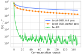
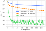
Figure 2: Experimental results for parallel training. Left: comparison in terms of communication rounds, right: in terms of data passes

Implementation details. For each $i$, we have $L_{i}=\frac{1}{4}\|a_{i}\|$. We set $\lambda_{2}=\frac{L}{N}$ and tune $\lambda_{1}$ to obtain a solution with less than 50% coordinates (exact values are provided in the code). We use stepsizes decreasing as $\mathcal{O}(\frac{1}{t})$ for all methods. We use the ‘a1a’ dataset for the experiment with $\ell_{1}$ regularization.

The experiment for the comparison of FedRR and Local SGD uses no $\ell_{1}$ regularization and $\lambda_{2}=\frac{L}{N}$. We choose the stepsizes according to the theory of Local SGD and Fed-RR. As per Theorem 3 in Khaled et al. (2020), the stepsizes for Local SGD must satisfy $\gamma_{t}=\mathcal{O}(1/(LH))$, where $H$ is the number of local steps. The parallelization of local runs is done using the Ray package. We use the ‘mushrooms’ dataset for this experiment.

Proximal operator calculation. As shown by Parikh & Boyd (2014), the proximal operator for $\psi(x)=\lambda_{1}\|x\|_{1}+\frac{\lambda_{2}}{2}\|x\|^{2}$ is given by

$$\mathrm{prox}_{\gamma\psi}(x)=\frac{1}{1+\gamma\lambda_{2}}\mathrm{prox}_{\gamma\lambda_{1}\|\cdot\|_{1}}(x),$$

where the $j$-th coordinate of $\mathrm{prox}_{\gamma\lambda_{1}\|\cdot\|_{1}}(x)$ is

$$[\mathrm{prox}_{\gamma\lambda_{1}\|\cdot\|_{1}}(x)]_{j}=\begin{cases}\mathrm{sign}([x]_{j})(|[x]_{j}|-\gamma\lambda_{1}),&\text{if }|[x]_{j}|\geq\gamma\lambda_{1},\\ 0,&\text{otherwise}.\end{cases}$$

References

• Ahn et al. (2020) Ahn, K., Yun, C., and Sra, S. SGD with shuffling: optimal rates without component convexity and large epoch requirements. arXiv preprint arXiv:2006.06946. Neural Information Processing Systems (NeurIPS) 2020, 2020.
• Beck (2017) Beck, A. First-Order Methods in Optimization. Society for Industrial and Applied Mathematics, Philadelphia, PA, 2017. doi: 10.1137/1.9781611974997.
• Bianchi et al. (2015) Bianchi, P., Hachem, W., and Iutzeler, F. A coordinate descent primal-dual algorithm and application to distributed asynchronous optimization. IEEE Transactions on Automatic Control, 61(10):2947–2957, 2015.
• Bordes et al. (2009) Bordes, A., Bottou, L., and Gallinari, P. SGD-QN: Careful quasi-Newton stochastic gradient descent. 2009.
• Bottou (2009) Bottou, L. Curiously fast convergence of some stochastic gradient descent algorithms. Unpublished open problem offered to the attendance of the SLDS 2009 conference, 2009. URL http://leon.bottou.org/papers/bottou-slds-open-problem-2009.
• Bottou (2012) Bottou, L. Stochastic gradient descent tricks. In Neural networks: Tricks of the trade, pp.  421–436. Springer, 2012.
• Bredies et al. (2010) Bredies, K., Kunisch, K., and Pock, T. Total generalized variation. SIAM Journal on Imaging Sciences, 3(3):492–526, 2010.
• Chen & Teboulle (1993) Chen, G. and Teboulle, M. Convergence Analysis of a Proximal-Like Minimization Algorithm Using Bregman Functions. SIAM Journal on Optimization, 3(3):538–543, 1993. doi: 10.1137/0803026.
• Duchi & Singer (2009) Duchi, J. and Singer, Y. Efficient online and batch learning using forward backward splitting. Journal of Machine Learning Research, 10(Dec):2899–2934, 2009.
• Gorbunov et al. (2020) Gorbunov, E., Hanzely, F., and Richtárik, P. A Unified Theory of SGD: Variance Reduction, Sampling, Quantization and Coordinate Descent. volume 108 of Proceedings of Machine Learning Research, pp. 680–690, Online, 26–28 Aug 2020. PMLR.
• Gower et al. (2019) Gower, R. M., Loizou, N., Qian, X., Sailanbayev, A., Shulgin, E., and Richtárik, P. SGD: General Analysis and Improved Rates. In Chaudhuri, K. and Salakhutdinov, R. (eds.), Proceedings of the 36th International Conference on Machine Learning, volume 97 of Proceedings of Machine Learning Research, pp.  5200–5209, Long Beach, California, USA, 09–15 Jun 2019. PMLR.
• Gower et al. (2020) Gower, R. M., Richtárik, P., and Bach, F. Stochastic quasi-gradient methods: variance reduction via Jacobian sketching. Mathematical Programming, pp.  1–58, 2020. ISSN 0025-5610. doi: 10.1007/s10107-020-01506-0.
• Gürbüzbalaban et al. (2019) Gürbüzbalaban, M., Ozdaglar, A., and Parrilo, P. A. Why random reshuffling beats stochastic gradient descent. Mathematical Programming, Oct 2019. ISSN 1436-4646. doi: 10.1007/s10107-019-01440-w.
• Haochen & Sra (2019) Haochen, J. and Sra, S. Random Shuffling Beats SGD after Finite Epochs. In Chaudhuri, K. and Salakhutdinov, R. (eds.), Proceedings of the 36th International Conference on Machine Learning, volume 97 of Proceedings of Machine Learning Research, pp.  2624–2633, Long Beach, California, USA, 09–15 Jun 2019. PMLR.
• Kairouz (2019) Kairouz, P. e. a. Advances and open problems in federated learning. arXiv preprint arXiv:1912.04977, 2019.
• Karimi et al. (2016) Karimi, H., Nutini, J., and Schmidt, M. Linear Convergence of Gradient and Proximal-Gradient Methods Under the Polyak-Łojasiewicz Condition. In European Conference on Machine Learning and Knowledge Discovery in Databases - Volume 9851, ECML PKDD 2016, pp.  795–811, Berlin, Heidelberg, 2016. Springer-Verlag.
• Khaled & Richtárik (2020) Khaled, A. and Richtárik, P. Better theory for SGD in the nonconvex world. arXiv Preprint arXiv:2002.03329, 2020.
• Khaled et al. (2019) Khaled, A., Mishchenko, K., and Richtárik, P. First Analysis of Local GD on Heterogeneous Data. arXiv preprint arXiv:1909.04715, 2019.
• Khaled et al. (2020) Khaled, A., Mishchenko, K., and Richtárik, P. Tighter theory for Local SGD on identical and heterogeneous data. In International Conference on Artificial Intelligence and Statistics, pp.  4519–4529. PMLR, 2020.
• Konečný et al. (2016) Konečný, J., McMahan, H. B., Yu, F., Richtárik, P., Suresh, A. T., and Bacon, D. Federated learning: strategies for improving communication efficiency. In NIPS Private Multi-Party Machine Learning Workshop, 2016.
• Lee & Seung (1999) Lee, D. D. and Seung, H. S. Learning the parts of objects by non-negative matrix factorization. Nature, 401(6755):788–791, 1999.
• Lojasiewicz (1963) Lojasiewicz, S. A topological property of real analytic subsets. Coll. du CNRS, Les équations aux dérivées partielles, 117:87–89, 1963.
• McMahan et al. (2017) McMahan, H. B., Moore, E., Ramage, D., Hampson, S., and Agüera y Arcas, B. Communication-efficient learning of deep networks from decentralized data. In Proceedings of the 20th International Conference on Artificial Intelligence and Statistics (AISTATS), 2017.
• Mishchenko et al. (2020) Mishchenko, K., Khaled, A., and Richtárik, P. Random Reshuffling: Simple Analysis with Vast Improvements. arXiv preprint arXiv:2006.05988. Neural Information Processing Systems (NeurIPS) 2020, 2020.
• Nagaraj et al. (2019) Nagaraj, D., Jain, P., and Netrapalli, P. SGD without Replacement: Sharper Rates for General Smooth Convex Functions. In Chaudhuri, K. and Salakhutdinov, R. (eds.), Proceedings of the 36th International Conference on Machine Learning, volume 97 of Proceedings of Machine Learning Research, pp.  4703–4711, Long Beach, California, USA, 09–15 Jun 2019. PMLR.
• Needell et al. (2016) Needell, D., Srebro, N., and Ward, R. Stochastic gradient descent, weighted sampling, and the randomized Kaczmarz algorithm. Mathematical Programming, 155(1):549–573, Jan 2016. ISSN 1436-4646. doi: 10.1007/s10107-015-0864-7.
• Parikh & Boyd (2014) Parikh, N. and Boyd, S. Proximal Algorithms. Foundations and Trends in Optimization, 1(3):127–239, January 2014. ISSN 2167-3888. doi: 10.1561/2400000003.
• Patrascu & Irofti (2020) Patrascu, A. and Irofti, P. Stochastic proximal splitting algorithm for composite minimization. arXiv preprint arXiv:1912.02039, 2020.
• Pham et al. (2020) Pham, N. H., Nguyen, L. M., Phan, D. T., and Tran-Dinh, Q. ProxSARAH: An efficient algorithmic framework for stochastic composite nonconvex optimization. Journal of Machine Learning Research, 21(110):1–48, 2020.
• Polyak (1963) Polyak, B. T. Gradient methods for minimizing functionals. Zhurnal Vychislitel’noi Matematiki i Matematicheskoi Fiziki, 3(4):643–653, 1963.
• Recht & Ré (2012) Recht, B. and Ré, C. Toward a noncommutative arithmetic-geometric mean inequality: Conjectures, case-studies, and consequences. In Mannor, S., Srebro, N., and Williamson, R. C. (eds.), Proceedings of the 25th Annual Conference on Learning Theory, volume 23, pp.  11.1–11.24, 2012. Edinburgh, Scotland.
• Shalev-Shwartz & Ben-David (2014) Shalev-Shwartz, S. and Ben-David, S. Understanding machine learning: from theory to algorithms. Cambridge University Press, 2014.
• Shamir (2016) Shamir, O. Without-replacement sampling for stochastic gradient methods. In Advances in neural information processing systems, pp. 46–54, 2016.
• Shang et al. (2018) Shang, F., Jiao, L., Zhou, K., Cheng, J., Ren, Y., and Jin, Y. ASVRG: Accelerated Proximal SVRG. In Zhu, J. and Takeuchi, I. (eds.), Proceedings of Machine Learning Research, volume 95, pp.  815–830. PMLR, 14–16 Nov 2018.
• Stich (2019) Stich, S. U. Unified Optimal Analysis of the (Stochastic) Gradient Method. arXiv preprint arXiv:1907.04232, 2019.
• Sun (2020) Sun, R.-Y. Optimization for Deep Learning: An Overview. Journal of the Operations Research Society of China, 8(2):249–294, Jun 2020. ISSN 2194-6698. doi: 10.1007/s40305-020-00309-6.
• Tang et al. (2019) Tang, J., Egiazarian, K., Golbabaee, M., and Davies, M. The practicality of stochastic optimization in imaging inverse problems. arXiv preprint arXiv:1910.10100, 2019.
• Tibshirani (1996) Tibshirani, R. Regression shrinkage and selection via the Lasso. Journal of the Royal Statistical Society: Series B (Methodological), 58(1):267–288, 1996.
• Tran et al. (2020) Tran, T. H., Nguyen, L. M., and Tran-Dinh, Q. Shuffling gradient-based methods with momentum. arXiv preprint arXiv:2011.11884, 2020.
• Woodworth et al. (2020) Woodworth, B., Patel, K. K., and Srebro, N. Minibatch vs Local SGD for Heterogeneous Distributed Learning. arXiv preprint arXiv:2006.04735. Neural Information Processing Systems (NeurIPS) 2020, 2020.
• Yuan et al. (2020) Yuan, H., Zaheer, M., and Reddi, S. Federated composite optimization. arXiv preprint arXiv:2011.08474, 2020.
• Yuan & Lin (2006) Yuan, M. and Lin, Y. Model selection and estimation in regression with grouped variables. Journal of the Royal Statistical Society: Series B (Statistical Methodology), 68(1):49–67, 2006.
• Zhao & Zhang (2015) Zhao, P. and Zhang, T. Stochastic optimization with importance sampling for regularized loss minimization. In Proceedings of the 32nd International Conference on Machine Learning, PMLR, volume 37, pp.  1–9, 2015.