Bias-Free Scalable Gaussian Processes via Randomized Truncations

Abstract

Scalable Gaussian Process methods are computationally attractive, yet introduce modeling biases that require rigorous study. This paper analyzes two common techniques: early truncated conjugate gradients (CG) and random Fourier features (RFF). We find that both methods introduce a systematic bias on the learned hyperparameters: CG tends to underfit while RFF tends to overfit. We address these issues using randomized truncation estimators that eliminate bias in exchange for increased variance. In the case of RFF, we show that the bias-to-variance conversion is indeed a trade-off: the additional variance proves detrimental to optimization. However, in the case of CG, our unbiased learning procedure meaningfully outperforms its biased counterpart with minimal additional computation. Our code is available at https://github.com/cunningham-lab/RTGPS.

1 Introduction

Gaussian Processes (GP) are popular and expressive nonparametric models, and considerable effort has gone into alleviating their cubic runtime complexity. Notable successes include inducing point methods (e.g. Snelson & Ghahramani, 2006; Titsias, 2009; Hensman et al., 2013), finite-basis expansions (e.g. Rahimi & Recht, 2008; Mutnỳ & Krause, 2018; Wilson et al., 2020; Loper et al., 2020), nearest neighbor truncations (e.g. Datta et al., 2016; Katzfuss et al., 2021), and iterative numerical methods (e.g. Cunningham et al., 2008; Cutajar et al., 2016; Gardner et al., 2018). Common to these techniques is the classic speed-bias tradeoff: coarser GP approximations afford faster but more biased solutions that in turn affect both the model’s predictions and learned hyperparameters. While a few papers analyze the bias of inducing point methods (Bauer et al., 2016; Burt et al., 2019), the biases of other approximation techniques, and their subsequent impact on learned GP models, have not been rigorously studied.

Here we scrutinize the biases of two popular techniques – random Fourier features (RFF) (Rahimi & Recht, 2008) and conjugate gradients (CG) (e.g. Cunningham et al., 2008; Cutajar et al., 2016; Gardner et al., 2018). These methods are notable due to their popularity and because they allow dynamic control of the speed-bias tradeoff: at any model evaluation, the user can adjust the number of CG iterations or RFF features to a desired level of approximation accuracy. In practice, it is common to truncate these methods to a fixed number of iterations/features that is deemed adequate. However, such truncation will stop short of an exact (machine precision) solution and potentially lead to biased optimization outcomes.

We provide a novel theoretical analysis of the biases resulting from RFF and CG on the GP log marginal likelihood objective. Specifically, we prove that CG is biased towards hyperparameters that underfit the data, while RFF is biased towards overfitting. In addition to yielding suboptimal hyperparameters, these biases hurt posterior predictions, regardless of the inference method used at test-time. Perhaps surprisingly, this effect is not subtle, as we will demonstrate. Our analysis suggests there is value in debiasing GP learning with CG and RFF. To do so, we turn to recent work that shows the merits of exchanging the speed-bias tradeoff for a speed-variance tradeoff (Beatson & Adams, 2019; Chen et al., 2019; Luo et al., 2020; Oktay et al., 2020). These works all introduce a randomization procedure that reweights elements of a fast truncated estimator, eliminating its bias at the cost of increasing its variance.

We thus develop bias-free versions of GP learning with CG and RFF using randomized truncation estimators. In short, we randomly truncate the number of CG iterations and RFF features, while reweighting intermediate solutions to maintain unbiasedness. Our variant of CG uses the Russian Roulette estimator (Kahn, 1955), while our variant of RFF uses the Single Sample estimator of Lyne et al. (2015). We believe our RR-CG and SS-RFF methods to be the first to produce unbiased estimators of the GP log marginal likelihood with $<\mathchoice{\mathcal{O}\!\left(N^{3}\right)}{\mathcal{O}(N^{3})}{\mathcal{O}(N^{3})}{\mathcal{O}(N^{3})}$ computation.

Finally, through extensive empirical evaluation, we find our methods and their biased counterparts indeed constitute a bias-variance tradeoff. Both RR-CG and SS-RFF are unbiased, recovering nearly the same optimum as the exact GP method, while GP trained with CG and RFF often converge to solutions with worse likelihood. We note that bias elimination is not always practical. For SS-RFF, the optimization is slow, due to the large auxiliary variance needed to counteract the slowly decaying bias of RFF. On the other hand, RR-CG incurs a minimal variance penalty, likely due to the favorable convergence properties of CG. In a wide range of benchmark datasets, RR-CG demonstrates similar or better predictive performance compared to CG using the same expected computational time.

To summarize, this work offers three main contributions:

• theoretical analysis of the bias of CG- and RFF-based GP approximation methods (§3)

• RR-CG and SS-RFF: bias-free versions of these popular GP approximation methods (§4)

• results demonstrating the value of our RR-CG and SS-RFF methods (§3 and 5).

2 Background

We consider observed data $\mathcal{D}=\{(\mathbf{x}_{i},y_{i})\}_{i=1}^{N}$ for $\mathbf{x}_{i}\in\mathbb{R}^{d}$ and $y_{i}\in\mathbb{R}$, and the standard GP model:

$$\begin{gathered}f(\cdot)\sim\mathcal{GP}(\mu(\cdot),k(\cdot,\cdot)),\\ \mathbf{y}_{i}=f(\mathbf{x}_{i})+\epsilon_{i},\qquad\epsilon_{i}\sim\mathchoice{\mathcal{N}\left(0,\sigma^{2}\right)}{\mathcal{N}(0,\sigma^{2})}{\mathcal{N}(0,\sigma^{2})}{}\end{gathered}$$

where $k(\cdot,\cdot)$ is the covariance kernel, $\mu(\cdot)$ is set to zero without loss of generality, and hyperparameters are collected into the vector $\boldsymbol{\theta}$, which is optimized as:

$$\boldsymbol{\theta}^{*} ={\textstyle\operatorname*{arg\,min}_{\boldsymbol{\theta}}}\>\mathcal{L}(\boldsymbol{\theta})$$ (1)

$$\mathcal{L}(\boldsymbol{\theta}) =-\log p(\mathbf{y}\!\mid\!\mathbf{X};\boldsymbol{\theta})$$

$$=\frac{1}{2}\big{(}\underbrace{\log|\widehat{\mathbf{K}}_{\mathbf{X}\mathbf{X}}|}_{\textrm{model complexity}}+\underbrace{\mathbf{y}^{\!\top}\widehat{\mathbf{K}}_{\mathbf{X}\mathbf{X}}^{-1}\mathbf{y}}_{\textrm{data fit}}+N\log 2\pi\big{)}$$

where $\widehat{\mathbf{K}}_{\mathbf{X}\mathbf{X}}\in\mathbb{R}^{N\times N}$ is the Gram matrix of all data points with diagonal observational noise:

$$\widehat{\mathbf{K}}_{\mathbf{X}\mathbf{X}}[i,j]=k(\mathbf{x}_{i},\mathbf{x}_{j})+\sigma^{2}\mathbb{I}_{i=j}.$$

Following standard practice, we optimize $\boldsymbol{\theta}$ with gradients:

$${\textstyle\frac{\partial\mathcal{L}}{\partial\boldsymbol{\theta}}} =\frac{1}{2}\left(\tr{\widehat{\mathbf{K}}_{\mathbf{X}\mathbf{X}}^{-1}{\textstyle\frac{\partial\widehat{\mathbf{K}}_{\mathbf{X}\mathbf{X}}}{\partial\boldsymbol{\theta}}}}-\mathbf{y}^{\top}\widehat{\mathbf{K}}_{\mathbf{X}\mathbf{X}}^{-1}{\textstyle\frac{\partial\widehat{\mathbf{K}}_{\mathbf{X}\mathbf{X}}}{\partial\boldsymbol{\theta}}}\widehat{\mathbf{K}}_{\mathbf{X}\mathbf{X}}^{-1}\mathbf{y}\right).$$ (2)

Three terms thus dominate the computational complexity: $\mathbf{y}^{\top}\widehat{\mathbf{K}}_{\mathbf{X}\mathbf{X}}^{-1}\mathbf{y}$, $\log|\widehat{\mathbf{K}}_{\mathbf{X}\mathbf{X}}|$, and $\text{tr}\{\widehat{\mathbf{K}}_{\mathbf{X}\mathbf{X}}^{-1}\frac{\partial\widehat{\mathbf{K}}_{\mathbf{X}\mathbf{X}}}{\partial\boldsymbol{\theta}}\}$. The common approach to computing this triad is the Cholesky factorization, requiring $\mathchoice{\mathcal{O}\!\left(N^{3}\right)}{\mathcal{O}(N^{3})}{\mathcal{O}(N^{3})}{\mathcal{O}(N^{3})}$ time and $\mathchoice{\mathcal{O}\!\left(N^{2}\right)}{\mathcal{O}(N^{2})}{\mathcal{O}(N^{2})}{\mathcal{O}(N^{2})}$ space.

Extensive literature has accelerated the inference and hyperparameter learning of GP. Two very popular strategies are using conjugate gradients (Cunningham et al., 2008; Cutajar et al., 2016; Gardner et al., 2018; Wang et al., 2019) to approximate the linear solves in Eq. 2, and random Fourier features (Rahimi & Recht, 2008), which constructs a randomized finite-basis approximation of the kernel.

2.1 Conjugate Gradients

To apply conjugate gradients to GP learning, we begin by replacing the gradient in Eq. 2 with a stochastic estimate (Cutajar et al., 2016; Gardner et al., 2018):

$${\textstyle\frac{\partial\mathcal{L}}{\partial\boldsymbol{\theta}}} \approx\frac{1}{2}\left(\mathbf{z}^{\top}\widehat{\mathbf{K}}_{\mathbf{X}\mathbf{X}}^{-1}{\textstyle\frac{\partial\widehat{\mathbf{K}}_{\mathbf{X}\mathbf{X}}}{\partial\boldsymbol{\theta}}}\mathbf{z}-\mathbf{y}^{\top}\widehat{\mathbf{K}}_{\mathbf{X}\mathbf{X}}^{-1}{\textstyle\frac{\partial\widehat{\mathbf{K}}_{\mathbf{X}\mathbf{X}}}{\partial\boldsymbol{\theta}}}\widehat{\mathbf{K}}_{\mathbf{X}\mathbf{X}}^{-1}\mathbf{y}\right),$$ (3)

where $\mathbf{z}$ is a random variable such that $\mathbb{E}[\mathbf{z}]=0$ and $\mathbb{E}[\mathbf{z}\mathbf{z}^{T}]=\mathbf{I}$. Note that the first term constitutes a stochastic estimate of the trace term (Hutchinson, 1989). Thus, stochastic optimization of Eq. 1 can be reduced to computing the linear solves $\widehat{\mathbf{K}}_{\mathbf{X}\mathbf{X}}^{-1}\mathbf{y}$ and $\widehat{\mathbf{K}}_{\mathbf{X}\mathbf{X}}^{-1}\mathbf{z}$.

Conjugate gradients (CG) (Hestenes et al., 1952) is an iterative algorithm for solving positive definite linear systems $\mathbf{A}^{-1}\mathbf{b}$. It consists of a three-term recurrence, where each new term requires only a matrix-vector multiplication with $\mathbf{A}$. More formally, each CG iteration computes a new term of the following summation:

$$\textstyle\mathbf{A}^{-1}\mathbf{b}=\sum_{i=1}^{N}\gamma_{i}\mathbf{d}_{i},\qquad$$ (4)

where the $\gamma_{i}$ are coefficients and the $\mathbf{d}_{i}$ are conjugate search directions (Golub & Van Loan, 2012). $N$ iterations of CG produce all $N$ summation terms and recover the exact solution. In practice, exact convergence may require more than $N$ iterations due to inaccuracies of floating point arithmetic. However, the summation converges exponentially, and so $J\ll N$ iterations may suffice to achieve high accuracy.

CG is an appealing method for computing $\widehat{\mathbf{K}}_{\mathbf{X}\mathbf{X}}^{-1}\mathbf{y}$ and $\widehat{\mathbf{K}}_{\mathbf{X}\mathbf{X}}^{-1}\mathbf{z}$ due to its computational complexity and its potential for GPU-accelerated matrix products. $J$ iterations takes at most $\mathchoice{\mathcal{O}\!\left(JN^{2}\right)}{\mathcal{O}(JN^{2})}{\mathcal{O}(JN^{2})}{\mathcal{O}(JN^{2})}$ time and $\mathchoice{\mathcal{O}\!\left(N\right)}{\mathcal{O}(N)}{\mathcal{O}(N)}{\mathcal{O}(N)}$ space if the matrix-vector products are performed in a map-reduce fashion (Wang et al., 2019). However, ill-conditioned kernel matrices hinder the convergence rate (Cutajar et al., 2016), and so the $J^{\text{th}}$ CG iteration may yield an inaccurate approximation of Eq. 3.

2.2 Random Fourier Features

Rahimi & Recht (2008) introduce a randomized finite-basis approximation to stationary kernels:

$$k(\mathbf{x},\mathbf{x}^{\prime})=k(\mathbf{x}-\mathbf{x}^{\prime})\approx\boldsymbol{\phi}(\mathbf{x})^{\top}\boldsymbol{\phi}(\mathbf{x}^{\prime})$$ (5)

where $\boldsymbol{\phi}(\mathbf{x})\in\mathbb{R}^{J}$ and $J\ll N$. The RFF approximation relies on Bochner’s theorem (Bochner et al., 1959): letting $\tau=\mathbf{x}-\mathbf{x}^{\prime}$, all stationary kernels $k(\tau)$ on $\mathbb{R}^{d}$ can be exactly expressed as the Fourier dual of a nonnegative measure $\mathbb{P}(\boldsymbol{\omega})$: $k(\tau)=\textstyle\int\mathbb{P}(\boldsymbol{\omega})\exp(i\boldsymbol{\omega}\tau)\,d\boldsymbol{\omega}.$ A Monte Carlo approximation of this Fourier transform yields:

$$k(\tau)\approx\frac{2}{J}\sum_{j=1}^{J/2}\exp(i\boldsymbol{\omega}_{j}\tau),\quad\boldsymbol{\omega}_{j}\sim\mathbb{P}(\boldsymbol{\omega}),$$

which simplifies to a finite-basis approximation:

$$\mathbf{K}_{\mathbf{X}\mathbf{X}}\approx[\boldsymbol{\phi}(\mathbf{x}_{1})\ldots\boldsymbol{\phi}(\mathbf{x}_{n})][\boldsymbol{\phi}(\mathbf{x}_{1})\ldots\boldsymbol{\phi}(\mathbf{x}_{n})]^{\top},$$

$$\boldsymbol{\phi}(\mathbf{x})=[\cos(\boldsymbol{\omega}_{i}^{\top}\mathbf{x}),\>\sin(\boldsymbol{\omega}_{i}^{\top}\mathbf{x})]_{i=1}^{J/2},\quad\boldsymbol{\omega}_{i}\sim\mathbb{P}(\boldsymbol{\omega}).$$

For many common kernels, $\mathbb{P}(\boldsymbol{\omega})$ can be computed in closed-form (e.g. RBF kernels have zero-mean Gaussian spectral densities). The approximated log likelihood can be computed in $\mathchoice{\mathcal{O}\!\left(J^{3}+N\right)}{\mathcal{O}(J^{3}+N)}{\mathcal{O}(J^{3}+N)}{\mathcal{O}(J^{3}+N)}$ time and $\mathchoice{\mathcal{O}\!\left(JN\right)}{\mathcal{O}(JN)}{\mathcal{O}(JN)}{\mathcal{O}(JN)}$ space using the Woodbury inversion lemma and the matrix determinant lemma, respectively. The number of random features $J/2$ is a user choice, with typical values between 100-1000. More features lead to more accurate kernel approximations.

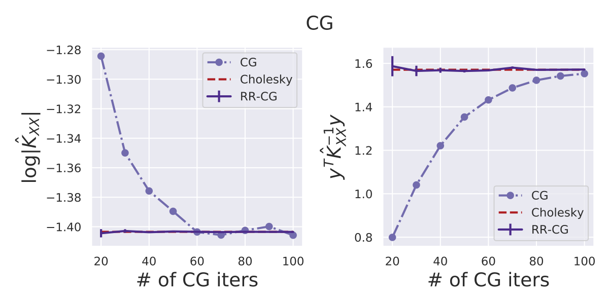
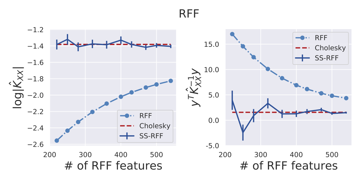
Figure 1: CG (left) systematically overestimates $\log|\widehat{\mathbf{K}}_{\mathbf{X}\mathbf{X}}|$ and underestimates $\mathbf{y}^{\top}\widehat{\mathbf{K}}_{\mathbf{X}\mathbf{X}}^{-1}\mathbf{y}$ whereas RFF (right) does the opposite. The dashed orange line shows the exact values computed by Cholesky. Our unbiased methods, RR-CG (left) and SS-RFF (right), recover the true $\log|\widehat{\mathbf{K}}_{\mathbf{X}\mathbf{X}}|$ and $\mathbf{y}^{\top}\widehat{\mathbf{K}}_{\mathbf{X}\mathbf{X}}^{-1}\mathbf{y}$ values. For these two methods, the $x$-axis indicates the expected number of iterations/features.

2.3 Unbiased Randomized Truncation

We will now briefly introduce Randomized Truncation Estimators, which are the primary tool we use to unbias the CG and RFF log marginal likelihood estimates. At a high level, assume that we wish to estimate some quantity $\psi$ that can be expressed as a (potentially-infinite) series:

$$\textstyle\psi=\sum_{j=1}^{H}\Delta_{j},\quad H\in\mathbb{N}\cup\{\infty\}.$$

Here and in the following sections, $\Delta_{j}$ can either be random or deterministic. To avoid the expensive evaluation of the full summation, a randomized truncation estimator chooses a random term $J\in\{1,\ldots,H\}$ with probability mass function $\mathbb{P}(J)=\mathbb{P}(\mathcal{J}=J)$ after which to truncate computation. In the following, we introduce two means of deriving unbiased estimators by upweighting the summation terms.

The Russian Roulette estimator (Kahn, 1955) obtains an unbiased estimator $\bar{\psi}_{J}$ by truncating the sum after $J\sim\mathbb{P}(J)$ terms and dividing the surviving terms by their survival probabilities:

$$\bar{\psi}_{J}=\sum_{j=1}^{J}\frac{\Delta_{j}}{\mathbb{P}(\mathcal{J}\geq j)}=\sum_{j=1}^{H}\left(\frac{\mathbb{I}_{J\geq j}}{\mathbb{P}(\mathcal{J}\geq j)}\right)\Delta_{j},$$ (6)

and, $\mathbb{E}[\bar{\boldsymbol{\psi}}_{J}]=\sum_{i=1}^{H}\Delta_{j}=\psi.$ (See appendix for further derivation.) The choice of $\mathbb{P}(J)$ determines both the computational efficiency and the variance of $\bar{\psi}_{J}$. A thin-tailed $\mathbb{P}(J)$ will often truncate sums after only a few terms ($J\ll H$). However, tail events $(J\approx H)$ are upweighted inversely to their low survival probability, and so thin-tailed truncation distributions may lead to high variance.

The Single Sample estimator (Lyne et al., 2015) implements an alternative reweighting scheme. After drawing $J\sim\mathbb{P}(J)$, it computes a single summation term $\Delta_{J}$, which it upweights by $1/\mathbb{P}(J)$:

$$\bar{\psi}_{J}=\frac{\Delta_{J}}{\mathbb{P}(J)}=\sum_{j=1}^{H}\left(\frac{\mathbb{I}_{J=j}}{\mathbb{P}(\mathcal{J}=j)}\right)\Delta_{j}.$$ (7)

This procedure is unbiased, and it amounts to estimating $\psi$ using a single importance-weighted sample from $\mathbb{P}(J)$ (see appendix). Again, $\mathbb{P}(J)$ controls the speed/variance trade-off. We refer the reader to (Beatson & Adams, 2019) for a detailed comparison of these two estimators. We emphasize that both estimators remain unbiased even if $\Delta_{j}$ is a random variable, as long as it is independent from the random truncation integer $J$.

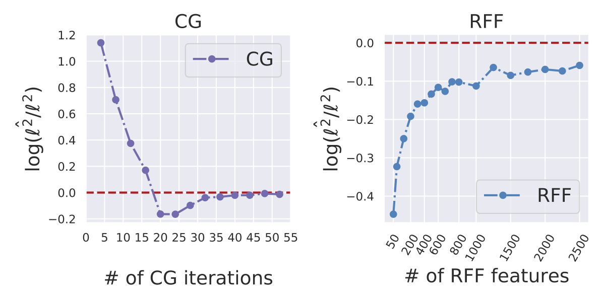
Figure 2: Kernel lengthscale values learned by optimizing (biased) CG and RFF log marginal likelihood approximations. CG overestimates the optimal kernel lengthscale whereas RFF underestimates it. We plot the divergence (in log-ratio scale) between the learned and true lengthscales as a function of the number of CG iterations (left) and of the number of RFF samples (right).

3 GP Learning with CG and RFF is Biased

Here we prove that early truncated CG and RFF provide biased approximations to the terms comprising the GP log marginal likelihood (Eq. 1). We also derive the bias decay rates for each method. We then empirically demonstrate these biases and show they affect the hyperparameters learned through optimization. Remarkably, we find that the above biases are highly systematic: CG-based GP learning favors underfitting hyperparameters while RFF-based learning favors overfitting hyperparameters.

3.1 CG Biases GP Towards Underfitting

In the GP literature, CG has often been considered an “exact” method for computing the log marginal likelihood (Cunningham et al., 2008; Cutajar et al., 2016), as the iterations are only truncated after reaching a pre-specified residual error threshold (e.g. $10^{-10}$). However, as CG is applied to ever-larger kernel matrices it is common to truncate the CG iterations before reaching this convergence (Wang et al., 2019). While this accelerates the hyperparameter learning process, the resulting solves and gradients can no longer be considered “exact.” In what follows, we show that the early-truncated CG optimization objective is not only approximate but also systematically biased towards underfitting.

To analyze the early-truncation bias, we adopt the analysis of Gardner et al. (2018) that recovers the GP log marginal likelihood (Eq. 1) from the stochastic gradient’s CG estimates of $\widehat{\mathbf{K}}_{\mathbf{X}\mathbf{X}}^{-1}\mathbf{y}$ and $\widehat{\mathbf{K}}_{\mathbf{X}\mathbf{X}}^{-1}\mathbf{z}$ (Eq. 3). Recall the two terms in the log marginal likelihood are the “data fit” term $\mathbf{y}^{\top}\widehat{\mathbf{K}}_{\mathbf{X}\mathbf{X}}^{-1}\mathbf{y}$ and the “model complexity” term $\log|\widehat{\mathbf{K}}_{\mathbf{X}\mathbf{X}}|$. The first term falls directly out of the CG estimate of $\widehat{\mathbf{K}}_{\mathbf{X}\mathbf{X}}^{-1}\mathbf{y}$, while a stochastic estimate of $\log|\widehat{\mathbf{K}}_{\mathbf{X}\mathbf{X}}|$ can be obtained through the byproducts of CG’s computation for $\widehat{\mathbf{K}}_{\mathbf{X}\mathbf{X}}^{-1}\mathbf{z}$. Gardner et al. (2018) show that the CG coefficients in Eq. 4 can be manipulated to produce a partial tridiagonalization: $\mathbf{T}^{(J)}_{\mathbf{z}}=\mathbf{Q}^{(J)\top}_{\mathbf{z}}\widehat{\mathbf{K}}_{\mathbf{X}\mathbf{X}}\mathbf{Q}^{(J)}_{\mathbf{z}},$ where $\mathbf{T}^{(J)}_{\mathbf{z}}\in\mathbb{R}^{J\times J}$ is tridiagonal. $\mathbf{T}^{(J)}_{\mathbf{z}}$ can compute the Stochastic Lanczos Quadrature estimate of $\widehat{\mathbf{K}}_{\mathbf{X}\mathbf{X}}$ (Ubaru et al., 2017; Dong et al., 2017):

$$\log|\widehat{\mathbf{K}}_{\mathbf{X}\mathbf{X}}| =\mathbb{E}\left[\mathbf{z}^{T}(\log\widehat{\mathbf{K}}_{\mathbf{X}\mathbf{X}})\mathbf{z}\right]$$

$$\approx\|\mathbf{z}\|^{2}\mathbf{e}_{1}^{\top}\left(\log\mathbf{T}_{\mathbf{z}}^{(J)}\right)\mathbf{e}_{1},$$ (8)

where $\log(\cdot)$ is the matrix logarithm and $\mathbf{e}_{1}$ is the first row of the identity matrix. The following theorem analyzes the bias of these $\mathbf{y}^{\top}\widehat{\mathbf{K}}_{\mathbf{X}\mathbf{X}}^{-1}\mathbf{y}$ and $\log|\widehat{\mathbf{K}}_{\mathbf{X}\mathbf{X}}|$ estimates:

Theorem 1.

Let $u_{J}$ and $v_{J}$ be the estimates of $\mathbf{y}^{\top}\widehat{\mathbf{K}}_{\mathbf{X}\mathbf{X}}^{-1}\mathbf{y}$ and $\log|\widehat{\mathbf{K}}_{\mathbf{X}\mathbf{X}}|$ respectively after $J$ iterations of CG; i.e.:

$$u_{J}=\mathbf{y}^{\top}\left({\textstyle\sum_{i=1}^{J}}\gamma_{i}\mathbf{d}_{i}\right),\quad v_{J}=\|\mathbf{z}\|^{2}\mathbf{e}_{1}^{\top}\left(\log\mathbf{T}_{\mathbf{z}}^{(J)}\right)\mathbf{e}_{1}.$$

If $J<N$, CG underestimates the inverse quadratic term and overestimates the log determinant in expectation:

$$u_{J}\leq\mathbf{y}^{\top}\widehat{\mathbf{K}}_{\mathbf{X}\mathbf{X}}^{-1}\mathbf{y},\quad\mathbb{E}_{\mathbf{z}}[v_{J}]\geq\log|\widehat{\mathbf{K}}_{\mathbf{X}\mathbf{X}}|.$$ (9)

The biases of both terms decay at a rate of $\mathchoice{\mathcal{O}\!\left(C^{-2J}\right)}{\mathcal{O}(C^{-2J})}{\mathcal{O}(C^{-2J})}{\mathcal{O}(C^{-2J})}$, where $C$ is a constant that depends on the conditioning of $\widehat{\mathbf{K}}_{\mathbf{X}\mathbf{X}}$.

Proof sketch. The direction of the biases can be proved using a connection between CG and numeric quadrature. $u_{J}$ and $v_{J}$ are exactly equal to the $J$-point Gauss quadrature approximation of $\mathbf{y}^{\top}\widehat{\mathbf{K}}_{\mathbf{X}\mathbf{X}}^{-1}\mathbf{y}$ and $\|\mathbf{z}\|^{2}\mathbf{e}_{1}^{\top}(\log\mathbf{T}^{(N)}_{\mathbf{z}})\mathbf{e}_{1}$ represented as Riemann-Stieltjes integrals. The sign of the CG approximation bias follows from the standard Gauss quadrature error bound, which is negative for $\mathbf{y}^{\top}\widehat{\mathbf{K}}_{\mathbf{X}\mathbf{X}}^{-1}\mathbf{y}$ and positive for $\log|\widehat{\mathbf{K}}_{\mathbf{X}\mathbf{X}}|$. The convergence rates are from standard bounds on CG (Golub & Van Loan, 2012) and the analysis of Ubaru et al. (2017). See appendix for a full proof.

Fig. 1 confirms our theoretical analysis and demonstrates the systematic biases of CG. We plot the log marginal likelihood terms for a subset of the PoleTele UCI dataset, varying the number of CG iterations ($J$) used to produce the estimates. Compared against the exact terms (computed with Cholesky), we see an overestimation of $\log|\widehat{\mathbf{K}}_{\mathbf{X}\mathbf{X}}|$ and an underestimation of $\mathbf{y}^{\top}\widehat{\mathbf{K}}_{\mathbf{X}\mathbf{X}}^{-1}\mathbf{y}$. These biases are most prominent when using few CG iterations.

We turn to study the effect of CG learning on hyperparameters. Since the log marginal likelihood is a nonconvex function of $\boldsymbol{\theta}$, it is not possible to directly prove how the bias affects $\boldsymbol{\theta}$. Nevertheless, we know intuitively that underestimating $\mathbf{y}^{\top}\widehat{\mathbf{K}}_{\mathbf{X}\mathbf{X}}^{-1}\mathbf{y}$ de-prioritizes model fit while overestimating $\log|\widehat{\mathbf{K}}_{\mathbf{X}\mathbf{X}}|$ over-penalizes model complexity. Thus, the learned hyperparameters will likely underfit the data. Underfitting may manifest in an overestimation of the learned lengthscale $\ell$, as low values of $\ell$ increase the flexibility and the complexity of the model. This hypothesis is empirically confirmed in Fig. 2 (left panel). We train a GP regression model on a toy dataset: $y=x\sin(5\pi x)+\varepsilon$ and $\varepsilon\sim\mathcal{N}(0,0.01)$. We fix all hyperparameters other than the lengthscale, which is learned using both CG-based optimization and (exact) Cholesky-based optimization. The overestimation of $\ell$ decays with the number of CG iterations.

3.2 RFF Biases GP Towards Overfitting

Previous work has studied the accuracy of RFF’s approximation to the entries of the Gram matrix $k(\mathbf{x},\mathbf{x}^{\prime})\approx\boldsymbol{\phi}(\mathbf{x})^{\top}\boldsymbol{\phi}(\mathbf{x}^{\prime})$ (Rahimi & Recht, 2008; Sutherland & Schneider, 2015). However, to the best of our knowledge there has been little analysis of nonlinear functions of this approximate Gram matrix, such as $\mathbf{y}^{\top}\widehat{\mathbf{K}}_{\mathbf{X}\mathbf{X}}^{-1}\mathbf{y}$ and $\log|\widehat{\mathbf{K}}_{\mathbf{X}\mathbf{X}}|$ appearing in the GP objective. Interestingly, we find that RFF systematically biases these terms:

Theorem 2.

Let $\widetilde{\mathbf{K}}_{J}$ be the RFF approximation with $J/2$ random features. In expectation, $\widetilde{\mathbf{K}}_{J}$ overestimates the inverse quadratic and underestimates the log determinant:

$${\textstyle\operatorname*{\mathbb{E}}_{\mathbb{P}(\boldsymbol{\omega})}\left[\mathbf{y}^{\top}\widetilde{\mathbf{K}}_{J}^{-1}\mathbf{y}\right]}\geq\mathbf{y}^{\top}\widehat{\mathbf{K}}_{\mathbf{X}\mathbf{X}}^{-1}\mathbf{y}$$ (10)

$${\textstyle\operatorname*{\mathbb{E}}_{\mathbb{P}(\boldsymbol{\omega})}\left[\log|\widetilde{\mathbf{K}}_{J}|\right]}\leq\log|\widehat{\mathbf{K}}_{\mathbf{X}\mathbf{X}}|.$$ (11)

The biases of both terms decay at a rate of $\mathchoice{\mathcal{O}\!\left(1/J\right)}{\mathcal{O}(1/J)}{\mathcal{O}(1/J)}{\mathcal{O}(1/J)}$.

Proof sketch. The direction of the biases is a straightforward application of Jensen’s inequality, noting that $\widehat{\mathbf{K}}_{\mathbf{X}\mathbf{X}}^{-1}$ is a convex function and $\log|\widehat{\mathbf{K}}_{\mathbf{X}\mathbf{X}}|$ is a concave function. The magnitude of the bias is derived from a second-order Taylor expansion that closely resembles the analysis of Nowozin (2018). See appendix for full proof.

Again, Fig. 1 confirms the systematic biases of RFF, which decay at a rate proportional to the number of features, as predicted by Thm. 2. Hence, RFF should affect the learned hyperparameters in a manner opposite to CG. Overestimating $\mathbf{y}^{\top}\widehat{\mathbf{K}}_{\mathbf{X}\mathbf{X}}^{-1}\mathbf{y}$ emphasizes data fitting while underestimating $\log|\widehat{\mathbf{K}}_{\mathbf{X}\mathbf{X}}|$ reduces the model complexity penalty, overall resulting in overfitting behavior. Following the intuition presented in Sec. 3.1, we expect the lengthscale to be underestimated, as empirically confirmed by Fig. 2 (right panel). The figure also illustrates the slow decay of the RFF bias.

4 Bias-free Scalable Gaussian Processes

We debias the estimates of both the GP training objective in Eq. 1 and its gradient in Eq. 2 (as approximated by CG and RFF) using unbiased randomized truncation estimators. To see how such estimators apply to GP hyperparameter learning, we note that both CG and RFF recover the true log marginal likelihood (or an unbiased estimate thereof) in their limits:

Observation 1.

CG recovers the exact log marginal likelihood in expectation in at most $N$ iterations:

$$\mathbf{y}^{\top}\widehat{\mathbf{K}}_{\mathbf{X}\mathbf{X}}^{-1}\mathbf{y} =\mathbf{y}^{\top}\left(\textstyle{\sum_{j=1}^{N}}\gamma_{j}\mathbf{d}_{j}\right),$$ (12)

$$\log|\widehat{\mathbf{K}}_{\mathbf{X}\mathbf{X}}| ={\textstyle\operatorname*{\mathbb{E}}_{\mathbf{z}}\left[\|\mathbf{z}\|^{2}\mathbf{e}_{1}^{\top}(\log\mathbf{T}^{(N)}_{\mathbf{z}})\mathbf{e}_{1}\right]}.$$ (13)

By the law of large numbers, RFF converges almost surely to the exact log marginal likelihood as the number of random features goes to infinity:

$$\mathbf{y}^{\top}\widehat{\mathbf{K}}_{\mathbf{X}\mathbf{X}}^{-1}\mathbf{y} =\lim_{J\to\infty}\mathbf{y}^{\top}\widetilde{\mathbf{K}}_{J}^{-1}\mathbf{y},$$ (14)

$$\log|\widehat{\mathbf{K}}_{\mathbf{X}\mathbf{X}}| =\lim_{J\to\infty}\log|\widetilde{\mathbf{K}}_{J}|.$$ (15)

To maintain the scalability of CG and RFFs while eliminating bias, we express the log marginal likelihood terms in Eqs. 12, 13, 14 and 15 as summations amenable to randomized truncation. We then apply the Russian Roulette and Single Sample estimators of Sec. 2.3 to avoid computing all summation terms while obtaining the same result in expectation.

4.1 Russian Roulette-Truncated CG (RR-CG)

The stochastic gradient in Eq. 3 requires performing two solves: $\widehat{\mathbf{K}}_{\mathbf{X}\mathbf{X}}^{-1}\mathbf{y}$ and $\widehat{\mathbf{K}}_{\mathbf{X}\mathbf{X}}^{-1}\mathbf{z}$. Using the summation formulation of CG (Eq. 4), we can write these two solves as series:

$$\textstyle\widehat{\mathbf{K}}_{\mathbf{X}\mathbf{X}}^{-1}\mathbf{y}=\sum_{i=1}^{N}\gamma_{i}\mathbf{d}_{i},\quad\widehat{\mathbf{K}}_{\mathbf{X}\mathbf{X}}^{-1}\mathbf{z}=\sum_{i=1}^{N}\gamma_{i}^{\prime}\mathbf{d}_{i}^{\prime},$$

where each CG iteration computes a new term of the summation. By applying the Russian Roulette estimator from Eq. 6, we obtain the following unbiased estimates:

$$\textstyle\begin{split}\textstyle\widehat{\mathbf{K}}_{\mathbf{X}\mathbf{X}}^{-1}\mathbf{y}&\approx{\textstyle\sum_{j=1}^{J}}(\gamma_{j}\mathbf{d}_{j})/\mathbb{P}(\mathcal{J}\geq j),\quad J\sim\mathbb{P}(J)\\ \textstyle\widehat{\mathbf{K}}_{\mathbf{X}\mathbf{X}}^{-1}\mathbf{z}&\approx{\textstyle\sum_{j=1}^{J^{\prime}}}(\gamma_{j}^{\prime}\mathbf{d}_{j}^{\prime})/\mathbb{P}(\mathcal{J}\geq j).\quad J^{\prime}\sim\mathbb{P}(J^{\prime}),\end{split}$$ (16)

These unbiased solves produce an unbiased optimization gradient in Eq. 3; we refer to this approach as Russian Roulette CG (RR-CG). With the appropriate truncation distribution $\mathbb{P}(J)$, this estimate affords the same computational complexity of standard CG without its bias.

We must compute two independent estimates of $\widehat{\mathbf{K}}_{\mathbf{X}\mathbf{X}}^{-1}\mathbf{y}$ with different $J\sim\mathbb{P}(J)$ in order for the $\mathbf{y}^{\top}\widehat{\mathbf{K}}_{\mathbf{X}\mathbf{X}}^{-1}\frac{\partial\widehat{\mathbf{K}}_{\mathbf{X}\mathbf{X}}}{\partial\boldsymbol{\theta}}\widehat{\mathbf{K}}_{\mathbf{X}\mathbf{X}}^{-1}\mathbf{y}$ term in Eq. 3 to be unbiased. Thus, the unbiased gradient requires 3 calls to RR-CG, as opposed to the 2 CG calls needed for the biased gradient. Nevertheless, RR-CG has the same $\mathchoice{\mathcal{O}\!\left(JN^{2}\right)}{\mathcal{O}(JN^{2})}{\mathcal{O}(JN^{2})}{\mathcal{O}(JN^{2})}$ complexity as standard CG – and the additional solve can be computed in parallel with the others.

We can also use the Russian Roulette estimator to compute the log marginal likelihood itself, though this is not strictly necessary for gradient-based optimization. (See appendix.)

Choosing the truncation distribution.

Since the Russian Roulette estimator is unbiased for any choice of $\mathbb{P}\left(J\right)$, we wish to choose a truncation distribution that balances computational cost and variance. Beatson & Adams (2019) propose the relative optimization efficiency (ROE) metric, which is the ratio of the expected improvement of taking an optimization step with our gradient estimate to its computational cost. A critical requirement of the ROE analysis is the expected rate of decay of our approximations in terms of the number of CG iterations $J$. We summarize our estimates and choices of distribution as follows:

Theorem 3.

The approximation to $\log|\widehat{\mathbf{K}}_{\mathbf{X}\mathbf{X}}|$ and to $\mathbf{y}^{\top}\widehat{\mathbf{K}}_{\mathbf{X}\mathbf{X}}^{-1}\mathbf{y}$ using RR-CG decays at a rate of $\mathchoice{\mathcal{O}\!\left(C^{-2J}\right)}{\mathcal{O}(C^{-2J})}{\mathcal{O}(C^{-2J})}{\mathcal{O}(C^{-2J})}$. Therefore the truncation distribution that maximizes the ROE is $\mathbb{P}^{*}(J)\propto C^{-2J}$, where $C$ is a constant that depends on the conditioning of $\widehat{\mathbf{K}}_{\mathbf{X}\mathbf{X}}$. The expected computation and variance of $\mathbb{P}^{*}\left(J\right)$ is finite.

Proof sketch. Beatson & Adams (2019) show that the truncation distribution that maximizes the ROE is proportional to the rate of decay of our approximation divided by its computational cost. The error of CG decays as $\mathchoice{\mathcal{O}\!\left(C^{-2J}\right)}{\mathcal{O}(C^{-2J})}{\mathcal{O}(C^{-2J})}{\mathcal{O}(C^{-2J})}$, and the cost of each summation term is constant with respect to $J$. In practice, we vary the exponential decaying rate to control the expectation and variance of $\mathbb{P}(J)$. To further reduce the variance of our estimator, we set a minimum number of CG iterations to be computed, as in (Luo et al., 2020). See appendix for full proof.

In practice, however, we do not have access to $C$ since computing the conditioning of $\widehat{\mathbf{K}}_{\mathbf{X}\mathbf{X}}$ is impractical. Yet, we can change the base of the exponential to $e$ and add a temperature parameter $\lambda$ to rescale the function and control the rate of decay of the truncation distribution as a sensible alternative. Thus, we follow a more general exponential decay distribution:

$$\mathbb{P}(J) \propto e^{-\lambda J},\qquad J=J_{\min},\cdots,N$$ (17)

where $J_{\min}$ is the minimum truncation number. By varying the values of $\lambda$ and $J_{\min}$, we can control the expectation and standard deviation of $\mathbb{P}(J)$. In practice we found that having the standard deviation value between 10 and 20 achieves stable GP learning process, which can be obtained by tuning $\lambda$ between $0.05$ and $0.1$ for sufficiently large datasets (e.g. $N\geq 500$). We also noticed that the method is not sensitive to these choices of hyperparameters and that they work well across all the experiments. The expected truncation number can be further tuned by varying $J_{\min}$. We emphasize that these choices impact the speed-variance tradeoff. By setting a larger $J_{\min}$ we decrease the speed by requiring more baseline computations but also decrease the variance (since the minimum approximations have the largest deviations from the ground truth).

Toy problem.

In Fig. 1 we plot the empirical mean of the RR-CG estimator using $10^{4}$ samples from an exponential truncation distribution. We find that RR-CG produces unbiased estimates of the $\mathbf{y}^{\top}\widehat{\mathbf{K}}_{\mathbf{X}\mathbf{X}}^{-1}\mathbf{y}$ and $\log|\widehat{\mathbf{K}}_{\mathbf{X}\mathbf{X}}|$ terms that are indistinguishable from the exact values computed with Cholesky. Reducing the expected truncation iteration $\mathbb{E}(J)$ (x-axis) increases the standard error of empirical means, demonstrating the speed-variance trade-off.

4.2 Single Sample-Truncated RFF (SS-RFF)

Denoting $\widetilde{}\mathbf{K}_{j}$ as the kernel matrix estimated by $j$ random Fourier features, we can write $\log|\widehat{\mathbf{K}}_{\mathbf{X}\mathbf{X}}|$ as the following telescoping series:

$$\log|\widehat{\mathbf{K}}_{\mathbf{X}\mathbf{X}}| ={\log|\widetilde{}\mathbf{K}_{1}|+\sum_{j=2}^{N/2-1}\left(\log|\widetilde{}\mathbf{K}_{j}|-\log|\widetilde{}\mathbf{K}_{j-1}|\right)}$$ (18)

$$+\log|\widehat{\mathbf{K}}_{\mathbf{X}\mathbf{X}}|-\log|\widetilde{}\mathbf{K}_{N/2-1}|$$

$$={\textstyle\log|\widetilde{}\mathbf{K}_{1}|+\sum_{j=2}^{N/2}\Delta_{j},}$$ (19)

where $\Delta_{j}$ is defined as $\log|\widetilde{}\mathbf{K}_{j}|-\log|\widetilde{}\mathbf{K}_{j-1}|$ for all $j<N/2$, and $\Delta_{N/2}$ is defined as $\log|\widehat{\mathbf{K}}_{\mathbf{X}\mathbf{X}}|-\log|\widetilde{}\mathbf{K}_{N/2-1}|$. Note that each $\Delta_{j}$ is now a random variable, since it depends on the random Fourier frequencies $\omega$. Crucially, we only include $N/2$ terms in the series so that no term requires more than $\mathchoice{\mathcal{O}\!\left(N^{3}\right)}{\mathcal{O}(N^{3})}{\mathcal{O}(N^{3})}{\mathcal{O}(N^{3})}$ computation in expectation. (For any $j>N/2$, $\widetilde{}\mathbf{K}_{j}$ is a full-rank matrix and thus is as computationally expensive as the true $\widehat{\mathbf{K}}_{\mathbf{X}\mathbf{X}}$ matrix.) We construct a similar telescoping series for $\mathbf{y}^{\top}\widehat{\mathbf{K}}_{\mathbf{X}\mathbf{X}}^{-1}\mathbf{y}$.

As with Eq. 16, we approximate the series in Eq. 19 with a randomized truncation estimator, this time using the Single Sample estimator (7):

$$\log|\widehat{\mathbf{K}}_{\mathbf{X}\mathbf{X}}|\approx\log|\widetilde{}\mathbf{K}_{1}|+\Delta_{J}/\mathbb{P}\left(J\right).$$ (20)

where $J$ is drawn from the truncation distribution $\mathbb{P}(J)$ with support over $\{2,3,\ldots N/2\}$. Note that the Single Sample estimate requires computing 3 log determinants ($\log|\widetilde{}\mathbf{K}_{1}|$, $\log|\widetilde{}\mathbf{K}_{J-1}|$, and $\log|\widetilde{}\mathbf{K}_{J}|$) for a total of $\mathchoice{\mathcal{O}\!\left(J^{3}+NJ^{2}\right)}{\mathcal{O}(J^{3}+NJ^{2})}{\mathcal{O}(J^{3}+NJ^{2})}{\mathcal{O}(J^{3}+NJ^{2})}$ computations and $\mathchoice{\mathcal{O}\!\left(NJ\right)}{\mathcal{O}(NJ)}{\mathcal{O}(NJ)}{\mathcal{O}(NJ)}$ memory. This is asymptotically the same requirement as standard RFF. The Russian Roulette estimator, on the other hand, incurs a computational cost of $\mathchoice{\mathcal{O}\!\left(NJ^{3}+J^{4}\right)}{\mathcal{O}(NJ^{3}+J^{4})}{\mathcal{O}(NJ^{3}+J^{4})}{\mathcal{O}(NJ^{3}+J^{4})}$ as it requires computing ($\log|\widetilde{}\mathbf{K}_{1}|$ through $\log|\widetilde{}\mathbf{K}_{J}|$) which quickly becomes impractical for large $J$.

A similar Single Sample estimator constructs an unbiased estimate of $\mathbf{y}^{\top}\widehat{\mathbf{K}}_{\mathbf{X}\mathbf{X}}^{-1}\mathbf{y}$. Backpropagating through these Single Sample estimates produces unbiased estimates of the log marginal likelihood gradient in Eq. 2.

Choosing the truncation distribution.

For the Single Sample estimator we do not have to optimize the ROE since minimizing the variance of this estimator does not result in a degenerate distribution.

Theorem 4.

The truncation distribution that minimizes the variance of the SS-RFF estimators for $\log|\widehat{\mathbf{K}}_{\mathbf{X}\mathbf{X}}|$ and $\mathbf{y}^{\top}\widehat{\mathbf{K}}_{\mathbf{X}\mathbf{X}}^{-1}\mathbf{y}$ is $\mathbb{P}^{*}\left(J\right)\propto 1/J$. The expected variance and computation of $\mathbb{P}^{*}(J)$ is finite.

Proof sketch. The minimum variance distribution can be found by solving a constrained optimization problem. In practice, we can further decrease the variance of our estimator by fixing a minimum value of RFF features to be used in Eq. 19 and by increasing the step size ($c\in\mathbb{N}$) between the elements at each $\Delta_{j}$ = $\log|\widetilde{\mathbf{K}}_{cJ}|-\log|\widetilde{\mathbf{K}}_{c(J-1)}|$. See appendix for full proof.

For the experiments we started with 500 features and also tried various step sizes $c\in\{1,10,100\}$. The variance of the estimator decreases as we increase $c$ since the probability weights will decrease in magnitude. Yet, despite of using the optimal truncation distribution, setting a high number of features and taking long steps $c=100$, the variance of the estimator still requires taking several steps before converging, making SS-RFF computationally impractical.

Toy problem.

Similar to RR-CG, in Fig. 1 we plot the empirical mean of the SS-RFF estimator using $10^{4}$ samples. We find that SS-RFF produces unbiased estimates of the $\mathbf{y}^{\top}\widehat{\mathbf{K}}_{\mathbf{X}\mathbf{X}}^{-1}\mathbf{y}$ and $\log|\widehat{\mathbf{K}}_{\mathbf{X}\mathbf{X}}|$ terms. However, these estimates have a higher variance when compared to the estimates of RR-CG. Reducing the expected truncation iteration $\mathbb{E}(J)$ (x-axis) increases the standard error of the empirical means, demonstrating the speed-variance trade-off.

4.3 Analysis of the Bias-free Methods

Randomized truncations and conjugate gradients have existed for many decades (Hestenes et al., 1952; Kahn, 1955), but have rarely been used in conjunction. Filippone & Engler (2015) proposed a method closely related to our RR-CG which performs randomized early-truncation of CG iterations to obtain unbiased posterior samples of the GP covariance parameters. We differ by tackling the GP hyperparameter learning problem: we provide the first theoretical analysis of the biases incurred by both CG and RFF, and proceed to tailor unbiased estimators for each method.

To some extent, randomized truncation methods are antithetical to the original intention of CG: producing deterministic and nearly exact solves. For large-scale applications, where early truncation is necessary for computational tractability, the ability to trade bias for variance is beneficial. This fact is especially true in the context of GP learning, where the bias of early truncation is systematic and cannot be simply explained away as numerical imprecision.

Randomized truncation estimates are often used to estimate infinite series, where it is challenging to design truncation distributions with finite expected computation and/or variance. We avoid such issues since CG and the telescoping RFF summations are both finite.

5 Results

First, we show that our bias-free methods recover nearly the same hyperparameters as exact methods (i.e. Cholesky-based optimization), whereas models that use CG and RFF converge to suboptimal hyperparameters. Since RR-CG and SS-RFF eliminate bias at the cost of increased variance, we then demonstrate the optimization convergence rate and draw conclusions on our methods’ applicability. Finally, we compare models optimized with RR-CG against a host of approximate GP methods across a wide range of UCI datasets (Asuncion & Newman, 2007). All experiments are implemented in GPyTorch (Gardner et al., 2018)

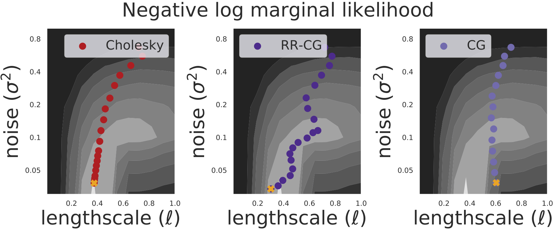
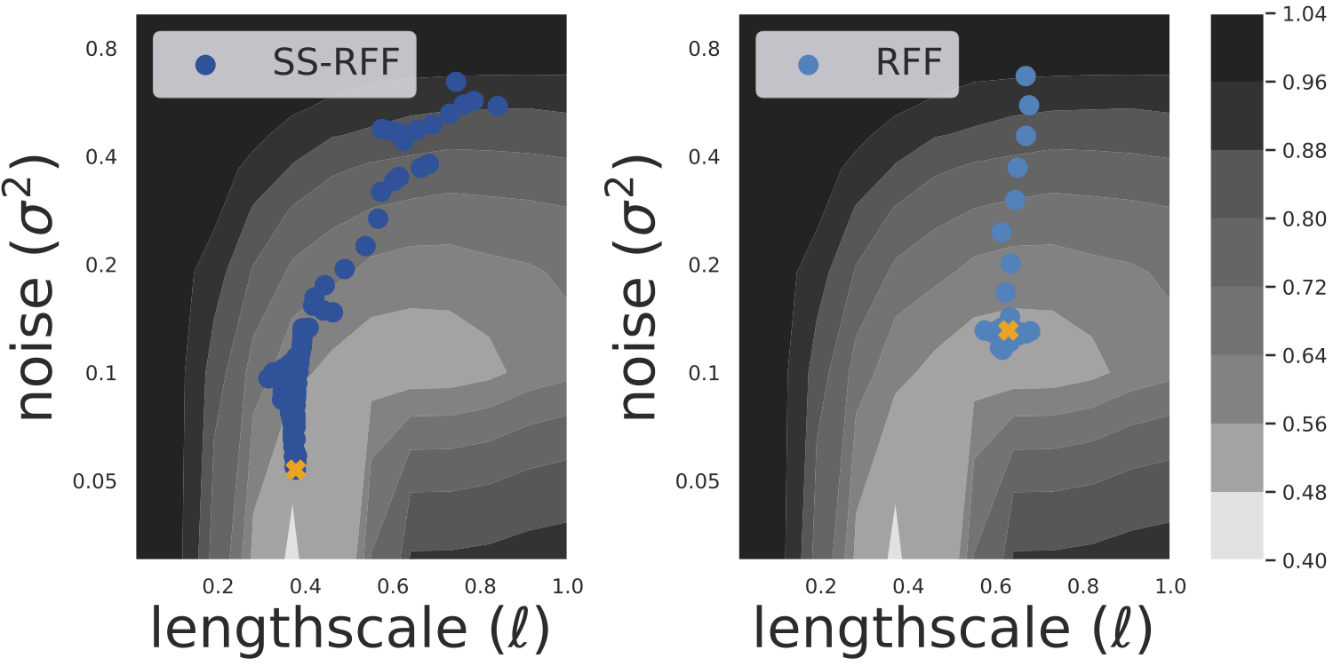
Figure 3: Optimization landscape of a GP with two hyperparameters. The SS-RFF and RR-CG models converge to similar hyperparameter values that are nearly optimal, while the RFF and CG models converge to suboptimal solutions. In addition, the stochastic effect of the randomized truncation is visible in the trajectories of RR-CG and SS-RFF. Moreover, CG (and RR-CG) models truncate after $20$ iterations (in expectation); RFF (and SS-RFF) models use $700$ features (in expectation).

Optimization trajectories of bias-free GP.

Fig. 3 displays the optimization landscape – the log marginal likelihood of the PoleTele dataset – as a function of (RBF) kernel lengthscale $\ell$ and noise $\sigma^{2}$. As expected, an exact GP (optimized using Cholesky, Fig. 3 upper left) recovers the optimum. Notably, the GP trained with standard CG and RFF converges to suboptimal hyperparameters (upper right/lower right). RR-CG and SS-RFF models (trained with 20 iterations and 700 features in expectation, respectively) successfully eliminate this bias, and recover nearly the same parameters as the exact model (upper center/lower left). These plots also show the speed-variance tradeoff of randomized truncation. SS-RFF and RR-CG have noisy optimization trajectories due to auxiliary truncation variance.

Convergence of GP hyperparameter optimization.

Figs. 5 and 4 plot the exact GP log marginal likelihood of the parameters learned by each method during optimization. Each trajectory corresponds to a RBF-kernel GP trained on the PoleTele dataset (Fig. 4) and the Bike dataset (Fig. 5).

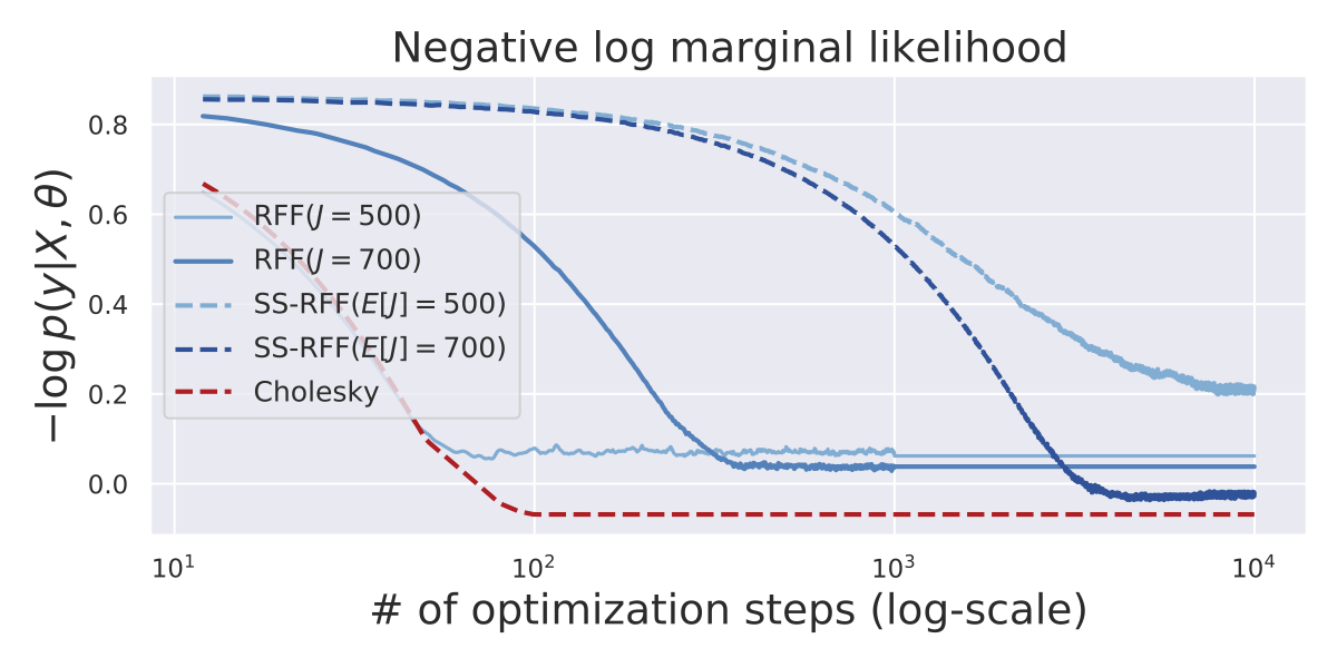
Figure 4: The GP optimization objective for models trained with RFF and SS-RFF. (PoleTele dataset, RBF kernel, Adam optimizer.) RFF models converge to sub-optimal log marginal likelihoods. SS-RFF models converge to (near) optimum values, yet require more than $100\times$ as many optimization steps.

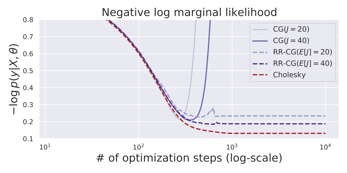
Figure 5: The GP optimization objective for models trained with CG and RR-CG. (Bike dataset, RBF kernel, Adam optimizer.) RR-CG models converge to optimal solutions, while the (biased) CG models diverge. Increasing the expected truncation of RR-CG only slightly improves optimization convergence; models converge in $<100$ steps of Adam.

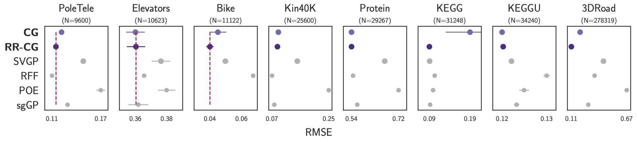
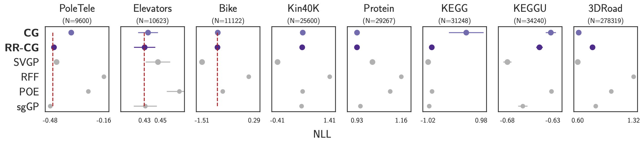
Figure 6: Root-mean-square-error (RMSE) and negative log likelihood (NLL) of GP trained with CG (light purple), RR-CG (dark purple) and various approximate methods (grey). Dashed red lines indicates Cholesky-based GP performance (when applicable). Results are averaged over 3 dataset splits. Missing RFF and sgGP results correspond to (very high) outlier NLL / RMSE values. In almost all experiments, GP learning with RR-CG achieves similar or better performance compared to that with CG at the same computational cost.

Fig. 4 shows that RFF models converge to solutions with worse log likelihoods, and more RFF features slow the rate of optimization. Additionally, we see the cost of the auxiliary variance needed to debias SS-RFF: while SS-RFF models achieve better optima than their biased counterparts, they take 2-3 orders of magnitude longer to converge, despite using a truncation distribution that minimizes variance. We thus conclude that SS-RFF has too much variance to be practical for GP hyperparameter learning.

Fig. 5 on the other hand shows that RR-CG is minimally affected by its auxiliary variance. The GP trained with RR-CG converges in roughly $100$ iterations, nearly matching Cholesky-based optimization. Decreasing the expected truncation value from $\mathbb{E}[J]=40$ to $20$ slightly slows this convergence. We note that the bias induced by standard CG can be especially detrimental to GP learning. On this dataset, the biased models deviate from their Cholesky counterparts and eventually diverge away from the optimum.

Predictive performance of bias-free GP.

Lastly, we compare the predictive performance of GPs that use RR-CG, CG, and Cholesky for hyperparameter optimization. We emphasize that the RR-CG and CG methods only make use of early truncation approximations during training. At test time, we compute the predictive posterior by running CG to a tolerance of $\leq 10^{-4}$, which we believe can be considered “exact” for practical intents and purposes. Additionally, we include four other (biased) scalable GP approximations methods as baselines: RFF, Stochastic Variational Gaussian Processes (SVGP) (Hensman et al., 2013), generalized Product of Expert Gaussian Processes (POE) (Cao & Fleet, 2014; Deisenroth & Ng, 2015), and stochastic gradient-based Gaussian Processes (sgGP) (Chen et al., 2020). We note that the RFF, SVGP, and sgGP methods introduce both bias and variance, as these methods rely on randomization and approximation.

We use CG with $J=100$ iterations, and RR-CG with $\mathbb{E}[J]=100$ expected iterations; both methods use the preconditioner of Gardner et al. (2018). All RFF models use $700$ random features. For SVGP, we use $1{,}024$ inducing points and minibatches of size $1{,}024$ as in (Wang et al., 2019). The POE models are comprised of GP experts that are each trained on $1{,}024$ data point subsets. For sgGP, the subsampled datasets are constructed by selecting a random point $\mathbf{x},y$ and its 15 nearest neighbors as in (Chen et al., 2020). Each dataset is randomly split to 64% training, 16% validation and 20% testing sets. All kernels are RBF with a separate lengthscale per dimension. See appendix for more details.

We report prediction accuracy (RMSE) and negative log likelihood (NLL) in Fig. 6 (see appendix for full tables on predictive performance and training time). We make two key observations: (i) RR-CG meaningfully debiases CG. When the bias of CG is not detrimental to optimization (e.g. CG with 100 iterations is close to convergence for the Elevators dataset), RR-CG has similar performance. However, when the CG bias is more significant (e.g. the KEGG dataset), the bias-free RR-CG improves the GP predictive RMSE and NLL. We also include a figure displaying the predictive performance of RR-CG and CG with increasing number of (expected) CG iterations in appendix. (ii) RR-CG recovers the same optimum as the “ground-truth” method (i.e. Cholesky) does, as indicated by the red-dashed line in Fig. 6. This result provides additional evidence that RR-CG achieves unbiased optimization.

While RR-CG obtains the lowest RMSE on all but 2 datasets, we note that the (biased) GP approximations sometimes achieve lower NLL. For example, SVGP has a lower NLL than that of RR-CG on the Bike dataset, despite having a higher RMSE. We emphasize that this is not a failing of RR-CG inference. The SVGP NLL is even better than that of the exact (Cholesky) GP, suggesting a potential model misspecification for this particular dataset. Since SVGP overestimates the observational noise $\sigma^{2}$ (Bauer et al., 2016), it may obtain a better NLL when outliers are abundant. Though we cannot compare against the Cholesky posterior on larger datasets, we hypothesize that the NLL/RMSE discrepancy on these datasets is due to a similar modeling issue.

6 Conclusion

We prove that CG and RFF introduce systematic biases to the GP log marginal likelihood objective: CG-based training will favor underfitting models, while RFF-based training will promote overfitting. Modifying these methods with randomized truncation converts these biases into variance, enabling unbiased stochastic optimization. Our results show that this bias-to-variance exchange indeed constitutes a trade-off. The convergence of SS-RFF is impractically slow, likely due to the truncation variance needed to eliminate RFF’s slowly-decaying bias. However, for CG-based training, we find that variance is almost always preferable to bias. Models trained with RR-CG achieve better performance than those trained with standard CG, and tend to recover the hyperparameters learned with exact methods. Though models trained with CG do not always exhibit noticeable bias, RR-CG’s negligible computational overhead is justifiable to counteract cases where the bias is significant.

We reported experiments with at most 300K observations for our methods and baselines, which is substantial for GPs. We emphasize that RR-CG can be extended to datasets with over one million data points as in Wang et al. (2019). However, the computational cost is much higher, requiring multiple GPUs for training and testing.

We note that the RR-CG algorithm is not limited to GP applications. Future work should explore applying RR-CG to other optimization problems with large-scale solves.

Appendix A Proof of Biases for CG and RFF

A.1 Proof of Theorem 1

Proof.

To prove the bias of the CG log marginal likelihood terms, we rely on a connection between conjugate gradients, the Lanczos algorithm (Lanczos, 1950), and Gauss quadrature. In particular, we demonstrate that $u_{J}$ and $v_{J}$ – CG’s estimates for $\mathbf{y}^{\top}\widehat{\mathbf{K}}_{\mathbf{X}\mathbf{X}}^{-1}\mathbf{y}$ and $\log|\widehat{\mathbf{K}}_{\mathbf{X}\mathbf{X}}|$ terms – are equivalent to Gauss quadrature approximations of two Riemann-Stieljes integrals. We then use quadrature error analysis to prove the biases of these terms.

Expressing $\mathbf{y}^{\top}\widehat{\mathbf{K}}_{\mathbf{X}\mathbf{X}}^{-1}\mathbf{y}$ and $\mathbf{z}^{\top}(\log\widehat{\mathbf{K}}_{\mathbf{X}\mathbf{X}})\mathbf{z}$ as Riemann-Stieljes integrals.

First, we note that $\mathbf{y}^{\top}\widehat{\mathbf{K}}_{\mathbf{X}\mathbf{X}}^{-1}\mathbf{y}$ and $\mathbf{z}^{\top}(\log\widehat{\mathbf{K}}_{\mathbf{X}\mathbf{X}})\mathbf{z}$ (our stochastic trace estimate of $\log|\widehat{\mathbf{K}}_{\mathbf{X}\mathbf{X}}|$) can both be expressed by the quadratic form $\mathbf{w}^{\top}f(\mathbf{A})\mathbf{w}$, where $f(\mathbf{A})$ denotes a matrix function of the matrix $\mathbf{A}$, and $\mathbf{w}$ is a vector. Letting $\mathbf{A}=\mathbf{P}\boldsymbol{\Lambda}\mathbf{P}^{\top}$ be the eigendecomposition of $\mathbf{A}$, we can write this quadratic form as

$$\mathbf{w}^{\top}f(\mathbf{A})\mathbf{w} =\mathbf{w}^{\top}\mathbf{P}f(\boldsymbol{\Lambda})\mathbf{P}^{\top}\mathbf{w}=\|\mathbf{w}\|^{2}\sum_{i=1}^{N}f(\lambda_{i})\mu_{i}^{2},$$

where $\lambda_{\min}\leq\lambda_{i}\leq\lambda_{\max}$ are the diagonal elements of $\boldsymbol{\Lambda}$ (i.e. the eigenvalues) – ordered from smallest to largest, and $\mu_{i}$ are the components of $\mathbf{P}^{\top}\mathbf{w}/\|\mathbf{w}\|$. The summation in the above equation can be expressed as a Riemann-Stieltjes integral:

$$I[f] \vcentcolon=\|\mathbf{w}\|^{2}\sum_{i=1}^{N}f(\lambda_{i})\mu_{i}^{2}$$

$$=\|\mathbf{w}\|^{2}\int_{\lambda_{\min}}^{\lambda_{\max}}f(t)d\mu_{\mathbf{A}}(t),$$ (S1)

where the measure $\mu_{\mathbf{A}}(t)$ is a piecewise constant function

$$\mu_{\mathbf{A}}(t) =\begin{cases}0,\qquad&\textrm{if }t<\lambda_{\min},\\ \sum_{j=1}^{i}\mu_{j}^{2},\qquad&\textrm{if }\lambda_{i}\leq t<\lambda_{i-1}\\ \sum_{j=1}^{N}\mu_{j}^{2},\qquad&\textrm{if }\lambda_{\max}\leq t.\end{cases}$$ (S2)

See (Golub & Meurant, 2009) for more details.

The Lanczos algorithm approximates these integrals with Gauss quadrature.

The Lanczos algorithm (Lanczos, 1950), which is briefly described in Sec. 3.1, iteratively expresses a symmetric matrix $\mathbf{A}$ via the partial tridiagonalization $\mathbf{T}^{(J)}_{\mathbf{w}}=\mathbf{Q}^{(J)\top}_{\mathbf{w}}\mathbf{A}\mathbf{Q}^{(J)}_{\mathbf{w}}$. $\mathbf{Q}^{(J)}_{\mathbf{w}}\in\mathbb{R}^{N\times J}$ is a orthonormal matrix with $\mathbf{w}/\|\mathbf{w}\|$ as its first column, and $\mathbf{T}^{(J)}_{\mathbf{w}}$ is a $J\times J$ tridiagonal matrix. Briefly, the columns of $\mathbf{Q}^{(J)}$ matrices are computed by performing Gram-Schmidt orthogonalization on the Krylov subspace $[\mathbf{w},\mathbf{A}\mathbf{w},\mathbf{A}^{2}\mathbf{w},\ldots,\mathbf{A}^{J-1}\mathbf{w}]$, and storing the orthogonalization constants in $\mathbf{T}^{(J)}_{\mathbf{w}}$.

The Lanczos algorithm is commonly used to estimate quadratic forms:

$$\mathbf{w}^{\top}f(\mathbf{A})\mathbf{w} \approx\mathbf{w}^{\top}\mathbf{Q}^{(J)})_{\mathbf{w}}f\left(\mathbf{T}^{(J)}_{\mathbf{w}}\right)\mathbf{Q}^{(J)\top})_{\mathbf{w}}\mathbf{w}$$

$$=\|\mathbf{w}\|^{2}\mathbf{e}^{\top}_{1}f\left(\mathbf{T}^{(J)}_{\mathbf{w}}\right)\mathbf{e}_{1},$$ (S3)

where $\mathbf{e}_{1}$ is the first unit vector. Note that Eq. S3 holds because the columns of $\mathbf{Q}^{(J)}_{\mathbf{w}}$ are orthonormal.

There is a well-established connection between Eq. S3 and numeric quadrature (e.g. Golub & Meurant, 2009). More specifically, Eq. S3 is exactly equivalent to a $J$-term Gauss quadrature rule applied to the Riemann-Stieltjes integral in Eq. S1. We can thus analyze Lanczos estimates of $\mathbf{w}^{\top}f(\mathbf{A})\mathbf{w}$ using standard Gauss quadrature error analysis.

Equivalence between CG and the Lanczos algorithm.

We will now show an equivalence between our estimates $u_{J}\approx\mathbf{y}^{\top}\widehat{\mathbf{K}}_{\mathbf{X}\mathbf{X}}^{-1}\mathbf{y}$ and $v_{J}\approx\mathbf{z}^{\top}(\log\widehat{\mathbf{K}}_{\mathbf{X}\mathbf{X}})\mathbf{z}$ and Lanczos algorithm approximations. Note that we have already established $v_{J}\approx\mathbf{z}^{\top}(\log\widehat{\mathbf{K}}_{\mathbf{X}\mathbf{X}})\mathbf{z}$ as a Lanczos algorithm approximation in Sec. 3.1:

$$\mathbf{z}^{\top}=\|\mathbf{z}\|^{2}\mathbf{e}_{1}^{\top}(\log\mathbf{T}^{(J)}_{\mathbf{z}})\mathbf{e}_{1}.$$

For $u_{J}\approx\mathbf{y}^{\top}\widehat{\mathbf{K}}_{\mathbf{X}\mathbf{X}}^{-1}\mathbf{y}$, we exploit a connection between CG and Lanczos (Golub & Van Loan, 2012, Ch. 11.3):

$$\sum_{j=1}^{J}\gamma_{j}\mathbf{d}_{j}=\|\mathbf{y}\|\mathbf{Q}_{\mathbf{y}}^{(J)}(\mathbf{T}_{\mathbf{y}}^{(J)})^{-1}\mathbf{e}_{1},$$ (S4)

where $\sum_{j=1}^{J}\gamma_{j}\mathbf{d}_{j}$ (see Eq. 4) is the $J^{\text{th}}$ CG approximation to $\widehat{\mathbf{K}}_{\mathbf{X}\mathbf{X}}^{-1}\mathbf{y}$. Multiplying Eq. S4 by $\mathbf{y}^{\top}$, we have

$$u_{J} =\mathbf{y}^{\top}\left(\sum_{j=1}^{J}\gamma_{j}\mathbf{d}_{j}\right)$$

$$=\|\mathbf{y}\|\mathbf{y}^{\top}\mathbf{Q}_{\mathbf{y}}^{(J)}(\mathbf{T}_{\mathbf{y}}^{(J)})^{-1}\mathbf{e}_{1}$$

$$=\|\mathbf{y}\|^{2}\mathbf{e}_{1}^{\top}(\mathbf{T}_{\mathbf{y}}^{(J)})^{-1}\mathbf{e}.$$

Therefore, the CG approximations of $\mathbf{y}^{\top}\widehat{\mathbf{K}}_{\mathbf{X}\mathbf{X}}^{-1}\mathbf{y}$ and $\mathbf{z}^{\top}(\log\widehat{\mathbf{K}}_{\mathbf{X}\mathbf{X}})\mathbf{z}$ are both Lanczos approximations. Putting all the pieces together, we have just shown that $u_{J}$ and $v_{J}$ are equivalent to $J$-term Gauss quadrature rules applied to the following integrals:

$$\mathbf{y}^{\top}\widehat{\mathbf{K}}_{\mathbf{X}\mathbf{X}}^{-1}\mathbf{y} =\|\mathbf{y}\|^{2}\int_{\lambda_{\min}}^{\lambda_{\max}}t^{-1}\,\mathrm{d}{\mu}_{\widehat{\mathbf{K}}_{\mathbf{X}\mathbf{X}}}(t),$$ (S5)

$$\mathbf{z}^{\top}\left(\log\widehat{\mathbf{K}}_{\mathbf{X}\mathbf{X}}^{-1}\right)\mathbf{z} =\|\mathbf{z}\|^{2}\int_{\lambda_{\min}}^{\lambda_{\max}}\log(t)\,\mathrm{d}{\mu}_{\widehat{\mathbf{K}}_{\mathbf{X}\mathbf{X}}}(t),$$ (S6)

where the measure $\mu_{\widehat{\mathbf{K}}_{\mathbf{X}\mathbf{X}}}(t)$ is defined by Eq. S2.

Applying Gauss quadrature error analysis to $u_{J}$ and $v_{J}$.

To analyze the bias of teh CG estimates, we make use of standard error Guass quadrature error analysis. If $L_{G}^{(J)}[f]$ is the $J$-term Gaussian quadrature approximation of the Riemann-Stieltjes integral $I[f]$ (see Eq. S1), the error can be exactly expressed as:

$$I[f]-L_{G}^{(J)}[f] =(\gamma_{1}\cdots\gamma_{J-1})^{2}\frac{f^{(2J)}(\eta)}{(2J)\!},$$ (S7)

for some $\eta\in[\lambda_{\min},\lambda_{\max}]$, where $f^{(2J)}$ is the $2J^{\text{th}}$ derivative of $f$ and $\{\gamma_{i}\}$ are some quantities that depend on the spectrum of the matrix $\widehat{\mathbf{K}}_{\mathbf{X}\mathbf{X}}$ (Golub & Meurant, 2009, Ch. 6).

Turning back to $u_{J}$, the corresponding function $f(t)=t^{-1}$ has even derivatives of the form $f^{(2J)}=(2J)!\>t^{-(2J+1)}>0,\forall J,\forall t\in(\lambda_{\min},\lambda_{\max})$. Replacing $I[f]$ with the integral defined by Eq. S5, we have that $\mathbf{y}^{\top}\widehat{\mathbf{K}}_{\mathbf{X}\mathbf{X}}^{-1}\mathbf{y}-u_{J}\geq 0$, which proves that CG underestimates $\mathbf{y}^{\top}\widehat{\mathbf{K}}_{\mathbf{X}\mathbf{X}}^{-1}\mathbf{y}$. Similarly for $v_{J}$, the corresponding $f(t)=\log t$ has even derivatives of the form $f^{(2J)}=-(2J-1)!\>t^{-2J}<0,\forall J,\forall t\in(\lambda_{\min},\lambda_{\max})$. Replacing $I[f]$ with the integral defined by Eq. S6, we have that $\mathbf{z}^{\top}(\log\widehat{\mathbf{K}}_{\mathbf{X}\mathbf{X}})\mathbf{z}-v_{J}\leq 0$.

The convergence rates

of $u_{J}$ and $v_{J}$ follow from Eq. 4.4 of Ubaru et al. (2017). Let $\rho=(\sqrt{\kappa}+1)/(\sqrt{\kappa}-1)$, where $\kappa$ is the condition number of $\widehat{\mathbf{K}}_{\mathbf{X}\mathbf{X}}$ (i.e. the ratio of its maximum and minimum singular values). Then

$$\|\mathbf{y}^{\top}\widehat{\mathbf{K}}_{\mathbf{X}\mathbf{X}}^{-1}\mathbf{y}-u_{J}\| \leq C\rho^{-2J},$$

$$\|\mathbf{z}^{\top}(\log\widehat{\mathbf{K}}_{\mathbf{X}\mathbf{X}})\mathbf{z}-v_{J}\| \leq C\rho^{-2J},$$

where $C$ is a constant that depends on the extremal eigenvalues of $\widehat{\mathbf{K}}_{\mathbf{X}\mathbf{X}}$. ∎

A.2 Proof of Theorem 2

Proof.

The inequalities are a result of applying Jensen’s inequality to the inverse of a positive definite matrix (which is a convex function) and the log determinant of a positive definite matrix (which is a concave function). For example, for the $\mathbf{y}^{\top}\widehat{\mathbf{K}}_{\mathbf{X}\mathbf{X}}^{-1}\mathbf{y}$ term we have that

$$\begin{split}\operatorname*{\mathbb{E}}_{\mathbb{P}(\boldsymbol{\omega})}\left[\mathbf{y}^{\top}\widetilde{\mathbf{K}}_{J}^{-1}\mathbf{y}\right]&=\mathbf{y}^{\top}\operatorname*{\mathbb{E}}_{\mathbb{P}(\boldsymbol{\omega})}\left[\widetilde{\mathbf{K}}_{J}^{-1}\right]\mathbf{y}\\ &\geq\mathbf{y}^{\top}\left(\operatorname*{\mathbb{E}}_{\mathbb{P}(\boldsymbol{\omega})}\left[\widetilde{\mathbf{K}}_{J}\right]\right)^{-1}\mathbf{y}\\ &=\mathbf{y}^{\top}\widehat{\mathbf{K}}_{\mathbf{X}\mathbf{X}}^{-1}\mathbf{y}\\ \end{split}$$

A similar procedure, but in the opposite direction applies to the $\log|\widehat{\mathbf{K}}_{\mathbf{X}\mathbf{X}}|$.

To estimate the rate of decay of the biases, we rely on two keys ideas. The first idea is to translate the central moments of the kernel matrix being approximated by the random Fourier features into the central moments of these features. This strategy resembles the analysis in (Nowozin, 2018) which uses (Angelova, 2012, Theorem 1). The second idea is to use an approximation to two matrix functions. For the inverse function we use a Neumann series and for the logarithm we use a Taylor series. These series require that the eigenvalues of the approximation residual ($\widehat{\mathbf{K}}_{\mathbf{X}\mathbf{X}}-\widetilde{K}_{J})$ are less than 1. We will make this assumption as we know that for a large enough $J$, the kernel approximation will be close to $\widehat{\mathbf{K}}_{\mathbf{X}\mathbf{X}}$. Below is a formal argument.

For a fixed $\boldsymbol{\omega}$ we can write

$$\begin{split}&\mathbf{y}^{\top}\widetilde{\mathbf{K}}_{J}^{-1}\mathbf{y}=\mathbf{y}^{\top}\left(\widehat{\mathbf{K}}_{\mathbf{X}\mathbf{X}}-\widehat{\mathbf{K}}_{\mathbf{X}\mathbf{X}}+\widetilde{\mathbf{K}}_{J}\right)^{-1}\mathbf{y}\\ &=\mathbf{y}^{\top}\widehat{\mathbf{K}}_{\mathbf{X}\mathbf{X}}^{-1/2}\left(\mathbf{I}-\mathbf{I}+\widehat{\mathbf{K}}_{\mathbf{X}\mathbf{X}}^{-1/2}\widetilde{\mathbf{K}}_{J}\widehat{\mathbf{K}}_{\mathbf{X}\mathbf{X}}^{-1/2}\right)^{-1}\widehat{\mathbf{K}}_{\mathbf{X}\mathbf{X}}^{-1/2}\mathbf{y}\\ &=\mathbf{y}^{\top}\widehat{\mathbf{K}}_{\mathbf{X}\mathbf{X}}^{-1/2}\left(\mathbf{I}-\left(\mathbf{I}-\widehat{\mathbf{K}}_{\mathbf{X}\mathbf{X}}^{-1/2}\widetilde{\mathbf{K}}_{J}\widehat{\mathbf{K}}_{\mathbf{X}\mathbf{X}}^{-1/2}\right)\right)^{-1}\widehat{\mathbf{K}}_{\mathbf{X}\mathbf{X}}^{-1/2}\mathbf{y}\end{split}$$ (S8)

this last form allow us to use a Neumann series to expand the inner inverse matrix. Hence, we have that

$$\begin{split}&\left(\mathbf{I}-\left(\mathbf{I}-\widehat{\mathbf{K}}_{\mathbf{X}\mathbf{X}}^{-1/2}\widetilde{\mathbf{K}}_{J}\widehat{\mathbf{K}}_{\mathbf{X}\mathbf{X}}^{-1/2}\right)\right)^{-1}\\ &=\sum_{t=0}^{\infty}\left(\mathbf{I}-\widehat{\mathbf{K}}_{\mathbf{X}\mathbf{X}}^{-1/2}\widetilde{\mathbf{K}}_{J}\widehat{\mathbf{K}}_{\mathbf{X}\mathbf{X}}^{-1/2}\right)^{t}\end{split}$$

Combining this with Eq. (S8), we have that

$$\begin{split}&\operatorname*{\mathbb{E}}_{\mathbb{P}(\boldsymbol{\omega})}\left[\mathbf{y}^{\top}\widetilde{\mathbf{K}}_{J}^{-1}\mathbf{y}\right]=\mathbf{y}^{\top}\widehat{\mathbf{K}}_{\mathbf{X}\mathbf{X}}^{-1}\mathbf{y}\\ &+\sum_{t=2}^{\infty}\mathbf{y}^{\top}\widehat{\mathbf{K}}_{\mathbf{X}\mathbf{X}}^{-1/2}\operatorname*{\mathbb{E}}_{\mathbb{P}(\boldsymbol{\omega})}\left[\left(\mathbf{I}-\widehat{\mathbf{K}}_{\mathbf{X}\mathbf{X}}^{-1/2}\widetilde{\mathbf{K}}_{J}\widehat{\mathbf{K}}_{\mathbf{X}\mathbf{X}}^{-1/2}\right)^{t}\right]\widehat{\mathbf{K}}_{\mathbf{X}\mathbf{X}}^{-1/2}\mathbf{y}\end{split}$$ (S9)

where the first term of the series ($t=0$) is the data-fit term being approximated and the second term of the series cancels out ($t=1$). Following the analysis in (Nowozin, 2018) we translate the central moments of the random variable $\widehat{\mathbf{K}}_{\mathbf{X}\mathbf{X}}^{-1/2}\widetilde{\mathbf{K}}_{J}\widehat{\mathbf{K}}_{\mathbf{X}\mathbf{X}}^{-1/2}$ to the central moments of $\widehat{\mathbf{K}}_{\mathbf{X}\mathbf{X}}^{-1/2}\left(\boldsymbol{\phi}\left(\boldsymbol{\omega}\right)\boldsymbol{\phi}\left(\boldsymbol{\omega}\right)^{\top}+\sigma^{2}\mathbf{I}\right)\widehat{\mathbf{K}}_{\mathbf{X}\mathbf{X}}^{-1/2}$ denoted as $\mu_{i}$ for $i\geq 2$. Since the term $(t=2)$ will dominate, we will only focus on it (as the others would be of a higher order in $J$, see (Angelova, 2012)). We have that

$$\begin{split}\operatorname*{\mathbb{E}}_{\mathbb{P}(\boldsymbol{\omega})}\left[\left(\mathbf{I}-\widehat{\mathbf{K}}_{\mathbf{X}\mathbf{X}}^{-1/2}\widetilde{\mathbf{K}}_{J}\widehat{\mathbf{K}}_{\mathbf{X}\mathbf{X}}^{-1/2}\right)^{2}\right]&=\frac{\mu_{2}}{J}\end{split}$$ (S10)

Therefore, incorporating the previous result into Eq. (S9), allows us to conclude that

$$\begin{split}\operatorname*{\mathbb{E}}_{\mathbb{P}(\boldsymbol{\omega})}\left[\mathbf{y}^{\top}\widetilde{\mathbf{K}}_{J}^{-1}\mathbf{y}\right]-\mathbf{y}^{\top}\widehat{\mathbf{K}}_{\mathbf{X}\mathbf{X}}^{-1}\mathbf{y}=\mathcal{O}\left(1/J\right)\\ \end{split}$$

For the model complexity term $\log|\widehat{\mathbf{K}}_{\mathbf{X}\mathbf{X}}|$ we follow a similar procedure as before. For a fixed $\boldsymbol{\omega}$

$$\begin{split}&\log\left|\widetilde{\mathbf{K}}_{J}\right|=\log\left|\widehat{\mathbf{K}}_{\mathbf{X}\mathbf{X}}-\widehat{\mathbf{K}}_{\mathbf{X}\mathbf{X}}+\widetilde{\mathbf{K}}_{J}\right|\\ &=\log\left|\widehat{\mathbf{K}}_{\mathbf{X}\mathbf{X}}\right|-\log\left|\mathbf{I}-\left(\mathbf{I}-\widehat{\mathbf{K}}_{\mathbf{X}\mathbf{X}}^{-1/2}\widetilde{\mathbf{K}}_{J}\widehat{\mathbf{K}}_{\mathbf{X}\mathbf{X}}^{-1/2}\right)\right|\end{split}$$

Focusing on the last term we have that

$$\begin{split}&\log\left|\mathbf{I}-\left(\mathbf{I}-\widehat{\mathbf{K}}_{\mathbf{X}\mathbf{X}}^{-1/2}\widetilde{\mathbf{K}}_{J}\widehat{\mathbf{K}}_{\mathbf{X}\mathbf{X}}^{-1/2}\right)\right|\\ &=\text{tr}\left(\log\left(\mathbf{I}-\left(\mathbf{I}-\widehat{\mathbf{K}}_{\mathbf{X}\mathbf{X}}^{-1/2}\widetilde{\mathbf{K}}_{J}\widehat{\mathbf{K}}_{\mathbf{X}\mathbf{X}}^{-1/2}\right)\right)\right)\end{split}$$

We can rewrite the term in the R.H.S as follows

$$\begin{split}&\log\left(\mathbf{I}-\left(\mathbf{I}-\widehat{\mathbf{K}}_{\mathbf{X}\mathbf{X}}^{-1/2}\widetilde{\mathbf{K}}_{J}\widehat{\mathbf{K}}_{\mathbf{X}\mathbf{X}}^{-1/2}\right)\right)\\ &=\sum_{t=1}^{\infty}\frac{1}{t}\left(\mathbf{I}-\widehat{\mathbf{K}}_{\mathbf{X}\mathbf{X}}^{-1/2}\widetilde{\mathbf{K}}_{J}\widehat{\mathbf{K}}_{\mathbf{X}\mathbf{X}}^{-1/2}\right)^{t}\end{split}$$

Again, following the analysis of (Nowozin, 2018), we can express the central moments of the random variable $\widehat{\mathbf{K}}_{\mathbf{X}\mathbf{X}}^{-1/2}\widetilde{\mathbf{K}}_{J}\widehat{\mathbf{K}}_{\mathbf{X}\mathbf{X}}^{-1/2}$ to the central moments of $\widehat{\mathbf{K}}_{\mathbf{X}\mathbf{X}}^{-1/2}\left(\boldsymbol{\phi}\left(\boldsymbol{\omega}\right)\boldsymbol{\phi}\left(\boldsymbol{\omega}\right)^{\top}+\sigma^{2}\mathbf{I}\right)\widehat{\mathbf{K}}_{\mathbf{X}\mathbf{X}}^{-1/2}$ denoted as $\mu_{i}$ for $i\geq 2$. Also, as explained before, the dominant term will be ($t=2$), therefore we have that thus, using Eq. (S10) we have that

$$\begin{split}&\text{tr}\left(\operatorname*{\mathbb{E}}_{\mathbb{P}(\boldsymbol{\omega})}\left[\log\left(\mathbf{I}-\left(\mathbf{I}-\widehat{\mathbf{K}}_{\mathbf{X}\mathbf{X}}^{-1/2}\widetilde{\mathbf{K}}_{J}\widehat{\mathbf{K}}_{\mathbf{X}\mathbf{X}}^{-1/2}\right)\right)\right]\right)\\ &=\mathcal{O}\left(1/J\right)\end{split}$$

Therefore, we can conclude that

$$\begin{split}\operatorname*{\mathbb{E}}_{\mathbb{P}(\boldsymbol{\omega})}\left[\log\left|\widetilde{\mathbf{K}}_{J}\right|\right]-\log\left|\widehat{\mathbf{K}}_{\mathbf{X}\mathbf{X}}\right|=\mathcal{O}\left(1/J\right).\end{split}$$

∎

Appendix B Further Derivations of Randomized Truncation Estimators

Here we prove the unbiasedness of both Russian Roulette (RR) Eq. 6 and Single Sample (SS) Eq. 7 estimators. Recall from Sec. 2.3 that we wish to estimate the expensive

$$\textstyle\psi=\sum_{j=1}^{H}\Delta_{j},\quad H\in\mathbb{N}\cup\{\infty\},$$

by computing just the first $J\ll H$ terms, where $J\in\{1,\dots,H\}$ is randomly drawn from the truncation distribution $\mathbb{P}(\mathcal{J}=J)$. RR and SS estimators, denoted as $\bar{\psi}$, offer two strategies for up-weighting the $J$ computed terms, which, as we will prove below, yield an unbiased estimator $\mathbb{E}_{J}[\bar{\psi}]=\psi$.

B.1 Unbiasedness of the RR Estimator

The RR estimator of Eq. 6 is unbiased, i.e., $\mathbb{E}_{J}\left[\bar{\psi}_{J}\right]=\psi$.

Proof.

$$\mathbb{E}_{J}\left[\bar{\psi}_{J}\right] =\mathbb{E}_{J}\left[\sum_{j=1}^{J}\frac{\Delta_{j}}{\mathbb{P}(\mathcal{J}\geq j)}\right]$$

$$=\mathbb{E}_{J}\left[\sum_{j=1}^{H}\frac{\Delta_{j}}{\mathbb{P}(\mathcal{J}\geq j)}\cdot\mathbb{I}_{j\leq J}\right]$$

$$=\sum_{j=1}^{H}\frac{\Delta_{j}}{\mathbb{P}(\mathcal{J}\geq j)}\mathbb{E}_{J}[\mathbb{I}_{j\leq J}]$$

$$=\sum_{j=1}^{H}\frac{\Delta_{j}}{\mathbb{P}(\mathcal{J}\geq j)}\left[\sum_{J=1}^{H}\mathbb{P}(\mathcal{J}=J)\cdot\mathbb{I}_{J\geq j}\right]$$

$$=\sum_{j=1}^{H}\frac{\Delta_{j}}{\mathbb{P}(\mathcal{J}\geq j)}\mathbb{P}(\mathcal{J}\geq j)=\psi$$

∎

B.2 Unbiasedness of the SS Estimator

The SS estimator of Eq. 7 is unbiased, i.e., $\mathbb{E}_{J}\left[\bar{\psi}_{J}\right]=\psi$.

Proof.

$$\mathbb{E}_{J}\left[\bar{\psi}_{J}\right] =\mathbb{E}_{J}\left[\sum_{j=1}^{H}\frac{\Delta_{j}}{\mathbb{P}(\mathcal{J}=j)}\cdot\mathbb{I}_{j=J}\right]$$

$$=\sum_{j=1}^{H}\frac{\Delta_{j}}{\mathbb{P}(\mathcal{J}=j)}\mathbb{E}_{J}[\mathbb{I}_{j=J}]$$

$$=\sum_{j=1}^{H}\frac{\Delta_{j}}{\mathbb{P}(\mathcal{J}=j)}\sum_{J=1}^{H}\mathbb{P}(\mathcal{J}=J)\cdot\mathbb{I}_{J=j}$$

$$=\sum_{j=1}^{H}\frac{\Delta_{j}}{\mathbb{P}(\mathcal{J}=j)}\mathbb{P}(\mathcal{J}=j)=\psi$$

∎

B.3 Minimizing the Variance of the SS Estimator

Below we will derive the optimal distribution that minimizes the variance of our SS estimator. Note that for a given truncation distribution, we have that

$$\begin{split}\mathbb{V}_{J}\left(\bar{\psi}\right)&=\sum_{j=1}^{H}\frac{\Delta_{j}^{2}}{\mathbb{P}\left(\mathcal{J}=j\right)^{2}}\mathbb{V}_{J}\left(\mathbb{I}_{\mathcal{J}=j}\right)\\ &=\sum_{j=1}^{H}\Delta_{j}^{2}\left(\frac{1-\mathbb{P}\left(\mathcal{J}=j\right)}{\mathbb{P}\left(\mathcal{J}=j\right)}\right)\end{split}$$

since $\mathbb{I}_{\mathcal{J}=j}$ is a Bernoulli random variable with probability $\mathbb{P}\left(\mathcal{J}=j\right)$, we can plug-in its variance and derive the second equality. Hence, to find the truncation distribution that minimizes the variance of the SS estimator we can solve the following constraint optimization problem.

$$\begin{split}\min_{p}\sum_{j=1}^{H}\Delta_{j}^{2}\frac{1-p_{j}}{p_{j}}\quad\text{s.t.}\quad\sum_{j=1}^{H}p_{j}=1,\quad p_{j}\geq 0\end{split}$$

where $p_{j}$ is acting as a shorthand of $\mathbb{P}\left(\mathcal{J}=j\right)$. The Lagrangian of the problem is

$$\begin{split}\mathcal{L}\left(p,\lambda\right)=\sum_{j=1}^{H}\Delta_{j}^{2}\frac{1-p_{j}}{p_{j}}+\lambda\left(1-\sum_{j=1}^{H}p_{j}\right)\end{split}$$

where we can ignore the nonnegativity constraints in $p_{j}$ as long as $\Delta_{j}>0$ (see solution below). Hence, the first order conditions dictate that

$$\begin{split}\frac{\partial\mathcal{L}}{\partial p_{j}}\left(p_{j}^{\star},\lambda^{\star}\right)=-\left(\frac{\Delta_{j}^{2}}{p_{j}^{\star}}\right)^{2}+\lambda^{\star}=0\end{split}$$

therefore, if we take the ratio of the probabilities with respect to the first we get that $p_{j}^{\star}=\frac{\Delta_{j}}{\Delta_{1}}p_{1}^{\star}$. If we substitute this expression in the equality constraint we get that

$$\begin{split}\mathbb{P}^{\star}\left(\mathcal{J}=j\right)=\frac{\Delta_{j}}{\sum_{i=1}^{H}\Delta_{i}}\propto\Delta_{j}\end{split}$$ (S11)

We emphasize that this result is a guide for practical choices of the truncation distribution. It is impractical to compute it as it will require evaluating all the $\Delta_{j}$ for $j=1,\dots,H$. However, if we posses an estimate or a theoretical bound on rate of decay of each $\Delta_{j}$ then our unnormalized truncation distribution should also decay at this rate to minimize variance.

B.4 SS estimator as Importance Sampling

Here we derive the SS estimator by importance sampling the quantity $\psi$ with $\mathbb{P}(\mathcal{J}=J)$ as our proposal distribution.

$$\psi =\sum_{J=1}^{H}\Delta_{J}$$

Next, re-write the summation above as an expectation over the discrete uniform distribution $$J\sim\mathcal{U}[1,H]=\frac{1}{H},\;\forall{J}$$:

$$=H\sum_{J=1}^{H}\frac{1}{H}\Delta_{J},$$

We now introduce an alternative proposal distribution $$J\sim\mathbb{P}(\mathcal{J}=J)$$:

$$=H\sum_{J=1}^{H}\frac{\Delta_{J}}{H\mathbb{P}(\mathcal{J}=J)}\mathbb{P}(\mathcal{J}=J)$$

$$=\operatorname*{\mathbb{E}}_{J\sim\mathbb{P}(\mathcal{J}=J)}\left[\frac{\Delta_{J}}{\mathbb{P}(\mathcal{J}=J)}\right],$$

Approximating the final expectation using a single Monte Carlo sample results in the SS estimator.

Appendix C Estimating the Marginal Log Likelihood from RR-CG

Recall from Sec. 4.1 that we use the Russian Roulette estimator in conjunction with conjugate gradients to compute an unbiased (stochastic) gradient of the log marginal likelihood. In this section, we briefly describe how to obtain an unbiased estimate of the log marginal likelihood itself.

The $\mathbf{y}^{\top}\widehat{\mathbf{K}}_{\mathbf{X}\mathbf{X}}^{-1}\mathbf{y}$ term can be estimated directly from the $\widehat{\mathbf{K}}_{\mathbf{X}\mathbf{X}}^{-1}\mathbf{y}$ solve in Eq. 16. The $\log|\widehat{\mathbf{K}}_{\mathbf{X}\mathbf{X}}|$ term is less straightforward, as the estimate from the CG byproducts (Eq. 3.1) isn’t readily expressed as a summation. Instead, we apply the Russian Roulette estimator to the following telescoping series:

$$\log|\widehat{\mathbf{K}}_{\mathbf{X}\mathbf{X}}| \approx\|\mathbf{z}\|^{2}\mathbf{e}_{1}^{T}\left(\log\mathbf{T}_{\mathbf{z}}^{(N)}\right)\mathbf{e}_{1}$$ (S12)

$$=\|\mathbf{z}\|^{2}\mathbf{e}_{1}^{T}\left(\log\mathbf{T}_{\mathbf{z}}^{(1)}\right)\mathbf{e}_{1}+\sum_{j=2}^{N}\Delta_{j},$$

where $\Delta_{j}=\|\mathbf{z}\|^{2}\mathbf{e}_{1}^{T}\left(\log\mathbf{T}_{\mathbf{z}}^{(j)}-\log\mathbf{T}_{\mathbf{z}}^{(j-1)}\right)\mathbf{e}_{1}$. We can therefore apply the Russian Roulette estimator with truncation $\mathbb{P}(J)$ to Eq. S12. This telescoping series can be expensive to compute. Since it is unnecessary for gradient-based optimization, we introduce it only as a tool to analyze the RR-CG log marginal likelihood.

Appendix D Optimal Truncation Distributions

D.1 Proof of Theorem 3

Proof.

For Thm. 3 we have to combine the results of Thm. 1 with the optimal distribution for RR that is derived in Beatson & Adams (2019). We will only focus on $v_{J}$ which that approximates $\log|\widehat{\mathbf{K}}_{\mathbf{X}\mathbf{X}}|$ since the procedure is analogous for $u_{J}$ which approximates $\mathbf{y}^{\top}\widehat{\mathbf{K}}_{\mathbf{X}\mathbf{X}}^{-1}\mathbf{y}$. Beatson & Adams (2019, Theorem 5.4) state that the optimal RR truncation distribution that maximizes the ROE is

$$\begin{split}\mathbb{P}^{*}\left(J\geq j\right)\propto\sqrt{\frac{\mathbb{E}\left[||v_{j}||^{2}\right]}{c\left(j\right)-c\left(j-1\right)}}\end{split}$$

where $c\left(j\right)$ is the computational cost of evaluating $v_{j}$ which is the $j$-th term being approximated through Russian Roulette. In this case, the $v_{j}$ are nonrandom and single-valued and the cost per iteration is constant with respect to $j$. Hence, we can conclude that

$$\begin{split}\mathbb{P}^{*}\left(J\geq j\right)&\propto v_{j}=\mathcal{O}\left(C^{-2j}\right)\end{split}$$

which implies that $\mathbb{P}^{*}\left(J\leq j\right)\propto 1-\mathcal{O}\left(C^{-2j}\right)$ since the derivative of an exponential function is of the same form we have that $\mathbb{P}^{*}\left(J=j\right)\propto\mathcal{O}\left(C^{-2j}\right)$. ∎

D.2 Proof of Theorem 4

The strategy for Thm. 4 is to relate the kernel approximation using $J+1$ random Fourier features to the kernel approximation using $J$ features for the two components of the log marginal likelihood: the data-fit term $\mathbf{y}^{\top}\widehat{\mathbf{K}}_{\mathbf{X}\mathbf{X}}^{-1}\mathbf{y}$ and the model complexity term $\log|\widehat{\mathbf{K}}_{\mathbf{X}\mathbf{X}}|$. For $\mathbf{y}^{\top}\widehat{\mathbf{K}}_{\mathbf{X}\mathbf{X}}^{-1}\mathbf{y}$ we create this connection through the Sherman-Morisson formula and for the $\log|\widehat{\mathbf{K}}_{\mathbf{X}\mathbf{X}}|$ we use the matrix determinant lemma. Throughout these proofs, we will require some results regarding positive definite matrices that we add as remarks below. Before stating those remarks, we will first introduce some auxiliary notation.

$$\begin{split}\mathbf{K}_{J}&:=\frac{1}{J}\sum_{j=1}^{J}\boldsymbol{\phi}_{j}\boldsymbol{\phi}_{j}^{\top}\\ \left(J+1\right)\mathbf{K}_{J+1}&=J\mathbf{K}_{J}+\boldsymbol{\phi}_{J+1}\boldsymbol{\phi}^{\top}_{J+1}\end{split}$$

Note the difference between the $\widetilde{\mathbf{K}}_{J}$ term used throughout the paper which includes the $\sigma^{2}\mathbf{I}$ against the $\mathbf{K}_{J}$ term which only includes the RFF features. Moreover, to reduce clutter we define the following matrix

$$\begin{split}\mathbf{W}:=\left(\frac{J}{J+1}\mathbf{K}_{J}+\sigma^{2}\mathbf{I}\right)\end{split}$$

whose use will become evident throughout the proof.

Remark 1.

Given a positive definite matrix $\mathbf{A}$ we have that for any $a\in\left(0,1\right)$ and any $b>0$

$$\begin{split}\norm{a\mathbf{A}+b\mathbf{I}}_{2}^{2}\leq\norm{\mathbf{A}+b\mathbf{I}}_{2}^{2}\end{split}$$

If we express $\mathbf{A}=\mathbf{V}\mathbf{D}\mathbf{V}^{\top}$, where $\mathbf{V}$ is an orthogonal matrix and $\mathbf{D}$ is a diagonal matrix containing the positive eigenvalues of $\mathbf{A}$, then we have that $a\mathbf{A}+b\mathbf{I}=\mathbf{V}\left(a\mathbf{D}+b\mathbf{I}\right)\mathbf{V}^{\top}$. This implies that the eigenvalues of $\mathbf{A}+b\mathbf{I}$ are larger than those of $a\mathbf{A}+b\mathbf{I}$. An immediate consequence of this remark is that $\norm{\mathbf{W}}_{2}^{2}\leq\norm{\mathbf{K}_{J}+\sigma^{2}\mathbf{I}}_{2}^{2}$ or that $\norm{\mathbf{W}^{-1}}_{2}^{2}\leq\norm{\Lambda^{-1}+\sigma^{-2}}_{2}^{2}\leq\sigma^{-4}$ where $\Lambda$ contains the positive eigenvalues of $\mathbf{K}_{J}$.

Remark 2.

Given a positive definite matrix $\mathbf{A}$ we have that for any $a\in\left(0,1\right)$, any $b>0$ and any vector $\mathbf{x}$

$$\begin{split}\mathbf{x}^{\top}\left(a\mathbf{A}+b\mathbf{I}\right)^{-1}\mathbf{x}\leq\mathbf{x}^{\top}\left(\mathbf{A}+b\mathbf{I}\right)^{-1}\mathbf{x}\leq b^{-1}\mathbf{x}^{\top}\mathbf{x}\end{split}$$

This remark follows by using the same diagonal decomposition as the one used in the previous remark. Hence, by noting that the eigenvalues of $\left(b\mathbf{I}\right)^{-1}$ are larger than those of $\left(a\mathbf{A}+b\mathbf{I}\right)^{-1}$ and this last matrix has larger eigenvalues than $\left(\mathbf{A}+b\mathbf{I}\right)^{-1}$ then the result follows.

Proof of Theorem 4.

We start by showing the rate of decay for the $\Delta_{j}$ involving the data-fit terms. Note that we can express

$$\begin{split}&\mathbf{y}^{\top}\left(\mathbf{K}_{J+1}+\sigma^{2}\mathbf{I}\right)^{-1}\mathbf{y}\\ &=\mathbf{y}^{\top}\left(\frac{J}{J+1}\mathbf{K}_{J}+\sigma^{2}\mathbf{I}+\frac{\boldsymbol{\phi}_{J+1}\boldsymbol{\phi}^{\top}_{J+1}}{J+1}\right)^{-1}\mathbf{y}\\ &=\mathbf{y}^{\top}\left(\mathbf{W}+\frac{\boldsymbol{\phi}_{J+1}\boldsymbol{\phi}^{\top}_{J+1}}{J+1}\right)^{-1}\mathbf{y}\end{split}$$ (S13)

Applying Sherman-Morisson formula to the inverse of the R.H.S results in

$$\begin{split}\mathbf{W}^{-1}-\frac{\left(\boldsymbol{\phi}_{J+1}^{\top}\mathbf{W}^{-1}\right)^{\top}\left(\boldsymbol{\phi}_{J+1}^{\top}\mathbf{W}^{-1}\right)}{\left(J+1\right)+\boldsymbol{\phi}_{J+1}^{\top}\mathbf{W}^{-1}\boldsymbol{\phi}_{J+1}}\end{split}$$

where the symmetry of $\mathbf{W}$ allows us to express the numerator as above. Substituting the previous result into Eq. (S13) and rearranging terms allows us to conclude that

$$\begin{split}&\mathbf{y}^{\top}\left(\sigma^{2}\mathbf{I}+\mathbf{K}_{J}\right)^{-1}\mathbf{y}-\mathbf{y}^{\top}\left(\sigma^{2}\mathbf{I}+\mathbf{K}_{J+1}\right)^{-1}\mathbf{y}\\ &\leq\mathbf{y}^{\top}\left(\sigma^{2}\mathbf{I}+\frac{J}{J+1}\mathbf{K}_{J}\right)^{-1}\mathbf{y}-\mathbf{y}^{\top}\left(\sigma^{2}\mathbf{I}+\mathbf{K}_{J+1}\right)^{-1}\mathbf{y}\\ &=\frac{\left(\boldsymbol{\phi}_{J+1}^{\top}\mathbf{W}^{-1}\mathbf{y}\right)^{2}}{\left(J+1\right)+\boldsymbol{\phi}_{J+1}^{\top}\mathbf{W}^{-1}\boldsymbol{\phi}_{J+1}}\\ &\leq\frac{\left(\boldsymbol{\phi}_{J+1}^{\top}\mathbf{W}^{-1}\mathbf{y}\right)^{2}}{J+1}\\ &\leq\frac{\norm{\boldsymbol{\phi}_{J+1}}_{2}^{2}\norm{\mathbf{W}^{-1}\mathbf{y}}_{2}^{2}}{J+1}\\ &\leq\frac{\norm{\boldsymbol{\phi}_{J+1}}_{2}^{2}\sigma^{-4}\norm{\mathbf{y}}_{2}^{2}}{J+1}\\ \end{split}$$ (S14)

where the first inequality follows from Remark 2, the second inequality occurs since $\boldsymbol{\phi}_{J+1}^{\top}\mathbf{W}^{-1}\boldsymbol{\phi}_{J+1}>0$, the third inequality results from applying Cauchy-Schwarz and the fourth stems from Remark 1. Finally, taking expectations in Eq. (S14) we can conclude that

$$\begin{split}&\operatorname*{\mathbb{E}}_{\mathbb{P}(\boldsymbol{\omega})}\left[\mathbf{y}^{\top}\left(\sigma^{2}\mathbf{I}+\mathbf{K}_{J}\right)^{-1}\mathbf{y}\right]\\ &-\operatorname*{\mathbb{E}}_{\mathbb{P}(\boldsymbol{\omega})}\left[\mathbf{y}^{\top}\left(\sigma^{2}\mathbf{I}+\mathbf{K}_{J+1}\right)^{-1}\mathbf{y}\right]\\ &=\mathcal{O}\left(1/J\right).\end{split}$$

We now move into the rate of decay of the $\Delta_{j}$ terms involving the model complexity terms. Note that we can express

$$\begin{split}\left|\mathbf{K}_{J+1}+\sigma^{2}\mathbf{I}\right|&=\left|\frac{J}{J+1}\mathbf{K}_{J}+\sigma^{2}\mathbf{I}+\frac{\boldsymbol{\phi}_{J+1}\boldsymbol{\phi}_{J+1}^{\top}}{J+1}\right|\\ \end{split}$$

then by using the matrix determinant lemma we have that

$$\begin{split}&\left|\mathbf{K}_{J+1}+\sigma^{2}\mathbf{I}\right|=\left(1+\frac{1}{J+1}\boldsymbol{\phi}^{\top}_{J+1}\mathbf{W}^{-1}\boldsymbol{\phi}_{J+1}\right)\left|\mathbf{W}\right|\\ &\leq\left(1+\frac{1}{J+1}\boldsymbol{\phi}^{\top}_{J+1}\mathbf{W}^{-1}\boldsymbol{\phi}_{J+1}\right)\left|\mathbf{K}_{J}+\sigma^{2}\mathbf{I}\right|\\ &\leq\left(1+\frac{\sigma^{-2}}{J+1}\boldsymbol{\phi}^{\top}_{J+1}\boldsymbol{\phi}_{J+1}\right)\left|\mathbf{K}_{J}+\sigma^{2}\mathbf{I}\right|\end{split}$$ (S15)

where the first inequality follows from Remark 1 and from noting that the determinant is equivalent to the product of the eigenvalues of the matrix. The second inequality follows from Remark 2. Now, we will take the logarithms and the expectations of Eq. (S15). We will first focus on the first term in the RHS. By using a Taylor expansion of the logarithm up to a second term we have that

$$\begin{split}&\operatorname*{\mathbb{E}}_{\mathbb{P}(\boldsymbol{\omega})}\left[\log\left(1+\frac{\sigma^{-2}}{J+1}\boldsymbol{\phi}^{\top}_{J+1}\boldsymbol{\phi}_{J+1}\right)\right]\\ &=\frac{\sigma^{-2}\operatorname*{\mathbb{E}}_{\mathbb{P}(\boldsymbol{\omega})}\left[\boldsymbol{\phi}^{\top}_{J+1}\boldsymbol{\phi}_{J+1}\right]}{J+1}+\mathcal{O}\left(1/J^{2}\right)\end{split}$$

therefore, substituting the previous result into Eq. (S15)

$$\begin{split}&\operatorname*{\mathbb{E}}_{\mathbb{P}(\boldsymbol{\omega})}\left[\log\left|\mathbf{K}_{J+1}+\sigma^{2}\mathbf{I}\right|\right]-\operatorname*{\mathbb{E}}_{\mathbb{P}(\boldsymbol{\omega})}\left[\log\left|\mathbf{K}_{J}+\sigma^{2}\mathbf{I}\right|\right]\\ &=\frac{\sigma^{-2}\operatorname*{\mathbb{E}}_{\mathbb{P}(\boldsymbol{\omega})}\left[\boldsymbol{\phi}^{\top}_{J+1}\boldsymbol{\phi}_{J+1}\right]}{J+1}+\mathcal{O}\left(1/J^{2}\right)\\ &=\mathcal{O}\left(1/J\right)\end{split}$$

which concludes the analysis of the rate of decay of the log determinant terms. Thus, since each rate of decay if $\mathcal{O}\left(1/J\right)$, then following Eq. (S11) we have that the truncation distribution that minimizes the variance is

$$\begin{split}\mathbb{P}^{*}\left(J\right)\propto\Delta_{J}=\mathcal{O}\left(1/J\right).\end{split}$$

∎

		RMSE
		Cholesky	POE	RFF	SVGP	sgGP	CG	RR-CG
Dataset	$n$
PolTele	$9.6$K	$.112\pm.002$	$.174\pm.006$	$\mathbf{.106\pm.000}$	$.150\pm.000$	$.128\pm.001$	$.119\pm.002$	$.112\pm.002$
Elevators	$10.6$K	$\mathbf{.360\pm.006}$	$.379\pm.005$	$\mathbf{.365\pm.001}$	$.376\pm.006$	$\mathbf{.362\pm.006}$	$\mathbf{.360\pm.006}$	$\mathbf{.360\pm.006}$
Bike	$11.1$K	$\mathbf{.035\pm.003}$	$.071\pm.002$	$.063\pm.001$	$.045\pm.002$	$1.044\pm.334$	$\mathbf{.040\pm.005}$	$\mathbf{.035\pm.002}$
Kin40K	$25.6$K	—	$.248\pm.001$	$\mathbf{.074\pm.000}$	$.152\pm.001$	$.081\pm.000$	$.093\pm.000$	$.091\pm.001$
Protein	$25.6$K	—	$.715\pm.007$	$\mathbf{.547\pm.001}$	$.664\pm.008$	$.562\pm.005$	$\mathbf{.541\pm.008}$	$\mathbf{.541\pm.008}$
KEGG	$31.2$K	—	$.097\pm.004$	$.101\pm.001$	$\mathbf{.088\pm.002}$	$\mathbf{.089\pm.002}$	$.195\pm.064$	$\mathbf{.087\pm.003}$
KEGGU	$40.7$K	—	$.125\pm.001$	$.129\pm.001$	$.122\pm.001$	$.123\pm.001$	$\mathbf{.120\pm.000}$	$\mathbf{.120\pm.000}$
3DRoad	$278$K	—	$.675\pm.001$	$.348\pm.001$	$.439\pm.002$	$.285\pm.003$	$.202\pm.003$	$\mathbf{.114\pm.013}$

		NLL
		Cholesky	POE	RFF	SVGP	sgGP	CG	RR-CG
Dataset	$n$
PolTele	$9.6$K	$-.464\pm.006$	$-.252\pm.010$	$-.159\pm.005$	$-.442\pm.004$	$\mathbf{-.480\pm.004}$	$-.354\pm.003$	$-.458\pm.006$
Elevators	$10.6$K	$\mathbf{.425\pm.013}$	$.469\pm.016$	$.780\pm.006$	$\mathbf{.442\pm.015}$	$\mathbf{.426\pm.015}$	$\mathbf{.429\pm.012}$	$\mathbf{.425\pm.013}$
Bike	$11.1$K	$-.984\pm.018$	$-.799\pm.010$	$.099\pm.030$	$\mathbf{-1.514\pm.024}$	$85.715\pm 49.088$	$-.971\pm.008$	$-.982\pm.018$
Kin40K	$25.6$K	—	$.464\pm.002$	$1.407\pm.004$	$\mathbf{-.410\pm.003}$	$.427\pm.001$	$.468\pm.003$	$.449\pm.013$
Protein	$25.6$K	—	$1.105\pm.008$	$1.163\pm.003$	$1.014\pm.012$	$.951\pm.004$	$\mathbf{.934\pm.006}$	$\mathbf{.934\pm.006}$
KEGG	$31.2$K	—	$-.874\pm.011$	$6.311\pm 2.323$	$\mathbf{-1.022\pm.023}$	$\mathbf{-.981\pm.033}$	$.415\pm.653$	$-.884\pm.009$
KEGGU	$40.7$K	—	$-.636\pm.002$	$4.000\pm.303$	$\mathbf{-.685\pm.005}$	$-.668\pm.005$	$-.637\pm.006$	$-.650\pm.004$
3DRoad	$278$K	—	$1.031\pm.002$	$1.317\pm.004$	$\mathbf{.601\pm.004}$	$.831\pm.000$	$\mathbf{.613\pm.010}$	$.776\pm.030$

Table S1: Root-mean-square-error (RMSE) and negative log-likelihood (NLL) of exact GPs using CG, RRCG and other baselines on UCI regression datasets using a constant prior mean and a RBF kernel with independent lengthscale for each dimension. All trials were averaged over 3 trials with different splits. $N$ and $d$ are the size and dimensionality of the training dataset, respectively.

		Training time (m)
		Cholesky	POE	RFF	SVGP	sgGP	CG	RR-CG
Dataset	$n$
PolTele	$9.6$K	$22.417\pm.035$	$1.167\pm.006$	$.464\pm.002$	$3.862\pm.018$	$.629\pm.006$	$12.793\pm.111$	$14.968\pm.258$
Elevators	$10.6$K	$30.617\pm.016$	$1.051\pm.008$	$.503\pm.002$	$4.236\pm.023$	$.696\pm.001$	$14.443\pm.080$	$16.519\pm.152$
Bike	$11.1$K	$34.991\pm.016$	$1.364\pm.012$	$.476\pm.014$	$4.261\pm.023$	$.691\pm.002$	$11.634\pm.131$	$13.669\pm.080$
Kin40K	$25.6$K	—	$.930\pm.006$	$.772\pm.008$	$9.597\pm.043$	$1.559\pm.010$	$11.345\pm.073$	$12.823\pm.114$
Protein	$25.6$K	—	$.851\pm.003$	$.716\pm.008$	$11.115\pm.033$	$1.867\pm.007$	$10.507\pm.044$	$12.142\pm.052$
KEGG	$31.2$K	—	$1.135\pm.003$	$.682\pm.002$	$11.881\pm.058$	$1.786\pm.009$	$22.780\pm.021$	$25.390\pm.089$
KEGGU	$40.7$K	—	$1.140\pm.005$	$.835\pm.001$	$15.281\pm.070$	$2.572\pm.029$	$34.396\pm.026$	$37.825\pm.064$
3DRoad	$278$K	—	$2.176\pm.022$	$6.089\pm.031$	$104.164\pm.294$	$22.615\pm.147$	$145.396\pm 1.373$	$158.657\pm.554$

Table S2: Total training time (in minutes) of exact GPs using CG, RRCG and other baselines on UCI regression datasets (see the number of optimization iterations for each method in experiment setup). All trials were averaged over 3 trials with different splits.

Appendix E Experiment Details.

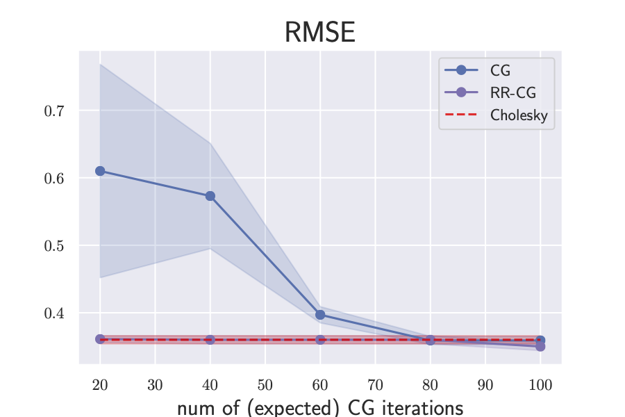
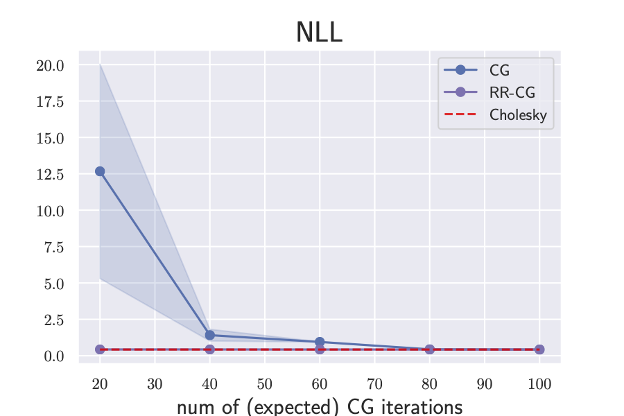
Figure S1: Predictive RMSE (left) and NLL (right) as a function of the number of (expected) CG iterations by optimizing Exact GP with CG (blue solid line) and RR-CG (purple solid line). Lower is better. The red dashed line corresponds to optimizing GP with Cholesky. The results are over three random seeds.

We provide the experiment details for the predictive performance experiments in Sec. 5.

Experiment setup.

To optimize the hyperparameters of the CG, RR-CG and Cholesky models, we use an Adam optimizer with learning rate = 0.01 and a MultiStepLR scheduler dropping the learning rate by a factor of 10 at the 50%, 70% and 90% of the optimization iterations. We run the optimization for 1500, 800 and 300 iterations on small (PoleTele, Elevators and Bike), medium (Kin40K, Protein, KEGG and KEGGU) and large (3DRoad) datasets, respectively. The number of iterations for CG and the expected number of iterations for RR-CG are both set to 100. The latter is achieved by using the truncation distribution from Eq. 17 with $\lambda=0.05$ and $J_{\min}=80$.

For CG and RR-CG, we use the rank-5 pivoted Cholesky preconditioner of Gardner et al. (2018). To reduce the number of optimization steps needed for the 3DRoad dataset, we initialize the hyperparameters to those found with the (biased) sgGP method. During evaluation, we compute the predictive mean using $1{,}000$ iterations of CG. Predictive variances are estimated using the rank-100 Lanczos approximation of Pleiss et al. (2018).

For RFF we use 1,000 random Fourier features across all experiments. In terms of optimization, we use an Adam optimizer with learning rate = 0.005 for KEGG, 0.001 for KEGGU and 0.01 for the remaining datasets. We also use a MultiStep scheduler that activates at 85%, 90%, 95% of the optimization iterations with a decay rate of 0.5 and also take a total of 500 optimization iterations on all the datasets.

In all the SVGP models we use $1{,}024$ inducing points, with a full-rank multivariate Gaussian variational distribution. Hyperparameters and variational parameters are jointly optimized for 300 epochs using minibatches of size $1{,}024$. As with the other baselines, we use the an Adam optimizer with a learning rate of $0.01$, dropping the learning rate by a factor of $10$ after 50%, 70% and 90% of the optimization iterations.

For sgGP, we train using minibatches of $16$ data points. As suggested by Chen et al. (2020), the minibatches are constructed by sampling one training data point and selecting its $15$ nearest neighbors. To accelerate optimization, we accumulate the gradients of $1{,}024$ minibatches before performing an optimization step (these $1{,}024$ minibatch updates can be performed in parallel, enabling GPU acceleration). We optimize the models for $300$ epochs, using the same learning rate and scheduler as with SVGP. During evaluation, we use the same procedure as for CC/RR-CG ($1{,}000$ iterations of CG, rank-$100$ Lanczos variance estimates).

For POE, we divide the training dataset into disjoint subsets, each with $M=1024$ data points. If $N$ is not divisible by $1024$, we pad the final subset with elements from the first subset. We train independent GP with independent hyperparameters on each of the subsets using the same optimization procedure as Cholesky models. Following Deisenroth & Ng (2015, Eqs. 11 and 12), the posterior distribution for a test input $\mathbf{x}^{*}$ is Gaussian with mean $\mu_{\text{POE}}^{*}(\mathbf{x}^{*})$ and variance $\sigma^{2*}_{\text{POE}}(\mathbf{x}^{*})$:

$$\mu^{*}_{\text{POE}}(\mathbf{x}^{*}) =\frac{\sigma^{2*}_{\text{POE}}(\mathbf{x}^{*})}{K}\sum_{k=1}^{K}\sigma^{-2*}_{k}(\mathbf{x}^{*})\mu^{*}_{k}(\mathbf{x}^{*}),$$

$$\sigma^{-2*}_{\text{POE}}(\mathbf{x}^{*}) =\frac{1}{K}\sum_{k=1}^{K}\sigma^{-2*}_{k}(\mathbf{x}^{*}),$$

where $K$ is the number of independent GP experts and $\mu^{*}_{k}(\cdot)$ and $\sigma^{2*}_{k}(\cdot)$ are the posterior mean and variance of each expert model.

Full tables.

In Table S1, we report the RMSE and NLL numbers which are used to plot Fig. 6 in the paper, and in Table S2 we report the corresponding training time.

Appendix F Additional Experiments

F.1 Predictive Performance with Different CG iterations

Here we include an additional experiment to show that early truncated CG can be detrimental to GP learning while RR-CG remains robust to the expected truncation number.

We conduct GP learning with the CG, RR-CG and Cholesky methods in the Elevators dataset. We vary the number of (expected) iterations for CG and RR-CG from 20 to 100 and plot the corresponding RMSE / NLL in Fig. S1. From the figure, we conclude that: 1) early truncation of the CG algorithm impedes GP optimization and leads to poor predictions. This problem lessens as we increase the number of CG iterations from 20 to 100. 2) The RR-CG model is robust to the expected truncation number, as it keeps comparable RMSE and NLL values to the Cholesky model under different expected truncation numbers. This experiment can only be run in smaller datasets to be able to compare against Cholesky. We chose Elevators as this dataset requires the largest number of CG iterations before convergence hence making the difference of choosing between CG and RR-CG evident. We emphasize that RR-CG is a better alternative to early-truncated CG as the latter can perform poorly in some cases, whereas the former is robust to the choice of expected truncation number.

F.2 Convergence of GP hypeparameters for other datasets.

In this section, we show how SS-RFF and RR-CG converge to the Cholesky solution whereas the biased methods do not. We make this analysis for other datasets than the ones used in the main manuscript.

Using RFF with $1{,}000$ or $1{,}500$ features generates results that clearly diverge from the Cholesky solution and RFF with a $1{,}000$ features generates numerically unstable training. In contrast, SS-RFF with $1{,}500$ features is able to achieve the Cholesky solution after $1{,}000$ iterations. Nonetheless, SS-RFF with $1{,}000$ features also suffers from numerical instability as RFF $1{,}000$ but at a lesser degree.

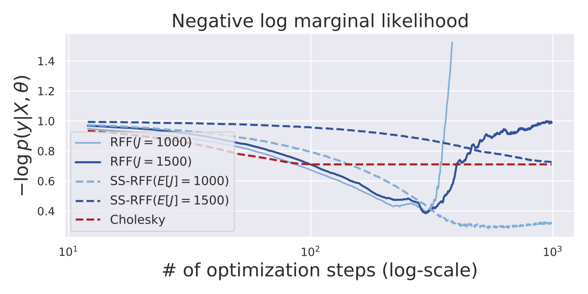
Figure S2: The GP optimization objective for models trained with RFF and SS-RFF. (Bike dataset, RBF kernel, Adam optimizer.) RFF models converge to sub-optimal log marginal likelihoods. SS-RFF models converge to (near) optimum values, yet require more than $100\times$ as many optimization steps.

The RR-CG models converge to optimal solutions, while the (biased) CG models diverge. Only the results for a low number of iterations is plotted since for more then 40 iterations CG and RR-CG are indistinguishable from Cholesky.

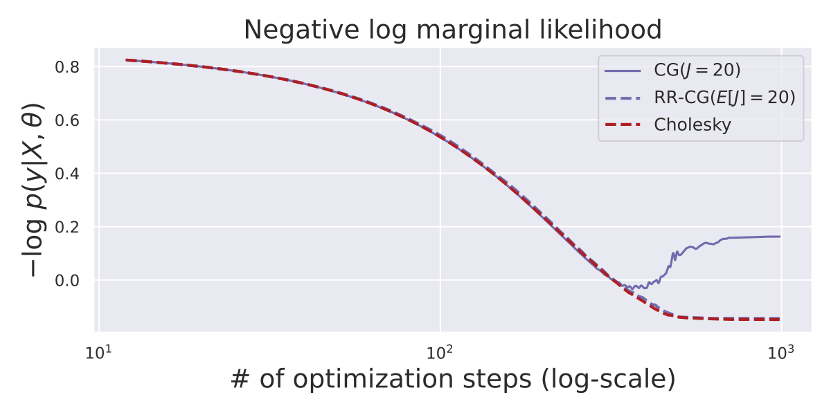
Figure S3: The GP optimization objective for models trained with CG and RR-CG. (PoleTele dataset, RBF kernel, Adam optimizer.) Models converge in $<100$ steps of Adam.

References

- Angelova (2012) Angelova, J. A. On moments of samples mean and variance. In Int. J. Pure Appl. Math, pp. 79:67–85, 2012.
- Asuncion & Newman (2007) Asuncion, A. and Newman, D. Uci machine learning repository, 2007.
- Bauer et al. (2016) Bauer, M., van der Wilk, M., and Rasmussen, C. E. Understanding probabilistic sparse gaussian process approximations. In Advances in Neural Information Processing Systems, 2016.
- Beatson & Adams (2019) Beatson, A. and Adams, R. P. Efficient optimization of loops and limits with randomized telescoping sums. In International Conference on Machine Learning, 2019.
- Bochner et al. (1959) Bochner, S. et al. Lectures on Fourier integrals, volume 42. Princeton University Press, 1959.
- Burt et al. (2019) Burt, D., Rasmussen, C. E., and Van Der Wilk, M. Rates of convergence for sparse variational gaussian process regression. In International Conference on Machine Learning, pp. 862–871, 2019.
- Cao & Fleet (2014) Cao, Y. and Fleet, D. J. Generalized product of experts for automatic and principled fusion of gaussian process predictions. arXiv preprint arXiv:1410.7827, 2014.
- Chen et al. (2020) Chen, H., Zheng, L., Al Kontar, R., and Raskutti, G. Stochastic gradient descent in correlated settings: A study on gaussian processes. Advances in Neural Information Processing Systems, 33, 2020.
- Chen et al. (2019) Chen, R. T. Q., Behrmann, J., Duvenaud, D., and Jacobsen, J.-H. Residual flows for invertible generative modeling. Advances in Neural Information Processing Systems, 2019.
- Cunningham et al. (2008) Cunningham, J. P., Shenoy, K. V., and Sahani, M. Fast gaussian process methods for point process intensity estimation. In International Conference on Machine learning, pp. 192–199, 2008.
- Cutajar et al. (2016) Cutajar, K., Osborne, M. A., Cunningham, J. P., and Filippone, M. Preconditioning kernel matrices. In International Conference on Machine Learning, 2016.
- Datta et al. (2016) Datta, A., Banerjee, S., Finley, A. O., and Gelfand, A. E. Hierarchical nearest-neighbor gaussian process models for large geostatistical datasets. Journal of the American Statistical Association, 111(514):800–812, 2016.
- Deisenroth & Ng (2015) Deisenroth, M. and Ng, J. W. Distributed gaussian processes. In International Conference on Machine Learning, pp. 1481–1490. PMLR, 2015.
- Dong et al. (2017) Dong, K., Eriksson, D., Nickisch, H., Bindel, D., and Wilson, A. G. Scalable log determinants for gaussian process kernel learning. In Advances in Neural Information Processing Systems, pp. 6327–6337, 2017.
- Filippone & Engler (2015) Filippone, M. and Engler, R. Enabling scalable stochastic gradient-based inference for gaussian processes by employing the unbiased linear system solver (ulisse). In International Conference on Machine Learning, pp. 1015–1024. PMLR, 2015.
- Gardner et al. (2018) Gardner, J., Pleiss, G., Weinberger, K. Q., Bindel, D., and Wilson, A. G. Gpytorch: Blackbox matrix-matrix gaussian process inference with gpu acceleration. In Advances in Neural Information Processing Systems, pp. 7576–7586, 2018.
- Golub & Meurant (2009) Golub, G. H. and Meurant, G. Matrices, moments and quadrature with applications, volume 30. Princeton University Press, 2009.
- Golub & Van Loan (2012) Golub, G. H. and Van Loan, C. F. Matrix Computations. The Johns Hopkins University Press, 4th Edition, 2012.
- Hensman et al. (2013) Hensman, J., Fusi, N., and Lawrence, N. D. Gaussian processes for big data. In Uncertainty in Artificial Intelligence, 2013.
- Hestenes et al. (1952) Hestenes, M. R., Stiefel, E., et al. Methods of conjugate gradients for solving linear systems. Journal of Research of the National Bureau of Standards, 49(1), 1952.
- Hutchinson (1989) Hutchinson, M. F. A stochastic estimator of the trace of the influence matrix for laplacian smoothing splines. Communications in Statistics-Simulation and Computation, 18(3):1059–1076, 1989.
- Kahn (1955) Kahn, H. Use of different monte carlo sampling techniques. Rand Corporation, 1955.
- Katzfuss et al. (2021) Katzfuss, M., Guinness, J., et al. A general framework for vecchia approximations of gaussian processes. Statistical Science, 36(1):124–141, 2021.
- Lanczos (1950) Lanczos, C. An iteration method for the solution of the eigenvalue problem of linear differential and integral operators1. Journal of Research of the National Bureau of Standards, 45(4), 1950.
- Loper et al. (2020) Loper, J., Blei, D., Cunningham, J. P., and Paninski, L. General linear-time inference for gaussian processes on one dimension. arXiv preprint arXiv:2003.05554, 2020.
- Luo et al. (2020) Luo, Y., Beatson, A., Norouzi, M., Zhu, J., Duvenaud, D., Adams, R. P., and Chen, R. T. Q. Sumo: Unbiased estimation of log marginal probability for latent variable models. In International Conference on Learned Representations, 2020.
- Lyne et al. (2015) Lyne, A.-M., Girolami, M., Atchadé, Y., Strathmann, H., Simpson, D., et al. On russian roulette estimates for bayesian inference with doubly-intractable likelihoods. Statistical science, 30(4):443–467, 2015.
- Mutnỳ & Krause (2018) Mutnỳ, M. and Krause, A. Efficient high dimensional bayesian optimization with additivity and quadrature fourier features. Advances in Neural Information Processing Systems, pp. 9005–9016, 2018.
- Nowozin (2018) Nowozin, S. Debiasing evidence approximations: On importance-weighted autoencoders and jackknife variational inference. In International Conference on Learned Representations, 2018.
- Oktay et al. (2020) Oktay, D., McGreivy, N., Aduol, J., Beatson, A., and Adams, R. P. Randomized automatic differentiation. arXiv preprint arXiv:2007.10412, 2020.
- Pleiss et al. (2018) Pleiss, G., Gardner, J. R., Weinberger, K. Q., and Wilson, A. G. Constant-time predictive distributions for gaussian processes. In International Conference on Machine learning, 2018.
- Rahimi & Recht (2008) Rahimi, A. and Recht, B. Random features for large-scale kernel machines. In Advances in Neural Information Processing Systems, pp. 1177–1184, 2008.
- Snelson & Ghahramani (2006) Snelson, E. and Ghahramani, Z. Sparse Gaussian processes using pseudo-inputs. In Advances in Neural Information Processing Systems, 2006.
- Sutherland & Schneider (2015) Sutherland, D. J. and Schneider, J. G. On the error of random fourier feaures. Conference on Uncertainty in Artificial Intelligence, 2015.
- Titsias (2009) Titsias, M. K. Variational learning of inducing variables in sparse Gaussian processes. In International Conference on Artificial Intelligence and Statistics, pp. 567–574, 2009.
- Ubaru et al. (2017) Ubaru, S., Chen, J., and Saad, Y. Fast estimation of tr(f(a)) via stochastic lanczos quadrature. SIAM Journal on Matrix Analysis and Applications, 38(4):1075–1099, 2017.
- Wang et al. (2019) Wang, K., Pleiss, G., Gardner, J., Tyree, S., Weinberger, K. Q., and Wilson, A. G. Exact gaussian processes on a million data points. In Advances in Neural Information Processing Systems, pp. 14648–14659, 2019.
- Wilson et al. (2020) Wilson, J., Borovitskiy, V., Terenin, A., Mostowsky, P., and Deisenroth, M. Efficiently sampling functions from gaussian process posteriors. In International Conference on Machine Learning, pp. 10292–10302, 2020.